Review

Phase Diagram and Critical Properties within an Effective Model of QCD: The Nambu–Jona-Lasinio Model Coupled to the Polyakov Loop

1
Centro de Física Computacional, Departamento de Física , Universidade de Coimbra, P-3004-516 Coimbra, Portugal
2
E.S.T.G., Instituto Politécnico de Leiria, Morro do Lena-Alto do Vieiro, 2411-901 Leiria, Portugal
3
IPNL, Université de Lyon/Université Lyon 1, CNRS/IN2P3, 4 rue E.Fermi, F-69622 Villeurbanne Cedex, France
*
Author to whom correspondence should be addressed.
Symmetry 2010, 2(3), 1338-1374; https://doi.org/10.3390/sym2031338
Submission received: 19 March 2010 / Revised: 27 May 2010 / Accepted: 2 July 2010 / Published: 6 July 2010
(This article belongs to the Special Issue Symmetry Breaking Phenomena)

Abstract

:
We investigate the phase diagram of the so-called Polyakov–Nambu–Jona-Lasinio model at finite temperature and non-zero chemical potential with three quark flavors. Chiral and deconfinement phase transitions are discussed and the relevant order-like parameters are analyzed. The results are compared with simple thermodynamic expectations and lattice data. We present the phase diagram in the ( T , μ B ) plane, paying special attention to the critical end point: as the strength of the flavor-mixing interaction becomes weaker, the critical end point moves to low temperatures and can even disappear.
Classification: PACS:
11.10.Wx; 11.30.Rd; 12.40.-y

1. Introduction

Symmetries play a fundamental role in physics. In fact, the modern fundamental physics is dominated by considerations underlying symmetries which can be exact, approximate (explicitly broken) and (spontaneously) broken. A special role is played by gauge or local symmetries which lead to the description of the “real world” as the so-called local/gauge theories with spontaneously broken symmetries.
The concept of spontaneous symmetry breaking has been transferred from condensed matter physics to quantum field theory by Nambu [1]. It has been introduced in particle physics on the grounds of an analogy with the breaking of (electromagnetic) gauge symmetry in the theory of superconductivity by Bardeen, Cooper and Schrieffer (the so-called BCS theory). The application of spontaneous symmetry breaking to particle physics in the 1960s and successive years led to profound physical consequences and played a fundamental role in the edification of several models of elementary particles.
Spontaneous breaking of chiral symmetry, in particular, is known to govern the low-energy properties of hadrons [2,3,4]. Some QCD-like models have been proposed before the advent of QCD, and the phenomenon of spontaneous breaking of chiral symmetry and Nambu–Goldstone theorem was established more than 40 years ago [1].
The Nambu–Jona-Lasinio (NJL) model was proposed in 1961 to explain the origin of the nucleon mass with the help of spontaneous breaking of chiral symmetry [5,6]. At that time, the model was formulated in terms of nucleons, pions and scalar sigma mesons. The introduction of the quark degrees of freedom and the description of hadrons by Eguchi and Kikkawa [7,8] in the chiral limit, where the bare quark mass is m 0 = 0 , and a more realistic version with m 0 0 by Volkov and Ebert [9,10,11], initiate a very intensive activity by several research groups [12].
There is strong evidence that quantum chromodynamics (QCD) is the fundamental theory of strong interactions. Its basic constituents are quarks and gluons that are confined in hadronic matter. It is believed that at high temperatures or densities the hadronic matter should undergo a phase transition into a new state of matter, the quark-gluon plasma (QGP). A challenge of theoretical studies based on QCD is to predict the equation of state, the critical point and the nature of the phase transition.
As the evolution of QCD at finite density/temperature is very complicated, QCD-like models, as for instance NJL type models, have been developed providing guidance and information relevant to observable experimental signs of deconfinement and QGP features. In fact, there has been great progress in the understanding of the properties of matter under extreme conditions of density and/or temperature, where the restoration of symmetries (e.g., the chiral symmetry) and the phenomenon of deconfinement should occur. These extreme conditions might be achieved in ultrarelativistic heavy-ion collisions or in the interior of neutron stars. In this context, increasing attention has been devoted to the study of the modification of particles propagating in a hot or dense medium [13,14]. The possible survival of bound states in the deconfined phase of QCD [15,16,17,18,19,20,21,22] has also opened interesting scenarios for the identification of the relevant degrees of freedom in the vicinity of the phase transition [23,24,25]. Besides lattice calculations [26,27,28,29], high temperature properties of QCD can be studied, starting from the QCD Lagrangian, within different theoretical schemes, like the dimensional reduction [30,31] or the hard thermal loop approximation [32,33,34]. Actually both the above approaches rely on a separation of momentum scales which, strictly speaking, holds only in the weak coupling regime g 1 . Hence they cannot tell us anything about what happens in the vicinity of the phase transition. On the other hand, a system close to a phase transition is characterized by large correlation lengths (infinite in the case of a second order phase transition). Its behavior is mainly driven by the symmetries of the Lagrangian, rather than by the details of the microscopic interactions.
Confinement and chiral symmetry breaking are two of the most important features of QCD. As already referred, chiral models like the NJL model [5,6,35,36] have been successful in explaining the dynamics of spontaneous breaking of chiral symmetry and its restoration at high temperatures and densities/chemical potentials. Recently, this and other type of models, together with an intense experimental activity, are underway to construct the phase diagram of QCD.
The actual NJL type models describe interactions between constituent quarks, giving the correct chiral properties, and offers a simple and practical illustration of the basic mechanisms that drive the spontaneous breaking of chiral symmetry, a key feature of QCD in its low temperature and density phase. In order to take into account features of both chiral symmetry breaking and deconfinement, static degrees of freedom are introduced in this Lagrangian through an effective gluon potential in terms of the Polyakov loop [37,38,39,40,41,42,43,44]. The coupling of the quarks to the Polyakov loop leads to the reduction of the weight of the quark degrees of freedom at low temperature as a consequence of the restoration of the Z N c symmetry associated with the color confinement.
In first approximation, the behavior of a system ruled by QCD is governed by the symmetry properties of the Lagrangian, namely the (approximate) global symmetry S U L ( N f ) × S U R ( N f ) , which is spontaneously broken to SU V ( N f ) , and the (exact) SU c ( N c ) local color symmetry. Indeed, in NJL type models the mass of a constituent quark is directly related to the chiral condensate, which is the order parameter of the chiral phase transition and, hence, is non-vanishing at zero temperature and density. Here the system lives in the phase of spontaneously broken chiral symmetry: the strong interaction, by polarizing the vacuum and turning it into a condensate of quark-antiquark pairs, transforms an initially point-like quark with its small bare mass m 0 into a massive quasiparticle with a finite size. Despite their widespread use, NJL models suffer a major shortcoming: the reduction to global (rather than local) color symmetry prevents quark confinement.
On the other hand, in a non-abelian pure gauge theory, the Polyakov loop serves as an order parameter for the transition from the low temperature, Z N c symmetric, confined phase (the active degrees of freedom being color-singlet states, the glueballs), to the high temperature, deconfined phase (the active degrees of freedom being colored gluons), characterized by the spontaneous breaking of the Z N c (center of SU c ( N c ) ) symmetry. With the introduction of dynamical quarks, this symmetry breaking pattern is no longer exact: nevertheless it is still possible to distinguish a hadronic (confined) phase from a QGP (deconfined) one.
In the PNJL model, quarks are coupled simultaneously to the chiral condensate and to the Polyakov loop: the model includes features of both chiral and Z N c symmetry breaking. The model has proven to be successful in reproducing lattice data concerning QCD thermodynamics [43]. The coupling to the Polyakov loop, resulting in a suppression of the unwanted quark contributions to the thermodynamics below the critical temperature, plays a fundamental role for the analysis of the critical behavior.
One of the important features of the QCD phase diagram is the existence of a phase boundary in the ( T , μ B ) that separates the chirally broken hadronic phase from the chirally symmetric QGP phase. Arguments based on effective model calculations suggest that the QCD phase diagram can exhibit a tricritical point (TCP)/critical end point (CEP) where the line of first order matches that of second order/analytical crossover [45,46,47,48,49,50]. The discussion about the existence and location of such critical points of QCD is a very important topic nowadays [51].
This paper is organized as follows. In Section 2 we analyze the main features and symmetries of QCD. In Section 3 we present the model and formalism starting with the deduction of the self consistent equations. We also obtain the equations of state and the response functions. The regularization procedure used in the model calculations is also included. Section 4 is devoted to the study of the equation of state at finite temperature. In Section 5 we study the phase diagram and the location of the critical end point. In Section 6 we discuss the important role of the choice of the model parameters for the correct description of isentropic trajectories. In Section 7 we analyze the effects of strangeness and anomaly strength on the location of the critical end point. In Section 8 we proceed to study the size of the critical region around the critical end point and its consequences for the susceptibilities. Finally, concluding remarks are presented in Section 9.

2. Symmetries of QCD

2.1. Quantum Chromodynamics

The Lagrangian of QCD is written as [52,53]
L Q C D = q ¯ ( i γ μ D μ m ^ ) q 1 4 F μ ν a F a μ ν
where q is the quark field with six flavors ( u , d , s , c , b , t ), three colors ( N c = 3 ) and m ^ being the corresponding current quark mass matrix in flavor space ( m ^ = diag f ( m u , m d , ) ). The covariant derivative,
D μ = μ i g t a A μ a
incorporates the color gauge field A μ a ( a = 1 , 2 , . . . , 8 ) and
F μ ν a = μ A ν a ν A μ a + g f a b c A μ b A ν c
is the gluon field strength tensor; t a is the Gell-Mann color matrix in SU(3) ( [ t a , t b ] = i f a b c t c , tr ( t a t b ) = δ a b 2 ) and f a b c are the corresponding antisymmetric structure constants. Finally, g is the QCD coupling constant.
The QCD Lagrangian is by construction symmetric under SU(3) gauge transformations in color space and because of the non-Abelian character of the gauge group QCD has some main features: it is a renormalizable quantum field theory [54] with a single coupling constant for both, the quark–gluon interactions and the gluonic self–couplings involving vertices with three and four gluons; it has confinement, i.e., objects carrying color like quarks and gluons do not exist as physical degrees of freedom in the vacuum. In addition, QCD is a theory that has asymptotic freedom [55,56], i.e., for large momenta, Q, or wavelengths of the order of 10 1 fm (ultraviolet region) the couplings are weak and the quarks and gluons propagate almost freely. For low momenta, or wavelengths of about 1 fm (infrared region), it happens the opposite situation and the couplings are quite strong. The system is now highly non perturbative. According to this property, the attraction between two quarks grows indefinitely as they move away from each other. This implies that the interaction between quarks and gluons can not be treated perturbatively, making the perturbative treatment of QCD not applicable to describe hadrons with masses below ∼2 GeV.
The low energy regime is specially interesting once it is relevant to the study of hadronic properties as for example in low energy QCD and nuclear physics.
The non-perturbative structure of the vacuum is characterized by the existence of quark condensates, i.e., it is expected non-zero values for the scalar density q ¯ q , by the appearance of light pseudoscalar particles, who are identified with (quasi) Goldstone bosons [57,58], and also by the existence of gluon pairs [59].
On the other hand, if QCD has a mechanism that includes the confinement of quarks the mass parameters m i are not observable quantities. However, they can be estimated in terms of the masses of some hadronic observables through current algebra’s methods. These masses are denominated by current quark masses to distinguish them from the constituent quark masses, which are effective masses generated by the spontaneous breaking of chiral symmetry in phenomenological models of quarks.

2.2. Chiral Symmetry Breaking

Due to the relevant role that spontaneous breaking of chiral symmetry plays in hadronic physics at low energies, this symmetry is one of most important symmetries of QCD. Here we will concentrate in the N f = 3 case. In the chiral limit, i.e. m u = m d = m s = 0 , QCD is chiral invariant which means that the QCD Lagrangian (1) is invariant under the group of symmetries:
U ( 3 ) L U ( 3 ) R = SU V ( 3 ) SU A ( 3 ) U V ( 1 ) U A ( 1 ) .
These symmetries are presented in Table 1 where it is also possible to see the transformations under which the Lagrangian is invariant, the currents that are conserved according to Noether’s theorem and the respective manifestations of the symmetries in nature.
The SU V (3) and U V (1) symmetries ensure the conservation of isospin and baryon number, respectively, while the SU A (3) and U A (1) symmetries are transformations that involve the γ 5 matrix and therefore alter the parity of the state in which they operate. For the sake of uniformity throughout the text we will designate by chiral symmetry the SU A (3) symmetry and by axial symmetry the U A (1) symmetry.
From the experimental point of view the manifestation of chiral symmetry would be the existence of parity doublets, i.e., a multiplet of particles with the same mass and opposite parity for each multiplet of isospin (the chiral partners), in the hadronic spectrum; that situation is not verified. Similarly, if the symmetry U A (1) would manifest itself, the existence of a partner with opposite parity to each hadron should be observed experimentally. As neither of these situations is observed in the hadron spectrum, these symmetries must be somehow broken.
Concerning the SU A (3) symmetry, the theory must contain a mechanism for the spontaneous breaking of chiral symmetry, which represents a transition to an asymmetric phase. This is closely related to the existence of non-zero quark condensates, q ¯ q , which are not invariant under SU A (3) transformations and therefore act as order parameters for the spontaneously broken chiral symmetry.
According to the Goldstone theorem, the spontaneous breaking of a continuous global symmetry implies the existence of a particle with zero mass, the Goldstone boson. In the case we are considering, the symmetry breaking is closely related to the appearance of eight degenerate Goldstone bosons with zero mass. As matter of fact the pions where the first mesons associated to Goldstone bosons due to their small mass. Indeed, if compared to the mass of the nucleon one has M π / M N = 0 . 15 . To reproduce the meson spectrum it is also necessary that the theory incorporates a mechanism which explicitly breaks the chiral symmetry: the Lagrangian must include perturbative terms that break ab initio the symmetry allowing the lifting of the degeneracy in the pseudoscalar mesons spectrum. These terms are the current quark masses m u m d and m s .
Nevertheless, the fundamentals of this process are not yet completely understood at the level of QCD. However, the chiral symmetry breaking, the generation of the constituent quark masses and the concomitant appearance of Goldstone bosons are explained in a very satisfactory way in certain theories and physical models like NJL type models.
Another symmetry effect occurs in the η η sector. The pseudoscalar η meson is not of the Goldstone type. Classically, the QCD Lagrangian with N f = 3 massless flavors possesses the U L ( 3 ) × U R ( 3 ) symmetry. In fact, the Adler–Jackiw–Bell U A ( 1 ) anomaly breaks this symmetry to SU L ( 3 ) × SU R ( 3 ) and yields a large mass for the η even if quark masses are zero. The origin of this anomaly are the instantons in QCD as explained in the next subsection.
In conclusion, QCD with three massless quarks possesses the SU L (3)× SU R (3) global chiral symmetry. At low energy, the pertinent degrees of freedom are mesons indicating that QCD experiences a confined/deconfined phase transition when energy increases. The study of mesons give us insight on the non-perturbative vacuum of QCD at low energy.

2.3. U A (1) Symmetry Breaking

Now we will analyze the U A (1) symmetry. It is known that in the chiral limit, and at the classical level, L Q C D is also invariant under the axial transformation (see Table 1).
As already mentioned, the absence in nature of chiral partners with the same mass, related with the U A (1) symmetry, opens the possibility that U A (1) symmetry is also spontaneously broken, similarly to what happens with the SU A (3) symmetry. Consequently, there should exist another pseudoscalar Goldstone boson. S. Weinberg estimated the mass of this particle, outside the chiral limit, at about 3 M π [60].
From all hadrons known in nature, the only candidates with the correct quantum numbers were the η ( 549 ) and η ( 985 ) . However, both violate the Weinberg estimate because their masses are too high: the η ( 985 ) has a mass comparable to the mass of nucleons (“ η problem”) and, furthermore, the η ( 549 ) is identified as belonging to the octet of pseudoscalar mesons. If a particle with the characteristics pointed out by Weinberg does not exist, then where is the ninth Goldstone boson? If this Goldstone boson does not exist there is no spontaneous breaking of U A (1) symmetry.
In 1976 G. ’t Hooft suggested that the U A (1) symmetry does not exist at the quantum level, being explicitly broken by the axial anomaly [60] which can be described at the semiclassical level by instantons [61,62]. Instantons are 4 D topologically stable soliton solutions of QCD. Other well known solitons are 2 D Abrikosov vortices in superconducting material or 3 D magnetic monopole in QCD. The instantons “transform” left handed fermions into right handed ones (and conversely). The transition induced by this solution of QCD has a non zero axial charge variation: Δ Q 5 = ± 2 N f , i.e., one left handed fermion ( + 1 in axial charge) transforms in a right handed fermion ( 1 ). To mimic this interaction in a purely fermionic effective theory, ’t Hooft proposed the following interaction Lagrangian, the so-called “’t Hooft determinant”:
L i n s t = κ e ı θ i n s t det f l a v o r ( ψ ¯ R ( x ) ψ L ( x ) ) + h . c .
This interaction “absorbs” N f left helicity fermions and converts them to right handed ones (and conversely). In the following, we will take θ i n s t = 0 .
In this context, as suggested by ’t Hooft, the instantons can play a crucial role in breaking explicitly the U A (1) symmetry giving to the η a mass of about 1 GeV outside the chiral limit. This implies that the mass of η has a different origin than the other masses of the pseudoscalar mesons and can not be seen as the missing Goldstone boson due to spontaneous breaking of U A (1) symmetry. Consequently, the U A (1) anomaly is very important once it is responsible for the flavor mixing effect that removes the degeneracy among several mesons.
Finally, an interesting open question also related to the symmetry that we wish to address is whether both chiral SU ( N f ) × SU ( N f ) and axial U A (1) symmetries are restored in the high temperature/density phase and which observables could carry information about these restorations.

2.4. The Polyakov Loop and the Z 3 Symmetry Breaking: Pure Gauge Sector

In this Section, following the arguments given in [38,39], we discuss how the deconfinement phase transition in a pure SU ( N c ) gauge theory can be conveniently described through the introduction of an effective potential for the complex Polyakov loop field, which we define in the following.
Since we want to study the SU ( N c ) phase structure, first of all an appropriate order parameter has to be defined. For this purpose the Polyakov line
L x P exp i 0 β d τ A 4 x , τ
is introduced. In the above, A 4 = i A 0 is the temporal component of the Euclidean gauge field ( A , A 4 ) , in which the strong coupling constant g has been absorbed, P denotes path ordering and the usual notation β = 1 / T has been introduced with the Boltzmann constant set to one ( k B = 1 ).
The Polyakov line L x can be described as an operator of parallel transport of the gauge field A 4 x , τ into the direction τ . One way to understand why this quantity is indeed a parameter that can distinguish between confined or deconfined phase is to consider the two extremal behavior of L: a color field A 4 at the point ( x , τ ) will be transformed into the color field L × A 4 after being transported into the direction τ . If L 1 it means that nothing affects the propagation of the field: the medium is in its deconfined phase. At the contrary L 0 indicates that the color field cannot propagate in the medium: it is confined.
Another way to see this point is to consider the variation of free energy when an infinitely massive (hence static) quark (that acts as a test color charge) is added to the system. To this purpose let us introduce the Polyakov loop. When the theory is regularized on the lattice, it reads:
l ( x ) = 1 N c Tr L ( x )
and it is a color singlet under SU ( N c ) , but transforms non-trivially, like a field of charge one, under Z N c . Its thermal expectation value can then be chosen as an order parameter for the deconfinement phase transition [63,64,65]: in the usual physical interpretation [66,67], l ( x ) is related to the change of free energy occurring when a heavy color source in the fundamental representation is added to the system. One has:
l ( x ) = e β Δ F Q ( x )
In the Z N c symmetric phase, l ( x ) = 0 , implying that an infinite amount of free energy is required to add an isolated heavy quark to the system: in this phase color is confined.
In the case of the SU ( 3 ) gauge theory, the Polyakov line L ( x ) gets replaced by its gauge covariant average over a finite region of space, denoted as L ( x ) [38,39]. Note that L ( x ) in general is not a SU ( N c ) matrix. The Polyakov loop field,
Φ ( x ) l ( x ) = 1 N c Tr c L ( x )
is then introduced.
Following the Landau-Ginzburg approach, a Z 3 symmetric effective potential is defined for the (complex) Φ field, which is conveniently chosen to reproduce, at the mean field level, results obtained in lattice calculations [38,39,43]. In this approximation one simply sets the Polyakov loop field Φ ( x ) equal to its expectation value Φ = c o n s t . , which minimizes the potential.
Concerning the effective potential for the (complex) field Φ , different choices are available in the literature [68,69,70]; the one proposed in [69] (see Equation (10)) is known to give sensible results [69,71,72] and will be adopted in our parametrization of the PNJL model that will be presented in Section 3. In particular, this potential reproduces, at the mean field level, results obtained in lattice calculations as it will be shown. The potential reads:
U Φ , Φ ¯ ; T T 4 = a T 2 Φ ¯ Φ + b ( T ) ln [ 1 6 Φ ¯ Φ + 4 ( Φ ¯ 3 + Φ 3 ) 3 ( Φ ¯ Φ ) 2 ]
where
a T = a 0 + a 1 T 0 T + a 2 T 0 T 2 and b ( T ) = b 3 T 0 T 3
The effective potential exhibits the feature of a phase transition from color confinement ( T < T 0 , the minimum of the effective potential being at Φ = 0 ) to color deconfinement ( T > T 0 , the minima of the effective potential occurring at Φ 0 ).
The parameters of the effective potential U are given in Table 2. These parameters have been fixed in order to reproduce the lattice data for the expectation value of the Polyakov loop and QCD thermodynamics in the pure gauge sector [73,74].
The parameter T 0 is the critical temperature for the deconfinement phase transition within a pure gauge approach: it was fixed to 270 MeV, according to lattice findings. Different criteria for fixing T 0 may be found in the literature, like in [75], where an explicit N f dependence of T 0 is presented by using renormalization group arguments. However, it is noticed that the Polyakov loop computed on the lattice with (2+1) flavors and with fairly realistic quark masses is very similar to the SU f (2) case [74]. Hence, it was chosen to keep for the effective potential U Φ , Φ ¯ ; T the same parameters which were used in SU f (2) PNJL [69], including T 0 = 270 MeV. The latter choice ensures an almost exact coincidence between chiral crossover and deconfinement at zero chemical potential, as observed in lattice calculations. We notice, however, as it will be seen in Section 4, that a rescaling of T 0 to 210 MeV may be needed in some cases in order to get agreement between model calculations and thermodynamic quantities obtained on the lattice. Let us stress that this modification of T 0 (the only free parameter of the Polyakov loop once the effective potential is fixed) is essentially done for rescaling reasons (an absolute temperature scale has not a very strong meaning in these kind of Ginzburg–Landau model based on symmetry) but does not change drastically the physics.
With the present choice of parameters, Φ and Φ ¯ are always lower than 1 in the pure gauge sector. In any case, in the range of applicability of our model, T ( 2 3 ) T c , there is a good agreement between the results and the lattice data for Φ .
To conclude this section, some comments are in order on the number of parameters and the nature of the Polyakov field.
It should be noticed that the NJL parameters and the Polyakov potential ones are not on the same footing. Whereas the NJL parameters are directly related in a one to one correspondence with a physical quantity, the Polyakov loop potential is there to insure that the pure gauge lattice expectations are recovered. Hence the potential for the loop can be viewed as a unique but functional parameter. The details of this function are not very important to study the thermodynamic as soon as the potential reproduces the lattice results. In order to clarify this point, we remember that in a previous calculations in the N f = 2 case [76] we used two kind of potentials and obtained very small differences in what concerns thermodynamics; however, if one calculates susceptibilities with respect to Φ the log potential used here has to be preferred in order not to have unphysical results. The only true parameter is the pure gauge critical temperature T 0 that fixes the temperature scale of the system. However we would like to point out that it is expected in the Landau-Ginzburg framework that a characteristic temperature for a phase transition will not be a prediction: one needs to fix the correct energy scale somehow and it is the role of this parameter. Hence we will allow ourselves to change this parameter in the calculation of some observables in order to compare our results with lattice QCD expectations.
Finally we want to stress that, contrarily to the full Landau-Ginzburg effective field approach, the Polyakov loop effective field is not a dynamical degree of freedom due to the the lack of dynamical term in the Polyakov loop potential. Hence it is a background gauge field in which quarks will propagate. Anyway the potential mimics a pressure term that has the correct magnitude and temperature behavior in order to get the Stefan-Boltzman limit for the gluonic degrees of freedom and that explains the success of the model.

2.5. QCD Phase Diagram

Understanding the QCD phase structure is one of the most important topics in the physics of strong interactions. The developed effort on both the theoretical point of view—using effective models and lattice calculations—and the experimental point of view is one of the main goals of the heavy ion collisions program; it has proved very fruitful, shedding light on properties of matter at finite temperatures and densities.
From the theoretical point of view, the physics of the transition from hadronic matter to the QGP is well established for baryonic chemical potential μ B = 0 . Latest lattice results for (2+1) flavors show a crossover transition at T c = ( 170 200 ) MeV (using m q = 0 . 05 m s ) [77]. Near the critical temperature, T c , the energy density (and other thermodynamic quantities) show a strong growth, signaling the transition from a hadronic resonance gas to a matter of deconfined quarks and gluons. As matter of fact, the rapid rise of the energy density is usually interpreted to be due to deconfinement i.e., liberation of many new degrees of freedom. In the limit where quark masses are infinitely heavy the order parameter for the deconfinement phase transition is the Polyakov loop. A rapid change in this quantity is also an indication for deconfinement even in the presence of light quarks [77].
Concerning chiral symmetry, and considering the chiral limit, it is expected a chiral transition with the corresponding order parameter being the quark condensate: the quark condensate vanishes at the critical temperature T c and a genuine phase transition takes place. Even away from the chiral limit, when the quark masses are finite, it is expected, in the transition region, a “crossover” where the quark condensates rapidly drop indicating a partial restoration of the chiral symmetry [77].
This rises the interesting question whether the restoration of chiral symmetry and the transition to the QGP occurs at same time. In [78] it was proposed that the evidence of restoration of chiral symmetry is a sufficient condition to demonstrate the existence of a new state of matter, but it is not a necessary condition for the discovery of the QGP. In fact, as already pointed out, most of lattice results shows a tendency for the restoration of chiral symmetry to happen simultaneously with deconfinement, but this issue is not definitively determined from a theoretical point of view.
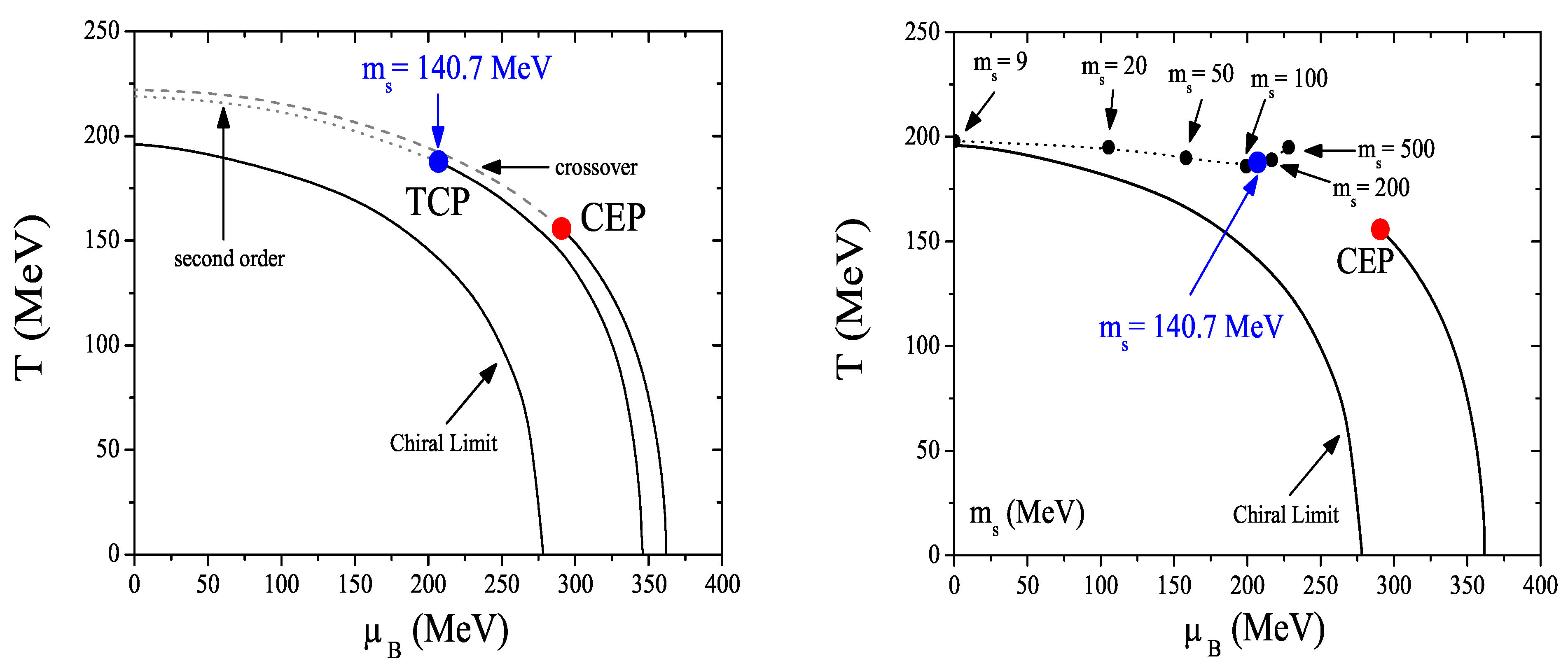
At finite temperature and chemical potential the most common three-flavor phase diagram shows a first order boundary of the chiral phase transition separating the hadronic and quark phases. This first–order line starts at non-zero chemical potential and zero temperature and will finish in a point, the critical end point ( T C E P , μ B C E P ), where the phase transition is of second order. As the temperature increases and the chemical potential decreases, the QCD phase transition becomes a crossover.
Although recent lattice QCD results by de Forcrand and Philipsen question the existence of the CEP [79,80,81], this critical point of QCD, proposed at the end of the eighties [45,46,47,48], is still a very important subject of discussion nowadays [51]. The search of the QCD CEP is one of the main goals in “Super Proton Synchrotron” (SPS) at CERN [82] and in the next phase of the “Relativistic Heavy Ion Collider” (RHIC) running at BNL.
When matter at high density and low temperature is considered, it is expected that this type of matter is a color superconductor where pairs of quarks condense (“diquark condensate”): this color superconductor is a degenerate Fermi gas of quarks with a condensate of Cooper pairs near the Fermi surface that induces color Meissner effects. With the color superconductivity it was realized that the consideration of diquark condensates opened the possibility for a wealth of new phases in the QCD phase diagram. At the highest densities/chemical potentials, where the QCD coupling is weak, the ground state is a particularly symmetric state, the color-flavor locked (CFL) phase: up, down, and strange quarks are paired in a so-called color-flavor locked condensate. At lower densities the CFL phase may be disfavored in comparison with alternative new phases which may break translation and/or rotation invariance [36,83].
Recently it was argued that some features of hadron production in relativistic nuclear collisions, mainly at SPS–CERN energies, can be explained by the existence of a new form of matter beyond the hadronic matter and the QGP: the so-called quarkyonic matter [70,84,85,86]. It was also suggested that these different types of matter meet at a triple point in the QCD phase diagram: both the hadronic matter, the QGP, and the quarkyonic matter all coexist [87].
From the experimental point of view, different parts of the QCD phase diagram have been investigated for different beam energies. For high energies, corresponding to the energies of RHIC–BNL and LHC–CERN (“Large Hadron Collider”), the matter is produced at high temperature and low baryonic density [78,88,89]. On the other hand, intermediate energy, corresponding to the energies of “Alternating Gradient Synchrotron” (AGS) in BNL or in SPS–CERN [82], can be studied through matter formed at moderate temperature and baryonic density. Finally, the energies achieved in the GSI Heavy Ion Synchrotron (SIS) [90] and “Nuclotron-based Ion Collider fAcility” (NICA) at JINR [
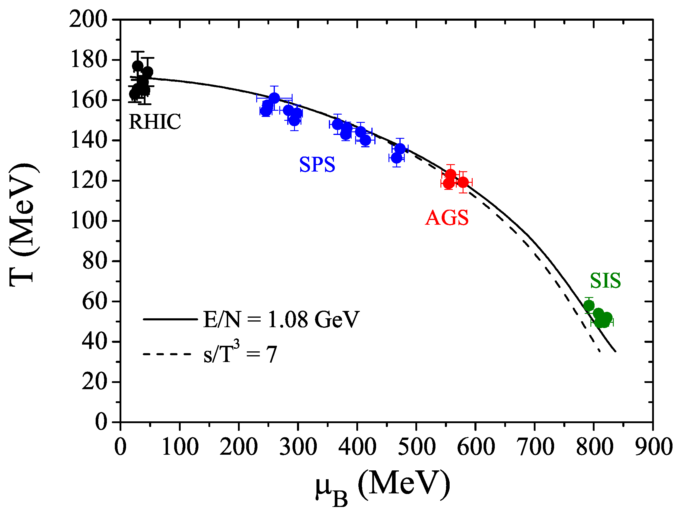
91] will allow to obtain matter at low temperatures and high baryonic densities. For example the main goal of the research program on nucleus-nucleus collisions at GSI is the investigation of highly compressed nuclear matter. Matter in this form exists in neutron stars and in the core of supernova explosions.
In Figure 1 are indicated the points where the hadrons cease to interact with each others (freeze-out points) for the different beam energies. These points are related to final state of the expansion of the fireball.
It should also be noted that atomic nuclei by themselves represent a system at finite density and zero temperature. At normal nuclear density it is estimated that the quark condensate undergoes a reduction of 30 % [93] so that the resulting effects in the chiral order parameter can be measured in beams of hadrons, electrons and photons in nuclear targets.
If the evidence for deconfinement can be found experimentally, then the search for manifestations of chiral symmetry restoration will be, in the near future, one of the main goals once the investigation of the properties of matter can provide a clear evidence for changes in the fundamental vacuum of QCD, with far-reaching consequences [78].

3. The PNJL Model with Three Flavors

The Polyakov–Nambu–Jona-Lasinio (PNJL model) that we want to build is an effective model for QCD, written in term of quark degrees of freedom. In the next paragraphs we will present the ingredients we need to build our model namely: a massive Dirac Lagrangian together with a four quark chirally invariant interaction (the original NJL Lagrangian with a small mass term that breaks explicitly the chiral symmetry, has observed in the mass spectrum); the so-called ’t Hooft interaction that reproduces the interaction of quarks with instantons and finally a Polyakov loop potential that mimic the effect of the pure gauge (Yang-Mills) sector of QCD on the quarks.

3.1. Nambu–Jona-Lasinio Model with Anomaly and Explicit Symmetry Breaking

Phase transitions are usually characterized by large correlation lengths, i.e., much larger than the average distance between the elementary degrees of freedom of the system. Effective field theories then turn out to be a useful tool to describe a system near a phase transition. In particular, in the usual Landau-Ginzburg approach, the order parameter is viewed as a field variable and for the latter an effective potential is built, respecting the symmetries of the original Lagrangian. The existence of a phase transition between two sectors where the chiral symmetry is spontaneously broken or restored (transition associated to the quark condensate that acts as an order parameter) and the Ginzburg–Landau theory suggests to use the symmetry motivated NJL Lagrangian [35,36,59,94] for the description of the coupling between quarks and the chiral condensate in the scalar-pseudoscalar sector. The associated Lagrangian which complies with the underlying symmetries of QCD described in the previous section reads:
L N J L = L 0 + L 4 + L 6
L 0 = q ¯ ( i γ μ μ m ^ ) q
L 4 = 1 2 g S a = 0 8 [ ( q ¯ λ a q ) 2 + ( q ¯ i γ 5 λ a q ) 2 ]
L 6 = g D { det [ q ¯ ( 1 + γ 5 ) q ] + det [ q ¯ ( 1 γ 5 ) q ] }
In the above q = ( u , d , s ) is the quark field with three flavors ( N f = 3 ) and three colors ( N c = 3 ), m ^ = diag ( m u , m d , m s ) is the current quark mass matrix, and λ a are the flavor SU f (3) Gell-Mann matrices ( a = 0 , 1 , , 8 ), with λ 0 = 2 3 I .
As it is well known, this Lagrangian is invariant under a global—and nonlocal—color symmetry S U ( N c = 3 ) and lacks the confinement feature of QCD.
L 4 has U L ( 3 ) × U R ( 3 ) chiral symmetry and L 6 is a six quarks interaction, the ’t Hooft determinant to reproduce U A ( 1 ) anomaly. The U L ( 3 ) × U R ( 3 ) symmetry of L 0 + L 4 is broken to S U L ( 3 ) × S U R ( 3 ) by L 6 .
The current quark mass matrix m ^ is in general non degenerate and explicitly breaks chiral symmetry S U L ( 3 ) × S U R ( 3 ) to S U f ( 3 ) or its subgroup. In the following we will take m u = m d hence keeping exact the isospin symmetry.
Let us notice that NJL has no build-in confinement and is non-renormalizable thus it requires the introduction of a cutoff parameter Λ .
The parameters, obtained by following the methodology of [95], are: m u = m d = 5 . 5 MeV, m s = 140 . 7 MeV, g S Λ 2 = 3 . 67 , g D Λ 5 = 12 . 36 and Λ = 602 . 3 MeV, which are fixed to reproduce the values of the coupling constant of the pion, f π = 92 . 4 MeV, and the meson masses of the pion, the kaon, the η and η , respectively, M π = 135 MeV, M K = 497 . 7 MeV, M η = 514 . 8 MeV and M η = 960 . 8 MeV.

3.2. Coupling between Quarks and the Gauge Sector: The PNJL Model

In the presence of dynamical quarks the Z 3 symmetry is explicitly broken: the expectation value of the Polyakov loop still serves as an indicator for the crossover between the phase where color confinement occurs ( Φ 0 ) and the one where color is deconfined ( Φ 1 ).
The PNJL model attempts to describe in a simple way the two characteristic phenomena of QCD, namely deconfinement and chiral symmetry breaking.
In order to describe the coupling of quarks to the chiral condensate, we start from a NJL description of quarks; they are coupled in a minimal way to the Polyakov loop, via a covariant derivative. Hence our calculations are performed in the framework of an extended SU f (3) PNJL Lagrangian, which includes the ’t Hooft instanton induced interaction term that breaks the U A (1) symmetry and the quarks are coupled to the (spatially constant) temporal background gauge field Φ [70,96,97]. The Lagrangian reads:
L P N J L = q ¯ ( i γ μ D μ m ^ ) q + 1 2 g S a = 0 8 [ ( q ¯ λ a q ) 2 + ( q ¯ i γ 5 λ a q ) 2 ] + g D { det [ q ¯ ( 1 + γ 5 ) q ] + det [ q ¯ ( 1 γ 5 ) q ] } U Φ [ A ] , Φ ¯ [ A ] ; T
The covariant derivative is defined as D μ = μ i A μ , with A μ = δ 0 μ A 0 (Polyakov gauge); in Euclidean notation A 0 = i A 4 . The strong coupling constant g is absorbed in the definition of A μ ( x ) = g A a μ ( x ) λ a 2 , where A a μ is the (SU c (3)) gauge field and λ a are the (color) Gell-Mann matrices.
At T = 0 , it can be shown that the minimization of the grand potential leads to Φ = Φ ¯ = 0 . So, the quark sector decouples from the gauge one, and the model is fixed as referred in the previous subsection.
Some remarks are in order concerning the applicability of the PNJL model. It should be noticed that in this model, beyond the chiral point-like coupling between quarks, the gluon dynamics is reduced to a simple static background field representing the Polyakov loop (see details in [44,68]). This scenario is expected to work only within a limited range of temperatures, since at large temperatures transverse gluons are expected to start to be thermodynamically active degrees of freedom and they are not taken into account in the PNJL model. We can assume that the range of applicability of the model is roughly limited to T ( 2 3 ) T c , since, as concluded in [98], transverse gluons start to contribute significantly for T > 2 . 5 T c , where T c is the deconfinement temperature.

3.3. Grand Potential in the Mean Field Approximation

Our model of strongly interacting matter can simulate either a region in the interior of neutron stars or a dense fireball created in a heavy-ion collision. In the present work, we focus our attention on the last type of systems. Bearing in mind that in a relativistic heavy-ion collision of duration of about 10 22 s , thermal equilibration is possible only for processes mediated by the strong interaction rather than the full electroweak equilibrium, we impose the condition μ e = 0 and use the chemical equilibrium condition μ u = μ d = μ s = μ . This choice allows for isospin symmetry, m u = m d and approximates the physical conditions at RHIC.
We will work in the (Hartree) mean field approximation. In this context, the quarks can be seen as free particles whose bare current masses m i are replaced by the constituent (or dressed) masses M i .
The quark propagator in the constant background field A 4 is then:
S i ( p ) = ( p M i + γ 0 ( μ i A 4 ) ) 1
In the above, p 0 = i ω n and ω n = ( 2 n + 1 ) π T is the Matsubara frequency for a fermion.
Within the mean field approximation, it is straightforward (see Ref. [35]) to obtain effective quark masses from the Lagrangian (16); these masses are given by the so-called gap equations:
M i = m i 2 g S q i ¯ q i 2 g D q j ¯ q j q k ¯ q k
where the quark condensates q i ¯ q i , with i , j , k = u , d , s (to be fixed in cyclic order), have to be determined in a self-consistent way as explained in the Appendix.
The PNJL grand canonical potential density in the SU f (3) sector can be written as
Ω = Ω ( Φ , Φ ¯ , M i ; T , μ ) = U Φ , Φ ¯ , T + g S i = u , d , s q i ¯ q i 2 + 4 g D q u ¯ q u q d ¯ q d q s ¯ q s 2 N c i = u , d , s Λ d 3 p 2 π 3 E i 2 T i = u , d , s d 3 p 2 π 3 z Φ + ( E i ) + z Φ ( E i )
where E i is the quasi-particle energy for the quark i: E i = p 2 + M i 2 , and z Φ + and z Φ are the partition function densities.
The explicit expression of z Φ + and z Φ are given by:
z Φ + ( E i ) Tr c ln 1 + L e β E p = ln 1 + 3 Φ ¯ + Φ e β E p e β E p + e 3 β E p
z Φ ( E i ) Tr c ln 1 + L e β E p + = ln 1 + 3 Φ + Φ ¯ e β E p + e β E p + + e 3 β E p +
where E i ( ± ) = E i μ , the upper sign applying for fermions and the lower sign for anti-fermions. The technical details are postponed to the Appendix but as a conclusion on this topic, a word is in order to describe the role of the Polyakov loop in the present model. Almost all physical consequences of the coupling of quarks to the background gauge field stem from the fact that in the expression of z Φ , Φ or Φ ¯ appear only as a factor of the one- or two-quarks (or antiquarks) Boltzmann factor, for example e β E p + and e 2 β E p + . Hence when Φ , Φ ¯ 0 (signaling what we designate as the “confined phase”) only e 3 β E p + remains in the expression of the grand potential, leading to a thermal bath with a small quark density. At the contrary Φ , Φ ¯ 1 (in the “deconfined phase”) gives a thermal bath with all 1-, 2- and 3-particle contributions and a significant quark density. Other consequences of this coupling of the loop to the 1- and 2-particles Boltzmann factor will be discussed in Section 8.

3.4. Equations of State and Response Functions

The equations of state can be derived from the thermodynamical potential Ω ( T , μ ) . This allows for the comparison of some of the results with observables that have become accessible in lattice QCD at non-zero chemical potential.
As usual, the pressure p is defined such as its value is zero in the vacuum state [36] and, since the system is uniform, we have
p ( T , μ ) = 1 V [ Ω ( T , μ ) Ω ( 0 , 0 ) ]
where V is the volume of the system.
The relevant observables are the baryonic density
ρ B ( T , μ ) = 1 V Ω μ T
and the (scaled) “pressure difference” given by
Δ p ( T , μ ) T 4 = p ( T , μ ) p ( T , 0 ) T 4
Due to the relevance for the study of the thermodynamics of matter created in relativistic heavy-ion collisions, it is interesting to perform an analysis of the isentropic trajectories. The equation of state for the entropy density, s, is given by
s ( T , μ ) = p T μ
and the energy density, ϵ , comes from the following fundamental relation of thermodynamics
ϵ ( T , μ ) = T s ( T , μ ) + μ ρ B ( T , μ ) p ( T , μ )
The energy density and the pressure are defined such that their values are zero in the vacuum state [36].
The baryon number susceptibility, χ B , and the specific heat, C, are the response of the baryon number density, ρ B ( T , μ ) , and the entropy density, s ( T , μ ) , to an infinitesimal variation of the quark chemical potential μ and temperature, given respectively by:
χ B = ρ B μ T and C = T V s T μ
These second order derivatives of the pressure are relevant quantities to discuss phase transitions, mainly the second order ones.

3.5. Model Parameters and Regularization Procedure

As already seen, the pure NJL sector involves five parameters: the coupling constants g S and g D , the current quark masses m u = m d , m s and the cutoff Λ defined in Section 3. These parameters are determined in the vacuum by fitting the experimental values of several physical quantities. We notice that the coupling constant g S and g D and the parameter Λ are correlated. For instance, if we increase g S in order to provide a more significant attraction between quarks, we must also increase the cutoff Λ in order to insure a good agreement with experimental results. In addition, the value of the cutoff itself does have some impact as far as the medium effects in the limit T = 0 are concerned. Also the strength of the coupling g D has a relevant role in the location of the CEP, as it will be discussed.
In fact, the choice of the parametrization may give rise to different physical scenarios at T = 0 and μ B = μ 0 [36], even if they give reasonable fits to hadronic vacuum observables and predict a first order phase transition. The set of parameters we used insures the stability conditions and, consequently, the compatibility with thermodynamic expectations.
On the other hand, the regularization procedure, as soon as the temperature effects are considered, has relevant consequences on the behavior of physical observables, namely on the chiral condensates and the meson masses [99]. Advantages and drawbacks of these regularization procedures have been discussed within the NJL [99] and PNJL [76,
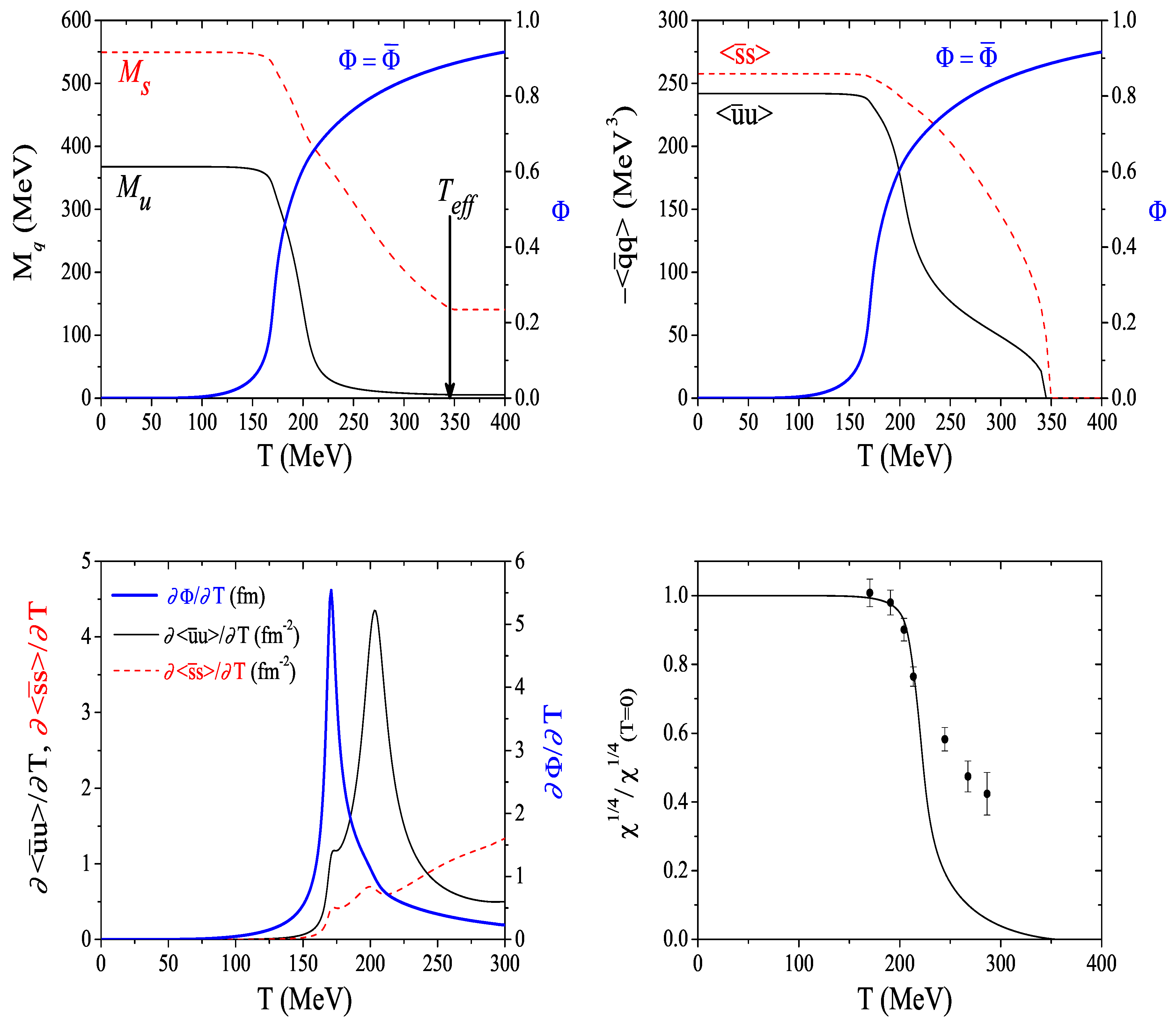
100] models. We remind that one of the drawbacks of the regularization that consists in putting a cutoff only on the divergent integrals is that, at high temperature, there is a too fast decrease of the quark masses that become lower than their current values. This leads to a non physical behavior of the quark condensates that, after vanishing at the temperature ( T e f f ) where constituent and current quark masses coincide, change sign and acquire non-zero values again. To avoid this unphysical effects we use the approximation of imposing by hand the condition that, above T e f f , M i = m i and q i ¯ q i = 0 .

4. Equation of State at Finite Temperature

4.1. Characteristic Temperatures

At zero temperature and chemical potential, the chiral symmetry of QCD is explicitly broken. It is expected that chiral symmetry will be restored at high temperature; hence a phase transition occurs separating the low and the high temperature regions. This phenomena may be realized in high energy heavy ion collision experiments.
In this case ( μ B = 0 and T 0 ), where a crossover transition occurs in the PNJL model, a unique critical temperature cannot be defined, but one of many characteristic temperatures for the transition may be used. Of course, these temperatures should coincide in the limit where the transition becomes of second order (in the chiral limit, for example, when one is concerned with the restoration of chiral symmetry).
We start our analysis by identifying the characteristic temperatures which separate the different thermodynamic phases in the PNJL model [44], using the regularization that allows high momentum quark states at finite temperature (the cutoff is used only in the integrals that are divergent and Λ in the ones that are already convergent because of the thermal distributions).
Let us analyze the behavior of the quark masses and the field Φ . The characteristic temperature related to the deconfinement phase transition is T c Φ and the chiral phase transition characteristic temperature, T c χ , signals partial restoration of chiral symmetry. These temperatures are chosen to be, respectively, the inflexion points of the “quasi” order parameter Φ and of the chiral condensate q u ¯ q u ; as in [68], we define T c as the average of the two transition temperatures, T c Φ and T c χ . As shown in [100], the present regularization lowers the characteristic temperatures and decreases the gap T c Φ T c χ , leading therefore to better agreement with lattice results.
Let us remark that this section is also devoted to the study of thermodynamic quantities (pressure, energy per particle and entropy) for which a rescaling of the temperature T 0 is needed, in order to get a better agreement with lattice results for these quantities. Therefore, following the argumentation presented in [68], here we will use the reduced temperature T c by rescaling the parameter T 0 from 270 to 210 MeV (let us stress that this rescaling is only done for the remainder of this section). Results for the characteristic temperatures with T 0 = 210 MeV and T 0 = 270 MeV are shown in Table 3.
It should be noticed that, when T 0 = 210 MeV is used, we loose the almost perfect coincidence of the chiral and deconfinement transitions (they are shifted relative to each other by about 32 MeV) and we have T c = 187 MeV within the range expected from lattice calculations [77]. However, the behavior of the relevant physical quantities is qualitatively the same whether T 0 = 270 MeV or T 0 = 210 MeV.
An interesting point to be noticed in Figure 2, lower panel, is that the inflexion points of the strange and non-strange quark condensates are close and slightly separated from the inflexion point of Φ , although the condensates have small peaks around the inflexion point of Φ . The latter effect is related to the fastening of the phase transition induced by the Polyakov loop as shown in [102] (it obviously does not signal a phase transition since the variation of the order parameter around this temperature is small). The Polyakov loop leads to a faster decrease of the quark masses around T c and the present regularization enhances this effect, even at temperatures higher than T c . At T e f f = 345 MeV the regularization is responsible for the full restoration of the chiral symmetry that was dynamically broken: the quark masses go to their current values and the quark condensates vanish (see Figure 2, left and right panels). As already shown in the framework of the pure NJL model [99] and in the PNJL model [100], the effect of allowing high momentum quark states is stronger for the strange quark mass. Indeed, with the conventional regularization, the non-strange constituent quark mass at high temperature is already very close to its current mass, the new regularization only enhancing this behavior. Differently, the strange quark mass is always far from its current value, unless we allow high momentum quarks to be present and, in that case, its constituent mass decreases very substantially and comes to its current value.
As shown in [100], at T e f f the behavior of some given observables signals the effective restoration of chiral and axial symmetry: the masses of the meson partners of both chiral and axial symmetry are degenerated and the topological susceptibility vanishes as we can see from Figure 2 (lower right panel).

4.2. Thermodynamic Quantities

In the limit of vanishing quark chemical potential, significant information on the phase structure of QCD at high temperature is obtained from lattice calculations. The transition to the phase characteristic of this regime is related with chiral and deconfinement transitions which are the main features of our model calculation.
In Figure 3, we plot the scaled pressure, the energy and the entropy as functions of the temperature compared with recent lattice results (see Reference [77]). Since the transition to the high temperature phase is a rapid crossover rather than a phase transition, the pressure, the entropy and the energy densities are continuous functions of the temperature. We observe a similar behavior in the three curves: a sharp increase in the vicinity of the transition temperature and then a tendency to saturate at the corresponding ideal gas limit. Asymptotically, the QCD pressure for N f massless quarks and ( N c 2 1 ) massless gluons is given ( μ B = 0 ) by:
p S B T 4 = ( N c 2 1 ) π 2 45 + N c N f 7 π 2 180 ,
where the first term denotes the gluonic contribution and the second term the fermionic one.
The results follow the expected tendency and go to the free gas values (or Stefan–Boltzmann limit), a feature that was also found with this type of regularization in the context of the SU(2) PNJL model [68,103,104]. The inclusion of the Polyakov loop effective potential U ( Φ , Φ ¯ ; T ) (it can be seen as an effective pressure term mimicking the gluonic degrees of freedom of QCD) is required to get the correct limit (indeed in the NJL model the ideal gas limit is far to be reached due to the lack of gluonic degrees of freedom).
The inclusion of the Polyakov loop and the regularization procedure are essential to obtain the required increase of extensive thermodynamic quantities, insuring the convergence to the Stefan-Boltzmann (SB) limit of QCD [105]. Some comments are in order concerning the role of the regularization procedure for T > T c . In this temperature range, due to the presence of high momentum quark states, the physical situation is dominated by the significant decrease of the constituent quark masses by the q q ¯ interactions. This allows for an ideal gas behavior of almost massless quarks with the correct number of degrees of freedom.
Let us notice that, just below T c , the pressure and the energy fail to reproduce the lattice points: for example there is a small underestimation of the pressure and energy in the model calculations. It is known that the lack of mesonic correlations in the PNJL model is responsible for, at least, a fraction of this discrepancy. As matter of fact, in [106] the authors have evaluated the pion and sigma contributions to the pressure by calculating the ring sum in the SU(2) nonlocal PNJL model. They have shown that the pionic contribution dominates the pressure in the low temperature region, shifting the respective curve to higher values. It is expected that the introduction of mesonic correlations in the SU(3) PNJL model has the same effect for the pressure.

5. Phase Diagram and the Location of the Critical End Point

Although recent lattice QCD results by de Forcrand and Philipsen question the existence of the CEP [79,80,81], this critical point of QCD, proposed at the end of the eighties [45,46,47,48], is still a very important subject of discussion nowadays [51].
We remember that the TCP separates the second order transition at high temperature and low chemical potential, from the first order transition at high chemical potential and low temperature. If the second order transition is replaced by a smooth crossover, a CEP which separates the two lines is found. In order to determine and elucidate the nature of the phase transition the relevant thermodynamic quantities are studied, starting with zero temperature and finite chemical potential.

5.1. Phase Transition at Zero Temperature

Figure 4 illustrates the properties of cold quark matter as predicted by the model calculation. In the left panel the negative of the thermodynamic potential is plotted as a function of the chemical potential, showing the presence of branches with stable, metastable and unstable solutions. This behavior is obtained in the domain μ B 2 < μ B < μ B 1 , where the gap equations (18) have three solutions as illustrated in the left panel of Figure 4 for the constituent non-strange quark mass. As a consequence, a first order phase transition is found at the critical chemical potential μ B c r = 361 . 7 MeV. The stable solutions are realized by the minimum of the thermodynamic potential. When stable and metastable solutions give the same value for the thermodynamic potential, the phase transition occurs as illustrated in Figure 4 (left panel). The phase of broken symmetry is realized for μ B < μ B c r and the “symmetric” phase is realized for μ B > μ B c r . At this crossing point of the curve, the two phases are in thermal and chemical equilibrium (Gibbs criteria). The baryon density, represented in Figure 4 (right panel) as function of μ B , is given by the slope of the curve Ω as indicated by Equation (23). This quantity is plotted in Figure 4 (right panel) which shows that the condition of thermodynamic stability ( Ω ) / μ B > 0 is violated by the portion of the curve with negative curvature (unstable phase).
This information can be complemented by the behavior of the pressure/energy per particle as a function of the baryonic density. To this purpose let us analyze the curve at T = 0 in Figure 5. The pressure has three zeros that correspond to the extrema of the energy per particle. The third zero of the pressure, at ρ B = 2 . 36 ρ 0 , corresponds to an absolute minimum of the energy (see Figure 5 right panel). This is an important point of the model calculation, and the set of parameters is chosen in order to insure such a condition. In fact, the occurrence of an absolute minimum of the energy allows for the existence of finite droplets in mechanical equilibrium with the vacuum at zero–pressure ( P = 0 ). For densities above a critical value, ρ B c r = 2 . 36 ρ 0 , the system returns to a uniform gas phase. The equilibrium configuration for densities 0 < ρ B < ρ B c r is, therefore, a mixed phase.
In view of the behavior above described, we can conclude that, for T = 0 , the uniform non-zero density phase will break up into stable droplets, with zero pressure and density ρ B c r = 2 . 36 ρ 0 , in which chiral symmetry is partially restored, surrounded by a nontrivial vacuum with ρ B = P = 0 (see also [36,107,108,109,110,111]). In fact, for our choice of the parameters the critical point at T = 0 satisfies to the condition μ i < M i v a c [36,112], where M i v a c is the mass of the i-quark in the vacuum. This can be seen by comparing μ B c r = 361 . 7 MeV (see the T-axis of Figure 6, left panel) with the quark masses M u v a c = M d v a c = 367 . 7 MeV and M s v a c = 549 . 5 MeV.

5.2. Phase Transition at Finite Temperature and Density/chemical Potential

Let us now analyze what happens at T 0 . As the temperature increases (see Figure 5, left panel) the first order transition persists up to the CEP. At the CEP the chiral transition becomes a second order one. Along the line of a first order phase transition the thermodynamic potential has two degenerate minima, that are separated by a finite potential barrier making the potential non-convex. The height of the barrier decreases as the temperature increases and disappears at the CEP. Again, this pattern is characteristic of a first order phase transition: the two minima correspond, respectively, to the phases of broken and restored symmetry. The borders of the coexistence area are marked by the dotted lines in Figure 6 which shows the T μ B phase diagram. The domain between the two dashed lines has metastable states which are characterized by large fluctuations. They are also solutions of the gap equations but their thermodynamic potential is higher than for the stable solutions. The left dashed curves represent the beginning of the metastable solutions of restored symmetry in the phase of broken symmetry, while the right dashed curves represent the end of the metastable solutions of broken symmetry in the restored symmetric phase. We also represent in Figure 6 (right panel) the region where the solutions of the gap equations are unstable.
The location of the CEP is found to be at T C E P = 155 . 80 MeV and ρ B C E P = 1 . 87 ρ 0 ( μ B C E P = 290 . 67 MeV). For temperatures above the CEP the thermodynamic potential has only one minimum and the transition is washed out: a smooth crossover takes place. In the left panel of Figure 6 the crossover is represented by the dashed-dotted curve. To calculate the crossover we took the zero of the 2 q u ¯ q u / T 2 , i.e. the inflection point of the quark condensate q u ¯ q u . The crossover is defined as the rapid decrease of the quark condensate (the order-like parameter). To determine the range of the crossover region we choose to define it as the interval between the two peaks around the zero of 2 q u ¯ q u / T 2 . This area is presented in gray in Figure 6 (left panel). We can see that as μ B increases the area where the crossover takes place is narrowed until we reaches the CEP.
Finally, we will focus again on the energy per baryon. In Figure 5 (right panel), we plot the density dependence of the energy per baryon at different temperatures. We observe that the two points (zero of the pressure and minimum of the energy density) are not the same at finite temperature. In fact, as can be seen from Figure 5 (left panel), states with zero pressure are only possible up to the maximal temperature T m 111 MeV. For T < T m the zero-pressure states are in the metastable density region and, as soon as T 0 , they do not coincide with the minimum of the energy per particle (see Figure 5, right panel).
The arguments just presented allow to clarify the difference between confined quark matter (in hadrons) and bounded quark matter (droplets of quarks).
This pattern of phase transition is similar to the liquid–gas transition in nuclear matter, a consequence of the fact that nuclear matter assumes its ground state at a non-vanishing baryon density ρ B 0 . 17 fm 3 when T = 0 .

6. Nernst Principle and Isentropic Trajectories

The isentropic lines contain important information about the conditions that are supposed to be realized in heavy ion collisions. Most of the studies on this topic have been done with lattice calculations for two flavor QCD at finite μ [113] but there are also studies using different type of models [112,114,115]. Some model calculations predict that in a region around the CEP the properties of matter are only slowly modified as the collision energy is changed, as a consequence of the attractor character of the CEP [116].
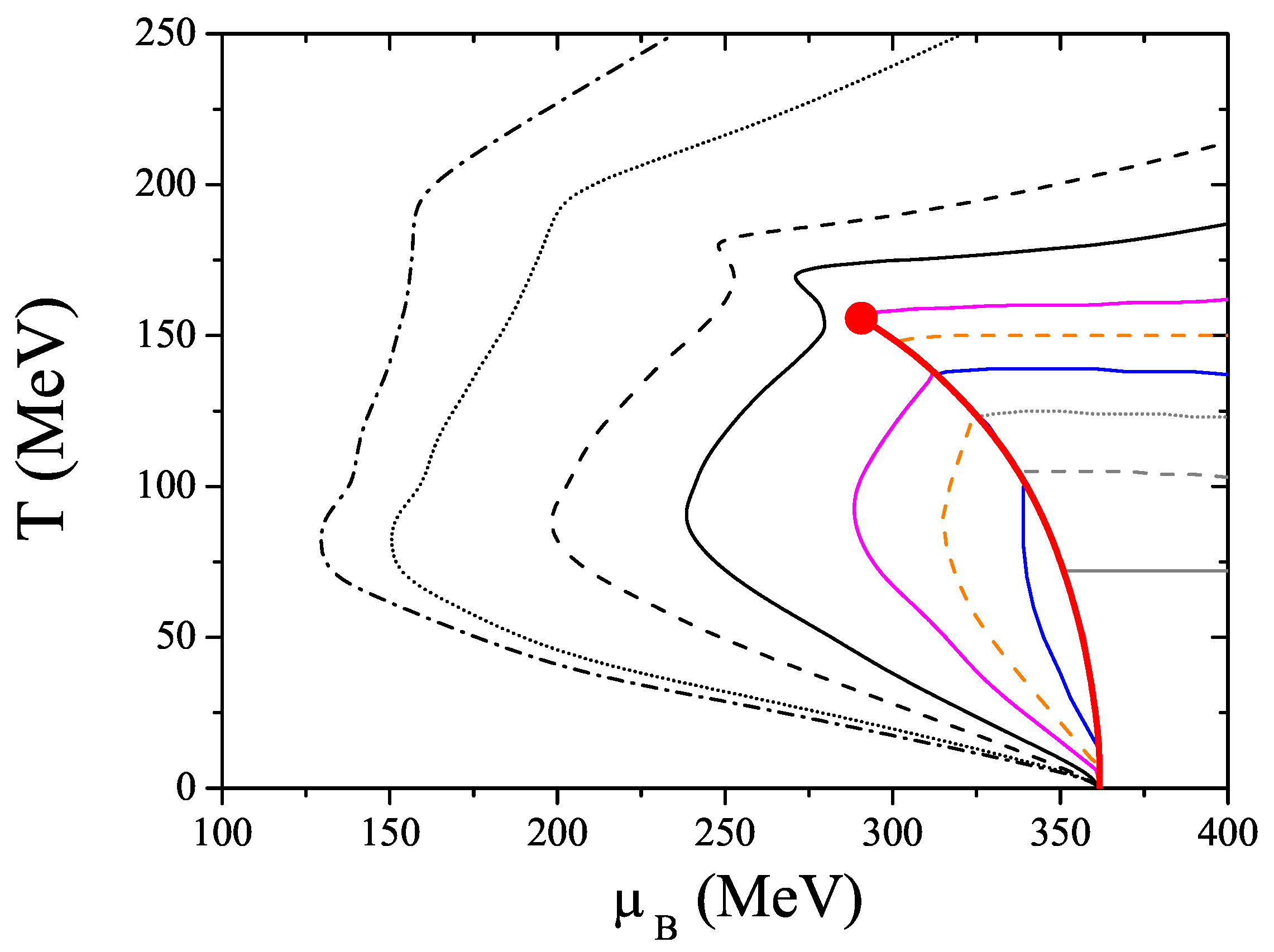
Our numerical results for the isentropic lines in the ( T , μ B ) plane are shown in Figure 7. We start the discussion by analyzing the behavior of the isentropic lines in the limit T 0 . As already analyzed in Section 5, our convenient choice of the model parameters allows a better description of the first order transition than other treatments of the NJL (PNJL) model. This choice is crucial to obtain important results: the criterion of stability of the quark droplets [36,109] is fulfilled, and, in addition, simple thermodynamic expectations in the limit T 0 are verified. In fact, in this limit s 0 according to the third law of thermodynamics and, as ρ B 0 too, the satisfaction of the condition s / ρ B = c o n s t . is insured. We recall (Section 5) that, at T = 0 , we are in the presence of droplets (states in mechanical equilibrium with the vacuum state ( ρ B = 0 ) at P = 0 ).
At T 0 , in the first order line, the behavior we find is somewhat different from those claimed by other authors [114,117] where a phenomena of focusing of trajectories towards the CEP is observed. We see that the isentropic lines with s / ρ B = 1 , . . . , 6 come from the region of symmetry partially restored and attain directly the phase transition; the trajectory s / ρ B = 1 goes along with the phase transition as T decreases until it reaches T = 0 ; and the other trajectories enter the hadronic phase where the symmetry is still broken and, after that, also converge to the horizontal axes ( T = 0 ). Consequently, even without reheating in the mixed phase as verified in the “zigzag” shape of [113,114,115,118], all isentropic trajectories directly terminate in the end of the first order transition line at T = 0 .
In the crossover region the behavior of the isentropic lines is qualitatively similar to the one obtained in lattice calculations [113] or in some models [114,115,119]. The trajectories with s / ρ B > 6 go directly to the crossover region and display a smooth behavior, although those that pass in the neighborhood of the CEP show a slightly kink behavior.
In conclusion, all the trajectories directly terminate in the same point of the horizontal axes at T = 0 . As already pointed out in [112], the picture provided here is a natural result in these type of quark models with no change in the number of degrees of freedom of the system in the two phases. As the temperature decreases a first order phase transition occurs, the latent heat increases and the formation of the mixed phase is thermodynamically favored.
We point out again that, in the limit T 0 , it is verified that s 0 and ρ B 0 , as it should be. This behavior is in contrast to the one reported in [112] (see right panel of Fig. 9 therein), where the NJL model in the SU(2) sector is used. The difference is due to our more convenient choice of the model parameters, mainly a lower value of the cutoff. This can be explained by the presence of droplets at T = 0 whose stability is quite sensitive to the choice of the model parameters.

7. Effects of Strangeness and Anomaly Strength on the Critical End Point

As already noticed, an important question which emerges in the study of the QCD phase diagram is whether the hadronic phase and the quark gluon like phase are separated by a phase transition in the thermodynamical sense. The identification of possible critical points associated to the phase transition is a challenging problem. Since we are working within a model with (2+1) flavors with the U A (1) anomaly included, we can explore new scenarios with regards to the usual SU(2) model without explicit anomaly. We have now two more parameters: the strange current quark mass, m s , and the anomaly coupling strength, g D , and it is certainly interesting to study the effect on thermodynamic quantities of changing these parameters. The anomaly is present via the ’t Hooft interaction and its effects appear explicitly in the gap equations (18) and in the expression of the thermodynamical potential (19) through products of the anomaly coefficient by quark condensates. Here we will discuss the influence on the location and the nature of the critical points of the degree of explicit symmetry breaking of both chiral symmetry (in the strange sector) and axial U A (1) symmetry.

7.1. Role of the Strangeness in the Location of the CEP/TCP

Let us study the influence of the strangeness in the location of the CEP/TCP. As we have already seen, the location of the CEP is found at T C E P = 155 . 80 MeV and μ B C E P = 290 . 67 MeV ( ρ B C E P = 1 . 87 ρ 0 ) when we use physical values of the quark masses [95,120]: m u = m d = 5 . 5 MeV, m s = 140 . 7 MeV.
A first point to be noticed is that in the PNJL model, contrarily to what happens in the chiral limit only for the SU(2) sector ( m u = m d = 0 , m s 0 ) where the TCP is found [76], when the total chiral limit is considered ( m u = m d = m s = 0 ), the phase diagram does not exhibit a TCP: chiral symmetry is restored via a first order transition for all baryonic chemical potentials and temperatures (see left panel of Figure 8). Both situations are in agreement with what is expected: the chiral phase transition at the chiral limit is of second order for N f = 2 and first order for N f 3 [121].
To study the influence of strangeness on the location of the critical points, we vary the current quark mass m s , keeping the SU(2) sector in the chiral limit and the other model parameters fixed. The phase diagram is presented in Figure 8 (right panel) as a function of μ B and T, and we consider different cases for the current quark mass m s .
The pattern of chiral symmetry restoration via first order phase transition remains for m u = m d = 0 and m s < m s c r i t [122]. The value for m s c r i t is a subject of debate; those found in lattice [123] or in model calculations [122,124] are lower than the physical strange current quark mass ( m s 150 MeV). We found m s c r i t 9 MeV in our model, lower than lattice values [123] and half of the value obtained in NJL model ( m s c r i t = 18 . 3 MeV [120]), but still consistent with other models of this type [124]. When m s m s c r i t , at μ B = 0 , the transition is of the second order and, as μ B increases, the line of the second order phase transition will end in a first order line at the TCP. Several TCPs are plotted for different values of m s in the right panel of Figure 8. As m s increases, the value of T for this “line” of TCPs decreases as μ B increases getting closer to the CEP and, when m s = 140 . 7 MeV, it starts to move away from the CEP. The TCP for m s = 140 . 7 MeV is the closest to the CEP and is located at μ B T C P = 206 . 95 MeV and T T C P = 187 . 83 MeV. If we choose m u = m d 0 , instead of a second order transition we have a smooth crossover for all the values of m s and the “line” of TCPs becomes a “line” of CEPs.

7.2. Role of the Anomaly Strength in the Location of the CEP

The axial U A (1) symmetry is broken explicitly by instantons, leaving a SU(N f ) × SU(N f ) symmetry which determines the chiral dynamics. Since instantons are screened in a hot or dense environment, the U A (1) symmetry may be effectively restored in matter. So, it is instructive to review this enlargement of chiral symmetry to SU(N f ) × SU(N f ) × U A (1) in more detail.
As already referred, the location and even the existence of the CEP in the phase diagram is a matter of debate [51]. While different lattice calculations predict the existence of a CEP [125], the absence of the CEP in the phase diagram was seen in recent lattice QCD results [79,80,81], where the first order phase transition region near μ B = 0 shrinks in the quark mass and μ B space when μ B is increased [79,80,81]. Due to the importance of the U A (1) anomaly, already emphasized in Section 2, and its influence on several observables, it is demanding to investigate possible changes in the location of the CEP in the ( T , μ B ) plane when the anomaly strength is modified. In Figure 9 we show the location of the CEP for several values of g D compared to the results for g D 0 , the value used for the vacuum. As already pointed out by K. Fukushima in [70], we also observe that the location of the CEP depends on the value of g D and, when g D is about 50% of its value in the vacuum, the QCD critical point disappears from the phase diagram; the first order region becomes narrower with the decreasing of the g D value.
The results show that, in the framework of this model, the existence or not of the CEP is determined by the strength of the anomaly coupling, the CEP getting closer to the μ B axis as g D decreases.

8. Susceptibilities and Critical Behavior in the Vicinity of the CEP

In the last years, the phenomenological relevance of fluctuations in the finite temperature and chemical potential around the CEP/TCP of QCD has been attracting the attention of several authors [126]. As a matter of fact, fluctuations are supposed to represent signatures of phase transitions of strongly interacting matter. In particular, the quark number susceptibility plays a role in the calculation of event-by-event fluctuations of conserved quantities such as the net baryon number. Across the quark hadron phase transition they are expected to become large; that can be interpreted as an indication for a critical behavior. We also remember the important role of the second derivative of the pressure for second order points like the CEP.
The grand canonical potential (or the pressure) contains the relevant information on thermodynamic bulk properties of a medium. Susceptibilities, being second order derivatives of the pressure in both chemical potential and temperature directions, are related to those fluctuations. The relevance of these physical observables is related with the size of the critical region around the CEP which can be found by calculating the specific heat, the baryon number susceptibility, and their critical behaviors. The size of this critical region is important for future searches of the CEP in heavy ion-collisions [114].
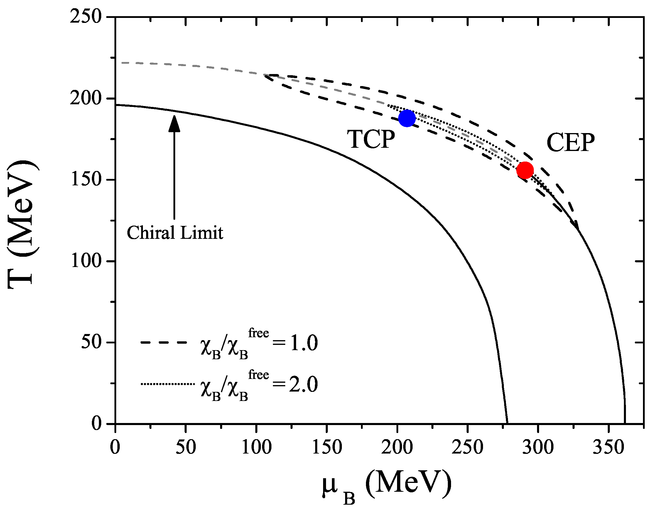
The way to estimate the critical region around the CEP is to calculate the dimensionless ratio χ B / χ B f r e e , where χ B f r e e is the chiral susceptibility of a free massless quark gas. Figure 10 shows a contour plot for two fixed ratios χ B / χ B f r e e = 1 . 0 and 2 . 0 in the phase diagram around the CEP. In the direction parallel to the first order transition line and to the crossover, it can be seen an elongation of the region where χ B is enhanced, indicating that the critical region is heavily stretched in that direction. It means that the divergence of the correlation length at the CEP affects the phase diagram quite far from the CEP and a careful analysis including effects beyond the mean-field needs to be done [127].
One of the main effects of the Polyakov loop is to shorten the temperature range where the crossover occurs [44]. On the other hand, this behavior is boosted by the choice of the regularization ( Λ ) [76]. The combination of both effects results in higher baryonic susceptibilities even far from the CEP when compared with the NJL model [128]. This effect of the Polyakov loop is driven by the fact that the one- and two-quark Boltzmann factors are controlled by a factor proportional to Φ : at small temperature Φ 0 results in a suppression of these contributions (see Equation (19)) leading to a partial restoration of the color symmetry. Indeed, the fact that only the 3 quark Boltzmann factors e 3 β E p contribute to the thermodynamical potential at low temperature, may be interpreted as the production of a thermal bath containing only colorless 3-quark contributions. When the temperature increases, Φ goes quickly to 1 resulting in a (partial) restoration of the chiral symmetry occurring in a shorter temperature range. The crossover taking place in a smaller T range can be interpreted as a crossover transition closest to a second order one. This “faster” crossover may explain the elongation of the critical region giving raise to a greater correlation length even far from the CEP.
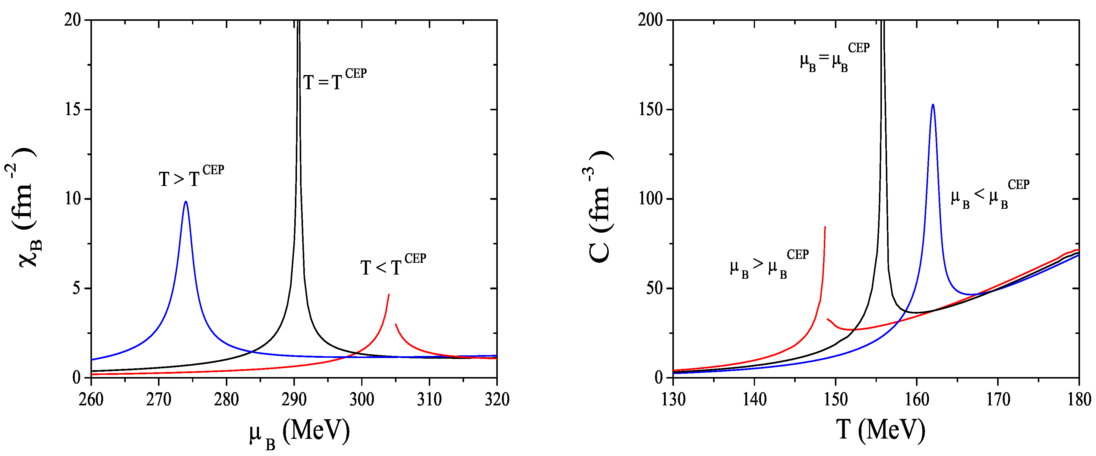
Now we show in Figure 11 the behavior of the baryon number susceptibility, χ B , and the specific heat, C, at the CEP, which is in accordance with [120,126,129].
The baryon number susceptibility is plotted (left panel) as a function of the baryon chemical potential for three values of the temperature. The divergent behavior of χ B at the CEP is an indication of the second order phase transition at this point. The curve for T > T C E P corresponds to the crossover and the other to the first order transition.
Now we will pay attention to the specific heat (Equation (27)) which is plotted as a function of the temperature around the CEP (right panel). The divergent behavior is the signal of the location of the CEP. The curve μ B < μ B C E P corresponds to the crossover and the other to the first order transition.
The large enhancement of the baryon number susceptibility and the specific heat at the CEP may be used as a signal of the existence and identification of phase transitions in the quark matter.

9. Conclusions

The concept of symmetries is a very important topic in physics. It has given a fruitful insight into the relationships between different areas, and has contributed to the unification of several phenomena, as shown in recent achievements in nuclear and hadronic physics.
Critical phenomena in hot QCD have been studied in the framework of the PNJL model, as an important issue to determine the order of the chiral phase transition as a function of the temperature and the quark chemical potential. Symmetry arguments show that the phase transition should be a first order one in the chiral limit ( m u = m d = m s = 0 ) . Working out of the chiral limit, at which both chiral and center symmetries are explicitly broken, a CEP which separates first and crossover lines is found, and the corresponding order parameters are analyzed.
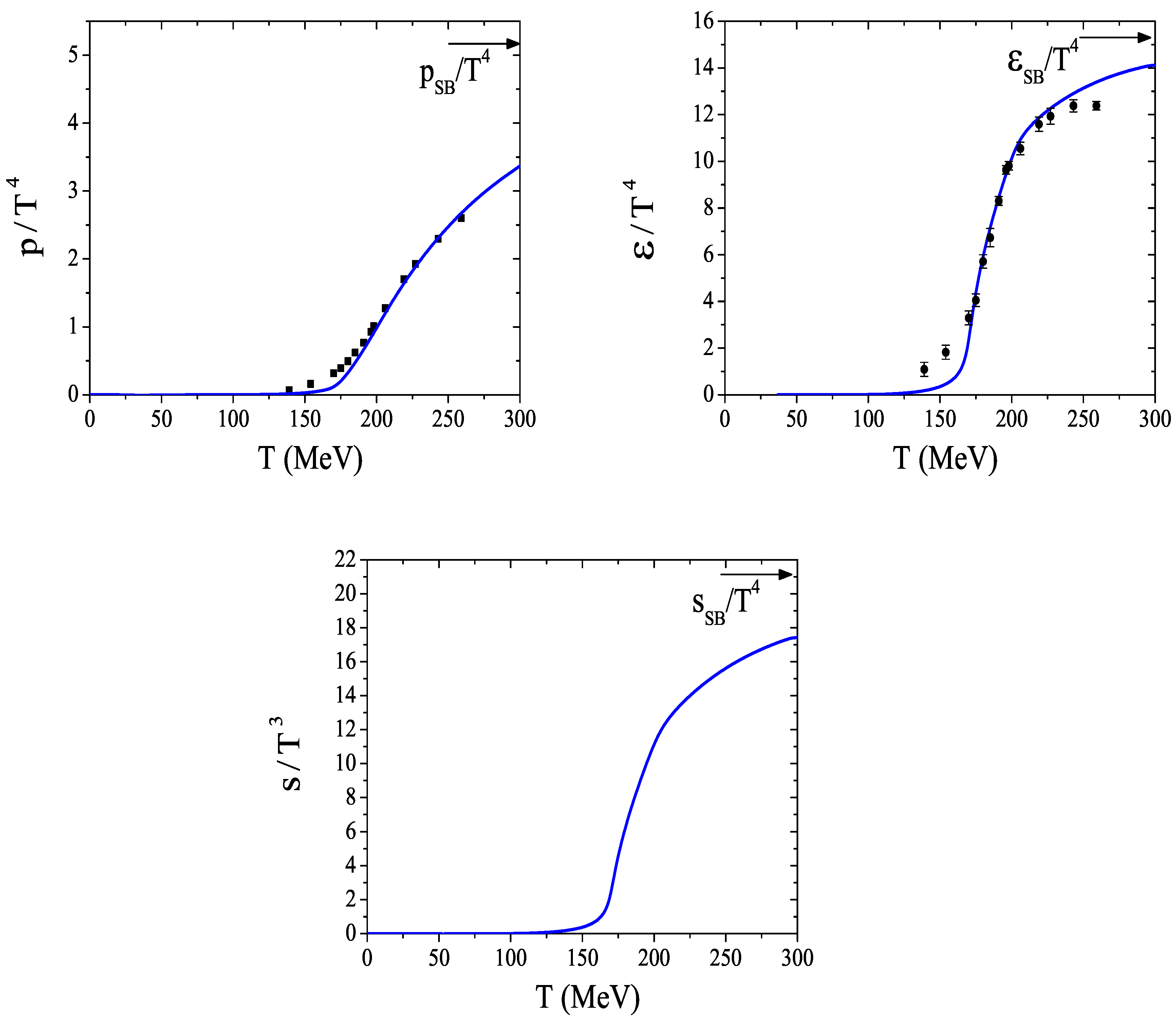
The sets of parameters used is compatible with the formation of stable droplets at zero temperature, insuring the satisfaction of important thermodynamic expectations like the Nernst principle. Other important role is played by the regularization procedure which, by allowing high momentum quark states, is essential to obtain the required increase of extensive thermodynamic quantities, insuring the convergence to the Stefan–Boltzmann (SB) limit of QCD. In this context the gluonic degrees of freedom also play a special role.
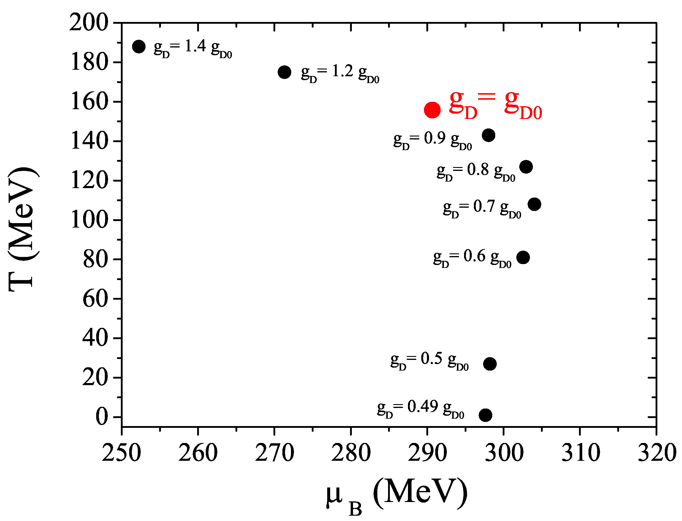
We also discussed the effect of the U A (1) axial symmetry both at zero and at finite temperature. We analyzed the effect of the anomalous coupling strength in the location of the CEP. We proved that the location of the CEP depends on the value of g D and, when g D is about 50% of its value in the vacuum, the QCD critical point disappears from the phase diagram. One expects that, above a certain critical temperature T e f f , the chiral and axial symmetries will be effectively restored. The behavior of some given observables signals the effective restoration of these symmetries: for instance, the topological susceptibility vanishes.
The successful comparison with lattice results shows that the model calculation provides a convenient tool to obtain information for systems from zero to non-zero chemical potential which is of particular importance for the knowledge of the equation of state of hot and dense matter. Although the results here presented relies on the chiral/deconfinement phase transition, the relevant physics involved is also useful to understand other phase transitions sharing similar features.

Acknowledgements

Work supported by Centro de Física Computacional and F.C.T. under Project No. CERN/FP/83644/2008.

Appendix

The quark condensates q i ¯ q i , with i , j , k = u , d , s (to be fixed in cyclic order), determined in a self-consistent way, are given by:
q ¯ i q i = 2 N c d 3 p 2 π 3 M i E i [ θ ( Λ 2 p 2 ) f Φ ( + ) ( E i ) f Φ ( ) ( E i ) ]
where E i is the quasi-particle energy for the quark i: E i = p 2 + M i 2 .
All calculations in the NJL model can be generalized to the PNJL one, as was shown in [44], by introducing the modified Fermi-Dirac distribution functions for particles and antiparticles used in the expression of q ¯ i q i :
f Φ ( + ) ( E i ) = Φ ¯ e β E p + 2 Φ e 2 β E p + e 3 β E p exp { z Φ + ( E i ) }
f Φ ( ) ( E i ) = Φ e β E p + + 2 Φ ¯ e 2 β E p + + e 3 β E p + exp { z Φ ( E i ) }
The mean field equations are obtained by minimizing the thermodynamical potential density (19) with respect to q ¯ i q i ( i = u , d , s ), Φ , and Φ ¯ . The respective mean field equations are the already given gap equation (18) and
0 = T 4 a ( T ) 2 Φ ¯ 6 b ( T ) Φ ¯ 2 Φ 2 + Φ ¯ 2 Φ 1 6 Φ ¯ Φ + 4 ( Φ ¯ 3 + Φ 3 ) 3 ( Φ ¯ Φ ) 2 6 T i = u , d , s d 3 p 2 π 3 e 2 β E p exp { z Φ + ( E i ) } + e β E p + exp { z Φ ( E i ) }
0 = T 4 a ( T ) 2 Φ 6 b ( T ) Φ 2 Φ ¯ 2 + Φ ¯ Φ 2 1 6 Φ ¯ Φ + 4 ( Φ ¯ 3 + Φ 3 ) 3 ( Φ ¯ Φ ) 2 6 T i = u , d , s d 3 p 2 π 3 e β E p exp { z Φ + ( E i ) } + e 2 β E p + exp { z Φ ( E i ) }

References

  1. Nambu, Y. Axial vector current conservation in weak interactions. Phys. Rev. Lett. 1960, 4, 380–382. [Google Scholar] [CrossRef]
  2. Leutwyler, H. Strong interactions at low energies. Czech. J. Phys. 2002, 52, B9–B27. [Google Scholar] [CrossRef]
  3. Weinberg, S. Phenomenological Lagrangians. Physica 1979, A96, 327. [Google Scholar] [CrossRef]
  4. Gasser, J.; Leutwyler, H. Chiral perturbation theory: Expansions in the mass of the strange quark. Nucl. Phys. 1985, B250, 465. [Google Scholar] [CrossRef]
  5. Nambu, Y.; Jona-Lasinio, G. Dynamical model of elementary particles based on an analogy with superconductivity. I. Phys. Rev. 1961, 122, 345–358. [Google Scholar] [CrossRef]
  6. Nambu, Y.; Jona-Lasinio, G. Dynamical model of elementary particles based on an analogy with superconductivity. II. Phys. Rev. 1961, 124, 246–254. [Google Scholar] [CrossRef]
  7. Eguchi, T. A new approach to collective phenomena in superconductivity models. Phys. Rev. 1976, D14, 2755. [Google Scholar] [CrossRef]
  8. Kikkawa, K. Quantum corrections in superconductor models. Prog. Theor. Phys. 1976, 56, 947. [Google Scholar] [CrossRef]
  9. Volkov, M.K.; Ebert, D. Four-quark interactions as a common source of the vector meson dominance and Sigma model. (in Russian). Yad. Fiz. 1982, 36, 1265–1277. [Google Scholar]
  10. Ebert, D.; Volkov, M.K. Composite Meson Model with Vector Dominance Based on U(2) Invariant Four Quark Interactions. Z. Phys. 1983, C16, 205. [Google Scholar] [CrossRef]
  11. Volkov, M.K. Meson Lagrangians in a Superconductor Quark Model. Annals Phys. 1984, 157, 282–303. [Google Scholar] [CrossRef]
  12. Volkov, M.K.; Radzhabov, A.E. Forty-fifth anniversary of the Nambu–Jona-Lasinio model. arXiv:hep-ph/0508263.
  13. Mannarelli, M.; Rapp, R. Hadronic modes and quark properties in the quark-gluon plasma. Phys. Rev. 2005, C72, 064905. [Google Scholar] [CrossRef]
  14. Kitazawa, M.; Kunihiro, T.; Nemoto, Y. Quark spectrum above but near critical temperature of chiral transition. Phys. Lett. 2006, B633, 269–274. [Google Scholar] [CrossRef]
  15. Datta, S.; Karsch, F.; Petreczky, P.; Wetzorke, I. Behavior of charmonium systems after deconfinement. Phys. Rev. 2004, D69, 094507. [Google Scholar] [CrossRef]
  16. Shuryak, E.V.; Zahed, I. Towards a theory of binary bound states in the quark gluon plasma. Phys. Rev. 2004, D70, 054507. [Google Scholar] [CrossRef]
  17. Shuryak, E.V. What RHIC experiments and theory tell us about properties of quark-gluon plasma? Nucl. Phys. 2005, A750, 64–83. [Google Scholar] [CrossRef]
  18. Wong, C.Y. Heavy quarkonia in quark gluon plasma. Phys. Rev. 2005, C72, 034906. [Google Scholar] [CrossRef]
  19. Wong, C.Y. Quarkonia and quark drip lines in quark-gluon plasma. Phys. Rev. 2007, C76, 014902. [Google Scholar] [CrossRef]
  20. Datta, S.; Karsch, F.; Petreczky, P.; Wetzorke, I. Meson correlators above deconfinement. J. Phys. 2005, G31, S351–S356. [Google Scholar] [CrossRef]
  21. Alberico, W.M.; Beraudo, A.; De Pace, A.; Molinari, A. Heavy quark bound states above Tc. Phys. Rev. 2005, D72, 114011. [Google Scholar]
  22. Mocsy, A.; Petreczky, P. Quarkonia correlators above deconfinement. Phys. Rev. 2006, D73, 074007. [Google Scholar] [CrossRef]
  23. Koch, V.; Majumder, A.; Randrup, J. Baryon-strangeness correlations: A diagnostic of strongly interacting matter. Phys. Rev. Lett. 2005, 95, 182301. [Google Scholar] [CrossRef]
  24. Ejiri, S.; Karsch, F.; Redlich, K. Hadronic fluctuations at the QCD phase transition. Phys. Lett. 2006, B633, 275–282. [Google Scholar] [CrossRef]
  25. Liao, J.; Shuryak, E.V. What do lattice baryonic susceptibilities tell us about quarks, diquarks and baryons at T > Tc. Phys. Rev. 2006, D73, 014509. [Google Scholar] [CrossRef]
  26. De Forcrand, P.; Garcia Perez, M.; Hashimoto, T.; Hioki, S.; Matsufuru, H.; Miyamura, O.; Nakamura, A.; Stamatescu, I.-O.; Takaishi, T.; Umeda, T. Mesons above the deconfining transition. 1999; arXiv:hep-lat/9901017v3. [Google Scholar]
  27. Pushkina, I.; de Forcrand, P.; Prez-Garcia, M.; Kim, S.; Matsufuru, H.; Nakamura, A.; Stamatescu, I.O.; Takaishi, T.; Umeda, T. Properties of hadron screening masses at finite baryonic density. Phys. Lett. 2005, B609, 265–270. [Google Scholar] [CrossRef]
  28. Petreczky, P. Lattice calculations of meson correlators and spectral functions at finite temperature. J. Phys. 2004, G30, S431–S440. [Google Scholar] [CrossRef]
  29. Wissel, S.; Laermann, E.; Shcheredin, S.; Datta, S.; Karsch, F. Meson correlation functions at high temperatures. PoS 2006, LAT2005, 164. [Google Scholar]
  30. Hansson, T.H.; Zahed, I. Hadronic correlators in hot QCD. Nucl. Phys. 1992, B374, 277–287. [Google Scholar] [CrossRef]
  31. Laine, M.; Vepsalainen, M. Mesonic correlation lengths in high-temperature QCD. JHEP 2004, 02, 004. [Google Scholar] [CrossRef]
  32. Alberico, W.M.; Beraudo, A.; Molinari, A. Meson correlation functions in a QCD plasma. Nucl. Phys. 2005, A750, 359–390. [Google Scholar] [CrossRef]
  33. Alberico, W.M.; Beraudo, A.; Czerski, P.; Molinari, A. Finite momentum meson correlation functions in a QCD plasma. Nucl. Phys. 2006, A775, 188–211. [Google Scholar] [CrossRef]
  34. Karsch, F.; Mustafa, M.G.; Thoma, M.H. Finite temperature meson correlation functions in HTL approximation. Phys. Lett. 2001, B497, 249–258. [Google Scholar] [CrossRef]
  35. Klevansky, S.P. The Nambu–Jona-Lasinio model of quantum chromodynamics. Rev. Mod. Phys. 1992, 64, 649–708. [Google Scholar] [CrossRef]
  36. Buballa, M. NJL model analysis of quark matter at large density. Phys. Rept. 2005, 407, 205–376. [Google Scholar] [CrossRef]
  37. Meisinger, P.N.; Ogilvie, M.C. Chiral symmetry restoration and ZN symmetry. Phys. Lett. 1996, B379, 163–168. [Google Scholar] [CrossRef]
  38. Pisarski, R.D. Quark-gluon plasma as a condensate of SU(3) Wilson lines. Phys. Rev. 2000, D62, 111501. [Google Scholar]
  39. Pisarski, R.D. Notes on the deconfining phase transition. 2002; arXiv:hep-ph/0203271. [Google Scholar]
  40. Meisinger, P.N.; Miller, T.R.; Ogilvie, M.C. Phenomenological equations of state for the quark-gluon plasma. Phys. Rev. 2002, D65, 034009. [Google Scholar]
  41. Fukushima, K. Chiral effective model with the Polyakov loop. Phys. Lett. 2004, B591, 277–284. [Google Scholar] [CrossRef]
  42. Mocsy, A.; Sannino, F.; Tuominen, K. Confinement versus Chiral Symmetry. Phys. Rev. Lett. 2004, 92, 182302. [Google Scholar] [CrossRef] [PubMed]
  43. Ratti, C.; Thaler, M.A.; Weise, W. Phases of QCD: Lattice thermodynamics and a field theoretical model. Phys. Rev. 2006, D73, 014019. [Google Scholar] [CrossRef]
  44. Hansen, H.; Alberico, W.M.; Beraudo, A.; Molinari, A.; Nardi, M.; Ratti, C. Mesonic correlation functions at finite temperature and density in the Nambu-Jona-Lasinio model with a Polyakov loop. Phys. Rev. 2007, D75, 065004. [Google Scholar]
  45. Asakawa, M.; Yazaki, K. Chiral restorations at finite density and temperature. Nucl. Phys. 1989, A504, 668–684. [Google Scholar]
  46. Barducci, A.; Casalbuoni, R.; De Curtis, S.; Gatto, R.; Pettini, G. Chiral symmetry breaking in QCD at finite temperature and density. Phys. Lett. 1989, B231, 463. [Google Scholar] [CrossRef]
  47. Barducci, A.; Casalbuoni, R.; De Curtis, S.; Gatto, R.; Pettini, G. Chiral Phase transitions in QCD for finite temperature and density. Phys. Rev. 1990, D41, 1610. [Google Scholar] [CrossRef]
  48. Barducci, A.; Casalbuoni, R.; Pettini, G.; Gatto, R. Chiral phases of QCD at finite density and temperature. Phys. Rev. 1994, D49, 426–436. [Google Scholar] [CrossRef]
  49. Stephanov, M.A. QCD phase diagram and the critical point. Prog. Theor. Phys. Suppl. 2004, 153, 139–156. [Google Scholar] [CrossRef]
  50. Casalbuoni, R. QCD critical point: A historical perspective. PoS 2006, CPOD2006, 001. [Google Scholar]
  51. Casalbuoni, R. 5th International Workshop on Critical Point and Onset of Deconfinement. PoS 2009, CPOD 2009. [Google Scholar]
  52. Weinberg, S. Nonabelian Gauge Theories of the Strong Interactions. Phys. Rev. Lett. 1973, 31, 494–497. [Google Scholar] [CrossRef]
  53. Fritzsch, H.; Gell-Mann, M.; Leutwyler, H. Advantages of the Color Octet Gluon Picture. Phys. Lett. 1973, B47, 365–368. [Google Scholar] [CrossRef]
  54. ’t Hooft, G. Renormalization of Massless Yang-Mills Fields. Nucl. Phys. 1971, B33, 173–199. [Google Scholar]
  55. Gross, D.J.; Wilczek, F. Ultraviolet Behavior of Non-Abelian Gauge Theories. Phys. Rev. Lett. 1973, 30, 1343–1346. [Google Scholar] [CrossRef]
  56. Politzer, H.D. Reliable Perturbative Results for Strong Interactions? Phys. Rev. Lett. 1973, 30, 1346–1349. [Google Scholar] [CrossRef]
  57. Goldstone, J. Field Theories with Superconductor Solutions. Nuovo Cim. 1961, 19, 154–164. [Google Scholar] [CrossRef]
  58. Goldstone, J.; Salam, A.; Weinberg, S. Broken Symmetries. Phys. Rev. 1962, 127, 965–970. [Google Scholar] [CrossRef]
  59. Hatsuda, T.; Kunihiro, T. QCD phenomenology based on a chiral effective Lagrangian. Phys. Rept. 1994, 247, 221–367. [Google Scholar] [CrossRef]
  60. Weinberg, S. The U(1) problem. Phys. Rev. 1975, D11, 3583–3593. [Google Scholar] [CrossRef]
  61. ’t Hooft, G. Symmetry breaking through Bell-Jackiw anomalies. Phys. Rev. Lett. 1976, 37, 8–11. [Google Scholar] [CrossRef]
  62. ’t Hooft, G. Computation of the quantum effects due to a four- dimensional pseudoparticle. Phys. Rev. 1976, D14, 3432–3450. [Google Scholar] [CrossRef]
  63. Polyakov, A.M. Thermal properties of gauge fields and quark liberation. Phys. Lett. 1978, B72, 477–480. [Google Scholar] [CrossRef]
  64. ’t Hooft, G. On the phase transition towards permanent quark confinement. Nucl. Phys. 1978, B138, 1. [Google Scholar] [CrossRef]
  65. Svetitsky, B.; Yaffe, L.G. Critical behavior at finite temperature confinement transitions. Nucl. Phys. 1982, B210, 423. [Google Scholar] [CrossRef]
  66. McLerran, L.D.; Svetitsky, B. Quark Liberation at High Temperature: A Monte Carlo Study of SU(2) Gauge Theory. Phys. Rev. 1981, D24, 450. [Google Scholar] [CrossRef]
  67. Rothe, H.J. Lattice gauge theories: An Introduction. World Sci. Lect. Notes Phys. 2005, 74, 1–605. [Google Scholar]
  68. Ratti, C.; Thaler, M.A.; Weise, W. Phase diagram and thermodynamics of the PNJL model. 2006; arXiv:nucl-th/0604025. [Google Scholar]
  69. Roessner, S.; Ratti, C.; Weise, W. Polyakov loop, diquarks and the two-flavor phase diagram. Phys. Rev. 2007, D75, 034007. [Google Scholar]
  70. Fukushima, K. Phase diagrams in the three-flavor Nambu–Jona-Lasinio model with the Polyakov loop. Phys. Rev. 2008, D77, 114028. [Google Scholar] [CrossRef]
  71. Sasaki, C.; Friman, B.; Redlich, K. Susceptibilities and the phase structure of a chiral model with Polyakov loops. Phys. Rev. 2007, D75, 074013. [Google Scholar] [CrossRef]
  72. Sasaki, C.; Friman, B.; Redlich, K. Quark number fluctuations in a chiral model at finite baryon chemical potential. Phys. Rev. 2007, D75, 054026. [Google Scholar] [CrossRef]
  73. Kaczmarek, O.; Karsch, F.; Petreczky, P.; Zantow, F. Heavy quark anti-quark free energy and the renormalized Polyakov loop. Phys. Lett. 2002, B543, 41–47. [Google Scholar] [CrossRef]
  74. Kaczmarek, O. Screening at finite temperature and density. PoS 2007, CPOD07, 043. [Google Scholar]
  75. Schaefer, B.J.; Pawlowski, J.M.; Wambach, J. The Phase Structure of the Polyakov–Quark-Meson Model. Phys. Rev. 2007, D76, 074023. [Google Scholar] [CrossRef]
  76. Costa, P.; Hansen, H.; Ruivo, M.C.; de Sousa, C.A. How parameters and regularization affect the PNJL model phase diagram and thermodynamic quantities. Phys. Rev. 2010, D81, 016007. [Google Scholar]
  77. Cheng, M.; Ejiri, S.; Hegde, P.; Karsch, F.; Kaczmarek, O.; Laermann, E.; Mawhinney, R.D.; Miao, C.; Mukherjee, S.; Petreczky, P.; Schmidt, C.; Soeldner, W. Equation of State for physical quark masses. Phys. Rev. 2010, D81, 054504. [Google Scholar] [CrossRef]
  78. Adams, J.; Aggarwal, M.M.; Ahammed, Z.; Amonett, J.; Anderson, B.D.; Arkhipkin, D.; Averichev, G.S.; Badyal, S.K.; Bai, Y.; Balewski, J.; et al. Experimental and theoretical challenges in the search for the quark gluon plasma: The STAR collaboration’s critical assessment of the evidence from RHIC collisions. Nucl. Phys. 2005, A757, 102–183. [Google Scholar] [CrossRef]
  79. De Forcrand, P.; Philipsen, O. The chiral critical line of Nf = 2 + 1 QCD at zero and non- zero baryon density. JHEP 2007, 01, 077. [Google Scholar] [CrossRef]
  80. De Forcrand, P.; Kim, S.; Philipsen, O. A QCD chiral critical point at small chemical potential: is it there or not? PoS 2007, LAT2007, 178. [Google Scholar]
  81. De Forcrand, P.; Philipsen, O. The chiral critical point of Nf = 3 QCD at finite density to the order (μ/T)4. JHEP 2008, 11, 012. [Google Scholar] [CrossRef]
  82. Antoniou, N.G.; Diakonos, F.K.; Mavromanolakis, G.; Anticic, T.; Baatar, B.; Barna, D.; Bartke, J.; Betev, L.; Bialkowska, H.; Blume, C.; et al. Search for the QCD critical point in nuclear collisions at the CERN SPS. Phys. Rev. 2010, D81, 054504. [Google Scholar]
  83. Alford, M.G.; Schmitt, A.; Rajagopal, K.; Schafer, T. Color superconductivity in dense quark matter. Rev. Mod. Phys. 2008, 80, 1455–1515. [Google Scholar] [CrossRef]
  84. McLerran, L.; Pisarski, R.D. Phases of Cold, Dense Quarks at Large Nc. Nucl. Phys. 2007, A796, 83–100. [Google Scholar] [CrossRef]
  85. Hidaka, Y.; McLerran, L.D.; Pisarski, R.D. Baryons and the phase diagram for a large number of colors and flavors. Nucl. Phys. 2008, A808, 117–123. [Google Scholar] [CrossRef]
  86. McLerran, L.; Redlich, K.; Sasaki, C. Quarkyonic Matter and Chiral Symmetry Breaking. Nucl. Phys. 2009, A824, 86–100. [Google Scholar] [CrossRef]
  87. Andronic, A.; Blaschke, D.; Braun-Munzinger, P.; Cleymans, J.; Fukushima, K.; McLerran, L.D.; Oeschler, H.; Pisarski, R.D.; Redlich, K.; Sasaki, C.; Satz, H.; Stachel, J. Hadron Production in Ultra-relativistic Nuclear Collisions: Quarkyonic Matter and a Triple Point in the Phase Diagram of QCD. Nucl. Phys. 2010, A837, 65–86. [Google Scholar] [CrossRef]
  88. Adcox, K.; Adler, S.S.; Ajitanand, N.N.; Akiba, Y.; Alexander, J.; Aphecetche, L.; Arai, Y.; Aronson, S.H.; Averbeck, R.; Awes, T.C.; et al. Formation of dense partonic matter in relativistic nucleus nucleus collisions at RHIC: Experimental evaluation by the PHENIX collaboration. Nucl. Phys. 2005, A757, 184–283. [Google Scholar] [CrossRef]
  89. Braun-Munzinger, P.; Stachel, J. The quest for the quark-gluon plasma. Nature 2007, 448, 302–309. [Google Scholar] [CrossRef] [PubMed]
  90. Hohne, C. The compressed baryonic matter experiment at the future accelerator facility in Darmstadt. Nucl. Phys. 2005, A749, 141–149. [Google Scholar] [CrossRef]
  91. Sissakian, A.; Sorin, A. NICA targets the mixed phase in hadron matter. CERN Cour. 2010, 50N1, 13–15. [Google Scholar]
  92. Cleymans, J.; Oeschler, H.; Redlich, K.; Wheaton, S. Comparison of chemical freeze-out criteria in heavy-ion collisions. Phys. Rev. 2006, C73, 034905. [Google Scholar] [CrossRef]
  93. Brockmann, R.; Weise, W. The Chiral condensate in nuclear matter. Phys. Lett. 1996, B367, 40–44. [Google Scholar] [CrossRef]
  94. Vogl, U.; Weise, W. The Nambu and Jona Lasinio model: Its implications for hadrons and nuclei. Prog. Part. Nucl. Phys. 1991, 27, 195–272. [Google Scholar] [CrossRef]
  95. Rehberg, P.; Klevansky, S.P.; Hufner, J. Hadronization in the SU(3) Nambu-Jona-Lasinio model. Phys. Rev. 1996, C53, 410–429. [Google Scholar] [CrossRef]
  96. Fu, W.J.; Zhang, Z.; Liu, Y.X. 2+1 Flavor Polyakov–Nambu–Jona-Lasinio Model at Finite Temperature and Nonzero Chemical Potential. Phys. Rev. 2008, D77, 014006. [Google Scholar]
  97. Ciminale, M.; Gatto, R.; Ippolito, N.D.; Nardulli, G.; Ruggieri, M. Three flavor Nambu–Jona Lasinio model with Polyakov loop and competition with nuclear matter. Phys. Rev. 2008, D77, 054023. [Google Scholar] [CrossRef]
  98. Meisinger, P.N.; Ogilvie, M.C.; Miller, T.R. Gluon quasiparticles and the Polyakov loop. Phys. Lett. 2004, B585, 149–154. [Google Scholar] [CrossRef]
  99. Costa, P.; Ruivo, M.C.; de Sousa, C.A. Effects of the regularization on the restoration of chiral and axial symmetries. Phys. Rev. 2008, D77, 096009. [Google Scholar] [CrossRef]
  100. Ruivo, M.C.; Costa, P.; de Sousa, C.A.; Hansen, H.; Alberico, W.M. How the Polyakov loop and the regularization affect strangeness and restoration of symmetries at finite T. 2010; arXiv:1001.3072. [Google Scholar]
  101. Alles, B.; D’Elia, M.; Di Giacomo, A. Topological susceptibility at zero and finite T in SU(3) Yang-Mills theory. Nucl. Phys. 1997, B494, 281–292. [Google Scholar] [CrossRef]
  102. Costa, P.; Ruivo, M.C.; de Sousa, C.A.; Hansen, H.; Alberico, W.M. Scalar-pseudoscalar meson behavior and restoration of symmetries in SU(3) PNJL model. Phys. Rev. 2009, D79, 116003. [Google Scholar]
  103. Megias, E.; Ruiz Arriola, E.; Salcedo, L.L. Polyakov loop in chiral quark models at finite temperature. Phys. Rev. 2006, D74, 065005. [Google Scholar] [CrossRef]
  104. Megias, E.; Ruiz Arriola, E.; Salcedo, L.L. Chiral Lagrangian at finite temperature from the Polyakov- Chiral Quark Model. Phys. Rev. 2006, D74, 114014. [Google Scholar] [CrossRef]
  105. Philipsen, O. Lattice QCD at finite temperature and density. Eur. Phys. J. ST 2007, 152, 29–60. [Google Scholar] [CrossRef]
  106. Blaschke, D.; Buballa, M.; Radzhabov, A.E.; Volkov, M.K. Effects of mesonic correlations in the QCD phase transition. Yad. Fiz. 2008, 71, 2012–2018. [Google Scholar] [CrossRef]
  107. Buballa, M.; Oertel, M. Quark droplets in the NJL mean field. Nucl. Phys. 1998, A642, 39–44. [Google Scholar] [CrossRef]
  108. Mishustin, I.N.; Satarov, L.M.; Stoecker, H.; Greiner, W. Unusual bound states of quark matter within the NJL model. Phys. Rev. 2000, C62, 034901. [Google Scholar]
  109. Costa, P.; Ruivo, M.C.; Kalinovsky, Y.L.; de Sousa, C.A. Pseudoscalar mesons in hot, dense matter. Phys. Rev. 2004, C70, 025204. [Google Scholar] [CrossRef]
  110. Rajagopal, K. Mapping the QCD phase diagram. Nucl. Phys. 1999, A661, 150–161. [Google Scholar] [CrossRef]
  111. Berges, J.; Rajagopal, K. Color superconductivity and chiral symmetry restoration at nonzero baryon density and temperature. Nucl. Phys. 1999, B538, 215–232. [Google Scholar] [CrossRef]
  112. Scavenius, O.; Mocsy, A.; Mishustin, I.N.; Rischke, D.H. Chiral phase transition within effective models with constituent quarks. Phys. Rev. 2001, C64, 045202. [Google Scholar] [CrossRef]
  113. Ejiri, S.; Karsch, F.; Laermann, E.; Schmidt, C. The isentropic equation of state of 2-flavor QCD. Phys. Rev. 2006, D73, 054506. [Google Scholar] [CrossRef]
  114. Nonaka, C.; Asakawa, M. Hydrodynamical evolution near the QCD critical end point. Phys. Rev. 2005, C71, 044904. [Google Scholar] [CrossRef]
  115. Kahara, T.; Tuominen, K. Degrees of freedom and the phase transitions of two flavor QCD. Phys. Rev. 2008, D78, 034015. [Google Scholar]
  116. Stephanov, M.A.; Rajagopal, K.; Shuryak, E.V. Signatures of the tricritical point in QCD. Phys. Rev. Lett. 1998, 81, 4816–4819. [Google Scholar] [CrossRef]
  117. Stephanov, M.A.; Rajagopal, K.; Shuryak, E.V. Event-by-event fluctuations in heavy ion collisions and the QCD critical point. Phys. Rev. 1999, D60, 114028. [Google Scholar]
  118. Subramanian, P.R.; Stoecker, H.; Greiner, W. Dynamics of the hadronization phase transition at finite baryon chemical potentials. Phys. Lett. 1986, B173, 468–472. [Google Scholar] [CrossRef]
  119. Fukushima, K. Isentropic thermodynamics in the PNJL model. Phys. Rev. 2009, D79, 074015. [Google Scholar]
  120. Costa, P.; de Sousa, C.A.; Ruivo, M.C.; Kalinovsky, Y.L. The QCD critical end point in the SU(3) Nambu–Jona-Lasinio model. Phys. Lett. 2007, B647, 431–435. [Google Scholar] [CrossRef]
  121. Pisarski, R.D.; Wilczek, F. Remarks on the chiral phase transition in chromodynamics. Phys. Rev. 1984, D29, 338–341. [Google Scholar] [CrossRef]
  122. Hsu, S.D.H.; Schwetz, M. On the QCD phase transition at finite baryon density. Phys. Lett. 1998, B432, 203–208. [Google Scholar] [CrossRef]
  123. Laermann, E.; Philipsen, O. Status of lattice QCD at finite temperature. Ann. Rev. Nucl. Part. Sci. 2003, 53, 163–198. [Google Scholar] [CrossRef]
  124. Barducci, A.; Casalbuoni, R.; Pettini, G.; Ravagli, L. A NJL-based study of the QCD critical line. Phys. Rev. 2005, D72, 056002. [Google Scholar]
  125. Fodor, Z.; Katz, S.D. Critical point of QCD at finite T and μ, lattice results for physical quark masses. JHEP 2004, 04, 050. [Google Scholar] [CrossRef]
  126. Hatta, Y.; Ikeda, T. Universality, the QCD critical / tricritical point and the quark number susceptibility. Phys. Rev. 2003, D67, 014028. [Google Scholar] [CrossRef]
  127. Roessner, S.; Hell, T.; Ratti, C.; Weise, W. The chiral and deconfinement crossover transitions: PNJL model beyond mean field. Nucl. Phys. 2008, A814, 118–143. [Google Scholar] [CrossRef]
  128. Costa, P.; de Sousa, C.A.; Ruivo, M.C.; Hansen, H. The QCD critical end point in the PNJL model. Europhys. Lett. 2009, 86, 31001. [Google Scholar] [CrossRef]
  129. Schaefer, B.J.; Wambach, J. Susceptibilities near the QCD (tri)critical point. Phys. Rev. 2007, D75, 085015. [Google Scholar] [CrossRef]
Figure 1. The phase diagram from the experimental point of view: freeze-out points for the different beam energies are showed [92].
Symmetry 02 01338 g001
Figure 2. Upper part: quark masses (left panel) and quark condensates (right panel) in PNJL model as functions of the temperature; the Polyakov loop field Φ is also shown. At T e f f = 345 MeV, M i = m i . Lower part: derivatives of the quark condensates and of the Polyakov loop field Φ (left panel); the topological susceptibility, χ , (right panel) in the PNJL model, compared to corresponding lattice results taken from [101].
Symmetry 02 01338 g002
Figure 3. Scaled pressure ( p ) , energy per particle ( ϵ ) , and entropy ( s ) as a function of the temperature at zero chemical potential. The data points are taken from [77]. The pressure reaches 66% of the strength of the Stefan-Boltzmann value at T = 300 MeV, a value which attains 85% at T = 400 MeV.
Symmetry 02 01338 g003
Figure 4. Left: grand potential for the stable, metastable and unstable phases, used to determine μ B c r and u quark mass; right: baryonic density as function of μ B .
Symmetry 02 01338 g004
Figure 5. Pressure (left) and energy per particle (right) as a function of ρ B / ρ 0 at different temperatures ( ρ 0 = 0 . 17 fm 3 is the normal nuclear matter density). The points A and B (left panel) illustrate the Gibbs criteria. Only in the T = 0 line the zero-pressure point is located at the minimum of the energy per particle.
Symmetry 02 01338 g005
Figure 6. Phase diagram in the SU(3) PNJL model. The left (right) part corresponds to the T μ B ( T ρ B ) plane. Solid (dashed) line shows the location of the first order (crossover) transition. The dashed lines shows the location of the spinodal boundaries of the two phase transitions (shown by shading in the right plot).
Symmetry 02 01338 g006
Figure 7. Isentropic trajectories in the ( T , μ B ) plane. The following values of the entropy per baryon number have been considered: s / ρ B = 1 , 2 , 3 , 4 , 5 , 6 , 8 , 10 , 15 , 20 (anticlockwise direction).
Symmetry 02 01338 g007
Figure 8. Left panel: the phase diagram in the SU(3) PNJL model. The solid lines represent the first order phase transition, the dotted line the second order phase transition, and the dashed line the crossover transition. Right panel: the phase diagram and the “line” of TCPs for different values of m s (the dotted lines are just drawn to guide the eye); the TCPs in both figures are obtained in the limit m u = m d = 0 and m s 0 .
Symmetry 02 01338 g008
Figure 9. Dependence of the location of the CEP on the strength of the ’t Hooft coupling constant g D .
Symmetry 02 01338 g009
Figure 10. Phase diagram: the size of the critical region is plotted for χ B / χ B f r e e = 1 ( 2 ) . The TCP is found for m u = m d = 0 MeV and.
Symmetry 02 01338 g010
Figure 11. Left panel: Baryon number susceptibility (right panel) as functions of μ B for different temperatures around the CEP: T C E P = 155 . 80 MeV and T = T C E P ± 10 MeV. Right panel: Specific heat as a function of T for different values of μ B around the CEP: μ B C E P = 290 . 67 MeV and μ B = μ B C E P ± 10 MeV.
Symmetry 02 01338 g011
Table 1. QCD symmetries in the chiral limit.
SymmetryTransformationCurrentNameManifestation in nature
SU V (3) q exp ( i λ a α a 2 ) q V μ a = q ¯ γ μ λ a 2 q IsospinApproximately conserved
U V (1) q exp ( i α V ) q V μ = q ¯ γ μ q BaryonicConserved
SU A (3) q exp ( i γ 5 λ a θ a 2 ) q A μ a = q ¯ γ μ γ 5 λ a 2 q QuiralSpontaneously broken
U A (1) q exp ( i γ 5 α A ) q A μ = q ¯ γ μ γ 5 q Axial“ U A (1) problem”
Table 2. Parameters for the effective potential in the pure gauge sector (Equation (10)).
a 0 a 1 a 2 b 3
3.51−2.4715.2−1.75
Table 3. Characteristic temperatures with two different values for T 0 .
T 0 [MeV] T c χ [MeV] T c Φ [MeV] T c [MeV]
270222210216
210203171187

