Derivation of a New Analytical Formula for the Second Order Bessel Function of the First Kind

Abstract

In this study, a new analytical approximation for the Bessel function of the first kind of order two $J_2\left(t\right)$, $t>0$, is produced using its power series and its asymptotic series as t tends to infinity. The absolute error between the new analytical approximation and the function $J_2\left(t\right)$ is analyzed for $t\in [0,{10}^4]$, and the results indicate that it decreases significantly as t increases for large values of t. Additionally, our new approximation formula presents estimations for the positive zeros of the function $J_2\left(t\right)$ with extremely minor relative errors; the largest relative error for the first positive zero is $3.83594\times {10}^{-5}$ and, thereafter, the relative errors gradually decrease until they reach $9.91627\times {10}^{-11}$ for the twelfth zero. We also showed that our findings outperform some recently published ones.

1. Introduction

The Bessel function of the first kind, $J_{\nu }\left(t\right)$, is fundamental in various branches of mathematical physics, particularly in solving differential equations with cylindrical symmetry. These functions appear in problems involving wave propagation, heat conduction, and vibrations in cylindrical coordinates, such as the Helmholtz equation and problems related to circular membranes or waveguides. The function $J_{\nu }\left(t\right)$ can be expressed through a series expansion or integral representation, and for some integer values of $\nu$, it simplifies to well-known forms. For non-integer $\nu$, the function exhibits oscillatory behavior, which is essential in describing phenomena like diffraction and interference in wave physics. The Bessel functions are also significant in quantum mechanics, electromagnetism, and signal processing, where they provide solutions to problems involving radial symmetry. The recurrence relations, asymptotic expansions, and orthogonality properties of $J_{\nu }\left(t\right)$ are widely used in both theoretical and applied contexts [1,2].

In particular, the Bessel function of the first kind of order 2, $J_2\left(t\right)$, has notable applications in engineering and physics. It plays a fundamental role in the analysis of problems involving cylindrical structures and vibrations, such as the modes of vibration of circular membranes and the diffraction patterns in cylindrical waveguides. $J_2\left(t\right)$ specifically arises in the solution of certain boundary value problems, including those in acoustics, electromagnetic fields, and mechanical systems. Its properties, such as its zero crossings, are used in designing resonant systems and understanding wave behaviors in cylindrical geometries. Furthermore, the asymptotic behavior of $J_2\left(t\right)$ for large values of t helps in approximating solutions to problems in high-frequency wave propagation and diffraction [1,3].

The zeros of $J_2\left(t\right)$ are important intrinsic characteristics of this oscillatory function. They partition the positive real axis into intervals on which $J_2\left(t\right)$ preserves a fixed sign and therefore provide a natural description of its oscillatory structure. In addition, the locations of these zeros play a central role in determining the spectral parameters that arise when Bessel functions are used to satisfy boundary conditions. For this reason, the accuracy with which the zeros are represented is an important measure of the quality of an analytic approximation to $J_2\left(t\right)$.

In many practical applications, the Bessel function $J_2\left(t\right)$ must be evaluated repeatedly as part of numerical simulations, optimization procedures, or real-time computational algorithms. Although modern mathematical software provides highly accurate evaluations of special functions, these evaluations may become computationally expensive when millions of function values are required or when special-function libraries are unavailable in embedded systems. Consequently, the development of simple analytic approximations expressed in terms of elementary functions has attracted considerable attention. Such approximations provide an effective balance between computational efficiency and numerical accuracy, making them valuable in engineering design, scientific computing, and numerical analysis. Moreover, explicit analytic formulas often facilitate theoretical investigations by revealing qualitative properties that are not readily apparent from infinite series or integral representations.

Accurate closed-form approximations may also provide a computationally convenient alternative to numerical methods in parameter estimation, inverse problems, and the asymptotic analysis of differential equations. In wave propagation, vibration analysis, and electromagnetic scattering, replacing the exact Bessel function by a simple analytic approximation can considerably reduce the computational cost while maintaining a high level of accuracy over the interval of interest. Such formulas are particularly advantageous in iterative numerical algorithms and symbolic computations involving differentiation or integration. These considerations motivate the continued development of elementary analytic approximations that are both mathematically accurate and computationally efficient.

The transcendental Bessel function $J_m\left(t\right)$ is represented by the following series of ascending powers of the variable t:

$$J_m\left(t\right)={\displaystyle \sum _{s=0}^{\infty }}{\displaystyle \frac{{(-1)}^s{\left(t/2\right)}^{2s+m}}{(m+s)!s!}},t\in R,m=0,1,2,\dots .$$

(1)

In case $t^2$ is not large in comparison to the values $\left\{4(m+1),4(m+2),4(m+3),\dots \right\}$, we can use partial sums of this power series for numerical calculations, since the convergence of the series is very rapid for such values of t. However, for large values of t, the convergence of the series will be slow, and hence partial sums of these power series do not determine any information about the accuracy of these sums as approximations of $J_m\left(t\right)$ [4]. This implies that for large values of t, we need to add up many terms of these series in order to get a certain degree of accuracy.

Jacobi [4] deduced the following asymptotic series for $m=0,1,2,\dots$

$$\begin{array}{ccc}\hfill J_m\left(t\right)& \sim & \sqrt{{\displaystyle \frac{2}{\pi t}}}\left[\cos \left(t-{\displaystyle \frac{(2m+1)\pi }{2}}\right){\displaystyle \sum _{s=0}^{\infty }}{\displaystyle \frac{{(-1)}^s{\prod }_{j=1}^{2s}(4m^2-{(2j-1)}^2)}{\left(2s\right)!{\left(8t\right)}^{2s}}}\right.\hfill \\ \hfill & -& \left.\sin \left(t-{\displaystyle \frac{(2m+1)\pi }{2}}\right){\displaystyle \sum _{s=0}^{\infty }}{\displaystyle \frac{{\prod }_{j=1}^{2s+1}(4m^2-{(2j-1)}^2)}{(2s+1)!{\left(8t\right)}^{2s+1}}}\right],t\to \infty \hfill \end{array}$$

(2)

which presents a good accuracy in case of very large values of t, but it is not suitable for small values of t. The series on the right are divergent; there is a substantial body of literature dealing with the remainder terms of this asymptotic expansion [5]. Therefore, accurate analytic approximation formulas provide an attractive alternative for applications requiring both high accuracy and efficient numerical computation [6].

For approximation formulas for some orders of $J_m\left(t\right)$, we refer to [7,8,9,10,11,12,13,14,15,16,17,18,19,20,21,22]. In addition to approximation formulas, Bessel and Bessel-type functions have also been investigated in the context of analytic and geometric function theory. In particular, normalized Bessel functions have been used in the study of classes of analytic functions [23], while normalized hyper-Bessel functions have been considered in connection with radius problems [24]. These studies highlight the broad range of analytical investigations involving Bessel and related functions.

In 2024, using the MPQA “Multi-Point Quasirational Approximation” technique, which is similar to Padé approximants by matching power series of some chosen functions to determine some unknown coefficients, Martin et al. deduced the continuous analytic approximation formula [25]

$$\begin{array}{ccc}\hfill {\tilde{J}}_2^a\left(t\right)& & ={\displaystyle \frac{t\sin t\left[2005.13\sqrt{{\left(0.902\right)}^4{t}^2+1}-1086.36t^2+1575.47\right]}{8\left(327.974t^2+1\right){\left[{\left(0.902\right)}^4{t}^2+1\right]}^{3/4}}}\hfill \\ \hfill & & -{\displaystyle \frac{t^2\cos t\left[1335.24\sqrt{{\left(0.902\right)}^4{t}^2+1}+2244.35\right]}{8\left(327.974t^2+1\right){\left[{\left(0.902\right)}^4{t}^2+1\right]}^{3/4}}},t\ge 0.\hfill \end{array}$$

(3)

for the function $J_2\left(t\right)$ for $t>0$. By concentrating not only on rational function approximations but also on other types of functions to prevent singularities, the MPQA technique ensures accuracy for both large and small t.

In 2025, Mahmoud et al. [26] introduced a refinement of the analytic approximation formula: ${\tilde{J}}_2^a\left(t\right)$ by the formula:

$${\tilde{J}}_2\left(t\right)=\left\{\begin{array}{cc}{\tilde{J}}_2^c\left(t\right),\hfill & t\ge 4,\hfill \\ {\tilde{J}}_2^b\left(t\right),\hfill & 0\le t<4,\hfill \end{array}\right.$$

(4)

where

$$\begin{array}{ccc}\hfill {\tilde{J}}_2^c\left(t\right)& & ={\displaystyle \frac{t^2\cos t\left[-1.12838\sqrt{1+16t^2}-8.46284\right]}{(0.804688+t^2){\left(1+16t^2\right)}^{3/4}}}\hfill \\ & & +{\displaystyle \frac{t\sin t\left(0.712715-4.51352t^2+2.11571\sqrt{1+16t^2}\right)}{(0.615531+t^2){\left(1+16t^2\right)}^{3/4}}},t\ge 4\hfill \end{array}$$

(5)

and

$$\begin{array}{ccc}\hfill {\tilde{J}}_2^b\left(t\right)& & ={\displaystyle \frac{\cos t\left(-0.81051+0.125\sqrt{1+0.0343597t^2}\right)t^2}{\left(1+t^2\right){\left(1+0.0343597t^2\right)}^{3/4}}}\hfill \\ & & +{\displaystyle \frac{t\sin t\left(3.61033-0.0439123t^2-2.79982\sqrt{1+0.0343597t^2}\right)}{\left(1+t^2\right){\left(1+0.0343597t^2\right)}^{3/4}}},0\le t<4.\hfill \end{array}$$

(6)

The approximation ${\tilde{J}}_2\left(t\right)$ provides improved estimates of the zeros and a smaller absolute error than ${\tilde{J}}_2^a\left(t\right)$.

Although the approximation ${\tilde{J}}_2\left(t\right)$ represents a significant improvement over several previously available formulas, further improvement is possible, particularly in the accuracy of the function values and the approximation of the positive zeros while retaining a simple analytic form. Moreover, the different behaviors of $J_2\left(t\right)$ near the origin and for large t present a natural challenge in constructing an approximation that performs well over a wide range of the argument. Motivated by these considerations, the aim of the present paper is to derive a new analytical formula for $J_2\left(t\right)$ by incorporating information from both its power-series expansion near the origin and its asymptotic expansion as $t\to \infty$. The proposed formula is expressed in terms of elementary functions and is designed to improve the accuracy of both the function values and the positive zeros while maintaining a simple form. Its performance is investigated through detailed comparisons with the existing approximation ${\tilde{J}}_2\left(t\right)$ in terms of absolute errors and zero approximations.

The organization of the paper is as follows: Initially, the new approximation formula will be obtained in detail in Section 2. Section 3 will address the results and errors of the approximation, including comparisons with the most recent results reported in [26]. The zeros of the approximation and their relative errors will be examined in Section 4, where further comparisons with [26] will also be presented. Lastly, the conclusions will be covered in Section 5.

2. Theoretical Analysis

We first derive the following analytic approximation formula:

$${\tilde{J}}_2^u(t,\alpha ,\delta ,\beta )={\displaystyle \frac{\sqrt{t}\sin \left(\frac{\pi }{4}-t\right)\sin \left(\frac{h_{0}t}{h_1+t^2}\right)}{\alpha \sqrt{\delta +t^2}}}+{\displaystyle \frac{\sqrt{t}\cos \left(\frac{\pi }{4}-t\right)\cos \left(\frac{k_{1}t}{k_2+t^2}\right)}{k_0\sqrt{\beta +t^2}}},t>0$$

where the parameters $h_0,h_1,k_0,k_1,k_2,\alpha ,\delta ,\beta \in R$. Using the asymptotic series (2), we have

$$\begin{array}{ccc}& & {\displaystyle \frac{\sqrt{t}}{\sqrt{2\pi }}}\left(-{\displaystyle \frac{2}{t}}+{\displaystyle \frac{105}{64t^4}}-{\displaystyle \frac{10395}{16384t^6}}+{\displaystyle \frac{4729725}{2097152t^8}}-{\displaystyle \frac{21606059475}{1073741824t^{10}}}+\dots \right)\hfill \\ & & \left(k_{0}t+{\displaystyle \frac{\beta k_0}{2t}}-{\displaystyle \frac{{\beta }^2{k}_0}{8t^3}}+{\displaystyle \frac{{\beta }^3{k}_0}{16t^5}}-{\displaystyle \frac{5{\beta }^4{k}_0}{128t^7}}+\dots \right)\hfill \\ & & \\ & & \sim \sqrt{t}\left(1-{\displaystyle \frac{k_1^2}{2t^2}}+{\displaystyle \frac{\frac{k_1^4}{24}+k_2{k}_1^2}{t^4}}+{\displaystyle \frac{-\frac{1}{720}{k}_1^6-\frac{1}{6}{k}_2{k}_1^4-\frac{3}{2}{k}_2^2{k}_1^2}{t^6}}\right.\hfill \\ & & \left.+{\displaystyle \frac{\frac{k_1^8}{40320}+\frac{1}{120}{k}_2{k}_1^6+\frac{5}{12}{k}_2^2{k}_1^4+2k_2^3{k}_1^2}{t^8}}+\dots \right),t\to \infty ,\hfill \end{array}$$

and

$$\begin{array}{ccc}& & {\displaystyle \frac{\sqrt{t}}{\sqrt{2\pi }}}\left(-{\displaystyle \frac{15}{4t^3}}-{\displaystyle \frac{315}{512t^5}}+{\displaystyle \frac{135135}{131072t^7}}-{\displaystyle \frac{103378275}{16777216t^9}}+{\displaystyle \frac{655383804075}{8589934592t^{11}}}+\dots \right)\hfill \\ & & \left(\alpha t+{\displaystyle \frac{\alpha \delta }{2t}}-{\displaystyle \frac{\alpha {\delta }^2}{8t^3}}+{\displaystyle \frac{\alpha {\delta }^3}{16t^5}}-{\displaystyle \frac{5\alpha {\delta }^4}{128t^7}}+{\displaystyle \frac{7\alpha {\delta }^5}{256t^9}}-{\displaystyle \frac{21\alpha {\delta }^6}{1024t^{11}}}+\dots \right)\hfill \\ & & \sim \sqrt{t}\left({\displaystyle \frac{h_0}{t}}+{\displaystyle \frac{-\frac{1}{6}{h}_0^3-h_1{h}_0}{t^3}}+{\displaystyle \frac{\frac{h_0^5}{120}+\frac{1}{2}{h}_1{h}_0^3+h_1^2{h}_0}{t^5}}+{\displaystyle \frac{-\frac{h_0^7}{5040}-\frac{1}{24}{h}_1{h}_0^5-h_1^2{h}_0^3-h_1^3{h}_0}{t^7}}\right.\hfill \\ & & \left.+{\displaystyle \frac{\frac{h_0^9}{362880}+\frac{1}{720}{h}_1{h}_0^7+\frac{1}{8}{h}_1^2{h}_0^5+\frac{5}{3}{h}_1^3{h}_0^3+h_1^4{h}_0}{t^9}}+\dots \right),t\to \infty .\hfill \end{array}$$

Hence, we get the following system of equations:

$$\begin{array}{ccc}\hfill -\sqrt{{\displaystyle \frac{2}{\pi }}}{k}_0-1& & =0\hfill \\ \hfill -{\displaystyle \frac{\beta k_0}{\sqrt{2\pi }}}+{\displaystyle \frac{k_1^2}{2}}+{\displaystyle \frac{105k_0}{64\sqrt{2\pi }}}& & =0\hfill \\ \hfill {\displaystyle \frac{{\beta }^2{k}_0}{4\sqrt{2\pi }}}+{\displaystyle \frac{105\beta k_0}{128\sqrt{2\pi }}}-{\displaystyle \frac{1}{24}}{k}_1^4-k_2{k}_1^2-{\displaystyle \frac{10395k_0}{16384\sqrt{2\pi }}}& & =0\hfill \\ \hfill -{\displaystyle \frac{15\alpha }{4\sqrt{2\pi }}}-h_0& & =0\hfill \\ \hfill -{\displaystyle \frac{15\alpha \delta }{8\sqrt{2\pi }}}-{\displaystyle \frac{315\alpha }{512\sqrt{2\pi }}}+{\displaystyle \frac{h_0^3}{6}}+h_1{h}_0& & =0\hfill \end{array}$$

One of the solutions of this system in terms of $\alpha$, $\delta$, and $\beta$ is given by

$$k_0=-\sqrt{{\displaystyle \frac{\pi }{2}}},k_1={\displaystyle \frac{1}{8}}\sqrt{105-64\beta },k_2={\displaystyle \frac{-256{\beta }^2-420\beta +315}{2520-1536\beta }},$$

$$h_0=-{\displaystyle \frac{15\alpha }{4\sqrt{2\pi }}},h_1={\displaystyle \frac{-150{\alpha }^2-64\pi \delta -21\pi }{128\pi }}$$

and hence,

$$\begin{array}{ccc}\hfill {\tilde{J}}_2^u(t,\alpha ,\delta ,\beta )& & =-{\displaystyle \frac{\sqrt{t}\sin \left(\frac{\pi }{4}-t\right)\sin \left(\frac{15\alpha t}{4\sqrt{2\pi }\left(\frac{-150{\alpha }^2-64\pi \delta -21\pi }{128\pi }+t^2\right)}\right)}{\alpha \sqrt{\delta +t^2}}}\hfill \\ & & -{\displaystyle \frac{\sqrt{\frac{2}{\pi }}\sqrt{t}\cos \left(\frac{\pi }{4}-t\right)\cos \left(\frac{\sqrt{105-64\beta }t}{8\left(\frac{-256{\beta }^2-420\beta +315}{2520-1536\beta }+t^2\right)}\right)}{\sqrt{\beta +t^2}}}.\hfill \end{array}$$

The values ${\alpha }_0={\displaystyle \frac{1}{10}}\sqrt{{\displaystyle \frac{1}{2}}\left(\sqrt{4665}\pi -5\pi \right)}$ and ${\delta }_0={\displaystyle \frac{1}{256}}\left(\sqrt{4665}-33\right)$, with ${\beta }_0$ one root of the equation

$$-8912896{\beta }^4+32686080{\beta }^3+28425600{\beta }^2+181251000\beta -318016125=0$$

will increase the rate of convergence of the formula as t tends to infinity, but it will complicate the formula. So, we will choose

$$\alpha =\pi /2,\delta =1,\beta =1$$

for simplicity, with a slight change in the rate of convergence compared to the case if we had used ${\alpha }_0,{\delta }_0$, and ${\beta }_0$. Therefore, we get the following analytical approximation:

$${\tilde{J}}_2^u\left(t\right)=-{\displaystyle \frac{\sqrt{\frac{2}{\pi }}\sqrt{t}\left(\sin \left(t+\frac{\pi }{4}\right)\cos \left(\frac{123\sqrt{41}t}{984t^2-361}\right)+\sin \left(\frac{15t}{8t^2-10}\right)\cos \left(t+\frac{\pi }{4}\right)\right)}{\sqrt{t^2+1}}},t\ge 4.$$

(7)

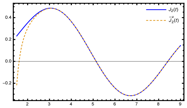
Formula (7), in the domain $t>0$, has discontinuity points at $t={\displaystyle \frac{19}{2\sqrt{246}}}$ and $t={\displaystyle \frac{\sqrt{5}}{2}}$, so we considered it only for $t\ge 4$ to satisfy a more accurate representation (see Figure 1).

Secondly, we consider deducing the new analytic approximation formula:

$${\tilde{J}}_2^v\left(t\right)={\displaystyle \frac{t^8{\cot }^6(t/4)}{r_0+r_1{t}^2+r_2{t}^4+r_3{t}^6+r_4{t}^8}},t>0,$$

where the parameters $r_0,r_1,r_2,r_3,r_4\in R$. Using the general series (1), we have

$$J_2\left(t\right)={\displaystyle \frac{t^2}{8}}-{\displaystyle \frac{t^4}{96}}+{\displaystyle \frac{t^6}{3072}}-{\displaystyle \frac{t^8}{184320}}+{\displaystyle \frac{t^{10}}{17694720}}-{\displaystyle \frac{t^{12}}{2477260800}}+o\left(t^{14}\right),t\to 0.$$

(8)

Also,

$${\cot }^6(t/4)={\displaystyle \frac{4096}{t^6}}+{\displaystyle \frac{t^4}{62370}}-{\displaystyle \frac{512}{t^4}}+{\displaystyle \frac{19t^2}{4725}}+{\displaystyle \frac{368}{15t^2}}-{\displaystyle \frac{502}{945}}+o\left(t^6\right),t\to 0.$$

(9)

Hence, we have

$$\begin{array}{ccc}& & {\displaystyle \frac{1}{8}}{r}_0{t}^2+\left({\displaystyle \frac{r_1}{8}}-{\displaystyle \frac{r_0}{96}}\right)t^4+{\displaystyle \frac{(r_0-32r_1+384r_2)t^6}{3072}}+{\displaystyle \frac{(-r_0+60r_1-1920r_2+23040r_3)t^8}{184320}}\hfill \\ & & +{\displaystyle \frac{(r_0-96r_1+5760r_2-184320r_3+2211840r_4)t^{10}}{17694720}}\hfill \\ & & \sim 4096t^2-512t^4+{\displaystyle \frac{368t^6}{15}}-{\displaystyle \frac{502t^8}{945}}+{\displaystyle \frac{19t^{10}}{4725}},t\to 0.\hfill \end{array}$$

Then we get the following linear system:

$$\begin{array}{ccc}\hfill {\displaystyle \frac{r_0}{8}}-4096& & =0\hfill \\ \hfill -{\displaystyle \frac{r_0}{96}}+{\displaystyle \frac{r_1}{8}}+512& & =0\hfill \\ \hfill {\displaystyle \frac{r_0}{3072}}-{\displaystyle \frac{r_1}{96}}+{\displaystyle \frac{r_2}{8}}-{\displaystyle \frac{368}{15}}& & =0\hfill \\ \hfill -{\displaystyle \frac{r_0}{184320}}+{\displaystyle \frac{r_1}{3072}}-{\displaystyle \frac{r_2}{96}}+{\displaystyle \frac{r_3}{8}}+{\displaystyle \frac{502}{945}}& & =0\hfill \\ \hfill {\displaystyle \frac{r_0}{17694720}}-{\displaystyle \frac{r_1}{184320}}+{\displaystyle \frac{r_2}{3072}}-{\displaystyle \frac{r_3}{96}}+{\displaystyle \frac{r_4}{8}}-{\displaystyle \frac{19}{4725}}& & =0\hfill \end{array}$$

and its unique solution is

$$r_0=32768,r_1=-4096/3,r_2=-128/45,r_3=464/945,r_4=13/2025.$$

Then

$${\tilde{J}}_2^v\left(t\right)={\displaystyle \frac{14175t^8{\cot }^6(t/4)}{91t^8+6960t^6-40320t^4-19353600t^2+464486400}},0<t<4$$

(10)

and

$${\tilde{J}}_2^v\left(0\right)=\underset{t\to 0^{+}}{\lim }{\tilde{J}}_2^v\left(t\right)=0.$$

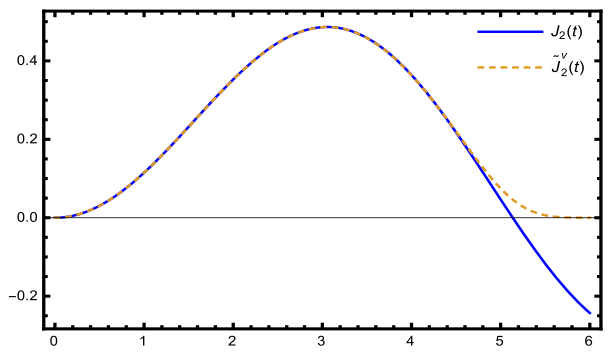
Formula (10), in the domain $t>0$, has no discontinuity points, but we considered it only for $0\le t<4$ to satisfy a more accurate representation (see Figure 2).

At the point $t=4$, the two approximations ${\tilde{J}}_2^u\left(t\right)$ and ${\tilde{J}}_2^v\left(t\right)$ do not coincide. In particular,

$${\tilde{J}}_2^u\left(4\right)=0.364189\dots and{\tilde{J}}_2^v\left(4\right)=0.363737\dots ..$$

3. Results

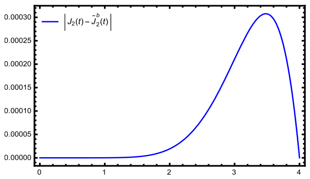
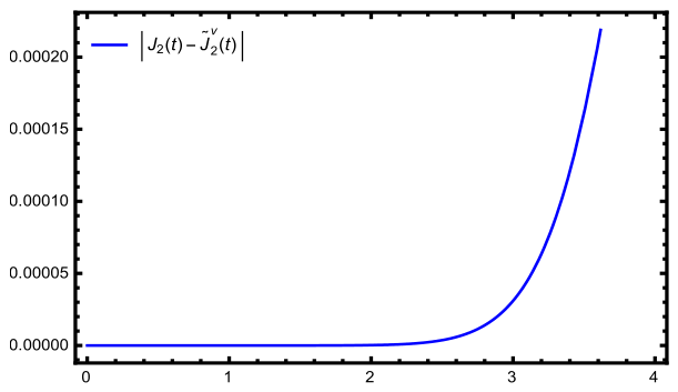
Plotting the absolute errors ${\epsilon }_b\left(t\right)=|J_2\left(t\right)-{\tilde{J}}_2^b\left(t\right)|$ and ${\epsilon }_v\left(t\right)=|J_2\left(t\right)-{\tilde{J}}_2^v\left(t\right)|$ in the interval $0\le t<4$ reveals that the approximation ${\tilde{J}}_2^v\left(t\right)$ is superior to ${\tilde{J}}_2^b\left(t\right)$, where $\max \left({\epsilon }_b\left(t\right)\right)\approx 3\times {10}^{-4}$ and $\max \left({\epsilon }_v\left(t\right)\right)\approx 2\times {10}^{-4}$ (see Figure 3 and Figure 4).

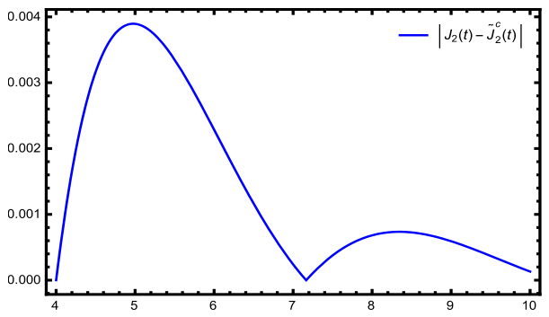
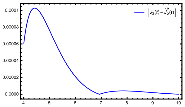
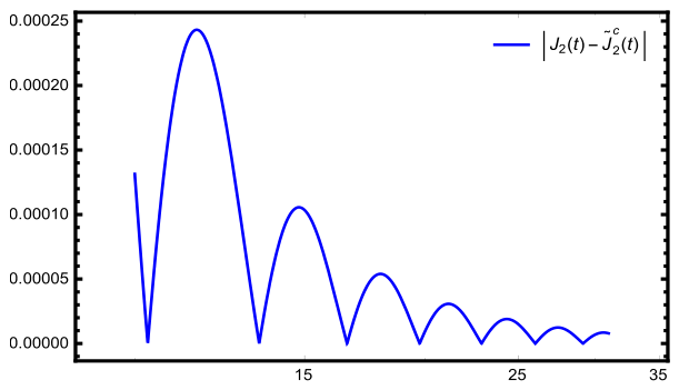
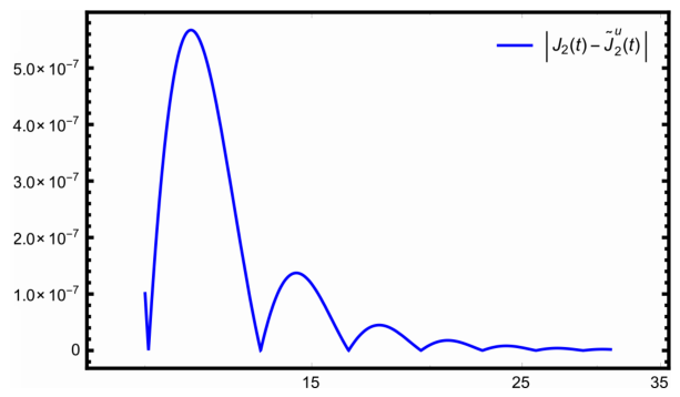
Plotting the absolute errors ${\epsilon }_c\left(t\right)=|J_2\left(t\right)-{\tilde{J}}_2^c\left(t\right)|$ and ${\epsilon }_u\left(t\right)=|J_2\left(t\right)-{\tilde{J}}_2^u\left(t\right)|$ in the interval $t\ge 4$, reveals that the approximation ${\tilde{J}}_2^u\left(t\right)$ is superior to ${\tilde{J}}_2^c\left(t\right)$ (see Figure 5, Figure 6, Figure 7 and Figure 8) since

$$\max \left({\epsilon }_c\left(t\right)\right)\approx 4\times {10}^{-3},\max \left({\epsilon }_u\left(t\right)\right)\approx 1\times {10}^{-4},4\le t\le 10$$

and

$$\max \left({\epsilon }_c\left(t\right)\right)\approx 25\times {10}^{-5},\max \left({\epsilon }_a\left(t\right)\right)\approx 5\times {10}^{-7},10\le t\le 31.$$

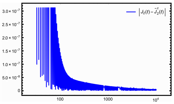
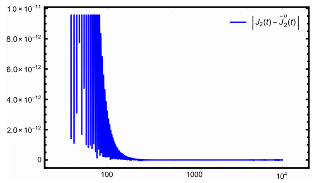
Additionally, Figure 9 and Figure 10 demonstrate how, for large values of the variable t, the approximation ${\tilde{J}}_2^u\left(t\right)$ is superior to the approximation ${\tilde{J}}_2^c\left(t\right)$.

4. Estimating Some Positive Zeros

The positive zeros of the Bessel function $J_2\left(t\right)$ are of fundamental importance in many applications. Therefore, an accurate estimation of these zeros provides an additional measure of the quality of an analytic approximation. In this section, we compute the first twelve positive zeros of the functions $J_2\left(t\right)$, the approximation ${\tilde{J}}_2^c\left(t\right)$, and the proposed approximation ${\tilde{J}}_2^u\left(t\right)$. The computed zeros are listed in

Table 1. The first twelve positive zeros of $J_2\left(t\right)$, ${\tilde{J}}_2^c\left(t\right)$, and ${\tilde{J}}_2^u\left(t\right)$.

n	Zero of ${\mathit{J}}_2\left(\mathit{t}\right)$	Zero of ${\tilde{\mathit{J}}}_2^{\mathit{c}}\left(\mathit{t}\right)$	Zero of ${\tilde{\mathit{J}}}_2^{\mathit{u}}\left(\mathit{t}\right)$
1	5.135622302	5.146898817	5.135819301
2	8.417244140	8.419946058	8.417256488
3	11.619841170	11.620887300	11.619843370
4	14.795951780	14.796463150	14.795952410
5	17.959819490	17.960106990	17.959819720
6	21.116997050	21.117174570	21.116997150
7	24.270112310	24.270229550	24.270112360
8	27.420573550	27.420655010	27.420573580
9	30.569204500	30.569263380	30.569204510
10	33.716519510	33.716563460	33.716519520
11	36.862856510	36.862890180	36.862856520
12	40.008446730	40.008473100	40.008446740

, which provides a direct comparison between the exact zeros and those obtained from the two analytic approximation formulas.

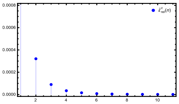
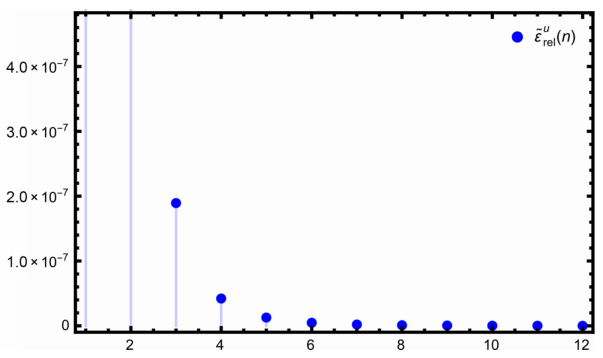
Consider the relative errors ${\tilde{\epsilon }}_{rel}^c\left(n\right)$ and ${\tilde{\epsilon }}_{rel}^u\left(n\right)$ defined by

$${\tilde{\epsilon }}_{rel}^c\left(n\right)={\displaystyle \frac{|t_i-{\tilde{t}}_i^c|}{t_i}}\mathrm{and}{\tilde{\epsilon }}_{rel}^u\left(n\right)={\displaystyle \frac{|t_i-{\tilde{t}}_i^u|}{t_i}},i=1,2,\dots ,12$$

where $t_i$, ${\tilde{t}}_i^c$, and ${\tilde{t}}_i^u$ are the first twelve positive zeros of the functions $J_2\left(t\right)$, ${\tilde{J}}_2^c\left(t\right)$, and ${\tilde{J}}_2^u\left(t\right)$, respectively. The approximation formula ${\tilde{J}}_2^u\left(t\right)$ outperforms ${\tilde{J}}_2^c\left(t\right)$ in estimating positive zeros of the function $J_2\left(t\right)$ for the first twelve ones, as seen in Figure 11 and Figure 12.

The increasing accuracy of the proposed approximation for the higher positive zeros can be explained by the well-known asymptotic distribution of the positive zeros of Bessel functions. In particular, for large n, the nth positive zero of $J_2\left(t\right)$ satisfies $j_{2,n}\sim (n+{\displaystyle \frac{3}{4}})\pi$. Hence, as n increases, the corresponding zeros occur at increasingly large values of t, where the large-argument asymptotic behavior of $J_2\left(t\right)$ becomes increasingly accurate. Since the proposed approximation ${\widehat{J}}_2\left(t\right)$ is constructed to reproduce this asymptotic behavior, its relative agreement with $J_2\left(t\right)$ improves in the large-t region. Consequently, the increasingly accurate approximation of the higher positive zeros observed in Table 1 and Figure 11 and Figure 12 is theoretically consistent with the asymptotic structure of the Bessel function.

5. Conclusions

Using both the asymptotic series as t tends to infinity and the power series of the Bessel function $J_2\left(t\right)$, we get the following new approximation formula:

$${\widehat{J}}_2\left(t\right)=\left\{\begin{array}{cc}{\tilde{J}}_2^u\left(t\right),\hfill & t\ge 4,\hfill \\ {\tilde{J}}_2^v\left(t\right),\hfill & 0\le t<4.\hfill \end{array}\right.$$

(11)

This approximation has a discontinuity at $t=4$ and is more accurate than the analytic approximation formula ${\tilde{J}}_2\left(t\right)$. Also, ${\widehat{J}}_2\left(t\right)$ presents some improvements for estimating the zeros of the Bessel function $J_2\left(t\right)$ better than ${\tilde{J}}_2\left(t\right)$. In the intervals $0\le t<4$, $4\le t\le 10$, and $10\le x<31$, respectively, the approximate numerically observed maximum absolute errors between $J_2\left(t\right)$ and ${\widehat{J}}_2\left(t\right)$ achieved here are $0.0002$, $0.0001$, and $4\times {10}^{-7}$ (see Figure 4, Figure 6 and Figure 8). Additionally, our new approximation’s absolute error will decrease significantly as t increases, and it has a superiority over the approximation’s absolute error ${\tilde{J}}_2\left(t\right)$ in the domain $31\le t\le {10}^4$ (see Figure 9 and Figure 10). Our analysis of the absolute error between $J_2\left(t\right)$ and ${\widehat{J}}_2\left(t\right)$ in the interval $[0,{10}^4]$ shows it decreases significantly as t increases for large t. Furthermore, our new approximation formula ${\widehat{J}}_2\left(t\right)$ presents estimations of the first twelve positive zeros of the function $J_2\left(t\right)$ more accurately than the approximation formula ${\tilde{J}}_2\left(t\right)$, and with increasing t, the zeros of $J_2\left(t\right)$ and ${\widehat{J}}_2\left(t\right)$ are very close (see Figure 12). With the appropriate adjustments to account for the characteristics and nature of each function, the methodology used in this study can theoretically be extended to some types of oscillatory special functions. The present work demonstrates that simple analytic approximations expressed in terms of elementary functions can achieve a high level of accuracy while remaining computationally efficient. Compared with previously published approximations, the proposed formula provides a better balance between simplicity and accuracy by improving the approximation of both the function values and its positive zeros over a wide interval. Consequently, the proposed approximation offers a practical alternative for applications requiring repeated evaluations of the Bessel function $J_2\left(t\right)$, such as numerical simulations, engineering computations, and iterative algorithms, where computational efficiency is essential. Moreover, the approximation strategy developed in this paper provides a general framework that may be adapted to construct accurate elementary approximations for other oscillatory special functions.

References

1. Arfken, G.B.; Weber, H.J.; Harris, F.E. Mathematical Methods for Physicists, 7th ed.; Academic Press, Elsevier: San Diego, CA, USA, 2013. [Google Scholar]
2. Abramowitz, M.; Stegun, I.A. Handbook of Mathematical Functions with Formulas, Graphs, and Mathematical Tables; Dover Publications: New York, NY, USA, 1964. [Google Scholar]
3. National Institute of Standards and Technology. Digital Library of Mathematical Functions (DLMF); U.S. Department of Commerce: Gaithersburg, MD, USA, 2016.
4. Watson, G.N. A Treatise on the Theory of Bessel Functions; Cambridge University Press: Cambridge, UK, 1922. [Google Scholar]
5. Nemes, G. Error Bounds for the Large-Argument Asymptotic Expansions of the Hankel and Bessel Functions. Acta Appl. Math. 2017, 150, 141–177. [Google Scholar] [CrossRef] [Scilit]
6. Olver, F.W.J. Asymptotics and Special Functions; AK Peters/CRC Press: Wellesley, MA, USA, 1974. [Google Scholar]
7. Baratella, P.; Garetto, M.; Vinardi, G. Approximation of the Bessel Function Jν(x) by Numerical Integration. J. Comput. Appl. Math. 1981, 7, 87–91. [Google Scholar] [CrossRef] [Scilit]
8. Guerrero, A.L.; Martin, P. Higher Order Two-Point Quasi-Fractional Approximations to the Bessel Functions J0(x) and J1(x). J. Comput. Phys. 1988, 77, 276–281. [Google Scholar] [CrossRef] [Scilit]
9. Maass, F.; Martin, P.; Olivares, J. Analytic Approximation to the Bessel Function J0(x). Comput. Appl. Math. 2020, 39, 222. [Google Scholar] [CrossRef] [Scilit]
10. Molinari, L.G. A Note on Trigonometric Approximations of Bessel Functions of the First Kind, and Trigonometric Power Sums. Fundam. J. Math. Appl. 2022, 5, 266–272. [Google Scholar] [CrossRef] [Scilit]
11. Maass, F.; Martin, P. Precise Analytic Approximations for the Bessel Function J1(x). Results Phys. 2018, 8, 1234–1238. [Google Scholar] [CrossRef] [Scilit]
12. Maass, F.; Martin, P. A New Method to Obtain Analytic Approximations Applied to the J1(x) Function. J. Phys. Conf. Ser. 2018, 1043, 012002. [Google Scholar] [CrossRef] [Scilit]
13. Millane, R.P.; Eads, J.L. Polynomial Approximations to Bessel Functions. IEEE Trans. Antennas Propag. 2003, 51, 1398–1400. [Google Scholar] [CrossRef]
14. Harrison, J. Fast and Accurate Bessel Function Computation. In Proceedings of the 2009 19th IEEE Symposium on Computer Arithmetic, Portland, OR, USA, 8–10 June 2009; IEEE: New York, NY, USA, 2009; pp. 104–113. [Google Scholar]
15. Yang, Z.H.; Chu, Y.M. On Approximating the Modified Bessel Function of the First Kind and Toader-Qi Mean. J. Inequal. Appl. 2016, 2016, 40. [Google Scholar] [CrossRef] [Scilit]
16. Yang, Z.H.; Chu, Y.M. On Approximating the Modified Bessel Function of the Second Kind. J. Inequal. Appl. 2017, 2017, 41. [Google Scholar] [CrossRef] [Scilit] [PubMed]
17. Cuyt, A.; Lee, W.; Wu, M. High Accuracy Trigonometric Approximations of the Real Bessel Functions of the First Kind. Comput. Math. Math. Phys. 2020, 60, 119–127. [Google Scholar] [CrossRef] [Scilit]
18. Funes, J.O.; Kari, E.R.V.; Martin, P. The Modified Bessel Functions I3/4(x) and I-3/4(x) in Certain Fractional Differential Equations. J. Phys. Conf. Ser. 2021, 1730, 012065. [Google Scholar] [CrossRef] [Scilit]
19. Martin, P.; Rojas, E.; Olivares, J.; Sotomayor, A. Quasi-Rational Analytic Approximation for the Modified Bessel Function I1(x) with High Accuracy. Symmetry 2021, 13, 741. [Google Scholar] [CrossRef] [Scilit]
20. Blachman, N.M.; Mousavinezhad, S.H. Trigonometric approximations for Bessel functions. IEEE Trans. Aerosp. Electron. Syst. 1986, AES-22, 2–7. [Google Scholar] [CrossRef]
21. Li, L.-L.; Li, F.; Gross, F.B. A new polynomial approximation for Jν Bessel functions. Appl. Math. Comput. 2006, 183, 1220–1225. [Google Scholar] [CrossRef] [Scilit]
22. Krasikov, I. Approximations for the Bessel and Airy functions with an explicit error term. Lms J. Comput. Math. 2014, 17, 209–225. [Google Scholar] [CrossRef] [Scilit]
23. Čağlar, M.; Deniz, E.; Kazımoğlu, S. Neighborhoods of Certain Classes of Analytic Functions Defined by Normalized Function az2 J ϑ (z) + bz J ϑ (z) + c J ϑ (z). Turk. J. Sci. 2020, 5, 226–232. [Google Scholar] [CrossRef] [Scilit]
24. Toklu, E.; Kara, O. Radii Problems for Normalized Hyper-Bessel Function. Turk. J. Sci. 2020, 5, 16–22. [Google Scholar] [CrossRef] [Scilit]
25. Martin, P.; Ramos-Andrade, J.P.; Caro-Pérez, F.; Lastra, F. Accurate Analytical Approximation for the Bessel Function J2(x). Math. Comput. Appl. 2024, 29, 63. [Google Scholar] [CrossRef] [Scilit]
26. Mahmoud, M.; Almuashi, H. An Improved Analytical Approximation of the Bessel Function J2(x). Axioms 2025, 14, 157. [Google Scholar] [CrossRef] [Scilit]
Figure 1. The graphs of J 2 ( t ) and J ˜ 2 u ( t ) for 1.5 t 9 . The figure shows that the approximation J ˜ 2 u ( t ) closely follows the Bessel function J 2 ( t ) over t 4 .
Symmetry 18 01486 g001
Figure 2. The graphs of J 2 ( t ) and J ˜ 2 v ( t ) for 0 t 6 . The close agreement between the two graphs demonstrates the accuracy of J ˜ 2 v ( t ) on 0 t < 4 .
Symmetry 18 01486 g002
Figure 3. The absolute error ε b ( t ) = | J 2 ( t ) J ˜ 2 b ( t ) | for 0 t < 4 .
Symmetry 18 01486 g003
Figure 4. The absolute error ε v ( t ) = | J 2 ( t ) J ˜ 2 v ( t ) | for 0 t < 4 . The figure demonstrates that J ˜ 2 v ( t ) provides an accurate approximation to J 2 ( t ) in this interval.
Symmetry 18 01486 g004
Figure 5. The absolute error ε c ( t ) = | J 2 ( t ) J ˜ 2 c ( t ) | .
Symmetry 18 01486 g005
Figure 6. The absolute error ε u ( t ) = | J 2 ( t ) J ˜ 2 u ( t ) | for 4 t < 10 . The figure demonstrates that J ˜ 2 u ( t ) provides an accurate approximation to J 2 ( t ) in this interval.
Symmetry 18 01486 g006
Figure 7. The absolute error ε c ( t ) = | J 2 ( t ) J ˜ 2 c ( t ) | for 10 t < 31 .
Symmetry 18 01486 g007
Figure 8. The absolute error ε u ( t ) = | J 2 ( t ) J ˜ 2 u ( t ) | for 10 t < 31 . The figure demonstrates that J ˜ 2 u ( t ) provides an accurate approximation to J 2 ( t ) in this interval.
Symmetry 18 01486 g008
Figure 9. The absolute error ε c ( t ) = | J 2 ( t ) J ˜ 2 c ( t ) | for 31 t < 10 4 , shown on a logarithmic vertical scale.
Symmetry 18 01486 g009
Figure 10. The absolute error ε u ( t ) = | J 2 ( t ) J ˜ 2 u ( t ) | for 31 t < 10 4 , shown on a logarithmic vertical scale. The figure demonstrates the accuracy of J ˜ 2 u ( t ) as an approximation to J 2 ( t ) on this interval.
Symmetry 18 01486 g010
Figure 11. The relative error between the zeros of J 2 ( t ) and J ˜ 2 c ( t ) , ε ˜ r e l c ( n ) = | t i t ˜ i c | t i for i = 1 , 2 , , 12 .
Symmetry 18 01486 g011
Figure 12. The relative error between the zeros of J 2 ( t ) and J ˜ 2 u ( t ) , ε ˜ rel u ( n ) = | t i t ˜ i u | t i , i = 1 , 2 , , 12 . The relative error remains very small, indicating that J ˜ 2 u ( t ) provides accurate approximations of the first twelve positive zeros of J 2 ( t ) .
Symmetry 18 01486 g012