Recent Advances in Stability for Inverse Inclusion Problems in Electrical Impedance Tomography

Abstract

Inverse inclusion problems arise in several applications such as electrical impedance tomography, nondestructive testing, and geophysical imaging. The purpose of this review is to present some recent advances concerning stability estimates for the determination of inclusions from boundary measurements. We focus on elliptic conductivity equations with discontinuous coefficients and discuss different settings including isotropic and anisotropic conductivities, variable coefficients, local boundary measurements, and layered media. Particular attention is devoted to the analytical tools underlying logarithmic stability estimates, namely singular solutions, asymptotic analysis of fundamental solutions, quantitative unique continuation, and propagation of smallness arguments. We also compare different stability regimes, emphasizing how finite-dimensional geometric priors, such as polygonal or polyhedral inclusions, may lead to Hölder or Lipschitz stability estimates in contrast with the logarithmic stability typical of broader infinite-dimensional classes. We highlight how a common methodological framework can be adapted to increasingly complex geometrical and physical configurations. Finally, we briefly discuss some open problems and possible future developments in the study of inverse inclusion problems.

1. Introduction

Inverse boundary value problems arise naturally in several areas of applied mathematics and mathematical physics, including electrical impedance tomography, nondestructive testing, medical imaging, and geophysical prospection. Among them, inverse inclusion problems constitute an important class of problems in which the objective is to determine an unknown inclusion embedded in a conducting medium by means of measurements performed on the boundary of the domain.

A classical framework is provided by the inverse conductivity problem introduced by Calderón [1]. Let $\mathsf{\Omega }\subset {\mathbb{R}}^n$, $n\ge 2$, be a bounded domain representing an electrical conductor and let $D\subset \mathsf{\Omega }$ denote an unknown inclusion. In many physical situations, the inclusion corresponds to an anomalous region whose conductivity differs from that of the surrounding background medium. The conductivity coefficient is therefore modeled by a discontinuous function across the interface $\partial D$. A typical example is

$$\gamma \left(x\right)=a\left(x\right)+(b\left(x\right)-a\left(x\right)){\chi }_D\left(x\right),$$

where $a\left(x\right)$ denotes the background conductivity, $b\left(x\right)$ is the conductivity inside the inclusion, and ${\chi }_D$ is the characteristic function of the set D.

Prescribing a voltage potential f on the boundary $\partial \mathsf{\Omega }$, the induced electric potential u satisfies the elliptic equation

$$\mathrm{div}\left(\gamma \right(x)\nabla u)=0\mathrm{in}\mathsf{\Omega }.$$

The corresponding current density measured on the boundary defines the so-called Dirichlet-to-Neumann map, which represents the available boundary measurements. The inverse inclusion problem involves determining information about the unknown set D from the knowledge of this operator.

The unique determination of inclusions from boundary measurements has been extensively investigated starting from the pioneering work of Isakov [2]. However, uniqueness alone is not sufficient for applications. In practical measurements, one always deals with noisy data and therefore a fundamental issue concerns stability estimates, namely the quantitative dependence of the unknown inclusion on the measured data. More precisely, given two admissible inclusions $D_1$ and $D_2$, one seeks estimates of the form

$$d_H(\partial D_1,\partial D_2)\le \omega \left(\parallel {\mathsf{\Lambda }}_{D_1}-{\mathsf{\Lambda }}_{D_2}\parallel \right),$$

where $d_H$ denotes the Hausdorff distance and $\omega$ is a modulus of continuity.

The stability properties of inverse inclusion problems depend strongly on the class of admissible geometries and on the amount of a priori information available. For broad infinite-dimensional classes of inclusions with smooth boundaries, logarithmic stability is the typical regime. Exponential instability results for specific admissible classes show that such logarithmic-type estimates are, in those settings, essentially optimal [3]. For the admissible classes of $C^{1,\alpha }$ inclusions considered in [4], estimates of the form

$$d_H(\partial D_1,\partial D_2)\le C{\left|\log \epsilon \right|}^{-\eta },$$

where $\epsilon = \parallel {\mathsf{\Lambda }}_{D_1}-{\mathsf{\Lambda }}_{D_2}\parallel ,$ and $C>0$, $\eta \in (0,1)$ depend only on the a priori data, have been established in the isotropic piecewise constant setting [4]. This logarithmic regime should not, however, be interpreted as a universal threshold for inverse inclusion problems. Stronger stability estimates may be obtained when additional structural information reduces the admissible set of inclusions to a finite-dimensional geometric class. Depending on the geometry and on the measurement setting, Hölder or even Lipschitz stability may then become available. The distinction between these different stability regimes is one of the themes considered below and will be discussed in detail in Section 4.

Starting from the first stability results for piecewise constant isotropic conductivities, the analysis has progressively evolved toward more sophisticated physical and geometrical settings. Stability estimates have been obtained for variable coefficient conductivities [5], local boundary measurements [5], anisotropic media [6], and layered conductors with transmission interfaces [7,8]. Although the complexity of the analysis increases substantially in these frameworks, a common methodological structure emerges rather clearly.

A complementary line of research has investigated stability under finite-dimensional geometric priors. In particular, results for polygonal and polyhedral conductivity inclusions have established Lipschitz stability from full or local boundary measurements [9,10,11], while improved stability has also been obtained under strongly reduced measurement configurations [12,13].

More recent developments have increasingly focused on the interaction between finite-dimensional geometric information and reduced boundary data. Alberti, Arroyo and Santacesaria obtained Lipschitz stability from finitely many measurements for a conductivity with an unknown triangular inclusion within a general framework for inverse problems on low-dimensional manifolds [14]. Hanke subsequently proved Lipschitz stability for a planar polygonal conductivity inclusion from only two suitable Cauchy data pairs; in the insulating case, a single Cauchy pair is sufficient [15]. Recent work has also addressed the simultaneous determination of polygonal geometry and an unknown constant conductivity value [16], while a recent three-dimensional result establishes logarithmic stability for convex polyhedral inclusions from a single boundary measurement [17]. The latter two contributions are currently available as preprints.

Taken together, these developments show a clear recent trend toward quantitative stability with progressively reduced measurement sets and toward the simultaneous recovery of geometric and conductivity parameters. These developments will be discussed in Section 4.

The purpose of this review is to present some recent advances concerning stability estimates for inverse inclusion problems associated with elliptic conductivity equations, focusing on the analytical mechanisms underlying the stability results and on the evolution of a unified strategy capable of treating increasingly complex conductivity models.

The core of the analysis relies on the interaction between two main ingredients. The first one is the use of singular solutions and asymptotic estimates for the associated fundamental solutions near the inclusion boundary. The second one is quantitative unique continuation, achieved through tools such as three-spheres inequalitiy, propagation of smallness arguments, and Carleman estimates [18,19,20]. Roughly speaking, the discrepancy of the boundary measurements is propagated from the boundary of the domain toward the unknown inclusion, while singular solutions amplify the sensitivity of the estimates near the interface. The combination of these two mechanisms eventually leads to logarithmic stability estimates in terms of the Hausdorff distance between inclusions.

A remarkable aspect of this approach is its robustness. Although anisotropic conductivities, discontinuous backgrounds, and layered media introduce substantial technical difficulties, the same general scheme can still be adapted successfully. In particular, the asymptotic analysis of singular solutions near interfaces and transmission boundaries plays a crucial role throughout the theory.

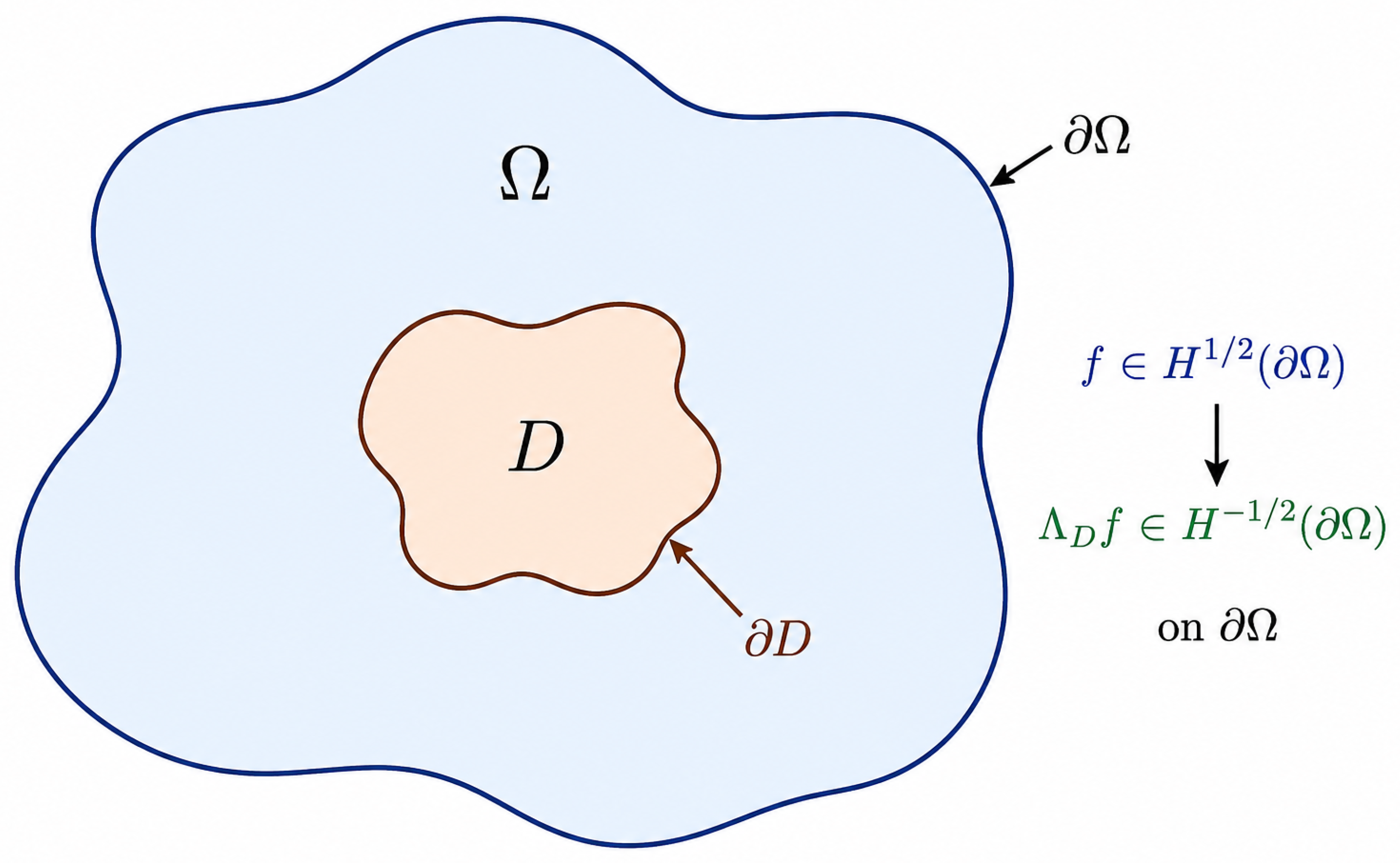
A schematic configuration of the inverse inclusion problem is illustrated in Figure 1.

The paper is organized as follows: In Section 2, we introduce the mathematical framework and the notion of stability for inverse inclusion problems. Section 3 is devoted to the main analytical tools underlying the derivation of logarithmic stability estimates, including Alessandrini type identities, singular solutions, and quantitative unique continuation arguments. In Section 4, we discuss stability results for different conductivity models, with particular attention to anisotropic conductivities and layered media. Finally, in Section 5, we address some open problems and possible future developments.

2. Mathematical Framework

In this section, we introduce the mathematical setting of inverse inclusion problems and the notion of stability that will be considered throughout the paper. We mainly focus on elliptic conductivity equations with discontinuous coefficients, although many of the ideas discussed below extend to more general inverse boundary value problems.

Let $\mathsf{\Omega }\subset {\mathbb{R}}^n$, $n\ge 2$, be a bounded Lipschitz domain and let $D⋐\mathsf{\Omega }$ denote an unknown inclusion. We assume that the conductivity coefficient presents a jump discontinuity across the interface $\partial D$. A typical model is given by

$${\gamma }_D\left(x\right)=a\left(x\right)+(b\left(x\right)-a\left(x\right)){\chi }_D\left(x\right),$$

(1)

where ${\chi }_D$ denotes the characteristic function of the set D, the function $a\left(x\right)$ represents the known background conductivity, and $b\left(x\right)$ describes the conductivity inside the inclusion.

Given a boundary datum $f\in H^{1/2}(\partial \mathsf{\Omega })$, the corresponding electric potential $u\in H^1\left(\mathsf{\Omega }\right)$ is the weak solution of the Dirichlet problem

$$\left\{\begin{array}{cc}\hfill \mathrm{div}\left(\gamma \right(x)\nabla u)& =0\mathrm{in}\mathsf{\Omega },\hfill \\ \hfill u& =f\mathrm{on}\partial \mathsf{\Omega }.\hfill \end{array}\right.$$

(2)

The associated Dirichlet-to-Neumann map is the bounded operator

$${\mathsf{\Lambda }}_D:H^{1/2}(\partial \mathsf{\Omega })⟶H^{-1/2}(\partial \mathsf{\Omega }),$$

(3)

defined in the weak sense through the duality relation

$$〈{\mathsf{\Lambda }}_{D}f,g〉={\int }_{\mathsf{\Omega }}{\gamma }_D\left(x\right)\nabla u_f\left(x\right)·\nabla v_g\left(x\right)dx,$$

(4)

for every $f,g\in H^{1/2}(\partial \mathsf{\Omega })$, where $u_f\in H^1\left(\mathsf{\Omega }\right)$ is the weak solution of the conductivity equation with boundary datum f, and $v_g\in H^1\left(\mathsf{\Omega }\right)$ is any function whose trace on $\partial \mathsf{\Omega }$ is g. The right-hand side of Equation (4) is independent of the choice of the extension $v_g$.

For sufficiently regular solutions, this weak definition agrees with the classical conormal derivative

$${\mathsf{\Lambda }}_{D}f={\gamma }_D\nabla u_f·\nu ={\gamma }_D{\displaystyle \frac{\partial u_f}{\partial \nu }}{|}_{\partial \mathsf{\Omega }},$$

where $\nu$ denotes the outward unit normal vector to $\partial \mathsf{\Omega }$. Physically, the Dirichlet-to-Neumann map associates an applied boundary voltage with the corresponding boundary current density. Throughout the paper, when the conductivity is parametrized by an inclusion D, we write ${\mathsf{\Lambda }}_D$ for the corresponding Dirichlet-to-Neumann map. When two general conductivity coefficients ${\gamma }_1$ and ${\gamma }_2$ are compared independently of an inclusion parametrization, we use the notation ${\mathsf{\Lambda }}_{{\gamma }_1}$ and ${\mathsf{\Lambda }}_{{\gamma }_2}$.

The inverse inclusion problem involves determining the unknown set D from the knowledge of the map ${\mathsf{\Lambda }}_D$. More generally, one may also consider local boundary measurements, partial Dirichlet-to-Neumann maps, or Neumann-to-Dirichlet maps. Similar questions arise as well in anisotropic media and in layered conductors.

A Priori Assumptions

Since inverse inclusion problems are severely ill-posed, stability estimates can only be expected under suitable a priori assumptions on the geometry and regularity of the unknown inclusion.

Typically, one assumes the following:

(i)

The domain $\mathsf{\Omega }$ has boundary of class $C^{1,\alpha }$;

(ii)

The inclusion D has boundary of class $C^{1,\alpha }$;

(iii)

The inclusion stays at positive distance from the exterior boundary, that is

$$\mathrm{dist}(D,\partial \mathsf{\Omega })\ge \delta >0;$$

(iv)

The background region $\mathsf{\Omega }\setminus D$ is connected.

Such assumptions play an essential role both in the asymptotic analysis of singular solutions and in the application of quantitative unique continuation arguments.

The regularity of the interface $\partial D$ is particularly important in order to flatten the boundary locally and compare the conductivity equation with suitable model transmission problems. Moreover, the connectedness of the background region is required in the propagation of smallness arguments, which rely on chains of balls connecting the boundary measurements to the unknown inclusion.

The precise a priori assumptions depend on the conductivity model under consideration. In order to state a representative stability result, we first consider the basic isotropic piecewise constant model

$${\gamma }_D\left(x\right)=1+(k-1){\chi }_D\left(x\right),$$

(5)

where the background conductivity is known and normalized to 1, and $k>0$, $k\ne 1$, is a fixed and known conductivity contrast. Thus, the conductivity is uniformly elliptic and the jump across $\partial D$ is nonvanishing.

Stability Estimates

A central issue concerns the quantitative stability of the inverse problem. Let $D_1$ and $D_2$ be two admissible inclusions and let ${\mathsf{\Lambda }}_{D_1}$ and ${\mathsf{\Lambda }}_{D_2}$ denote the corresponding Dirichlet-to-Neumann maps. One seeks estimates of the form

$$d_H(\partial D_1,\partial D_2)\le \omega \left(\parallel {\mathsf{\Lambda }}_{D_1}-{\mathsf{\Lambda }}_{D_2}\parallel \right),$$

(6)

where $d_H$ denotes the Hausdorff distance between sets and $\omega$ is a modulus of continuity.

Theorem 1 (Representative logarithmic stability estimate).

Let $\mathsf{\Omega }\subset {\mathbb{R}}^n$, $n\ge 2$, be a bounded domain such that

$$\left|\mathsf{\Omega }\right|\le M{r}^n$$

and $\partial \mathsf{\Omega }$ is of class $C^{1,\alpha }$ with uniform constants $r,L>0$. Let $D_1,D_2⋐\mathsf{\Omega }$ satisfy

$$\mathrm{dist}(D_i,\partial \mathsf{\Omega })\ge \delta >0,\mathsf{\Omega }\setminus \overline{D_i}\mathit{is}\mathit{connected},i=1,2,$$

and assume that $\partial D_i$ is of class $C^{1,\alpha }$ with the same uniform constants $r,L$.

Consider

$${\gamma }_{D_i}\left(x\right)=1+(k-1){\chi }_{D_i}\left(x\right),i=1,2,$$

where $k>0$, $k\ne 1$, is fixed and known. Let ${\mathsf{\Lambda }}_{D_i}$ denote the corresponding Dirichlet-to-Neumann maps. Then, there exists an increasing function $\omega :[0,+\infty )\to [0,+\infty )$ such that

$$d_H(\partial D_1,\partial D_2)\le \omega (\parallel {\mathsf{\Lambda }}_{D_1}-{\mathsf{\Lambda }}_{D_2}{\parallel }_{\mathcal{L}(H^{1/2}(\partial \mathsf{\Omega }),H^{-1/2}(\partial \mathsf{\Omega }))}),$$

and

$$\omega \left(t\right)\le {C\left|\log t\right|}^{-\eta },0<t<1,$$

where $C>0$ and $\eta \in (0,1]$ depend only on the a priori data

$$k,n,r,M,\delta ,L,\alpha .$$

Theorem 1 reproduces, in a slightly streamlined notation, the representative logarithmic stability result for the isotropic piecewise constant model established in [4]. The assumptions and stability regimes associated with variable, anisotropic, layered, and finite-dimensional geometric models are discussed separately in Section 4.

Modified Distance

Besides the Hausdorff distance, it is often convenient to introduce suitable auxiliary notions of distance between inclusions. A particularly useful quantity is the so-called modified distance, which naturally arises in the analysis based on singular solutions (see [21]).

Let $D_1$ and $D_2$ be two admissible inclusions and let G denote the connected component of

$$\mathsf{\Omega }\setminus \overline{(D_1\cup D_2)}$$

whose boundary contains $\partial \mathsf{\Omega }$. Defining

$${\mathsf{\Omega }}_D=\mathsf{\Omega }\setminus G,$$

the modified distance is given by

$$d_{\mu }(D_1,D_2)=\max \left\{\underset{x\in \partial D_1\cap \partial {\mathsf{\Omega }}_D}{\sup }\mathrm{dist}(x,D_2),\underset{x\in \partial D_2\cap \partial {\mathsf{\Omega }}_D}{\sup }\mathrm{dist}(x,D_1)\right\}.$$

(7)

In general, $d_{\mu }$ does not define a metric and does not dominate the Hausdorff distance. Under the geometric assumptions of the representative isotropic setting introduced above, however, the following estimate holds; it corresponds to Proposition 3.3 of [4], expressed in the notation used here.

Proposition 1 (Modified distance and Hausdorff distance).

Under the $C^{1,\alpha }$ regularity, separation, and connectedness assumptions stated above, there exists a constant $C>0$, depending only on the corresponding geometric a priori parameters, such that

$$d_H(\partial D_1,\partial D_2)\le C{d}_{\mu }(D_1,D_2).$$

The introduction of the modified distance is particularly convenient because the singular solution arguments naturally provide estimates on points realizing $d_{\mu }$, which can then be transferred to the Hausdorff distance through Proposition 1.

Different Conductivity Models

Several conductivity models have been considered in the literature.

In the isotropic case, the conductivity coefficient is scalar valued and the inclusion is modeled through a jump discontinuity across $\partial D$. More general situations involve variable coefficient conductivities, where both the background and the inclusion conductivity may depend on the space variable.

Another important framework concerns anisotropic conductivities, where the conductivity is represented by a symmetric positive definite matrix valued function, $\gamma \left(x\right)=A\left(x\right).$ In this case, the geometry induced by the matrix coefficient strongly affects the behavior of the singular solutions and the propagation of quantitative information.

Finally, inverse inclusion problems in layered media involve conductivity coefficients presenting discontinuities across known transmission interfaces. Such configurations are particularly relevant in geophysical applications and lead naturally to transmission problems with discontinuous coefficients.

Although these settings introduce substantial technical difficulties, the corresponding stability analyses share several common analytical features. In the next section, we discuss the main analytical tools underlying the derivation of logarithmic stability estimates for inverse inclusion problems.

3. Analytical Tools for Stability Estimates

In this section, we discuss the main analytical ingredients underlying the derivation of logarithmic stability estimates for inverse inclusion problems. Although the physical settings and the conductivity models may vary considerably, most of the available stability results rely on a common strategy combining integral identities, singular solutions, quantitative unique continuation, and geometric constructions based on chains of balls, tubular neighborhoods, and truncated cones.

At a conceptual level, the mechanism leading to stability estimates may be summarized as follows:

$$\parallel {\mathsf{\Lambda }}_{D_1}-{\mathsf{\Lambda }}_{D_2}\parallel ⟹\mathrm{propagation}\mathrm{of}\mathrm{smallness}⟹\mathrm{control}\mathrm{near}\partial D$$

combined with the singular behavior of suitable fundamental solutions near the inclusion boundary. The interaction between these two mechanisms eventually produces quantitative estimates on the distance between inclusions.

A fundamental role in the analysis is played by Alessandrini’s identity. Let ${\gamma }_1$ and ${\gamma }_2$ be two conductivity coefficients and let $u_i\in H^1\left(\mathsf{\Omega }\right)$, $i=1,2$, be weak solutions of

$$\mathrm{div}({\gamma }_i\nabla u_i)=0\mathrm{in}\mathsf{\Omega },$$

with boundary traces

$$u_i{|}_{\partial \mathsf{\Omega }}=f_i,f_i\in H^{1/2}(\partial \mathsf{\Omega }).$$

Then

$$〈({\mathsf{\Lambda }}_{{\gamma }_1}-{\mathsf{\Lambda }}_{{\gamma }_2})f_1,f_2〉={\int }_{\mathsf{\Omega }}({\gamma }_1-{\gamma }_2)\nabla u_1·\nabla u_{2}dx.$$

(8)

Formula (8) establishes a direct relation between the difference of the boundary measurements and the discrepancy of the conductivity coefficients inside the domain. In particular, it transforms boundary information into interior integral estimates.

The key idea involves choosing suitable singular solutions in Alessandrini’s identity. To illustrate the construction, consider the basic isotropic model

$${\gamma }_{D_i}\left(x\right)=1+(k-1){\chi }_{D_i}\left(x\right),i=1,2,$$

with the same fixed contrast $k>0$, $k\ne 1$. Let ${\mathsf{\Gamma }}_{D_i}(x,y)$ denote the fundamental solution associated with the operator $\mathrm{div}({\gamma }_{D_i}\nabla ·)$. For singularities $y,w$ lying in the connected component of $\mathsf{\Omega }\setminus \overline{(D_1\cup D_2)}$ that communicates with $\partial \mathsf{\Omega }$, one introduces the interaction functional

$$S(y,w)=(k-1){\int }_{\mathsf{\Omega }}({\chi }_{D_1}-{\chi }_{D_2}){\nabla }_x{\mathsf{\Gamma }}_{D_1}(x,y)·{\nabla }_x{\mathsf{\Gamma }}_{D_2}(x,w)dx.$$

(9)

Equivalently,

$$\begin{array}{cc}\hfill S(y,w)=& (k-1){\int }_{D_1\setminus D_2}{\nabla }_x{\mathsf{\Gamma }}_{D_1}(x,y)·{\nabla }_x{\mathsf{\Gamma }}_{D_2}(x,w)dx\hfill \\ \hfill & -(k-1){\int }_{D_2\setminus D_1}{\nabla }_x{\mathsf{\Gamma }}_{D_1}(x,y)·{\nabla }_x{\mathsf{\Gamma }}_{D_2}(x,w)dx.\hfill \end{array}$$

(10)

Thus, $S(y,w)$ measures the interaction of the two singular solutions over the symmetric difference of the inclusions. As y and w approach a suitable point of the inclusion boundary from the exterior region, the singular behavior of the fundamental solutions makes (9) sensitive to the geometric discrepancy between $D_1$ and $D_2$. This provides the lower-bound mechanism that is combined with quantitative propagation of smallness in the stability argument.

One of the major difficulties in inverse inclusion problems comes from the presence of discontinuous coefficients. In order to overcome this issue, singular solutions associated with the conductivity operator are introduced.

Let ${\mathsf{\Gamma }}_D(x,y)$ denote the fundamental solution associated with the operator

$$\mathrm{div}({\gamma }_D\left(x\right)\nabla ·).$$

Classical Green-function theory for uniformly elliptic equations with bounded measurable coefficients provides pointwise bounds for ${\mathsf{\Gamma }}_D$; see Littman–Stampacchia–Weinberger [22]. These estimates should be distinguished from the piecewise gradient regularity available for elliptic equations with discontinuous coefficients. In particular, Theorem 1 of Li and Vogelius [23] provides piecewise $C^{1,{\alpha }_0}$ estimates under piecewise Hölder regularity of the coefficients and $C^{1,\alpha }$ regularity of the interfaces.

For the isotropic piecewise constant conductivity model considered here, the corresponding estimates for the fundamental solution are collected in Proposition 3.4 of [4]. In particular, Proposition 3.4(i) gives

$$|{\nabla }_x{\mathsf{\Gamma }}_D{(x,y)|\le C|x-y|}^{1-n}.$$

(11)

Moreover, Proposition 3.4(ii) provides the more precise interface asymptotics obtained by comparison with the fundamental solution ${\mathsf{\Gamma }}_{+}$ of the flat transmission problem

$$|{\mathsf{\Gamma }}_D(x,y)-{\mathsf{\Gamma }}_{+}{(x,y)|\le C|x-y|}^{2-n+\alpha },$$

(12)

and, in the corresponding local configuration,

$$|{\nabla }_x{\mathsf{\Gamma }}_D(x,y)-{\nabla }_x{\mathsf{\Gamma }}_{+}{(x,y)|\le C|x-y|}^{1-n+{\alpha }^2},$$

(13)

where the constants also contain the appropriate scaling factors associated with the a priori $C^{1,\alpha }$ regularity parameters.

These interface asymptotics are substantially more precise than general Green-function bounds and constitute the local information required in the singular-solution stability argument.

The situation becomes substantially more delicate in anisotropic conductivities or layered media. In these settings, the geometries induced by the matrix coefficient and the transmission conditions across interfaces strongly affect the singular behavior of the solutions.

In the anisotropic framework, explicit expressions for the fundamental solutions are generally unavailable. Consequently, one needs refined comparison arguments with model operators and more sophisticated asymptotic estimates. Similarly, in layered media, the presence of transmission interfaces modifies the local structure of the singularities and requires a careful analysis of the corresponding transmission problem.

Despite these additional difficulties, the overall mechanism remains essentially the same. Lower bounds are obtained from the singular asymptotics near the inclusion boundary, while upper bounds are derived from the discrepancy of the boundary measurements.

The second fundamental ingredient in the derivation of stability estimates is quantitative unique continuation. Roughly speaking, these techniques allow one to propagate the smallness of the discrepancy of the measurements from the boundary of the domain toward the unknown inclusion.

A basic quantitative unique continuation tool is the three-spheres inequality. Its precise form depends on the structure and regularity of the coefficients, and uniform ellipticity alone is not sufficient for the quantitative estimates used below. As a representative setting, consider a solution $u\in H^1\left(B_{r_3}\right)$ of

$$\mathrm{div}(A\left(x\right)\nabla u)=0\mathrm{in}{B}_{r_3},$$

where $A\left(x\right)$ is a symmetric matrix satisfying the uniform ellipticity condition

$${\lambda }_0{\left|\xi \right|}^2\le A\left(x\right)\xi ·\xi \le {\mathsf{\Lambda }}_0{\left|\xi \right|}^2,x\in B_{r_3},\xi \in {\mathbb{R}}^n,$$

and A is Lipschitz continuous in $B_{r_3}$, with

$${\parallel A\parallel }_{C^{0,1}\left(B_{r_3}\right)}\le M.$$

For three concentric balls

$$B_{r_1}\subset B_{r_2}\subset B_{r_3},0<r_1<r_2<r_3,$$

quantitative unique continuation yields an inequality of the form

$${\parallel u\parallel }_{L^2\left(B_{r_2}\right)}\le {C\parallel u\parallel }_{L^2\left(B_{r_1}\right)}^{\theta }{\parallel u\parallel }_{L^2\left(B_{r_3}\right)}^{1-\theta },$$

(14)

where $\theta \in (0,1)$ and $C>0$ depend on the ratios of the radii, the dimension, the ellipticity constants, and the Lipschitz bound of the coefficients; see, for example [20,24].

The assumptions above describe a representative quantitative unique continuation setting rather than the most general one. For harmonic functions, related logarithmic convexity and three-spheres estimates are classical [25]. When the leading coefficients are discontinuous across an interface, the standard interior estimate cannot in general be applied directly across the discontinuity; the corresponding transmission setting requires the interface-adapted estimates discussed below.

Iterating inequalities of the form (14) along chains of balls contained in regions where the required coefficient regularity holds allows one to propagate smallness from one region to another. This mechanism is usually referred to as propagation of smallness.

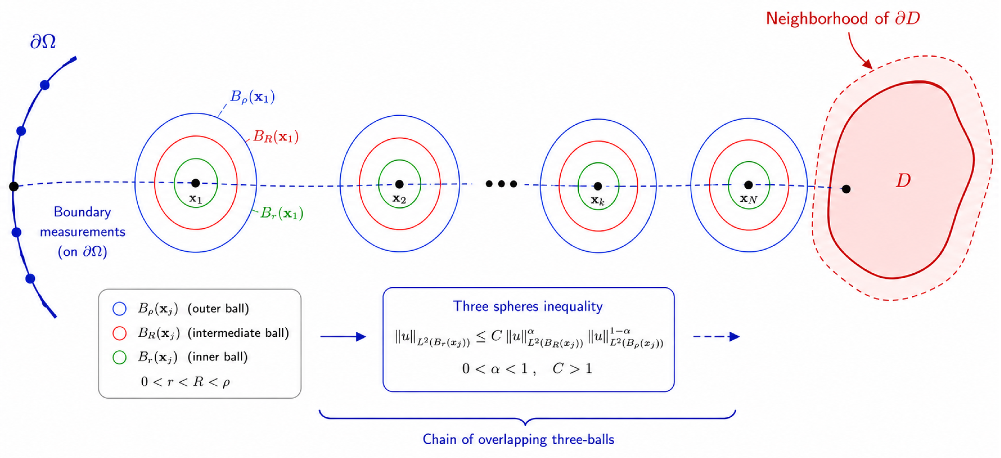
The propagation mechanism is schematically illustrated in Figure 2. More precisely, one starts from the smallness of the discrepancy of the Dirichlet-to-Neumann maps on the boundary $\parallel {\mathsf{\Lambda }}_{D_1}-{\mathsf{\Lambda }}_{D_2}\parallel \le \epsilon$, and then propagates this information toward the interior by repeated applications of three-spheres inequality. The iteration process produces estimates deteriorating exponentially with respect to the number of iterations. This exponential loss is one of the main reasons for the appearance of logarithmic stability estimates.

In discontinuous media, standard three spheres inequality are no longer sufficient. In particular, when the conductivity presents jumps across interfaces, one needs quantitative estimates capable of crossing transmission boundaries.

For this purpose, Carleman estimates adapted to discontinuous coefficients and transmission problems play a crucial role. Such estimates lead to three-region inequalities allowing the propagation of smallness across interfaces [18,19]. These techniques are particularly important in layered media and in conductivity models involving discontinuous backgrounds.

A typical outcome of the propagation-of-smallness argument is an estimate for the interaction functional $S(y,w)$ introduced in (9). When the singularities y and w approach the inclusion boundary while remaining in the exterior connected component, one obtains quantitative upper bounds for $\left|S\right(y,w\left)\right|$ in terms of the discrepancy of the boundary measurements and of the distance of the singularities from the interface.

These upper bounds are then compared with lower bounds derived from the asymptotic behavior of the fundamental solutions near $\partial D$. The balance between the deterioration produced by quantitative unique continuation and the singular behavior near the interface yields the final stability estimate.

The implementation of quantitative unique continuation arguments requires suitable geometrical constructions. In particular, one needs to connect the accessible boundary portion with neighborhoods of the unknown inclusion through paths contained in the admissible region.

Typical constructions involve chains of overlapping balls, tubular neighborhoods, and truncated cones. These geometrical devices guarantee that the radii of the balls used in the iteration procedure remain uniformly controlled.

One of the main difficulties is related to the possible presence of inaccessible regions generated by the inclusions themselves. In order to overcome this issue, suitable paths are constructed inside the connected component of the background medium whose boundary contains $\partial \mathsf{\Omega }$.

Another useful concept is the modified distance between inclusions introduced in the previous section. Singular solution arguments naturally provide estimates on points realizing the modified distance. Under the geometric assumptions stated in Proposition 1, these estimates can then be transferred to the Hausdorff distance.

Combining all the ingredients described above, one obtains inequalities relating the discrepancy of the boundary measurements to the distance between the unknown inclusions. The final logarithmic stability estimate is obtained through a balancing argument between the blow-up behavior of the singular solutions near the interface and the exponential deterioration produced by propagation of smallness.

This interplay between singular asymptotics and quantitative unique continuation constitutes the core analytical mechanism underlying most stability results for inverse inclusion problems.

4. Stability Results for Different Conductivity Models

In this section, we compare some of the main stability results available for inverse inclusion problems in electrical impedance tomography. Rather than repeating the common analytical framework described in Section 3, we focus on the features that distinguish the different settings. The comparison shows that the attainable stability modulus is determined by the interplay among several factors: The dimension and structure of the admissible geometric class, the regularity and structure of the background conductivity, and the amount and location of the available boundary measurements. These features also determine which analytical difficulties become dominant in each model. Table 1 summarizes the representative configurations discussed below.

4.1. Isotropic Conductivities

The basic model is represented by an isotropic piecewise constant conductivity of the form

$$\gamma \left(x\right)=1+(k-1){\chi }_D\left(x\right),$$

(15)

where $k>0$, $k\ne 1$, and D is the unknown inclusion. For broad admissible classes of inclusions with $C^{1,\alpha }$ boundary, logarithmic stability in the Hausdorff distance was established in [4]. This setting provides the basic example of the analytical mechanism described in Section 3: singular solutions detect the position of the unknown interface, while quantitative unique continuation propagates the discrepancy of the boundary data toward the inclusion.

The homogeneous piecewise constant model is particularly suitable for the analysis because the local transmission problem near $\partial D$ can be compared with an explicit flat-interface configuration. The main geometric difficulty is then to convert estimates obtained near points of the accessible part of the inclusion boundary into control of the full Hausdorff distance. This is precisely where the modified distance introduced in Section 2 and the geometric constructions described in Section 3 enter the argument.

The same stability mechanism can be extended to isotropic conductivities with variable coefficients,

$$\gamma \left(x\right)=a\left(x\right)+(b\left(x\right)-a\left(x\right)){\chi }_D\left(x\right),$$

(16)

Here, the background conductivity $a\left(x\right)$ is assumed to be known, and the coefficients satisfy the uniform ellipticity and regularity assumptions specified in [5] and summarized in Table 1. A quantitative nonvanishing-contrast condition across the unknown interface is also required. In particular, the admissible class is assumed to satisfy

$$|b\left(x\right)-a\left(x\right)|\ge {\kappa }_0>0\mathrm{on}\partial D,$$

in the appropriate trace sense. This assumption is essential for identifiability: without a conductivity jump across $\partial D$, the interface would not be detectable from the boundary measurements. The precise regularity and contrast assumptions depend on the conductivity class under consideration.

In this case, the main additional difficulty is the asymptotic analysis of the fundamental solution. The local transmission operator is no longer piecewise constant, and one must compare the actual fundamental solution with that of an appropriate frozen-coefficient model; see [5] for the corresponding local asymptotic estimates. Quantitative control of the error in this approximation is essential in order to retain the lower bounds generated by the singular solutions.

A further extension concerns local boundary measurements [5]. When voltages and currents are available only on an accessible portion of $\partial \mathsf{\Omega }$, the principal additional difficulty is not the singular behavior near $\partial D$, but the quantitative transfer of information from the accessible boundary to the region containing the inclusion. This requires a more careful implementation of unique continuation and suitable chains of balls connecting the measurement region with neighborhoods of $\partial D$. Under the admissibility assumptions specified in [5] and summarized in Table 1, the logarithmic stability regime persists.

4.2. Finite-Dimensional Geometric Classes and Improved Stability

The logarithmic stability estimates discussed above concern broad classes of admissible inclusions whose boundaries are allowed to vary within infinite-dimensional regularity classes. A different stability regime may arise when stronger a priori information is imposed on the geometry of the unknown inclusion. In particular, restricting the admissible set to finite-dimensional families, such as disks, polygons, or polyhedra with suitable quantitative nondegeneracy assumptions, may lead to substantially stronger stability estimates.

An important example is provided by polygonal conductivity inclusions in two dimensions. For conductivities of the form

$$\gamma \left(x\right)=1+(k-1){\chi }_P\left(x\right),$$

where $P⋐\mathsf{\Omega }$ belongs to an admissible class of polygons and the conductivity contrast is fixed, global Lipschitz stability estimates have been established in terms of the Dirichlet-to-Neumann map [10]. In particular, for two admissible polygons $P_1$ and $P_2$, one obtains an estimate of the form

$$d_H(\partial P_1,\partial P_2)\le C\parallel {\mathsf{\Lambda }}_{P_1}-{\mathsf{\Lambda }}_{P_2}\parallel .$$

This result should be contrasted with the logarithmic modulus obtained for general $C^{1,\alpha }$ inclusions. The improvement is closely related to the finite-dimensional character of the admissible geometric class and to the quantitative control of its parameters.

The polygonal setting has also been investigated in the presence of a discontinuous background. In particular, Lipschitz stability has been established for polygonal conductivity inclusions in a two-dimensional layered medium [11]. Here, the main difficulty is different from that of the homogeneous case: perturbations of the polygonal geometry must be analyzed in the presence of fixed transmission interfaces. The derivation of quantitative estimates therefore requires simultaneous control of the geometric perturbation and of the transmission structure of the background medium.

A further significant development concerns polyhedral inclusions in three dimensions. Lipschitz stability for polyhedral conductivity inclusions from a local Dirichlet-to-Neumann map has been established in [9]. This shows that the Lipschitz regime can persist in three dimensions and even when measurements are restricted to an accessible portion of the exterior boundary. The analysis is nevertheless considerably more delicate, since faces, edges, vertices, and their mutual geometric relations must be controlled quantitatively.

Finite-dimensional geometric information may also improve stability when the amount of boundary data is strongly reduced, although the resulting modulus need not be Lipschitz. For disk-shaped inclusions, Hölder stability can be obtained from a single boundary measurement under stronger a priori assumptions [13]. For convex polygonal inclusions, logarithmic stability has been established from a single partial boundary measurement [12].

More recent developments have further reduced the amount of boundary information required for stable determination. Within a general framework for inverse problems on low-dimensional manifolds, Alberti, Arroyo and Santacesaria obtained Lipschitz stability from a finite number of measurements for piecewise constant conductivities with an unknown triangular inclusion [14]. This provides a direct connection between finite-dimensional geometric parametrization and finite-measurement stability.

Hanke subsequently proved Lipschitz stability for a planar polygonal conductivity inclusion from only two suitable Cauchy data pairs [15]; in the insulating case, a single nontrivial Cauchy pair is sufficient. More recent work has also addressed the simultaneous determination of polygonal geometry and an unknown constant conductivity value [16], while logarithmic stability for convex polyhedral inclusions in three dimensions from a single boundary measurement has recently been established in [17]. The latter two contributions are currently available as preprints. These examples show that finite-dimensionality alone does not determine the stability modulus: the amount and location of the available boundary information are equally important. The results summarized in Table 1 therefore suggest that geometric complexity and measurement richness must be considered jointly when comparing stability regimes.

4.3. Anisotropic Conductivities

A substantially different difficulty arises in anisotropic media. We refer here specifically to the stability result of Di Cristo and Ren [6]. The model considered in that work is based on a known anisotropic background represented by a symmetric matrix-valued function $A\left(x\right)$, while the conductivity inside the inclusion is of the form $kA\left(x\right)$. Accordingly, the conductivity can be written as

$${\sigma }_D\left(x\right)=A\left(x\right)+(k-1)A\left(x\right){\chi }_D\left(x\right).$$

(17)

It is useful to distinguish between the general model described in the introductory formulation of [6] and the precise setting of its stability theorem. While the conductivity contrast is initially introduced in a more general form, the logarithmic stability result summarized here is proved for a fixed scalar parameter $k>0$, $k\ne 1$, which is included among the a priori data. Thus, the result concerns the determination of the geometry of D within a prescribed anisotropic background and for a prescribed nonvanishing conductivity contrast; it does not address the simultaneous recovery of the inclusion and an independently unknown anisotropic conductivity.

More precisely, the background matrix $A\left(x\right)$ is assumed to be known, symmetric, and Lipschitz continuous in $\mathsf{\Omega }$, with a uniform bound

$${\parallel A\parallel }_{C^{0,1}\left(\mathsf{\Omega }\right)} \le \mathcal{A},$$

and it satisfies the uniform ellipticity condition

$${\lambda }_0{\left|\xi \right|}^2\le A\left(x\right)\xi ·\xi \le {\mathsf{\Lambda }}_0{\left|\xi \right|}^2,x\in \mathsf{\Omega },\xi \in {\mathbb{R}}^n,$$

for fixed constants $0<{\lambda }_0\le {\mathsf{\Lambda }}_0$.

The domain and the inclusion boundaries are assumed to be of class $C^{1,\alpha }$ with uniform constants; moreover, D stays at a prescribed positive distance from $\partial \mathsf{\Omega }$ and $\mathsf{\Omega }\setminus \overline{D}$ is connected. The dimension, the contrast k, the geometric regularity parameters, the separation distance, and the ellipticity and Lipschitz bounds for A constitute the a priori data in the stability estimate.

Under these assumptions, Di Cristo and Ren prove a logarithmic stability estimate for the Hausdorff distance between two admissible inclusions in terms of the operator norm of the corresponding Dirichlet-to-Neumann maps [6]. The principal additional difficulty with respect to the isotropic piecewise constant case is the asymptotic analysis of the fundamental solutions near $\partial D$.

At sufficiently small scales, the anisotropic operator is compared with a frozen-coefficient transmission problem determined by the matrix $A\left(x_0\right)$ at a point $x_0\in \partial D$. Let ${\mathsf{\Gamma }}_D$ denote the fundamental solution of the actual anisotropic conductivity operator and let ${\mathsf{\Gamma }}_0$ denote the fundamental solution of the corresponding flat-interface problem with the coefficient frozen at $A\left(x_0\right)$.

The precise comparison estimates used in the stability argument are given in Theorem 4.1 of [6]. In the local coordinates and notation of that result, one has

$$|{\mathsf{\Gamma }}_D(x,y)-{\mathsf{\Gamma }}_0(x,y)|\le {\displaystyle \frac{C}{r_1^{\alpha }}}{|x-y|}^{2-n+\alpha },$$

(18)

and

$$|{\nabla }_x{\mathsf{\Gamma }}_D(x,y)-{\nabla }_x{\mathsf{\Gamma }}_0(x,y)|\le {\displaystyle \frac{C}{r_1^{{\alpha }^2}}}{|x-y|}^{1-n+{\alpha }^2},$$

(19)

where $C>0$ depends only on the a priori data and $r_1$ is the local geometric scale introduced in Theorem 4.1 of [6].

These estimates provide the anisotropic counterpart of the interface asymptotics discussed in Section 3. Their significance is that the leading singular behavior still contains quantitative information on the position of the interface, but now relative to the local geometry induced by the anisotropic coefficient. Thus, while the propagation-of-smallness mechanism remains conceptually similar to the isotropic case, the construction and comparison of the singular solutions constitute the genuinely model-dependent part of the analysis. The identifiability assumptions stated above, together with the nonvanishing contrast across the inclusion boundary, are also essential in order to distinguish the inclusion from the known anisotropic background.

4.4. Layered Media

Inverse inclusion problems in layered media introduce a different source of difficulty: the background conductivity itself is discontinuous across known interfaces. A representative two-layer model is

$$\gamma \left(x\right)=c_1+(c_2-c_1){\chi }_{{\mathsf{\Omega }}_{+}}+(k-c_2){\chi }_D,$$

(20)

where ${\mathsf{\Omega }}_{+}$ denotes one of the layers and D is the unknown inclusion.

Let $\mathsf{\Sigma }$ denote a transmission interface and fix a unit normal vector $\nu$ on $\mathsf{\Sigma }$, oriented from the “−” side toward the “+” side. The transmission conditions express continuity of the electric potential and of the normal current flux:

$$u^{+}=u^{-},({\gamma }^{+}\nabla u^{+})·\nu =({\gamma }^{-}\nabla u^{-})·\nu \mathrm{on}\mathsf{\Sigma }.$$

(21)

Here, $u^{\pm }$ and ${\gamma }^{\pm }$ denote the traces of the potential and the conductivity from the two sides of the interface, respectively.

Consequently, quantitative information originating at the exterior boundary must be propagated through regions in which the coefficients may jump. Standard interior three-sphere inequality cannot simply be iterated across such interfaces.

This difficulty motivates the use of Carleman estimates adapted to elliptic operators with discontinuous leading coefficients and of the associated three-region inequalities [18,19]. These estimates provide quantitative unique continuation across transmission interfaces and make it possible to extend the propagation-of-smallness mechanism to stratified backgrounds.

Under the geometric, separation, and contrast assumptions specified in [7] and summarized in Table 1, logarithmic stability estimates for the determination of the inclusion have been obtained.

The analysis becomes still more delicate when the conductivity coefficients inside the layers or the inclusion vary spatially [8]. In this case, local frozen-coefficient asymptotics must be combined with quantitative unique continuation across discontinuous interfaces. The relevant assumptions therefore involve not only the geometry of D, but also the regularity, ellipticity, and contrast of the coefficients in the different regions.

The finite-dimensional theory discussed above shows that the layered structure does not by itself force logarithmic stability. Indeed, for the admissible polygonal class considered in [11], Lipschitz stability can be recovered in a two-dimensional layered medium. This comparison provides another indication that the stability modulus is determined jointly by the complexity of the unknown geometry, the structure of the background medium, and the available measurements.

The comparison above also shows that the principal analytical obstruction is model-dependent. For variable isotropic coefficients, the main additional ingredient is a quantitative comparison of the fundamental solution with a local frozen-coefficient transmission model. In anisotropic media, the leading singular behavior must instead be analyzed relative to the local geometry induced by the matrix coefficient. Layered backgrounds introduce a different difficulty: quantitative information must cross known transmission interfaces, requiring interface-adapted Carleman estimates and three-region inequalities. Reduced boundary measurements do not primarily alter the local singular structure, but increase the difficulty of propagating information from the accessible boundary to the unknown interface.

The available results therefore suggest that the stability modulus should not be viewed as a property of the conductivity equation alone. It reflects the combined effect of the complexity of the admissible geometry, the regularity and structure of the coefficients, and the amount of boundary information available. Some assumptions play structurally different roles: nonvanishing contrast is required for identifiability of the interface, regularity assumptions permit quantitative local asymptotics, separation conditions prevent interaction between distinct transmission structures, and connectivity assumptions allow boundary information to be propagated toward the unknown inclusion. Table 1 summarizes how these ingredients enter the representative results discussed above.

Table 1. Representative stability results for inverse inclusion problems. The assumptions reported in the table summarize the admissible classes appearing in the corresponding stability results.

Reference	Inclusion Geometry	Background Medium	Measurements	Dim.	Main a Priori Assumptions	Stability
Alessandrini–Di Cristo [4]	$C^{1,\alpha }$ inclusion, possibly disconnected	Homogeneous isotropic	Full Dirichlet-to-Neumann map	$n\ge 2$	$\partial \mathsf{\Omega }$ and $\partial D$ of class $C^{1,\alpha }$ with uniform constants; $\mathrm{dist}(D,\partial \mathsf{\Omega })\ge \delta$; $\mathsf{\Omega }\setminus \overline{D}$ connected; fixed known contrast $k>0$, $k\ne 1$	Logarithmic
Di Cristo [5]	$C^{1,\alpha }$ inclusion	Known variable isotropic background	Local boundary measurements	$n\ge 2$	Uniform $C^{1,\alpha }$ geometric bounds; inclusion separated from $\partial \mathsf{\Omega }$; connected exterior region; known regular background; quantitative nonvanishing contrast across $\partial D$; measurements on a prescribed accessible portion of the boundary	Logarithmic
Di Cristo–Ren [6]	$C^{1,\alpha }$ inclusion	Known anisotropic background	Full Dirichlet-to-Neumann map	$n\ge 2$	$A\left(x\right)$ known, symmetric, Lipschitz and uniformly elliptic; $\partial \mathsf{\Omega },\partial D\in C^{1,\alpha }$ with uniform constants; $\mathrm{dist}(D,\partial \mathsf{\Omega })\ge \delta$; $\mathsf{\Omega }\setminus \overline{D}$ connected; fixed scalar contrast $k>0$, $k\ne 1$	Logarithmic
Di Cristo–Ren [7]	$C^{1,\alpha }$ inclusion	Known piecewise constant layered isotropic medium	Full Dirichlet-to-Neumann map	$n\ge 2$	Known layer conductivities and transmission interfaces; $\partial D\in C^{1,\alpha }$ with uniform constants; positive distance between D and the layer interfaces and between D and $\partial \mathsf{\Omega }$; connected exterior region; fixed nonvanishing contrast between the inclusion and the surrounding layer	Logarithmic
Di Cristo–Ren [8]	$C^{1,\alpha }$ inclusion	Known stratified background with variable coefficients	Full Dirichlet-to-Neumann map	$n\ge 2$	Known layer coefficients $a_1,a_2\in C^{0,1}$, unknown inclusion coefficient $b\in C^{\alpha }$; uniform ellipticity; $|a_2-b|\ge {\eta }_0>0$ in the inclusion layer; $\partial D,\partial \mathsf{\Omega }\in C^{1,\alpha }$; layer interface of class $C^2$; positive separation of D from the interface and of the interface from $\partial \mathsf{\Omega }$; connected exterior	Logarithmic
Triki–Tsou [13]	Disk	Homogeneous isotropic	Single Cauchy pair	2	$\mathsf{\Omega }$ simply connected and Lipschitz; D a disk compactly contained in $\mathsf{\Omega }$; fixed known contrast $k>0$, $k\ne 1$; arbitrary nonzero Neumann datum satisfying the compatibility condition	Hölder
Liu–Tsou [12]	Convex polygon	Homogeneous isotropic	Single partial boundary measurement	2	Piecewise constant conductivity with fixed nonzero contrast; convex polygonal support satisfying quantitative geometric nondegeneracy assumptions; measurement restricted to an accessible boundary portion	Logarithmic
Beretta–Francini [10]	Simple polygon, not necessarily convex	Homogeneous isotropic	Full Dirichlet-to-Neumann map	2	Polygon has at most $N_0$ sides, each of length at least $d_0$; uniform Lipschitz constants; vertex angles bounded away from 0, $\pi$ and $2\pi$; $\mathrm{dist}(P,\partial \mathsf{\Omega })\ge d_0$; fixed known contrast $k>0$, $k\ne 1$	Lipschitz
Beretta–Francini–Vessella [11]	Simple polygon, not necessarily convex	Known piecewise constant layered medium	Full Dirichlet-to-Neumann map	2	At most $N_0$ sides of length at least $d_0$; uniform Lipschitz and angle nondegeneracy conditions; $\mathrm{dist}(P,\partial \mathsf{\Omega })\ge d_0$; every vertex stays at least $d_0/2$ from the known layer interfaces; layer widths bounded below; known layer conductivities; $|k-{\gamma }_i|\ge c_0>0$	Lipschitz
Aspri–Beretta–Francini–Vessella [9]	Nondegenerate polyhedron	Homogeneous isotropic	Local Dirichlet-to-Neumann map on $\mathsf{\Sigma }$	3	$\mathrm{dist}(D,\partial \mathsf{\Omega })\ge r_0$; uniform lower bounds on edge lengths and face size; face and dihedral angles bounded away from degeneracy; $\mathsf{\Omega }\setminus D$ connected with uniformly Lipschitz boundary; $\min \{k,|k-1\left|\right\}\ge {\kappa }_0$; accessible portion $\mathsf{\Sigma }$ contains a boundary neighborhood of size at least $r_0$	Lipschitz
Hanke [15]	Admissible polygon with fixed number of vertices	Homogeneous isotropic	Two Cauchy data pairs	2	Smooth outer boundary; fixed known conductivity $k>0$, $k\ne 1$; polygonal inclusion compactly contained in $\mathsf{\Omega }$; vertices uniformly separated from nonadjacent edges and from $\partial \mathsf{\Omega }$; interior angles uniformly bounded away from 0, $\pi$ and $2\pi$; two probing currents satisfying Seo’s nondegeneracy condition	Lipschitz

Table 1. Representative stability results for inverse inclusion problems. The assumptions reported in the table summarize the admissible classes appearing in the corresponding stability results.

Reference	Inclusion Geometry	Background Medium	Measurements	Dim.	Main a Priori Assumptions	Stability
Alessandrini–Di Cristo [4]	$C^{1,\alpha }$ inclusion, possibly disconnected	Homogeneous isotropic	Full Dirichlet-to-Neumann map	$n\ge 2$	$\partial \mathsf{\Omega }$ and $\partial D$ of class $C^{1,\alpha }$ with uniform constants; $\mathrm{dist}(D,\partial \mathsf{\Omega })\ge \delta$; $\mathsf{\Omega }\setminus \overline{D}$ connected; fixed known contrast $k>0$, $k\ne 1$	Logarithmic
Di Cristo [5]	$C^{1,\alpha }$ inclusion	Known variable isotropic background	Local boundary measurements	$n\ge 2$	Uniform $C^{1,\alpha }$ geometric bounds; inclusion separated from $\partial \mathsf{\Omega }$; connected exterior region; known regular background; quantitative nonvanishing contrast across $\partial D$; measurements on a prescribed accessible portion of the boundary	Logarithmic
Di Cristo–Ren [6]	$C^{1,\alpha }$ inclusion	Known anisotropic background	Full Dirichlet-to-Neumann map	$n\ge 2$	$A\left(x\right)$ known, symmetric, Lipschitz and uniformly elliptic; $\partial \mathsf{\Omega },\partial D\in C^{1,\alpha }$ with uniform constants; $\mathrm{dist}(D,\partial \mathsf{\Omega })\ge \delta$; $\mathsf{\Omega }\setminus \overline{D}$ connected; fixed scalar contrast $k>0$, $k\ne 1$	Logarithmic
Di Cristo–Ren [7]	$C^{1,\alpha }$ inclusion	Known piecewise constant layered isotropic medium	Full Dirichlet-to-Neumann map	$n\ge 2$	Known layer conductivities and transmission interfaces; $\partial D\in C^{1,\alpha }$ with uniform constants; positive distance between D and the layer interfaces and between D and $\partial \mathsf{\Omega }$; connected exterior region; fixed nonvanishing contrast between the inclusion and the surrounding layer	Logarithmic
Di Cristo–Ren [8]	$C^{1,\alpha }$ inclusion	Known stratified background with variable coefficients	Full Dirichlet-to-Neumann map	$n\ge 2$	Known layer coefficients $a_1,a_2\in C^{0,1}$, unknown inclusion coefficient $b\in C^{\alpha }$; uniform ellipticity; $|a_2-b|\ge {\eta }_0>0$ in the inclusion layer; $\partial D,\partial \mathsf{\Omega }\in C^{1,\alpha }$; layer interface of class $C^2$; positive separation of D from the interface and of the interface from $\partial \mathsf{\Omega }$; connected exterior	Logarithmic
Triki–Tsou [13]	Disk	Homogeneous isotropic	Single Cauchy pair	2	$\mathsf{\Omega }$ simply connected and Lipschitz; D a disk compactly contained in $\mathsf{\Omega }$; fixed known contrast $k>0$, $k\ne 1$; arbitrary nonzero Neumann datum satisfying the compatibility condition	Hölder
Liu–Tsou [12]	Convex polygon	Homogeneous isotropic	Single partial boundary measurement	2	Piecewise constant conductivity with fixed nonzero contrast; convex polygonal support satisfying quantitative geometric nondegeneracy assumptions; measurement restricted to an accessible boundary portion	Logarithmic
Beretta–Francini [10]	Simple polygon, not necessarily convex	Homogeneous isotropic	Full Dirichlet-to-Neumann map	2	Polygon has at most $N_0$ sides, each of length at least $d_0$; uniform Lipschitz constants; vertex angles bounded away from 0, $\pi$ and $2\pi$; $\mathrm{dist}(P,\partial \mathsf{\Omega })\ge d_0$; fixed known contrast $k>0$, $k\ne 1$	Lipschitz
Beretta–Francini–Vessella [11]	Simple polygon, not necessarily convex	Known piecewise constant layered medium	Full Dirichlet-to-Neumann map	2	At most $N_0$ sides of length at least $d_0$; uniform Lipschitz and angle nondegeneracy conditions; $\mathrm{dist}(P,\partial \mathsf{\Omega })\ge d_0$; every vertex stays at least $d_0/2$ from the known layer interfaces; layer widths bounded below; known layer conductivities; $|k-{\gamma }_i|\ge c_0>0$	Lipschitz
Aspri–Beretta–Francini–Vessella [9]	Nondegenerate polyhedron	Homogeneous isotropic	Local Dirichlet-to-Neumann map on $\mathsf{\Sigma }$	3	$\mathrm{dist}(D,\partial \mathsf{\Omega })\ge r_0$; uniform lower bounds on edge lengths and face size; face and dihedral angles bounded away from degeneracy; $\mathsf{\Omega }\setminus D$ connected with uniformly Lipschitz boundary; $\min \{k,|k-1\left|\right\}\ge {\kappa }_0$; accessible portion $\mathsf{\Sigma }$ contains a boundary neighborhood of size at least $r_0$	Lipschitz
Hanke [15]	Admissible polygon with fixed number of vertices	Homogeneous isotropic	Two Cauchy data pairs	2	Smooth outer boundary; fixed known conductivity $k>0$, $k\ne 1$; polygonal inclusion compactly contained in $\mathsf{\Omega }$; vertices uniformly separated from nonadjacent edges and from $\partial \mathsf{\Omega }$; interior angles uniformly bounded away from 0, $\pi$ and $2\pi$; two probing currents satisfying Seo’s nondegeneracy condition	Lipschitz

5. Open Problems and Perspectives

The results reviewed above also make it possible to delimit more precisely which aspects of inverse inclusion stability remain unresolved. Several configurations that were formerly regarded as major obstacles (including polygonal and polyhedral geometries, local measurements, anisotropic backgrounds, and layered media) are now covered by quantitative stability results under appropriate structural assumptions. The remaining difficulties are therefore not simply extensions to “more general” models, but concern specific mechanisms for which the available analytical tools cease to be uniform or sufficiently precise.

In the following, we distinguish these genuinely open stability questions from settings for which substantial uniqueness, forward, or reconstruction theory is already available.

Partial Boundary Measurements

One of the most relevant issues from the viewpoint of applications concerns partial data problems. In many practical situations, measurements are available only on a limited portion of the boundary and the inaccessible part may even be large.

Although logarithmic stability estimates have been obtained in several local measurement settings, many questions remain open. In particular, it would be interesting to understand whether sharper quantitative estimates can be derived under additional geometrical assumptions and to determine the minimal amount of boundary information required for stable reconstruction.

Another important aspect concerns the geometry of the accessible boundary portion. The propagation of smallness arguments strongly depend on the possibility of connecting the measurements region to the unknown inclusion through suitable paths. Understanding the optimal geometrical assumptions for quantitative continuation remains an interesting open problem.

Low-Regularity and Nonsmooth Geometries

Most stability results for general classes of inclusions rely on a priori regularity assumptions on the unknown interface, typically of class $C^{1,\alpha }$. Such assumptions play an important role both in the local asymptotic analysis of singular solutions and in the quantitative unique continuation arguments used to propagate information toward the inclusion.

Substantial progress has nevertheless been achieved for specific nonsmooth finite-dimensional classes, most notably polygonal and polyhedral inclusions; see Section 4.2 and the references therein. These results rely on quantitative nondegeneracy assumptions and therefore do not extend directly to arbitrary nonsmooth interfaces.

A genuinely open direction is to understand quantitative stability for broader infinite-dimensional classes of low-regularity inclusions, for example, general Lipschitz interfaces or boundaries exhibiting cusps and other geometric singularities without an a priori finite-dimensional parametrization. In such settings, the local behavior of singular solutions may differ substantially from that associated with smooth or polygonal interfaces, and the geometric control required in propagation-of-smallness arguments may deteriorate. Determining which regularity and structural assumptions are sufficient for quantitative reconstruction, and identifying the corresponding optimal modulus of stability, remain challenging open problems.

Inclusions Approaching Background Interfaces

Another challenging situation arises when the inclusion approaches or intersects interfaces of the background medium. In layered media, most existing results assume that the inclusion remains at positive distance from the transmission interfaces.

The analysis of touching configurations appears considerably more difficult. In particular, the asymptotic estimates used in the stability arguments discussed above are not directly uniform when the unknown inclusion approaches a background transmission interface. The local geometry may generate complex transmission phenomena which are not captured by the standard flat-interface approximations.

This issue is especially relevant in applications involving stratified or composite materials, where inclusions may naturally appear close to interfaces separating different layers.

A major difficulty comes from the fact that most of the available asymptotic estimates for singular solutions rely on the possibility of approximating the inclusion boundary and the transmission interface independently.

When the inclusion approaches the interface, these two geometrical structures interact at the same scale and the corresponding model transmission problems are no longer sufficient to describe the local behavior of the fundamental solutions.

Simultaneous Recovery of Inclusion Geometry and Background

Most of the stability results discussed in this review assume that the background conductivity is known. This assumption should not be confused with the much broader inverse conductivity problem, for which an extensive body of literature on uniqueness and stability for unknown coefficients is available.

The specific issue relevant to the present review is more restricted. Consider, for instance, a discontinuous conductivity of the form

$$\gamma \left(x\right)=a\left(x\right)+(b\left(x\right)-a\left(x\right)){\chi }_D\left(x\right),$$

where not only the inclusion D but also the background coefficient $a\left(x\right)$ is unknown and is allowed to vary independently within a prescribed admissible class. The inverse problem then involves the simultaneous determination of the geometry of the discontinuity set $\partial D$ and of an independently unknown background coefficient from the same boundary measurements.

This joint recovery problem differs substantially from both the standard inverse conductivity problem, in which one seeks to determine a coefficient without an independently parametrized unknown interface, and the inverse inclusion problems considered in the preceding sections, where the background is prescribed. In the latter setting, knowledge of the background is used in the construction of comparison fundamental solutions and in the derivation of the local asymptotics near $\partial D$. If the background is also unknown, perturbations of the coefficient and perturbations of the inclusion geometry may contribute simultaneously to the boundary data, and additional structural assumptions are required to separate these effects.

We emphasize that quantitative stability for the recovery of unknown conductivity coefficients has been extensively investigated in other settings. Classical continuous dependence results for scalar conductivities go back to [26], while Lipschitz stability has been established for finite-dimensional classes of piecewise constant conductivities [27]. The issue considered here is therefore not stability for an unknown conductivity per se, but the coupled recovery of an independently unknown background coefficient and an unknown inclusion geometry.

A relevant open direction is therefore to determine quantitative stability for such simultaneous recovery problems under precisely specified admissible classes for both a and D. In particular, it would be interesting to identify conditions under which the geometric component of the reconstruction admits a quantitative stability estimate and to understand how its modulus depends on the independent uncertainty in the background coefficient. We do not intend this statement as a claim that stability for general unknown conductivities is open, but rather as a question concerning this specific coupled geometry–coefficient recovery problem.

Closely Spaced and Touching Components

The presence of several connected components should not in itself be regarded as an unresolved extension of the inverse inclusion problem. For instance, the logarithmic stability result of Alessandrini and Di Cristo [4] allows the unknown inclusion to be disconnected. Moreover, multiple-inclusion configurations have been extensively studied from the viewpoints of forward analysis, detection, asymptotic expansions, and numerical reconstruction.

A substantially more delicate regime arises when distinct components become arbitrarily close or touch. The forward conductivity problem in such configurations has been the subject of extensive analysis. In the perfect and insulated conductivity limits, quantitative estimates describe the possible blow-up of the electric field in the narrow region between nearby inclusions [28]. Related asymptotic analyses are also available for nearly touching inclusions with nonsmooth geometries [29]. These results show that the interaction between neighboring interfaces may change the local singular structure substantially.

The open issue relevant to the present review is therefore more specific: to obtain stability estimates for the inverse geometric determination of several inclusions that remain uniform, or whose deterioration can be quantified sharply, as the minimal separation between distinct components tends to zero. Most singular-solution stability arguments rely on geometric a priori parameters that control the admissible interfaces and the regions through which smallness is propagated. When two unknown interfaces approach one another, the corresponding constants may deteriorate and the local asymptotic models used for an isolated interface may cease to provide a uniform description.

It would therefore be interesting to determine the precise dependence of inverse stability estimates on the minimal separation between components, to identify geometric classes for which uniform estimates remain possible, and to understand the limiting situation in which distinct components touch. These questions concern quantitative inverse stability and should be distinguished from the substantial existing theory for the corresponding forward conductivity problems.

Reconstruction Procedures

The stability estimates discussed in this review are primarily analytical results describing the continuous dependence of the unknown inclusion on the boundary measurements. A distinct question is how such estimates can be translated into effective reconstruction procedures in the presence of measurement noise.

From a computational viewpoint, several issues remain relevant, including the convergence rates of regularization methods, the sensitivity of reconstruction algorithms to noise, and the derivation of quantitative error bounds for iterative schemes. In particular, it is important to understand to what extent the stability modulus available for a given admissible class can be reflected in convergence rates and stopping criteria for practical reconstruction methods.

Bridging the gap between analytical stability theory and computational reconstruction therefore remains an important direction, especially for complex conductivity models and limited-data configurations.

Stability versus Instability

A fundamental theoretical question concerns the optimal modulus of continuity for the inverse map. Exponential instability results for specific infinite-dimensional admissible classes show that logarithmic-type stability is essentially optimal in those settings [3]. By contrast, the results surveyed in Section 4 show that stronger moduli may occur under additional geometric and measurement constraints.

A broader objective is therefore to identify which structural features of the admissible class determine the optimal stability modulus, rather than to associate a single stability regime with inverse inclusion problems as a whole.

Final Remarks

The study of inverse inclusion problems continues to be a very active research area at the intersection of analysis, partial differential equations, inverse problems, and applied mathematics. Although quantitative stability estimates are now available in several settings, challenging questions remain concerning the extension and optimality of such estimates for broader geometric classes, interacting interfaces, and strongly reduced measurement configurations.

The developments reviewed here indicate that no single analytical mechanism or stability modulus characterizes inverse inclusion problems as a whole. The singular-solution and quantitative unique continuation framework remains a common backbone, but its implementation depends strongly on the geometry of the admissible class, the coefficient structure, and the measurement configuration. A central direction for future research is therefore not merely to extend existing estimates to broader models, but to identify which structural assumptions are genuinely necessary and which stability moduli are optimal for each admissible class.