Asymptotic Theory for Kernel Density Estimation Under Dependent Length-Biased Sampling

Abstract

We establish an asymptotic theory for the Jones inverse-weighted kernel density estimator when length-biased observations form a strictly stationary short-range dependent sequence. The statistical difficulty is intrinsically composite: reciprocal weighting is singular at the origin, the normalizing mean is estimated from the same dependent sample, kernel localization shrinks with the bandwidth, and the centered summands form a row-wise stationary triangular array whose envelope diverges at rate $h_n^{-1}$. Under a non-negative compactly supported Lipschitz kernel, an inverse-moment condition, geometric $\alpha$-mixing, local regularity of the target density, and uniform local bounds on lagged bivariate densities, we prove strong uniform consistency on compact subsets of $(0,\infty )$ and, separately, the uniform stochastic bound $O_{\mathbb{P}}\{h_n^2+{(\log n/\left(n{h}_n\right))}^{1/2}\}$. A covariance-localization argument shows that the scaled serial-covariance contribution is $O\left\{h_n\log (1/h_n)\right\}=o\left(1\right)$, so the first-order pointwise variance coincides with that of the corresponding independent length-biased estimator. Pointwise and finite-dimensional Gaussian limits are obtained by an explicit big-block/small-block argument with off-diagonal covariance control. The ratio normalization is treated directly: its variance contribution, its product with the localized fluctuation, and its cross-covariance with that fluctuation are all negligible at the $\sqrt{n{h}_n}$ scale. We further derive first-order AMSE and AMISE criteria, their oracle bandwidths, and feasible pointwise studentization under undersmoothing. The numerical study separates oracle from data-driven bandwidth selection, evaluates full-ratio HAC and moving-block corrections, examines a Frank-copula Markov robustness design, and benchmarks the Jones estimator against an alternative length-biased estimator. The simulations support the first-order theory while demonstrating that persistent short-range dependence can remain consequential for finite-sample uncertainty.

1. Introduction

Length-biased sampling is a canonical instance of informative observation: the probability that an individual, object, duration, or lifetime enters the sample is proportional to its magnitude. The mechanism already appears in the stereological work of [1], where larger particles are more likely to intersect a sampling plane, and it was subsequently placed on a systematic statistical footing in [2,3,4]. More generally, weighted distributions arise naturally in renewal theory, survival analysis, reliability, epidemiology, biomedical studies, genetics, econometrics, and cross-sectional sampling; see, among others, refs. [5,6,7,8,9,10,11] and the survey [12]. In each of these settings, the observation law differs systematically from the scientific target so that the statistical problem is not one of ordinary smoothing under a misspecified marginal distribution but of recovering a latent target law through a structurally biased sampling operator.

Let $X\ge 0$ denote the variable of scientific interest, with distribution function F, density f, and finite positive mean $\mu ={\int }_0^{\infty }xdF\left(x\right)$. Under length-biased sampling, the observed variable Y has density

$$g\left(t\right)={\displaystyle \frac{tf\left(t\right)}{\mu }},t>0.$$

(1)

Thus, the inferential object is f, whereas the observed process has one-dimensional marginal density g. The mapping $f\mapsto g$ is multiplicative in the state variable, and its inversion necessarily introduces the reciprocal weight $t^{-1}$. This inverse weighting is therefore not an ad hoc bias correction: it is the exact Radon–Nikodym mechanism by which the target law is reconstructed from its length-biased image.

The probabilistic relevance of dependence is particularly transparent in two classical examples. In renewal theory, inspection at a randomly selected epoch favors long renewal intervals and produces the inspection paradox together with the equilibrium relations among total, backward, and forward recurrence times; see [13]. In survival analysis, prevalent-cohort sampling over-represents long survival durations and is closely related, under stationarity, to random left truncation [9]. The corresponding censored setting has generated a substantial literature on unbiased survivor estimation, likelihood-based inference, regression, and semiparametric efficiency; see, for example, refs. [14,15,16,17,18]. Such examples also show why independence may be an unrealistic structural assumption: length-biased observations can inherit temporal, spatial, cluster, or longitudinal dependence from the underlying sampling mechanism.

This distinction has direct inferential consequences. In a prevalent-cohort study assembled in temporally clustered enrollment waves, or in a renewal/reliability monitor whose inspected durations are serially correlated, treating the length-biased observations as independent can leave the inverse-weighted point estimator qualitatively reasonable while materially understating finite-sample uncertainty. In particular, the lagged covariance of the localized inverse-weighted terms can remain numerically important even when it is asymptotically of smaller order. A principal purpose of the present analysis is therefore to identify exactly when the classical independent first-order variance is recovered and, equally importantly, why that first-order equivalence does not guarantee well-calibrated finite-sample studentization under stronger persistence.

The present paper concerns kernel density estimation in this dependent length-biased setting. For ordinary direct observations, kernel density estimation originates with [19,20], with foundational consistency results developed in [21,22,23,24,25,26,27,28]. If a conventional kernel estimator is applied directly to length-biased observations, however, it estimates g rather than f. The sampling distortion must therefore be inverted explicitly. Early kernel methods for length-biased density estimation include [29]; the estimator of [30] uses the natural reciprocal weighting and is closely connected with an inverse-weighted empirical reconstruction of the target distribution. Subsequent developments include the rejection-sampling approach of [31], the minimax analysis of [32], Bayesian bandwidth selection in [33], and strong uniform consistency and asymptotic normality for independent length-biased observations in [34].

Recent work has continued to develop adjacent parts of this literature. Borrajo, González–Manteiga, and Martínez–Miranda [35] provided dedicated bootstrap, cross-validation, and rule-of-thumb bandwidth selection procedures for kernel density estimation with length-biased data. Kakizawa [36] developed asymmetric-kernel density estimators for biased/length-biased non-negative data and established MISE, strong consistency, and asymptotic-normality results in the independent setting. Arvanitis [37] derived non-asymptotic concentration results for ordinary kernel density estimators under uniform ($\varphi$-)mixing, a dependence framework distinct from the geometrically strong-mixing inverse-weighted array studied here. Recent work also includes biased-sampling copula-density estimation [38], kernel estimation of mean residual lifetime under length bias [39], a Berry–Esseen bound for a smoothed length-biased distribution estimator [40], kernel estimation of varextropy under length-biased sampling [41], non-parametric residual-extropy estimation under length-biased sampling with a kernel confidence interval [42], simulation from weighted distributions [43], and a recent general treatment of non-parametric function estimation under biased sampling [44]. Their results are complementary rather than substitutes for the present argument: within the literature reviewed here, we have not identified a result that supplies the specific combination used below: a Jones-type random ratio normalizer, geometric $\alpha$-mixing, local covariance localization for the singular inverse-weighted kernel array, and a row-wise big-block/small-block central limit theorem. This is a literature-positioning statement, not a claim that no other related result can exist. This comparison is intentionally narrow; we do not claim that the present paper exhausts the broader literature on dependent or weighted non-parametric estimation, see

Table 1. Positioning of the present contribution relative to closely related work. “Feasible BW” denotes a data-driven bandwidth rule; “dependent inference” denotes an inference procedure explicitly adjusted for serial dependence. Entries are intentionally conservative.

Reference	Estimator/Setting	Dependence	Feasible BW	Principal Relevance Here
Jones (1991) [30]	inverse-weighted length-biased KDE	independent	no	classical ratio estimator and random normalizer
Borrajo et al. (2017) [35]	Jones-type length-biased KDE	independent	yes	rule-of-thumb, cross-validation and bootstrap bandwidth selection
Ajami et al. (2013) [34]	length-biased KDE	independent	no	strong consistency and pointwise asymptotic normality
Kakizawa (2024) [36]	asymmetric-kernel biased-data KDE	independent	not central	recent independent biased-data asymptotics
Arvanitis (2023) [37]	ordinary KDE under mixing	dependent	no	concentration under a dependence framework distinct from the present inverse-weighted array
Present paper	Jones-type length-biased KDE	geometric $\alpha$-mixing	numerically studied	dependent asymptotic theory, covariance localization, feasible bandwidth comparison, and finite-sample dependence-aware inference study

.

The comparison is intentionally restricted to features that bear directly on the present contribution. The feasible selectors and dependence-aware finite-sample corrections are numerical procedures; no new optimality or coverage theorem for those procedures is asserted.

The estimator studied below is consequently not presented as a new estimator. It is a Jones-type inverse-weighted kernel estimator. The contribution of the present work is probabilistic: we establish a dependent-data asymptotic theory for this classical construction under a precisely specified short-range dependence regime. This distinction is essential. The novelty lies neither in the inverse-weighting identity nor in the elementary kernel representation but in the simultaneous control of a random normalizing factor, a reciprocal weight singular at the origin, a shrinking localization window, and serial dependence within a row-wise stationary triangular array.

The connection with symmetry/asymmetry is made at the level of the observation mechanism, not through the routine use of a symmetric smoothing kernel and not through any assumed symmetry of the target density. Length bias replaces the target law F by the tilted observation law G through

$${\displaystyle \frac{dG}{dF}}\left(x\right)={\displaystyle \frac{x}{\mu }},x>0,$$

so inclusion is directionally unequal in magnitude: larger values receive systematically greater representation. The factor $x^{-1}$, together with the random normalization, is the exact de-tilting operation that removes this informative-sampling asymmetry. This is the precise scientific sense in which asymmetry enters the statistical problem. We do not claim a new group-theoretic symmetry principle, a symmetry property of f, or journal relevance merely because K is symmetric. The resulting asymmetry is therefore intrinsic to the observation operator rather than to the shape of the target density or to the routine symmetry of the smoothing kernel.

Given observations $Y_1,\dots ,Y_n$ from a strictly stationary length-biased process, a kernel K, and a deterministic bandwidth $h_n$, we consider

$$f_n\left(t\right)={\displaystyle \frac{{\widehat{\mu }}_n}{n{h}_n}}{\displaystyle \sum _{i=1}^n}{\displaystyle \frac{1}{Y_i}}K\left({\displaystyle \frac{t-Y_i}{h_n}}\right),t>0,$$

(2)

where

$${\widehat{\mu }}_n={\left({\displaystyle \frac{1}{n}}{\displaystyle \sum _{i=1}^n}{\displaystyle \frac{1}{Y_i}}\right)}^{-1}.$$

(3)

As developed in Section 2, this estimator admits an exact factorization into the scalar normalization ${\widehat{\mu }}_n/\mu$ and a localized empirical average. That representation is probabilistically decisive: the inverse-moment condition needed to control ${\widehat{\mu }}_n$ is global, whereas the singular factor $Y_i^{-1}$ becomes uniformly bounded inside the effective kernel window on every fixed compact subset of $(0,\infty )$. The asymptotic analysis can therefore separate a global ergodic normalization problem from a local triangular-array problem.

This separation also identifies the correct scale of the stochastic difficulty. For fixed $t>0$, the localized summand has an $L^{\infty }$-envelope of order $h_n^{-1}$ and variance of the same order. Hence, the relevant triangular array becomes increasingly concentrated in space while its pointwise amplitude diverges. Uniform convergence and Gaussian approximation must consequently be proved in a regime where localization, dependence, and the bandwidth are coupled. In particular, neither a fixed-envelope empirical-process argument nor a formal appeal to an ordinary stationary central limit theorem is sufficient for the array arising from (2).

The dependent setting therefore requires substantially more than replacing independent observations by an abstract mixing sequence. Uniform control must be based on a concentration inequality whose assumptions agree with the declared dependence regime and on a Lipschitz modulus of continuity of the kernel; bounded variation does not provide the Lipschitz modulus used in the discretization argument. At the distributional level, the centered localized summands form a bandwidth-dependent triangular array with diverging envelope, so the big-block/small-block construction must be quantitatively compatible with both the effective sample size $n{h}_n$ and the rate at which dependence decays.

For these reasons, we work under geometric strong mixing rather than invoking a polynomial $\alpha$-mixing condition unsupported by the concentration step. The geometric rate is matched to the variance-sensitive Bernstein inequality used in the uniform analysis and to the separated-block approximation entering the central limit theorem. We additionally impose uniform local bounds on the lagged bivariate densities of $(Y_0,Y_k)$. These bounds control short-lag covariances inside shrinking kernel windows and, for finite-dimensional convergence, are required not only near the diagonal $(t,t)$ but also in neighborhoods of the off-diagonal pairs $(t_j,t_{\mathsf{\ell }})$. The dependence assumptions are thus formulated at the level at which they enter the proofs, rather than through a generic notion of weak dependence.

A central feature of the argument is a covariance-localization principle. The local bivariate-density bound controls a finite set of relatively short lags, where a direct density calculation is sharper than a mixing inequality; the geometric mixing estimate controls sufficiently distant lags, where separation of sigma-fields becomes effective. Splitting the covariance series at a logarithmic lag then yields an absolute serial-covariance contribution of order

$$h_n\sum _{k\ge 1}\left|\mathrm{Cov}\{W_{n,0}\left(s\right),W_{n,k}\left(t\right)\}\right|=O\left(h_n\log {\displaystyle \frac{1}{h_n}}\right)=o\left(1\right)$$

uniformly on compact subsets of the positive half-line. This estimate is derived from primitive assumptions and is the mechanism by which the dependence contribution disappears from the first-order variance; no non-zero long-run variance constant is postulated and subsequently cancelled.

This point is important for the interpretation of the limiting distribution. The exact finite-sample variance contains the full lagged covariance sum of the localized inverse-weighted array, and that term may remain numerically substantial under persistent short-range dependence. Under the present assumptions, however, its contribution is asymptotically of smaller order than the diagonal kernel variance after normalization by $\sqrt{n{h}_n}$. The leading variance therefore coincides with that of the corresponding independent length-biased estimator while retaining the non-standard length-bias factor generated by reciprocal weighting. This is a first-order short-range phenomenon; it is not a statement that dependence is negligible at finite sample sizes, nor is it asserted for long-range regimes in which the serial covariance may survive at leading order.

The pointwise central limit theorem is established through an explicit triangular-array blocking argument. The proof controls the $L^2$-mass of small blocks and of the terminal remainder, verifies convergence of the variance of the retained big blocks, removes residual inter-block dependence by a characteristic-function decoupling estimate, and proves the Lindeberg condition despite the diverging envelope. This architecture is also what makes the bandwidth–dependence condition transparent: the logarithmic gap length must suppress the mixing remainder while the big-block length must remain negligible relative to $\sqrt{n{h}_n}$. The finite-dimensional result is then obtained by a Cramér–Wold reduction supplemented with explicit off-diagonal covariance estimates, rather than by an unsupported assertion of asymptotic independence.

The support formulation is local rather than compact-support based. No finite right endpoint is imposed on F. Uniform statements are made on fixed compact intervals $I=[a,b]\subset (0,\infty )$, which separate the effective kernel support from the singularity of $y^{-1}$ at the origin. This is the natural geometry of the problem: the lower boundary interacts with inverse weighting, whereas an unbounded upper tail creates no analogous obstruction to local smoothing. The theory therefore accommodates positive unbounded-support targets, including the Gamma, lognormal, and Weibull models used in the numerical study, provided the stated moment, local smoothness, and dependence conditions are satisfied.

Within this framework, the uniform and distributional results have deliberately different logical roles. Strong uniform consistency follows from localization, a Bernstein-based grid argument, and the consistency of the random normalization. Under local $C^2$-regularity, the corresponding stochastic upper bound separates the deterministic order $h_n^2$ from the empirical order ${\{\log n/\left(n{h}_n\right)\}}^{1/2}$. Balancing these two proved upper-bound terms yields the reference order $h_n\asymp {(\log n/n)}^{1/5}$; no matching lower bound, exact limsup constant, or minimax statement is claimed. Pointwise Gaussian approximation is obtained under the separate block-compatible bandwidth regime, with either explicit second-order bias correction or undersmoothing. These distinctions are maintained throughout in order to avoid conflating consistency, concentration, and central-limit requirements.

The resulting theory yields strong uniform consistency on compact subsets of $(0,\infty )$, a quantitative uniform stochastic upper bound under local twice differentiability, pointwise asymptotic normality, and finite-dimensional Gaussian convergence at pairwise distinct fixed evaluation points. The limiting covariance matrix in the latter result is diagonal because both the same-index and non-zero-lag cross-covariances are shown to be negligible at the kernel scale. The theory further yields first-order pointwise AMSE and integrated AMISE criteria, together with their oracle bandwidths and a feasible pointwise studentized limit under undersmoothing. The AMSE and AMISE quantities are used strictly as first-order bias–variance criteria; they are not identified with exact finite-sample risks without additional uniform-integrability arguments.

The random normalization plays a secondary but non-negligible role in this asymptotic decomposition. Under the inverse-moment and geometric-mixing conditions, ${\widehat{\mu }}_n-\mu =O_{\mathbb{P}}\left(n^{-1/2}\right)$. Since $n^{-1/2}=o\left\{{\left(n{h}_n\right)}^{-1/2}\right\}$ whenever $h_n\to 0$, its stochastic contribution is asymptotically smaller than the localized kernel fluctuation at the pointwise scale. This establishes a useful separation principle: first-order non-parametric uncertainty is generated by the shrinking local array, whereas estimation of the normalizing mean enters only as a lower-order Slutsky perturbation under the present short-range regime.

The contribution should therefore be understood as a dependent-data extension of the classical length-biased kernel theory within a specific and verifiable probabilistic regime. No claim is made for arbitrary polynomial mixing, long-range dependence, or models for which the localized covariance sum remains of first order. Nor is the upper uniform rate described as exact or minimax optimal, and the oracle bandwidths are not presented as automatic data-driven selectors. These restrictions are substantive: relaxing them would require different concentration tools, a different covariance theory, or a different asymptotic normalization.

The theoretical analysis is complemented by a Monte Carlo study whose role is to assess, within the models considered, density recovery, integrated risk, Gaussian approximation, studentization, and confidence-interval calibration under increasing short-range dependence. The simulation is interpreted against the first-order theory rather than as a substitute for it: finite-sample variance inflation and imperfect coverage under stronger dependence are fully compatible with asymptotic negligibility of the scaled serial covariance.

The numerical analysis complements the asymptotic theory along four dimensions. First, the oracle AMISE bandwidth is separated from genuinely feasible rules, including a normal-reference construction, weighted cross-validation, two smoothed-bootstrap procedures, and a contiguous block cross-validation rule adapted to dependent observations. These selectors are assessed as finite-sample procedures; no consistency or optimality theorem for the resulting random bandwidth is asserted. Second, the finite-sample undercoverage of the first-order plug-in interval under stronger persistence is examined through a Newey–West/HAC long-run-variance estimator constructed from the complete ratio linearization and through a moving-block resampling experiment. Third, the Gaussian-copula AR(1) design is complemented by a first-order Frank-copula Markov construction calibrated to comparable Kendall dependence, thereby testing the robustness of the numerical findings to the copula mechanism. Fourth, the Jones estimator is compared with an alternative smooth-then-divide length-biased estimator, while an ordinary KDE of the observed length-biased marginal is retained only as a negative control for the sampling distortion. Recent adaptive-kernel methodology such as [45] is used only as general motivation for data-driven smoothing, and the copula-based reliability work of [46] is used only to motivate the second dependence design; neither reference supplies the asymptotic theory developed here.

The theoretical status of bandwidth selection is kept distinct from its numerical implementation. The AMSE/AMISE minimizers derived below are deterministic oracle benchmarks because their constants involve unknown functionals of f. A theorem establishing consistency or optimality of a fully data-driven bandwidth in the present dependent ratio model would require joint stochastic control of the selection criterion, reciprocal weighting, the Jones normalizer, and the bandwidth-indexed dependent empirical process. That random-bandwidth problem is a separate asymptotic question and is not conflated with the deterministic oracle analysis proved in this article.

The remainder of this paper is organized as follows. Section 2 develops the exact statistical reconstruction of the target law, introduces the localized inverse-weighted array, and states the assumptions in the form used by the proofs. Section 3 establishes the uniform results, the pointwise and finite-dimensional central limit theorems, the first-order AMSE/AMISE analysis, and feasible inference. Section 4 examines the finite-sample behavior of the estimator under the positive-support models and dependence regimes considered in the numerical study. Section 6 summarizes the conclusions and delineates the scope of the short-range theory. Finally, Section 7 contains the detailed probabilistic arguments, including the covariance localization, the Bernstein-based concentration analysis, and the abstract triangular-array blocking theorem.

2. Statistical Framework and Assumptions

This section fixes the probabilistic framework in which all subsequent asymptotic statements are proved. We first identify the target distribution from the length-biased law then introduce the inverse-weighted empirical reconstruction and the corresponding kernel estimator. We next isolate the localized triangular array that drives the stochastic asymptotics and, finally, state the assumptions in a form that matches exactly the probability tools used in Section 7. In particular, the assumptions required for the uniform exponential bound, for the covariance analysis, and for the big-block/small-block central limit theorem are stated separately rather than being hidden inside a generic “weak dependence” condition.

2.1. Length-Biased Sampling and Identification

Let X be a non-negative random variable with distribution function F, absolutely continuous with density f, and assume

$$0<\mu :=\mathbb{E}X={\int }_0^{\infty }xdF\left(x\right)={\int }_0^{\infty }xf\left(x\right)dx<\infty .$$

(4)

The length-biased distribution associated with F is

$$G\left(t\right)={\displaystyle \frac{1}{\mu }}{\int }_0^{t}xdF\left(x\right),t\ge 0.$$

(5)

Since F is absolutely continuous, G is absolutely continuous on $(0,\infty )$ with density

$$g\left(t\right)={\displaystyle \frac{tf\left(t\right)}{\mu }},t>0.$$

(6)

Thus, observations drawn from G over-represent large values relative to the target distribution F.

The transformation $F\mapsto G$ is invertible once the normalizing mean is recovered. Indeed, for every $t\ge 0$,

$$F\left(t\right)=\mu {\int }_0^t{\displaystyle \frac{1}{y}}dG\left(y\right),$$

(7)

whereas

$${\int }_0^{\infty }{\displaystyle \frac{1}{y}}dG\left(y\right)={\displaystyle \frac{1}{\mu }}{\int }_0^{\infty }{\displaystyle \frac{1}{y}}ydF\left(y\right)={\displaystyle \frac{1}{\mu }}.$$

(8)

Consequently,

$$\mu ={\left({\int }_0^{\infty }{\displaystyle \frac{1}{y}}dG\left(y\right)\right)}^{-1}.$$

(9)

The inverse factor $y^{-1}$ is therefore not an auxiliary weighting device: it is the exact Radon–Nikodym correction required to recover the target law from the observed length-biased law.

No finite right endpoint is imposed on F. The target distribution may have support extending over the whole positive half-line. All asymptotic statements are local in the evaluation argument and are made either at a fixed $t>0$ or uniformly over a fixed compact interval $I=[a,b]\subset (0,\infty )$. This formulation removes the former incompatibility between a compact-support assumption and the Gamma, lognormal, and Weibull models used in the numerical study.

2.2. Stationary Observations and Inverse-Weighted Empirical Reconstruction

Let $\{Y_i:i\in \mathbb{Z}\}$ be a strictly stationary process with one-dimensional marginal distribution G, and suppose that the observed sample is $Y_1,\dots ,Y_n$. The bi-infinite formulation is adopted only to state the dependence coefficients and covariance identities in their standard stationary form; statistical inference is based solely on the observed finite stretch $Y_1,\dots ,Y_n$.

The empirical distribution function of the observed length-biased sample is

$$G_n\left(t\right)={\displaystyle \frac{1}{n}}{\displaystyle \sum _{i=1}^n}{\mathbb{1}}_{\{Y_i\le t\}},t\ge 0.$$

(10)

Replacing G by $G_n$ in (9) gives

$${\widehat{\mu }}_n={\left({\int }_0^{\infty }{\displaystyle \frac{1}{y}}d{G}_n\left(y\right)\right)}^{-1}={\left({\displaystyle \frac{1}{n}}{\displaystyle \sum _{i=1}^n}{\displaystyle \frac{1}{Y_i}}\right)}^{-1},$$

(11)

which coincides with (3). Likewise, substituting $G_n$ into (7) yields

$$F_n\left(t\right)={\widehat{\mu }}_n{\int }_0^t{\displaystyle \frac{1}{y}}d{G}_n\left(y\right)={\displaystyle \frac{{\widehat{\mu }}_n}{n}}{\displaystyle \sum _{i=1}^n}{\displaystyle \frac{1}{Y_i}}{\mathbb{1}}_{\{Y_i\le t\}},t\ge 0.$$

(12)

Since

$${\displaystyle \frac{{\widehat{\mu }}_n}{n}}{\displaystyle \sum _{i=1}^n}{\displaystyle \frac{1}{Y_i}}=1,$$

$F_n$ is a normalized inverse-weighted empirical distribution function.

For $h>0$, define

$$K_h\left(u\right)={\displaystyle \frac{1}{h}}K\left({\displaystyle \frac{u}{h}}\right).$$

The estimator (2) can then be written exactly as the kernel smoothing of $F_n$:

$$f_n\left(t\right)={\int }_0^{\infty }{K}_{h_n}(t-u)d{F}_n\left(u\right)={\displaystyle \frac{{\widehat{\mu }}_n}{n}}{\displaystyle \sum _{i=1}^n}{\displaystyle \frac{1}{Y_i}}{K}_{h_n}(t-Y_i),t>0.$$

(13)

It is useful to remove the random normalizing factor from the localized kernel average. Define

$$A_n\left(t\right)={\displaystyle \frac{1}{n}}{\displaystyle \sum _{i=1}^n}{\displaystyle \frac{1}{Y_i}}{K}_{h_n}(t-Y_i),t>0.$$

(14)

Then

$$f_n\left(t\right)={\widehat{\mu }}_n{A}_n\left(t\right).$$

(15)

Equivalently, with 

$$W_{n,i}\left(t\right)={\displaystyle \frac{\mu }{Y_i}}{K}_{h_n}(t-Y_i)={\displaystyle \frac{\mu }{Y_i{h}_n}}K\left({\displaystyle \frac{t-Y_i}{h_n}}\right),$$

(16)

one has

$$\mu A_n\left(t\right)={\displaystyle \frac{1}{n}}{\displaystyle \sum _{i=1}^n}{W}_{n,i}\left(t\right),f_n\left(t\right)={\displaystyle \frac{{\widehat{\mu }}_n}{\mu }}{\displaystyle \frac{1}{n}}{\displaystyle \sum _{i=1}^n}{W}_{n,i}\left(t\right).$$

(17)

The stochastic theory is therefore reduced to a localized, row-wise stationary triangular array together with the scalar random normalization ${\widehat{\mu }}_n/\mu$.

2.3. Canonical Bias and Variance Scales

The inverse weighting removes the length bias exactly at the expectation level. Using (6),

$$\begin{array}{cc}\hfill \mathbb{E}{A}_n\left(t\right)& ={\int }_0^{\infty }{\displaystyle \frac{1}{y}}{K}_{h_n}(t-y)g\left(y\right)dy\hfill \\ \hfill & ={\displaystyle \frac{1}{\mu }}{\int }_0^{\infty }{K}_{h_n}(t-y)f\left(y\right)dy.\hfill \end{array}$$

(18)

Thus

$$\mu \mathbb{E}{A}_n\left(t\right)={\int }_0^{\infty }{K}_{h_n}(t-y)f\left(y\right)dy.$$

(19)

Along any deterministic bandwidth sequence satisfying $h_n\downarrow 0$, at every fixed interior point $t>0$, if f is twice continuously differentiable in a neighborhood of t, the moment conditions on K stated below give

$$\mu \mathbb{E}{A}_n\left(t\right)-f\left(t\right)={\displaystyle \frac{h_n^2}{2}}{m}_2\left(K\right)f^{″}\left(t\right)+o\left(h_n^2\right),$$

(20)

where

$$m_2\left(K\right):={\int }_{\mathbb{R}}{u}^{2}K\left(u\right)du.$$

Hence, the leading deterministic bias has the classical second-order kernel form.

The leading stochastic scale is different because inverse weighting changes the local second moment. Along any deterministic bandwidth sequence satisfying $h_n\downarrow 0$, at every fixed $t>0$ where f is continuous,

$$h_n\mathrm{Var}\left\{W_{n,0}\left(t\right)\right\}⟶{\displaystyle \frac{\mu f\left(t\right)}{t}}R\left(K\right),R\left(K\right):={\int }_{\mathbb{R}}{K}^2\left(u\right)du.$$

(21)

For dependent observations, strict stationarity yields the exact finite-sample identity

$$\begin{array}{cc}\hfill & \mathrm{Var}\left[\sqrt{n{h}_n}\left\{{\displaystyle \frac{1}{n}}{\displaystyle \sum _{i=1}^n}{W}_{n,i}\left(t\right)-\mathbb{E}{W}_{n,0}\left(t\right)\right\}\right]\hfill \\ \hfill & =h_n\mathrm{Var}\left\{W_{n,0}\left(t\right)\right\}+2h_n{\displaystyle \sum _{k=1}^{n-1}}\left(1-{\displaystyle \frac{k}{n}}\right)\mathrm{Cov}\{W_{n,0}\left(t\right),W_{n,k}\left(t\right)\}.\hfill \end{array}$$

(22)

The second term is retained as a finite-n serial-covariance contribution. It is not assumed to converge to a separate long-run-variance constant. Under the primitive short-range conditions below and the basic bandwidth requirement $h_n\downarrow 0$, Section 7 proves the stronger absolute estimate

$$h_n{\displaystyle \sum _{k=1}^{\infty }}\left|\mathrm{Cov}\{W_{n,0}\left(s\right),W_{n,k}\left(t\right)\}\right|=O\left(h_n\log {\displaystyle \frac{1}{h_n}}\right)=o\left(1\right),$$

(23)

uniformly for $s,t$ in a fixed compact interval contained in $(0,\infty )$. In particular, dependence can affect finite-sample variability while remaining asymptotically negligible at the $\sqrt{n{h}_n}$ scale. No analogous conclusion is claimed for long-range dependence or for models violating the local bivariate-density condition.

2.4. Strong Mixing and Local Geometry

For integers $-\infty \le a\le b\le \infty$, write

$${\mathcal{F}}_a^b=\sigma (Y_i:a\le i\le b).$$

The strong-mixing coefficients of the stationary process are

$$\alpha \left(k\right)=\underset{m\in \mathbb{Z}}{\sup }\underset{\begin{array}{c}A\in {\mathcal{F}}_{-\infty }^m\\ B\in {\mathcal{F}}_{m+k}^{\infty }\end{array}}{\sup }\left|\mathbb{P}(A\cap B)-\mathbb{P}\left(A\right)\mathbb{P}\left(B\right)\right|,k\ge 1.$$

(24)

The estimation domain is local. Let $I=[a,b]\subset (0,\infty )$ be fixed and let the deterministic bandwidth satisfy $h_n\downarrow 0$. Because $\mathrm{supp}\left(K\right)\subset [-1,1]$, for every sufficiently large n,

$$K_{h_n}(t-Y_i)\ne 0,t\in I⟹Y_i\in I_n:=[a-h_n,b+h_n]\subset I^{★}:=[a/2,b+1].$$

(25)

Consequently,

$$Y_i^{-1}\le {\displaystyle \frac{2}{a}}$$

whenever the localized summand is non-zero. Thus, the singularity of $y^{-1}$ at the origin is separated from the local kernel analysis by the fixed condition $a>0$. The global inverse-moment assumption below is needed for the random normalizing factor, not for the local boundedness of $W_{n,i}\left(t\right)$.

2.5. Assumptions

The following assumptions are the primitive hypotheses used in the proofs. Their formulation is intentionally aligned with the exact probabilistic arguments in Section 7.

Assumption 1

(Kernel). The function $K:\mathbb{R}\to \mathbb{R}$ is bounded, non-negative, symmetric, compactly supported on $[-1,1]$, and globally Lipschitz. Thus, there exists $L_K<\infty$ such that

$$|K\left(u\right)-K\left(v\right)|\le L_K|u-v|,u,v\in \mathbb{R}.$$

(26)

Moreover,

$${\int }_{\mathbb{R}}K\left(u\right)du=1,{\int }_{\mathbb{R}}uK\left(u\right)du=0,$$

(27)

and

$$m_2\left(K\right):={\int }_{\mathbb{R}}{u}^{2}K\left(u\right)du\in (0,\infty ),R\left(K\right):={\int }_{\mathbb{R}}{K}^2\left(u\right)du\in (0,\infty ).$$

(28)

The positivity of $R\left(K\right)$ is automatic from $\int K=1$: the kernel is not zero almost everywhere. It is recorded explicitly because ${\sigma }_{LB}^2\left(t\right)$ must be strictly positive whenever $f\left(t\right)>0$. The non-degeneracy condition $m_2\left(K\right)>0$ is required only when the second-order AMSE/AMISE minimizers are written explicitly; if $m_2\left(K\right)=0$, the leading bias order changes and the bandwidth calculation must be reformulated. The Lipschitz property (26) is an explicit assumption: bounded variation is not used as a substitute for Lipschitz continuity in the discretization argument.

Assumption 2

(Length-biased model). The target distribution F is absolutely continuous on $[0,\infty )$, with density f, and 

$$0<\mu ={\int }_0^{\infty }xf\left(x\right)dx<\infty .$$

The stationary observations have marginal distribution G defined by (5), equivalently density

$$g\left(t\right)={\displaystyle \frac{tf\left(t\right)}{\mu }},t>0.$$

No finite upper endpoint of the support is imposed.

Assumption 3

(Local regularity of the target density). The density f is continuous on $(0,\infty )$. For a fixed compact $I=[a,b]\subset (0,\infty )$, the following additional local conditions are invoked only when required:

(i) 

for uniform consistency, f is bounded and uniformly continuous on an open neighborhood of I;

(ii) 

for the uniform second-order bias bound, $f\in C^2$ on an open neighborhood of I and $f^{″}$ is bounded there;

(iii) 

for a pointwise bias-corrected central limit theorem at $t>0$, $f\in C^2$ on a neighborhood of t; for a finite-dimensional bias-corrected central limit theorem at pairwise distinct points $t_1,\dots ,t_m>0$, $f\in C^2$ on a neighborhood of each $t_j$;

(iv) 

for the Hölder version, there exist $\beta \in (0,1]$, $C_t<\infty$, and ${\epsilon }_t>0$ such that

$$|f(t+u)-f\left(t\right)|\le C_t{\left|u\right|}^{\beta },\left|u\right|\le {\epsilon }_t.$$

Assumption 4

(Inverse moment). There exists $q>2$ such that

$$\mathbb{E}\left(Y^{-q}\right)<\infty .$$

(29)

In particular,

$$\mathbb{E}\left(Y^{-1}\right)={\mu }^{-1}<\infty .$$

By the length-biased identity,

$$\mathbb{E}\left(Y^{-q}\right)={\displaystyle \frac{1}{\mu }}{\int }_0^{\infty }{y}^{1-q}f\left(y\right)dy.$$

(30)

Thus, the restriction concerns the lower tail of the target distribution. A convenient sufficient condition is

$$f\left(y\right)=O\left(y^{\gamma }\right)\mathrm{as}y\downarrow 0$$

for some $\gamma >q-2$. No upper-tail inverse-moment condition is needed.

Assumption 5

(Geometric strong mixing). The process $\{Y_i:i\in \mathbb{Z}\}$ is strictly stationary, and its strong-mixing coefficients (24) satisfy

$$\alpha \left(k\right)\le C_{\alpha }{e}^{-c_{\alpha }k},k\ge 1,$$

(31)

for some constants $C_{\alpha }<\infty$ and $c_{\alpha }>0$. This geometric rate is the dependence hypothesis used both in the variance-sensitive Bernstein inequality and in the separated-block characteristic-function approximation. The main results are therefore not asserted under a merely polynomial mixing rate without a separate Fuk–Nagaev/Rio-type argument.

Assumption 6

(Uniform local bivariate densities). For every $k\ge 1$, the vector $(Y_0,Y_k)$ admits a Lebesgue density $g_k$ on ${(0,\infty )}^2$. For every compact set $C\subset {(0,\infty )}^2$,

$$\underset{k\ge 1}{\sup }\underset{(x,y)\in C}{\sup }{g}_k(x,y)<\infty .$$

(32)

This condition is imposed uniformly in the lag k. At a single evaluation point, it controls the local covariance near $(t,t)$; for the finite-dimensional central limit theorem, it also controls neighborhoods of the off-diagonal pairs $(t_j,t_{\mathsf{\ell }})$, $j\ne \mathsf{\ell }$. The latter off-diagonal control is essential and is not inferred from a diagonal density bound.

Assumption 7

(Bandwidth regimes). The bandwidth sequence $\left\{h_n\right\}$ is deterministic and

$$h_n\downarrow 0,n{h}_n⟶\infty .$$

(33)

Additional restrictions are imposed only for the corresponding conclusions. Every theorem-specific condition below is cumulative with (33); in particular, none of (34)–(41) is to be read as a substitute for $h_n\downarrow 0$ and $n{h}_n\to \infty$.

(i) 

For the Bernstein-based almost-sure uniform fluctuation bound for the centered localized empirical term and the resulting strong uniform consistency of the full ratio estimator (without asserting an almost-sure rate for the full estimator),

$${\displaystyle \frac{n{h}_n}{{\left(\log n\right)}^{5+\eta }}}⟶\infty forsome\eta >0.$$

(34)

(ii) 

For the pointwise and finite-dimensional big-block/small-block central limit theorems,

$${\displaystyle \frac{n{h}_n}{{\left(\log n\right)}^4}}⟶\infty .$$

(35)

With

$$p_n=⌊{\displaystyle \frac{\sqrt{n{h}_n}}{\log n}}⌋,q_n=\lceil A\log n\rceil ,$$

(36)

where $A>A_0$ and $A_0<\infty$ is chosen sufficiently large as a function only of the geometric mixing constants in Assumption 5 so that the separated-block covariance and decoupling bounds used in Section 7 are summable. Then, (35), together with (33), implies

$$p_n\to \infty ,q_n\to \infty ,{\displaystyle \frac{q_n}{p_n}}\to 0,{\displaystyle \frac{p_n}{\sqrt{n{h}_n}}}\to 0,$$

(37)

and, writing

$$r_n=⌊{\displaystyle \frac{n}{p_n+q_n}}⌋,$$

one also has

$$r_n\alpha \left(q_n\right)⟶0.$$

(38)

(iii) 

For the second-order bias-corrected pointwise central limit theorem,

$$n{h}_n^5=O\left(1\right).$$

(39)

(iv) 

For the uncorrected undersmoothed central limit theorem,

$$n{h}_n^5⟶0.$$

(40)

(v) 

Under local Hölder smoothness of order $\beta \in (0,1]$, the uncorrected centered limit requires

$$n{h}_n^{1+2\beta }⟶0,$$

(41)

together with the central-limit condition (35).

Remark 1

(Cumulative bandwidth requirements). Whenever a result in Section 3, Section 4, Section 5, Section 6 and Section 7 invokes one of the specialized bandwidth restrictions (34)–(41), the basic requirements (33) remain in force. The theorem-specific restrictions are therefore cumulative: none of the logarithmic or bias conditions replace the basic localization requirement $h_n\downarrow 0$, see

Table 2. Bandwidth conditions used by the principal conclusions. Every row is cumulative with $h_n\downarrow 0$ and $n{h}_n\to \infty$. The table separates almost-sure consistency from stochastic-rate and distributional assertions.

Conclusion	Additional Bandwidth Condition	Logical Status
Strong uniform consistency, Theorem 1	${\displaystyle n{h}_n/{\left(\log n\right)}^{5+\eta }\to \infty }$	${\sup }_{t\in I}|f_n\left(t\right)-f\left(t\right)|\to 0$ almost surely; no quantitative almost-sure rate for the full ratio estimator is claimed.
Uniform quantitative bound, Theorem 2	${\displaystyle n{h}_n/{\left(\log n\right)}^{5+\eta }\to \infty }$, plus local $C^2$ smoothness	$O_{\mathbb{P}}\{h_n^2+\sqrt{\log n/\left(n{h}_n\right)}\}$, i.e., a uniform stochastic upper rate only.
Bias-corrected pointwise/joint CLT	${\displaystyle n{h}_n/{\left(\log n\right)}^4\to \infty }$ and $n{h}_n^5=O\left(1\right)$	Gaussian limit after subtracting the second-order bias.
Uncorrected/studentized pointwise CLT and confidence interval	${\displaystyle n{h}_n/{\left(\log n\right)}^4\to \infty }$ and $n{h}_n^5\to 0$	Undersmoothing makes the $h_n^2$ bias negligible at the $\sqrt{n{h}_n}$ scale.
Local Hölder centered CLT	${\displaystyle n{h}_n/{\left(\log n\right)}^4\to \infty }$ and $n{h}_n^{1+2\beta }\to 0$	The $O\left(h_n^{\beta }\right)$ local bias is negligible at the Gaussian scale.

.

2.6. Scope and Logical Role of the Assumptions

Remark 2

(Localization and inverse-moment control). Two distinct mechanisms are involved. The compact-support property of K and the restriction $I\subset (0,\infty )$ imply that $Y_i^{-1}$ is uniformly bounded whenever a localized kernel summand is non-zero. Assumption 4 is instead used to control the global normalizing statistic

$$n^{-1}{\displaystyle \sum _{i=1}^n}{Y}_i^{-1}$$

and to obtain ${\widehat{\mu }}_n-\mu =O_{\mathbb{P}}\left(n^{-1/2}\right)$.

Remark 3

(Hypotheses entering the uniform exponential bound). The uniform exponential argument uses Assumptions 1, 2, 3, 4, 5, and 6, together with the basic bandwidth requirement (33) and its uniform-concentration strengthening (34). The bivariate-density assumption enters through the uniform covariance bound required to obtain the variance proxy of order $h_n^{-1}$ in the Bernstein inequality. Thus, the local bivariate-density condition is an explicit hypothesis of the uniform theorem, entering precisely through the variance proxy required by the Bernstein bound.

Remark 4

(Short-range dependence and first-order variance). Assumptions 5 and 6 define the short-range regime considered here. They do not imply that serial dependence is numerically negligible at moderate sample sizes. Rather, they imply the asymptotic estimate (23); consequently, the serial covariance is of smaller order than the diagonal $h_n^{-1}$-variance contribution. Hence, pronounced finite-sample dependence is entirely compatible with first-order asymptotic variance equivalence.

Remark 5

(Off-diagonal density control). For distinct evaluation points $t_j\ne t_{\mathsf{\ell }}$, compact support of the kernel eventually gives

$$W_{n,0}\left(t_j\right)W_{n,0}\left(t_{\mathsf{\ell }}\right)=0.$$

This does not imply that the same-index covariance is zero, because 

$$\mathrm{Cov}\{W_{n,0}\left(t_j\right),W_{n,0}\left(t_{\mathsf{\ell }}\right)\}=-\mathbb{E}{W}_{n,0}\left(t_j\right)\mathbb{E}{W}_{n,0}\left(t_{\mathsf{\ell }}\right).$$

The scaled covariance nevertheless vanishes after multiplication by $h_n$. For non-zero lags, the proof requires local bounds for $g_k$ near $(t_j,t_{\mathsf{\ell }})$, which is precisely why Assumption 6 is formulated on arbitrary compact subsets of ${(0,\infty )}^2$ rather than only near the diagonal.

Remark 6

(Separation of bandwidth roles). The basic condition (33) is logically prior to all the theorem-specific restrictions: $h_n\downarrow 0$ is required for localization and approximation of the identity, while $n{h}_n\to \infty$ is the baseline effective-sample-size condition. Condition (34) controls the logarithmic linear term in the Bernstein denominator and the subsequent union bound over the discretization grid. Condition (35) guarantees the simultaneous small-block, Lindeberg, and block-separation relations in (37) and (38). Conditions (39) and (40) concern only the deterministic smoothing bias at the central-limit scale. Thus, the displayed bandwidth conditions have distinct logical roles and are cumulative whenever they are invoked together.

Remark 7

(Interpretation of the balanced uniform bound). The balance

$$h_n^2\asymp \sqrt{{\displaystyle \frac{\log n}{n{h}_n}}}$$

leads to the reference order $h_n\asymp {(\log n/n)}^{1/5}$. This balances the two terms in the proved upper stochastic bound; it does not provide a lower bound, an exact limsup constant, or a minimax theorem. Accordingly, no “exact” or “optimal” uniform convergence-rate claim is made.

Remark 8

(Compatibility with the numerical target models). Assumption 2 allows unbounded positive support. Hence, Gamma, lognormal, and Weibull target densities are not excluded by the theoretical framework. For each numerical model, compatibility with the theory reduces to verifying the finite positive mean, the relevant local smoothness conditions, and the inverse-moment requirement (29), together with the dependence assumptions for the chosen stationary sampling mechanism. These compatibility checks are verified explicitly in Section 4; in particular, the numerical study uses a common admissible inverse-moment order for all three target models and a stationary short-range dependence construction.

3. Asymptotic Results

This section states the principal asymptotic results for the inverse-weighted kernel estimator (2) under the statistical framework of Section 2. The formulation is deliberately local: throughout,

$$I=[a,b]\subset (0,\infty ),0<a<b<\infty ,$$

is a fixed compact estimation interval, while $t>0$ denotes a fixed evaluation point. No finite right endpoint of the support of F is assumed.

For later reference, define the leading second-order smoothing bias

$$B_n\left(t\right):={\displaystyle \frac{h_n^2}{2}}{m}_2\left(K\right)f^{″}\left(t\right),$$

(42)

whenever $f^{″}\left(t\right)$ exists, and define the length-bias-corrected variance constant

$${\sigma }_{LB}^2\left(t\right):={\displaystyle \frac{\mu f\left(t\right)}{t}}R\left(K\right),R\left(K\right)={\int }_{\mathbb{R}}{K}^2\left(u\right)du.$$

(43)

The results are established under the short-range regime of Assumptions 5 and 6. The dependence contribution is not replaced by an assumed long-run variance. Instead, the proofs show directly that the scaled serial covariance is $O\left\{h_n\log (1/h_n)\right\}=o\left(1\right)$. Thus, the first-order variance (43) is a theorem derived from the primitive assumptions, not an assumption imposed on the covariance structure.

Throughout this section, every theorem-specific bandwidth restriction is understood cumulatively with the basic bandwidth regime (33); in particular, $h_n\downarrow 0$ and $n{h}_n\to \infty$ remain in force whenever (44), (50), or a bias-scale restriction is invoked. This convention is repeated in the principal theorem statements below whenever it is logically essential.

The section is organized as follows. Section 3.1 gives strong uniform consistency and a uniform stochastic upper rate. Section 3.2 establishes pointwise and finite-dimensional central limit theorems. Section 3.3 develops the corresponding first-order AMSE and AMISE criteria. Section 3.4 gives feasible studentization and pointwise confidence intervals. Section 3.5 records representative models and clarifies the scope of the assumptions.

3.1. Uniform Consistency and a Uniform Stochastic Upper Rate

The first theorem is qualitative and almost sure. The second gives a quantitative upper stochastic rate. The distinction is important: no matching lower bound, exact limsup constant, or minimax assertion is made.

Theorem 1

(Strong uniform consistency). Let $I=[a,b]\subset (0,\infty )$. Suppose Assumptions 1–6 hold, that f is bounded and uniformly continuous on an open neighborhood of I, and that the basic bandwidth condition (33) holds. Assume in addition the uniform-concentration bandwidth condition

$${\displaystyle \frac{n{h}_n}{{\left(\log n\right)}^{5+\eta }}}⟶\infty \mathrm{for}\mathrm{some}\eta >0.$$

(44)

Then

$$\underset{t\in I}{\sup }|f_n\left(t\right)-f\left(t\right)|\stackrel{\mathrm{a}.\mathrm{s}.}{\to }0.$$

(45)

Remark 9

(Strength of the uniform-concentration bandwidth condition). Condition (44) is not a generic kernel requirement and does not replace the basic condition (33). It is the additional compatibility condition needed by the variance-sensitive Bernstein inequality used in Section 7. For the localized summands, the envelope is $O\left(h_n^{-1}\right)$, the variance proxy is $O\left(h_n^{-1}\right)$, and the Bernstein denominator contains the term $x{M}_n{\left(\log n\right)}^2$. At the target deviation

$${\epsilon }_n\asymp \sqrt{{\displaystyle \frac{\log n}{n{h}_n}}},$$

condition (44) guarantees

$${\epsilon }_n{\left(\log n\right)}^2=O\left({\displaystyle \frac{{\left(\log n\right)}^{5/2}}{\sqrt{n{h}_n}}}\right)⟶0.$$

The condition is therefore intrinsic to the variance-sensitive exponential argument employed here.

Theorem 2

(Uniform stochastic upper rate). Under the assumptions of Theorem 1, suppose in addition that $f\in C^2$ on an open neighborhood of I and that $f^{″}$ is bounded there. Then

$$\underset{t\in I}{\sup }|f_n\left(t\right)-f\left(t\right)|=O_{\mathbb{P}}\left(h_n^2+\sqrt{{\displaystyle \frac{\log n}{n{h}_n}}}\right).$$

(46)

In particular, the deterministic order

$$h_n\asymp {\left({\displaystyle \frac{\log n}{n}}\right)}^{1/5}$$

(47)

balances the two terms on the right-hand side of (46), giving

$$\underset{t\in I}{\sup }|f_n\left(t\right)-f\left(t\right)|=O_{\mathbb{P}}\left[{\left({\displaystyle \frac{\log n}{n}}\right)}^{2/5}\right].$$

(48)

The order in (48) is the consequence of the proved upper bound only; it is not asserted to be an exact, sharp, or minimax-optimal uniform rate. Moreover, the balancing choice (47) is admissible under the theorem’s concentration hypothesis, since

$${\displaystyle \frac{n{h}_n}{{\left(\log n\right)}^{5+\eta }}}\asymp {\displaystyle \frac{n^{4/5}}{{\left(\log n\right)}^{24/5+\eta }}}⟶\infty .$$

Thus, the displayed “in particular” statement is obtained within, and not outside, the stated bandwidth regime.

Remark 10

(Almost-sure consistency and the stochastic upper bound). Theorems 1 and 2 have distinct logical content. The former proves only

$$\underset{t\in I}{\sup }|f_n\left(t\right)-f\left(t\right)|⟶0\mathit{almost}\mathit{surely}.$$

The latter proves the quantitative statement

$$\underset{t\in I}{\sup }|f_n\left(t\right)-f\left(t\right)|=O_{\mathbb{P}}\left(h_n^2+\sqrt{{\displaystyle \frac{\log n}{n{h}_n}}}\right).$$

The almost-sure bound in Lemma 9 concerns the centered localized empirical term $A_n-\mathbb{E}{A}_n$; it is not promoted to an almost-sure rate for the full ratio estimator because the normalizing factor is only assigned the quantitative order ${\widehat{\mu }}_n-\mu =O_{\mathbb{P}}\left(n^{-1/2}\right)$ in the present paper. Accordingly, the expressions “strong uniform rate”, “exact almost-sure rate”, and equivalent terminology are not used for (46); throughout, it is called a uniform stochastic upper rate or a uniform stochastic upper bound.

Remark 11

(Logical scope of the uniform results). The condition (44) by itself does not imply $h_n\downarrow 0$. The consistency and rate statements therefore require the basic bandwidth condition (33) in addition to the logarithmic concentration condition. The distinction is substantive because $h_n\downarrow 0$ controls the deterministic approximation bias, whereas (44) controls the stochastic concentration argument.

Remark 12

(Contribution of the random normalization). The decomposition used in the proof is

$$f_n\left(t\right)-f\left(t\right)={\widehat{\mu }}_n\{A_n\left(t\right)-\mathbb{E}{A}_n\left(t\right)\}+({\widehat{\mu }}_n-\mu )\mathbb{E}{A}_n\left(t\right)+\{\mu \mathbb{E}{A}_n\left(t\right)-f\left(t\right)\}.$$

The first term is of uniform stochastic order $\sqrt{\log n/\left(n{h}_n\right)}$, the third is $O\left(h_n^2\right)$, and 

$${\widehat{\mu }}_n-\mu =O_{\mathbb{P}}\left(n^{-1/2}\right).$$

Since

$$n^{-1/2}=o\left(\sqrt{{\displaystyle \frac{\log n}{n{h}_n}}}\right),$$

the random normalization is asymptotically of smaller order than the localized kernel fluctuation.

Remark 13

(Local estimation domain and unbounded target support). The condition $I\subset (0,\infty )$ is imposed on the estimation region, not on the support of F. Its purpose is to separate the effective kernel support from the singularity of $y^{-1}$ at zero. The target density may have unbounded support.

3.2. Pointwise and Finite-Dimensional Asymptotic Normality

For a fixed $t>0$, define the finite-n serial covariance contribution

$$L_n\left(t\right):=2h_n{\displaystyle \sum _{k=1}^{n-1}}\left(1-{\displaystyle \frac{k}{n}}\right)\mathrm{Cov}\{W_{n,0}\left(t\right),W_{n,k}\left(t\right)\}.$$

(49)

The notation $L_n\left(t\right)$ is intentionally finite-sample. No assumption is made that $L_n\left(t\right)$ converges to an unknown non-zero constant. Under the short-range conditions of Section 2, its absolute value is proved to converge to zero.

Theorem 3

(Pointwise asymptotic normality). Fix $t>0$ with $f\left(t\right)>0$. Suppose Assumptions 1–6 hold, that $f\in C^2$ on a neighborhood of t, and that the basic bandwidth condition (33) holds. Assume in addition

$${\displaystyle \frac{n{h}_n}{{\left(\log n\right)}^4}}⟶\infty$$

(50)

and

$$n{h}_n^5=O\left(1\right).$$

(51)

Then

$$\sqrt{n{h}_n}\left\{f_n\left(t\right)-f\left(t\right)-B_n\left(t\right)\right\}\stackrel{\mathcal{D}}{\to }\mathcal{N}\left(0,{\sigma }_{LB}^2\left(t\right)\right),$$

(52)

where $B_n\left(t\right)$ and ${\sigma }_{LB}^2\left(t\right)$ are given by (42) and (43), respectively.

Moreover,

$$|L_n\left(t\right)|\le 2h_n{\displaystyle \sum _{k=1}^{n-1}}\left|\mathrm{Cov}\{W_{n,0}\left(t\right),W_{n,k}\left(t\right)\}\right|=O\left(h_n\log {\displaystyle \frac{1}{h_n}}\right)=o\left(1\right).$$

(53)

Consequently, the limiting variance is

$${\sigma }_{LB}^2\left(t\right)={\displaystyle \frac{\mu f\left(t\right)}{t}}R\left(K\right).$$

(54)

Proposition 1

(Explicit normalization–localization separation). Under the hypotheses of Theorem 3, define

$$D_n:={\displaystyle \frac{{\widehat{\mu }}_n}{\mu }}-1,U_n\left(t\right):={\displaystyle \frac{1}{n}}{\displaystyle \sum _{i=1}^n}{W}_{n,i}\left(t\right)-\mathbb{E}{W}_{n,0}\left(t\right).$$

Then

$$D_n=O_{\mathbb{P}}\left(n^{-1/2}\right),U_n\left(t\right)=O_{\mathbb{P}}\left({\left(n{h}_n\right)}^{-1/2}\right),$$

and

$$\sqrt{n{h}_n}{D}_n{U}_n\left(t\right)=o_{\mathbb{P}}\left(1\right),\sqrt{n{h}_n}{D}_n\mathbb{E}{W}_{n,0}\left(t\right)=o_{\mathbb{P}}\left(1\right).$$

(55)

Moreover, with $H_n=n^{-1}{\sum }_{i=1}^n{Y}_i^{-1}$ and $H={\mu }^{-1}$,

$$\left|\mathrm{Cov}\{H_n-H,U_n\left(t\right)\}\right|=O\left({\displaystyle \frac{1}{n\sqrt{h_n}}}\right),$$

(56)

so the covariance between the first-order linearization of the normalization error and the localized kernel fluctuation is negligible relative to the leading ${\left(n{h}_n\right)}^{-1}$ variance:

$$n{h}_n\left|\mathrm{Cov}\left\{-\mu \mathbb{E}{W}_{n,0}\left(t\right)(H_n-H),U_n\left(t\right)\right\}\right|=O\left(\sqrt{h_n}\right)⟶0.$$

(57)

Moreover, the variance of the linearized pure-normalization term is itself strictly lower order:

$$n{h}_n\mathrm{Var}\left\{-\mu \mathbb{E}{W}_{n,0}\left(t\right)(H_n-H)\right\}=O\left(h_n\right)⟶0.$$

(58)

Hence, the diagonal normalization variance, the normalization–localization cross-covariance, and the non-linear product remainder all disappear at the first-order kernel scale; none are absorbed into an unspecified Slutsky term. Consequently,

$$\sqrt{n{h}_n}\{f_n\left(t\right)-f\left(t\right)-B_n\left(t\right)\}=\sqrt{n{h}_n}{U}_n\left(t\right)+o_{\mathbb{P}}\left(1\right).$$

(59)

Thus, both the magnitude of the random normalization and its first-order covariance with the localized stochastic term are explicitly negligible at the claimed Gaussian scale.

Remark 14

(First-order variance equivalence and finite-sample dependence). Theorem 3 makes a first-order asymptotic statement. The covariance sum in (49) can be substantial for moderate n, especially under persistent dependence. Under geometric α-mixing and uniform local bivariate-density bounds, the theorem establishes that this contribution is of smaller order than the diagonal $h_n^{-1}$-variance term after the $\sqrt{n{h}_n}$ normalization. This distinction is relevant for the interpretation of the simulation results and of finite-sample confidence-interval coverage.

Remark 15

(Block-size compatibility for the triangular-array CLT). The proof of Theorem 3 uses

$$p_n=⌊{\displaystyle \frac{\sqrt{n{h}_n}}{\log n}}⌋,q_n=\lceil A\log n\rceil$$

with $A>A_0$, where $A_0<\infty$ is chosen sufficiently large as a function only of the geometric mixing constants in Assumption 5. Conditions (33) and (50) imply

$${\displaystyle \frac{q_n}{p_n}}=O\left({\displaystyle \frac{{\left(\log n\right)}^2}{\sqrt{n{h}_n}}}\right)\to 0,{\displaystyle \frac{p_n}{\sqrt{n{h}_n}}}\to 0,$$

and, if 

$$r_n=⌊{\displaystyle \frac{n}{p_n+q_n}}⌋,$$

then

$$r_n\alpha \left(q_n\right)\to 0.$$

Thus, the small-block negligibility, the Lindeberg bound, and the asymptotic decoupling of the big blocks are all consequences of an explicit bandwidth–dependence relation.

Theorem 4

(Joint asymptotic normality at distinct points). Let $t_1,\dots ,t_m$ be pairwise distinct points contained in a fixed compact interval $I\subset (0,\infty )$, and assume $f\left(t_j\right)>0$ for every j. Suppose Assumptions 1–6 hold, the basic bandwidth condition (33) holds, and $f\in C^2$ on a neighborhood of each $t_j$. Assume further (50) and (51). Then

$$\sqrt{n{h}_n}{\left(f_n\left(t_j\right)-f\left(t_j\right)-B_n\left(t_j\right)\right)}_{j=1}^m\stackrel{\mathcal{D}}{\to }{\mathcal{N}}_m(0,\mathsf{\Sigma }),$$

(60)

where

$$\mathsf{\Sigma }=\mathrm{diag}\left({\sigma }_{LB}^2\left(t_1\right),\dots ,{\sigma }_{LB}^2\left(t_m\right)\right).$$

(61)

Hence, the limiting Gaussian coordinates at pairwise distinct fixed points are independent. This is an asymptotic decorrelation statement at the kernel scale; it does not assert independence of the finite-sample estimators.

Remark 16

(Necessity of off-diagonal density control). For $t_j\ne t_{\mathsf{\ell }}$, compact support of K implies, eventually,

$$W_{n,0}\left(t_j\right)W_{n,0}\left(t_{\mathsf{\ell }}\right)=0.$$

This does not imply zero same-index covariance:

$$\mathrm{Cov}\{W_{n,0}\left(t_j\right),W_{n,0}\left(t_{\mathsf{\ell }}\right)\}=-\mathbb{E}{W}_{n,0}\left(t_j\right)\mathbb{E}{W}_{n,0}\left(t_{\mathsf{\ell }}\right)=O\left(1\right).$$

Its contribution is negligible only after multiplication by $h_n$. For non-zero lags, the proof requires the uniform bounds on $g_k$ in neighborhoods of the off-diagonal pairs $(t_j,t_{\mathsf{\ell }})$. Accordingly, Assumption 6 is stated on arbitrary compact subsets of ${(0,\infty )}^2$, not merely in a neighborhood of the diagonal.

Corollary 1

(Undersmoothed central limit theorem). Under the hypotheses of Theorem 3, strengthen the bias-scale condition (51) to

$$n{h}_n^5⟶0.$$

(62)

Then

$$\sqrt{n{h}_n}\{f_n\left(t\right)-f\left(t\right)\}\stackrel{\mathcal{D}}{\to }\mathcal{N}\left(0,{\sigma }_{LB}^2\left(t\right)\right).$$

(63)

Corollary 2

(Bias-corrected central limit theorem). Under the hypotheses of Theorem 3, the second-order centered limit is

$$\sqrt{n{h}_n}\left[f_n\left(t\right)-f\left(t\right)-{\displaystyle \frac{h_n^2}{2}}{m}_2\left(K\right)f^{″}\left(t\right)\right]\stackrel{\mathcal{D}}{\to }\mathcal{N}\left(0,{\sigma }_{LB}^2\left(t\right)\right).$$

(64)

In particular, any bandwidth satisfying $h_n\asymp n^{-1/5}$ obeys (33), (50), and (51) and is therefore covered by this bias-corrected statement.

Corollary 3

(Local Hölder smoothness). Fix $t>0$ with $f\left(t\right)>0$. Suppose Assumptions 1, 2, 4, 5, and 6 hold, the basic bandwidth condition (33) holds, and assume that for some $\beta \in (0,1]$, $C_t<\infty$, and ${\epsilon }_t>0$,

$$|f(t+u)-f\left(t\right)|\le C_t{\left|u\right|}^{\beta },\left|u\right|\le {\epsilon }_t.$$

If

$${\displaystyle \frac{n{h}_n}{{\left(\log n\right)}^4}}⟶\infty$$

(65)

and

$$n{h}_n^{1+2\beta }⟶0,$$

(66)

then

$$\sqrt{n{h}_n}\{f_n\left(t\right)-f\left(t\right)\}\stackrel{\mathcal{D}}{\to }\mathcal{N}\left(0,{\sigma }_{LB}^2\left(t\right)\right).$$

(67)

Remark 17

(Hölder bias and undersmoothing). Condition (66) is exactly the requirement that the local deterministic bias $O\left(h_n^{\beta }\right)$ be negligible at the stochastic scale:

$$\sqrt{n{h}_n}{h}_n^{\beta }=\sqrt{n{h}_n^{1+2\beta }}⟶0.$$

3.3. First-Order Mean Squared Error and Oracle Bandwidths

The next statements concern the first-order asymptotic risk criterion implied by the bias and variance expansions above. They do not claim that the resulting bandwidth minimizes the exact finite-sample MSE.

Throughout this subsection, the first-order risk expansions are understood under Assumptions 1, 2, 4, 5, and 6, together with the basic bandwidth regime (33) and the local smoothness conditions stated for the corresponding point or compact interval. These assumptions are precisely those needed to make the random-normalization contribution and the scaled serial-covariance contribution lower order relative to the leading kernel variance.

Proposition 2

(Pointwise AMSE and oracle AMSE bandwidth). Let $t>0$ satisfy $f\left(t\right)>0$ and $f^{″}\left(t\right)\ne 0$, and suppose $f\in C^2$ on a neighborhood of t. Under the standing conditions of this subsection, the pointwise first-order AMSE criterion is

$${\mathrm{AMSE}}_t\left(h\right)={\displaystyle \frac{h^4}{4}}{m}_2{\left(K\right)}^2{f}^{″}{\left(t\right)}^2+{\displaystyle \frac{1}{nh}}{\displaystyle \frac{\mu f\left(t\right)}{t}}R\left(K\right).$$

(68)

Its unique positive minimizer is

$$h_{\mathrm{AMSE}}\left(t\right)={\left[{\displaystyle \frac{\mu f\left(t\right)R\left(K\right)}{t{m}_2{\left(K\right)}^2{f}^{″}{\left(t\right)}^2}}\right]}^{1/5}{n}^{-1/5},$$

(69)

and the minimum of the leading criterion is

$${\mathrm{AMSE}}_t\left\{h_{\mathrm{AMSE}}\left(t\right)\right\}={\displaystyle \frac{5}{4}}{\left[m_2{\left(K\right)}^2{f}^{″}{\left(t\right)}^2\right]}^{1/5}{\left[{\displaystyle \frac{\mu f\left(t\right)}{t}}R\left(K\right)\right]}^{4/5}{n}^{-4/5}.$$

(70)

For a common bandwidth on $I=[a,b]\subset (0,\infty )$, assume $f\in C^2$ on a neighborhood of I and

$$0<{\int }_I{f}^{″}{\left(t\right)}^{2}dt<\infty .$$

The corresponding first-order integrated criterion is

$${\mathrm{AMISE}}_I\left(h\right)={\displaystyle \frac{h^4}{4}}{m}_2{\left(K\right)}^2{\int }_I{f}^{″}{\left(t\right)}^{2}dt+{\displaystyle \frac{R\left(K\right)}{nh}}{\int }_I{\displaystyle \frac{\mu f\left(t\right)}{t}}dt.$$

(71)

Its unique positive minimizer is

$$h_{\mathrm{AMISE}}\left(I\right)={\left[{\displaystyle \frac{{\displaystyle R\left(K\right){\int }_I\mu f\left(t\right)t^{-1}dt}}{{\displaystyle m_2{\left(K\right)}^2{\int }_I{f}^{″}{\left(t\right)}^{2}dt}}}\right]}^{1/5}{n}^{-1/5}.$$

(72)

Hence, the AMISE-minimizing order is $n^{-1/5}$, and the minimum first-order AMISE is of order $n^{-4/5}$.

Remark 18

(Oracle and feasible bandwidths). The quantities $h_{\mathrm{AMSE}}\left(t\right)$ and $h_{\mathrm{AMISE}}\left(I\right)$ depend on unknown functionals of f and are therefore oracle bandwidths. A practical rule having the form $C{n}^{-1/5}$, or a scale-adjusted version of that order, is not the theoretical AMSE minimizer unless its constant consistently estimates the functional appearing in (69) or (72). Accordingly, any numerical bandwidth used only as a practical reference rule must be described as such, rather than as the “optimal” bandwidth.

Remark 19

(Limits of the deterministic bandwidth theory). The oracle expressions above identify a first-order bias–variance benchmark, but they do not solve the practical random-bandwidth problem under dependent length-biased sampling. A full theory for a feasible selector would require uniform control of the bandwidth criterion and of the Jones ratio estimator evaluated at a random bandwidth under serial dependence. The feasible selectors investigated in Section 4 are therefore treated as computational procedures. A satisfactory consistency, rate, and optimality theory for such random selectors requires an independent theoretical treatment and is not asserted here.

Remark 20

(Interpretation of AMSE and AMISE). The criterion (68) is defined from the leading deterministic squared bias and the leading variance. The same convention applies to ${\mathrm{AMISE}}_I\left(h\right)$: it is the integrated first-order bias–variance criterion justified by the uniform bias, diagonal-variance, and serial-covariance expansions, not a claim of an exact finite-sample integrated MSE identity. The distinction does not alter the first-order minimization, but it is essential for interpreting AMSE/AMISE as asymptotic criteria rather than exact finite-sample risk identities.

3.4. Feasible Inference

For fixed $t>0$ with $f\left(t\right)>0$, define

$${\widehat{\sigma }}_{LB}^2\left(t\right):={\displaystyle \frac{{\widehat{\mu }}_n{f}_n\left(t\right)}{t}}R\left(K\right).$$

(73)

The positivity issue is explicit. Assumption 1 now requires $K\ge 0$. Since $Y_i>0$, ${\widehat{\mu }}_n>0$ whenever it is defined and therefore $f_n\left(t\right)\ge 0$ for every sample. Hence, ${\widehat{\sigma }}_{LB}^2\left(t\right)\ge 0$ identically. At an inferential point satisfying $f\left(t\right)>0$, pointwise consistency gives

$$\mathbb{P}\{f_n\left(t\right)>f\left(t\right)/2\}⟶1,$$

and, because $R\left(K\right)>0$, it follows that $\mathbb{P}\{{\widehat{\sigma }}_{LB}^2\left(t\right)>0\}\to 1$. Thus, the square root below is real-valued with probability tending to one; no sign-indefinite plug-in variance is hidden in the studentization argument. On the event $\{{\widehat{\sigma }}_{LB}^2\left(t\right)>0\}$, write

$${\widehat{\sigma }}_{LB}\left(t\right):={\left\{{\widehat{\sigma }}_{LB}^2\left(t\right)\right\}}^{1/2}.$$

Proposition 3

(Consistent variance estimation and studentized limit). Under the hypotheses of Theorem 3,

$${\widehat{\sigma }}_{LB}^2\left(t\right)\stackrel{\mathbb{P}}{\to }{\sigma }_{LB}^2\left(t\right)>0.$$

(74)

In fact, for every fixed constant $c_t$ satisfying $0<c_t<{\sigma }_{LB}^2\left(t\right)$,

$$\mathbb{P}\left\{{\widehat{\sigma }}_{LB}^2\left(t\right)\ge c_t\right\}⟶1.$$

(75)

Thus, the denominator is not only positive with probability tending to one; it is asymptotically bounded away from zero in probability. If, in addition,

$$n{h}_n^5⟶0,$$

(76)

define the everywhere-defined studentized statistic

$$T_n\left(t\right):=\left\{\begin{array}{cc}{\displaystyle \frac{\sqrt{n{h}_n}\{f_n\left(t\right)-f\left(t\right)\}}{{\widehat{\sigma }}_{LB}\left(t\right)},}\hfill & {\widehat{\sigma }}_{LB}^2\left(t\right)>0,\hfill \\ 0,\hfill & {\widehat{\sigma }}_{LB}^2\left(t\right)\le 0.\hfill \end{array}\right.$$

Then

$$T_n\left(t\right)\stackrel{\mathcal{D}}{\to }\mathcal{N}(0,1).$$

(77)

Moreover,

$$\mathbb{P}\{{\widehat{\sigma }}_{LB}^2\left(t\right)>0\}⟶1.$$

Corollary 4

(Asymptotic pointwise confidence interval). Under the hypotheses of Proposition 3, with $n{h}_n^5\to 0$, an asymptotic $100(1-\alpha )\%$ pointwise confidence interval for $f\left(t\right)$, defined on $\{{\widehat{\sigma }}_{LB}^2\left(t\right)>0\}$, whose probability tends to one, is

$$f_n\left(t\right)\pm z_{1-\alpha /2}{\left[{\displaystyle \frac{{\widehat{\sigma }}_{LB}^2\left(t\right)}{n{h}_n}}\right]}^{1/2},$$

(78)

where $z_{1-\alpha /2}$ is the $(1-\alpha /2)$-quantile of the standard normal distribution.

Remark 21

(Scope of first-order plug-in variance estimation). The estimator (73) is valid because (53) establishes that the scaled serial covariance term is asymptotically negligible under the stated short-range conditions. If the geometric mixing or local bivariate-density assumptions are relaxed, the present proposition is no longer justified by the arguments of this paper. A non-negligible long-run covariance term may then require a different asymptotic normalization and a separate variance estimator; its existence is not postulated here.

Remark 22

(Finite-sample limitation of first-order plug-in inference). The interval (78) is a first-order pointwise asymptotic interval, and its variance estimator retains only the first-order variance in (54). Although the scaled serial covariance vanishes asymptotically under Assumptions 5 and 6, the unscaled finite-n covariance sum can remain large under stronger short-range dependence. The resulting undercoverage is therefore a substantive finite-sample limitation of the present plug-in studentization, not merely a cosmetic numerical transient. In regimes such as those represented by $\varphi =0.6$ and especially $\varphi =0.8$ in Section 4, one should not infer adequate calibration from the first-order limit alone. The HAC and dependent-resampling procedures examined numerically in Section 4 address this finite-sample issue, while the formal asymptotic validity of such corrections under the present ratio model remains a separate theoretical problem.

3.5. Examples and Scope of Application

The following examples separate two issues that are sometimes conflated: the occurrence of length bias and the verification of the dependence assumptions. Length bias can arise naturally in many applications, but geometric $\alpha$-mixing and the uniform local bivariate-density condition must still be justified for the particular data-generating mechanism.

Example 1

(Motivating example: equilibrium renewal sampling and the inspection paradox). Let T denote a generic renewal interval with density $f_T$ and $0<{\mu }_T=\mathbb{E}T<\infty$, and inspect an equilibrium renewal process at a single stationary epoch. If C is the total length of the renewal interval containing that epoch, then

$$g_C\left(c\right)={\displaystyle \frac{c{f}_T\left(c\right)}{{\mu }_T}},c>0.$$

Thus, C, not the backward or forward recurrence time separately, has the length-biased total-lifetime law. Writing A for the backward recurrence time and R for the forward recurrence time, one has $C=A+R$, while under the classical equilibrium construction the marginal densities of A and R are proportional to the survival function of T, rather than to $t{f}_T\left(t\right)$. The estimator of this paper therefore applies directly only when the observed marginal variable is genuinely a covering-interval length with density $c{f}_T\left(c\right)/{\mu }_T$.

If covering-interval lengths are recorded at a sequence of inspection epochs, the resulting sequence may be dependent, but equilibrium renewal sampling by itself does not imply the geometric α-mixing condition (31). To avoid asserting an unproved primitive renewal theorem, this example is presented as motivation only. Application of Theorems 1–4 requires a separately verified stationary sampling scheme satisfying Assumptions 4, 5, and 6; otherwise, the renewal construction should not be advertised as a verified application of the main theorems.

Example 2

(Motivating example: prevalent-cohort survival sampling). Let T denote the total lifetime from disease onset to failure, with density $f_T$ and mean ${\mu }_T$. Under the ideal stationary-incidence prevalent-cohort mechanism, ascertainment at a cross-sectional time over-represents long total lifetimes; the total lifetime of an ascertained case has the length-biased density

$$g_T\left(t\right)={\displaystyle \frac{t{f}_T\left(t\right)}{{\mu }_T}},t>0.$$

This statement must not be confused with the distribution of the time already elapsed from onset to examination. If A is that backward recurrence time (age at sampling) and R is the forward residual lifetime, then $T=A+R$; in the classical stationary construction, conditional on $T=t$, the inspection position is uniform over the interval, whereas the marginal laws of A and R are equilibrium residual-life laws, not the length-biased density $t{f}_T\left(t\right)/{\mu }_T$. Accordingly, the estimator (2) applies directly to a marginal variable only when that observed marginal genuinely has the form $g\left(t\right)=tf\left(t\right)/\mu$. Additional truncation or censoring requires a separate observation model and is not silently absorbed into the present estimator.

Temporally ordered enrollment waves or clustered ascertainment can induce dependence, but the prevalent-cohort mechanism alone does not establish geometric α-mixing or the uniform local lagged-density bound. Therefore, this example is deliberately classified as motivating rather than fully verified. The present theorems apply only after stationarity, Assumption 4, geometric mixing, and Assumption 6 have been proved for the actual sampling mechanism.

Example 3

(Fully verified case: a Doeblin Markov model). Let $\{Y_i:i\in \mathbb{Z}\}$ be a strictly stationary Markov chain on $(0,\infty )$ with invariant density

$$g\left(y\right)={\displaystyle \frac{yf\left(y\right)}{\mu }}.$$

Assume that its transition kernel admits a density $p(x,y)$ and that the following primitive conditions hold:

(i) 

there exist $\epsilon \in (0,1)$ and a probability density ν on $(0,\infty )$ such that

$$p(x,y)\ge \epsilon \nu \left(y\right)forallx,y>0;$$

(ii) 

the transition density is globally bounded,

$$\underset{x>0,y>0}{\sup }p(x,y)\le M<\infty ;$$

(iii) 

for some $q>2$,

$$\mathbb{E}\left(Y_0^{-q}\right)<\infty .$$

Condition (i) is a Doeblin minorization. Writing $P(x,·)=\epsilon \nu (·)+(1-\epsilon )Q_x(·)$, the usual contraction argument gives

$$\underset{x>0}{\sup }{\parallel P^k(x,·)-G(·)\parallel }_{\mathrm{TV}}\le {(1-\epsilon )}^k.$$

For a stationary Markov chain, this implies geometric absolute regularity and hence geometric strong mixing; in particular,

$$\alpha \left(k\right)\le \beta \left(k\right)\le C{(1-\epsilon )}^k$$

for a finite constant C.

Next, if $p_k$ is the k-step transition density, condition (ii) implies $p_k(x,y)\le M$ for every $k\ge 1$: the claim is immediate for $k=1$, and 

$$p_{k+1}(x,y)={\int }_0^{\infty }{p}_k(x,z)p(z,y)dz\le M{\int }_0^{\infty }{p}_k(x,z)dz=M.$$

Hence

$$g_k(x,y)=g\left(x\right)p_k(x,y).$$

On every compact $C_0\subset {(0,\infty )}^2$, continuity of f implies that g is bounded on the first-coordinate projection of $C_0$, and therefore

$$\underset{k\ge 1}{\sup }\underset{(x,y)\in C_0}{\sup }{g}_k(x,y)\le M\underset{x\in {\mathrm{pr}}_1\left(C_0\right)}{\sup }g\left(x\right)<\infty .$$

Thus, Assumptions 5 and 6 are derived from the primitive Markov conditions above, while (iii) is exactly Assumption 4. After imposing the theorem-specific local smoothness and bandwidth conditions, the strong uniform consistency, pointwise CLT, and finite-dimensional CLT apply directly. This example is therefore a genuinely verified application rather than a motivating dependence vignette.

Example 4

(Motivating example: size-biased durations and stereological measurements). Length or size bias also appears when sampling probabilities are proportional to a duration or size variable. Cross-sectional unemployment or sickness spells over-represent long spells; line- or plane-intercept stereology over-represents large fibers or particles; and equipment lifetimes observed at a fixed calendar time favor long survivors. Such observations may also be temporally, spatially, or cluster dependent.

These mechanisms motivate the model but do not themselves verify Assumptions 5 and 6. Whenever those assumptions are justified, estimation should be carried out on regions bounded away from zero. For point estimation, (69) and (72) provide oracle AMSE/AMISE benchmarks. A practical bandwidth must be described by the rule actually implemented, and the uncorrected normal interval (78) requires undersmoothing.

Remark 23

(Compatibility of the numerical models with the theorem hypotheses). The preceding theorems do not require compact support of F. Consequently, Gamma, lognormal, and Weibull target distributions are compatible with the support formulation of the theory. Section 4 records the corresponding finite-mean, local-smoothness, inverse-moment, and short-range dependence checks for the parameter values and stationary sampling mechanism used in the Monte Carlo study. Compatibility is therefore model- and parameter-specific, not a consequence of unbounded support alone.

4. Numerical Study

Organization of the numerical evidence.

The numerical section is organized so that the primary $B=2000$ experiment, the computationally more expensive bandwidth and benchmark experiments, and the nested resampling study remain statistically distinct. Replication counts, Monte Carlo standard errors, numerical validation checks, and the exact provenance of every reported table and figure are stated explicitly. The complete cellwise tables needed for the discussion are retained in this article so that the numerical claims can be audited without relying on undocumented aggregation.

The Monte Carlo study has two complementary objectives. The first is to examine whether the finite-sample behavior of the Jones-type inverse-weighted kernel estimator is consistent with the first-order theory developed in Section 3. The second is to quantify a feature that is not visible from the limiting variance alone: the extent to which serial dependence can remain practically important at sample sizes for which the asymptotic covariance-localization mechanism has not yet become numerically dominant. This distinction is essential for interpreting the results. Under the assumptions of Theorem 3, the serial covariance contribution is asymptotically negligible after the $\sqrt{n{h}_n}$ normalization, but this does not imply equality of finite-sample variances across dependence levels, nor does it imply exact Gaussianity or nominal coverage for a fixed n.

If X denotes the target random variable with density f on $(0,\infty )$ and finite mean

$$\mu ={\int }_0^{\infty }xf\left(x\right)\mathrm{d}x,$$

then the length-biased observation Y has density

$$g\left(y\right)={\displaystyle \frac{yf\left(y\right)}{\mu }},y>0.$$

For every simulated sample $Y_1,\dots ,Y_n$, we compute

$${\widehat{\mu }}_n={\left({\displaystyle \frac{1}{n}}{\displaystyle \sum _{i=1}^n}{\displaystyle \frac{1}{Y_i}}\right)}^{-1}$$

and

$$f_n\left(t\right)={\displaystyle \frac{{\widehat{\mu }}_n}{n{h}_n}}{\displaystyle \sum _{i=1}^n}{\displaystyle \frac{1}{Y_i}}K\left({\displaystyle \frac{t-Y_i}{h_n}}\right),t>0.$$

(79)

The Epanechnikov kernel

$$K\left(u\right)={\displaystyle \frac{3}{4}}(1-u^2)\mathbf{1}\left\{\right|u|\le 1\}$$

is used throughout. Hence

$$R\left(K\right)=\int K^2\left(u\right)du={\displaystyle \frac{3}{5}},m_2\left(K\right)=\int u^{2}K\left(u\right)du={\displaystyle \frac{1}{5}}.$$

These values were also checked numerically by quadrature. The simulation is therefore organized around the same quantities as the theoretical analysis: the second-order deterministic bias

$$B_n\left(t\right)={\displaystyle \frac{h_n^2}{2}}{m}_2\left(K\right)f^{″}\left(t\right),$$

the first-order pointwise variance

$${\sigma }_{LB}^2\left(t\right)={\displaystyle \frac{\mu f\left(t\right)}{t}}R\left(K\right),$$

and the integrated AMISE criterion of Section 3.3.

All numerical results reported below come from one definitive publication configuration with $B=2000$ replications for every scenario and master seed 20240517. The design comprises three target models, five sample sizes, and four dependence levels, giving $3\times 5\times 4=60$ scenarios.

4.1. Target Distributions and Exact Length-Biased Sampling

We consider the three positive, unbounded-support target distributions

$$\mathsf{\Gamma }(3,1),\mathrm{Lognormal}(0.5,0.4),\mathrm{Weibull}(2,2).$$

Here, $\mathsf{\Gamma }(a,\theta )$ denotes the Gamma law with shape a and scale $\theta$, $\mathrm{Lognormal}(m,s)$ denotes the lognormal law with mean-log m and standard-deviation-log s, and $\mathrm{Weibull}(k,\lambda )$ denotes the Weibull law with shape k and scale $\lambda$. These parameterizations are stated explicitly because the corresponding length-biased laws and inverse-moment properties depend on them.

Length-biased observations are generated from their exact distributions, not from an empirical resampling or approximate weighting device. If the target distribution is, respectively, $\mathsf{\Gamma }(a,\theta )$, $\mathrm{Lognormal}(m,s)$, or $\mathrm{Weibull}(k,\lambda )$, then

$$Y\sim \mathsf{\Gamma }(a+1,\theta ),Y\sim \mathrm{Lognormal}(m+s^2,s),$$

and

$$Y=\lambda W^{1/k},W\sim \mathsf{\Gamma }(1+1/k,1),$$

respectively. These identities follow directly from $g\left(y\right)=yf\left(y\right)/\mu$.

As an implementation check that is independent of the $B=2000$ Monte Carlo experiment, we generated a diagnostic sample of size $\mathrm{200,000}$ from each length-biased law and compared the empirical and theoretical quantiles at probabilities

$$0.10,0.25,0.50,0.75,0.90.$$

The maximum absolute discrepancy across the three models and five probabilities was $0.0055$, corresponding to a relative discrepancy below $0.3\%$ throughout and below $0.13\%$ at the median. This diagnostic sample is not included in, or pooled with, the $B=2000$ replications used for the reported Monte Carlo summaries.

The simulation models also satisfy the inverse-moment condition required by Assumption 4. Taking the common value $q_0=2.5$, the length-biased Gamma$(4,1)$ law satisfies

$$\mathbb{E}\left(Y^{-q}\right)<\infty ,q<4;$$

the length-biased lognormal law possesses inverse moments of every positive order; and, for the Weibull model,

$$\mathbb{E}\left(Y^{-q}\right)<\infty ,q<k+1=3.$$

Thus, $q_0=2.5>2$ is admissible for all three target models. Moreover, the three target densities are $C^{\infty }$ on every compact subset of $(0,\infty )$. Consequently, the numerical design satisfies the same local smoothness, inverse-moment, and kernel non-degeneracy conditions that enter the bias, AMISE, and central-limit calculations.

4.2. Dependence Mechanism and Verification of the Short-Range Assumptions

Dependence is introduced through a stationary Gaussian-copula AR(1) construction. We consider

$$\varphi \in \{0,0.3,0.6,0.8\},$$

which we describe, respectively, as independence, mild dependence, moderate dependence, and strong short-range dependence. In particular, the case $\varphi =0.8$ is not described as weak dependence in the numerical discussion.

For every replication,

$$Z_1\sim N(0,1),Z_i=\varphi Z_{i-1}+\sqrt{1-{\varphi }^2}{\epsilon }_i,{\epsilon }_i\stackrel{\mathrm{iid}}{\sim }N(0,1),$$

where $Z_1$ is independent of $\{{\epsilon }_i:i\ge 2\}$. We then set

$$U_i=\mathsf{\Phi }\left(Z_i\right),Y_i=G^{-1}\left(U_i\right),$$

where G is the exact length-biased cdf corresponding to the target model. Because $Z_1$ is drawn directly from the invariant $N(0,1)$ law, the Gaussian process is stationary from the first observation and no burn-in is required.

The dependence construction is deliberately chosen so that it lies inside the probabilistic regime used in the main theorems. For the three continuous target models, G is continuous and strictly increasing on $(0,\infty )$, hence the map

$$z⟼G^{-1}\left\{\mathsf{\Phi }\left(z\right)\right\}$$

is one-to-one. Therefore, the transformed process and the Gaussian AR(1) source generate the same sigma-fields. Since a stationary Gaussian AR(1) process with $\left|\varphi \right|<1$ is geometrically strongly mixing, the sequence $\left\{Y_i\right\}$ is geometrically $\alpha$-mixing for every fixed $\left|\varphi \right|<1$.

The uniform local bivariate-density condition can also be checked directly. At lag k, the pair $(Z_0,Z_k)$ has Gaussian correlation

$${\rho }_k={\varphi }^k,$$

and the joint density of $(Y_0,Y_k)$ can be written as

$$g_k(x,y)=c_{{\rho }_k}\{G\left(x\right),G\left(y\right)\}g\left(x\right)g\left(y\right),$$

where $c_{\rho }$ denotes the Gaussian-copula density. If $C\subset {(0,\infty )}^2$ is compact, then

$$\left\{\right(G\left(x\right),G\left(y\right)):(x,y)\in C\}$$

is a compact subset of ${(0,1)}^2$. On the simulated grid, $|{\rho }_k|\le 0.8$ for every $k\ge 1$, so $c_{{\rho }_k}$ is uniformly bounded on this compact image, while g is bounded on compact subsets of the positive half-line. It follows that

$$\underset{k\ge 1}{\sup }\underset{(x,y)\in C}{\sup }{g}_k(x,y)<\infty .$$

Thus, the Monte Carlo dependence mechanism verifies, rather than merely invokes, the geometric-mixing and local-bivariate-density assumptions used in the theory.

4.3. Evaluation Region and Bandwidth Regimes

For each target model, we use

$$I=[q_{.10},q_{.90}],$$

where the quantiles are taken with respect to the target distribution F, not the length-biased observation law G. Pointwise summaries are reported at

$$q_{.25},q_{.50},q_{.75}.$$

The sample sizes are

$$n\in \{100,250,500,1000,2000\},$$

and every sample size is combined with every dependence level. Within each replication, the same simulated sample is used for all numerical summaries: ${\widehat{\mu }}_n$ is computed once, and the two bandwidths defined below are then applied to that same sample.

For point-estimation performance, we use the oracle first-order AMISE reference bandwidth

$$h_{\mathrm{AMISE}}(I;n)=C_{\mathrm{AMISE}}\left(I\right)n^{-1/5},$$

where

$$C_{\mathrm{AMISE}}\left(I\right)={\left[{\displaystyle \frac{R\left(K\right){\int }_I\mu f\left(t\right)/tdt}{m_2{\left(K\right)}^2{\int }_I{f}^{″}{\left(t\right)}^{2}dt}}\right]}^{1/5}.$$

The integrals are evaluated using the true target density and analytic $f^{″}$, with relative numerical tolerance ${10}^{-10}$. The analytic second derivatives were independently checked against a five-point central finite-difference approximation at nine interior points of I for each model. The maximum absolute discrepancy was $2.15\times {10}^{-8}$ and the maximum relative discrepancy was $3.09\times {10}^{-7}$.

As a further internal check, the closed-form AMISE bandwidth was compared with direct numerical minimization of the displayed AMISE criterion at $n=1000$. The relative discrepancies were $8.06\times {10}^{-6}$ for the Gamma model, $4.03\times {10}^{-5}$ for the Lognormal model, and $2.78\times {10}^{-7}$ for the Weibull model.

For inference, we deliberately use the smaller bandwidth

$$h_{\mathrm{US}}(I;n)=C_{\mathrm{AMISE}}\left(I\right)n^{-1/4}.$$

This is an undersmoothing bandwidth and is not called AMISE-optimal. It satisfies

$$h_{\mathrm{US}}(I;n)\to 0,n{h}_{\mathrm{US}}(I;n)\to \infty ,$$

together with

$${\displaystyle \frac{n{h}_{\mathrm{US}}(I;n)}{{\left(\log n\right)}^4}}=C_{\mathrm{AMISE}}\left(I\right){\displaystyle \frac{n^{3/4}}{{\left(\log n\right)}^4}}⟶\infty$$

and

$$n{h}_{\mathrm{US}}{(I;n)}^5=C_{\mathrm{AMISE}}{\left(I\right)}^5{n}^{-1/4}⟶0.$$

Hence, this bandwidth is asymptotically compatible with both the block-CLT condition and the undersmoothing requirement entering the feasible inference result.

The two bandwidth regimes are kept strictly separate in the numerical analysis. MISE and pointwise bias–variance–MSE summaries are reported under $h_{\mathrm{AMISE}}$, whereas the studentized statistic and confidence intervals are evaluated under $h_{\mathrm{US}}$. In particular, no confidence interval constructed at the AMISE bandwidth is presented as being covered by an asymptotic result that requires undersmoothing.

The interval I is bounded away from zero, in agreement with the local formulation of the theory. For the smallest sample sizes, however, an oracle kernel window can still interact with the left boundary. Behavior close to $q_{.10}$ is therefore treated as a finite-sample feature, and the main pointwise inferential diagnostics are reported at the more interior quartiles. Accordingly, $h_{\mathrm{AMISE}}$ should be read as a first-order oracle reference bandwidth, not as an exact finite-sample optimizer, see

Table 3. Oracle first-order AMISE reference bandwidth $h_{\mathrm{AMISE}}(I;n)=C_{\mathrm{AMISE}}\left(I\right)n^{-1/5}$ and the undersmoothing bandwidth $h_{\mathrm{US}}(I;n)=C_{\mathrm{AMISE}}\left(I\right)n^{-1/4}$, computed by numerical quadrature from the true f and analytic $f^{″}$ on $I=[q_{.10},q_{.90}]$, for every model and every simulated n. $C_{\mathrm{AMISE}}\left(I\right)$ does not depend on n; it is repeated on each row for convenience.

n	${\mathit{C}}_{\mathbf{AMISE}}\left(\mathit{I}\right)$	${\mathit{h}}_{\mathbf{AMISE}}(\mathit{I};\mathit{n})$	${\mathit{h}}_{\mathbf{US}}(\mathit{I};\mathit{n})$
Gamma(3,1), $C_{\mathrm{AMISE}}\left(I\right)=3.30666$
100	3.30666	1.31641	1.04566
250	3.30666	1.09598	0.83158
500	3.30666	0.95410	0.69927
1000	3.30666	0.83060	0.58802
2000	3.30666	0.72308	0.49446
Lognormal(0.5,0.4), $C_{\mathrm{AMISE}}\left(I\right)=1.33964$
100	1.33964	0.53332	0.42363
250	1.33964	0.44402	0.33690
500	1.33964	0.38654	0.28330
1000	1.33964	0.33650	0.23823
2000	1.33964	0.29294	0.20032
Weibull(2,2), $C_{\mathrm{AMISE}}\left(I\right)=2.28059$
100	2.28059	0.90792	0.72118
250	2.28059	0.75589	0.57354
500	2.28059	0.65804	0.48229
1000	2.28059	0.57286	0.40555
2000	2.28059	0.49870	0.34103

.

Integrated squared error is evaluated under $h_{\mathrm{AMISE}}(I;n)$ on a deterministic grid of 1001 equally spaced points over I, using the trapezoidal rule. In a prespecified sensitivity check for the Gamma model with $n=500$ and $\varphi =0$, evaluated on the same simulated data, increasing the grid from 1001 to 2001 points changed the ISE from $5.403311\times {10}^{-4}$ to $5.403346\times {10}^{-4}$, a relative difference of $6.48\times {10}^{-6}$. Thus, the numerical integration error is negligible relative to Monte Carlo variation at the precision reported.

4.4. Monte Carlo Summaries, Studentization, and Monte Carlo Error

For every one of the 60 scenarios and every one of the $B=2000$ replications, we record the harmonic-mean estimator ${\widehat{\mu }}_n$, the density estimate on the full evaluation grid under $h_{\mathrm{AMISE}}$, the resulting integrated squared error, and the pointwise estimates

$$f_n\left(q_{.25}\right),f_n\left(q_{.50}\right),f_n\left(q_{.75}\right)$$

under both bandwidths.

Under $h_{\mathrm{US}}$, the plug-in variance estimator is

$${\widehat{\sigma }}_{LB}^2\left(t\right)={\displaystyle \frac{{\widehat{\mu }}_n{f}_n\left(t\right)}{t}}R\left(K\right).$$

Whenever ${\widehat{\sigma }}_{LB}^2\left(t\right)>0$, we compute

$$Z_n\left(t\right)={\displaystyle \frac{\sqrt{n{h}_{\mathrm{US}}}\{f_n\left(t\right)-f\left(t\right)\}}{{\widehat{\sigma }}_{LB}\left(t\right)}}.$$

(80)

The corresponding nominal $95\%$ confidence interval is

$$f_n\left(t\right)\pm z_{0.975}\sqrt{{\displaystyle \frac{{\widehat{\sigma }}_{LB}^2\left(t\right)}{n{h}_{\mathrm{US}}}}},$$

and is reported without truncation at zero.

Positivity of the estimated variance is monitored explicitly rather than assumed numerically. Across all 60 scenarios, the 3 evaluation points, and the $B=2000$ replications, there are $\mathrm{360,000}$ replication–point evaluations under $h_{\mathrm{US}}$. The definitive simulation recorded no non-positive plug-in variance estimates, no non-finite plug-in variance estimates, and no undefined studentized statistics. This finding is consistent with the use of the non-negative Epanechnikov kernel and with Proposition 3; it is reported as a diagnostic, not used as a replacement for the theoretical positivity argument.

Monte Carlo uncertainty is reported explicitly. For a cellwise empirical coverage proportion $\widehat{p}$,

$${\mathrm{MCSE}}_{\mathrm{cov}}={\left\{{\displaystyle \frac{\widehat{p}(1-\widehat{p})}{B}}\right\}}^{1/2},B=2000.$$

The calculation is performed separately for each $(\mathrm{model},n,\varphi ,t)$ cell; the three evaluation points are not pooled as if they represented $3B$ independent Bernoulli observations. For MISE,

$$\mathrm{MCSE}\left\{\widehat{\mathrm{MISE}}\right\}={\displaystyle \frac{\mathrm{sd}({\mathrm{ISE}}_1,\dots ,{\mathrm{ISE}}_B)}{\sqrt{B}}}.$$

Pointwise Monte Carlo variance uses the explicit divide-by-B convention, and

$$\widehat{\mathrm{MSE}}={\widehat{\mathrm{Bias}}}^2+{\widehat{\mathrm{Var}}}_{\mathrm{MC}}$$

was verified numerically to floating-point tolerance for every reported cell. These Monte Carlo standard errors quantify simulation uncertainty in the reported summaries; they are not sampling standard errors of the statistical estimator $f_n$.

4.5. Computational Reproducibility

The computational sequence is fixed throughout. Each replication begins with a stationary Gaussian AR(1) draw, which is transformed through the Gaussian cdf and then through the exact inverse length-biased cdf. The normalizing estimator ${\widehat{\mu }}_n$ is computed once from the resulting sample. The density is evaluated on the fixed 1001-point grid under $h_{\mathrm{AMISE}}$, from which ISE is computed by the trapezoidal rule. Pointwise bias, variance, and MSE are then recorded under $h_{\mathrm{AMISE}}$, whereas studentization and confidence-interval coverage are evaluated under $h_{\mathrm{US}}$.

Any non-positive or non-finite plug-in variance would be counted as a separate diagnostic event instead of being replaced by an arbitrary numerical value. After completion of the $B=2000$ replications, the program computes Monte Carlo means, divide-by-B variances, MISE and its MCSE, empirical coverage and its binomial MCSE, and the first four empirical moments of the studentized statistic.

Every numerical entry in Tables and every figure in this section is generated from the same definitive publication workflow. The retained outputs include the MISE and MCSE summaries, coverage and MCSE summaries, pointwise bias–variance–MSE calculations, studentized-moment summaries, summaries of ${\widehat{\mu }}_n$, the variance-positivity audit, variance-inflation calculations, the grid-sensitivity check, the analytic-$f^{″}$ validation, the AMISE-bandwidth validation, and the length-biased-sampler diagnostic. The complete R code is available from the corresponding author upon reasonable request.

4.6. Finite-Sample Results

The numerical results are interpreted as finite-sample diagnostics of the first-order theory, rather than as empirical substitutes for it. In particular, asymptotic negligibility of the scaled serial covariance does not imply equality of the finite-sample variances across dependence levels, and pointwise asymptotic normality does not imply exact Gaussianity or nominal coverage for a fixed n.

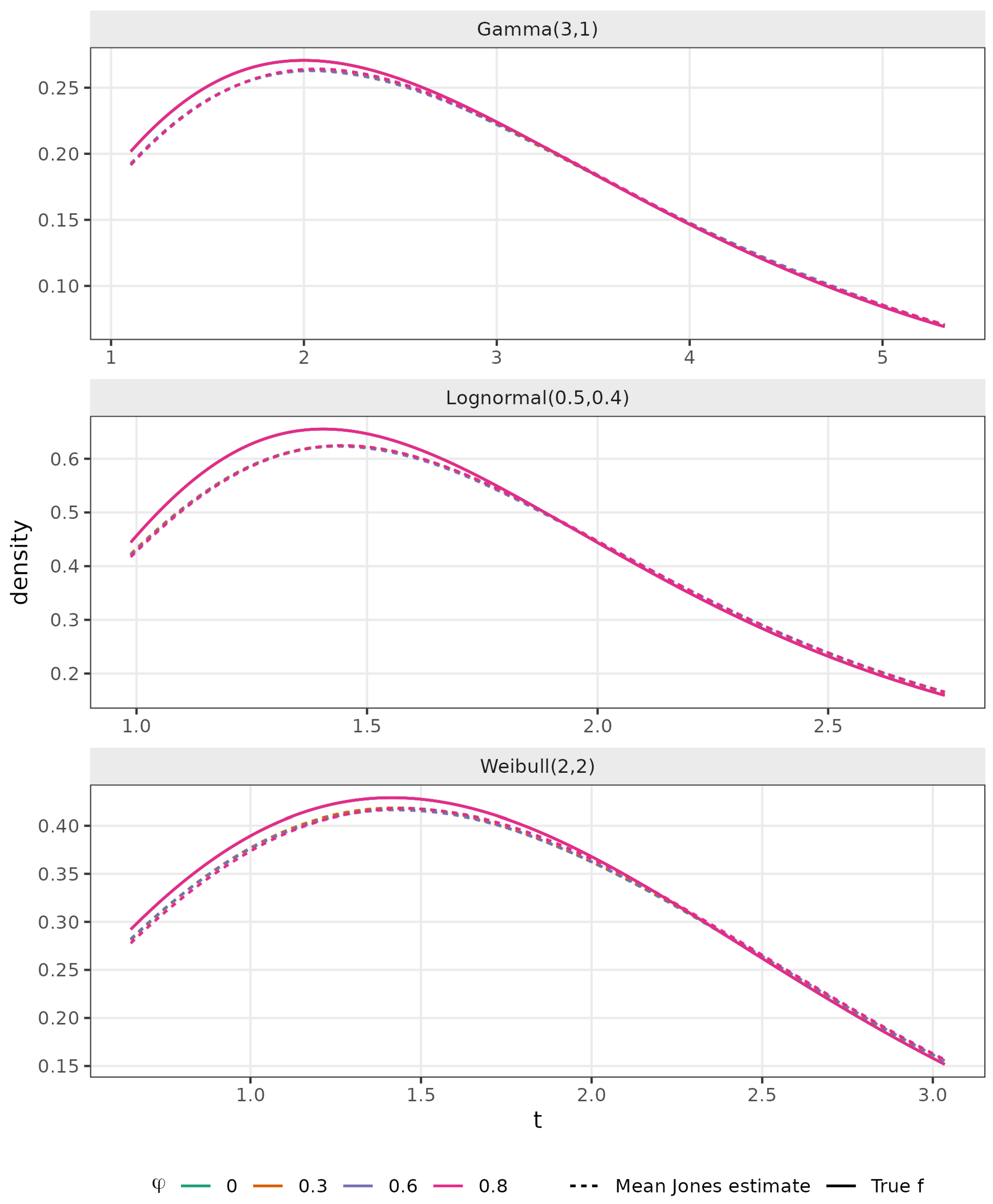
Figure 1 compares the Monte Carlo mean density estimate with the target density at $n=2000$. The principal shape of each target density is recovered under all four dependence levels. The more consequential effect of increasing dependence is not a systematic failure of density recovery but an increase in stochastic variability, which is quantified below.

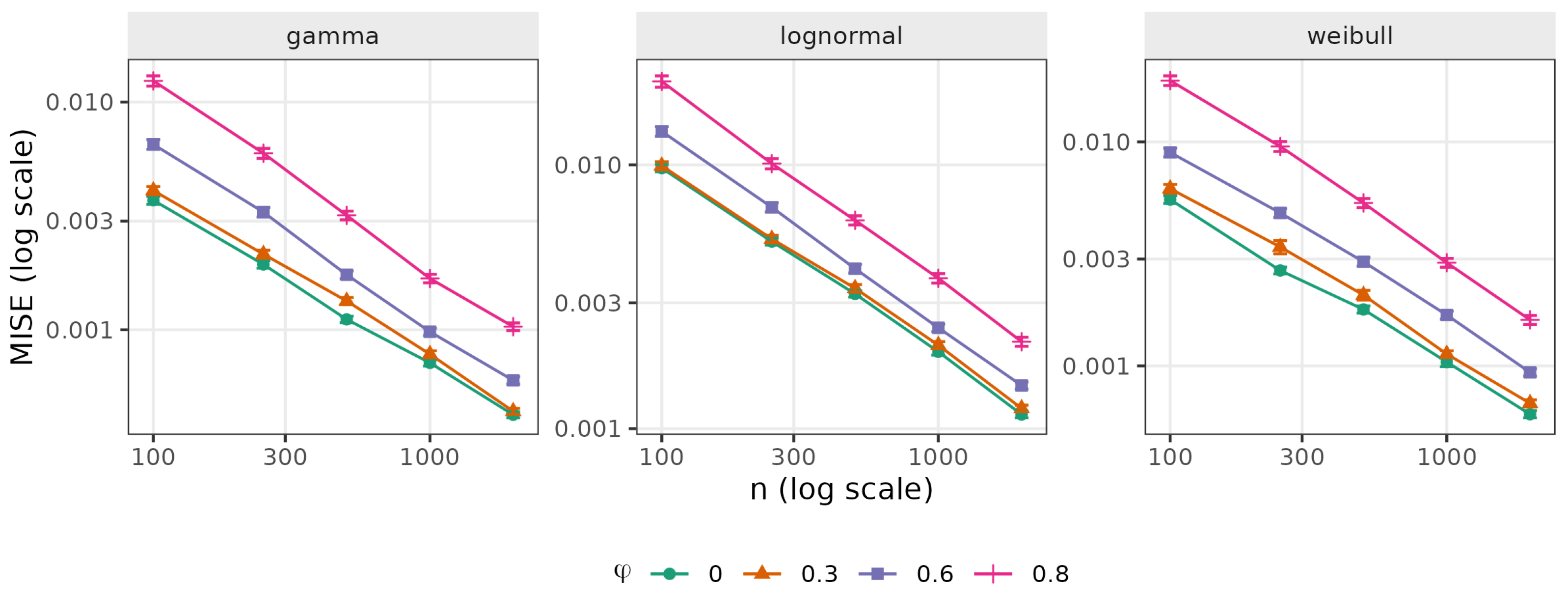
Figure 2 displays MISE against n on log–log axes, together with error bars of $\pm 2\mathrm{MCSE}\left\{\widehat{\mathrm{MISE}}\right\}$. Under independence, the OLS slope of $\log \left(\mathrm{MISE}\right)$ on $\log \left(n\right)$, using $n\in \{500,1000,2000\}$, is $-0.765$ for Gamma, $-0.714$ for Lognormal, and $-0.753$ for Weibull. At $\varphi =0.8$, the corresponding slopes are $-0.834$, $-0.831$, and $-0.897$.

These finite-range slopes are close to the first-order AMISE benchmark $-4/5$, but they are not interpreted as estimates of an asymptotic convergence exponent. The apparent steepening under stronger dependence can reflect the changing numerical importance of the serial covariance over the sample-size range considered. We therefore do not use these fitted slopes to claim a dependence-specific asymptotic rate.

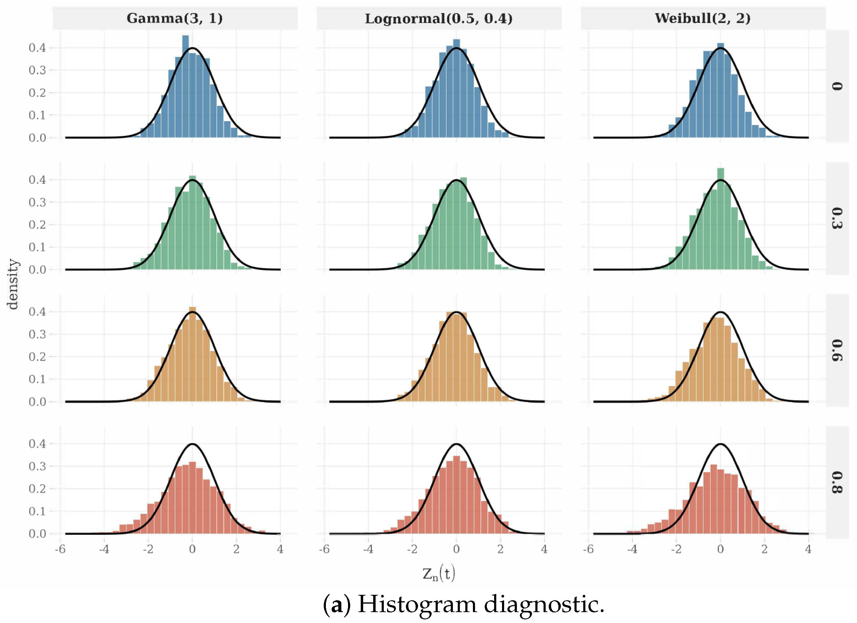
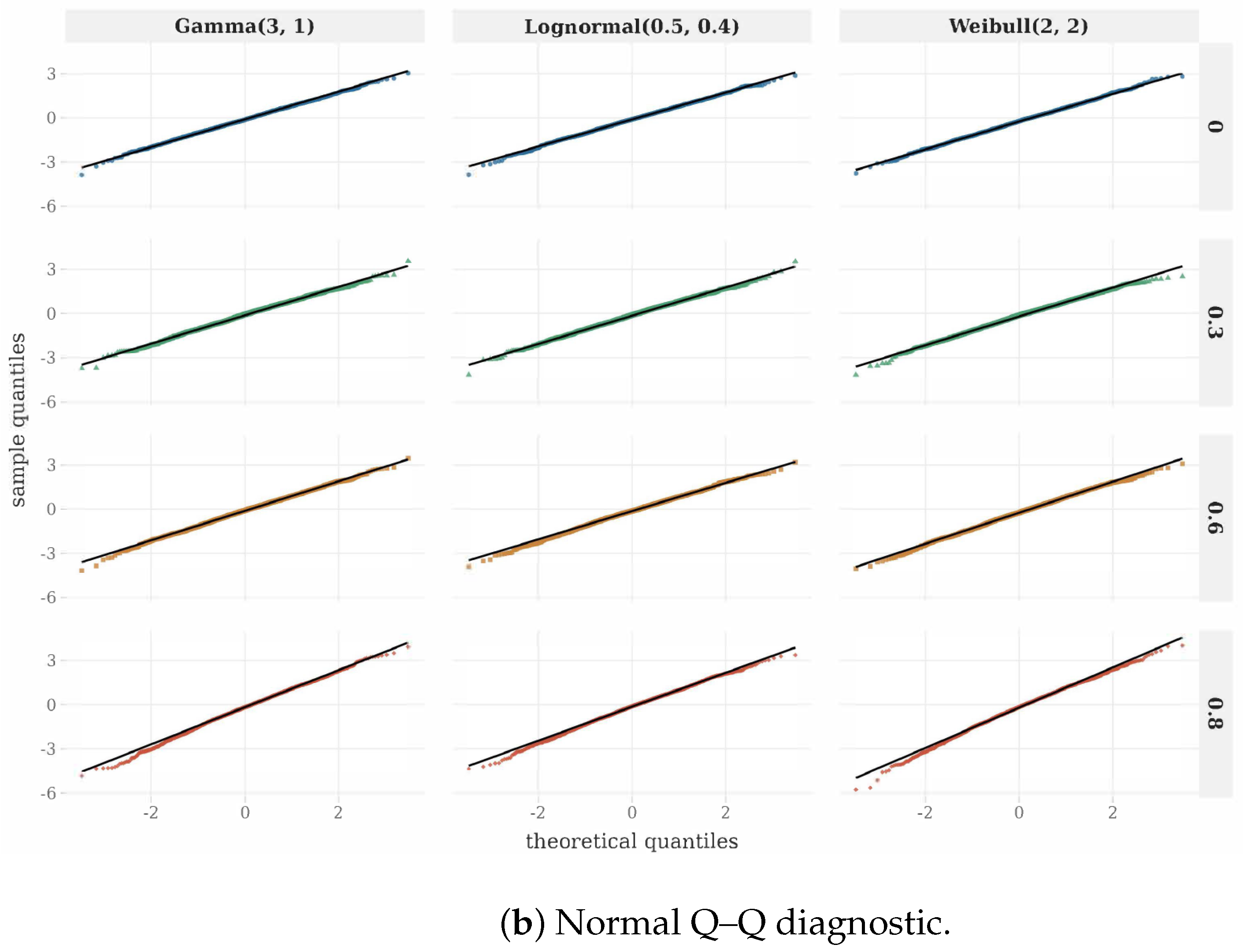
Figure 3 examines the Gaussian approximation for the studentized statistic at $q_{.50}$ when $n=2000$. Under independence and mild dependence, the distribution is comparatively close to standard normal. Under $\varphi =0.6$, and more clearly under $\varphi =0.8$, residual variance inflation, heavier tails, and asymmetry remain visible. The empirical Q–Q points are plotted explicitly so that departures in both the center and the tails can be assessed directly. These plots are finite-sample diagnostics of the Gaussian approximation, not graphical proofs of asymptotic normality.

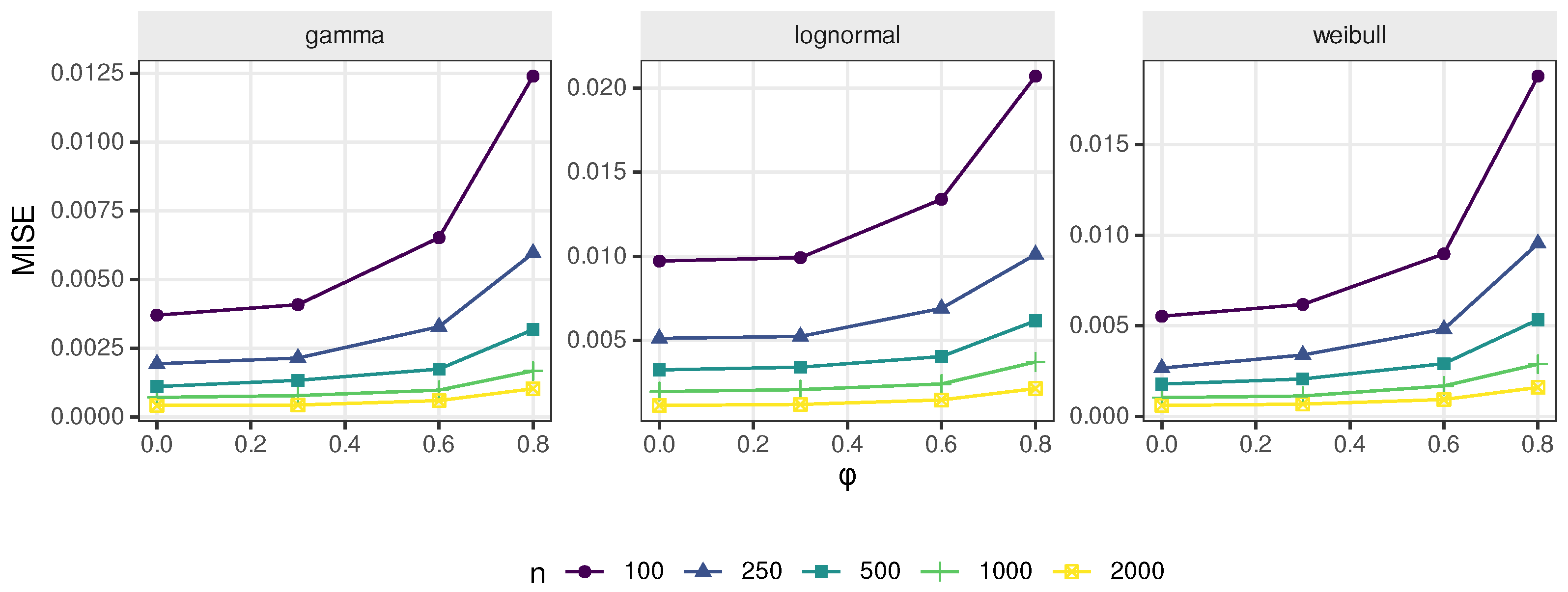
Figure 4 displays MISE directly as a function of $\varphi$. For every model and every simulated sample size, MISE increases as the dependence parameter increases, and the effect remains visible at $n=2000$. This is a finite-sample statement only. It is not extrapolated into a claim that the relative effect of dependence remains non-vanishing asymptotically.

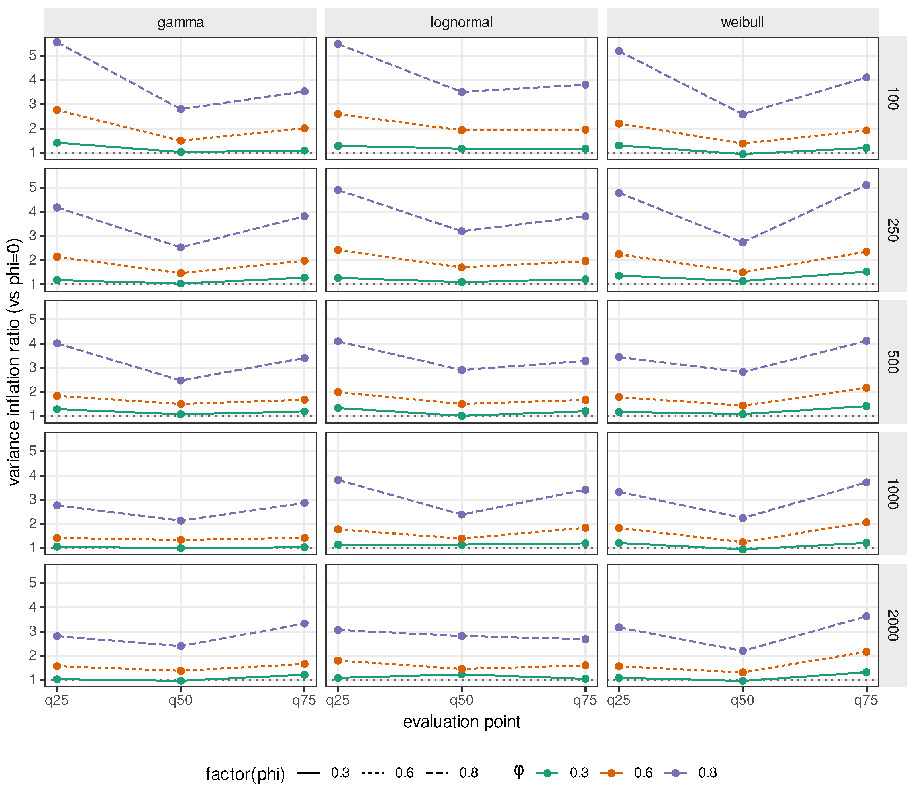
The variance-inflation ratio provides a more direct measure of the finite-sample dependence effect:

$$\mathrm{VIR}(\mathrm{model},n,\varphi ,t)={\displaystyle \frac{{\widehat{\mathrm{Var}}}_{\mathrm{MC},\varphi }\left\{f_n\left(t\right)\right\}}{{\widehat{\mathrm{Var}}}_{\mathrm{MC},0}\left\{f_n\left(t\right)\right\}}}.$$

At $n=2000$ and the grid point nearest $q_{.50}$, the variance under $\varphi =0.8$, relative to independence at the same sample size and oracle bandwidth, is inflated by factors $2.464$ for Gamma, $2.004$ for Lognormal, and $2.645$ for Weibull.

These are descriptive finite-sample variance ratios. They are not estimates of a non-zero asymptotic long-run variance multiplier. Their importance is interpretative: they show why the statement that the serial covariance is first-order negligible must not be paraphrased as saying that dependence has no finite-sample effect, see Figure 5.

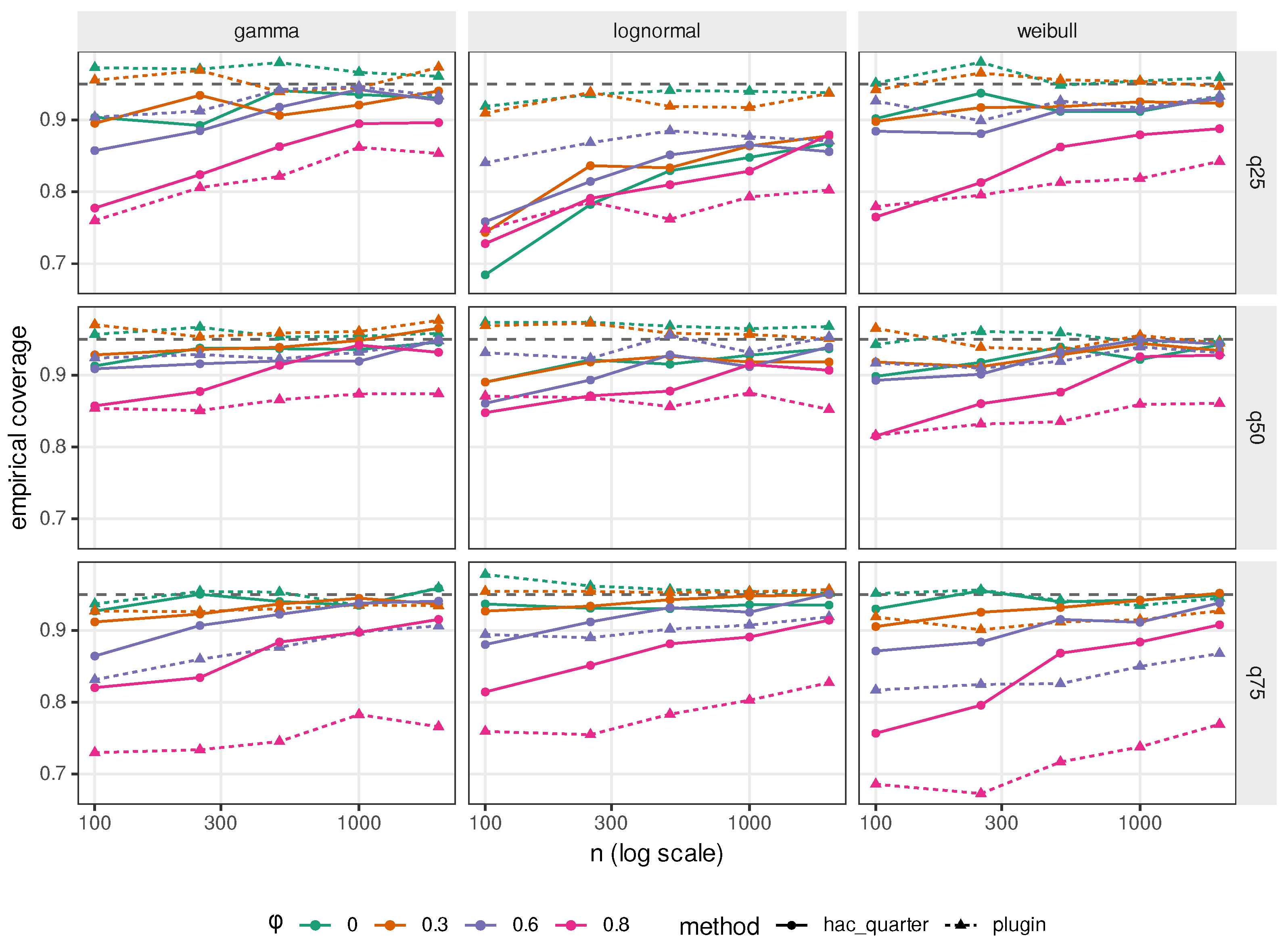
The coverage results provide the clearest finite-sample qualification of the first-order inference theory. Averaging over models, sample sizes, and evaluation points, empirical coverage is $0.961$ under independence and $0.948$ under mild dependence $(\varphi =0.3)$. Under moderate dependence $(\varphi =0.6)$, average coverage falls to $0.909$, while under $\varphi =0.8$ the corresponding average is $0.811$.

The same pattern remains evident at the largest sample size. At $n=2000$ and $\varphi =0.8$, average coverage over the three evaluation points is $0.831$ for Gamma, $0.866$ for Lognormal, and $0.818$ for Weibull. The upper-quartile point is often the most difficult; at $n=2000$ and $\varphi =0.8$, coverage at $q_{.75}$ is $0.782$ for Gamma and $0.765$ for Weibull.

Accordingly, we do not state that the intervals “approach the nominal coverage level” uniformly over the dependence regimes considered. Such a description is broadly supported over the simulated range under independence and mild dependence but not under $\varphi =0.6$ and, especially, not under $\varphi =0.8$.

This undercoverage does not contradict Theorem 3. The theorem identifies the first-order limiting variance for each fixed dependence parameter satisfying the stated conditions; it does not supply a finite-n rate for the coverage error. At finite n, the exact variance still contains the lagged covariance sum in (22), whereas the first-order plug-in variance estimator does not estimate that full finite-sample covariance component. The observed undercoverage under stronger dependence should therefore be viewed as a genuine limitation of first-order plug-in inference in this setting, rather than as a negligible numerical irregularity, see Figure 6.

4.7. Interpretation of the Numerical Results

Three conclusions emerge consistently from the simulation.

First, the estimator behaves in the manner suggested by the first-order estimation theory. Pointwise bias under $h_{\mathrm{AMISE}}$ decreases with n, MISE decreases systematically with sample size, and the empirical bias of ${\widehat{\mu }}_n$ is small in the reported scenarios, while its dispersion contracts as n increases. These findings are compatible with the second-order bias expansion and with the $O_{\mathbb{P}}\left(n^{-1/2}\right)$ stochastic order established for the random normalization.

Second, short-range dependence can remain materially important at finite sample sizes even though its contribution disappears from the first-order limiting variance. The monotone deterioration of MISE and the variance inflation ratios make this distinction especially clear. The mathematically correct interpretation is therefore not that dependence is “irrelevant” but that its serial covariance contribution is asymptotically of smaller order after the localization and normalization governing the kernel estimator.

Third, the finite-sample distribution of the studentized statistic deteriorates systematically as persistence increases. Table 16 shows pronounced left-skewness and heavy tails at small n under $\varphi =0.8$. For example, at $n=100$, the Gamma statistic at $q_{.25}$ has skewness $-2.067$ and excess kurtosis $13.212$. These distortions moderate as n grows, but they do not disappear uniformly over the simulated designs. Even at $n=2000$ and $\varphi =0.8$, the reported empirical variances of the studentized statistics range from $1.413$ to $2.732$, while all corresponding skewness coefficients remain negative, approximately between $-0.147$ and $-0.308$. This residual variance inflation and asymmetry provide a direct numerical explanation for the persistent undercoverage of the first-order normal plug-in interval.

Taken together, the Monte Carlo evidence supports the asymptotic results while also identifying their finite-sample boundary. Under geometric short-range dependence, the serial covariance disappears from the first-order limiting variance; nevertheless, stronger persistence can still produce substantial variance inflation, non-Gaussian studentized distributions, and meaningful undercoverage at sample sizes as large as $n=2000$. In applications where such dependence is plausible, first-order plug-in studentization should therefore be interpreted with appropriate caution. Dependence-adaptive finite-sample variance correction, higher-order studentization, and simultaneous confidence procedures are beyond the scope of the present paper and provide natural directions for further work.

4.8. Extended Computational Design and Reproducibility

The additional finite-sample experiments are organized as separate designs rather than pooled into a single simulation label. The primary Gaussian-copula AR(1) experiment contains 60 model–sample-size–dependence cells with $B=2000$ replications per cell. The Frank-copula Markov robustness experiment uses $B=2000$ for each of 18 cells. The feasible-bandwidth experiment uses $B=60$ per primary model cell and $B=30$ for the additional Gamma-mixture shape-sensitivity design; the estimator benchmark uses $B=200$; and the dependent-resampling experiment uses $B_{\mathrm{outer}}=100$ Monte Carlo samples with $B_{\mathrm{boot}}=200$ block resamples within each sample. The separation of these replication counts reflects their very different computational costs and prevents nested experiments from being confused with the primary Monte Carlo design, see

Table 4. Computational experiments and replication counts. The primary, robustness, bandwidth, benchmark, and nested resampling designs are reported separately.

Experiment	Replication Count	Role
Design A: Gaussian-copula AR(1)	60 cells, $B=2000$	Primary estimation and inference design.
Design B: Frank-copula Markov	18 cells, $B=2000$	Dependence robustness experiment.
Feasible bandwidth selectors	$B=60$; Gamma-mixture $B=30$	Feasible-selector comparison.
Estimator benchmark	$B=200$	Jones versus Bhattacharyya-type estimator on identical samples.
Dependent resampling	$B_{\mathrm{outer}}=100$, $B_{\mathrm{boot}}=200$	Dependent-resampling validation of finite-sample inference.

.

The computational pipeline uses master seed 20240517 together with deterministic cell- and replication-level seeds. The definitive run was executed under R 4.3.3 on x86_64-pc-linux-gnu (Ubuntu 24.04.4 LTS). The recorded workflow includes the RNG configuration, package versions, per-file SHA-256 hashes, and a combined source hash. Numerical tables and figures are generated from the same checkpointed machine-readable objects, so the graphical and tabular summaries cannot diverge through manual transcription.

4.9. Feasible Bandwidth Selection for the Jones Estimator

The oracle bandwidth $h_{\mathrm{AMISE}}$ isolates estimator behavior from bandwidth estimation error, but its constant depends on unknown features of f and is not available in applications. We therefore compare it with five feasible rules: a BGM-RT-style normal-reference selector, weighted cross-validation (WCV-Jones), SBoot1-Jones, SBoot2-Jones, and a contiguous leave-one-block-out cross-validation rule (Block-CV Jones). Every feasible bandwidth is recomputed from each replicated sample. Their empirical performance is evaluated directly; no asymptotic consistency or optimality property is inferred from the simulation.

The BGM-labeled procedures in the computational archive are independent, fully disclosed implementations of the corresponding published ideas rather than literal calls to the WData package. The terminology is therefore kept explicit—“BGM-RT-style”, “WCV-Jones”, “SBoot1-Jones”, and “SBoot2-Jones”—and the comparison estimator below is described as “Bhattacharyya-type”. This distinction concerns software provenance and does not alter the statistical definitions used in the numerical comparisons.

Table 5. Feasible bandwidth selection relative to the oracle AMISE bandwidth. The ratio range is computed after averaging the replication-level mean ratio over the three primary models within each $(n,\varphi )$ cell then taking the range across $n\in \{100,500,1000\}$ and $\varphi \in \{0,0.6\}$. Boundary frequencies are reported on the same aggregated grid.

Method	Range of $\overline{\mathit{h}}/{\mathit{h}}_{\mathbf{oracle}}$	Boundary Frequency	Failure Frequency
BGM-RT-style	0.936–0.984	not applicable	0.000
WCV-Jones	0.892–1.077	0.056–0.122	0.000
Block-CV Jones	0.905–1.108	0.044–0.144	0.000
SBoot1-Jones	1.612–1.823	0.000–0.000	0.000
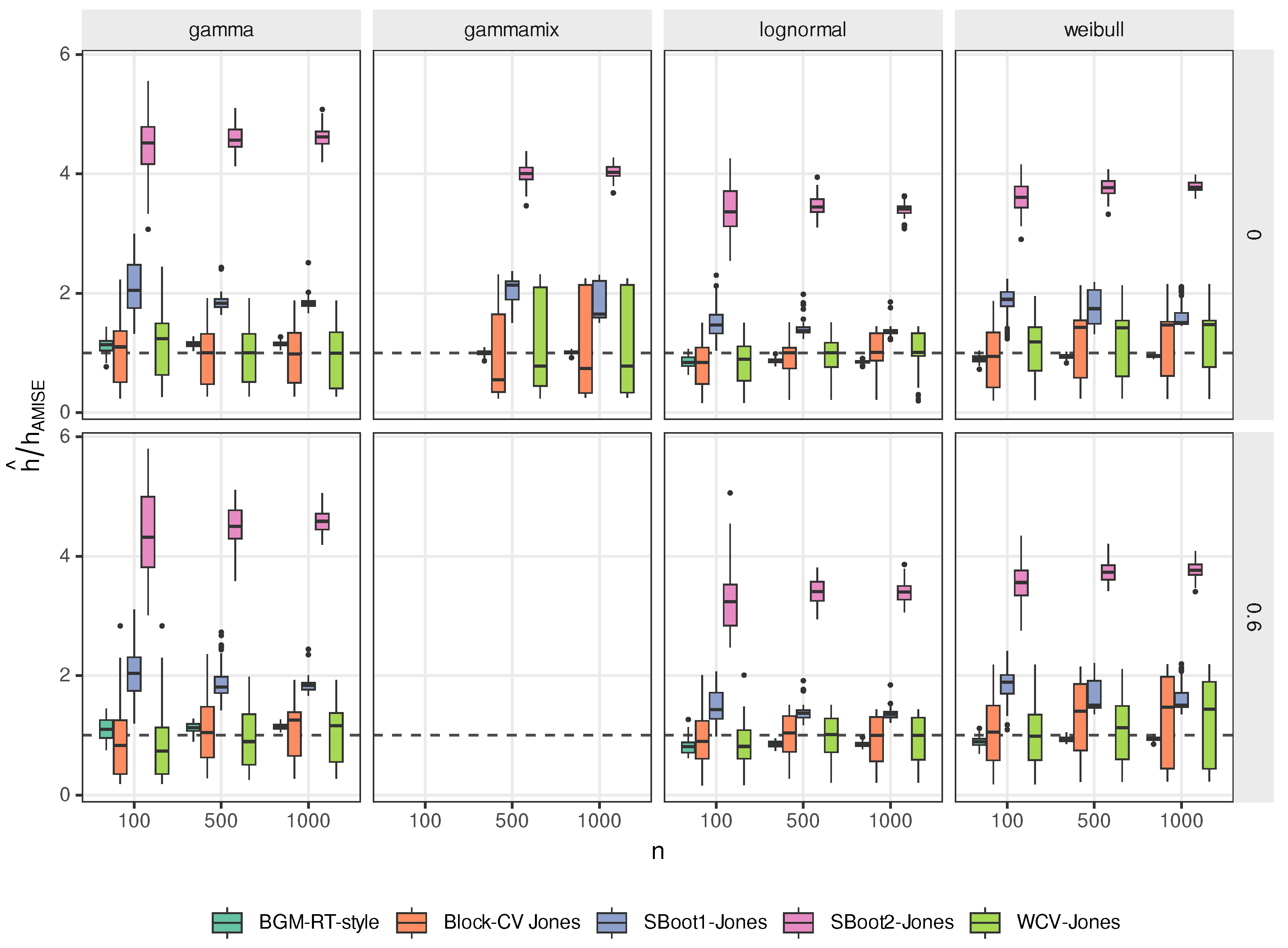
SBoot2-Jones	3.713–3.937	0.978–1.000	0.000

and Figure 7 summarize the model-averaged selected-to-oracle bandwidth ratios over $n\in \{100,500,1000\}$ and $\varphi \in \{0,0.6\}$ for the three primary models. WCV-Jones and Block-CV remain comparatively close to the oracle benchmark, whereas SBoot1 systematically selects larger bandwidths and SBoot2 is diagnostically unstable over the chosen search range: its upper boundary is selected in approximately $97.8$–$100\%$ of the aggregated cells. The additional Gamma-mixture experiment preserves the same ranking, with selected-to-oracle ranges 0.999–1.006 (BGM-RT-style), 1.144–1.155 (WCV-Jones), 0.987–1.133 (Block-CV), 1.869–2.025 (SBoot1), and 3.998–4.025 (SBoot2). Boundary solutions are reported rather than removed or winsorized.

The selector comparison addresses implementation, not the unresolved random-bandwidth asymptotics. Replacing a deterministic $h_n$ by a data-dependent ${\widehat{h}}_n$ in the dependent ratio estimator would require stochastic equicontinuity uniformly over a random bandwidth neighborhood, together with control of the selection criterion and the normalizer on the same probability space. Establishing such a result would constitute a distinct theoretical problem rather than a formal corollary of the oracle AMISE calculation.

4.10. Dependence-Robust Finite-Sample Inference

The principal finite-sample weakness of the first-order theory arises in studentization under strong persistence rather than in recovery of the density shape. We retain the plug-in interval as the asymptotic reference and examine two finite-sample corrections. For the HAC construction, write $a_i\left(t\right)=Y_i^{-1}{K}_h(t-Y_i)$, $b_i=Y_i^{-1}$, $A_n=\overline{a}$, $H_n=\overline{b}$, ${\widehat{\mu }}_n=H_n^{-1}$, and $f_n=A_n/H_n$. The empirical influence sequence is

$${\widehat{\psi }}_i\left(t\right)={\widehat{\mu }}_n\{a_i\left(t\right)-A_n\left(t\right)\}-{\widehat{\mu }}_n{f}_n\left(t\right)\{b_i-H_n\}.$$

A Bartlett/Newey–West estimator is formed from ${\widehat{\psi }}_i\left(t\right)$ using lag orders $L\asymp n^{1/4}$ and $L\asymp n^{1/3}$. The normalization component is therefore retained in the finite-sample correction, in agreement with the complete ratio expansion proved in Proposition 1. The HAC procedure is evaluated numerically and is not assigned an additional asymptotic validity theorem in this article.

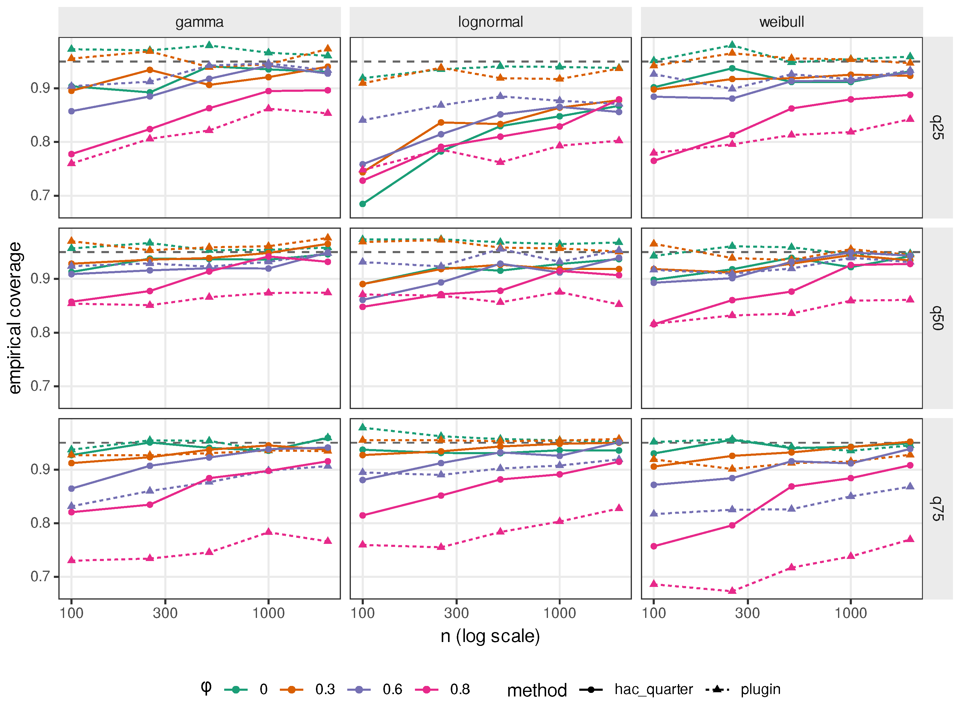
At the median point, averaging over the three primary models and $n\in \{1000,2000\}$, plug-in coverage equals 0.9566 under independence, 0.9394 at $\varphi =0.6$, and 0.8662 at $\varphi =0.8$. The quarter-order HAC values on the same cells are 0.9353, 0.9356, and 0.9250, while the third-order values are 0.9356, 0.9376, and 0.9334. The correction is consequently not uniformly preferable: when the plug-in interval is already well calibrated, it may widen the interval without improving coverage, whereas under strong persistence it recovers a substantial part of the coverage deficit.

At $n=2000$, $\varphi =0.8$, and $q_{.50}$, plug-in coverage is 0.8745, 0.8525, and 0.8610 for the Gamma, Lognormal, and Weibull targets. The quarter-order HAC rule raises these values to 0.9320, 0.9070, and 0.9280 and the third-order rule to 0.9405, 0.9180, and 0.9355, see

Table 6. Strong-dependence median-point inference at $n=2000$, $\varphi =0.8$ ($B=2000$). The last column is the ratio of mean interval length to the original plug-in interval.

Model	Method	Coverage	MCSE	Mean Length	Length Ratio
Gamma	Plug-in	0.8745	0.0074	0.05072	1.000
Gamma	HAC, $L\asymp n^{1/4}$	0.9320	0.0056	0.05903	1.164
Gamma	HAC, $L\asymp n^{1/3}$	0.9405	0.0053	0.06104	1.203
Lognormal	Plug-in	0.8525	0.0079	0.10416	1.000
Lognormal	HAC, $L\asymp n^{1/4}$	0.9070	0.0065	0.11513	1.105
Lognormal	HAC, $L\asymp n^{1/3}$	0.9180	0.0061	0.11959	1.148
Weibull	Plug-in	0.8610	0.0077	0.07715	1.000
Weibull	HAC, $L\asymp n^{1/4}$	0.9280	0.0058	0.09490	1.230
Weibull	HAC, $L\asymp n^{1/3}$	0.9355	0.0055	0.09866	1.279

. The corresponding mean interval-length ratios are 1.164, 1.105, and 1.230 for the quarter-order rule and 1.203, 1.148, and 1.279 for the third-order rule. Averaged over all three evaluation points at the same n and $\varphi$, the plug-in/quarter-order HAC coverages are 0.831/0.915 (Gamma), 0.828/0.900 (Lognormal), and 0.824/0.908 (Weibull). Thus, dependence-aware studentization materially improves the difficult cells, but it does not remove all coverage error.

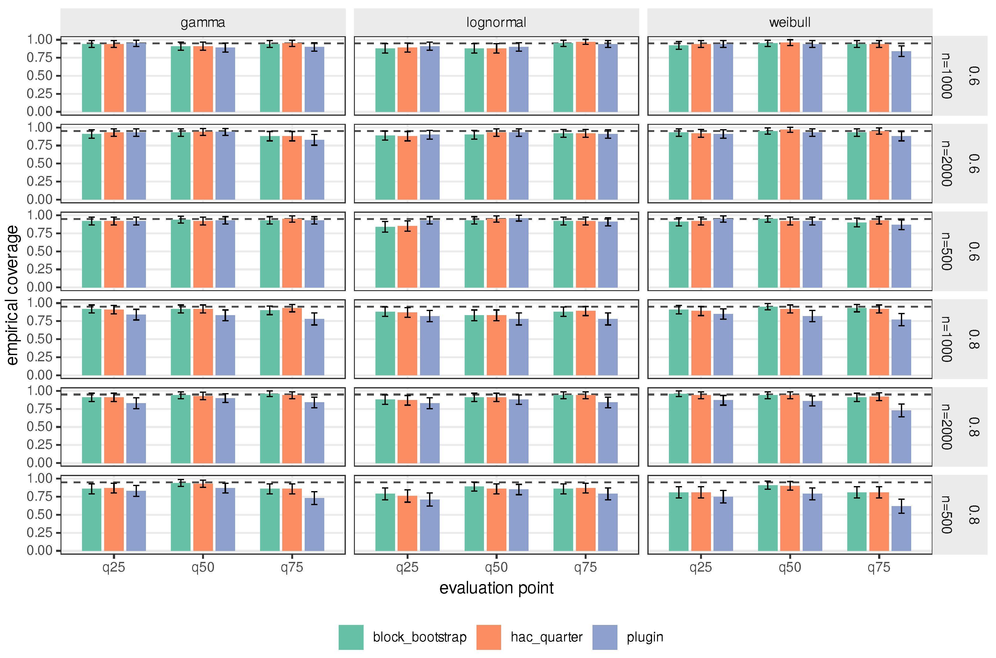
The moving-block-bootstrap experiment provides an independent resampling check on a designated high-persistence subset, see Figure 8. It uses $B_{\mathrm{outer}}=100$ Monte Carlo samples and $B_{\mathrm{boot}}=200$ block resamples per sample. At $n=1000$, $\varphi =0.8$, and $q_{.50}$, the Lognormal cell has coverage 0.78 for the plug-in interval and 0.83 for both HAC and the block bootstrap, see Figure 9. Because the outer experiment contains only 100 replications, its binomial Monte Carlo errors are necessarily larger than those of the primary design. The relevant conclusion is qualitative but important: dependence-aware corrections improve calibration in most difficult cells, yet no method examined here uniformly restores nominal coverage, see

Table 7. Dependent-resampling validation at $q_{.50}$ and $\varphi =0.8$ (outer $B=100$, inner block-bootstrap $B=200$). The last column gives the mean block-bootstrap to plug-in interval-length ratio.

n	Model	Plug-In	HAC	Block Bootstrap	Length Ratio
1000	Gamma	0.83	0.92	0.92	1.200
1000	Lognormal	0.78	0.83	0.83	1.105
1000	Weibull	0.82	0.92	0.95	1.241
2000	Gamma	0.90	0.93	0.94	1.168
2000	Lognormal	0.88	0.91	0.91	1.113
2000	Weibull	0.86	0.94	0.94	1.264

.

4.11. Robustness to a Second Dependence Mechanism

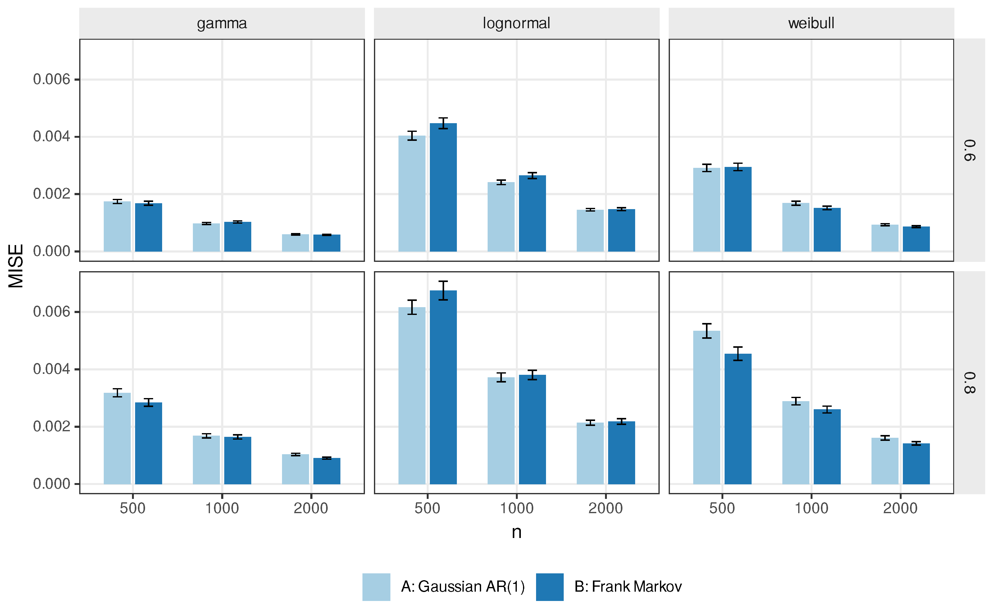
A second dependence design tests whether the preceding finite-sample pattern is specific to the Gaussian-copula AR(1) construction. Design B is a first-order Frank-copula Markov chain with uniform stationary marginal, transformed through the exact length-biased quantile function. Its Frank parameter is calibrated to the Gaussian design through Kendall’s $\tau =(2/\pi )\arcsin \left(\varphi \right)$. The values $\varphi =0.6$ and $0.8$ correspond to target Kendall coefficients 0.4097 and 0.5903 and Frank parameters 4.296 and 7.677, respectively. The marginal length-biased law is preserved by construction. This design is used as a robustness experiment; no claim is made that it constitutes an additional verified instance of every mixing assumption in the main theorems without a separate proof.

At $n=2000$, moving from the moderate to the stronger matched-dependence level increases MISE from 0.000583 to 0.000901 for Gamma, from 0.001476 to 0.002178 for Lognormal, and from 0.000870 to 0.001417 for Weibull. At the stronger level, median-point plug-in coverage is 0.916, 0.883, and 0.865; the quarter-order HAC correction raises these values to 0.934, 0.909, and 0.926. The same qualitative risk and coverage ordering therefore persists under a different copula mechanism, see

Table 8. Frank-copula Markov robustness design at $n=2000$ ($B=2000$). $\varphi$ indexes the Gaussian-AR(1) benchmark used only to define the matched Kendall $\tau$; $\theta$ is the corresponding Frank parameter. Coverage is reported at $q_{.50}$.

$\mathit{\varphi }$	Model	$\mathit{\theta }$	$\mathit{\tau }$	Lag-1	MISE	MCSE	Plug-In	HAC
0.6	Gamma	4.296	0.410	0.529	0.000583	0.000010	0.952	0.946
0.6	Lognormal	4.296	0.410	0.511	0.001476	0.000026	0.957	0.944
0.6	Weibull	4.296	0.410	0.554	0.000870	0.000015	0.958	0.953
0.8	Gamma	7.677	0.590	0.724	0.000901	0.000018	0.916	0.934
0.8	Lognormal	7.677	0.590	0.701	0.002178	0.000049	0.883	0.909
0.8	Weibull	7.677	0.590	0.751	0.001417	0.000030	0.865	0.926

and Figure 10.

4.12. Estimator Benchmark

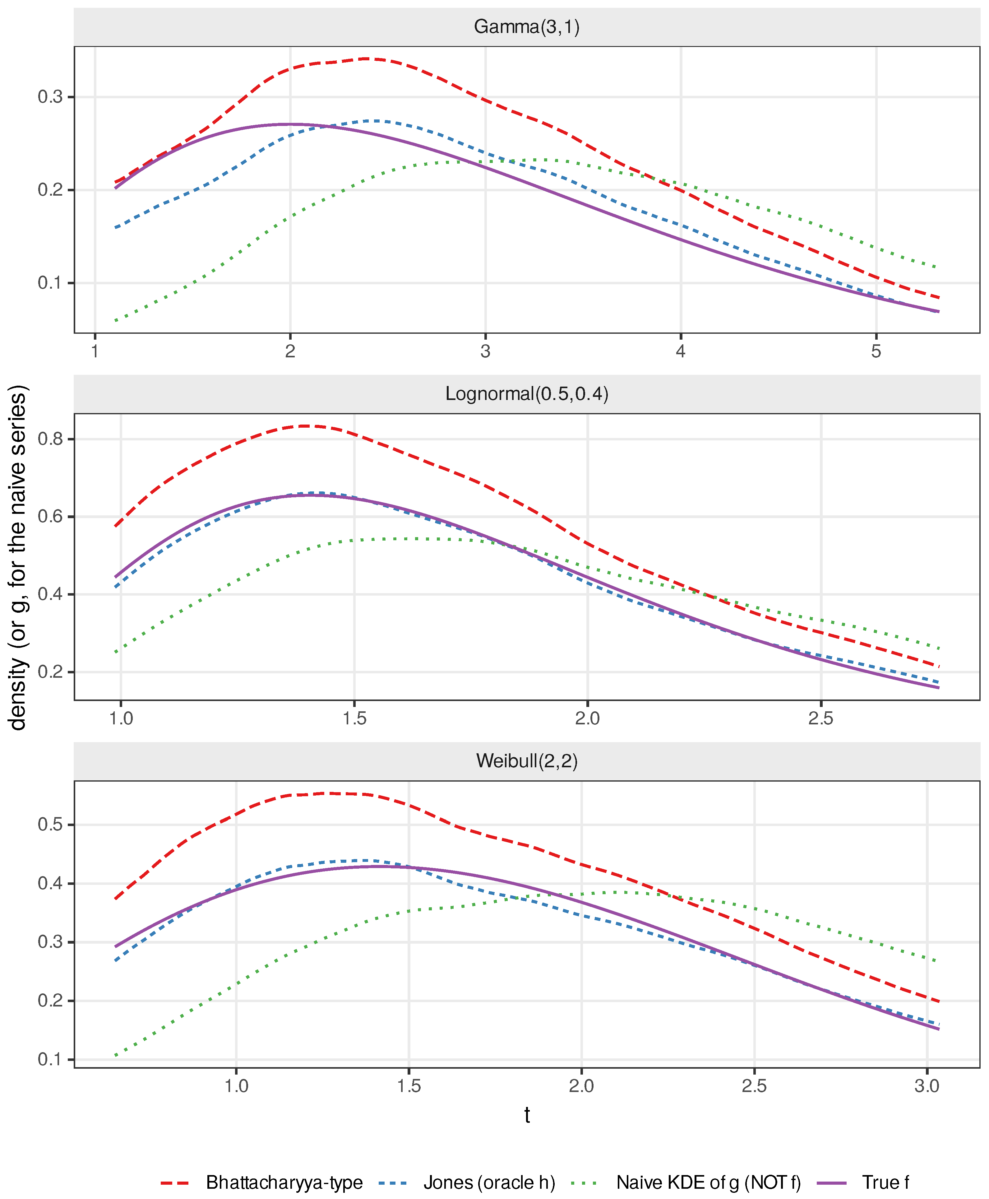
A separate $B=200$ experiment compares the Jones estimator under the oracle, WCV-Jones, and Block-CV bandwidths with an independently implemented Bhattacharyya-type smooth-then-divide estimator. An ordinary KDE of the observed $Y_i$’s is retained only as a negative control for the biased marginal g and is never interpreted as an estimator of the target density f.

At $n=2000$ under independence, the WCV/Block-CV Jones MISEs are 0.000868/0.000865 for Gamma, 0.002334/0.002229 for Lognormal, and 0.001539/0.001558 for Weibull, compared with 0.010941, 0.025066, and 0.018411 for the Bhattacharyya-type estimator, see

Table 9. MISE benchmark at $n=2000$ ($B=200$). “Bhattacharyya-type” denotes the independently coded smooth-then-divide implementation used in the computational workflow.

$\mathit{\varphi }$	Model	Jones Oracle	Jones WCV	Jones Block-CV	Bhattacharyya-Type
0.0	Gamma	0.000451	0.000868	0.000865	0.010941
0.0	Lognormal	0.001157	0.002334	0.002229	0.025066
0.0	Weibull	0.000594	0.001539	0.001558	0.018411
0.6	Gamma	0.000552	0.001096	0.001116	0.011150
0.6	Lognormal	0.001407	0.002591	0.002695	0.025512
0.6	Weibull	0.000806	0.001806	0.001956	0.018620

and Figure 11. The corresponding MISE advantage of the feasible Jones estimator is approximately 10.7–12.6-fold in these cells; at $\varphi =0.6$, the advantage is approximately 9.5–10.3-fold. These ratios are stated only for the reported $n=2000$ comparisons and are not extrapolated to smaller sample sizes.

4.13. Computational Validation

Fifteen automated validation checks were applied to the computational pipeline. They include the analytical Epanechnikov moments, exact length-biased samplers, marginal preservation under both dependence generators, normalization of the inverse-weighted empirical distribution, numerical integration of $f_n$, an independent numerical minimization of the oracle AMISE, bandwidth-selector finiteness and boundary diagnostics, the identity $\widehat{\mathrm{MSE}}={\widehat{\mathrm{Bias}}}^2+{\widehat{\mathrm{Var}}}_{\mathrm{MC}}$, the coverage-MCSE formula, HAC finiteness, block-bootstrap reconstruction, and deterministic seed reproducibility. All fifteen checks passed. Selected diagnostics are given in

Table 10. Selected diagnostics from the computational validation suite; all 15 prespecified checks passed.

Check	Definitive Diagnostic
Epanechnikov constants	$\int K=1$, $R\left(K\right)=0.600000$, $m_2\left(K\right)=0.200000$.
Exact length-biased sampler ($n=$ 200,000)	Maximum relative theoretical/empirical quantile discrepancy $=0.00329$.
Gaussian-AR(1) marginal check	KS $p\left(U\right)=p\left(Y\right)=0.2916$ at $\varphi =0.6$, $n=$ 20,000.
Frank-Markov marginal check	KS $p\left(U\right)=p\left(Y\right)=0.3634$, $\theta =4.2957$, $n=$ 20,000.
Inverse-weighted EDF	Total mass $=1.0000000000$.
Density integration	Wide-grid integral of a test $f_n=0.99874$.
Oracle AMISE validation	Maximum relative closed-form/numerical-minimizer discrepancy $2.82\times {10}^{-10}$ over four models.
HAC diagnostic	Bartlett LRV $=0.283187$, finite and non-negative in the validation cell.
Moving-block bootstrap	Length preserved (500) and identical under repeated fixed-seed execution.
Serial reproducibility	Identical ISE vectors under identical deterministic cell seeds.

.

During construction of the aggregate selector and benchmark summaries, two file-pattern collisions were detected by the validation workflow. The aggregation rules were corrected before the reported tables and figures were generated, and the entire validation suite was rerun successfully. The final numerical summaries are therefore taken only from the post-correction output objects.

4.14. Synthesis of the Numerical Evidence

The extended experiments sharpen, rather than replace, the interpretation of the asymptotic results. Feasible bandwidth selection is practically viable in the designs considered, but the quality of individual selectors differs substantially; WCV-Jones and Block-CV track the oracle much more closely than the two bootstrap rules over the reported search region. The full-ratio HAC correction materially improves coverage when serial persistence is strong, but it is not uniformly superior under weak dependence and does not eliminate every coverage defect. The moving-block experiment reaches the same qualitative conclusion. The Frank-copula Markov design reproduces the principal dependence pattern under a distinct copula mechanism. Finally, at $n=2000$, the feasible Jones estimator has substantially smaller MISE than the Bhattacharyya-type comparator in the tested cells. These are finite-sample statements. They neither modify the deterministic-bandwidth asymptotic theory nor imply new optimality, bootstrap, HAC, or Frank-process limit theorems.

4.15. Monte Carlo Tables

The following tables collect the numerical output from the primary $B=2000$ experiment: model-specific evaluation points, pointwise bias–variance–MSE summaries under the oracle bandwidth $h_{\mathrm{AMISE}}(I;n)$, MISE with Monte Carlo standard errors, empirical coverage of the studentized interval under the undersmoothing bandwidth $h_{\mathrm{US}}(I;n)$, normality moments of the studentized statistic $Z_n\left(t\right)$, and the behavior of ${\widehat{\mu }}_n$. MISE and pointwise bias/variance/MSE are reported under $h_{\mathrm{AMISE}}(I;n)$ only, and coverage and the studentized moments are reported under $h_{\mathrm{US}}(I;n)$ only, consistent with Section 4: the harmonic-mean estimator ${\widehat{\mu }}_n$ does not depend on the bandwidth and is therefore reported once per scenario.

Table 11. Model-specific evaluation points and true density values.

Model	${\mathit{q}}_{.25}$		${\mathit{q}}_{.50}$		${\mathit{q}}_{.75}$
	$\mathit{t}$	$\mathit{f}\left(\mathit{t}\right)$	$\mathit{t}$	$\mathit{f}\left(\mathit{t}\right)$	$\mathit{t}$	$\mathit{f}\left(\mathit{t}\right)$
Gamma	1.72730	0.26518	2.67406	0.24659	3.92040	0.15241
Lognormal	1.25886	0.63108	1.64872	0.60493	2.15933	0.36791
Weibull	1.07272	0.40227	1.66511	0.41628	2.35482	0.29435

The three points are the first quartile, median, and third quartile of the corresponding target distribution. These fixed values are not repeated in the pointwise performance tables.

,

Table 12. Pointwise bias, variance, and mean squared error under the oracle AMISE bandwidth.

n	$\mathit{\varphi }$	${\mathit{q}}_{.25}$			${\mathit{q}}_{.50}$			${\mathit{q}}_{.75}$
		Bias	Variance	MSE	Bias	Variance	MSE	Bias	Variance	MSE
Gamma
100	0	−0.02953	0.00080	0.00167	−0.00915	0.00077	0.00085	0.00426	0.00054	0.00056
100	0.3	−0.03007	0.00105	0.00196	−0.00977	0.00085	0.00094	0.00355	0.00067	0.00068
100	0.6	−0.03215	0.00182	0.00285	−0.00924	0.00108	0.00116	0.00528	0.00108	0.00111
100	0.8	−0.03636	0.00396	0.00528	−0.00762	0.00205	0.00211	0.00889	0.00197	0.00205
250	0	−0.02005	0.00046	0.00086	−0.00646	0.00040	0.00044	0.00248	0.00026	0.00026
250	0.3	−0.02069	0.00059	0.00102	−0.00582	0.00044	0.00047	0.00245	0.00031	0.00032
250	0.6	−0.02162	0.00090	0.00137	−0.00625	0.00062	0.00066	0.00292	0.00048	0.00049
250	0.8	−0.02398	0.00193	0.00251	−0.00538	0.00111	0.00114	0.00537	0.00088	0.00091
500	0	−0.01551	0.00031	0.00055	−0.00503	0.00026	0.00029	0.00176	0.00014	0.00014
500	0.3	−0.01571	0.00039	0.00063	−0.00519	0.00026	0.00029	0.00158	0.00017	0.00018
500	0.6	−0.01621	0.00053	0.00080	−0.00508	0.00036	0.00038	0.00213	0.00027	0.00028
500	0.8	−0.01740	0.00114	0.00144	−0.00487	0.00067	0.00070	0.00318	0.00051	0.00052
1000	0	−0.01153	0.00020	0.00033	−0.00408	0.00016	0.00018	0.00089	0.00009	0.00009
1000	0.3	−0.01192	0.00023	0.00037	−0.00340	0.00016	0.00017	0.00105	0.00010	0.00010
1000	0.6	−0.01125	0.00033	0.00046	−0.00361	0.00022	0.00023	0.00117	0.00015	0.00015
1000	0.8	−0.01302	0.00062	0.00079	−0.00316	0.00037	0.00038	0.00149	0.00027	0.00027
2000	0	−0.00910	0.00012	0.00020	−0.00261	0.00009	0.00009	0.00089	0.00005	0.00005
2000	0.3	−0.00877	0.00014	0.00022	−0.00292	0.00010	0.00011	0.00095	0.00006	0.00006
2000	0.6	−0.00891	0.00019	0.00027	−0.00278	0.00012	0.00013	0.00081	0.00008	0.00008
2000	0.8	−0.00975	0.00037	0.00047	−0.00373	0.00021	0.00023	0.00140	0.00015	0.00016
Lognormal
100	0	−0.06552	0.00381	0.00810	−0.02959	0.00384	0.00471	0.00749	0.00276	0.00281
100	0.3	−0.07085	0.00535	0.01037	−0.02991	0.00402	0.00491	0.01028	0.00337	0.00348
100	0.6	−0.07313	0.00906	0.01441	−0.02961	0.00560	0.00647	0.01319	0.00528	0.00545
100	0.8	−0.07853	0.01824	0.02441	−0.02740	0.01023	0.01098	0.01680	0.00945	0.00974
250	0	−0.04637	0.00224	0.00439	−0.01921	0.00204	0.00241	0.00507	0.00138	0.00141
250	0.3	−0.05026	0.00286	0.00539	−0.01825	0.00234	0.00267	0.00764	0.00168	0.00174
250	0.6	−0.05081	0.00430	0.00688	−0.02048	0.00294	0.00336	0.00766	0.00241	0.00247
250	0.8	−0.05446	0.00874	0.01170	−0.02031	0.00520	0.00562	0.00968	0.00444	0.00453
500	0	−0.03665	0.00141	0.00276	−0.01491	0.00126	0.00148	0.00360	0.00084	0.00085
500	0.3	−0.03551	0.00176	0.00302	−0.01518	0.00134	0.00157	0.00338	0.00095	0.00097
500	0.6	−0.03967	0.00263	0.00420	−0.01491	0.00182	0.00204	0.00569	0.00134	0.00137
500	0.8	−0.04092	0.00497	0.00665	−0.01296	0.00298	0.00315	0.00544	0.00240	0.00243
1000	0	−0.02887	0.00093	0.00176	−0.01043	0.00085	0.00096	0.00293	0.00043	0.00044
1000	0.3	−0.02723	0.00111	0.00186	−0.01174	0.00087	0.00101	0.00306	0.00057	0.00058
1000	0.6	−0.02859	0.00155	0.00237	−0.00966	0.00111	0.00121	0.00431	0.00078	0.00080
1000	0.8	−0.02925	0.00274	0.00359	−0.01103	0.00172	0.00185	0.00430	0.00133	0.00135
2000	0	−0.02210	0.00058	0.00107	−0.00759	0.00049	0.00055	0.00291	0.00029	0.00030
2000	0.3	−0.02078	0.00065	0.00108	−0.00874	0.00054	0.00062	0.00263	0.00032	0.00032
2000	0.6	−0.02331	0.00091	0.00146	−0.00826	0.00062	0.00069	0.00359	0.00042	0.00043
2000	0.8	−0.02311	0.00164	0.00217	−0.00870	0.00099	0.00106	0.00297	0.00070	0.00071
Weibull
100	0	−0.03769	0.00167	0.00309	−0.02520	0.00182	0.00246	−0.00266	0.00150	0.00151
100	0.3	−0.04091	0.00226	0.00394	−0.02633	0.00187	0.00256	0.00000	0.00194	0.00194
100	0.6	−0.04075	0.00411	0.00577	−0.02495	0.00286	0.00348	−0.00010	0.00332	0.00332
100	0.8	−0.04818	0.00809	0.01041	−0.02206	0.00475	0.00524	0.00811	0.00619	0.00626
250	0	−0.02672	0.00097	0.00168	−0.01871	0.00099	0.00134	−0.00130	0.00069	0.00069
250	0.3	−0.02749	0.00124	0.00200	−0.01815	0.00103	0.00136	−0.00142	0.00090	0.00091
250	0.6	−0.02902	0.00207	0.00291	−0.01816	0.00148	0.00181	0.00003	0.00155	0.00155
250	0.8	−0.03004	0.00422	0.00512	−0.01594	0.00287	0.00312	0.00248	0.00308	0.00309
500	0	−0.02073	0.00066	0.00109	−0.01313	0.00061	0.00078	−0.00061	0.00040	0.00040
500	0.3	−0.02167	0.00080	0.00127	−0.01376	0.00066	0.00085	−0.00050	0.00050	0.00050
500	0.6	−0.02179	0.00126	0.00174	−0.01375	0.00093	0.00112	−0.00059	0.00084	0.00084
500	0.8	−0.02297	0.00266	0.00318	−0.01112	0.00175	0.00188	0.00273	0.00186	0.00186
1000	0	−0.01567	0.00041	0.00065	−0.01067	0.00036	0.00047	−0.00126	0.00024	0.00024
1000	0.3	−0.01601	0.00050	0.00076	−0.01135	0.00038	0.00050	−0.00103	0.00028	0.00028
1000	0.6	−0.01602	0.00073	0.00099	−0.01119	0.00056	0.00068	−0.00078	0.00045	0.00045
1000	0.8	−0.01749	0.00141	0.00171	−0.01094	0.00096	0.00108	0.00110	0.00091	0.00091
2000	0	−0.01195	0.00025	0.00039	−0.00853	0.00021	0.00028	−0.00102	0.00014	0.00014
2000	0.3	−0.01172	0.00031	0.00045	−0.00807	0.00024	0.00030	−0.00098	0.00016	0.00016
2000	0.6	−0.01234	0.00043	0.00058	−0.00856	0.00030	0.00037	−0.00046	0.00025	0.00025
2000	0.8	−0.01297	0.00080	0.00097	−0.00773	0.00056	0.00062	−0.00018	0.00045	0.00045

Rows are grouped by model. The entries are Monte Carlo estimates ($B=2000$) at the three evaluation points reported in Table 11 under the oracle bandwidth $h_{\mathrm{AMISE}}(I;n)$. Variance uses the population (divide-by-B) convention, and $\mathrm{MSE}={\mathrm{Bias}}^2+\mathrm{Variance}$ was verified numerically for every row.

,

Table 13. Mean integrated squared error under the oracle AMISE bandwidth.

n	$\mathit{\varphi }$	MISE	$\mathrm{se}\left(\mathrm{MISE}\right)$
Gamma
100	0	0.003719	0.000073
100	0.3	0.004416	0.000095
100	0.6	0.006455	0.000155
100	0.8	0.012028	0.000299
250	0	0.001894	0.000034
250	0.3	0.002208	0.000044
250	0.6	0.003199	0.000067
250	0.8	0.005768	0.000131
500	0	0.001185	0.000020
500	0.3	0.001324	0.000024
500	0.6	0.001838	0.000037
500	0.8	0.003406	0.000079
1000	0	0.000709	0.000012
1000	0.3	0.000786	0.000013
1000	0.6	0.001052	0.000020
1000	0.8	0.001827	0.000037
2000	0	0.000411	0.000006
2000	0.3	0.000462	0.000007
2000	0.6	0.000590	0.000011
2000	0.8	0.001071	0.000022
Lognormal
100	0	0.007549	0.000145
100	0.3	0.009326	0.000191
100	0.6	0.013293	0.000313
100	0.8	0.023654	0.000554
250	0	0.003931	0.000071
250	0.3	0.004794	0.000089
250	0.6	0.006403	0.000133
250	0.8	0.011307	0.000252
500	0	0.002403	0.000040
500	0.3	0.002690	0.000049
500	0.6	0.003791	0.000073
500	0.8	0.006317	0.000140
1000	0	0.001489	0.000023
1000	0.3	0.001659	0.000027
1000	0.6	0.002202	0.000042
1000	0.8	0.003489	0.000072
2000	0	0.000894	0.000013
2000	0.3	0.000972	0.000015
2000	0.6	0.001279	0.000022
2000	0.8	0.001996	0.000039
Weibull
100	0	0.005142	0.000112
100	0.3	0.006371	0.000137
100	0.6	0.009763	0.000223
100	0.8	0.017345	0.000411
250	0	0.002690	0.000051
250	0.3	0.003167	0.000062
250	0.6	0.004864	0.000114
250	0.8	0.008897	0.000208
500	0	0.001644	0.000030
500	0.3	0.001912	0.000038
500	0.6	0.002817	0.000063
500	0.8	0.005443	0.000131
1000	0	0.000982	0.000017
1000	0.3	0.001128	0.000021
1000	0.6	0.001604	0.000031
1000	0.8	0.002892	0.000061
2000	0	0.000579	0.000009
2000	0.3	0.000663	0.000011
2000	0.6	0.000903	0.000016
2000	0.8	0.001570	0.000032

se(MISE) denotes the Monte Carlo standard error of the reported MISE, $\mathrm{sd}\left(\mathrm{ISE}\right)/\sqrt{B}$, $B=2000$. MISE is reported under the oracle AMISE bandwidth $h_{\mathrm{AMISE}}(I;n)$ only.

,

Table 14. Empirical coverage probabilities for nominal 95% studentized confidence intervals; Monte Carlo standard errors are shown in parentheses.

n	$\mathit{\varphi }$	${\mathit{q}}_{.25}$	${\mathit{q}}_{.50}$	${\mathit{q}}_{.75}$
Gamma
100	0	0.963 (0.004)	0.965 (0.004)	0.947 (0.005)
100	0.3	0.949 (0.005)	0.960 (0.004)	0.923 (0.006)
100	0.6	0.895 (0.007)	0.932 (0.006)	0.854 (0.008)
100	0.8	0.781 (0.009)	0.855 (0.008)	0.726 (0.010)
250	0	0.972 (0.004)	0.966 (0.004)	0.952 (0.005)
250	0.3	0.950 (0.005)	0.961 (0.004)	0.930 (0.006)
250	0.6	0.917 (0.006)	0.928 (0.006)	0.867 (0.008)
250	0.8	0.805 (0.009)	0.849 (0.008)	0.750 (0.010)
500	0	0.965 (0.004)	0.965 (0.004)	0.956 (0.005)
500	0.3	0.951 (0.005)	0.964 (0.004)	0.930 (0.006)
500	0.6	0.929 (0.006)	0.941 (0.005)	0.873 (0.007)
500	0.8	0.813 (0.009)	0.838 (0.008)	0.762 (0.010)
1000	0	0.967 (0.004)	0.960 (0.004)	0.945 (0.005)
1000	0.3	0.952 (0.005)	0.959 (0.004)	0.925 (0.006)
1000	0.6	0.935 (0.005)	0.941 (0.005)	0.885 (0.007)
1000	0.8	0.832 (0.008)	0.859 (0.008)	0.772 (0.009)
2000	0	0.964 (0.004)	0.966 (0.004)	0.951 (0.005)
2000	0.3	0.957 (0.005)	0.955 (0.005)	0.938 (0.005)
2000	0.6	0.926 (0.006)	0.949 (0.005)	0.908 (0.006)
2000	0.8	0.849 (0.008)	0.862 (0.008)	0.782 (0.009)
Lognormal
100	0	0.968 (0.004)	0.970 (0.004)	0.969 (0.004)
100	0.3	0.938 (0.005)	0.968 (0.004)	0.955 (0.005)
100	0.6	0.886 (0.007)	0.940 (0.005)	0.899 (0.007)
100	0.8	0.777 (0.009)	0.870 (0.008)	0.786 (0.009)
250	0	0.969 (0.004)	0.972 (0.004)	0.960 (0.004)
250	0.3	0.950 (0.005)	0.970 (0.004)	0.949 (0.005)
250	0.6	0.916 (0.006)	0.943 (0.005)	0.905 (0.007)
250	0.8	0.818 (0.009)	0.883 (0.007)	0.792 (0.009)
500	0	0.973 (0.004)	0.973 (0.004)	0.956 (0.005)
500	0.3	0.961 (0.004)	0.967 (0.004)	0.952 (0.005)
500	0.6	0.921 (0.006)	0.945 (0.005)	0.911 (0.006)
500	0.8	0.835 (0.008)	0.896 (0.007)	0.814 (0.009)
1000	0	0.961 (0.004)	0.963 (0.004)	0.968 (0.004)
1000	0.3	0.953 (0.005)	0.966 (0.004)	0.942 (0.005)
1000	0.6	0.935 (0.005)	0.946 (0.005)	0.912 (0.006)
1000	0.8	0.859 (0.008)	0.890 (0.007)	0.824 (0.009)
2000	0	0.964 (0.004)	0.963 (0.004)	0.959 (0.004)
2000	0.3	0.963 (0.004)	0.961 (0.004)	0.951 (0.005)
2000	0.6	0.929 (0.006)	0.946 (0.005)	0.920 (0.006)
2000	0.8	0.858 (0.008)	0.889 (0.007)	0.851 (0.008)
Weibull
100	0	0.967 (0.004)	0.950 (0.005)	0.937 (0.005)
100	0.3	0.952 (0.005)	0.946 (0.005)	0.911 (0.006)
100	0.6	0.901 (0.007)	0.904 (0.007)	0.804 (0.009)
100	0.8	0.776 (0.009)	0.844 (0.008)	0.676 (0.010)
250	0	0.970 (0.004)	0.955 (0.005)	0.949 (0.005)
250	0.3	0.963 (0.004)	0.946 (0.005)	0.911 (0.006)
250	0.6	0.907 (0.006)	0.903 (0.007)	0.835 (0.008)
250	0.8	0.791 (0.009)	0.814 (0.009)	0.685 (0.010)
500	0	0.964 (0.004)	0.953 (0.005)	0.951 (0.005)
500	0.3	0.951 (0.005)	0.948 (0.005)	0.930 (0.006)
500	0.6	0.911 (0.006)	0.921 (0.006)	0.848 (0.008)
500	0.8	0.790 (0.009)	0.828 (0.008)	0.679 (0.010)
1000	0	0.963 (0.004)	0.959 (0.004)	0.947 (0.005)
1000	0.3	0.956 (0.005)	0.952 (0.005)	0.924 (0.006)
1000	0.6	0.923 (0.006)	0.910 (0.006)	0.860 (0.008)
1000	0.8	0.826 (0.008)	0.827 (0.008)	0.727 (0.010)
2000	0	0.973 (0.004)	0.954 (0.005)	0.949 (0.005)
2000	0.3	0.956 (0.005)	0.949 (0.005)	0.927 (0.006)
2000	0.6	0.929 (0.006)	0.932 (0.006)	0.868 (0.008)
2000	0.8	0.843 (0.008)	0.846 (0.008)	0.765 (0.009)

Each entry is empirical coverage with its binomial Monte Carlo standard error in parentheses, ${\{\widehat{p}(1-\widehat{p})/2000\}}^{1/2}$. The nominal coverage level is 0.95 and all entries use the undersmoothing bandwidth $h_{\mathrm{US}}(I;n)$. Persistent undercoverage under stronger dependence is interpreted as a finite-sample limitation of first-order plug-in inference.

,

Table 15. Monte Carlo behavior of the estimated mean parameter ${\widehat{\mu }}_n$.

n	$\mathit{\varphi }$	$\mathit{\mu }$	Mean $\left({\widehat{\mathit{\mu }}}_{\mathit{n}}\right)$	SD $\left({\widehat{\mathit{\mu }}}_{\mathit{n}}\right)$
Gamma
100	0	3.0000	3.0157	0.2097
100	0.3	3.0000	3.0239	0.2700
100	0.6	3.0000	3.0382	0.3869
100	0.8	3.0000	3.1017	0.5534
250	0	3.0000	3.0025	0.1309
250	0.3	3.0000	3.0096	0.1708
250	0.6	3.0000	3.0173	0.2430
250	0.8	3.0000	3.0438	0.3540
500	0	3.0000	3.0056	0.0950
500	0.3	3.0000	3.0015	0.1228
500	0.6	3.0000	3.0115	0.1739
500	0.8	3.0000	3.0295	0.2635
1000	0	3.0000	2.9974	0.0677
1000	0.3	3.0000	3.0023	0.0864
1000	0.6	3.0000	3.0009	0.1232
1000	0.8	3.0000	3.0063	0.1812
2000	0	3.0000	3.0006	0.0466
2000	0.3	3.0000	3.0006	0.0627
2000	0.6	3.0000	3.0014	0.0877
2000	0.8	3.0000	3.0100	0.1303
Lognormal
100	0	1.7860	1.7880	0.0738
100	0.3	1.7860	1.7956	0.1014
100	0.6	1.7860	1.7986	0.1410
100	0.8	1.7860	1.8102	0.2142
250	0	1.7860	1.7869	0.0466
250	0.3	1.7860	1.7906	0.0633
250	0.6	1.7860	1.7945	0.0890
250	0.8	1.7860	1.7983	0.1350
500	0	1.7860	1.7855	0.0328
500	0.3	1.7860	1.7865	0.0438
500	0.6	1.7860	1.7899	0.0643
500	0.8	1.7860	1.7911	0.0961
1000	0	1.7860	1.7860	0.0235
1000	0.3	1.7860	1.7857	0.0316
1000	0.6	1.7860	1.7883	0.0460
1000	0.8	1.7860	1.7876	0.0673
2000	0	1.7860	1.7864	0.0168
2000	0.3	1.7860	1.7866	0.0225
2000	0.6	1.7860	1.7888	0.0322
2000	0.8	1.7860	1.7871	0.0486
Weibull
100	0	1.7725	1.7744	0.1288
100	0.3	1.7725	1.7898	0.1599
100	0.6	1.7725	1.7940	0.2237
100	0.8	1.7725	1.8226	0.3064
250	0	1.7725	1.7763	0.0822
250	0.3	1.7725	1.7769	0.1005
250	0.6	1.7725	1.7841	0.1464
250	0.8	1.7725	1.7922	0.2082
500	0	1.7725	1.7764	0.0582
500	0.3	1.7725	1.7765	0.0732
500	0.6	1.7725	1.7780	0.1011
500	0.8	1.7725	1.7896	0.1535
1000	0	1.7725	1.7734	0.0417
1000	0.3	1.7725	1.7733	0.0520
1000	0.6	1.7725	1.7722	0.0722
1000	0.8	1.7725	1.7813	0.1077
2000	0	1.7725	1.7720	0.0297
2000	0.3	1.7725	1.7723	0.0374
2000	0.6	1.7725	1.7728	0.0509
2000	0.8	1.7725	1.7767	0.0756

$\mu$ is the true mean of the target distribution; Mean$\left(\widehat{\mu }\right)$ and SD$\left(\widehat{\mu }\right)$ are computed over the $B=2000$ Monte Carlo replications. ${\widehat{\mu }}_n$ does not depend on the bandwidth and is computed once per replicated sample.

and

Table 16. Empirical moments of the studentized statistic $Z_n\left(t\right)$.

n	$\mathit{\varphi }$	Point	Mean	Variance	Skewness	Excess Kurtosis
Gamma
100	0	$q_{.25}$	−0.442	0.607	−0.511	0.584
100	0	$q_{.50}$	−0.206	0.768	−0.378	0.361
100	0	$q_{.75}$	0.029	1.007	−0.328	−0.031
100	0.3	$q_{.25}$	−0.467	0.741	−0.535	1.228
100	0.3	$q_{.50}$	−0.223	0.878	−0.503	0.645
100	0.3	$q_{.75}$	−0.034	1.275	−0.562	0.972
100	0.6	$q_{.25}$	−0.530	1.235	−0.817	1.374
100	0.6	$q_{.50}$	−0.226	1.104	−0.726	1.499
100	0.6	$q_{.75}$	−0.065	2.111	−0.834	1.600
100	0.8	$q_{.25}$	−0.750	3.530	−2.067	13.212
100	0.8	$q_{.50}$	−0.243	2.075	−0.864	1.438
100	0.8	$q_{.75}$	−0.095	3.888	−1.064	1.899
250	0	$q_{.25}$	−0.377	0.661	−0.365	0.610
250	0	$q_{.50}$	−0.170	0.792	−0.283	0.201
250	0	$q_{.75}$	0.033	0.987	−0.215	−0.024
250	0.3	$q_{.25}$	−0.397	0.776	−0.319	0.170
250	0.3	$q_{.50}$	−0.152	0.850	−0.334	0.317
250	0.3	$q_{.75}$	0.005	1.167	−0.223	0.046
250	0.6	$q_{.25}$	−0.440	1.089	−0.240	−0.008
250	0.6	$q_{.50}$	−0.186	1.150	−0.350	0.318
250	0.6	$q_{.75}$	−0.019	1.713	−0.315	0.123
250	0.8	$q_{.25}$	−0.565	2.348	−0.547	0.554
250	0.8	$q_{.50}$	−0.197	1.953	−0.416	0.142
250	0.8	$q_{.75}$	0.001	3.058	−0.603	0.752
500	0	$q_{.25}$	−0.336	0.704	−0.266	−0.045
500	0	$q_{.50}$	−0.166	0.836	−0.194	0.086
500	0	$q_{.75}$	0.024	0.956	−0.085	−0.125
500	0.3	$q_{.25}$	−0.356	0.819	−0.141	−0.085
500	0.3	$q_{.50}$	−0.172	0.865	−0.194	0.030
500	0.3	$q_{.75}$	0.001	1.152	−0.226	0.044
500	0.6	$q_{.25}$	−0.373	1.028	−0.253	0.305
500	0.6	$q_{.50}$	−0.175	1.081	−0.188	−0.103
500	0.6	$q_{.75}$	0.008	1.636	−0.221	−0.000
500	0.8	$q_{.25}$	−0.454	2.084	−0.408	0.326
500	0.8	$q_{.50}$	−0.224	1.956	−0.421	0.739
500	0.8	$q_{.75}$	−0.009	3.015	−0.557	0.988
1000	0	$q_{.25}$	−0.297	0.764	−0.286	0.255
1000	0	$q_{.50}$	−0.159	0.877	−0.098	0.027
1000	0	$q_{.75}$	−0.013	1.037	−0.217	0.077
1000	0.3	$q_{.25}$	−0.319	0.856	−0.141	0.256
1000	0.3	$q_{.50}$	−0.112	0.877	−0.130	−0.018
1000	0.3	$q_{.75}$	−0.006	1.167	−0.084	−0.129
1000	0.6	$q_{.25}$	−0.279	1.081	−0.078	0.070
1000	0.6	$q_{.50}$	−0.156	1.103	−0.170	0.028
1000	0.6	$q_{.75}$	−0.023	1.571	−0.121	0.091
1000	0.8	$q_{.25}$	−0.404	1.876	−0.212	0.045
1000	0.8	$q_{.50}$	−0.122	1.751	−0.177	−0.008
1000	0.8	$q_{.75}$	−0.036	2.701	−0.350	0.084
2000	0	$q_{.25}$	−0.312	0.772	−0.105	−0.064
2000	0	$q_{.50}$	−0.109	0.847	−0.055	0.076
2000	0	$q_{.75}$	0.021	0.983	−0.088	0.056
2000	0.3	$q_{.25}$	−0.272	0.857	−0.122	0.135
2000	0.3	$q_{.50}$	−0.135	0.926	−0.142	0.009
2000	0.3	$q_{.75}$	0.036	1.121	−0.149	0.145
2000	0.6	$q_{.25}$	−0.295	1.058	−0.143	0.075
2000	0.6	$q_{.50}$	−0.123	1.031	−0.119	0.079
2000	0.6	$q_{.75}$	−0.002	1.426	−0.133	0.022
2000	0.8	$q_{.25}$	−0.352	1.861	−0.147	0.248
2000	0.8	$q_{.50}$	−0.217	1.714	−0.200	0.106
2000	0.8	$q_{.75}$	0.025	2.580	−0.194	0.131
Lognormal
100	0	$q_{.25}$	−0.433	0.564	−0.344	0.186
100	0	$q_{.50}$	−0.264	0.684	−0.291	0.104
100	0	$q_{.75}$	−0.002	0.839	−0.236	0.229
100	0.3	$q_{.25}$	−0.503	0.777	−0.453	0.352
100	0.3	$q_{.50}$	−0.269	0.715	−0.348	0.144
100	0.3	$q_{.75}$	0.028	1.008	−0.463	0.285
100	0.6	$q_{.25}$	−0.562	1.255	−0.669	1.049
100	0.6	$q_{.50}$	−0.272	0.952	−0.502	0.371
100	0.6	$q_{.75}$	0.007	1.488	−0.419	0.212
100	0.8	$q_{.25}$	−0.705	2.745	−0.922	1.919
100	0.8	$q_{.50}$	−0.306	1.732	−0.666	1.249
100	0.8	$q_{.75}$	−0.072	2.903	−1.033	2.643
250	0	$q_{.25}$	−0.390	0.643	−0.238	0.159
250	0	$q_{.50}$	−0.196	0.704	−0.252	0.327
250	0	$q_{.75}$	−0.000	0.870	−0.228	0.240
250	0.3	$q_{.25}$	−0.452	0.770	−0.197	−0.145
250	0.3	$q_{.50}$	−0.182	0.778	−0.207	0.139
250	0.3	$q_{.75}$	0.055	1.016	−0.328	0.349
250	0.6	$q_{.25}$	−0.467	1.070	−0.319	0.251
250	0.6	$q_{.50}$	−0.232	0.963	−0.225	0.272
250	0.6	$q_{.75}$	0.021	1.374	−0.289	0.263
250	0.8	$q_{.25}$	−0.563	2.137	−0.635	1.224
250	0.8	$q_{.50}$	−0.263	1.573	−0.323	0.092
250	0.8	$q_{.75}$	−0.016	2.415	−0.402	0.206
500	0	$q_{.25}$	−0.369	0.666	−0.131	−0.012
500	0	$q_{.50}$	−0.185	0.768	−0.218	−0.101
500	0	$q_{.75}$	0.003	0.902	−0.103	0.217
500	0.3	$q_{.25}$	−0.346	0.780	−0.190	−0.079
500	0.3	$q_{.50}$	−0.192	0.803	−0.259	0.245
500	0.3	$q_{.75}$	−0.017	1.003	−0.113	0.109
500	0.6	$q_{.25}$	−0.429	1.075	−0.249	0.304
500	0.6	$q_{.50}$	−0.195	0.968	−0.119	0.104
500	0.6	$q_{.75}$	0.041	1.301	−0.149	0.005
500	0.8	$q_{.25}$	−0.496	1.934	−0.402	0.183
500	0.8	$q_{.50}$	−0.176	1.502	−0.342	0.279
500	0.8	$q_{.75}$	−0.029	2.261	−0.357	0.154
1000	0	$q_{.25}$	−0.354	0.726	−0.092	0.020
1000	0	$q_{.50}$	−0.135	0.851	−0.200	0.201
1000	0	$q_{.75}$	0.012	0.843	−0.172	0.074
1000	0.3	$q_{.25}$	−0.318	0.838	−0.165	0.188
1000	0.3	$q_{.50}$	−0.190	0.851	−0.103	−0.154
1000	0.3	$q_{.75}$	0.010	1.056	−0.191	0.264
1000	0.6	$q_{.25}$	−0.341	1.058	−0.169	0.114
1000	0.6	$q_{.50}$	−0.137	1.013	−0.174	0.096
1000	0.6	$q_{.75}$	0.032	1.323	−0.195	0.391
1000	0.8	$q_{.25}$	−0.392	1.712	−0.256	0.278
1000	0.8	$q_{.50}$	−0.193	1.457	−0.189	0.000
1000	0.8	$q_{.75}$	0.009	2.091	−0.230	0.067
2000	0	$q_{.25}$	−0.340	0.781	−0.097	0.103
2000	0	$q_{.50}$	−0.116	0.839	−0.097	0.105
2000	0	$q_{.75}$	0.067	0.938	−0.091	0.020
2000	0.3	$q_{.25}$	−0.283	0.814	−0.072	−0.095
2000	0.3	$q_{.50}$	−0.161	0.908	−0.117	0.037
2000	0.3	$q_{.75}$	0.030	0.999	−0.072	−0.088
2000	0.6	$q_{.25}$	−0.362	1.049	−0.004	−0.005
2000	0.6	$q_{.50}$	−0.152	0.987	−0.156	0.094
2000	0.6	$q_{.75}$	0.077	1.264	−0.163	0.132
2000	0.8	$q_{.25}$	−0.369	1.690	−0.169	0.101
2000	0.8	$q_{.50}$	−0.169	1.413	−0.198	0.045
2000	0.8	$q_{.75}$	0.029	1.917	−0.308	0.201
Weibull
100	0	$q_{.25}$	−0.392	0.639	−0.708	1.674
100	0	$q_{.50}$	−0.327	0.852	−0.700	2.149
100	0	$q_{.75}$	−0.131	1.112	−0.480	0.880
100	0.3	$q_{.25}$	−0.431	0.758	−0.560	0.679
100	0.3	$q_{.50}$	−0.352	0.875	−0.535	0.472
100	0.3	$q_{.75}$	−0.093	1.382	−0.466	0.354
100	0.6	$q_{.25}$	−0.459	1.350	−0.782	1.818
100	0.6	$q_{.50}$	−0.368	1.349	−0.802	1.149
100	0.6	$q_{.75}$	−0.209	2.494	−0.768	1.250
100	0.8	$q_{.25}$	−0.675	2.974	−1.068	2.770
100	0.8	$q_{.50}$	−0.379	2.477	−1.355	4.540
100	0.8	$q_{.75}$	−0.219	4.896	−1.106	2.185
250	0	$q_{.25}$	−0.332	0.649	−0.393	0.616
250	0	$q_{.50}$	−0.310	0.846	−0.284	0.140
250	0	$q_{.75}$	−0.068	1.019	−0.373	0.505
250	0.3	$q_{.25}$	−0.361	0.767	−0.286	0.113
250	0.3	$q_{.50}$	−0.296	0.900	−0.354	0.340
250	0.3	$q_{.75}$	−0.094	1.260	−0.226	0.021
250	0.6	$q_{.25}$	−0.404	1.200	−0.429	0.347
250	0.6	$q_{.50}$	−0.325	1.282	−0.783	2.105
250	0.6	$q_{.75}$	−0.117	2.140	−0.521	0.491
250	0.8	$q_{.25}$	−0.469	2.472	−0.664	1.051
250	0.8	$q_{.50}$	−0.330	2.425	−0.787	1.364
250	0.8	$q_{.75}$	−0.186	4.362	−0.896	2.524
500	0	$q_{.25}$	−0.316	0.732	−0.267	0.102
500	0	$q_{.50}$	−0.238	0.879	−0.126	−0.011
500	0	$q_{.75}$	−0.046	0.983	−0.049	0.149
500	0.3	$q_{.25}$	−0.348	0.818	−0.198	−0.096
500	0.3	$q_{.50}$	−0.258	0.952	−0.364	0.537
500	0.3	$q_{.75}$	−0.043	1.192	−0.297	0.377
500	0.6	$q_{.25}$	−0.364	1.194	−0.432	0.805
500	0.6	$q_{.50}$	−0.271	1.246	−0.490	1.166
500	0.6	$q_{.75}$	−0.093	1.894	−0.294	0.662
500	0.8	$q_{.25}$	−0.422	2.429	−0.652	1.688
500	0.8	$q_{.50}$	−0.240	2.317	−0.699	1.328
500	0.8	$q_{.75}$	−0.072	4.146	−0.583	0.927
1000	0	$q_{.25}$	−0.281	0.730	−0.183	0.150
1000	0	$q_{.50}$	−0.230	0.858	−0.161	0.028
1000	0	$q_{.75}$	−0.079	1.008	−0.087	−0.033
1000	0.3	$q_{.25}$	−0.284	0.863	−0.127	0.053
1000	0.3	$q_{.50}$	−0.267	0.915	−0.174	0.260
1000	0.3	$q_{.75}$	−0.069	1.166	−0.132	−0.018
1000	0.6	$q_{.25}$	−0.306	1.137	−0.209	0.013
1000	0.6	$q_{.50}$	−0.290	1.252	−0.162	−0.028
1000	0.6	$q_{.75}$	−0.088	1.718	−0.159	−0.125
1000	0.8	$q_{.25}$	−0.372	2.017	−0.216	0.054
1000	0.8	$q_{.50}$	−0.297	2.029	−0.286	−0.073
1000	0.8	$q_{.75}$	−0.038	3.350	−0.414	0.397
2000	0	$q_{.25}$	−0.253	0.759	−0.105	−0.076
2000	0	$q_{.50}$	−0.243	0.902	−0.027	0.052
2000	0	$q_{.75}$	−0.074	1.043	−0.184	0.062
2000	0.3	$q_{.25}$	−0.238	0.886	−0.086	0.045
2000	0.3	$q_{.50}$	−0.210	0.951	−0.194	0.011
2000	0.3	$q_{.75}$	−0.069	1.156	−0.087	0.163
2000	0.6	$q_{.25}$	−0.298	1.113	−0.144	0.031
2000	0.6	$q_{.50}$	−0.260	1.139	−0.135	−0.059
2000	0.6	$q_{.75}$	−0.052	1.664	−0.101	−0.063
2000	0.8	$q_{.25}$	−0.339	1.908	−0.192	0.033
2000	0.8	$q_{.50}$	−0.229	1.912	−0.275	0.181
2000	0.8	$q_{.75}$	−0.079	2.732	−0.246	0.018

Computed under the undersmoothing bandwidth $h_{\mathrm{US}}(I;n)$, $B=2000$. Skewness and excess kurtosis use the population (method-of-moments, divisor-B) convention, not the bias-corrected sample convention. Under the usual normal approximation, the standardized statistic should have mean 0, variance 1, skewness 0, and excess kurtosis 0.

give the numerical details.

5. Empirical Illustration: Line-Transect Shrub Widths

A direct empirical setting for length-biased sampling is provided by the line-transect study of Cercocarpus montanus shrubs near Laramie, Wyoming, distributed as shrub.data in the WData package [47,48]. The field study used six transects arranged in two replicates. A shrub was observed when a transect intersected it; consequently, wider shrubs had proportionally larger inclusion probability. For the width variable, the sampling weight is therefore $w\left(x\right)=x$, so the observed width distribution has exactly the marginal form

$$g\left(x\right)={\displaystyle \frac{xf\left(x\right)}{\mu }},x>0,$$

that motivates the estimator studied in this paper. This design is more directly aligned with the present uncensored density model than a prevalent-cohort data set involving left truncation or right censoring.

The WData implementation associated with these data includes the Jones estimator, the Bhattacharyya-type alternative, and several feasible length-biased bandwidth selectors. The ecological example therefore provides a concrete interpretation of the de-tilting operation: the ordinary empirical distribution of observed widths represents the size-biased law G, whereas reciprocal weighting reconstructs the target shrub-width distribution F by downweighting the larger widths that are preferentially intersected by the transects.

The empirical design also makes clear why marginal length bias and serial dependence must not be conflated. The recorded variables identify replicates, transects, individual shrubs or clumps, intercept length, width, height, and stem count, but the documentation does not establish Number as a temporal index. Consequently, no artificial AR or Markov ordering is imposed on the shrub observations. The data provide a genuine illustration of the length-biased observation mechanism and of the role of feasible bandwidth selection; empirical validation of the serial-dependence assumptions would require an ordered observation scheme for which the dependence structure is scientifically defined.

6. Discussion and Conclusions

The analysis gives a coherent dependent-data theory for the Jones inverse-weighted kernel estimator under length-biased sampling. The central probabilistic issue is not the kernel representation alone but the interaction of four mechanisms: the reciprocal weight, the random ratio normalizer, shrinking localization, and serial dependence. The exact factorization of the estimator isolates the global normalization problem from the local stationary triangular array, while the compactly localized kernel separates the singularity at the origin from interior estimation on fixed compact subsets of $(0,\infty )$.

Under geometric strong mixing and uniform local control of lagged bivariate densities, short-lag covariances are handled by direct density calculations and distant lags by the mixing inequality. Splitting the covariance series at a logarithmic lag yields the key estimate

$$h_n\sum _{k\ge 1}\left|\mathrm{Cov}\{W_{n,0}\left(s\right),W_{n,k}\left(t\right)\}\right|=O\left(h_n\log {\displaystyle \frac{1}{h_n}}\right)=o\left(1\right),$$

uniformly on compact sets. This establishes why the serial term disappears from the first-order variance without assuming that finite-sample dependence is negligible. Strong uniform consistency and the quantitative $O_{\mathbb{P}}\{h_n^2+{(\log n/\left(n{h}_n\right))}^{1/2}\}$ bound are proved as logically distinct statements. Pointwise asymptotic normality is obtained from an explicit row-wise big-block/small-block argument, and finite-dimensional convergence follows from additional off-diagonal covariance control. The random normalizer is treated at the same level of explicitness: its linearized variance, its covariance with the localized fluctuation, and the non-linear product remainder are all negligible at the $\sqrt{n{h}_n}$ scale.

The first-order AMSE and AMISE criteria therefore identify deterministic oracle bandwidths of order $n^{-1/5}$. They do not by themselves solve the random-bandwidth problem under dependent length-biased sampling. The numerical evidence shows that weighted cross-validation and Block-CV can remain comparatively close to the oracle in the designs considered, whereas the bootstrap selectors examined here are substantially more sensitive to the optimization range. A general theorem for a fully data-driven bandwidth would require a distinct stochastic analysis of the selection criterion jointly with inverse weighting, normalization, and dependence.

The finite-sample experiments also delimit the practical meaning of the first-order variance result. Under independence and mild dependence, the plug-in interval is well calibrated over the reported range. Under stronger persistence, the lagged covariance remains numerically important, even though it is asymptotically lower order. At $n=2000$, $\varphi =0.8$, and the median, plug-in coverage equals 0.8745, 0.8525, and 0.8610 for Gamma, Lognormal, and Weibull, while the quarter-order full-ratio HAC correction raises these values to 0.9320, 0.9070, and 0.9280. The price is a corresponding increase in average interval length, and neither HAC nor moving-block resampling restores nominal calibration uniformly. This negative finding is substantively important: first-order asymptotic variance equivalence does not imply finite-sample equivalence to independence.

The Frank-copula Markov experiment reproduces the same qualitative risk and coverage ordering under a different dependence construction, while the estimator benchmark shows a substantial MISE advantage for the Jones procedure over the independently implemented smooth-then-divide comparator at the largest sample size. These experiments strengthen the empirical interpretation of the theory without enlarging the assumptions of the proved results.

The resulting picture is inherently two-scale. At first order, covariance localization removes short-range serial dependence from the limiting variance. At finite sample sizes, the same dependence may materially affect variance, Gaussian approximation, and coverage. Natural extensions include random-bandwidth theory, dependence-adaptive studentization accompanied by its own validity theorem, simultaneous confidence bands, long-range regimes in which the serial covariance survives at leading order, and observation schemes that incorporate censoring, truncation, multivariate weighting, or more general informative-sampling operators. From the symmetry/asymmetry perspective, the relevant structural object remains the size-tilting operator $dG/dF=x/\mu$: it induces directional over-representation of large observations, and the inverse-weighted ratio estimator performs the exact statistical de-tilting. No symmetry of the target density is required.

7. Proofs

Throughout this section, $C,C_1,C_2,\dots$ denote finite positive constants whose values may change from one occurrence to the next. Unless explicitly stated otherwise, these constants are independent of n, of the lag index, and of the evaluation points in a fixed compact subset of $(0,\infty )$. We write

$$K_h\left(u\right)={\displaystyle \frac{1}{h}}K\left({\displaystyle \frac{u}{h}}\right),$$

and recall

$$A_n\left(t\right)={\displaystyle \frac{1}{n}}{\displaystyle \sum _{i=1}^n}{\displaystyle \frac{1}{Y_i}}{K}_{h_n}(t-Y_i),W_{n,i}\left(t\right)={\displaystyle \frac{\mu }{Y_i}}{K}_{h_n}(t-Y_i)={\displaystyle \frac{\mu }{Y_i{h}_n}}K\left({\displaystyle \frac{t-Y_i}{h_n}}\right).$$

(81)

The estimator satisfies

$$f_n\left(t\right)={\widehat{\mu }}_n{A}_n\left(t\right)={\displaystyle \frac{{\widehat{\mu }}_n}{\mu }}{\displaystyle \frac{1}{n}}{\displaystyle \sum _{i=1}^n}{W}_{n,i}\left(t\right).$$

(82)

For fixed $t>0$, set

$$Z_{n,i}\left(t\right)=W_{n,i}\left(t\right)-\mathbb{E}{W}_{n,0}\left(t\right).$$

(83)

We first derive the local envelope and the exact covariance estimates for the localized triangular array. We then prove a uniform exponential bound using a Bernstein inequality whose hypotheses match the geometric strong-mixing assumption exactly. The central limit theorem is established separately as an abstract big-block/small-block theorem for row-wise stationary triangular arrays; only after that theorem has been proved do we apply it to $Z_{n,i}\left(t\right)$. This separation is essential: it makes explicit every bandwidth–dependence compatibility condition and avoids importing an unverified central limit argument into the kernel calculation.

7.1. Localization and Probabilistic Input

Lemma 1

(Uniform localization and envelopes). Let $I=[a,b]\subset (0,\infty )$, $0<a<b<\infty$. Under Assumption 1, and along a deterministic bandwidth sequence satisfying $h_n\downarrow 0$, for all sufficiently large n,

$$K_{h_n}(t-Y_i)\ne 0,t\in I⟹Y_i\in I_n:=[a-h_n,b+h_n]\subset I^{★}:=[a/2,b+1].$$

(84)

Consequently,

$$\underset{t\in I}{\sup }\left|{\displaystyle \frac{1}{Y_i}}{K}_{h_n}(t-Y_i)\right|\le {\displaystyle \frac{C}{h_n}},\underset{t\in I}{\sup }\left|W_{n,i}\left(t\right)\right|\le {\displaystyle \frac{C}{h_n}}.$$

(85)

Moreover, if $L_K$ is a Lipschitz constant of K, then for $s,t\in I$,

$$\left|{\displaystyle \frac{1}{Y_i}}{K}_{h_n}(t-Y_i)-{\displaystyle \frac{1}{Y_i}}{K}_{h_n}(s-Y_i)\right|\le {\displaystyle \frac{C}{h_n^2}}|t-s|.$$

(86)

Proof. 

Since $h_n\downarrow 0$, eventually $h_n<a/2$ and $h_n<1$. Because $\mathrm{supp}\left(K\right)\subset [-1,1]$,

$$K_{h_n}(t-Y_i)\ne 0⟹|t-Y_i|\le h_n.$$

Thus, for $t\in [a,b]$,

$$a-h_n\le Y_i\le b+h_n,$$

which proves (84). In particular, $Y_i^{-1}\le 2/a$ on the effective kernel support. Hence

$$\left|Y_i^{-1}{K}_{h_n}(t-Y_i)\right|\le {\displaystyle \frac{{2\parallel K\parallel }_{\infty }}{a{h}_n}},$$

and multiplication by $\mu$ gives the second bound in (85). Finally,

$$\begin{array}{cc}\hfill & \left|Y_i^{-1}{K}_{h_n}(t-Y_i)-Y_i^{-1}{K}_{h_n}(s-Y_i)\right|\hfill \\ \hfill & \le {\displaystyle \frac{2}{a{h}_n}}\left|K\left({\displaystyle \frac{t-Y_i}{h_n}}\right)-K\left({\displaystyle \frac{s-Y_i}{h_n}}\right)\right|\le {\displaystyle \frac{2L_K}{a{h}_n^2}}|t-s|.\hfill \end{array}$$

This proves (86).    □

We next record the two dependence tools used below. If X and Y are measurable with respect to sigma-fields separated by k observations, then Davydov’s inequality gives, for $p,r>1$ with $p^{-1}+r^{-1}<1$,

$$\left|\mathrm{Cov}(X,Y)\right|\le 8\alpha {\left(k\right)}^{1-p^{-1}-r^{-1}}{\parallel X\parallel }_p{\parallel Y\parallel }_r,$$

(87)

and, for bounded $X,Y$,

$$\left|\mathrm{Cov}(X,Y)\right|\le {4\alpha \left(k\right)\parallel X\parallel }_{\infty }{\parallel Y\parallel }_{\infty }.$$

(88)

Proposition 4

(Bernstein inequality used in the uniform proof). Let, for each n, $\{X_{n,i}:i\ge 1\}$ be a centered row whose strong mixing coefficients ${\alpha }_n\left(k\right)$ satisfy

$$\underset{n\ge 1}{\sup }{\alpha }_n\left(k\right)\le e^{-2ck},k\ge 1,$$

(89)

for some $c>0$, and suppose

$$\underset{i\ge 1}{\sup }{\parallel X_{n,i}\parallel }_{\infty }\le M_n.$$

Define

$$v_n^2=\underset{i\ge 1}{\sup }\left[\mathrm{Var}\left(X_{n,i}\right)+2\sum _{j>i}\left|\mathrm{Cov}(X_{n,i},X_{n,j})\right|\right].$$

(90)

Then, there exists $C_c>0$, depending only on c, such that for every $n\ge 2$ and $x\ge 0$,

$$\mathbb{P}\left(\left|{\displaystyle \sum _{i=1}^n}{X}_{n,i}\right|\ge x\right)\le \exp \left[-{\displaystyle \frac{C_c{x}^2}{n{v}_n^2+M_n^2+x{M}_n{\left(\log n\right)}^2}}\right].$$

(91)

Proof. 

For a fixed n, apply Theorem 2 of [49] to the n-th row. The constants in that theorem depend only on the exponential mixing constant, not on $M_n$, $v_n$, or n. Because (89) is uniform over the rows, the same constant $C_c$ works for all n. The theorem does not require stationarity for the exponential inequality itself.

For completeness, the row-dependent envelope causes no hidden triangular-array issue. If $M_n=0$, the assertion is trivial. Otherwise, apply the cited theorem to $X_{n,i}/M_n$. Its envelope is one, its variance proxy is $v_n^2/M_n^2$, and the threshold is $x/M_n$. Multiplying the resulting denominator by $M_n^2$ gives exactly

$$n{v}_n^2+M_n^2+x{M}_n{\left(\log n\right)}^2.$$

Thus, the bound is homogeneous and may be applied row by row with $M_n$ diverging, provided the geometric mixing constants are uniform in n, as assumed in (89). This gives (91).    □

Remark 24

(Equivalent parametrizations of geometric mixing). Assumption 5 is stated in the equivalent form $\alpha \left(k\right)\le C_{\alpha }{e}^{-c_{\alpha }k}$. Since every strong-mixing coefficient is bounded by $1/4$, one may decrease the exponential rate and absorb both the multiplicative constant and the finitely many small lags into a new constant $c>0$, so that

$$\alpha \left(k\right)\le e^{-2ck},k\ge 1.$$

Hence, (89) is simply an equivalent normalization of the geometric rate already imposed in Assumption 5.

We also use the standard separated-block characteristic-function inequality. If $U_1,\dots ,U_r$ are measurable with respect to successive sigma-fields separated by at least q indices, then

$$\left|\mathbb{E}\exp \left(\mathrm{i}s{\displaystyle \sum _{j=1}^r}{U}_j\right)-{\displaystyle \prod _{j=1}^r}\mathbb{E}{e}^{\mathrm{i}s{U}_j}\right|\le 16(r-1)\alpha \left(q\right),s\in \mathbb{R}.$$

(92)

7.2. The Random Normalizing Constant

Lemma 2

(Consistency and stochastic order of ${\widehat{\mu }}_n$). Under Assumptions 4 and 5,

$${\widehat{\mu }}_n\stackrel{\mathrm{a}.\mathrm{s}.}{\to }\mu$$

(93)

and

$${\widehat{\mu }}_n-\mu =O_{\mathbb{P}}\left(n^{-1/2}\right).$$

(94)

More precisely, with 

$$H_n={\displaystyle \frac{1}{n}}{\displaystyle \sum _{i=1}^n}{Y}_i^{-1},H=\mathbb{E}\left(Y^{-1}\right)={\mu }^{-1},$$

one has

$${\widehat{\mu }}_n-\mu =-{\mu }^2(H_n-H)+o_{\mathbb{P}}\left(n^{-1/2}\right).$$

(95)

Proof. 

Strong mixing implies ergodicity. Since $\mathbb{E}\left(Y^{-1}\right)={\mu }^{-1}<\infty$, Birkhoff’s theorem gives $H_n\to H$ almost surely; continuity of $x\mapsto x^{-1}$ at $H>0$ gives (93).

Let $q>2$ be as in Assumption 4. Applying (87) with $p=r=q$,

$$\left|\mathrm{Cov}(Y_0^{-1},Y_k^{-1})\right|\le 8{\parallel Y^{-1}\parallel }_q^2\alpha {\left(k\right)}^{1-2/q}.$$

(96)

Geometric mixing implies

$${\displaystyle \sum _{k=1}^{\infty }}\alpha {\left(k\right)}^{1-2/q}<\infty .$$

Therefore

$$\begin{array}{cc}\hfill \mathrm{Var}\left(H_n\right)& ={\displaystyle \frac{1}{n}}\mathrm{Var}\left(Y_0^{-1}\right)+{\displaystyle \frac{2}{n}}{\displaystyle \sum _{k=1}^{n-1}}\left(1-{\displaystyle \frac{k}{n}}\right)\mathrm{Cov}(Y_0^{-1},Y_k^{-1})\hfill \\ \hfill & \le {\displaystyle \frac{C}{n}}\left[1+{\displaystyle \sum _{k=1}^{\infty }}\alpha {\left(k\right)}^{1-2/q}\right]=O\left(n^{-1}\right).\hfill \end{array}$$

(97)

Hence, $H_n-H=O_{\mathbb{P}}\left(n^{-1/2}\right)$. Taylor expansion of $x^{-1}$ at H gives

$$H_n^{-1}-H^{-1}=-H^{-2}(H_n-H)+o_{\mathbb{P}}\left(\right|H_n-H\left|\right),$$

which is (95) and proves (94).    □

7.3. Deterministic Smoothing Bias

Lemma 3

(Expectation and local bias). Assume $h_n\downarrow 0$. For every $t>0$,

$$\mathbb{E}{A}_n\left(t\right)={\displaystyle \frac{1}{\mu }}{\int }_0^{\infty }{K}_{h_n}(t-y)f\left(y\right)dy,\mathbb{E}{W}_{n,0}\left(t\right)={\int }_0^{\infty }{K}_{h_n}(t-y)f\left(y\right)dy.$$

(98)

If f is uniformly continuous on a neighborhood of $I=[a,b]\subset (0,\infty )$, then

$$\underset{t\in I}{\sup }|\mu \mathbb{E}{A}_n\left(t\right)-f\left(t\right)|⟶0.$$

(99)

If $f\in C^2$ on a neighborhood of I, then

$$\underset{t\in I}{\sup }\left|\mu \mathbb{E}{A}_n\left(t\right)-f\left(t\right)-{\displaystyle \frac{h_n^2}{2}}{m}_2\left(K\right)f^{″}\left(t\right)\right|=o\left(h_n^2\right),$$

(100)

and, in particular,

$$\underset{t\in I}{\sup }|\mu \mathbb{E}{A}_n\left(t\right)-f\left(t\right)|=O\left(h_n^2\right).$$

(101)

At a fixed $t>0$ where f is twice continuously differentiable,

$$\mathbb{E}{W}_{n,0}\left(t\right)-f\left(t\right)={\displaystyle \frac{h_n^2}{2}}{m}_2\left(K\right)f^{″}\left(t\right)+o\left(h_n^2\right).$$

(102)

Proof. 

From $g\left(y\right)=yf\left(y\right)/\mu$,

$$\mathbb{E}{A}_n\left(t\right)={\int }_0^{\infty }{\displaystyle \frac{1}{y}}{K}_{h_n}(t-y)g\left(y\right)dy={\displaystyle \frac{1}{\mu }}{\int }_0^{\infty }{K}_{h_n}(t-y)f\left(y\right)dy,$$

which proves (98). For $t\in I$ and large n, the change of variables $y=t-h_{n}u$ gives

$$\mu \mathbb{E}{A}_n\left(t\right)={\int }_{-1}^{1}K\left(u\right)f(t-h_{n}u)du.$$

(103)

Consequently,

$$\mu \mathbb{E}{A}_n\left(t\right)-f\left(t\right)={\int }_{-1}^{1}K\left(u\right)\{f(t-h_{n}u)-f\left(t\right)\}du.$$

(104)

Uniform continuity yields (99).

If $f\in C^2$ on a neighborhood of I, choose a compact interval $I_{\delta }\subset (0,\infty )$ containing I in its interior and contained in that neighborhood. Since $f^{″}$ is uniformly continuous on $I_{\delta }$, Taylor’s formula with integral remainder gives, uniformly in $t\in I$ and $\left|u\right|\le 1$,

$$f(t-h_{n}u)=f\left(t\right)-h_{n}u{f}^{\prime }\left(t\right)+{\displaystyle \frac{h_n^2{u}^2}{2}}{f}^{″}\left(t\right)+h_n^2{u}^2{r}_n(t,u),$$

where

$$\underset{t\in I}{\sup }\underset{\left|u\right|\le 1}{\sup }\left|r_n(t,u)\right|⟶0.$$

Using $\int K=1$, $\int uK\left(u\right)du=0$, and $\int u^{2}K\left(u\right)du=m_2\left(K\right)$ in (104) yields (100), and (101) follows immediately.

At a fixed $t>0$ where f is twice continuously differentiable, the same Taylor argument, now only locally at t, gives

$$f(t-h_{n}u)=f\left(t\right)-h_{n}u{f}^{\prime }\left(t\right)+{\displaystyle \frac{h_n^2{u}^2}{2}}{f}^{″}\left(t\right)+h_n^2{u}^2{r}_n\left(u\right),\underset{\left|u\right|\le 1}{\sup }\left|r_n\left(u\right)\right|\to 0,$$

and therefore proves (102).    □

7.4. Covariance Calculus for the Localized Array

Lemma 4

(Uniform diagonal and off-diagonal covariance bounds). Let $I=[a,b]\subset (0,\infty )$. Suppose Assumptions 1, 2, 5, and 6 hold, f is bounded on a neighborhood of I, and $h_n\downarrow 0$. Define

$${\gamma }_{n,k}(s,t)=\mathrm{Cov}\{W_{n,0}\left(s\right),W_{n,k}\left(t\right)\}.$$

Then, uniformly in $s,t\in I$,

$$\mathrm{Var}\left\{W_{n,0}\left(t\right)\right\}\le {\displaystyle \frac{C}{h_n}},$$

(105)

$$|{\gamma }_{n,k}(s,t)|\le C,k\ge 1,$$

(106)

and

$$|{\gamma }_{n,k}(s,t)|\le {\displaystyle \frac{C}{h_n^2}}\alpha \left(k\right),k\ge 1.$$

(107)

Consequently,

$$\underset{s,t\in I}{\sup }{\displaystyle \sum _{k=1}^{\infty }}\left|{\gamma }_{n,k}(s,t)\right|=O\left(\log {\displaystyle \frac{1}{h_n}}\right),$$

(108)

and

$$\underset{s,t\in I}{\sup }{h}_n{\displaystyle \sum _{k=1}^{\infty }}\left|{\gamma }_{n,k}(s,t)\right|=O\left(h_n\log {\displaystyle \frac{1}{h_n}}\right)=o\left(1\right).$$

(109)

Proof. 

First,

$$\begin{array}{cc}\hfill \mathbb{E}{W}_{n,0}^2\left(t\right)& ={\int }_0^{\infty }{\displaystyle \frac{{\mu }^2}{y^2{h}_n^2}}{K}^2\left({\displaystyle \frac{t-y}{h_n}}\right)g\left(y\right)dy\hfill \\ \hfill & ={\displaystyle \frac{\mu }{h_n}}\int {\displaystyle \frac{f(t-h_{n}u)}{t-h_{n}u}}{K}^2\left(u\right)du.\hfill \end{array}$$

(110)

Localization and boundedness of f on $I^{★}$ imply (105).

For $k\ge 1$,

$$\begin{array}{cc}\hfill & \mathbb{E}\left\{W_{n,0}\left(s\right)W_{n,k}\left(t\right)\right\}\hfill \\ \hfill & ={\mu }^2\int \int {\displaystyle \frac{K((s-x)/h_n)K((t-y)/h_n)}{xy{h}_n^2}}{g}_k(x,y)dxdy\hfill \\ \hfill & ={\mu }^2\int \int {\displaystyle \frac{K\left(u\right)K\left(v\right)}{(s-h_{n}u)(t-h_{n}v)}}{g}_k(s-h_{n}u,t-h_{n}v)dudv.\hfill \end{array}$$

(111)

For $s,t\in I$ and $\left|u\right|,\left|v\right|\le 1$, all arguments of $g_k$ lie, eventually, in the fixed compact set $I^{★}\times I^{★}$. Assumption 6 thus implies that the right-hand side of (111) is bounded uniformly in $n,k,s,t$. The marginal expectations are uniformly bounded as well, and (106) follows.

On the other hand, the bounded covariance inequality (88) and the envelope (85) give

$$|{\gamma }_{n,k}(s,t)|\le 4\alpha \left(k\right)\parallel W_{n,0}{\left(s\right)\parallel }_{\infty }{\parallel W_{n,k}\left(t\right)\parallel }_{\infty }\le {\displaystyle \frac{C}{h_n^2}}\alpha \left(k\right),$$

which is (107).

Let $c>0$ be such that $\alpha \left(k\right)\le e^{-2ck}$, and choose

$$d_n=⌈{\displaystyle \frac{3}{2c}}\log {\displaystyle \frac{1}{h_n}}⌉.$$

(112)

Then

$$\begin{array}{cc}\hfill {\displaystyle \sum _{k=1}^{\infty }}\left|{\gamma }_{n,k}(s,t)\right|& \le C{d}_n+{\displaystyle \frac{C}{h_n^2}}\sum _{k>d_n}{e}^{-2ck}\hfill \\ \hfill & \le C\log {\displaystyle \frac{1}{h_n}}+{\displaystyle \frac{C}{h_n^2}}{e}^{-2c{d}_n}\hfill \\ \hfill & \le C\log {\displaystyle \frac{1}{h_n}}+C{h}_n=O\left(\log {\displaystyle \frac{1}{h_n}}\right),\hfill \end{array}$$

uniformly in $s,t\in I$. This proves (108), and multiplication by $h_n$ yields (109).    □

Lemma 5

(Variance of arbitrary index subsets). Under the hypotheses of Lemma 4, for every finite $J\subset \mathbb{Z}$,

$$\underset{t\in I}{\sup }\mathrm{Var}\left(\sum _{i\in J}{Z}_{n,i}\left(t\right)\right)\le C{\displaystyle \frac{\left|J\right|}{h_n}}.$$

(113)

Proof. 

For each lag k, the number of ordered pairs $(i,j)\in J^2$ with $j-i=k$ is at most $\left|J\right|$. Therefore, using stationarity,

$$\begin{array}{cc}\hfill \mathrm{Var}\left(\sum _{i\in J}{Z}_{n,i}\left(t\right)\right)& \le \left|J\right|\mathrm{Var}\left\{W_{n,0}\left(t\right)\right\}+2\left|J\right|{\displaystyle \sum _{k=1}^{\infty }}\left|{\gamma }_{n,k}(t,t)\right|\hfill \\ \hfill & \le C\left|J\right|\left[{\displaystyle \frac{1}{h_n}}+\log {\displaystyle \frac{1}{h_n}}\right]\le C{\displaystyle \frac{\left|J\right|}{h_n}},\hfill \end{array}$$

because $h_n\log (1/h_n)\to 0$.    □

Lemma 6

(Diagonal variance and vanishing serial covariance). Fix $t>0$. Suppose there exists a compact interval $I_t\subset (0,\infty )$, with t in its interior, on which the hypotheses of Lemma 4 hold, and assume that f is continuous at t. Then

$$h_n\mathrm{Var}\left\{W_{n,0}\left(t\right)\right\}⟶{\displaystyle \frac{\mu f\left(t\right)}{t}}R\left(K\right).$$

(114)

Moreover,

$$h_n{\displaystyle \sum _{k=1}^{n-1}}\left(1-{\displaystyle \frac{k}{n}}\right)\mathrm{Cov}\{W_{n,0}\left(t\right),W_{n,k}\left(t\right)\}=O\left(h_n\log {\displaystyle \frac{1}{h_n}}\right)=o\left(1\right),$$

(115)

and hence

$$\mathrm{Var}\left[\sqrt{{\displaystyle \frac{h_n}{n}}}{\displaystyle \sum _{i=1}^n}{Z}_{n,i}\left(t\right)\right]⟶{\sigma }_{LB}^2\left(t\right)={\displaystyle \frac{\mu f\left(t\right)}{t}}R\left(K\right).$$

(116)

Proof. 

Multiplying (110) by $h_n$ gives

$$h_n\mathbb{E}{W}_{n,0}^2\left(t\right)=\mu \int {\displaystyle \frac{f(t-h_{n}u)}{t-h_{n}u}}{K}^2\left(u\right)du.$$

Since $t>0$, the integrand is dominated by an integrable constant multiple of $K^2$, and dominated convergence yields

$$h_n\mathbb{E}{W}_{n,0}^2\left(t\right)⟶{\displaystyle \frac{\mu f\left(t\right)}{t}}R\left(K\right).$$

Also, $\mathbb{E}{W}_{n,0}\left(t\right)\to f\left(t\right)$, so

$$h_n{\left\{\mathbb{E}{W}_{n,0}\left(t\right)\right\}}^2\to 0.$$

This proves (114).

The absolute value of the left-hand side of (115) is bounded by

$$h_n{\displaystyle \sum _{k=1}^{n-1}}\left|{\gamma }_{n,k}(t,t)\right|,$$

which is $O\left(h_n\log (1/h_n)\right)$ by Lemma 4. Finally, strict stationarity gives the exact identity

$$\begin{array}{cc}\hfill \mathrm{Var}\left[\sqrt{{\displaystyle \frac{h_n}{n}}}{\displaystyle \sum _{i=1}^n}{Z}_{n,i}\left(t\right)\right]& =h_n\mathrm{Var}\left\{W_{n,0}\left(t\right)\right\}\hfill \\ \hfill & +2h_n{\displaystyle \sum _{k=1}^{n-1}}\left(1-{\displaystyle \frac{k}{n}}\right)\mathrm{Cov}\{W_{n,0}\left(t\right),W_{n,k}\left(t\right)\}.\hfill \end{array}$$

(117)

The first term converges to ${\sigma }_{LB}^2\left(t\right)$ and the second tends to zero, proving (116).    □

Lemma 7

(Uniform diagonal variance on compacta). Let $I=[a,b]\subset (0,\infty )$. Suppose the hypotheses of Lemma 4 hold on I, and suppose that f is continuous on an open neighborhood of I. Then

$$\underset{t\in I}{\sup }\left|h_n\mathrm{Var}\left\{W_{n,0}\left(t\right)\right\}-{\displaystyle \frac{\mu f\left(t\right)}{t}}R\left(K\right)\right|⟶0.$$

(118)

Proof. 

Choose $\delta >0$ such that

$$I_{\delta }:=[a-\delta ,b+\delta ]\subset (0,\infty )$$

is contained in the neighborhood on which f is continuous. Since $h_n\downarrow 0$, for all sufficiently large n and all $t\in I$, $\left|u\right|\le 1$ implies $t-h_{n}u\in I_{\delta }$. The function $x\mapsto f\left(x\right)/x$ is uniformly continuous on the compact interval $I_{\delta }$. Hence, using (110),

$$\begin{array}{cc}& \underset{t\in I}{\sup }\left|h_n\mathbb{E}{W}_{n,0}^2\left(t\right)-{\displaystyle \frac{\mu f\left(t\right)}{t}}R\left(K\right)\right|\hfill \\ & \le \mu {\int }_{-1}^1{K}^2\left(u\right)\underset{t\in I}{\sup }\left|{\displaystyle \frac{f(t-h_{n}u)}{t-h_{n}u}}-{\displaystyle \frac{f\left(t\right)}{t}}\right|du⟶0.\hfill \end{array}$$

Moreover,

$$\underset{t\in I}{\sup }\left|\mathbb{E}{W}_{n,0}\left(t\right)\right|\le C,$$

so

$$\underset{t\in I}{\sup }{h}_n{\left\{\mathbb{E}{W}_{n,0}\left(t\right)\right\}}^2\le C{h}_n⟶0.$$

Subtracting the squared mean from the second moment proves (118).    □

Lemma 8

(Off-diagonal covariance at distinct evaluation points). Let $s,t>0$ with $s\ne t$. Let $I_{s,t}\subset (0,\infty )$ be a compact interval containing both s and t, and suppose the hypotheses of Lemma 4 hold on $I_{s,t}$. Then, one has

$$h_n{\displaystyle \sum _{k=1}^{n-1}}\left|\mathrm{Cov}\{W_{n,0}\left(s\right),W_{n,k}\left(t\right)\}\right|=O\left(h_n\log {\displaystyle \frac{1}{h_n}}\right)=o\left(1\right).$$

(119)

Furthermore, for all sufficiently large n,

$$W_{n,0}\left(s\right)W_{n,0}\left(t\right)=0a.s.,$$

(120)

and therefore

$$\mathrm{Cov}\{W_{n,0}\left(s\right),W_{n,0}\left(t\right)\}=-\mathbb{E}{W}_{n,0}\left(s\right)\mathbb{E}{W}_{n,0}\left(t\right)=O\left(1\right),$$

(121)

so that

$$h_n\mathrm{Cov}\{W_{n,0}\left(s\right),W_{n,0}\left(t\right)\}⟶0.$$

(122)

Proof. 

If $2h_n<|s-t|$, the supports of $K_{h_n}(s-·)$ and $K_{h_n}(t-·)$ are disjoint, which proves (120). Subtracting the product of the means gives (121); the means converge to $f\left(s\right)$ and $f\left(t\right)$, respectively, so the covariance is $O\left(1\right)$, proving (122).

For $k\ge 1$, formula (111) is localized near the off-diagonal point $(s,t)$. Assumption 6 gives the same uniform $O\left(1\right)$ small-lag bound, while (88) gives the same $C\alpha \left(k\right)/h_n^2$ large-lag bound. Splitting the series at $d_n$ in (112) gives (119).    □

7.5. Uniform Exponential Control

Lemma 9

(Uniform stochastic fluctuation). Let $I=[a,b]\subset (0,\infty )$. Suppose Assumptions 1–6 hold, f is bounded on a neighborhood of I, the basic bandwidth condition (33) holds, and 

$${\displaystyle \frac{n{h}_n}{{\left(\log n\right)}^{5+\eta }}}⟶\infty \mathit{for}\mathit{some}\eta >0.$$

(123)

Then

$$\underset{t\in I}{\sup }|A_n\left(t\right)-\mathbb{E}{A}_n\left(t\right)|=O_{\mathrm{a}.\mathrm{s}.}\left(\sqrt{{\displaystyle \frac{\log n}{n{h}_n}}}\right).$$

(124)

Proof. 

For $t\in I$, define

$$X_{n,i}\left(t\right)={\displaystyle \frac{1}{Y_i}}{K}_{h_n}(t-Y_i),{\xi }_{n,i}\left(t\right)=X_{n,i}\left(t\right)-\mathbb{E}{X}_{n,i}\left(t\right).$$

The row $\{{\xi }_{n,i}\left(t\right):i\ge 1\}$ is centered, strictly stationary, and its strong-mixing coefficients are bounded by those of $\left\{Y_i\right\}$. By Lemma 1,

$$\underset{t\in I}{\sup }{\parallel {\xi }_{n,i}\left(t\right)\parallel }_{\infty }\le M_n:=C{h}_n^{-1}.$$

(125)

The covariance estimates of Lemma 4 apply with $\mu$ absorbed into the constants. Hence, uniformly in $t\in I$,

$$\begin{array}{cc}\hfill v_n^2\left(t\right)& :=\mathrm{Var}\left\{{\xi }_{n,0}\left(t\right)\right\}+2{\displaystyle \sum _{k=1}^{\infty }}\left|\mathrm{Cov}\{{\xi }_{n,0}\left(t\right),{\xi }_{n,k}\left(t\right)\}\right|\hfill \\ \hfill & \le {\displaystyle \frac{C}{h_n}}+C\log {\displaystyle \frac{1}{h_n}}\le {\displaystyle \frac{C}{h_n}}.\hfill \end{array}$$

(126)

Thus, Proposition 4 applies with a variance proxy uniform in t.

Let

$${\epsilon }_n=D\sqrt{{\displaystyle \frac{\log n}{n{h}_n}}},x_n=n{\epsilon }_n,$$

where $D>0$ will be chosen later. The denominator in (91) is bounded by

$$C\left[{\displaystyle \frac{n}{h_n}}+{\displaystyle \frac{1}{h_n^2}}+{\displaystyle \frac{n{\epsilon }_n}{h_n}}{\left(\log n\right)}^2\right].$$

Relative to $n/h_n$, the second term has ratio

$${\displaystyle \frac{1/h_n^2}{n/h_n}}={\displaystyle \frac{1}{n{h}_n}}⟶0,$$

and the third has ratio

$$\begin{array}{cc}\hfill {\epsilon }_n{\left(\log n\right)}^2& =D{\displaystyle \frac{{\left(\log n\right)}^{5/2}}{\sqrt{n{h}_n}}}⟶0\hfill \end{array}$$

(127)

by (123). Therefore, for all sufficiently large n,

$$\underset{t\in I}{\sup }\mathbb{P}\left(|A_n\left(t\right)-\mathbb{E}{A}_n\left(t\right)|>{\epsilon }_n\right)\le n^{-c_1{D}^2}$$

(128)

for some $c_1>0$.

We now discretize I. Let

$${\Delta }_n=h_n^2{n}^{-3},$$

and let ${\mathcal{T}}_n$ be a deterministic grid of I with mesh at most ${\Delta }_n$. Then

$$|{\mathcal{T}}_n|\le C{\Delta }_n^{-1}=C{n}^3{h}_n^{-2}.$$

(129)

For every $t\in I$, choose ${\pi }_n\left(t\right)\in {\mathcal{T}}_n$ with $|t-{\pi }_n\left(t\right)|\le {\Delta }_n$. By (86), and also after taking expectations,

$$|{\xi }_{n,i}\left(t\right)-{\xi }_{n,i}\left({\pi }_n\left(t\right)\right)|\le {\displaystyle \frac{C}{h_n^2}}|t-{\pi }_n\left(t\right)|\le C{n}^{-3}.$$

(130)

Therefore

$$\underset{t\in I}{\sup }\left|{\displaystyle \frac{1}{n}}{\displaystyle \sum _{i=1}^n}\{{\xi }_{n,i}\left(t\right)-{\xi }_{n,i}\left({\pi }_n\left(t\right)\right)\}\right|\le C{n}^{-3}=o\left({\epsilon }_n\right).$$

(131)

Condition (123) implies $h_n^{-1}\le n$ eventually, and hence

$$|{\mathcal{T}}_n|\le C{n}^5.$$

By the union bound and (128),

$$\mathbb{P}\left(\underset{u\in {\mathcal{T}}_n}{\max }|A_n\left(u\right)-\mathbb{E}{A}_n\left(u\right)|>{\epsilon }_n\right)\le C{n}^{5-c_1{D}^2}.$$

Choose D such that $c_1{D}^2>7$. The right-hand side is summable. Borel–Cantelli therefore gives

$$\underset{u\in {\mathcal{T}}_n}{\max }|A_n\left(u\right)-\mathbb{E}{A}_n\left(u\right)|=O_{\mathrm{a}.\mathrm{s}.}\left({\epsilon }_n\right).$$

Combining this with (131) proves (124).    □

Remark 25

(Role of the assumptions in the uniform proof). The proof uses three assumptions at three separate places: geometric strong mixing in Proposition 4, the local bivariate density bound in (126), and Lipschitz continuity of K in (130). The proof therefore uses each primitive assumption at the precise stage for which it is required.

A Triangular-Array Central Limit Theorem

Theorem 5

(Localized strongly mixing triangular-array CLT). For each n, let $\{Z_{n,i}:i\in \mathbb{Z}\}$ be a centered strictly stationary row. Assume:

(i) 

there exist $C,c>0$, independent of n, such that the row mixing coefficients satisfy

$${\alpha }_n\left(k\right)\le C{e}^{-ck},k\ge 1;$$

(ii) 

for a deterministic sequence $h_n\downarrow 0$,

$${\parallel Z_{n,0}\parallel }_{\infty }\le {\displaystyle \frac{C}{h_n}};$$

(132)

(iii) 

for every finite $J\subset \mathbb{Z}$,

$$\mathrm{Var}\left(\sum _{i\in J}{Z}_{n,i}\right)\le C{\displaystyle \frac{\left|J\right|}{h_n}};$$

(133)

(iv) 

$$\mathrm{Var}\left(\sqrt{{\displaystyle \frac{h_n}{n}}}{\displaystyle \sum _{i=1}^n}{Z}_{n,i}\right)⟶{\sigma }^2\in (0,\infty );$$

(134)

(v) 

$${\displaystyle \frac{n{h}_n}{{\left(\log n\right)}^4}}⟶\infty .$$

(135)

Then

$$\sqrt{{\displaystyle \frac{h_n}{n}}}{\displaystyle \sum _{i=1}^n}{Z}_{n,i}\stackrel{\mathcal{D}}{\to }\mathcal{N}(0,{\sigma }^2).$$

(136)

Proof. 

Set

$$S_n=\sqrt{{\displaystyle \frac{h_n}{n}}}{\displaystyle \sum _{i=1}^n}{Z}_{n,i}.$$

Choose

$$p_n=⌊{\displaystyle \frac{\sqrt{n{h}_n}}{\log n}}⌋,q_n=\lceil A\log n\rceil ,$$

(137)

where $A>0$ will be fixed below. From (135),

$${\displaystyle \frac{\sqrt{n{h}_n}}{{\left(\log n\right)}^2}}⟶\infty .$$

Hence

$$p_n\to \infty ,q_n\to \infty ,{\displaystyle \frac{q_n}{p_n}}=O\left({\displaystyle \frac{{\left(\log n\right)}^2}{\sqrt{n{h}_n}}}\right)⟶0,$$

(138)

and

$${\displaystyle \frac{p_n}{\sqrt{n{h}_n}}}\le {\displaystyle \frac{1}{\log n}}⟶0.$$

(139)

Also, $p_n+q_n=o\left(n\right)$.

Let

$$r_n=⌊{\displaystyle \frac{n}{p_n+q_n}}⌋.$$

Partition $\{1,\dots ,n\}$ into $r_n$ consecutive big blocks $B_{n,j}$ of length $p_n$, separated by small blocks $C_{n,j}$ of length $q_n$, followed by a terminal remainder $D_n$ of length less than $p_n+q_n$. Define

$$U_{n,j}=\sqrt{{\displaystyle \frac{h_n}{n}}}\sum _{i\in B_{n,j}}{Z}_{n,i},V_{n,j}=\sqrt{{\displaystyle \frac{h_n}{n}}}\sum _{i\in C_{n,j}}{Z}_{n,i},$$

and

$$R_n=\sqrt{{\displaystyle \frac{h_n}{n}}}\sum _{i\in D_n}{Z}_{n,i}.$$

Write

$$S_n=P_n+Q_n+R_n,P_n={\displaystyle \sum _{j=1}^{r_n}}{U}_{n,j},Q_n={\displaystyle \sum _{j=1}^{r_n}}{V}_{n,j}.$$

(140)

Step 1: $Q_n$ and $R_n$ are negligible in $L^2$. The union of all small blocks has cardinality $r_n{q}_n$. Assumption (133) gives

$$\begin{array}{cc}\hfill \mathbb{E}{Q}_n^2& \le {\displaystyle \frac{h_n}{n}}C{\displaystyle \frac{r_n{q}_n}{h_n}}\le C{\displaystyle \frac{q_n}{p_n}}⟶0.\hfill \end{array}$$

(141)

Similarly,

$$\mathbb{E}{R}_n^2\le C{\displaystyle \frac{p_n+q_n}{n}}⟶0.$$

(142)

Thus

$$Q_n+R_n⟶0\mathrm{in}{L}^2.$$

(143)

Since ${\sup }_n\mathbb{E}{S}_n^2<\infty$ by (134), Cauchy–Schwarz gives

$$|\mathrm{Cov}(S_n,Q_n+R_n)|\le {\left\{\mathbb{E}{S}_n^2\right\}}^{1/2}{\left\{\mathbb{E}{(Q_n+R_n)}^2\right\}}^{1/2}\to 0.$$

Using $P_n=S_n-(Q_n+R_n)$,

$$\mathrm{Var}\left(P_n\right)⟶{\sigma }^2.$$

(144)

Step 2: covariance between distinct big blocks is negligible. By (132),

$${\parallel U_{n,j}\parallel }_{\infty }\le C{\displaystyle \frac{p_n}{\sqrt{n{h}_n}}}.$$

(145)

For $j<\mathsf{\ell }$, the distance between $B_{n,j}$ and $B_{n,\mathsf{\ell }}$ is at least

$$d_{j\mathsf{\ell }}=q_n+(\mathsf{\ell }-j-1)(p_n+q_n).$$

The bounded covariance inequality yields

$$|\mathrm{Cov}(U_{n,j},U_{n,\mathsf{\ell }})|\le C{\displaystyle \frac{p_n^2}{n{h}_n}}{e}^{-c{d}_{j\mathsf{\ell }}}.$$

Summing first over $m=\mathsf{\ell }-j\ge 1$ and then over j,

$$\begin{array}{cc}\hfill \sum _{1\le j<\mathsf{\ell }\le r_n}\left|\mathrm{Cov}(U_{n,j},U_{n,\mathsf{\ell }})\right|& \le C{r}_n{\displaystyle \frac{p_n^2}{n{h}_n}}{e}^{-c{q}_n}{\displaystyle \sum _{m=0}^{\infty }}{e}^{-cm(p_n+q_n)}\hfill \\ \hfill & \le C{\displaystyle \frac{p_n}{h_n}}{e}^{-c{q}_n}.\hfill \end{array}$$

(146)

Now

$${\displaystyle \frac{p_n}{h_n}}\le {\displaystyle \frac{\sqrt{n{h}_n}}{h_n\log n}}={\displaystyle \frac{\sqrt{n/h_n}}{\log n}}.$$

From (135), eventually $h_n^{-1}\le n$, hence $p_n/h_n\le n/\log n$. Since $e^{-c{q}_n}\le C{n}^{-cA}$, choosing A such that $cA>2$ gives

$$\sum _{j<\mathsf{\ell }}\left|\mathrm{Cov}(U_{n,j},U_{n,\mathsf{\ell }})\right|⟶0.$$

(147)

Combining

$$\mathrm{Var}\left(P_n\right)={\displaystyle \sum _{j=1}^{r_n}}\mathrm{Var}\left(U_{n,j}\right)+2\sum _{j<\mathsf{\ell }}\mathrm{Cov}(U_{n,j},U_{n,\mathsf{\ell }})$$

with (144) and (147) yields

$${\displaystyle \sum _{j=1}^{r_n}}\mathrm{Var}\left(U_{n,j}\right)⟶{\sigma }^2.$$

(148)

Step 3: decoupling of the big blocks. Let $U_{n,1}^{*},\dots ,U_{n,r_n}^{*}$ be independent random variables with $U_{n,j}^{*}\stackrel{d}{=}{U}_{n,j}$. From (92),

$$\begin{array}{cc}\hfill & \left|\mathbb{E}{e}^{\mathrm{i}s{P}_n}-{\displaystyle \prod _{j=1}^{r_n}}\mathbb{E}{e}^{\mathrm{i}s{U}_{n,j}}\right|\le 16r_n\alpha \left(q_n\right).\hfill \end{array}$$

(149)

Because $r_n\le n/p_n$,

$$r_n\le C{\displaystyle \frac{n\log n}{\sqrt{n{h}_n}}}=C\sqrt{{\displaystyle \frac{n}{h_n}}}\log n.$$

Again, $h_n^{-1}\le n$ eventually, so $r_n\le Cn\log n$. Therefore

$$r_n\alpha \left(q_n\right)\le Cn\log n{n}^{-cA}⟶0$$

(150)

as soon as $cA>2$. Thus

$$\mathbb{E}{e}^{\mathrm{i}s{P}_n}-\mathbb{E}\exp \left(\mathrm{i}s{\displaystyle \sum _{j=1}^{r_n}}{U}_{n,j}^{*}\right)⟶0$$

(151)

for every fixed $s\in \mathbb{R}$.

Step 4: Lindeberg condition for the independent blocks. By (145) and (139),

$$\underset{1\le j\le r_n}{\max }\left|U_{n,j}^{*}\right|\le {\displaystyle \frac{C}{\log n}}⟶0\mathrm{a}.\mathrm{s}.$$

for the independent copies as well. Hence, for every $\epsilon >0$,

$${\displaystyle \sum _{j=1}^{r_n}}\mathbb{E}\left[{\left(U_{n,j}^{*}\right)}^2{\mathbb{1}}_{\left\{\right|U_{n,j}^{*}|>\epsilon \}}\right]=0$$

(152)

for all sufficiently large n. Since

$${\displaystyle \sum _{j=1}^{r_n}}\mathrm{Var}\left(U_{n,j}^{*}\right)={\displaystyle \sum _{j=1}^{r_n}}\mathrm{Var}\left(U_{n,j}\right)⟶{\sigma }^2$$

by (148), the Lindeberg–Feller theorem yields

$${\displaystyle \sum _{j=1}^{r_n}}{U}_{n,j}^{*}\stackrel{\mathcal{D}}{\to }\mathcal{N}(0,{\sigma }^2).$$

Equation (151) transfers the same limit to $P_n$. Finally, (143) and Slutsky’s theorem transfer it from $P_n$ to $S_n$. This proves (136).    □

7.6. Application of the Abstract CLT to the Kernel Array

Lemma 10

(Central limit theorem for $Z_{n,i}\left(t\right)$). Fix $t>0$ with $f\left(t\right)>0$. Suppose Assumptions 1, 2, 5, and 6 hold, and suppose that f is bounded on a neighborhood of t and continuous at t. Assume the basic bandwidth condition (33) and

$${\displaystyle \frac{n{h}_n}{{\left(\log n\right)}^4}}⟶\infty .$$

(153)

Then

$$\sqrt{n{h}_n}\left\{{\displaystyle \frac{1}{n}}{\displaystyle \sum _{i=1}^n}{W}_{n,i}\left(t\right)-\mathbb{E}{W}_{n,0}\left(t\right)\right\}\stackrel{\mathcal{D}}{\to }\mathcal{N}(0,{\sigma }_{LB}^2\left(t\right)).$$

(154)

Proof. 

The array $Z_{n,i}\left(t\right)$ is centered and row-wise strictly stationary, and its mixing coefficients are bounded by those of $\left\{Y_i\right\}$. Notice that no inverse-moment assumption is needed for this localized array CLT: inverse moments enter only through the separate random-normalization lemma. Local boundedness and continuity of f are precisely the marginal regularity used in the covariance and variance lemmas. The envelope condition (132) follows from Lemma 1. The subset-variance condition (133) is precisely Lemma 5. The total-variance convergence (134) is Lemma 6. Finally, (153) is (135). Hence, Theorem 5 applies and gives (154).    □

7.7. Proofs of the Main Results

Proof of Theorem 1.

For $t\in I$, write

$$\begin{array}{cc}\hfill f_n\left(t\right)-f\left(t\right)& ={\widehat{\mu }}_n\{A_n\left(t\right)-\mathbb{E}{A}_n\left(t\right)\}\hfill \\ \hfill & +({\widehat{\mu }}_n-\mu )\mathbb{E}{A}_n\left(t\right)+\{\mu \mathbb{E}{A}_n\left(t\right)-f\left(t\right)\}.\hfill \end{array}$$

(155)

By Lemma 2, ${\widehat{\mu }}_n\to \mu$ almost surely. By Lemma 9,

$$\underset{t\in I}{\sup }|A_n\left(t\right)-\mathbb{E}{A}_n\left(t\right)|=O_{\mathrm{a}.\mathrm{s}.}\left(\sqrt{{\displaystyle \frac{\log n}{n{h}_n}}}\right)=o_{\mathrm{a}.\mathrm{s}.}\left(1\right).$$

Furthermore, ${\sup }_{t\in I}\left|\mathbb{E}{A}_n\left(t\right)\right|\le C$, and Lemma 3 gives

$$\underset{t\in I}{\sup }|\mu \mathbb{E}{A}_n\left(t\right)-f\left(t\right)|\to 0.$$

Taking suprema in (155) proves (45).    □

Proof of Theorem 2.

The decomposition (155) is retained, but the conclusion is formulated as an upper stochastic rate rather than as an exact or minimax rate. By Lemma 9,

$$\underset{t\in I}{\sup }\left|{\widehat{\mu }}_n\{A_n\left(t\right)-\mathbb{E}{A}_n\left(t\right)\}\right|=O_{\mathbb{P}}\left(\sqrt{{\displaystyle \frac{\log n}{n{h}_n}}}\right),$$

because ${\widehat{\mu }}_n=O_{\mathbb{P}}\left(1\right)$. By Lemma 2,

$$\underset{t\in I}{\sup }\left|({\widehat{\mu }}_n-\mu )\mathbb{E}{A}_n\left(t\right)\right|=O_{\mathbb{P}}\left(n^{-1/2}\right).$$

Since $h_n\to 0$,

$$n^{-1/2}=o\left(\sqrt{{\displaystyle \frac{\log n}{n{h}_n}}}\right).$$

Finally, Lemma 3 gives

$$\underset{t\in I}{\sup }|\mu \mathbb{E}{A}_n\left(t\right)-f\left(t\right)|=O\left(h_n^2\right).$$

Hence

$$\underset{t\in I}{\sup }|f_n\left(t\right)-f\left(t\right)|=O_{\mathbb{P}}\left(h_n^2+\sqrt{{\displaystyle \frac{\log n}{n{h}_n}}}\right).$$

Balancing the two proved upper-bound terms gives $h_n\asymp {(\log n/n)}^{1/5}$ and the resulting upper order ${(\log n/n)}^{2/5}$. No lower bound, exact limsup constant, or minimax claim is used.    □

Proof of Proposition 1.

Set

$$U_n\left(t\right)={\displaystyle \frac{1}{n}}{\displaystyle \sum _{i=1}^n}{W}_{n,i}\left(t\right)-\mathbb{E}{W}_{n,0}\left(t\right).$$

Lemma 2 gives

$$D_n={\displaystyle \frac{{\widehat{\mu }}_n}{\mu }}-1=O_{\mathbb{P}}\left(n^{-1/2}\right)$$

and

$$D_n=-\mu (H_n-H)+o_{\mathbb{P}}\left(n^{-1/2}\right).$$

By the diagonal variance calculation and the serial-covariance bound in Lemma 6,

$$\mathrm{Var}\left\{U_n\left(t\right)\right\}=O\left({\displaystyle \frac{1}{n{h}_n}}\right),$$

hence

$$U_n\left(t\right)=O_{\mathbb{P}}\left({\left(n{h}_n\right)}^{-1/2}\right)$$

by Chebyshev’s inequality. Therefore

$$\sqrt{n{h}_n}{D}_n{U}_n\left(t\right)=D_n\left\{\sqrt{n{h}_n}{U}_n\left(t\right)\right\}=O_{\mathbb{P}}\left(n^{-1/2}\right)O_{\mathbb{P}}\left(1\right)=o_{\mathbb{P}}\left(1\right).$$

Also, $\mathbb{E}{W}_{n,0}\left(t\right)\to f\left(t\right)$, so

$$\sqrt{n{h}_n}{D}_n\mathbb{E}{W}_{n,0}\left(t\right)=O_{\mathbb{P}}\left(\sqrt{h_n}\right)=o_{\mathbb{P}}\left(1\right).$$

It remains to make the normalization–localization covariance explicit. From (97),

$$\mathrm{Var}\left(H_n\right)=O\left(n^{-1}\right),$$

and the preceding bound gives

$$\mathrm{Var}\left\{U_n\left(t\right)\right\}=O\left({\left(n{h}_n\right)}^{-1}\right).$$

Thus, Cauchy–Schwarz yields

$$\begin{array}{cc}\hfill \left|\mathrm{Cov}\{H_n-H,U_n\left(t\right)\}\right|& \le {\left\{\mathrm{Var}\left(H_n\right)\mathrm{Var}\left(U_n\left(t\right)\right)\right\}}^{1/2}\hfill \\ & =O\left({\displaystyle \frac{1}{n\sqrt{h_n}}}\right),\hfill \end{array}$$

which is (56). Since $\mathbb{E}{W}_{n,0}\left(t\right)=O\left(1\right)$,

$$\begin{array}{cc}& n{h}_n\left|\mathrm{Cov}\left\{-\mu \mathbb{E}{W}_{n,0}\left(t\right)(H_n-H),U_n\left(t\right)\right\}\right|\hfill \\ & \le Cn{h}_n{\displaystyle \frac{1}{n\sqrt{h_n}}}=O\left(\sqrt{h_n}\right)⟶0,\hfill \end{array}$$

which proves (57). Since $\mathbb{E}{W}_{n,0}\left(t\right)=O\left(1\right)$ and $\mathrm{Var}\left(H_n\right)=O\left(n^{-1}\right)$, the same calculation gives

$$n{h}_n\mathrm{Var}\left\{-\mu \mathbb{E}{W}_{n,0}\left(t\right)(H_n-H)\right\}\le C{h}_n⟶0,$$

which is (58). Thus, the entire linearized ratio-normalization correction is negligible in the scaled variance decomposition, including its covariance with the local kernel term.

Finally, using the exact factorization,

$$\begin{array}{cc}\hfill f_n\left(t\right)-f\left(t\right)-B_n\left(t\right)& =U_n\left(t\right)+D_n{U}_n\left(t\right)+D_n\mathbb{E}{W}_{n,0}\left(t\right)\hfill \\ & +\{\mathbb{E}{W}_{n,0}\left(t\right)-f\left(t\right)-B_n\left(t\right)\}.\hfill \end{array}$$

Lemma 3 gives

$$\sqrt{n{h}_n}\{\mathbb{E}{W}_{n,0}\left(t\right)-f\left(t\right)-B_n\left(t\right)\}=o\left(1\right)$$

under $n{h}_n^5=O\left(1\right)$. Combining the four terms proves (59).    □

Proof of Theorem 3.

Proposition 1 gives the complete ratio expansion

$$\sqrt{n{h}_n}\{f_n\left(t\right)-f\left(t\right)-B_n\left(t\right)\}=\sqrt{n{h}_n}{U}_n\left(t\right)+o_{\mathbb{P}}\left(1\right),$$

where

$$U_n\left(t\right)={\displaystyle \frac{1}{n}}{\displaystyle \sum _{i=1}^n}{W}_{n,i}\left(t\right)-\mathbb{E}{W}_{n,0}\left(t\right).$$

This expansion already includes, and separately controls, the pure normalization term, the product of the normalization error with the localized fluctuation, and the covariance of the first-order normalization linearization with that localized fluctuation.

By Lemma 10,

$$\sqrt{n{h}_n}{U}_n\left(t\right)\stackrel{\mathcal{D}}{\to }\mathcal{N}(0,{\sigma }_{LB}^2\left(t\right)).$$

The same lemma uses the variance identity of Lemma 6, where the serial covariance is retained at finite n and then shown to satisfy

$$|L_n\left(t\right)|=O\left(h_n\log {\displaystyle \frac{1}{h_n}}\right)=o\left(1\right).$$

Therefore, Slutsky’s theorem applies to the fully audited expansion, not merely to the scalar ratio ${\widehat{\mu }}_n/\mu$, and yields (52) with ${\sigma }_{LB}^2\left(t\right)=\mu f\left(t\right)R\left(K\right)/t$.    □

Proof of Theorem 4.

Let $t_1,\dots ,t_m>0$ be pairwise distinct and let $c=(c_1,\dots ,c_m)\in {\mathbb{R}}^m$. If $c=0$, the Cramér–Wold conclusion is immediate; hence, assume $c\ne 0$. Define

$${\tilde{W}}_{n,i}={\displaystyle \sum _{\mathsf{\ell }=1}^m}{c}_{\mathsf{\ell }}{W}_{n,i}\left(t_{\mathsf{\ell }}\right),{\tilde{Z}}_{n,i}={\tilde{W}}_{n,i}-\mathbb{E}{\tilde{W}}_{n,0}.$$

By Cramér–Wold, it suffices to prove a scalar central limit theorem for ${\tilde{Z}}_{n,i}$.

First, consider its scaled variance. Expanding,

$$\begin{array}{cc}\hfill h_n\mathrm{Var}\left({\tilde{W}}_{n,0}\right)& ={\displaystyle \sum _{\mathsf{\ell }=1}^m}{c}_{\mathsf{\ell }}^2{h}_n\mathrm{Var}\left\{W_{n,0}\left(t_{\mathsf{\ell }}\right)\right\}\hfill \\ \hfill & +2\sum _{1\le \mathsf{\ell }<r\le m}{c}_{\mathsf{\ell }}{c}_r{h}_n\mathrm{Cov}\{W_{n,0}\left(t_{\mathsf{\ell }}\right),W_{n,0}\left(t_r\right)\}.\hfill \end{array}$$

(156)

By Lemma 6, the diagonal terms converge to ${\sigma }_{LB}^2\left(t_{\mathsf{\ell }}\right)$, whereas Lemma 8 makes every off-diagonal term tend to zero. Thus

$$h_n\mathrm{Var}\left({\tilde{W}}_{n,0}\right)⟶{\displaystyle \sum _{\mathsf{\ell }=1}^m}{c}_{\mathsf{\ell }}^2{\sigma }_{LB}^2\left(t_{\mathsf{\ell }}\right).$$

(157)

For the lagged terms,

$$\begin{array}{cc}\hfill & h_n{\displaystyle \sum _{k=1}^{n-1}}\left|\mathrm{Cov}({\tilde{W}}_{n,0},{\tilde{W}}_{n,k})\right|\hfill \\ \hfill & \le h_n{\displaystyle \sum _{\mathsf{\ell },r=1}^m}\left|c_{\mathsf{\ell }}{c}_r\right|{\displaystyle \sum _{k=1}^{n-1}}\left|\mathrm{Cov}\{W_{n,0}\left(t_{\mathsf{\ell }}\right),W_{n,k}\left(t_r\right)\}\right|⟶0\hfill \end{array}$$

by Lemmas 4 and 8. Therefore

$$\mathrm{Var}\left[\sqrt{{\displaystyle \frac{h_n}{n}}}{\displaystyle \sum _{i=1}^n}{\tilde{Z}}_{n,i}\right]⟶{\displaystyle \sum _{\mathsf{\ell }=1}^m}{c}_{\mathsf{\ell }}^2{\sigma }_{LB}^2\left(t_{\mathsf{\ell }}\right).$$

(158)

The row envelope remains $O\left(h_n^{-1}\right)$. To verify the subset-variance condition explicitly, let $J\subset \mathbb{Z}$ be finite and write

$$S_{\mathsf{\ell },J}:=\sum _{i\in J}{Z}_{n,i}\left(t_{\mathsf{\ell }}\right).$$

By Cauchy–Schwarz and Lemma 5,

$$\begin{array}{cc}\hfill \mathrm{Var}\left({\displaystyle \sum _{\mathsf{\ell }=1}^m}{c}_{\mathsf{\ell }}{S}_{\mathsf{\ell },J}\right)& \le {\left({\displaystyle \sum _{\mathsf{\ell }=1}^m}\left|c_{\mathsf{\ell }}\right|\sqrt{\mathrm{Var}\left(S_{\mathsf{\ell },J}\right)}\right)}^2\hfill \\ & \le C_c{\displaystyle \frac{\left|J\right|}{h_n}},\hfill \end{array}$$

where $C_c<\infty$ depends only on the fixed vector $c=(c_1,\dots ,c_m)$. Thus, the subset-variance hypothesis of Theorem 5 holds for the Cramér–Wold array. Hence, Theorem 5 gives

$$\sqrt{{\displaystyle \frac{h_n}{n}}}{\displaystyle \sum _{i=1}^n}{\tilde{Z}}_{n,i}\stackrel{\mathcal{D}}{\to }\mathcal{N}\left(0,{\displaystyle \sum _{\mathsf{\ell }=1}^m}{c}_{\mathsf{\ell }}^2{\sigma }_{LB}^2\left(t_{\mathsf{\ell }}\right)\right).$$

Applying Proposition 1 coordinatewise shows that the normalizing-factor and bias remainder terms are $o_{\mathbb{P}}\left(1\right)$ after multiplication by $\sqrt{n{h}_n}$. The Cramér–Wold device therefore yields (60), with the diagonal limiting covariance matrix.    □

Proof of Corollary 1.

By Theorem 3,

$$\sqrt{n{h}_n}\{f_n\left(t\right)-f\left(t\right)-B_n\left(t\right)\}\stackrel{\mathcal{D}}{\to }\mathcal{N}(0,{\sigma }_{LB}^2\left(t\right)).$$

Since

$$\sqrt{n{h}_n}{B}_n\left(t\right)={\displaystyle \frac{1}{2}}{m}_2\left(K\right)f^{″}\left(t\right)\sqrt{n{h}_n^5},$$

the condition $n{h}_n^5\to 0$ makes the bias negligible. Slutsky’s theorem gives (63).    □

Proof of Corollary 2.

The assertion is an immediate restatement of Theorem 3, because 

$$B_n\left(t\right)={\displaystyle \frac{h_n^2}{2}}{m}_2\left(K\right)f^{″}\left(t\right).$$

Hence, (64) holds for every bandwidth sequence satisfying the hypotheses of Theorem 3. In particular, if $h_n\asymp n^{-1/5}$, then

$$n{h}_n^5=O\left(1\right),{\displaystyle \frac{n{h}_n}{{\left(\log n\right)}^4}}\asymp {\displaystyle \frac{n^{4/5}}{{\left(\log n\right)}^4}}⟶\infty ,$$

so this familiar second-order bandwidth is included as a special case.    □

Proof of Corollary 3.

The local Hölder condition and (104) imply

$$|\mathbb{E}{W}_{n,0}\left(t\right)-f\left(t\right)|\le C{h}_n^{\beta }{\int |u|}^{\beta }\left|K\left(u\right)\right|du=O\left(h_n^{\beta }\right).$$

Hence

$$\sqrt{n{h}_n}|\mathbb{E}{W}_{n,0}\left(t\right)-f\left(t\right)|=O\left(\sqrt{n{h}_n^{1+2\beta }}\right)⟶0.$$

The local Hölder condition implies both continuity at t and boundedness of f on a sufficiently small compact neighborhood of t. Hence, the exact hypotheses of Lemma 10 are satisfied, so the stochastic term obeys the same localized array CLT. The normalization term is handled directly, without importing a step proved under the $C^2$ hypotheses of Theorem 3: by Lemma 2,

$$\sqrt{n{h}_n}\left({\displaystyle \frac{{\widehat{\mu }}_n}{\mu }}-1\right)\mathbb{E}{W}_{n,0}\left(t\right)=O_{\mathbb{P}}\left(\sqrt{h_n}\right)=o_{\mathbb{P}}\left(1\right),$$

because $\mathbb{E}{W}_{n,0}\left(t\right)\to f\left(t\right)$. This proves (67).    □

7.8. AMSE, AMISE, and Feasible Inference

Proof of Proposition 2.

The quantity called ${\mathrm{AMSE}}_t\left(h\right)$ is the first-order asymptotic criterion obtained by adding the square of the leading deterministic bias and the leading variance. By Lemma 3,

$${\mathrm{Bias}}_{\mathrm{lead}}\left\{f_n\left(t\right)\right\}={\displaystyle \frac{h^2}{2}}{m}_2\left(K\right)f^{″}\left(t\right).$$

Lemma 6 and Theorem 3 identify the first-order stochastic variance scale of the localized estimator as

$$V_{\mathrm{lead}}(t;h)={\displaystyle \frac{1}{nh}}{\displaystyle \frac{\mu f\left(t\right)}{t}}R\left(K\right).$$

We use this scale to define the first-order AMSE criterion; no assertion that $\mathrm{Var}\left\{f_n\left(t\right)\right\}$ itself admits this expansion in expectation is needed. Therefore

$${\mathrm{AMSE}}_t\left(h\right)={\displaystyle \frac{h^4}{4}}{m}_2{\left(K\right)}^2{f}^{″}{\left(t\right)}^2+{\displaystyle \frac{1}{nh}}{\displaystyle \frac{\mu f\left(t\right)}{t}}R\left(K\right),$$

which is (68). This definition does not silently identify the displayed criterion with the exact finite-sample MSE without an additional uniform-integrability argument.

Put

$$a_t={\displaystyle \frac{1}{4}}{m}_2{\left(K\right)}^2{f}^{″}{\left(t\right)}^2,b_t={\displaystyle \frac{\mu f\left(t\right)}{t}}R\left(K\right).$$

When $f\left(t\right)>0$ and $f^{″}\left(t\right)\ne 0$, $a_t,b_t>0$, and 

$${\displaystyle \frac{d}{dh}}\left(a_t{h}^4+{\displaystyle \frac{b_t}{nh}}\right)=4a_t{h}^3-{\displaystyle \frac{b_t}{n{h}^2}}.$$

The unique positive critical point satisfies

$$h^5={\displaystyle \frac{b_t}{4a_{t}n}},$$

which is (69). The derivative is negative below and positive above this point, so the critical point is the unique positive minimizer. Substitution gives (70).

For a common bandwidth on $I=[a,b]$, the uniform bias expansion, Lemma 7, and the uniform serial-covariance bound (109) yield the integrated first-order criterion

$${\mathrm{AMISE}}_I\left(h\right)={\displaystyle \frac{h^4}{4}}{m}_2{\left(K\right)}^2{\int }_I{f}^{″}{\left(t\right)}^{2}dt+{\displaystyle \frac{R\left(K\right)}{nh}}{\int }_I{\displaystyle \frac{\mu f\left(t\right)}{t}}dt.$$

Both integrals are finite because I is compact and bounded away from zero. If ${\int }_I{f}^{″}{\left(t\right)}^{2}dt>0$, differentiation gives the unique positive minimizer (72).    □

Proof of Proposition 3.

Fix $t>0$ with $f\left(t\right)>0$. Under the hypotheses of Theorem 3, that theorem implies

$$f_n\left(t\right)-f\left(t\right)=B_n\left(t\right)+O_{\mathbb{P}}\left({\left(n{h}_n\right)}^{-1/2}\right)=o_{\mathbb{P}}\left(1\right),$$

because $h_n\to 0$ and $n{h}_n\to \infty$. Together with Lemma 2, this gives

$$f_n\left(t\right)\stackrel{\mathbb{P}}{\to }f\left(t\right),{\widehat{\mu }}_n\stackrel{\mathbb{P}}{\to }\mu .$$

Hence, by the continuous mapping theorem,

$${\widehat{\sigma }}_{LB}^2\left(t\right)={\displaystyle \frac{{\widehat{\mu }}_n{f}_n\left(t\right)}{t}}R\left(K\right)\stackrel{\mathbb{P}}{\to }{\displaystyle \frac{\mu f\left(t\right)}{t}}R\left(K\right)={\sigma }_{LB}^2\left(t\right)>0.$$

In addition, Assumption 1 gives $K\ge 0$, so $f_n\left(t\right)\ge 0$ and ${\widehat{\sigma }}_{LB}^2\left(t\right)\ge 0$ for every sample. Because $f\left(t\right)>0$ and $f_n\left(t\right)\to f\left(t\right)$ in probability,

$$\mathbb{P}\left\{f_n\left(t\right)>{\displaystyle \frac{f\left(t\right)}{2}}\right\}\to 1,$$

which proves strict positivity of the plug-in variance with probability tending to one rather than merely inferring it abstractly from a signed quantity. The plug-in error can also be displayed explicitly:

$$\begin{array}{cc}\hfill {\widehat{\sigma }}_{LB}^2\left(t\right)-{\sigma }_{LB}^2\left(t\right)& ={\displaystyle \frac{R\left(K\right)}{t}}\left[\mu \{f_n\left(t\right)-f\left(t\right)\}+f\left(t\right)\{{\widehat{\mu }}_n-\mu \}+\{{\widehat{\mu }}_n-\mu \}\{f_n\left(t\right)-f\left(t\right)\}\right]\hfill \\ & =o_{\mathbb{P}}\left(1\right).\hfill \end{array}$$

Since the limit is the strictly positive constant ${\sigma }_{LB}^2\left(t\right)$, for any $0<c_t<{\sigma }_{LB}^2\left(t\right)$,

$$\mathbb{P}\{{\widehat{\sigma }}_{LB}^2\left(t\right)\ge c_t\}\ge \mathbb{P}\left\{\right|{\widehat{\sigma }}_{LB}^2\left(t\right)-{\sigma }_{LB}^2\left(t\right)|<{\sigma }_{LB}^2\left(t\right)-c_t\}⟶1.$$

This proves (75). In particular,

$$\mathbb{P}\{{\widehat{\sigma }}_{LB}^2\left(t\right)>0\}⟶1.$$

Under $n{h}_n^5\to 0$, define

$${\tilde{\sigma }}_{LB}\left(t\right):=\left\{\begin{array}{cc}{\widehat{\sigma }}_{LB}\left(t\right),\hfill & {\widehat{\sigma }}_{LB}^2\left(t\right)>0,\hfill \\ 1,\hfill & {\widehat{\sigma }}_{LB}^2\left(t\right)\le 0.\hfill \end{array}\right.$$

Because ${\widehat{\sigma }}_{LB}^2\left(t\right)\stackrel{\mathbb{P}}{\to }{\sigma }_{LB}^2\left(t\right)>0$, the continuous mapping theorem gives

$${\tilde{\sigma }}_{LB}\left(t\right)\stackrel{\mathbb{P}}{\to }{\sigma }_{LB}\left(t\right).$$

Corollary 1 and Slutsky’s theorem therefore imply

$${\displaystyle \frac{\sqrt{n{h}_n}\{f_n\left(t\right)-f\left(t\right)\}}{{\tilde{\sigma }}_{LB}\left(t\right)}}\stackrel{\mathcal{D}}{\to }\mathcal{N}(0,1).$$

The latter statistic and $T_n\left(t\right)$ differ only on $E_n^c:=\{{\widehat{\sigma }}_{LB}^2\left(t\right)\le 0\}$, and $\mathbb{P}\left(E_n^c\right)\to 0$. Hence, $T_n\left(t\right)\stackrel{\mathcal{D}}{\to }\mathcal{N}(0,1)$, proving (77).    □

Proof of Corollary 4.

Let

$$E_n:=\{{\widehat{\sigma }}_{LB}^2\left(t\right)>0\}.$$

By Proposition 3, $\mathbb{P}\left(E_n^c\right)\to 0$, and on $E_n$ the statistic $T_n\left(t\right)$ equals the usual studentized ratio. Therefore

$$\begin{array}{cc}& \mathbb{P}\left[E_n,-z_{1-\alpha /2}\le {\displaystyle \frac{\sqrt{n{h}_n}\{f_n\left(t\right)-f\left(t\right)\}}{{\widehat{\sigma }}_{LB}\left(t\right)}}\le z_{1-\alpha /2}\right]\hfill \\ & =\mathbb{P}\left[-z_{1-\alpha /2}\le T_n\left(t\right)\le z_{1-\alpha /2}\right]+o\left(1\right)⟶1-\alpha .\hfill \end{array}$$

Rearranging the event on $E_n$ gives the interval (78). This is a pointwise first-order asymptotic coverage statement and does not imply exact finite-sample calibration.    □