Seismic Response and Fragility of Rectangular RC Hollow Tall Piers Under Near-Fault Ground Motions Considering Flexure–Shear Interaction

Abstract

Rectangular reinforced concrete (RC) hollow bridge piers may exhibit significant shear participation after flexural cracking and yielding, whereas their seismic responses are commonly evaluated using flexure-dominated numerical models. This study investigates the effects of axial–flexure–shear interactions on the cyclic response and seismic fragility of rectangular RC hollow bridge piers. Cyclic loading tests on seven one-eighth-scale specimens were analyzed to characterize the effects of the shear-span ratio and reinforcement configuration. The experimental results were then used to assess a conventional flexure model and an axial–flexure–shear interaction model, denoted as AFSI–MBTEM. Full-scale piers with heights of 16, 24, and 32 m were subsequently analyzed under cyclic loading and representative near-fault ground motions. Finally, 7200 nonlinear time-history analyses were conducted using 80 records divided into non-pulse and short-, medium-, and long-period pulse-like groups, while seismic fragility curves were developed using displacement ductility as the demand parameter. The tests indicated flexure-dominated but distinctly shear-sensitive behavior, particularly for specimens with low shear-span ratios. Compared with the flexure model, AFSI–MBTEM reproduced pinching, post-peak deterioration, and hysteretic energy more accurately, reducing the mean absolute error in hysteretic energy from 23.57% to 13.29%. For the full-scale piers, model differences generally decreased as the pier height and shear-span ratio increased together, although the effects on large-deformation stability and seismic response remained configuration- and ground-motion-dependent. AFSI–MBTEM predicted higher fragility in 46 of the 48 height–motion–damage-state comparisons. At the upper analyzed intensity of PGA = 1.5 g, it also produced higher DS4 exceedance probabilities in the examined critical cases. Within the investigated section configurations, axial-load ratios, and coupled height–shear-span cases, the results indicate that neglecting axial–flexure–shear interactions may lead to nonconservative fragility estimates, particularly for configurations with greater shear participation.

1. Introduction

Reinforced concrete (RC) hollow bridge piers are widely used because of their favorable stiffness-to-mass ratio and reduced material and foundation demands. However, cyclic tests have shown that their seismic behavior depends strongly on the section geometry, reinforcement detailing, and damage distribution within the plastic-hinge region [1]. Rectangular hollow bridge piers are particularly susceptible to diagonal cracking, pinched hysteresis, and flexure–shear damage because of their thin webs and weakly confined wall intersections [2]. Tests on variable-section hollow railway piers further showed that initial flexural cracking may develop into coupled damage involving diagonal cracking, concrete deterioration, and reinforcement instability [3]. Thus, nominally flexure-dominated hollow piers may become increasingly shear sensitive after yielding.

The relative contributions of flexure and shear are governed by interacting geometric and reinforcement parameters. A lower shear-span ratio increases lateral resistance but also promotes shear demand and damage localization, while transverse reinforcement restrains diagonal-crack opening and delays post-peak deterioration [4,5]. Longitudinal reinforcement enhances flexural resistance but may increase the force transferred through the hollow webs. Tension shift, strain penetration, and bond slip also affect curvature distribution and equivalent plastic-hinge length [6]. Consequently, effective damping [7] and effective stiffness [8] vary with displacement ductility, geometry, loading, and reinforcement configuration. Studies of other complex RC systems have likewise demonstrated the importance of combining cyclic tests with calibrated nonlinear simulations [9].

Conventional fiber beam–column models are widely used in bridge analysis because they are computationally efficient and can reproduce axial–flexural response with relatively few degrees of freedom. However, their plane-section assumption does not explicitly represent diagonal cracking, in-plane stress redistribution, compression softening, or shear deformation in hollow webs. To address these limitations, the axial–flexure–shear interaction membrane–beam–truss element model (AFSI–MBTEM) combines nonlinear beam–column components in flexure-dominant boundary regions, membrane components in shear-dominant webs, and truss components representing distributed reinforcement. Its formulation has been validated for RC wall-type members with different failure modes [10]. It has also been extended to thin-walled rectangular and circular hollow bridge piers, providing improved predictions of pinching, stiffness degradation, strength deterioration, and earthquake-induced displacement demand compared with a flexure-only model [11]. Full-scale parametric analyses have further shown that the significance of axial–flexure–shear interaction depends on the aspect ratio, section proportions, axial load, and reinforcement configuration [12]. However, the extent to which this modeling choice affects prototype-scale seismic fragility across different pier heights and ground-motion pulse characteristics remains insufficiently quantified.

Near-fault ground motions introduce additional response sensitivity because forward-directivity effects may generate strong velocity pulses, while fling-step effects may produce long-period permanent displacement. These characteristics can concentrate seismic demand within a limited time and period range. Wavelet-based procedures provide an objective means of identifying pulse-like ground motions and estimating the corresponding pulse period, $T\mathrm{p}$ [13], while multicomponent algorithms allow pulses with arbitrary horizontal orientations to be identified efficiently [14]. For bridge structures, however, the pulse label alone does not determine seismic demand. The response also depends on pulse amplitude, duration, spectral shape, and the relationship between $T\mathrm{p}$ and the effective structural period. Analyses of bridges subjected to near-fault motions have shown that different pulse characteristics can produce substantially different structural responses [15], and neglecting the normalized pulse-to-structure period may bias probabilistic fragility estimates [16]. Parametric studies have also demonstrated that the pier height, aspect ratio, and reinforcement configuration affect seismic demand and damage-state probabilities under near-fault motions [17]. Similar period-dependent effects have been reported for long-span railway bridge–track systems [18] and friction-pendulum-bearing-isolated continuous bridges [19]. The influence of axial–flexure–shear interactions should therefore be evaluated together with the frequency characteristics of the ground motion.

Seismic fragility analysis provides a probabilistic framework for converting nonlinear structural demand into damage-state exceedance probabilities. A study using a cyclic softened membrane model showed that explicit representation of shear behavior can significantly affect the fragility of shear-dominant rectangular hollow bridge piers [20]. Test-calibrated analyses of RC solid piers have further demonstrated that the aspect ratio, axial load, and reinforcement parameters influence cyclic response, dynamic demand, and fragility through different mechanisms [21]. Mechanics- and machine-learning-based studies of hollow-core bridge piers have shown that geometric parameters can support rapid fragility estimation while retaining both flexural and shear capacity modes [22]. Risk-targeted design studies have likewise identified the pier dimensions and longitudinal reinforcement ratio as important factors affecting fragility and design demand [23]. Probabilistic assessments under pulse-like motions have also shown that pulse characteristics and axial load jointly affect the response of RC bridge piers [24], while capacity-based fragility studies have emphasized the need for consistent treatment of geometry, material properties, and damage-state definitions [25]. Nevertheless, many bridge fragility studies still employ flexure-dominated pier models, and the model-form effect caused specifically by neglecting shear deformation and cyclic shear deterioration has received limited attention.

Previous studies established the AFSI–MBTEM formulation and demonstrated its deterministic response benefits for hollow piers [11,12]. However, three issues remain unresolved. First, it is unclear whether differences between AFSI–MBTEM and a conventional flexure-only formulation propagate systematically into fragility estimates when both models use identical records, intensity levels, and damage-state definitions. Second, the variation in this model-form effect across practical coupled height–shear-span configurations has not been quantified. Third, the interaction between shear-sensitive modeling and near-fault pulse-period characteristics remains poorly understood. The resulting research gap is therefore a controlled probabilistic assessment of model-form bias rather than a further development of AFSI–MBTEM itself.

This study addresses these gaps through an integrated experimental–numerical–fragility framework. Cyclic loading results from seven one-eighth-scale rectangular RC hollow-pier specimens are first analyzed to evaluate the effects of shear-span ratio and reinforcement configuration and to assess two OpenSees models: the conventional flexure model and AFSI–MBTEM. The validated models are then extended to full-scale piers, and their cyclic and nonlinear seismic responses are compared. Four ground-motion categories are considered—non-pulse motions and short-, medium-, and long-period pulse-like motions—which are classified relative to the mean first longitudinal natural period of the complete-bridge system. The same fixed record groups are applied to all three pier heights to ensure consistent comparisons across the coupled height–shear-span configurations. Finally, 80 records are used in 7200 nonlinear time-history analyses. Peak ground acceleration (PGA) is adopted as the intensity measure, and maximum displacement ductility is used as the engineering demand parameter. Separate fragility curves are developed for the flexure model and AFSI–MBTEM using identical displacement-ductility limit states. The principal objective is to quantify the model-form bias caused by neglecting axial–flexure–shear interactions and to determine how this bias varies across the three coupled height–shear-span configurations, damage states, and ground-motion categories. The scientific contribution lies in quantifying how explicit shear interaction alters deterministic demand and fragility under a controlled analytical framework rather than in the number of nonlinear analyses alone.

2. Experimental Program and Results

2.1. Specimen Design and Test Parameters

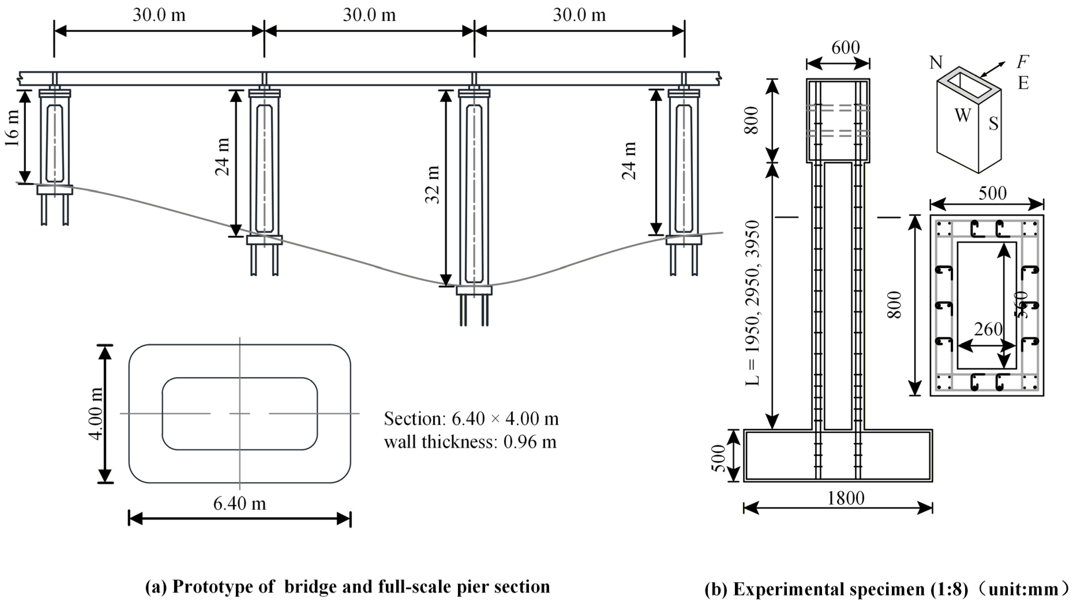
The experimental program comprised seven one-eighth-scale rectangular RC hollow-pier specimens, designated G1–G3, H1–H2, and I1–I2. The specimens were originally tested by the same research team, and the primary experimental results were reported in [26]. In the present study, the experimental data were reanalyzed to support shear-sensitive model validation and subsequent bridge-level seismic and fragility analyses. The prototype bridge, full-scale pier cross-section, and geometric details of the scaled specimens are illustrated in Figure 1. The present work does not claim the original tests as new; the dataset is used here as a common experimental basis for a quantitative two-model assessment and the subsequent full-scale response and fragility analyses.

Each specimen consisted of an RC footing, a rectangular hollow-pier shaft, and a top loading block. All pier shafts had outer cross-sectional dimensions of 500 mm × 800 mm and inner dimensions of 260 mm × 560 mm. The resulting wall thickness was uniformly 120 mm. The section depth parallel to the lateral loading direction was 500 mm. The pier shafts and footings were cast using C40 concrete. HRB400 bars were used as longitudinal reinforcement, whereas 10 mm diameter HRB335 bars were used as stirrups and cross-ties. A constant axial-load ratio of 0.05 was maintained for all specimens. The detailed specimen parameters are summarized in

Table 1. Design parameters of the rectangular hollow-pier specimens.

Shape	Specimen	L (m)	Section Size (mm)	L/D	Longitudinal Rebar		Stirrup
					Layout	ρl (%)	s (mm)	ρsv (%)
Rectangular	G1	1.95	500 × 800	3.9	20φ12 + 16φ16	2.15	100	2.13
	G2	2.95		5.9	20φ12 + 16φ16	2.15	100	2.13
	G3	3.95		7.9	20φ12 + 16φ16	2.15	100	2.13
	H1	2.95		5.9	20φ12 + 16φ16	2.15	70	3.04
	H2	2.95		5.9	20φ12 + 16φ16	2.15	150	1.42
	I1	2.95		5.9	26φ12 + 6φ16	1.63	100	2.13
	I2	2.95		5.9	32φ12 + 16φ16	2.69	100	2.13

.

The specimens were derived from the prototype using a geometric scale factor of $S_L$ = 1/8. With the same material-strength scale adopted for the prototype and model, the stress, strain, and elastic modulus scale factors were taken as unity. The corresponding scale factors were 1/8 for displacement, eight for curvature, 1/64 for area and force, 1/512 for moment, and 1/8 for lateral stiffness. The applied axial force preserved the prototype axial-load ratio of 0.05, while the longitudinal and transverse reinforcement ratios were maintained using available bar sizes and spacings. Because the tests were quasistatic, mass, acceleration, and time similitude were not invoked.

All specimens shared the same outer and inner section dimensions, wall thickness, material grades, loading direction, and axial-load ratio. Therefore, the experimental variables were limited to the investigated shear-span and reinforcement ratios; the independent effects of section proportions, wall thickness, and axial load were outside the scope of this study.

Specimens G1–G3 formed the shear-span ratio group, in which only ($\mathsf{\lambda }$) varied. Specimens H1, G2, and H2 formed the transverse reinforcement group, with different ${\rho }_{sv}$ values but identical geometry and longitudinal reinforcement. Specimens I1, G2, and I2 formed the longitudinal reinforcement group, with different ${\rho }_l$ values but identical geometry and transverse reinforcement. The specimen matrix therefore isolated the effects of $\lambda$, ${\rho }_{sv}$, and ${\rho }_l$.

2.2. Test Setup and Loading Protocol

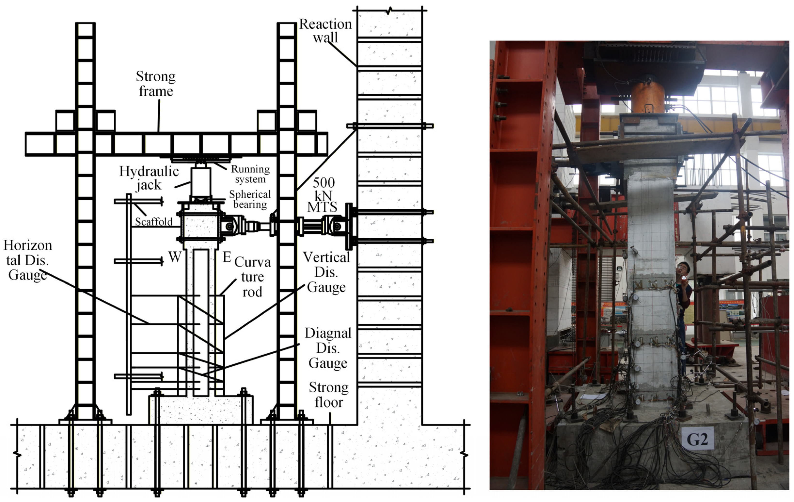
The tests were conducted at the Bridge Laboratory of the Highway Planning, Survey, Design and Research Institute of the Sichuan Provincial Department of Transport. Each specimen was anchored to the strong floor through its RC footing. A vertical hydraulic jack applied a constant axial load through a spherical hinge and movable loading system, maintaining an axial-load ratio of 0.05 while allowing lateral displacement at the pier top. The test setup is shown in Figure 2.

Reversed-cyclic lateral loading was applied at the pier top using a 500 kN MTS servo-controlled actuator (MTS Systems Corporation, Eden Prairie, MN, USA) with a stroke of ±250 mm. Lateral force and actuator displacement were recorded by the servo-control system. Bonded strain gauges measured the strains of the longitudinal bars, stirrups, and cross-ties, while concrete-surface strain gauges were installed in the potential plastic-hinge region. Horizontal displacement transducers were arranged along the pier height, curvature measurements were obtained at six elevations above the footing, and diagonal transducers monitored shear distortion. Additional horizontal and vertical displacement transducers on the footing measured rigid-body translation and rotation for displacement correction. The channels were recorded using an IMP data-acquisition system at 0.5 Hz. Crack initiation and propagation, concrete spalling, and reinforcement yielding were documented throughout the tests [26].

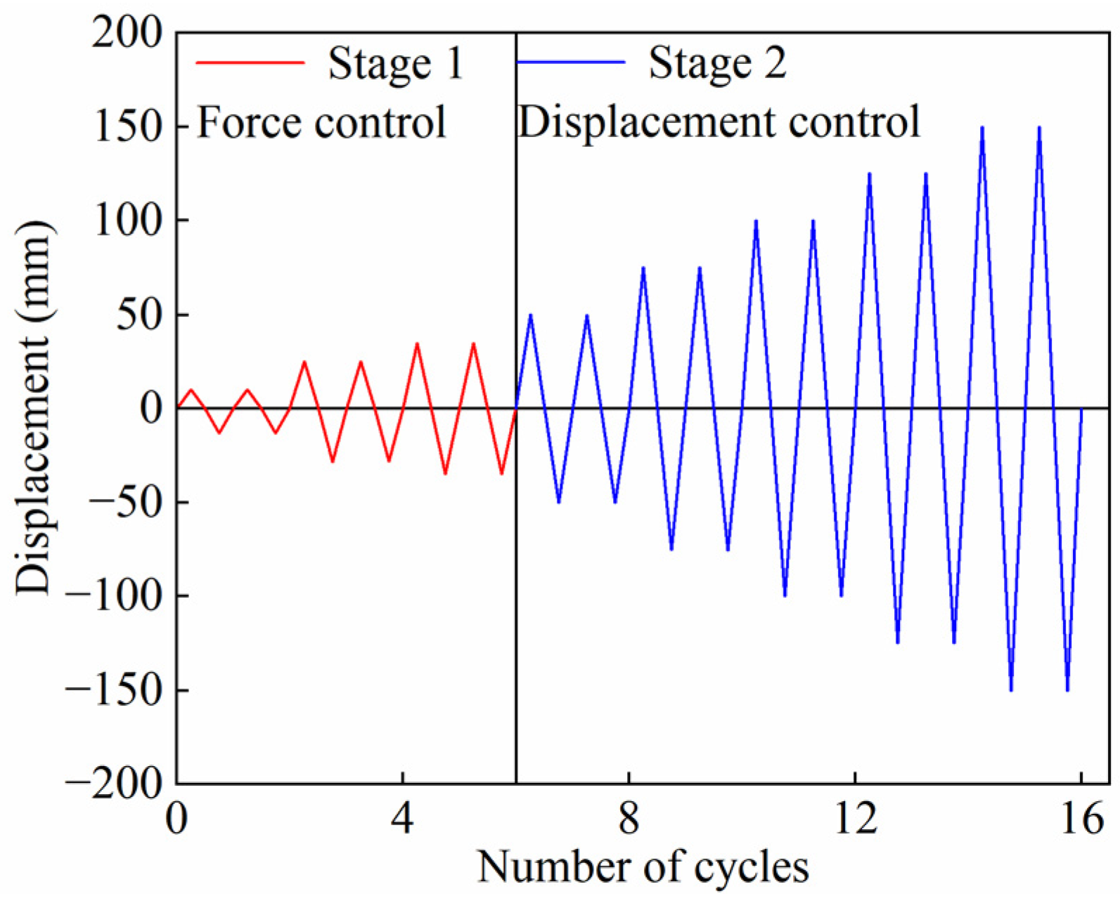
A hybrid force–displacement loading protocol was adopted and divided into two stages. During Stage I, the specimens were loaded under force control before yielding. The lateral force amplitude was progressively increased at each loading level and expressed as $i{F}_y$. Here, $F_y=M_y/L$ denotes the theoretical yield force, $M_y$ is the sectional yield moment, and $L$ is the pier height. The loading coefficient $i$ was selected within the range of 0.2–1.5. This stage continued until the specimen reached its actual yield condition. The corresponding pier-top displacement was defined as the yield displacement, ${\Delta }_y$. The force-control loading rate was 1 kN/s, and two fully reversed cycles were imposed at each force level; longitudinal-bar strain measurements were used to identify the first yield.

During Stage II, the loading mode was changed from force control to displacement control. The displacement amplitude was progressively increased in integer multiples of the yield displacement, expressed as $j{\Delta }_y$, where $j=\mathrm{1,2},3,\dots$. Two fully reversed cycles were imposed at each displacement level to characterize cyclic strength degradation, stiffness deterioration, and accumulated damage. Loading continued until the lateral load-carrying capacity decreased to approximately 80% of the previously attained peak resistance. This condition was adopted as the termination criterion for the test. The complete hybrid loading protocol is illustrated schematically in Figure 3. The displacement-control loading rate was 1 mm/s. This protocol followed the quasistatic procedure adopted for the original RC bridge-pier test program [26]. Because the specimens were reinforced concrete bridge piers rather than steel seismic-force-resisting components, the AISC 341 qualification protocol was not adopted.

For subsequent presentation and comparison, actuator pushing was defined as positive loading, whereas actuator pulling was defined as negative loading. The specimen face adjacent to the reaction wall was designated as the E face, and the opposite face was designated as the W face. The remaining two faces were designated as the N and S faces.

2.3. Damage Evolution and Failure Characteristics

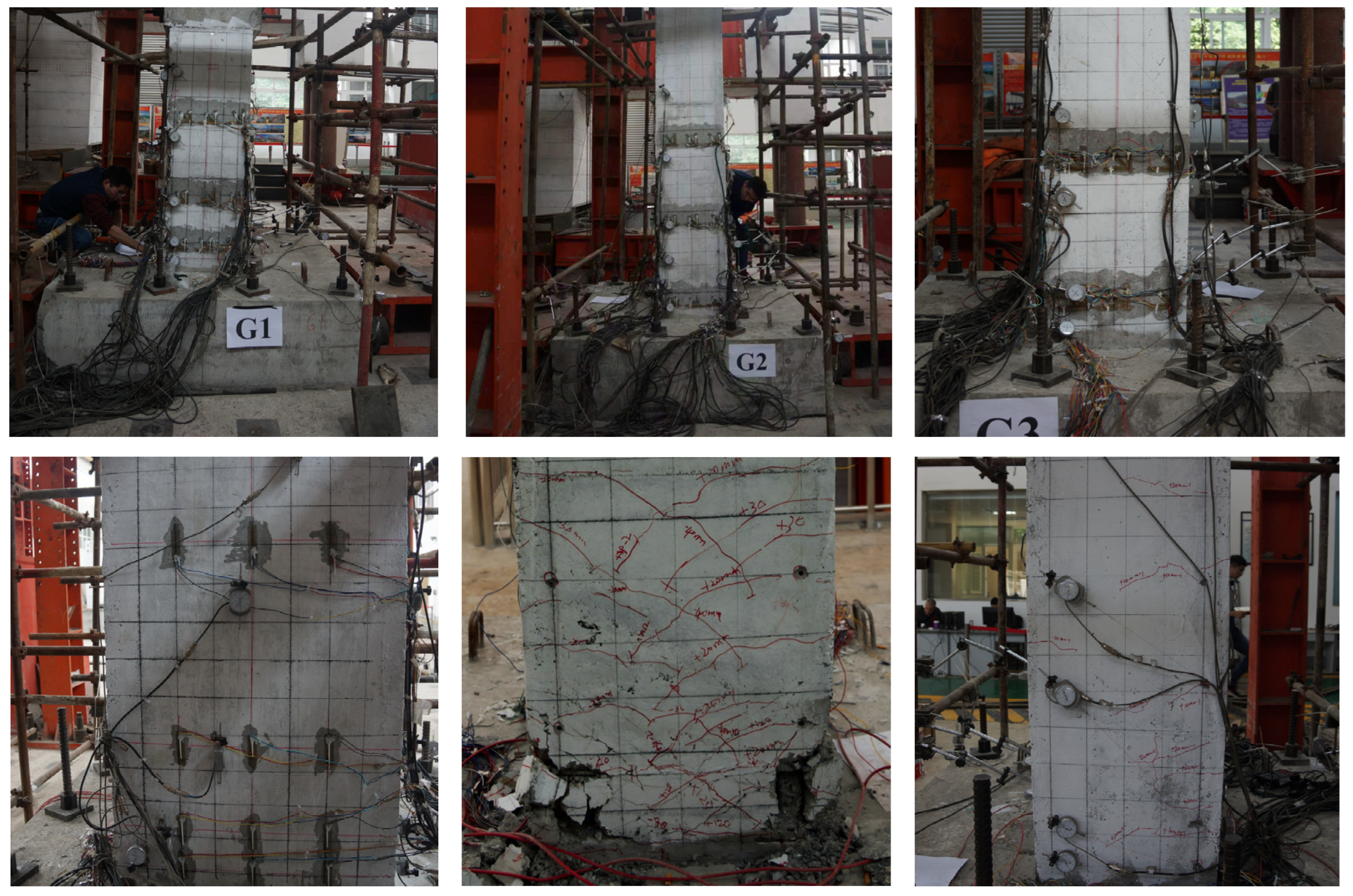
All seven rectangular RC hollow-pier specimens exhibited a similar damage progression, although the crack extent and localization varied among the parameter groups. Fine horizontal flexural cracks initially formed on the opposing E and W loading faces near the pier base. With increasing deformation, these cracks widened, propagated around the corners into the side walls, and gradually developed into diagonal cracks toward the compression side, indicating increased shear participation after flexural cracking. Representative damage photographs at different loading stages are shown in Figure 4.

The response of specimen G1 is used to illustrate the complete damage process. At a lateral load of 60 kN, a fine crack appeared near the construction joint on the E face. Under a reverse load of 90 kN, a structural crack approximately 0.05 mm wide formed on the W face, about 0.2 m above the footing. At a displacement amplitude of 5 mm, three and four flexural cracks were observed on the two loading faces, respectively, with widths of approximately 0.1 mm. As the displacement amplitude increased from 10 to 30 mm, the number of flexural cracks increased rapidly, the monitored main-crack width increased from 0.22 to 0.37 mm, and the cracking region extended to approximately half the pier height. During this stage, several horizontal flexural cracks propagated into the side walls and gradually developed into inclined shear-related cracks.

At displacement amplitudes of 45 and 60 mm, few new cracks formed, whereas the existing flexural and diagonal cracks continued to widen. The monitored main-crack widths reached 1.08 and 1.25 mm, and localized concrete peeling initiated near the pier base. At displacement amplitudes of 75 and 90 mm, intersecting diagonal cracks became increasingly evident on the side walls. The main-crack widths increased to 2.37 and 2.39 mm, accompanied by initial cover spalling and a reduction in lateral resistance. At 105 mm, cover spalling intensified, transverse reinforcement became exposed, and the longitudinal bars began to buckle. At the final loading stage, local concrete crushing, severe longitudinal-bar buckling, and occasional bar fracture occurred within the lower plastic-hinge region.

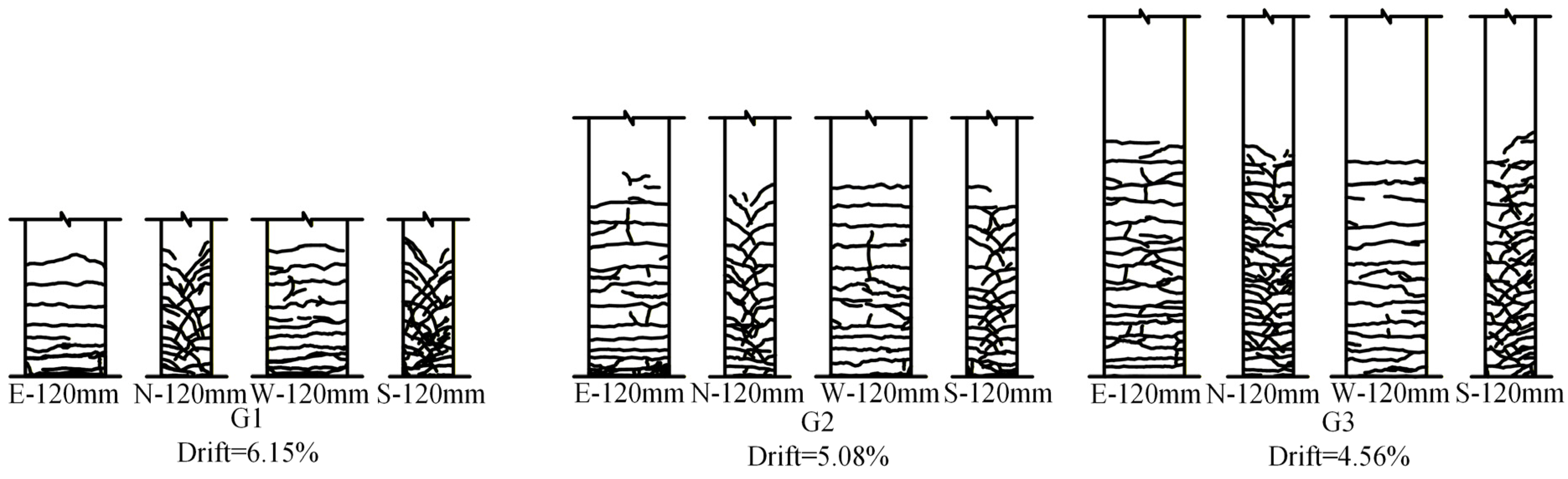
Across the specimen series, most new flexural cracks formed before approximately two to three times the yield displacement. Beyond this range, damage development was governed mainly by the widening and localization of several dominant cracks near the pier base. Cracks extending from the loading faces into the side walls were initially nearly horizontal but gradually propagated diagonally toward the compression side and intersected with cracks formed during reverse loading. Near and beyond peak resistance, concrete peeling, vertical corner cracking, cover spalling, and local crushing became concentrated in the lower pier region. The final crack distributions of specimens G1–G3 are shown in Figure 5.

The G-series specimens showed that $\mathsf{\lambda }$ strongly influenced the balance between flexural and shear-related damage. G1 exhibited extensive propagation and intersection of diagonal cracks over the lower side walls, forming a dense flexure–shear crack pattern near the pier base. G2 developed a mixed pattern of dominant horizontal flexural cracks and evident diagonal side-wall cracks, whereas G3 showed more regularly distributed horizontal cracks and less pronounced diagonal damage. The main-crack widths at the medium and severe damage boundaries were 1.25 and 2.39 mm for G1, 1.12 and 2.31 mm for G2, and 1.10 and 2.20 mm for G3, respectively. These results indicate that decreasing $\lambda$ increased shear participation and promoted localized flexure–shear deterioration.

Comparisons among H1, G2, and H2 showed that transverse reinforcement primarily affected crack widening and damage localization. H1, with the highest transverse reinforcement ratio, provided the most effective restraint against diagonal-crack widening and local concrete deterioration. Its main-crack widths at the medium and severe damage boundaries were 1.05 and 2.12 mm, respectively, compared with 1.36 and 2.40 mm for H2, which had the lowest transverse reinforcement ratio. Increasing ${\rho }_s$ therefore improved crack control and delayed localized deterioration but did not eliminate shear-related cracking.

Comparisons among I1, G2, and I2 showed that longitudinal reinforcement affected both flexural resistance and the force transferred through the hollow webs. The main-crack widths at the medium and severe damage boundaries were 1.00 and 2.20 mm for I1, 1.12 and 2.31 mm for G2, and 1.45 and 2.42 mm for I2, respectively. The larger crack widths of I2 indicate that increasing ${\mathsf{\rho }}_l$ did not suppress damage in the hollow webs. Although a higher ${\rho }_l$ increased the mobilized flexural resistance, it also maintained substantial shear demand, resulting in evident diagonal cracking and localized compression damage at large deformation levels.

Overall, decreasing $\lambda$ increased shear participation and damage localization, whereas increasing ${\rho }_{sv}$ restrained crack widening and delayed local deterioration. Increasing ${\rho }_l$ enhanced flexural resistance but did not reduce shear-related damage in the hollow webs. Among these parameters, $\lambda$ had the most evident influence on the transition from predominantly flexural cracking to localized flexure–shear deterioration.

2.4. Hysteretic Responses and Skeleton Curves

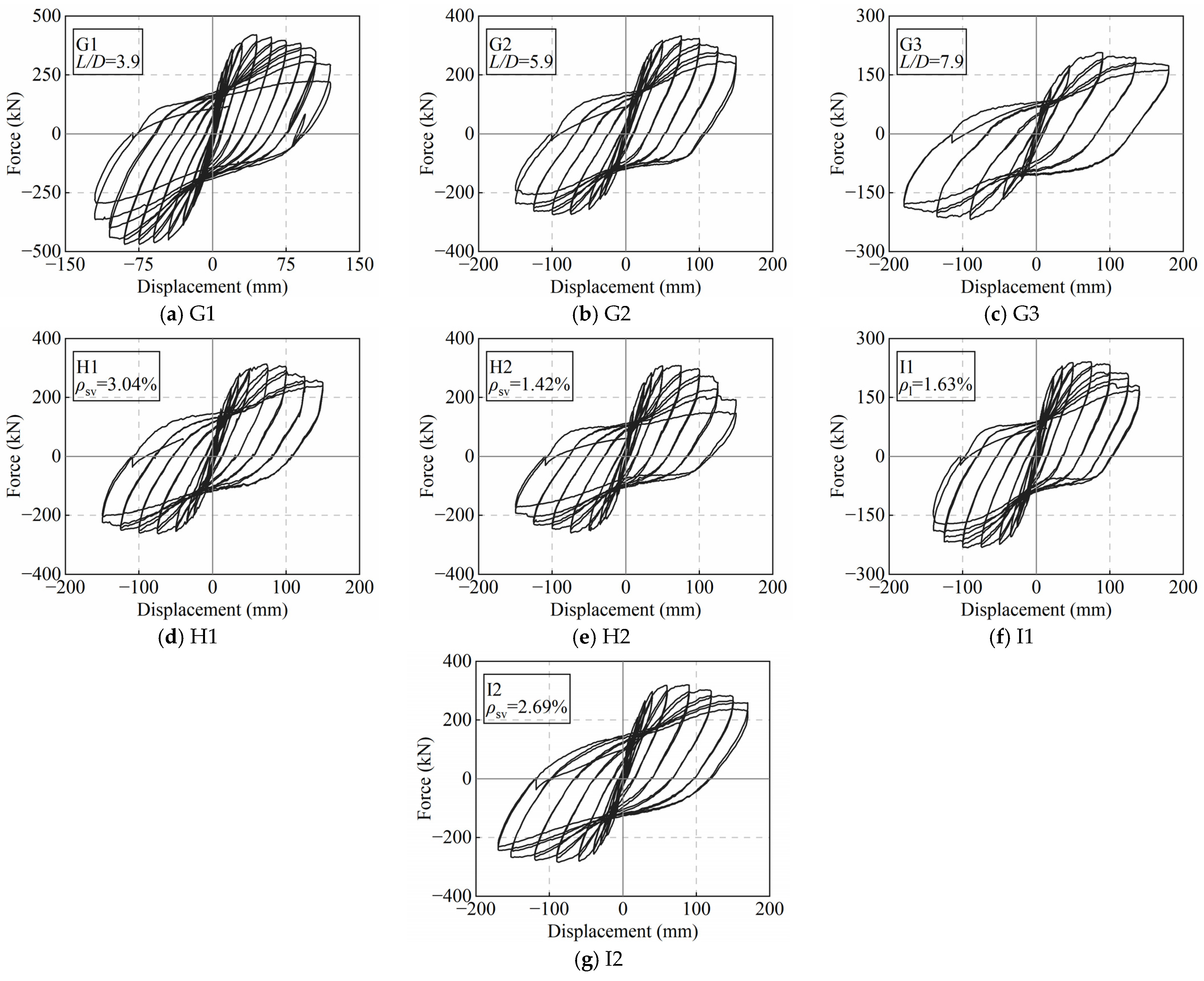
The measured lateral load–displacement hysteretic responses of the seven rectangular RC hollow-pier specimens are presented in Figure 6. At small displacement amplitudes, all specimens exhibited an approximately linear response with narrow hysteretic loops and limited residual deformation. After yielding of the longitudinal reinforcement, the loops gradually expanded and showed increasingly evident pinching around the origin. Repeated cycles at the same displacement level caused progressive reductions in lateral resistance and unloading stiffness. Strength degradation became more pronounced at large displacement amplitudes as flexural cracking, diagonal cracking, and concrete deterioration accumulated.

The hysteretic responses were generally stable before the peak lateral resistance was reached. No abrupt strength loss was observed during the initial nonlinear stage. After the peak, the resistance decreased progressively with increasing displacement amplitude. The positive and negative responses showed different degrees of asymmetry, particularly for G1, G2, H1, H2, and I2. This asymmetry became more evident during the post-peak stage because damage accumulated differently on the opposing loading faces.

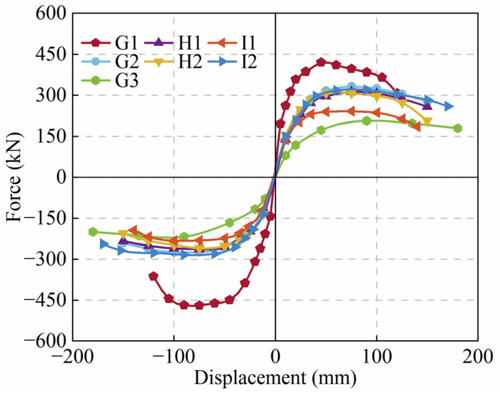
The skeleton curves were extracted separately from the positive and negative half-cycle responses. For each displacement level, the maximum positive and negative lateral load across the repeated cycles were retained. Incomplete unloading branches occurring at the end of the loading history were excluded. The resulting experimental skeleton curves of all seven specimens are compared in Figure 7.

All experimental skeleton curves exhibited three stages: an initial ascending branch, a gradually flattening post-yield branch, and a descending branch after peak resistance. The transition between these stages was strongly influenced by $\lambda$ and the reinforcement configuration.

For comparison, the mean peak lateral resistance was defined as:

$$F_p={\displaystyle \frac{F_p^{+}+\left|F_p^{-}\right|}{2}}$$

(1)

where $F_p^{+}$ and $F_p^{-}$ are the positive and negative peak lateral resistances, respectively. The terminal strength-retention ratio was calculated as the average of the positive and negative ratios between the resistance at the maximum displacement and the corresponding peak resistance.

The G-series specimens showed a strong dependence on $\lambda$. As $\lambda$ increased from 3.9 to 5.9 and 7.9, $F_p$ decreased from 445.0 to 303.3 and 212.3 kN, corresponding to reductions of 31.8% from G1 to G2 and 30.0% from G2 to G3. The peak resistance of G3 was 52.3% lower than that of G1. However, G1 exhibited the most pronounced post-peak degradation, with a terminal strength-retention ratio of 75.2%, compared with 85.2% for G2 and 89.4% for G3. Thus, decreasing $\lambda$ substantially increased lateral resistance but reduced post-peak stability, consistent with the more localized flexure–shear damage observed in G1.

The mean peak resistances of H1, G2, and H2 were 288.0, 303.3, and 283.7 kN, respectively, with a maximum difference of less than 7%. Therefore, ${\rho }_{sv}$ had only a limited effect on peak resistance within the investigated range. Its influence was more evident after the peak: the terminal strength-retention ratios were 85.8%, 85.2%, and 73.2% for H1, G2, and H2, respectively. Reducing ${\mathsf{\rho }}_{sv}$ to 1.42% therefore accelerated strength degradation and reduced post-peak stability, consistent with the more severe localized deterioration of H2.

For I1, G2, and I2, increasing the longitudinal reinforcement ratio, ${\rho }_l$, from 1.63% to 2.15% increased the mean peak resistance, $F_p$, from 236.7 to 303.3 kN, representing an increase of 28.1%. However, a further increase in ${\rho }_l$ to 2.69% resulted in an $F_p$ of 302.0 kN, which was approximately 0.4% lower than that of G2. The corresponding terminal strength-retention ratios were 80.3%, 85.2%, and 83.4%. These results indicate that increasing ${\rho }_l$ beyond 2.15% provided no further improvement in either peak resistance or post-peak stability, suggesting that the contribution of longitudinal reinforcement became limited by other governing mechanisms.

Overall, $\lambda$ had the strongest influence on both peak resistance and post-peak degradation, whereas ${\rho }_{sv}$ primarily affected post-peak stability. Increasing ${\rho }_l$ enhanced lateral resistance only within a limited range. These results confirm that the response of rectangular RC hollow piers cannot be characterized by flexural resistance alone and provide the experimental basis for the numerical models developed in Section 3.

3. Numerical Modeling and Validation

3.1. Modeling Strategies for the Pier Columns

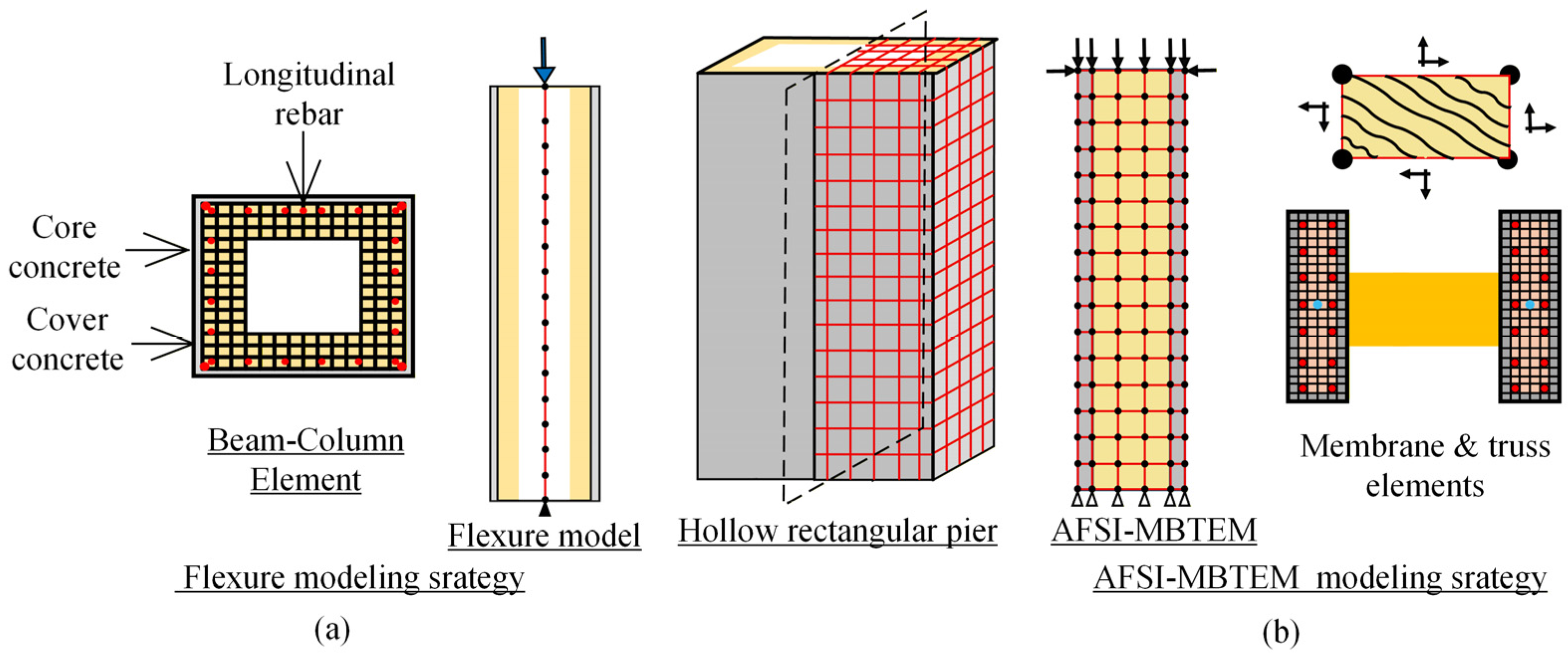
Two planar nonlinear models were established in OpenSees (version 3.8.0) to reproduce the in-plane reversed-cyclic response of the seven rectangular hollow-pier specimens [27]. The flexure model used a centerline fiber beam–column idealization, whereas the axial–flexure–shear interaction membrane–beam–truss element model (AFSI–MBTEM) separated the flexure-dominant boundary walls from the shear-dominant webs. The latter formulation was developed first for RC wall-type members and then extended to thin-walled hollow bridge piers [10,11]. As shown schematically in Figure 8, the two models used the same specimen geometry, measured material properties, total axial load, base restraint, and prescribed top displacement history. Their comparison, therefore, primarily reflects the different element formulations and the explicit treatment of web shear deformation in AFSI–MBTEM. All numerical inputs were assigned a priori from the measured specimen properties, and no specimen-specific parameter calibration or tuning was performed using the measured hysteretic responses.

In the flexure model, the hollow section was discretized into confined concrete, unconfined cover concrete, and longitudinal steel fibers according to the measured reinforcement layout. Fiber strains were determined from the sectional deformation, and the corresponding stresses were integrated to obtain the axial force and bending moment [28]. The fiber sections were assigned to displacement-based beam–column elements with numerical integration along the pier height, while a P–Delta transformation accounted for geometric nonlinearity [29]. This formulation efficiently represents distributed axial–flexural yielding but does not include web shear strain as an independent deformation mode.

Concrete01 was used for the confined and unconfined concrete fibers. This material follows the Kent–Scott–Park compressive envelope and Karsan–Jirsa unloading–reloading rules and neglects concrete tensile resistance [29,30]. The confined concrete parameters were determined with reference to the Mander model [31]. Longitudinal reinforcement was modeled using ReinforcingSteel, which represents yielding, the yield plateau, strain hardening, the Bauschinger effect, cyclic fatigue, and strength degradation [32]. Thus, the flexure model captures the principal uniaxial concrete and steel mechanisms governing axial–flexural response without introducing an empirical shear spring.

AFSI–MBTEM follows the membrane representation of cracked RC under in-plane loading. In membrane theory, average normal and shear strains are coupled through equilibrium, compatibility, and constitutive relationships. Transverse cracking reduces the effective compressive resistance of concrete, while orthogonal reinforcement continues to transfer tensile forces [33,34]. These concepts provide the mechanical basis for representing diagonal compression fields, distributed reinforcement, and axial–flexure–shear interactions. In AFSI–MBTEM, they are implemented through a damage–plasticity membrane–beam–truss assembly rather than through a separate empirical shear model.

The AFSI–MBTEM section was decomposed according to the observed damage pattern. The E and W boundary walls, dominated by the axial–flexural response, were modeled using displacement-based fiber beam–column elements, while the N and S webs, where inclined cracking and shear distortion developed, were combined into an equivalent plane-stress strip. The strip thickness equaled the sum of the two physical web thicknesses, and the corresponding horizontal and vertical reinforcement areas were aggregated into orthogonal ReinforcingSteel trusses. Four-node membrane elements using PlasticDamageConcretePlaneStress represented the web concrete, including multiaxial damage–plasticity, compression softening, and cyclic stiffness and strength degradation [11,35]. Three membrane elements were used across the web strip, with longitudinal subdivisions adjusted to control the element aspect ratio.

The membrane and truss elements shared nodes, imposing strain compatibility and perfect bond within the equivalent web. Boundary-wall, membrane, and truss nodes were aligned at common elevations and tied through shared translational degrees of freedom or equalDOF constraints, while stiff elastic links at the base and loading level distributed axial force and lateral displacement. This assembly preserves equilibrium and deformation compatibility between the axial–flexural boundary walls and axial–shear web while allowing the web shear strain to evolve as an independent deformation component [11,35].

Both models used identical boundary conditions, loading protocols, and post-processing procedures. The footing was fixed, and foundation flexibility and strain-penetration effects were neglected. The axial load was applied incrementally and then maintained while the measured reversed-cyclic displacement history was imposed at the pier top. Pier-top displacement and lateral resistance were extracted directly, and the hysteretic and skeleton curves, yield response, peak strength, effective stiffness, residual displacement, and hysteretic energy were evaluated consistently. The flexure model served as the axial–flexural baseline, whereas AFSI–MBTEM quantified the effects of explicit web shear deformation and axial–flexure–shear interaction.

3.2. Comparison Between Experimental and Numerical Results

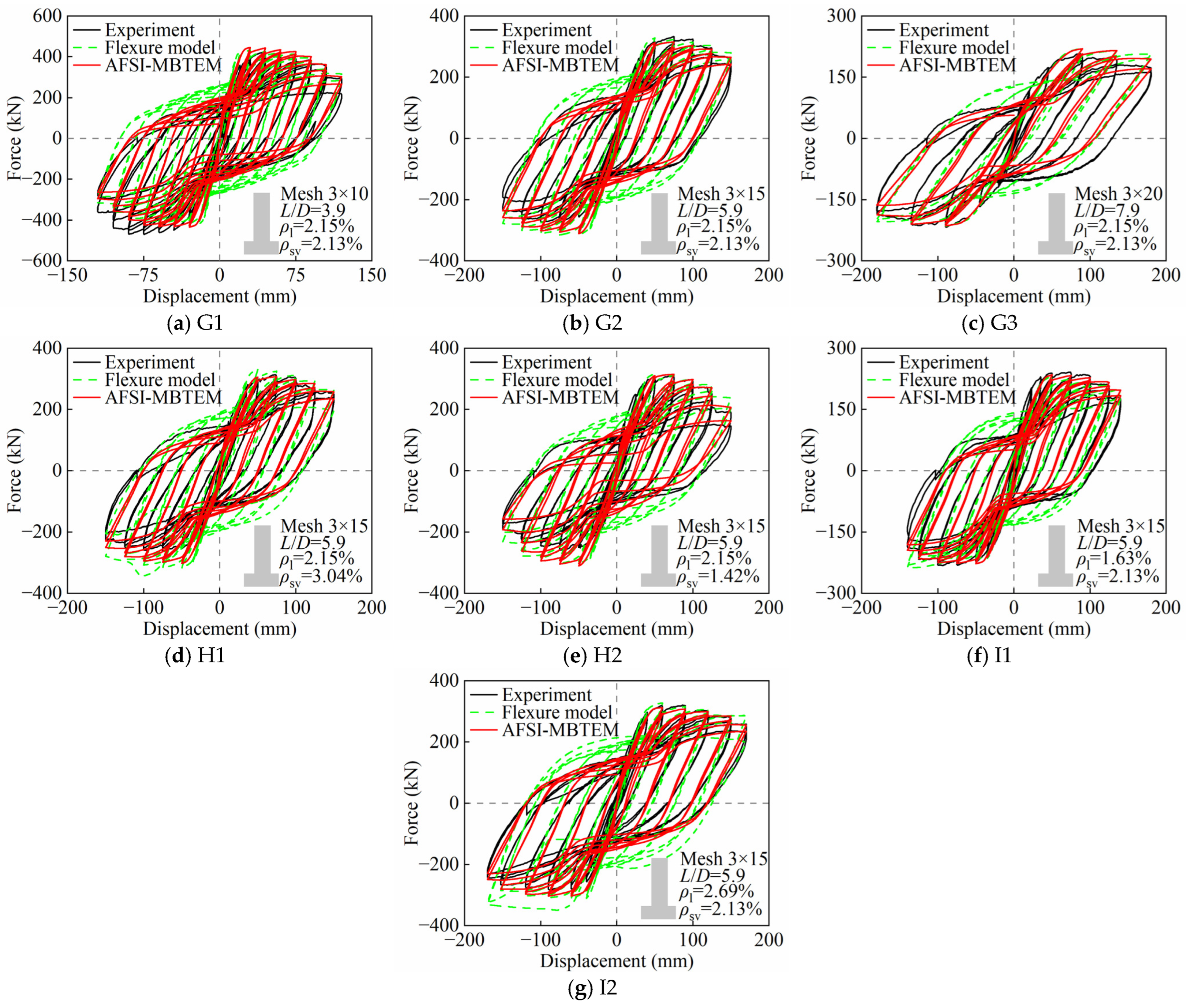
The two numerical models were subjected to the same displacement histories used in the cyclic tests. Figure 9 compares the measured hysteretic responses with those predicted by the flexure model and AFSI–MBTEM. The comparison considers the initial response, yielding transition, unloading and reloading paths, pinching behavior, peak strength, and post-peak deterioration.

Both models reproduced the overall force–displacement response, including the transition from approximately linear behavior to yielding and subsequent strength degradation. Their differences became more evident after yielding and at large displacement amplitudes. The flexure model generally produced wider hysteresis loops and higher reloading forces, thereby underestimating pinching and overestimating hysteretic energy dissipation. In contrast, AFSI–MBTEM more closely reproduced the measured unloading–reloading paths and the progressive contraction of the hysteresis loops.

For G1–G3, both models captured the reduction in lateral strength with increasing $\mathsf{\lambda }$. The measured mean peak strengths were 444.96, 303.30, and 212.31 kN. The corresponding predictions were 439.63, 312.78, and 216.64 kN for AFSI–MBTEM and 425.83, 321.91, and 217.82 kN for the flexure model. The improvement provided by AFSI–MBTEM was most evident for G1, which had the lowest $\lambda$ and the strongest post-peak deterioration. Its mean peak-strength error decreased from 4.30% to 1.20%. The corresponding error for G2 decreased from 6.14% to 3.13%, whereas both models predicted the peak strength of G3 within 3%. AFSI–MBTEM also reproduced the ascending and descending branches more accurately.

The comparisons among H1, G2, and H2 showed that AFSI–MBTEM better captured the effects of transverse reinforcement on pinching and post-peak deterioration. For H1, the mean peak-strength error decreased from 17.02% for the flexure model to 5.83% for AFSI–MBTEM, which also followed the unloading paths more closely. For H2, both models overestimated the mean peak strength, with corresponding errors of 9.40% and 10.21%. Although AFSI–MBTEM did not improve the peak-strength prediction for H2, it reproduced the positive descending branch more accurately. Its predicted positive terminal strength-retention ratio was 0.678, close to the experimental value of 0.671. The larger discrepancy in the negative direction indicates that the directional deterioration of H2 was not fully captured.

For I1, both models predicted the peak strength satisfactorily. The mean peak-strength errors were 1.13% for the flexure model and 2.38% for AFSI–MBTEM, although AFSI–MBTEM better reproduced the overall skeleton-curve shape and post-yield response. For I2, the flexure model substantially overestimated the negative peak strength, with an error of 22.97%, compared with 6.68% for AFSI–MBTEM. Consequently, the mean peak-strength error decreased from 11.94% to 1.87%.

Across the seven specimens, the mean absolute peak-strength error decreased from 7.50% for the flexure model to 3.81% for AFSI–MBTEM. The mean skeleton-curve nRMSE, calculated at matched displacement points and normalized by the experimental peak absolute force, decreased from 11.28% to 7.70%, with AFSI–MBTEM producing a lower value for every specimen. These results indicate that model performance should be evaluated using the complete response rather than peak strength alone.

Some discrepancies remained in local cycle-to-cycle fluctuations, directional asymmetry, and the terminal response after severe damage. Nevertheless, AFSI–MBTEM provided a more balanced representation of strength, pinching, stiffness degradation, and post-peak deterioration than the flexure model.

3.3. Assessment of Model Accuracy and Applicability

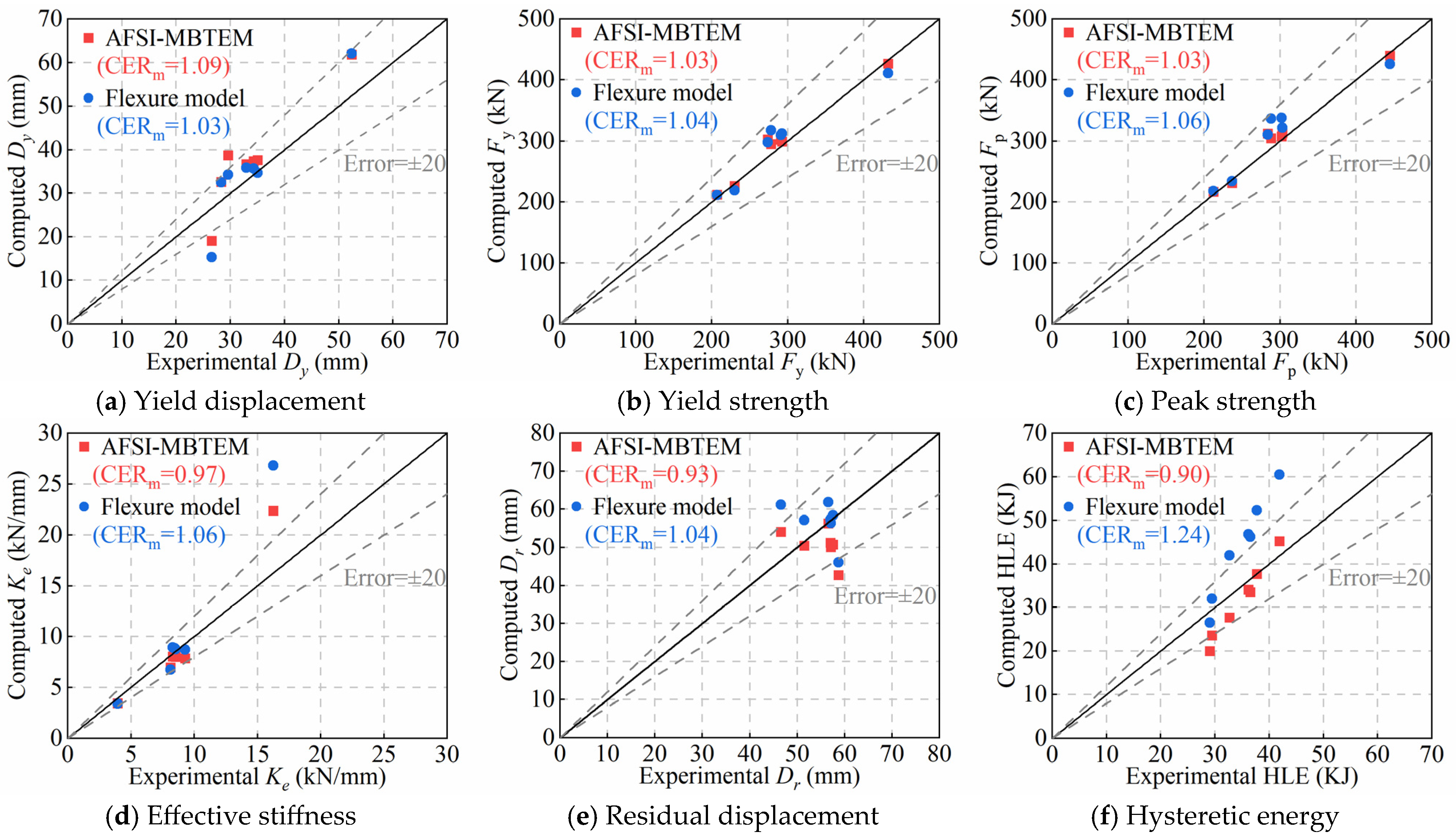
To supplement the comparisons of the hysteretic and skeleton curves, the predictive accuracy of the two numerical models was quantitatively evaluated using six response indices: yield displacement $D_y$, yield strength $F_y$, peak strength $F_p$, effective stiffness $K_e$, residual displacement $D_r$, and hysteretic loop energy (HLE). The residual displacement and HLE were represented by the mean values obtained at the nominal displacement levels common to the experiment and the two numerical models. Displacement levels below 40 mm were excluded because the relative errors of the residual displacement and loop area were highly sensitive to small measurement and numerical offsets within the approximate elastic response range. For each specimen and response index, the computed-to-experimental ratio was defined as:

$${\mathrm{C}\mathrm{E}\mathrm{R}}_i={\displaystyle \frac{R_{i,\mathrm{c}\mathrm{a}\mathrm{l}}}{R_{i,\mathrm{e}\mathrm{x}\mathrm{p}}}}$$

(2)

where $R_{i,\mathrm{c}\mathrm{a}\mathrm{l}}$ and $R_{i,\mathrm{e}\mathrm{x}\mathrm{p}}$ denote the calculated and experimental values, respectively. The mean computed-to-experimental ratio ${\mathrm{C}\mathrm{E}\mathrm{R}}_m$, coefficient of variation (COV), mean absolute error (MAE), and root-mean-square error (RMSE) were employed to characterize the prediction bias and dispersion. A value of ${\mathrm{C}\mathrm{E}\mathrm{R}}_m$ close to unity indicates limited systematic bias, whereas lower MAE and RMSE values indicate greater overall accuracy. The calculated and experimental results are compared in Figure 10, in which the solid line denotes perfect agreement and the dashed lines define the ±20% error band.

Both models predicted yield and peak strengths with reasonable accuracy. For the flexure model, the ${\mathrm{C}\mathrm{E}\mathrm{R}}_m$ values for $F_y$ and $F_p$ were 1.041 and 1.060, with MAEs of 6.89% and 7.50%, respectively. For AFSI–MBTEM, the corresponding ${\mathrm{C}\mathrm{E}\mathrm{R}}_m$ values were 1.032 and 1.028, and the MAEs decreased to 4.00% and 3.81%. All strength predictions remained within the ±20% error band, indicating that both models reproduced lateral resistance satisfactorily, although AFSI–MBTEM provided greater accuracy and consistency.

The differences were more evident for deformation- and stiffness-related indices. The $D_y$ MAEs were 15.11% for the flexure model and 17.19% for AFSI–MBTEM, indicating no systematic improvement in yield displacement prediction. This result may partly reflect the sensitivity of the equivalent-energy yield point to the post-peak skeleton-curve shape. In contrast, AFSI–MBTEM improved the prediction of $K_e$, with ${\mathrm{C}\mathrm{E}\mathrm{R}}_m=0.971$, MAE = 13.63%, and RMSE = 17.36%, compared with ${\mathrm{C}\mathrm{E}\mathrm{R}}_m=1.061$, MAE = 16.66%, and RMSE = 26.22% for the flexure model. For G1, the effective stiffness error decreased from approximately 64.9% to 37.5%.

The benefits of axial–flexure–shear interaction were most evident for G1, which had the lowest $\lambda$. AFSI–MBTEM reduced the errors in all six response indices relative to the flexure model. In particular, the HLE error decreased from approximately 40.8% to 5.1%, while the $D_r$ error decreased from 31.1% to 15.5%. These improvements indicate that the pinching, shear deformation, and cyclic energy-dissipation mechanisms of low-$\lambda$ hollow piers cannot be adequately represented by a purely flexural formulation.

For G3, the strength predictions of the two models were comparable, and the influence of shear interaction was less pronounced. AFSI–MBTEM underestimated $D_r$ and HLE by approximately 24.7% and 32.6%, respectively, whereas the corresponding errors of the flexure model were 19.4% and 11.3%. This result suggests that G3 was predominantly flexure-controlled, and that the benefits of AFSI–MBTEM depend on the relative contribution of shear deformation rather than increasing uniformly across all $\lambda$ values.

Across all specimens, the two models provided comparable predictions of $D_r$. The flexure model yielded ${\mathrm{C}\mathrm{E}\mathrm{R}}_m=1.044$ and an MAE of 10.44%, whereas AFSI–MBTEM yielded ${\mathrm{C}\mathrm{E}\mathrm{R}}_m=0.930$ and an MAE of 11.43%. Although AFSI–MBTEM produced a slightly lower RMSE and placed six of the seven predictions within the ±20% band, it did not provide a consistent improvement in MAE. A clearer improvement was observed for HLE: the MAE decreased from 23.57% to 13.29%, and the RMSE decreased from 26.30% to 16.62%. The flexure model generally overestimated HLE ${\mathrm{C}\mathrm{E}\mathrm{R}}_m=1.204$, whereas AFSI–MBTEM moderately underestimated it ${\mathrm{C}\mathrm{E}\mathrm{R}}_m=0.822$.

Overall, the flexure model reproduced lateral strength and residual displacement reasonably well but tended to overestimate effective stiffness and hysteretic energy, particularly for specimens with greater shear participation. AFSI–MBTEM improved the predictions of $F_y$, $F_p$, $K_e$, and HLE and provided the greatest benefit for the low-$\mathsf{\lambda }$ specimen G1. Its advantages were less consistent for $D_y$ and for the residual deformation and energy dissipation of G3. Within the seven-specimen dataset, AFSI–MBTEM provided greater benefits for cases with appreciable shear participation, whereas the flexure model remained adequate for the more flexure-dominated cases. This comparison is limited to the tested section geometry, wall thickness, axial-load ratio, and reinforcement ranges.

4. Cyclic and Seismic Response Analysis of Full-Scale Bridge Piers

4.1. Dynamic Characteristics

A complete full-scale model of the prototype bridge described in Section 2.1 was established to determine its global longitudinal dynamic characteristics and common reference period. The flexure and AFSI–MBTEM formulations were implemented in OpenSees using identical geometry, mass distribution, material properties, axial loads, boundary conditions, and damping assumptions. An independent SAP2000 model with the same global configuration was established for comparison. The calculated natural periods are presented in

Table 2. Comparison of the first three natural periods obtained using the OpenSees and SAP2000 models.

Mode	OpenSees (Flexure) (s)	OpenSees (AFSI–MBTEM) (s)	SAP2000 (s)	Mean Period (s)
First mode, $T_1$	1.638	1.649	1.648	1.645
Second mode, $T_2$	1.259	1.267	1.269	1.265
Third mode, $T_3$	0.865	0.871	0.874	0.870

.

The SAP2000 model produced first-, second-, and third-mode periods of 1.648, 1.269, and 0.874 s, respectively. The maximum difference among the OpenSees and SAP2000 results was approximately 1.03%. Because the three models yielded closely consistent first longitudinal natural periods, their arithmetic mean, T₁ = 1.645 s, was adopted as the common reference period of the complete-bridge system for the longitudinal response analysis and the subsequent classification of pulse-like motions using $T_p/T_1$. Both OpenSees formulations showed close agreement with the SAP2000 model and were subsequently used in the cyclic and near-fault seismic analyses.

4.2. Cyclic Response Analysis

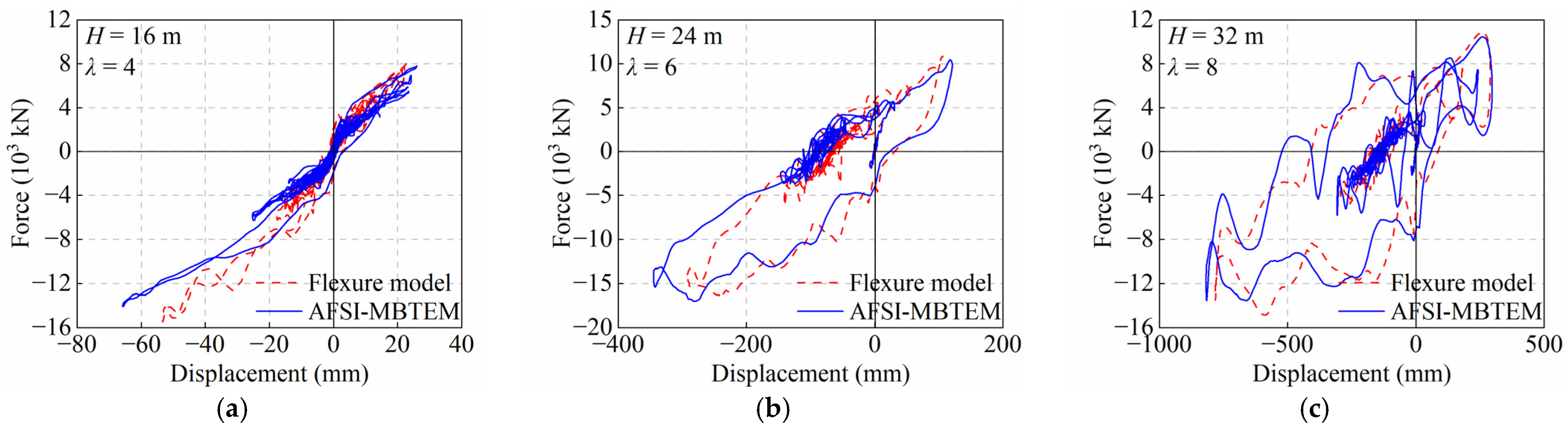
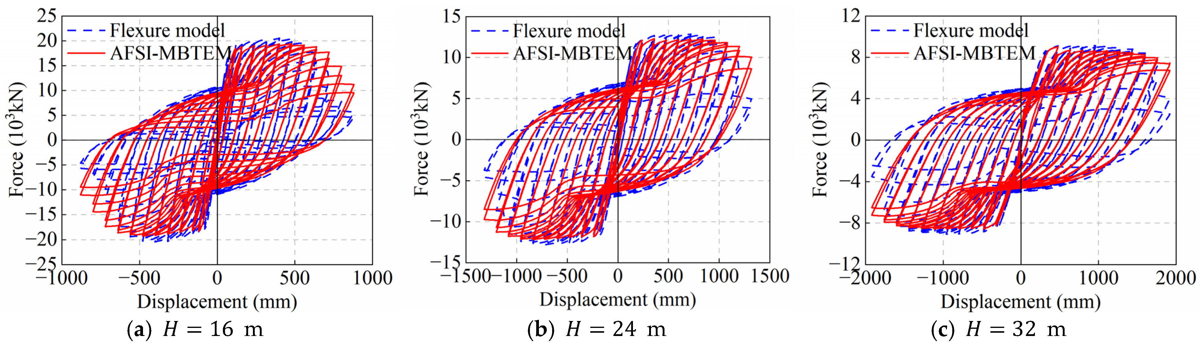
To investigate the influence of axial–flexure–shear interactions on the cyclic response of full-scale piers, three coupled height–shear-span configurations were considered: 16 m with $\mathsf{\lambda }=4$, 24 m with $\mathsf{\lambda }=6$, and 32 m with $\mathsf{\lambda }=8$. Across the three full-scale configurations, the prototype-section dimensions, wall thickness, reinforcement, material properties, axial-load ratio, and boundary conditions were held constant; only the pier height and resulting shear-span ratio varied together. For each configuration, the flexure model and AFSI–MBTEM used identical inputs. The same drift-controlled loading history was applied to both models. One cycle was imposed at drift ratios of 0.05%, 0.10%, and 0.20%, followed by two cycles at each subsequent level. The 16 and 24 m piers were loaded to 5.5% drift, corresponding to maximum displacements of 880 and 1320 mm, respectively, whereas the 32 m pier was further loaded to 6.0% drift, corresponding to 1920 mm. Both formulations completed their prescribed loading histories.

As shown in Figure 11, both models produced approximately symmetric hysteretic responses with clear stiffness reduction, pinching, and post-peak deterioration as the drift increased. At 0.05% drift, the secant stiffnesses predicted by the flexure model were 566.8, 206.3, and 99.7 kN/mm for the 16, 24, and 32 m piers, respectively, compared with 582.4, 215.9, and 103.6 kN/mm from AFSI–MBTEM. The differences of 2.8–4.6% indicate broadly consistent initial responses between the two formulations.

More evident differences developed after cracking. At drift ratios of 0.30% and 0.50%, the strengths predicted by AFSI–MBTEM were 17.5% and 15.0% lower than those of the flexure model for the 16 m pier. The corresponding reductions were 6.3% and 10.9% for the 24 m pier and 0.4% and 5.4% for the 32 m pier. This trend indicates that shear deformation contributed more strongly to the global displacement of the 16 m (λ = 4) coupled height–shear-span configuration.

The peak strengths predicted by the flexure model were 20.510, 12.874, and 9.133 MN, compared with 19.373, 12.286, and 9.018 MN from AFSI–MBTEM. These values represent reductions of 5.54%, 4.56%, and 1.26%. The decreasing discrepancy indicates that the influence of shear interaction on peak resistance became weaker as the pier height and shear-span ratio increased together.

At large drift, AFSI–MBTEM generally exhibited better strength retention. At the common drift ratio of 5.5%, the second-to-first-cycle strength ratios from the flexure model were 0.818, 0.791, and 0.808 for the 16, 24, and 32 m piers, respectively, compared with 0.853, 0.865, and 0.972 from AFSI–MBTEM. For the 32 m pier at 6.0% drift, the ratio decreased to 0.651 for the flexure model but remained 0.901 for AFSI–MBTEM. Thus, differences in the post-peak response remained evident even when the peak-strength predictions were similar.

Over the complete loading histories, AFSI–MBTEM predicted 1.4% greater cumulative hysteretic energy for the 16 m pier but 3.4% and 4.6% lower values for the 24 and 32 m piers. Therefore, the shear interaction did not produce a uniform change in energy dissipation. Overall, AFSI–MBTEM provided a more mechanically consistent representation of flexural and shear deformation. Its influence was most evident in the transition-stage resistance of the 16 m (λ = 4) coupled configuration and in the repeated-cycle stability under large deformation.

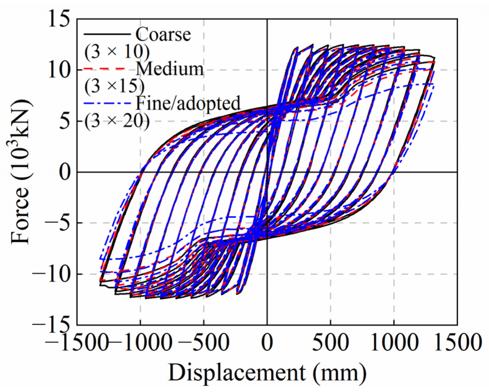
As shown in Figure 12,to assess mesh sensitivity in the shear-sensitive formulation, the 24 m pier was reanalyzed using AFSI–MBTEM membrane meshes of 3 × 10, 3 × 15, and 3 × 20. Because three elements were retained across the 3.04 m web strip, the corresponding nominal longitudinal element heights were 2.4, 1.6, and 1.2 m, giving height-to-width aspect ratios of 2.37, 1.58, and 1.18, respectively. Geometry, materials, reinforcement, axial-load ratio, loading history, and numerical settings were otherwise unchanged. Relative to the adopted 3 × 20 mesh, the 3 × 15 mesh differed by 0.46% in peak resistance, 1.31% in cumulative hysteretic energy up to 3% drift, and 3.41% in full-history energy; the nRMSE of the complete first-cycle envelope was 1.72%. The corresponding differences for the 3 × 10 mesh were 1.74% in peak resistance and 3.44% in complete-envelope nRMSE. The progressive stabilization of the global cyclic response indicates that the adopted mesh is sufficiently refined for the reported force–displacement and energy measures. Pointwise localized strain and damage fields are not interpreted as mesh-objective; the present assessment is limited to the global response quantities used in the model comparisons.

4.3. Seismic Response Analysis Under Near-Fault Ground Motions

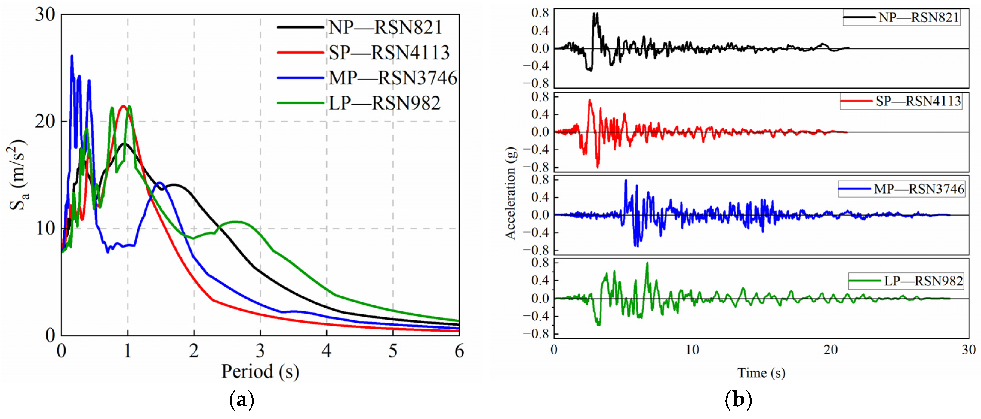
To examine the influence of axial–flexure–shear interaction on the nonlinear seismic response of full-scale hollow bridge piers, four representative near-fault ground motions were selected: NP–RSN821, SP–RSN4113, MP–RSN3746, and LP–RSN982. The pulse periods of the SP, MP, and LP records were 1.134, 1.967, and 3.157 s, respectively. Based on the common longitudinal reference period of the complete-bridge system, $T_1=1.645$ s, the corresponding $T_p/T_1$ ratios were 0.689, 1.196, and 1.919. The original PGA and PGV values were obtained from the PEER NGA-West2 database. Each record was normalized and scaled to PGA = 0.8 g for the nonlinear time-history analyses. Detailed record information is summarized in

Table 3. Characteristics of the representative ground motions selected for the nonlinear time-history analyses.

Type	RSN	Earthquake	${\mathit{M}}_{\mathit{w}}$	${\mathit{R}}_{\mathit{r}\mathit{u}\mathit{p}}$ (km)	${\mathit{V}}_{\mathit{S}30}$ (m/s)	PGA (m/s2)	PGV (m/s)	${\mathit{T}}_{\mathit{p}}$ (s)	${\mathit{T}}_{\mathit{p}}/{\mathit{T}}_1$
NP	821	Erzican, Turkey	6.69	4.38	352.05	4.364	0.938	–	–
SP	4113	Parkfield-02, CA	6.00	2.85	372.26	1.282	0.195	1.134	0.689
MP	3746	Cape Mendocino	7.01	18.31	459.04	4.449	0.504	1.967	1.196
LP	982	Northridge-01	6.69	5.43	373.07	5.141	0.976	3.157	1.919

, and the corresponding acceleration histories and 5%-damped response spectra are presented in Figure 13.

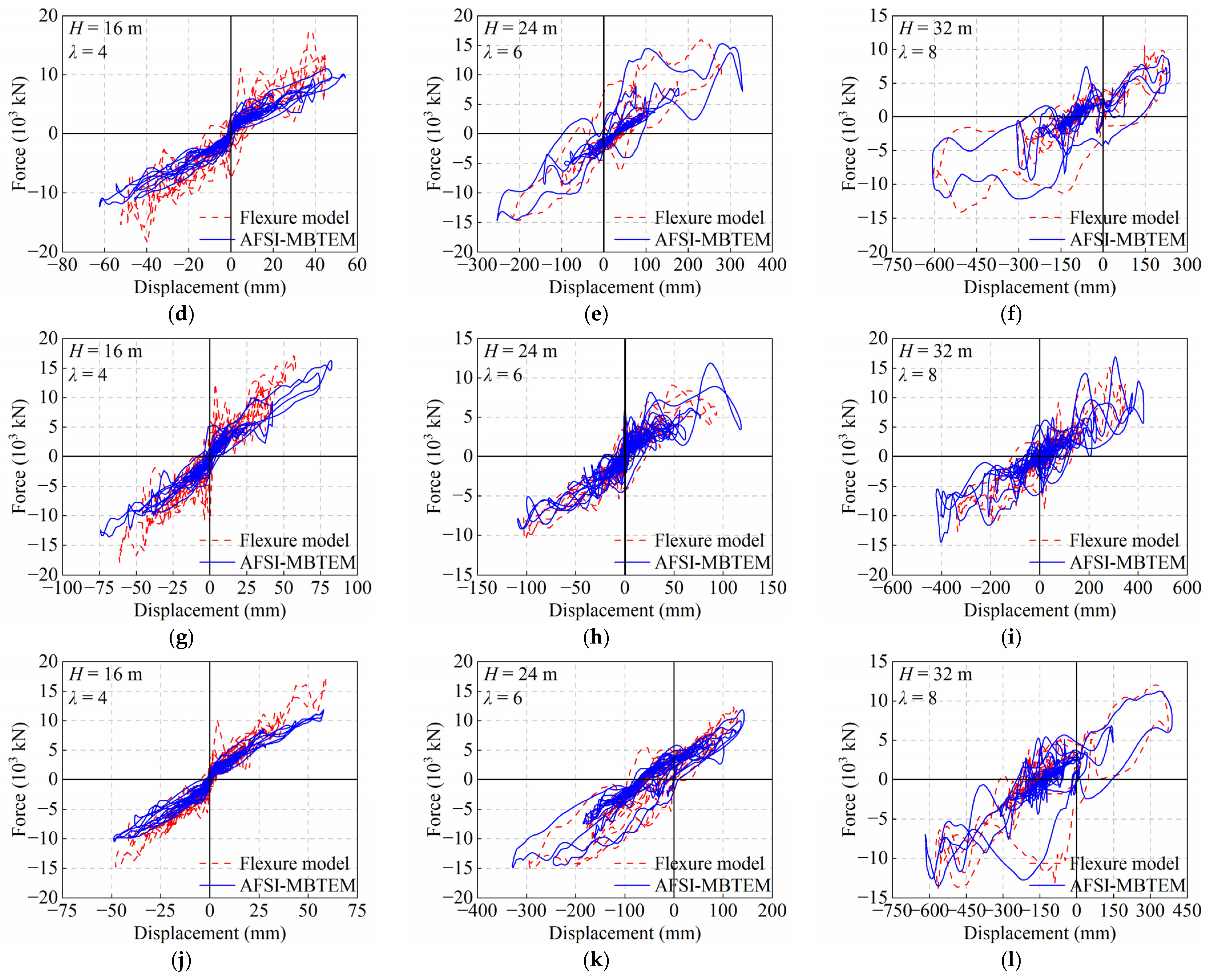
NP, SP, MP, and LP denote non-pulse, short-period pulse, medium-period pulse, and long-period pulse ground motions, respectively. $R_{rup}$ is the closest distance to the rupture plane, and $V_{S30}$ is the time-averaged shear-wave velocity over the upper 30 m of the site. The reported PGA and PGV values correspond to the original unscaled PEER records. Figure 14 compares the base-shear–pier-top displacement responses predicted by the flexure model and AFSI–MBTEM.

The nonlinear response-history analyses in Section 4.3 and Section 5 were performed on the independent 16, 24, and 32 m pier-level models; the complete-bridge model in Section 4.1 was used only to determine the common longitudinal reference period. The gravity-induced axial load was applied first and then maintained, tributary mass was represented by lumped masses at the pier-top nodes, and longitudinal ground acceleration was imposed at the fixed base using UniformExcitation. Rayleigh damping corresponding to 5% critical damping was defined from the first two modal frequencies. The equations of motion were integrated using the Newmark average-acceleration method (γ = 0.5 and β = 0.25) with a base time step of 0.005 s. Newton iteration and a NormDispIncr convergence test with a tolerance of 1.0 × 10⁻⁷ were used; alternative algorithms and time-step subdivision were invoked when required [11,35].

The largest base-shear differences occurred for the 16 m pier with $\lambda =4$. Relative to the flexure model, AFSI–MBTEM reduced the peak absolute base shear by 8.9%, 32.8%, 8.9%, and 31.5% under the NP, SP, MP, and LP records, respectively. Its effect on peak displacement was more record-dependent. The displacement increased from 53.27 to 65.77 mm under NP, from 52.44 to 62.41 mm under SP, and from 61.37 to 82.68 mm under MP, corresponding to increases of 23.5%, 19.0%, and 34.7%, respectively. Under LP, the displacement decreased slightly from 58.98 to 57.84 mm, or by 1.9%. Thus, shear interaction consistently reduced the peak force demand of the 16 m (λ = 4) coupled configuration, whereas its influence on displacement depended on the excitation.

For the 24 m pier with $\lambda =6$, AFSI–MBTEM increased the peak displacement under all four records. The increases were 17.8%, 18.0%, 14.8%, and 11.0% under NP, SP, MP, and LP, respectively. The corresponding peak drift ratios were 1.437%, 1.373%, 0.492%, and 1.371%, compared with 1.220%, 1.163%, 0.429%, and 1.235% from the flexure model. In contrast, the base-shear changes were comparatively limited under NP, SP, and LP, amounting to an increase of 1.7% and reductions of 4.5% and 1.8%, respectively. Under MP, however, AFSI–MBTEM increased the peak base shear by 12.7%. For this configuration, axial–flexure–shear interaction therefore affected displacement more consistently than peak force.

For the 32 m pier with $\lambda =8$, the two models produced similar peak displacements under SP excitation, with an increase of only 0.7% after the shear interaction was considered. The corresponding increases under NP and LP were 4.5% and 7.3%. A more evident difference occurred under MP, for which AFSI–MBTEM increased the peak displacement from 347.97 to 423.40 mm, or by 21.7%, and increased the peak base shear from 15.111 to 16.896 MN, or by 11.8%. Under NP, SP, and LP, the peak base shear decreased by 9.0%, 13.8%, and 2.0%, respectively. Therefore, although the two models generally converged for the slender configuration, appreciable differences remained under excitation with frequency content close to the bridge-system period.

The loop-integrated force–displacement work also varied with the coupled configurations and excitations. For the 16 m pier, AFSI–MBTEM increased the integrated work by 7.4% under NP, but reduced it by 4.7%, 4.5%, and 17.4% under SP, MP, and LP, respectively. For the 24 m pier, the changes were increases of 2.3% and 5.0% under NP and SP and reductions of 14.0% and 9.1% under MP and LP. For the 32 m pier, the corresponding changes were 5.0%, −15.1%, 23.1%, and −7.5%. These results indicate that peak displacement and loop-integrated work are not directly proportional because shear interaction modifies both the force level and the displacement trajectory.

The influence of AFSI–MBTEM depended jointly on the coupled height–shear-span configuration and the representative ground motion. Under SP excitation, the increase in peak displacement decreased from 19.0% for the 16 m configuration to 18.0% and 0.7% for the 24 and 32 m configurations, respectively. Under MP excitation, the corresponding increases were 34.7%, 14.8%, and 21.7%, whereas under LP excitation the displacement decreased by 1.9% for the 16 m pier but increased by 11.0% and 7.3% for the 24 and 32 m piers. The model effect therefore cannot be ranked solely according to pulse period or pier height.

These response trends are consistent with previous studies showing that explicit shear deformation can reduce lateral resistance while increasing deformation demand in thin-walled hollow piers [11,12]. The strong variation among records also agrees with findings that near-fault bridge response depends on pulse-period compatibility, spectral shape, and structural characteristics rather than on the pulse label alone [15,16,17]. Related studies further show that pulse-like demand may also vary with vertical-load level [24]. The present results extend these deterministic observations by showing that the influence of model formulation changes across the coupled height–shear-span configurations and can alter the representative record identified as critical.

The model formulation also altered the representative record governing displacement demand. MP produced the largest displacement of the 16 m pier for both models. For the 24 m pier, LP governed the flexure response, whereas NP governed the AFSI–MBTEM response. For the 32 m pier, NP remained governing for both formulations. Explicit consideration of shear interaction may therefore change both the magnitude of seismic demand and the representative record identified as critical.

Overall, AFSI–MBTEM did not produce a uniform increase in displacement or reduction in base shear. For $\lambda =4$, it consistently reduced peak base shear while substantially changing the displacement response. For $\lambda =6$, it primarily increased displacement demand, while its effect on peak base shear depended on the record. For $\lambda =8$, the two formulations generally converged, except under the MP record. These results demonstrate that the differences between the two models cannot be represented by a single correction factor. For the three investigated full-scale configurations, explicit axial–flexure–shear interactions could materially affect the record-dependent seismic response, although the magnitude and direction of these effects varied with the coupled configuration and excitation.

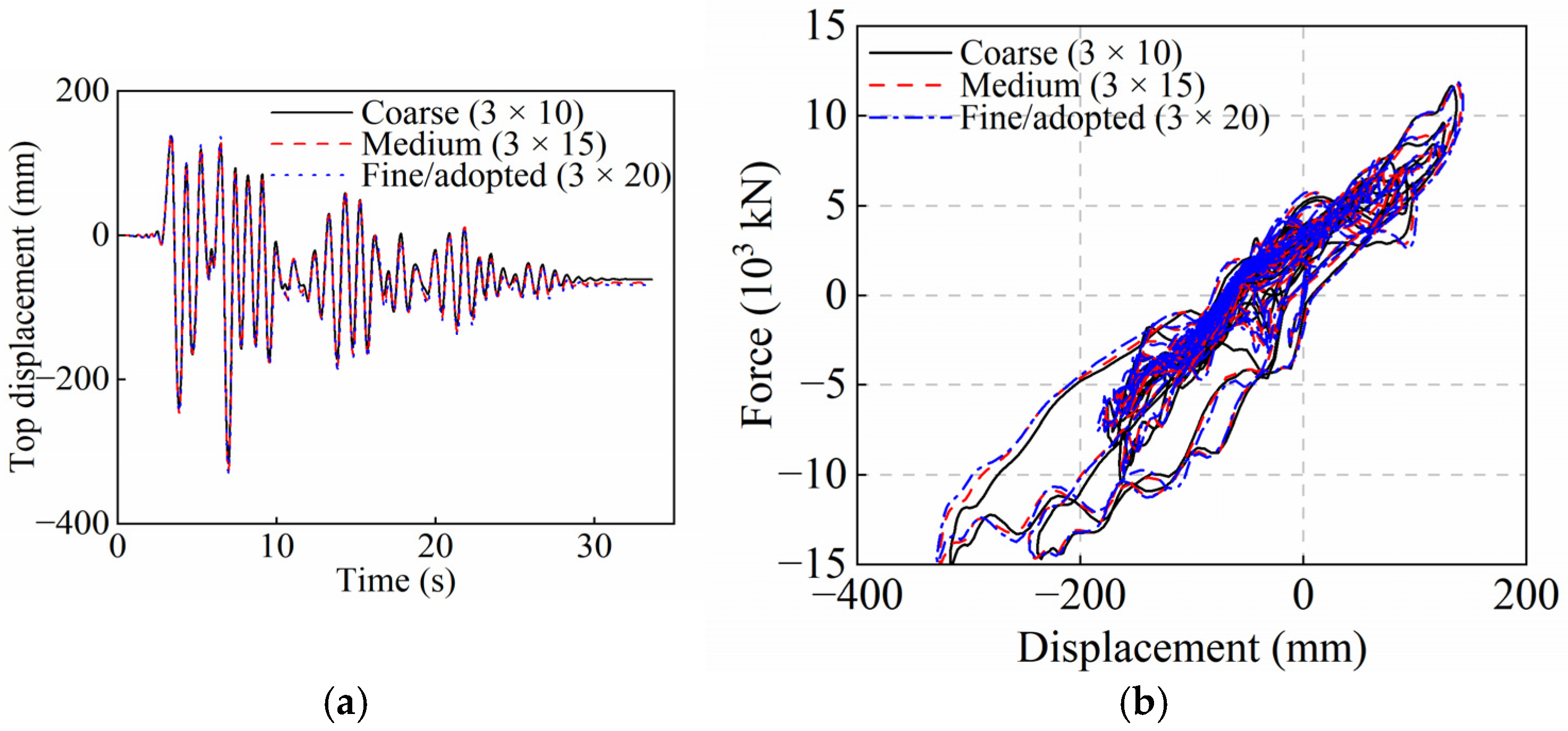
As shown in Figure 15, A complementary dynamic mesh-sensitivity analysis was performed for the 24 m pier under the LP–RSN982 record scaled to PGA = 0.8 g. Both formulations were analyzed using 10, 15, and 20 longitudinal elements, with all non-mesh parameters and the nonlinear solution settings described above held constant. No time-step reduction was required, and all six cases completed the 33.6 s analysis. Relative to the adopted 20-element mesh, the 15-element AFSI–MBTEM model differed by 0.23% in the first period, 0.68% in peak pier-top displacement, and 0.51% in peak element-cut base shear; its displacement time-history nRMSE and dynamic loop-integrated work difference were 0.66% and 1.61%, respectively. The corresponding differences for the flexure model were 0.02%, 0.002%, 0.64%, 0.13%, and 2.38%. These small changes indicate that the adopted discretization is sufficiently stable for the global dynamic response measures examined herein.

5. Seismic Fragility Analysis

5.1. Methodology

Seismic fragility describes the conditional probability that the seismic demand imposed on a structure reaches or exceeds the capacity associated with a prescribed damage state at a given ground-motion intensity [36,37,38]. In the present study, an analytical fragility framework based on nonlinear time-history analysis was adopted to quantify and compare the seismic vulnerability predicted by the flexure model and AFSI–MBTEM. For the $k$th damage state, the fragility function is expressed as:

$$P_{f,k}\left(IM\right)=P[D\ge C_k\mid IM]$$

(3)

where $D$ denotes the seismic demand, $C_k$ is the capacity corresponding to the $k$th damage state, and $IM$ is the selected ground-motion intensity measure. Peak ground acceleration (PGA) was adopted as the IM because it provides a consistent scaling basis for comparing non-pulse and pulse-like ground motions and has been extensively employed in the fragility assessment of bridge piers [39,40,41].

The nonlinear dynamic analysis matrix comprised three independently analyzed pier-level configurations with heights of 16, 24, and 32 m. Each configuration was simulated using both the flexure model and AFSI–MBTEM. Four ground-motion categories were considered, with 20 records in each category. Every record was scaled from 0.1 to 1.5 g at intervals of 0.1 g. Thus, 7200 nonlinear time-history analyses were conducted, enabling controlled comparisons across the two model formulations, three pier configurations, and four ground-motion categories.

Of the 7200 nonlinear time-history analyses, 7183 were completed successfully, corresponding to a completion rate of 99.764%. Numerical nonconvergence occurred in 17 analyses (0.236%). These cases were excluded from the corresponding primary PSDM regressions and were not reassigned as physical collapse observations. No analysis reached the 10% drift-ratio threshold used for numerical collapse screening; therefore, numerical nonconvergence was treated separately from drift-threshold exceedance.

The maximum displacement ductility demand was selected as the engineering demand parameter (EDP):

$${\mu }_d={\displaystyle \frac{{max}_t\left|{\Delta }_{\mathrm{t}\mathrm{o}\mathrm{p}}\right(t\left)\right|}{{\Delta }_y}}$$

(4)

where ${\Delta }_{\mathrm{t}\mathrm{o}\mathrm{p}}\left(t\right)$ is the time-history response of the pier-top displacement, and ${\Delta }_y$ is the common reference yield displacement. The yield displacement was determined by conducting separate pushover analyses of the flexure model and AFSI–MBTEM under the same gravity-induced axial load as that employed in the nonlinear dynamic analyses. The first yielding of the longitudinal reinforcement was adopted as the yield criterion, and the arithmetic mean of the yield displacements predicted by the two models was used as the common value for each pier height. The resulting yield displacements for the 16, 24, and 32 m bridge piers were 0.0551, 0.1238, and 0.2199 m, respectively. The same yield displacement was applied to both models at each height to ensure that differences in displacement ductility reflected differences in the predicted seismic demand rather than model-specific normalization. This common definition also facilitated consistent comparisons among the three height–shear-span configurations.

For each combination of ground-motion category, numerical model, and pier height, the relationship between the median seismic demand and PGA was represented by the conventional power-law probabilistic seismic demand model (PSDM):

$$S_D\left(IM\right)=a(IM{)}^b$$

(5)

where $S_D$ is the median displacement ductility demand and $a$ and $b$ are regression coefficients. Equation (5) can be transformed into a linear relationship in logarithmic space:

$$\mathrm{l}\mathrm{n}{\mu }_{d,i}=\mathrm{l}\mathrm{n}a+b\mathrm{l}\mathrm{n}{\mathrm{P}\mathrm{G}\mathrm{A}}_i+{\epsilon }_i$$

(6)

where ${\epsilon }_i$ is the regression residual, which is assumed to follow a normal distribution with a zero mean and constant variance. All record-level responses were included in the regression rather than first averaging the responses at each PGA level, thereby preserving the record-to-record variability. The logarithmic dispersion of demand was calculated as:

$${\beta }_{D\mid IM}=\sqrt{{\displaystyle \frac{{\sum }_{i=1}^N{[\mathrm{l}\mathrm{n}{\mu }_{d,i}-\mathrm{l}\mathrm{n}(a{\mathrm{P}\mathrm{G}\mathrm{A}}_i^b)]}^2}{N-2}}}$$

(7)

where $N$ is the number of valid nonlinear analyses used for each PSDM. The coefficient of determination, $R^2$, was used to evaluate the adequacy of the log-linear regression. The fitted regression coefficients $a$ and $b$, together with the corresponding $R^2$ values, are presented in Section 5.4. The same regression procedure was applied to all pier configurations, numerical models, and ground-motion groups.

Assuming that both seismic demand and damage-state capacity follow lognormal distributions and are statistically independent, the logarithmic capacity dispersion can be obtained from its coefficient of variation as:

$${\beta }_{C,k}=\sqrt{\mathrm{l}\mathrm{n}(1+{\mathrm{C}\mathrm{O}\mathrm{V}}_{C,k}^2)}$$

(8)

The probability of exceeding the $k$th damage state at a specified PGA can subsequently be expressed as:

$$P_{f,k}(\mathrm{P}\mathrm{G}\mathrm{A})=\Phi [{\displaystyle \frac{\mathrm{l}\mathrm{n}(a{\mathrm{P}\mathrm{G}\mathrm{A}}^b)-\mathrm{l}\mathrm{n}{S}_{C,k}}{\sqrt{{\beta }_{D\mid IM}^2+{\beta }_{C,k}^2}}}]$$

(9)

where $S_{C,k}$ is the median displacement ductility capacity associated with the $k$th damage state, and $\Phi (·)$ is the standard normal cumulative distribution function. The damage-state capacities and their associated uncertainties are defined in Section 5.2.

Equation (9) can alternatively be expressed in the conventional lognormal fragility form:

$$P_{f,k}(\mathrm{P}\mathrm{G}\mathrm{A})=\Phi [{\displaystyle \frac{\mathrm{l}\mathrm{n}(\mathrm{P}\mathrm{G}\mathrm{A}/{\theta }_k)}{{\beta }_{IM,k}}}]$$

(10)

where the median PGA capacity ${\theta }_k$, and the logarithmic dispersion in the IM domain are calculated as:

$${\theta }_k={({\displaystyle \frac{S_{C,k}}{a}})}^{1/b},{\beta }_{IM,k}={\displaystyle \frac{\sqrt{{\beta }_{D\mid IM}^2+{\beta }_{C,k}^2}}{b}}$$

(11)

Separate PSDMs and fragility curves were developed for the flexure model and AFSI–MBTEM. Model identity was therefore treated as a deterministic alternative rather than an additional random variable, and no pooled model-form dispersion was added to Equation (9). This treatment allows the influence of neglecting or explicitly considering axial–flexure–shear interaction to be directly reflected by differences between the two sets of fragility curves. In total, 24 PSDMs were established for the combinations of the two models, three pier heights, and four ground-motion categories. Combining these PSDMs with the four prescribed damage states produced 96 fragility curves.

5.2. Definition of Limit States

The displacement ductility ratio was adopted as a dimensionless damage index to quantify post-yield deformation and enable consistent comparisons across the coupled height–shear-span configurations. Following Buckle et al. [42], four damage states were defined as slight damage (DS1), moderate damage (DS2), severe damage (DS3), and the adopted near-collapse ductility limit (DS4), with median ductility capacities $S_c$ of 1.0, 1.2, 1.76, and 3.0, respectively. In the present study, DS4 denotes exceedance of the adopted near-collapse displacement-ductility limit rather than the simulation of physical bridge collapse. Their physical descriptions were established with reference to the observed damage progression of RC hollow piers [26]. The capacities were assumed to follow lognormal distributions, with coefficients of variation of 0.25 for DS1–DS2 and 0.50 for DS3–DS4 [42], corresponding to logarithmic dispersions ${\mathsf{\beta }}_c$ of 0.246 and 0.472. The adopted limit states are summarized in

Table 4. Definition of limit states for bridge piers.

Limit State	Bridge Operational Functionality	Seismic Damage State	${\mathbf{S}}_{\mathbf{C}}$	${\mathsf{\beta }}_{\mathfrak{c}}$
Slight damage (DS1)	Fully operational	Minor cracking of cover concrete or initial yielding of longitudinal reinforcement	1	0.246
Moderate damage (DS2)	Operational	Initial formation of local plastic hinges, with visible surface cracks	1.2	0.246
Severe damage (DS3)	Life safety	Full formation of plastic hinges, appearance of wide cracks, and extensive spalling of concrete	1.76	0.472
Near-collapse limit (DS4)	Near-collapse condition	Severe strength degradation, extensive yielding of longitudinal reinforcement, and crushing of core concrete	3.0	0.472

.

It should be emphasized that the numerical models do not explicitly simulate loss of axial-load-carrying capacity, global dynamic instability, or complete-bridge collapse. Therefore, the DS4 results are interpreted as probabilities of exceeding the adopted near-collapse ductility limit rather than probabilities of actual physical collapse.

The four limit states are cumulative exceedance states. We let Pk(PGA) denote the probability of exceeding DSk at a given PGA, which gives the expression:

$$P_1\left(PGA\right)\ge P_2\left(PGA\right)\ge P_3\left(PGA\right)\ge P_4\left(PGA\right)$$

(12)

The same damage-state thresholds and capacity uncertainties were applied to both the flexure model and AFSI–MBTEM and to all three pier heights. Consequently, differences between the resulting fragility curves arise from the seismic demands predicted by the two modeling approaches rather than from different definitions of structural capacity. This consistent limit-state framework enables a direct comparison of the two model formulations and ground-motion pulse characteristics across the three coupled height–shear-span configurations.

To relate the generic baseline limits to the observed damage of the tested hollow piers, a test-informed classification was obtained from the same experimental database [26], which included specimens G1–G3, H1–H2, and I1–I2. Based on crack development, reinforcement and concrete strains, strength and stiffness degradation, and residual displacement, the reported displacement-ductility ranges for essentially intact, slight, moderate, severe, and collapse-control performance were 0–0.8, 0.8–1.8, 1.8–3.0, 3.0–4.1, and 4.1–5.0, respectively. Accordingly, the onset values of 0.8, 1.8, 3.0, and 4.1 were adopted as a test-informed alternative set for DS1–DS4 in the sensitivity analysis. The last value is interpreted here as the onset of the adopted near-collapse ductility limit rather than physical collapse.

5.3. Ground-Motion Selection

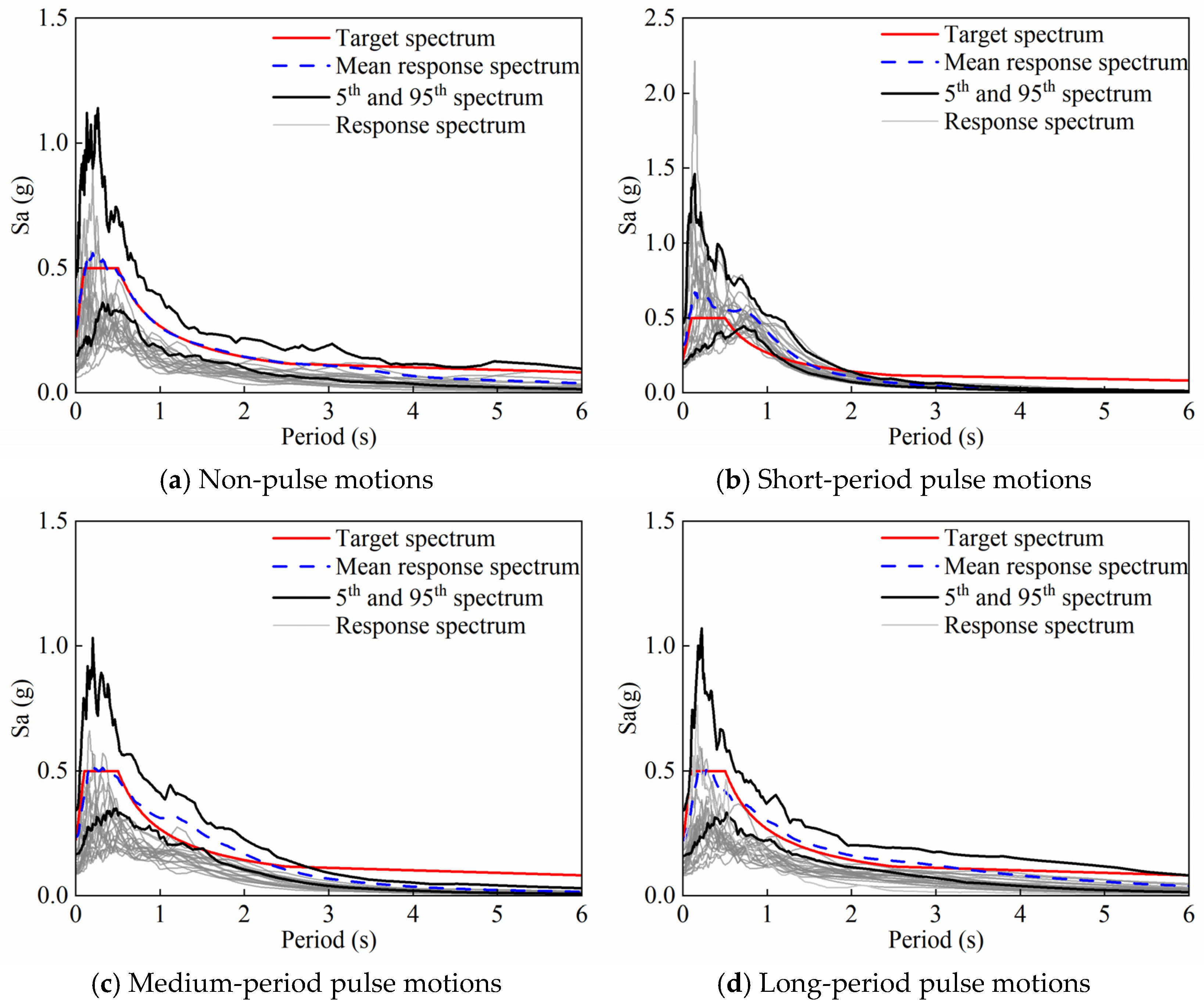
Near-fault ground motions may contain strong velocity pulses that concentrate seismic demand within a limited period range. Bridge response therefore depends not only on ground-motion intensity but also on the relationship between the pulse period and the structural period. To examine this effect, 80 horizontal records were selected from the PEER NGA-West2 database [43] and classified into four groups: non-pulse motions (NP), short-period pulse-like motions (SP), medium-period pulse-like motions (MP), and long-period pulse-like motions (LP), with 20 records in each group. The target design spectrum was defined in accordance with JTG/T 2231-02-2021 and GB 18306-2015 [44,45]. For the adopted site class and seismic hazard level, the site-adjusted design PGA and characteristic period $T_g$ were taken as 0.22 g and 0.50 s, respectively, with a damping ratio of 5%.

Pulse-like motions were identified by the presence of a pronounced velocity pulse characterized by the pulse period $T_p$, following established wavelet-based identification procedures [13]. No dominant velocity pulse was identified for the NP records; therefore, $T_p$ was not assigned to this group. The relative pulse-to-structure period ratio was defined as:

$$R_T={\displaystyle \frac{T_p}{T_1}}$$

(13)

where $T_1$ is the fundamental period of the reference complete-bridge system in Section 4.1. Its mean value was approximately 1.645 s. The pulse-period characteristics of the four ground-motion groups are summarized in

Table 5. Pulse-period characteristics of the selected ground-motion groups.

Ground-Motion Group	Abbreviation	Number of Records	${\mathit{T}}_{\mathit{p}}$ Range (Mean), s	${\mathit{R}}_{\mathit{T}}$ Range (Mean)	Relative-Period Characteristic
Non-pulse motions	NP	20	N/A	N/A	No dominant velocity pulse
Short-period pulse-like motions	SP	20	0.728–1.246 (1.071)	0.443–0.757 (0.651)	Pulse period shorter than $T_1$
Medium-period pulse-like motions	MP	20	1.330–2.436 (1.836)	0.809–1.481 (1.116)	Pulse period close to $T_1$
Long-period pulse-like motions	LP	20	2.570–4.998 (3.929)	1.562–3.038 (2.388)	Pulse period substantially longer than $T_1$

. For the controlled comparison, the relative-period ratio $R_T$ = $T_p/T_1$ was divided into nonoverlapping intervals: SP for $R_T<0.8$, MP for $0.8\le R_T\le 1.5$, and LP for $R_T>1.5$. These thresholds separated pulse periods below, around, and above the bridge-system reference period, while NP records had no identified dominant pulse and served as the baseline.

The complete-bridge period was adopted because the record groups represent longitudinal excitation of the prototype bridge system, whereas the 16, 24, and 32 m pier-level models represent its individual piers using consistent section, axial-load, and tributary-mass assumptions. This common reference preserves identical record groups for the controlled model comparison, but it does not capture possible reclassification based on the isolated period of each pier model. Accordingly, the SP/MP/LP comparisons are interpreted at the bridge-system level; sensitivity to pier-specific reference periods remains a limitation and should be examined in future work.

As summarized in Table 5, the NP group provides a non-pulse baseline, whereas the SP, MP, and LP groups represent pulse periods shorter than, close to, and substantially longer than the common reference period $T_1$ of the complete-bridge system, respectively. The MP group was therefore used to examine possible system-level period-proximity effects. Figure 16 presents the 5% damped acceleration response spectra of the selected records. The gray curves represent individual records, the dashed curves denote the group means, and the black curves indicate the fifth and 95th percentiles. The target design spectrum is also included for comparison. The mean spectra generally follow the target spectrum over the period range of interest while retaining sufficient record-to-record variability.

5.4. Comparative Seismic Fragility Assessment

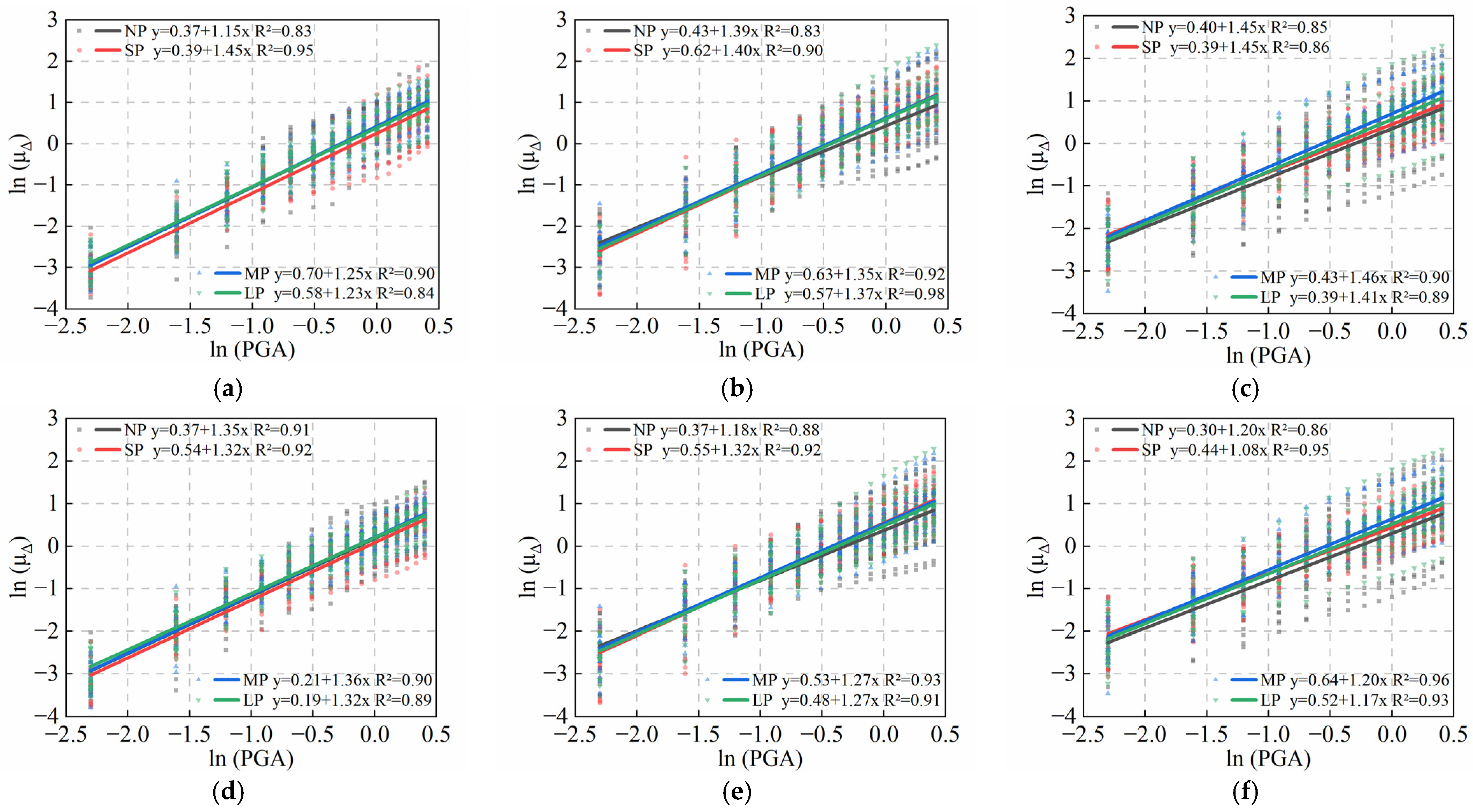
The PSDMs obtained for the three coupled height–shear-span configurations are presented in Figure 17. Power-law regressions were developed separately for the flexure model and AFSI–MBTEM under the NP, SP, MP, and LP ground-motion groups. The fitted log-linear intercept $\ln a$, slope $b$, and coefficient of determination $R^2$ are reported in each panel to facilitate comparison of seismic demand trends and regression quality.

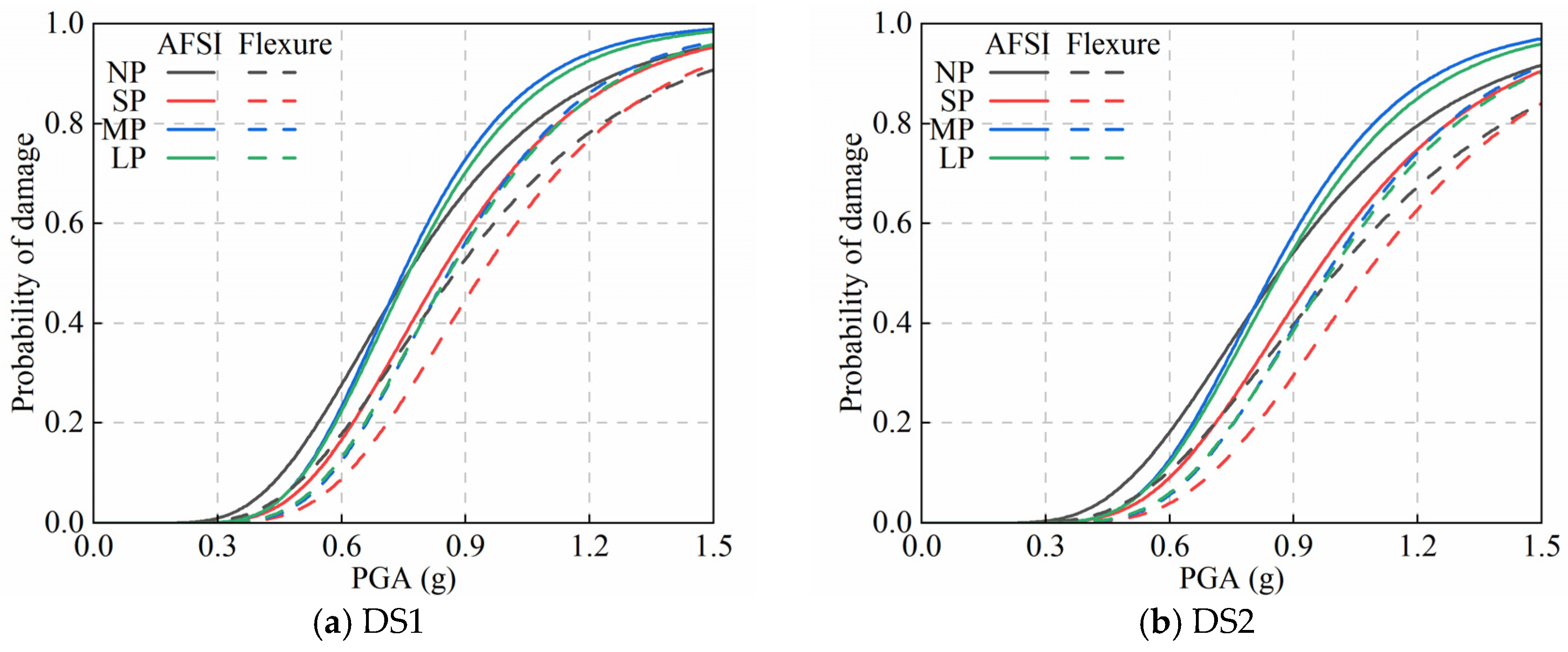
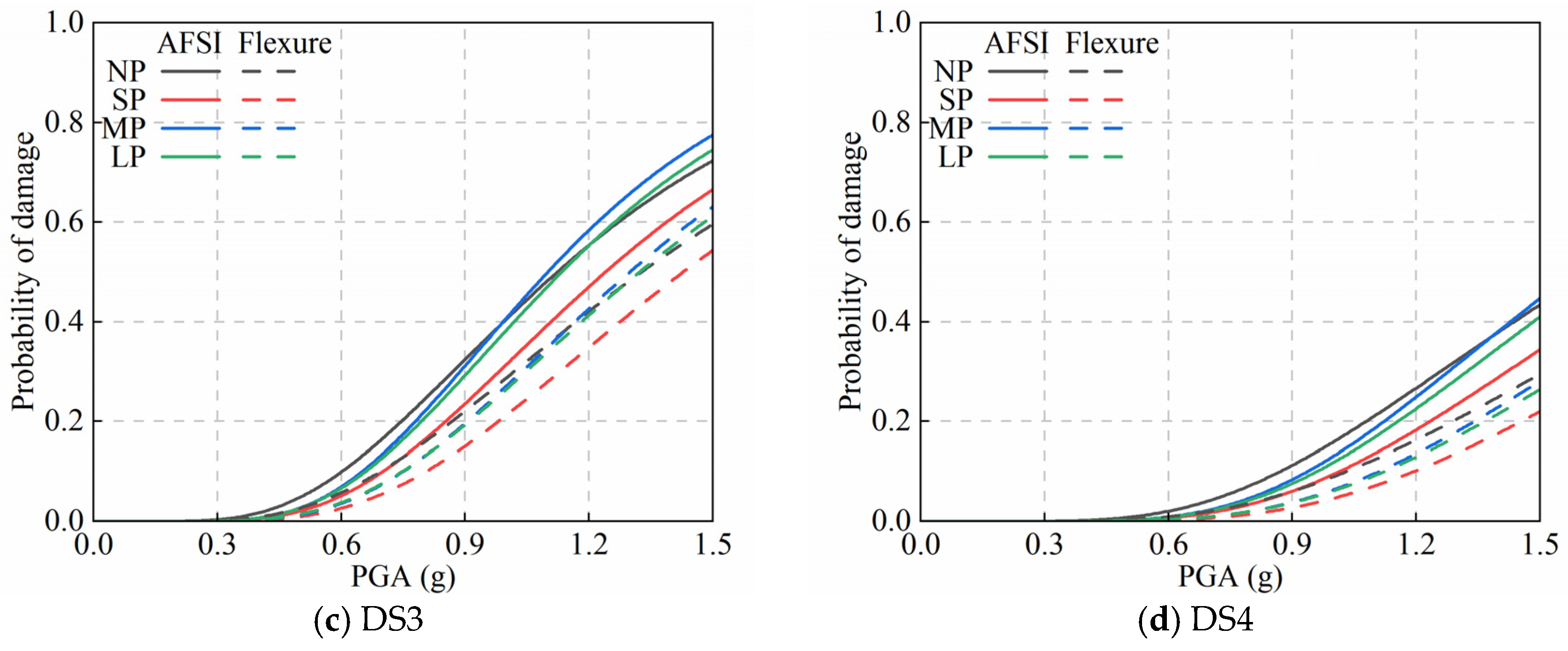
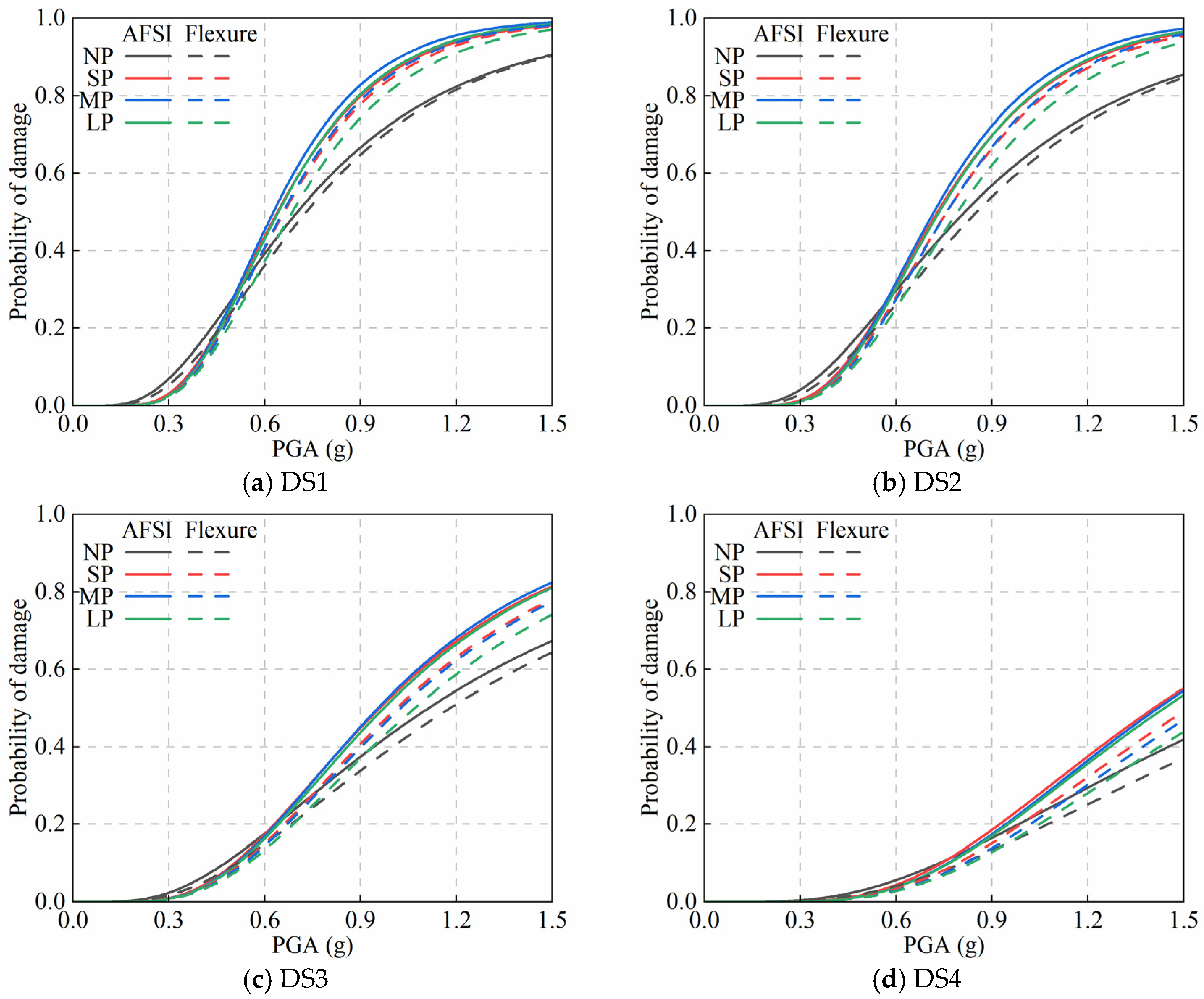
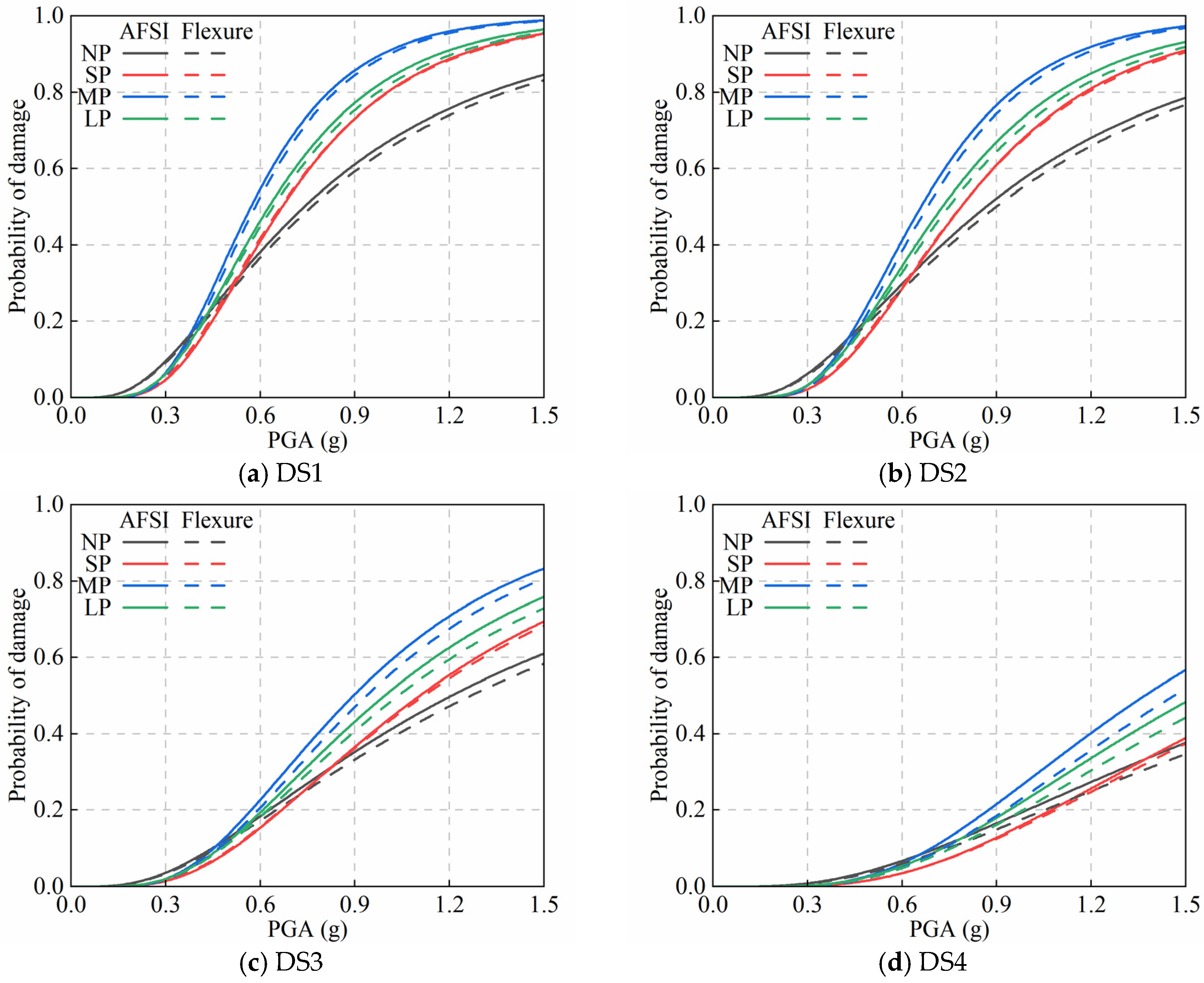
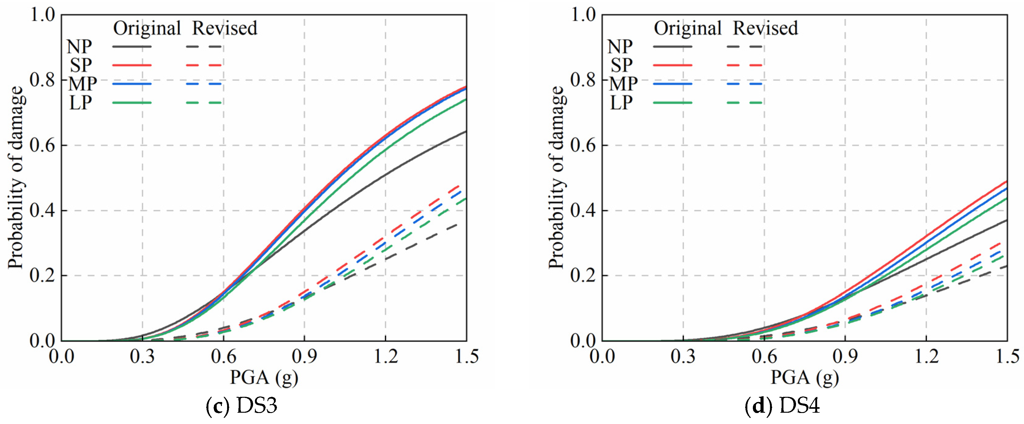
AFSI–MBTEM produced a leftward fragility-curve shift in 46 of the 48 fitted comparisons, indicating generally higher predicted fragility. Because some DS4 median capacities exceeded the analyzed PGA range, DS4 was evaluated using exceedance probabilities at PGA = 1.5 g. The observed differences represent the combined effect of pier height and shear-span ratio.

For the 16 m pier with $\lambda =4$, AFSI–MBTEM reduced the median DS1 capacity by 10.8–13.0%, as shown in Figure 18. Because the fitted DS4 medians exceeded the analyzed range, DS4 was compared at PGA = 1.5 g, where the MP motion exceedance probability increased from 0.281 to 0.447. This result indicates that the shear interaction increased the predicted fragility of the 16 m (λ = 4) coupled configuration.

For the 24 m pier with $\lambda =6$, the influence of axial–flexure–shear interaction remained evident but was weaker than for the 16 m ($\lambda =4$) configuration. As shown in Figure 19, AFSI–MBTEM reduced the median DS1 capacity by 3.1–6.3%. Because some fitted DS4 medians exceeded the analyzed range, DS4 was compared at PGA = 1.5 g. Under LP motions, the DS4 exceedance probability increased from 0.439 to 0.534, indicating that long-period displacement demand enhanced the model-form effect. Overall, the smaller discrepancy relative to the 16 m ($\lambda =4$) configuration indicates weaker shear influence for the coupled 24 m ($\lambda =6$) configuration.

For the 32 m pier with a shear-span ratio of eight, the fragility curves predicted by the two models were generally close, as shown in Figure 20. Under MP motions, the median DS4 capacity decreased from 1.463 to 1.370 g, while the exceedance probability at PGA = 1.5 g increased from 0.518 to 0.568. In contrast, the DS1 and DS2 capacities under SP motions predicted by AFSI–MBTEM were only 0.72% and 0.13% higher than those predicted by the flexure model, respectively. These minor reversals indicate that the corresponding curves were essentially coincident. Thus, the 32 m pier was predominantly flexure-controlled, although the shear interaction still affected its severe-damage response.

The ground-motion category also affected fragility across the three coupled height–shear-span configurations. MP motions generally produced the highest fragility for the 16 m ($\mathsf{\lambda }=4$) configuration, whereas SP and MP motions produced comparable fragilities for the 24 m ($\lambda =6$) configuration. For the 32 m ($\lambda =8$) configuration, MP motions produced the highest DS4 exceedance probability at PGA = 1.5 g, reaching 0.568 for AFSI–MBTEM. Because the MP pulse periods were close to the common first longitudinal period of the complete-bridge system, this result suggests a possible system-level period-proximity effect rather than a tall-pier-specific resonance. Overall, fragility was governed jointly by the coupled height–shear-span configuration and ground-motion pulse characteristics.

Within the analyzed PGA range, the model-form difference was generally more evident for the severe damage states. At PGA = 1.5 g, AFSI–MBTEM predicted higher DS4 exceedance probabilities for the critical cases of all three pier configurations. This result indicates that neglecting the shear interaction may underestimate the probability of exceeding the adopted DS4 near-collapse ductility limit, particularly for configurations with greater shear participation and motions producing large inelastic displacement demands.

5.5. Sensitivity to Damage-State Thresholds

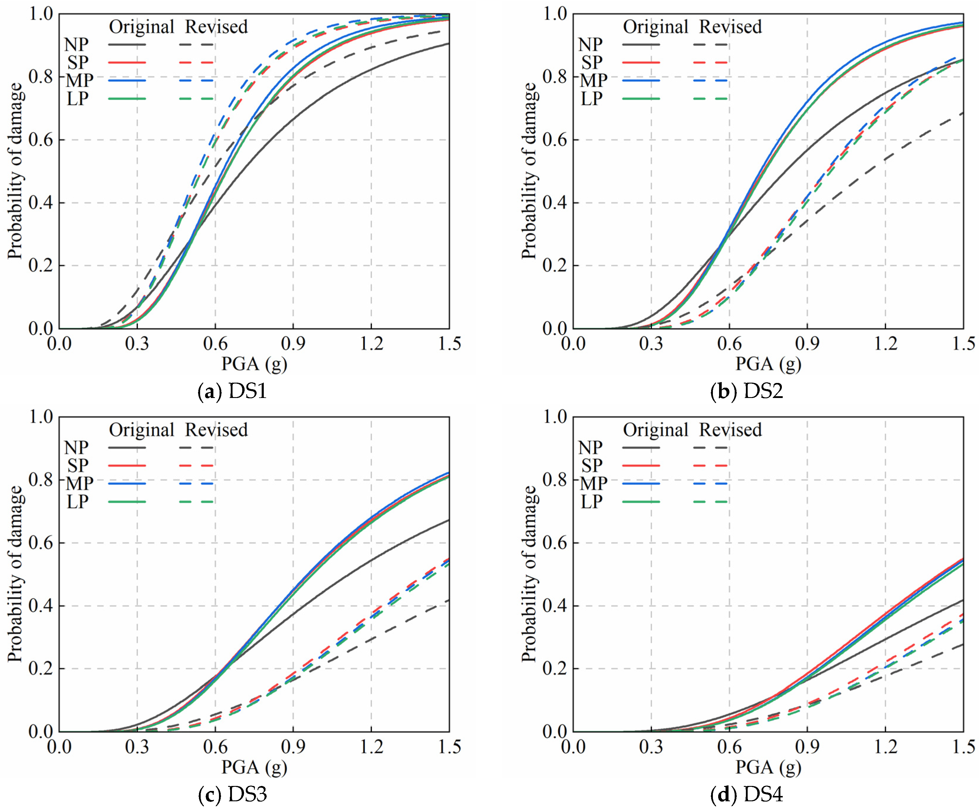
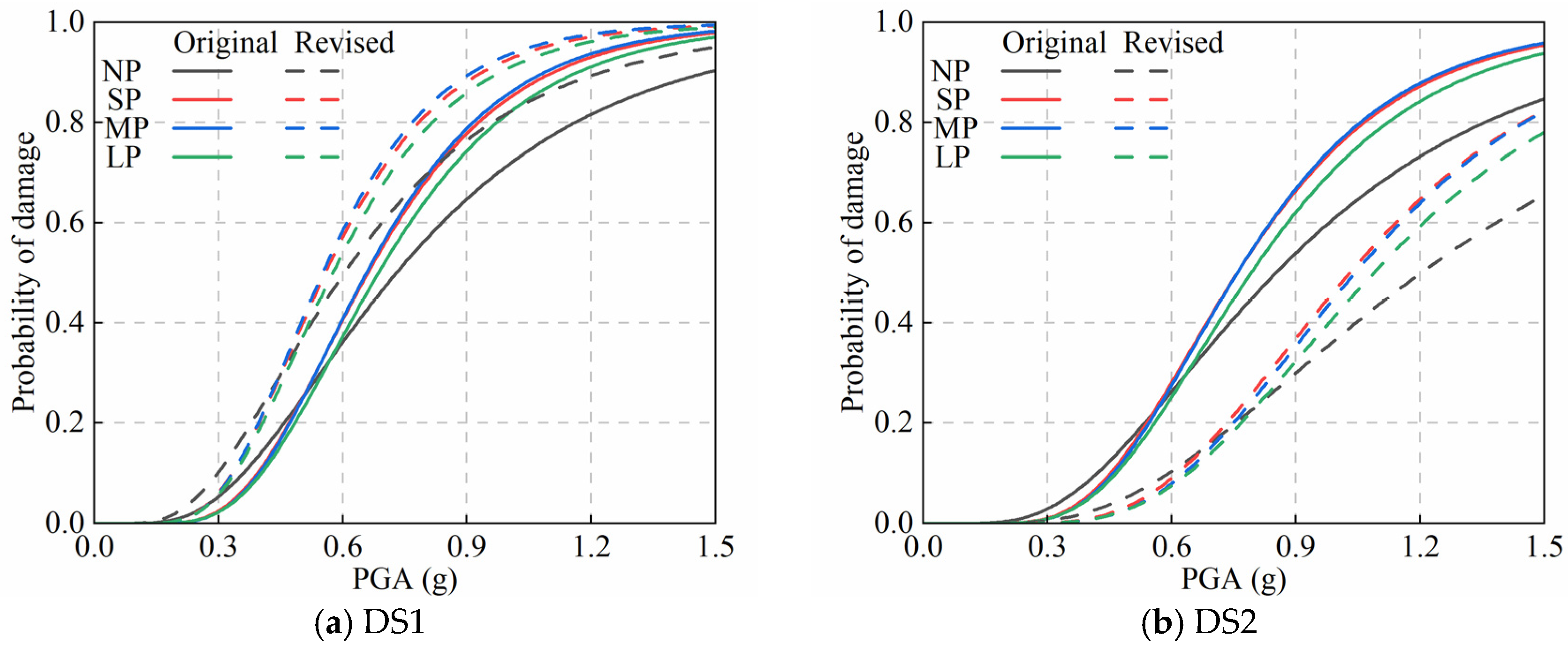
To assess whether the model-form comparison depended on the generic baseline limits, a representative threshold-sensitivity analysis was conducted for the 24 m pier (λ = 6), which represents the intermediate coupled height–shear-span configuration. The eight existing PSDMs for the two model formulations and four ground-motion groups were retained, together with the adopted capacity dispersions. Only the median ductility thresholds were changed from [1.0, 1.2, 1.76, 3.0] to [0.8, 1.8, 3.0, 4.1], thereby isolating the effect of limit-state selection without rerunning the nonlinear time-history analyses. Figure 21 and Figure 22 compare the resulting curves for AFSI–MBTEM and the flexure model, respectively; solid and dashed lines denote the baseline and test-informed limits.

As expected, reducing the DS1 threshold from 1.0 to 0.8 shifted the corresponding curves to the left and lowered the fitted median PGA capacities by 14.8–17.3%. Increasing the DS2 threshold from 1.2 to 1.8 shifted the curves to the right and raised the fitted median capacities by 33.7–41.1%. Because some fitted DS3 and DS4 medians exceeded the analyzed upper limit of 1.5 g, their sensitivity was evaluated using in-range exceedance probabilities at PGA = 1.5 g. The test-informed limits reduced the DS3 and DS4 exceedance probabilities by 25.5–30.5 and 14.1–18.8 percentage points, respectively. Thus, the absolute fragility estimates were sensitive to the selected ductility thresholds, particularly for the more severe damage states.

Nevertheless, the principal model-form comparison remained stable. Under the test-informed thresholds, AFSI–MBTEM yielded lower fitted median PGA capacities than the flexure model for all 16 ground-motion group and damage-state combinations. At PGA = 1.5 g, its DS2–DS4 exceedance probabilities were 3.1–9.5 percentage points higher, whereas the DS1 difference remained within 0.55 percentage points. The sensitivity analysis therefore confirms that threshold selection affects the absolute fragility level but does not alter the main conclusion that explicit axial–flexure–shear interactions generally predict higher fragility for the representative 24 m configuration.

6. Conclusions

This study investigated the seismic behavior and fragility of rectangular RC hollow bridge piers by integrating cyclic loading tests, numerical model validation, full-scale pier analyses, and nonlinear seismic fragility assessment. Particular attention was given to the influence of axial–flexure–shear interaction and its variation across the three coupled height–shear-span configurations and near-fault ground-motion categories. Based on the results obtained in this study, the following conclusions can be drawn.

(1)

The seven rectangular hollow-pier specimens exhibited flexure-dominated but distinctly shear-sensitive failure behavior. Flexural cracking initiated the nonlinear response, whereas inclined cracking, shear deformation, concrete deterioration, and reinforcement instability became increasingly important after yielding. Reducing the shear-span ratio substantially increased lateral resistance but intensified crack localization and post-peak deterioration. Increasing the transverse reinforcement ratio improved cyclic stability and restrained diagonal-crack development. In contrast, increasing the longitudinal reinforcement ratio from 1.63% to 2.15% markedly increased the peak resistance, whereas a further increase to 2.69% produced little additional strength improvement, indicating that the contribution of longitudinal reinforcement became limited by shear-related damage and concrete deterioration.

(2)

Both numerical formulations reproduced the overall lateral resistance and hysteretic response of the test specimens, but their accuracy depended on the relative contribution of shear deformation. The flexure model generally produced wider hysteretic loops and overestimated the energy dissipation of shear-sensitive specimens. By explicitly representing the axial–flexure–shear interaction, AFSI–MBTEM provided closer predictions of pinching, unloading and reloading paths, post-peak deterioration, effective stiffness, and hysteretic energy. For the complete specimen set, the mean absolute error in hysteretic energy decreased from 23.57% for the flexure model to 13.29% for AFSI–MBTEM. The improvement was particularly evident for G1, for which the hysteretic energy error decreased from approximately 40.8% to 5.1%. Across the investigated specimens, the two models produced increasingly similar predictions as the shear-span ratio increased, indicating that the advantage of AFSI–MBTEM was most pronounced for G1 and the other cases with greater observed shear participation.

(3)

Under cyclic loading, AFSI–MBTEM reduced the peak strengths of the 16, 24, and 32 m piers by 5.54%, 4.56%, and 1.26%, respectively. At the common drift ratio of 5.5%, it also produced higher second-to-first-cycle strength-retention ratios, indicating improved repeated-cycle stability with large deformation. However, the change in cumulative hysteretic energy was not monotonic across the three configurations.

(4)

Under the representative near-fault ground motions, the influence of axial–flexure–shear interaction depended jointly on the coupled height–shear-span configurations and their excitation. For the 16 m pier, AFSI–MBTEM reduced the peak base shear by 8.9–32.8%, while the peak displacement change ranged from −1.9% to 34.7%. For the 24 m pier, the peak displacement increased by 11.0–18.0%, whereas the base-shear change ranged from −4.5% to 12.7%. The two models generally converged for the 32 m pier, except under the MP record, for which AFSI–MBTEM increased the peak displacement and base shear by 21.7% and 11.8%, respectively. Thus, the model effect cannot be represented by a single correction factor.

(5)

Explicit consideration of axial–flexure–shear interaction generally increased the predicted seismic fragility, with the AFSI–MBTEM curves shifted to the left in 46 of the 48 fitted comparisons. At PGA = 1.5 g, the DS4 exceedance probability increased from 0.281 to 0.447 for the 16 m configuration under MP motions, from 0.439 to 0.534 for the 24 m configuration under LP motions, and from 0.518 to 0.568 for the 32 m configuration under MP motions. These in-range results indicate that neglecting the shear interaction may produce nonconservative fragility estimates, particularly for severe damage states and configurations with greater shear participation. For the representative 24 m configuration, the same model ranking was retained under the test-informed ductility limits, confirming that the principal model-form conclusion was not an artifact of the original thresholds.

Overall, the results demonstrate that the seismic response of rectangular RC hollow bridge piers is governed by the interactions between flexural yielding, shear deformation, cyclic deterioration, pier geometry, and ground-motion frequency content. A flexure-only model may be adequate for estimating some response quantities of slender piers, but AFSI–MBTEM provides a more mechanically consistent basis for predicting hysteretic behavior, cumulative damage, and seismic fragility. These conclusions are limited to the investigated rectangular hollow-section geometry, fixed wall thickness, reinforcement ranges, axial-load ratio of 0.05, longitudinal loading direction, coupled height–shear-span configurations, and selected ground-motion sets. They should not be generalized to other rectangular hollow bridge piers without further validation. Future studies should consider different section geometries, wall thicknesses, axial-load ratios, reinforcement arrangements, bidirectional excitations, soil–foundation interactions, and additional experimental validations under near-fault pulse-like ground motions.

References

1. Shao, C.; Qi, Q.; Wang, M.; Xiao, Z.; Wei, W.; Hu, C.; Xiao, L. Experimental Study on the Seismic Performance of Round-Ended Hollow Piers. Eng. Struct. 2019, 195, 309–323. [Google Scholar] [CrossRef] [Scilit]
2. Cassese, P.; Ricci, P.; Verderame, G.M. Experimental Study on the Seismic Performance of Existing Reinforced Concrete Bridge Piers with Hollow Rectangular Section. Eng. Struct. 2017, 144, 88–106. [Google Scholar] [CrossRef] [Scilit]
3. Cui, H.; Shao, C.; Wei, W.; Zhang, Y.; Qi, Q.; Wang, C.; Long, J. Failure Mechanisms and Seismic Damage Control of Variable-Section Round-Ended Hollow Railway Piers in the Transverse Direction. Eng. Fail. Anal. 2026, 193, 110883. [Google Scholar] [CrossRef] [Scilit]
4. Cui, H.; Shao, C. Experimental Study on Seismic Performance of Circular Hollow Piers with Low-to-Medium Shear-Span Ratio in High-Seismic Intensity Regions. Structures 2026, 87, 111767. [Google Scholar] [CrossRef] [Scilit]
5. Cui, H.; Shao, C. Experimental Investigation on the Flexure-Shear Coupled Deformation Performance of Circular Hollow Piers in Highway Bridges. Structures 2026, 88, 111799. [Google Scholar] [CrossRef] [Scilit]
6. Shao, C.; Wei, W.; Wu, S.; Qi, Q.; Wang, C. Experimental Investigation on Plastic Hinge Length of RC Round-Ended Hollow Columns with a Variable Section. Eng. Struct. 2023, 290, 116358. [Google Scholar] [CrossRef] [Scilit]
7. Cui, H.; Shao, C.; Wei, W.; Zhang, Y.; Qi, Q.; Long, J. Prediction of Equivalent Damping Ratio for Round-Ended Hollow Railway Bridge Piers with Variable Sections Based on GA-BP Neural Network and Quasi-Static Test. Mech. Syst. Signal Process. 2026, 244, 113810. [Google Scholar] [CrossRef] [Scilit]
8. Cui, H.; Shao, C.; Wei, W.; Zhang, Y.; Qi, Q.; Wang, C. Data-Driven Prediction of Effective Stiffness for Thin-Walled Hollow Piers via a GA-BP Neural Network with Quasi-Static Test Validation. Adv. Eng. Softw. 2026, 218, 104194. [Google Scholar] [CrossRef] [Scilit]
9. Hu, S.; Liao, Y.; Zeng, S.; Sun, Z.; Peng, X. Seismic Retrofitting of Existing Reinforced Concrete Frames Using Eccentric Steel Braces: Experimental Evaluation and Numerical Simulation. Structures 2026, 88, 111824. [Google Scholar] [CrossRef] [Scilit]
10. Qi, Q.; Jiang, L.; Shao, C.; Yang, H.; Shao, J.; Zhou, Y.; Cui, H. Hysteretic Behavior Modeling of RC Walls Considering Axial-Flexure-Shear Interaction. J. Build. Eng. 2025, 111, 113628. [Google Scholar] [CrossRef] [Scilit]
11. Qi, Q.; Shao, C.; Yang, H.; Cui, H.; Chen, Z.; Gong, W. Axial-Flexure-Shear Model for Seismic Analysis of RC Thin-Walled Hollow Piers. Soil Dyn. Earthq. Eng. 2025, 195, 109375. [Google Scholar] [CrossRef] [Scilit]
12. Pan, Z.; Qi, Q.; Duan, L.; Yang, H.; Shao, C.; Li, J.; Cui, H. Parametric Analysis of Reinforced Concrete Hollow Piers Based on an Axial–Flexure–Shear Model Under Cyclic Loading and Earthquake Conditions. Symmetry 2025, 17, 1553. [Google Scholar] [CrossRef] [Scilit]
13. Baker, J.W. Quantitative Classification of Near-Fault Ground Motions Using Wavelet Analysis. Bull. Seismol. Soc. Am. 2007, 97, 1486–1501. [Google Scholar] [CrossRef] [Scilit]
14. Shahi, S.K.; Baker, J.W. An Efficient Algorithm to Identify Strong-Velocity Pulses in Multicomponent Ground Motions. Bull. Seismol. Soc. Am. 2014, 104, 2456–2466. [Google Scholar] [CrossRef] [Scilit]
15. Wan, H.-P.; Su, L.; Frangopol, D.M.; Chang, Z.; Ren, W.-X.; Ling, X. Seismic Response of a Bridge Crossing a Canyon to Near-Fault Acceleration-Pulse Ground Motions. J. Bridge Eng. 2021, 26, 05021006. [Google Scholar] [CrossRef] [Scilit]
16. Yang, T.; Wei, Y.; Zhong, J. Potential Bias of Conventional Structural Seismic Fragility for Bridge Structures under Pulse-like Ground Motions: Bias Evaluation and Strategy Improvement. Soil Dyn. Earthq. Eng. 2023, 166, 107787. [Google Scholar] [CrossRef] [Scilit]
17. Srivastava, C.; Pandikkadavath, M.S.; Mangalathu, S.; AlHamaydeh, M. Seismic Response of RC Bridges under Near-Fault Ground Motions: A Parametric Investigation. Structures 2024, 61, 106033. [Google Scholar] [CrossRef] [Scilit]
18. Jiang, L.; Duan, H.; Wen, T.; Jiang, L. Effects of Near-Fault Pulse-Like Ground Motions and Pulse Parameters on a High-Speed Railway Long-Span Arch Bridge–Track System. J. Bridge Eng. 2025, 30, 04024112. [Google Scholar] [CrossRef] [Scilit]
19. Qi, Q.; Zhou, H.; Yang, H.; Chen, X.; Chen, L.; Shao, C.; Cui, H. Seismic Responses of an FPB-Isolated Railway Continuous Beam Bridge under Pulse-Type Motions: Shaking Table Tests and Simulations. Soil Dyn. Earthq. Eng. 2026, 209, 110506. [Google Scholar] [CrossRef] [Scilit]
20. Polimeru, V.K.; Laskar, A. CSMM Based Seismic Fragility Analysis of Shear Dominant RC Hollow Rectangular Bridge Piers. Bull. Earthq. Eng. 2021, 19, 5051–5085. [Google Scholar] [CrossRef] [Scilit]
21. Duan, L.; Yang, H.; Qi, Q.; Wu, Q.; Shao, C.; Jiang, L. Seismic Fragility of Urban Rail Transport RC Solid Piers Considering Multiparameter Effects. Buildings 2026, 16, 2327. [Google Scholar] [CrossRef] [Scilit]
22. Rahmat Rabi, R.; Monti, G. Machine Learning-Derived Equations for Seismic Fragility of Hollow-Core Bridge Piers Using Analytical Models and Visible Parameters. Structures 2025, 75, 108792. [Google Scholar] [CrossRef] [Scilit]
23. Turchetti, F.; Tubaldi, E.; Douglas, J.; Zanini, M.A.; Dall’Asta, A. A Risk-Targeted Approach for the Seismic Design of Bridge Piers. Bull. Earthq. Eng. 2023, 21, 4923–4950. [Google Scholar] [CrossRef] [Scilit]
24. Homaei, F. The Probabilistic Performance-Based Seismic Assessment of Concrete Bridge Piers with SMASC Reinforcing Bars: Effect of Pulse-like Ground Motion and Vertical Load-to-Capacity Ratio. Soil Dyn. Earthq. Eng. 2024, 185, 108874. [Google Scholar] [CrossRef] [Scilit]
25. Miano, A.; Iacovazzo, P.; Mele, A.; Di Ludovico, M.; Prota, A. Seismic Fragility of Circular Piers in Simply Supported RC Bridges: A Proposal for Capacity Assessment. Eng. Struct. 2024, 302, 117426. [Google Scholar] [CrossRef] [Scilit]
26. Qi, Q.; Shao, C.; Hu, C.; Wei, W.; Xiao, Z. Study on seismic damage assessment and performance level quantification of hollow piers. China Civ. Eng. J. 2020, 53, 116–128. (In Chinese) [Google Scholar]
27. McKenna, F. OpenSees: A Framework for Earthquake Engineering Simulation. Comput. Sci. Eng. 2011, 13, 58–66. [Google Scholar] [CrossRef] [Scilit]
28. Spacone, E.; Filippou, F.C.; Taucer, F.F. Fibre Beam–Column Model for Non-Linear Analysis of R/C Frames: Part I. Formulation. Earthq. Eng. Struct. Dyn. 1996, 25, 711–725. [Google Scholar] [CrossRef] [Scilit]
29. Kent, D.C.; Park, R. Flexural Members with Confined Concrete. J. Struct. Div. 1971, 97, 1969–1990. [Google Scholar] [CrossRef] [Scilit]
30. Karsan, I.D.; Jirsa, J.O. Behavior of Concrete Under Compressive Loadings. J. Struct. Div. 1969, 95, 2543–2564. [Google Scholar] [CrossRef] [Scilit]
31. Mander, J.B.; Priestley, M.J.N.; Park, R. Theoretical Stress-Strain Model for Confined Concrete. J. Struct. Eng. 1988, 114, 1804–1826. [Google Scholar] [CrossRef] [Scilit]
32. Kunnath, S.K.; Heo, Y.; Mohle, J.F. Nonlinear Uniaxial Material Model for Reinforcing Steel Bars. J. Struct. Eng. 2009, 135, 335–343. [Google Scholar] [CrossRef] [Scilit]
33. Vecchio, F.J.; Collins, M.P. The Modified Compression-Field Theory for Reinforced Concrete Elements Subjected to Shear. ACI J. Proc. 1986, 83, 219–231. [Google Scholar] [CrossRef] [Scilit]
34. Hsu, T.T.C.; Zhu, R.R.H. Softened Membrane Model for Reinforced Concrete Elements in Shear. ACI Struct. J. 2002, 99, 460–469. [Google Scholar] [CrossRef] [Scilit]
35. Duan, L.; Yang, H.; Qi, Q.; Wu, Q.; Shao, C.; Yang, Y. Flexure–Shear Response of a RC Double-Column Bridge Pier: Individual Column Cyclic Tests and System-Level Numerical Analysis. Buildings 2026, 16, 3188. [Google Scholar] [CrossRef] [Scilit]
36. Vamvatsikos, D.; Cornell, C.A. Incremental Dynamic Analysis. Earthq. Eng. Struct. Dyn. 2001, 31, 491–514. [Google Scholar] [CrossRef] [Scilit]
37. Cornell, C.A.; Jalayer, F.; Hamburger, R.O.; Foutch, D.A. Probabilistic Basis for 2000 SAC Federal Emergency Management Agency Steel Moment Frame Guidelines. J. Struct. Eng. 2002, 128, 526–533. [Google Scholar] [CrossRef] [Scilit]
38. Baker, J.W. Efficient Analytical Fragility Function Fitting Using Dynamic Structural Analysis. Earthq. Spectra 2015, 31, 579–599. [Google Scholar] [CrossRef] [Scilit]
39. Afsar Dizaj, E.; Salami, M.R.; Kashani, M.M. Nonlinear Dynamic Behaviour and Seismic Fragility Analysis of Irregular Multi-Span RC Bridges. Structures 2022, 44, 1730–1750. [Google Scholar] [CrossRef] [Scilit]
40. Wei, W.; Yuan, Y.; Igarashi, A.; Zhu, H.; Tan, P. Experimental Investigation and Seismic Fragility Analysis of Isolated Highway Bridges Considering the Coupled Effects of Pier Height and Elastomeric Bearings. Eng. Struct. 2021, 233, 111926. [Google Scholar] [CrossRef] [Scilit]
41. Wang, X.; Li, W.; Liu, Z. Experimental Investigation and Fragility Analysis on Seismic Performance of Precast UHPC Hollow Piers under Varying Axial Load. Soil Dyn. Earthq. Eng. 2025, 196, 109420. [Google Scholar] [CrossRef] [Scilit]
42. Buckle, I.; Friedland, I.; Mander, J.; Martin, G.; Nutt, R.; Power, M. Seismic Retrofitting Manual for Highway Structures: Part 1—Bridges; FHWA-HRT-06-032; Federal Highway Administration, Office of Infrastructure Research and Development: McLean, VA, USA, 2006. [Google Scholar]
43. Ancheta, T.D.; Darragh, R.B.; Stewart, J.P.; Seyhan, E.; Silva, W.J.; Chiou, B.S.-J.; Wooddell, K.E.; Graves, R.W.; Kottke, A.R.; Boore, D.M.; et al. NGA-West2 Database. Earthq. Spectra 2014, 30, 989–1005. [Google Scholar] [CrossRef] [Scilit]
44. JTG/T 2231-02-2021; Guidelines for Aseismic Performance Evaluation of Highway Bridges. Ministry of Transport of the People’s Republic of China: Beijing, China, 2021. (In Chinese)
45. GB 18306-2015; Seismic Ground Motion Parameter Zonation Map of China. China Earthquake Administration: Beijing, China, 2015. (In Chinese)
Figure 1. Prototype bridge and geometric details of the full-scale pier and scaled specimens: (a) prototype bridge and full-scale pier cross-section; (b) experimental specimen.
Symmetry 18 01421 g001
Figure 2. Test setup and on-site experimental arrangement.
Symmetry 18 01421 g002
Figure 3. Schematic representation of the hybrid force–displacement cyclic loading protocol.
Symmetry 18 01421 g003
Figure 4. Representative damage evolution and terminal failure of the rectangular hollow-pier specimens.
Symmetry 18 01421 g004
Figure 5. Final crack distributions of specimens G1–G3.
Symmetry 18 01421 g005
Figure 6. Experimental lateral force–displacement hysteretic responses of the rectangular RC hollow-pier specimens.
Symmetry 18 01421 g006
Figure 7. Comparison of the experimental skeleton curves for specimens G1–G3, H1–H2, and I1–I2.
Symmetry 18 01421 g007
Figure 8. Modeling strategies for a rectangular hollow pier: (a) flexure modeling strategy and material constitutive models; (b) AFSI–MBTEM modeling strategy.
Symmetry 18 01421 g008
Figure 9. Comparison of the experimental and numerical hysteretic responses: (a) G1; (b) G2; (c) G3; (d) H1; (e) H2; (f) I1; and (g) I2.
Symmetry 18 01421 g009
Figure 10. Comparison of the computed and experimental response indices for the flexure model and AFSI–MBTEM: (a) yield displacement; (b) yield strength; (c) peak strength; (d) effective stiffness; (e) representative residual displacement; and (f) representative mean single-cycle hysteretic energy.
Symmetry 18 01421 g010
Figure 11. Comparison of the cyclic hysteretic responses predicted by the flexure model and AFSI–MBTEM: (a) H = 16 m and λ = 4; (b) H = 24 m and λ = 6; and (c) H = 32 m and λ = 8.
Symmetry 18 01421 g011
Figure 12. Static mesh-sensitivity comparison for the 24 m AFSI–MBTEM pier under cyclic loading using the 3 × 10, 3 × 15, and 3 × 20 membrane meshes.
Symmetry 18 01421 g012
Figure 13. Four representative ground motions scaled to PGA = 0.8 g: (a) 5% damped acceleration response spectra and (b) acceleration time histories.
Symmetry 18 01421 g013
Figure 14. Base-shear–pier-top displacement responses predicted by the flexure model and AFSI–MBTEM under the representative ground motions: (ac) NP; (df) SP; (gi) MP; and (jl) LP.
Symmetry 18 01421 g014aSymmetry 18 01421 g014b
Figure 15. Dynamic mesh-sensitivity comparison for the 24 m pier under LP–RSN982 scaled to PGA = 0.8 g: (a) pier-top displacement histories and (b) element-cut base-shear–displacement responses.
Symmetry 18 01421 g015
Figure 16. Acceleration response spectra of the selected ground-motion sets: (a) NP; (b) SP; (c) MP; and (d) LP.
Symmetry 18 01421 g016
Figure 17. PSDMs for the 16, 24, and 32 m piers under the four ground-motion groups: (ac) AFSI–MBTEM; (df) flexure.
Symmetry 18 01421 g017
Figure 18. Comparison of the seismic fragility curves predicted by the flexure model and AFSI–MBTEM for the 16 m pier with a shear-span ratio of four: (a) DS1; (b) DS2; (c) DS3; and (d) DS4.
Symmetry 18 01421 g018aSymmetry 18 01421 g018b
Figure 19. Comparison of the seismic fragility curves predicted by the flexure model and AFSI–MBTEM for the 24 m pier with a shear-span ratio of six: (a) DS1; (b) DS2; (c) DS3; and (d) DS4.
Symmetry 18 01421 g019
Figure 20. Comparison of the seismic fragility curves predicted by the flexure model and AFSI–MBTEM for the 32 m pier with a shear-span ratio of eight: (a) DS1; (b) DS2; (c) DS3; and (d) DS4.
Symmetry 18 01421 g020
Figure 21. Sensitivity of the AFSI–MBTEM fragility curves for the 24 m pier to the damage-state thresholds: (a) DS1; (b) DS2; (c) DS3; and (d) DS4. Solid and dashed lines denote the baseline and test-informed thresholds, respectively.
Symmetry 18 01421 g021
Figure 22. Sensitivity of the flexure model fragility curves for the 24 m pier to the damage-state thresholds: (a) DS1; (b) DS2; (c) DS3; and (d) DS4. Solid and dashed lines denote the baseline and test-informed thresholds, respectively.
Symmetry 18 01421 g022aSymmetry 18 01421 g022b