A Novel Model for Solving Mixed Integral Equations with Generalized Kernels

Abstract

This research focuses on the relationship between position and time. A first-order integro-partial differential equation in time and the nth dimension of position is considered in the space $L_2\left(\Omega \right)\times C[0,T],T<1$, where $\Omega$ denotes the domain of integration with respect to position. The position-specific kernel is assumed to be a singular kernel from which many important kernels with physical and geometric significance can be derived, such as Carleman-, Cauchy-, logarithmic-, and Hilbert-type kernels. The time-specific kernel is assumed to be continuous. The integro-differential equation is transformed into a mixed equation, and many important special cases are derived, some of which have not been previously presented. Moreover, under certain assumptions, the existence and uniqueness properties of the proposed equation are studied, as well as convergence and relative errors. The variables are separated to yield a Fredholm integral equation of the second kind with a singular kernel and time-varying coefficients. As the potential kernel is in a general singular state, the Toeplitz matrix method—which is considered the best approach for solving singular integral equations as it can convert singular integrals into calculable ordinary integrals—is used to solve the Fredholm integral equation to obtain and study a linear algebraic system. Finally, for applications assuming special types of kernels, the numerical solutions and their related errors are calculated for each case. Solved cases show how strong, efficient, and straightforward the proposed method is. The results of this investigation show that the method converges quickly for all kernel types.

1. Introduction

Integro-differential equations (I-DEs) are used to simulate various phenomena in the fundamental sciences; for example, the authors of [1] studied the nonlinear response of a cantilever subjected to a first parametric stimulation, which led to the formulation of two I-DEs. I-DEs have been essential in discovering solutions to more complex problems, consistent with the rapid progress made in addressing a range of challenges arising in fundamental scientific research. The Atangana–Baleanu, Caputo, and Caputo–Fabrizio fractional operators were used to formulate I-DE models of plasma dilution in [2]; meanwhile, in [3], an I-DE utilizing a single prognostic variable was developed for the modeling of COVID-19 epidemic dynamics.

At present, many scientists are focusing on developing methods to solve I-DEs. Analytically, the Schauder fixed-point theorem and Banach’s fixed-point theorem were used for this purpose in [4]. Theoretical conclusions resulting from the idea of graphically representing contractions were used to investigate the existence of solutions for nonlinear Volterra–Fredholm integral equations (V-FIEs) and fractional differential equations [5].

When analytical answers are difficult to obtain, some authors focus on numerical solutions. A partial integro-differential equation (I-PDE) was numerically solved using the fourth-order finite-difference and collocation method in [6]. Shifted Chebyshev polynomials of the eighth type have been applied to solve phase-lag nonlinear integro-fractional differential equations (I-FrDEs) [7]. A three-dimensional I-PDE with weakly singular kernels was solved using the second-order convolution quadrature rule, followed by the Crank–Nicolson alternating-direction implicit approach [8]. Additionally, I-FrDEs on a bounded convex polygonal domain and space–time finite-element discretizations were studied [9]. The Toeplitz matrix method (TMM) was used to solve a mixed integral equation (MIE) with an Abel kernel in time, created from an I-FrDE with a singular kernel, in [10]. To solve I-DEs, the authors in [11] presented an appropriate relation between the one- and two-dimensional differential transformations. They also expanded this approach to solve the linear higher-order ordinary Fredholm I-DE. After creating a nonlinear V-FIE from an I-FrDE, the use of the TMM was suggested to effectively manage its singular kernel in [12]. Likewise, after transforming an I-FrDE to a Volterra–Hammerstein integral equation (V-HIE), the product Nystrom technique (PNT) was applied [13]. Following application of the fractional integral, a nonlinear I-FrDE was transformed into a V-HIE, which the TMM was used to resolve [14]. A Legendre spectral operational matrix method was developed for the numerical solution of 2D Volterra–Fredholm integro-differential equations (V-FI-DEs) subject to mixed boundary conditions [15]. In [16], to solve a new class of singular partial I-DEs, both model and non-model, an integral representation of a family of solutions was developed using arbitrary functions. In another study, a collocation approach based on Chebyshev and Legendre polynomials was used to delay an MIE using a continuous kernel, thereby obtaining a system of algebraic equations [17]. A 2D MIE was created by transforming a phase-lag I-PDE with non-local conditions, and the PNT was used to address the obtained MIE numerically [18]. An I-FrDE was solved using the collocation approach, followed by an extended cubic B-spline [19]. The authors expanded the differential transform approach to solve the I-DEs in [20].

It is worth noting that some of the references discussed above focused on solving I-DEs with a continuous position kernel. This type of equation is readily solved using numerical methods. Many researchers have addressed and numerically solved mixed I-DEs with a general singular kernel using popular methods such as the Nyström product. In this research, a first-order time-integro-differential equation with a general anomalous kernel is considered, and the Toeplitz matrix method is employed.

This work aims to study the solution of a first-order I-PDE with a singular kernel in position under given initial conditions. The position kernel is assumed in a general form, which allows all other singular cases to be derived as special instances of this form. Furthermore, as the I-PDE is time-related, an appropriate time frame for solving the anomalous integral equation is determined.

The remainder of this study is structured as follows. The I-PDE is converted to an MIE in Section 2, and special cases are discussed. The principal assumptions that guarantee the solution of the obtained MIE are given in Section 3. In Section 4, the existence of a unique solution to the MIE is proven with the aid of the Banach fixed-point theorem. The convergence of the solution is discussed in Section 5, while the error stability is considered in Section 6. In Section 7, the MIE is converted into a Fredholm integral equation (FIE) with a singular kernel using the separation-of-variables technique. In Section 8, the TMM is utilized to obtain a system of linear algebraic equations (LAS). Section 9 presents an analysis of the convergence of the LAS in the Banach space $l^{\infty }$. Section 10 discusses applications in which the kernel of position has various types of singularities. Furthermore, numerical solutions, exact solutions, and the absolute, $L^2$, and $L^{\infty }$ errors are computed for each scenario. The results and their implications for further research are discussed in Section 11. Section 12 emphasizes the importance of these methods in enhancing our understanding of solutions to this type of problem.

2. The Fundamental Equation and Its Special Cases

Consider the following first-order integro-partial differential equation (I-PDE) in the space $L_2\left(\Omega \right)\times C[0,T],T<1$:

$${\displaystyle \frac{\partial }{\partial t}}\left[\mu \Phi \left(x,t\right)-\lambda \left(t\right){\int }_{\Omega }k\left(\left|x-y\right|\right)\Phi \left(y,t\right)dy\right]-G\left(t\right)\Phi \left(x,t\right)=F\left(t\right){\int }_{\Omega }k\left(\left|x-y\right|\right)\Phi \left(y,t\right)dy+f\left(x,t\right);$$

(1)

where $x=\left(x_1,x_2,...,x_n\right) \mathrm{and} y=\left(y_1,y_2,...,y_n\right)$ are vectors in the n-dimensional domain.

The initial conditions are given as

$$\Phi \left(x,0\right)=\psi \left(x\right), \lambda \left(0\right)=\delta , F\left(0\right)=F_0, \mathrm{and} G\left(0\right)=G_0\left(\delta , F_0 \mathrm{and} G_0 \mathrm{a}\mathrm{r}\mathrm{e} \mathrm{c}\mathrm{o}\mathrm{n}\mathrm{s}\mathrm{t}\mathrm{a}\mathrm{n}\mathrm{t}\mathrm{s}\right).$$

(2)

In Equation (1), $\mu$ is a constant, the functions $f,k,F,G, \mathrm{and} \lambda$ are known, and $\Phi$ is an unknown function.

After integrating Equation (1) under the conditions in Equation (2), we have

$$\mu \Phi \left(x,t\right)-\lambda \left(t\right){\int }_{\Omega }k\left(\left|x-y\right|\right)\Phi \left(y,t\right)dy-{\int }_0^{t}F\left(\tau \right){\int }_{\Omega }k\left(\left|x-y\right|\right)\Phi \left(y,\tau \right)dyd\tau$$

$$-{\int }_0^{t}G\left(\tau \right)\Phi \left(x,\tau \right)d\tau =g\left(x,t\right),$$

(3)

where

$$g\left(x,t\right)=\mu \psi \left(x\right)+{\int }_0^{t}f\left(x,\tau \right)d\tau -\delta {\int }_{\Omega }k\left(\left|x-y\right|\right)\psi \left(y\right)dy.$$

(4)

Equation (3) represents an MIE of the second kind with a singular kernel $k\left(\left|x-y\right|\right)$.

2.1. Special Cases from the Formula of the Mixed Integral Equation

• At $t=0,$ the initial condition $\Phi (x,0)=\psi \left(x\right)$ is satisfied.
• In Equation (3), if $\mu =0,$ we have an MIE of the first kind.
• In Equation (1), if $f(x,t)=0$, then we have the partial homogeneous differential integral equation

  $${\displaystyle \frac{\partial }{\partial t}}\left[\mu \Phi \left(x,t\right)-\lambda \left(t\right){\int }_{\Omega }k\left(\left|x-y\right|\right)\Phi \left(y,t\right)dy\right]-G\left(t\right)\Phi \left(x,t\right)=F\left(t\right){\int }_{\Omega }k\left(\left|x-y\right|\right)\Phi (y,t)dy.$$

  (5)

Homogeneous partial differential integral equations play a major role in modeling many physical phenomena as there is no free surface and the problem can be solved without basic conditions. As such, this type of equation has an infinite number of solutions. Additionally, by setting certain conditions on the problem, the form and type of the required solution can be determined. This phenomenon is evident when we apply the initial conditions $\Phi \left(x,0\right)=\psi \left(x\right) \mathrm{a}\mathrm{n}\mathrm{d} \lambda \left(0\right)=\delta$, which transform the homogeneous equation into a mixed integral equation of the following form:

$$\mu \Phi \left(x,t\right)=\widehat{g}\left(x\right)+{\int }_0^{t}F(\tau ){\int }_{\Omega }k(\left|x-y\right|)\Phi (y,\tau )dyd\tau +\lambda \left(t\right){\int }_{\Omega }k(\left|x-y\right|)\Phi \left(y,t\right)dy+{\int }_0^{t}G(\tau )\Phi (x,\tau )d\tau ,$$

where

$$\widehat{g}\left(x\right)=\mu \psi (x)-\delta {\int }_{\Omega }k\left(\left|x-y\right|\right)\psi (y)dy$$

(6)

From Equation (6), we can conclude that, when initial conditions are placed on the homogeneous Equation (5), after integration, the homogeneous partial differential integral equation is transformed into a mixed non-homogeneous integral equation. We also note that, in this non-homogeneous equation, the free surface equation is obtained from the integral $\mu \psi \left(x\right)-\delta {\int }_{\Omega }k\left(\left|x-y\right|\right)\psi \left(y\right)dy\ne 0$. This surface also represents a homogeneous integral equation, in which all its values are known and can be expressed in terms of the position variable only. If the condition $\mu \psi \left(x\right)=\delta {\int }_{\Omega }k\left(\left|x-y\right|\right) \psi \left(y\right) dy$ holds, we obtain a homogeneous mixed integral equation.

4.

If $\lambda \left(t\right)=G\left(t\right)=0$ in Equation (3), we have a V-FIE of the second kind with a singular kernel in position and a continuous kernel in time.

5.

If $F\left(t\right)=0$ in Equation (3), we have an F-VIE of the second kind with a singular kernel $k\left(\left|x-y\right|\right)$ in position and a continuous kernel $G\left(t\right)$ in time.

6.

If $k\left(\left|x-y\right|\right)=0$ in Equation (3), we have a VIE of the second kind with a continuous kernel $G\left(t\right) \mathrm{in} \mathrm{time}$.

7.

If $F\left(t\right)=G\left(t\right)=0$ in Equation (3), we have an FIE of the second kind with a singular kernel $k\left(\left|x-y\right|\right)$ in position.

2.2. The Discontinuous Kernel $k\left(\left|x-y\right|\right)$

Many different cases can be derived from the above kernel in one and two dimensions. For example, in one dimension, if $\Omega =\left[-1,1\right]$ we have the following:

• Logarithmic kernel $k\left(\left|x-y\right|\right)=\mathrm{l}\mathrm{n} \left|x-y\right|;$
• Carleman kernel $k\left(\left|x-y\right|\right)={\left|x-y\right|}^{-\nu },0<\nu <1$;
• Hilbert kernel $k(\left|x-y\right|)=\mathrm{c}\mathrm{o}\mathrm{t}\left({\displaystyle \frac{\left|x-y\right|}{2}}\right)$;
• Cauchy kernel $k(\left|x-y\right|)={\displaystyle \frac{1}{\left|x-y\right|}}$.

The relation between the Logarithmic and Carleman kernels is

$$\mathrm{l}\mathrm{n} \left|x-y\right|=h\left(\left|x-y\right|\right){\left|x-y\right|}^{-\nu },$$

where $h\left(\left|x-y\right|\right)=\left({\left|x-y\right|}^{\nu }\mathrm{l}\mathrm{n} \left|x-y\right| \right),0<\nu <1,$ is a continuous function.

We apply L’Hôpital’s Rule to examine the behavior of $h\left(\left|x-y\right|\right)$ since the logarithm approaches $-\infty$ as $\left|x-y\right|\to 0^{+}$. To prove that it is a continuous function, we need

$$\underset{\left|x-y\right|\to 0^{+}}{lim} h(\left|x-y\right|)=\underset{\left|x-y\right|\to 0^{+}}{lim} {\displaystyle \frac{\mathrm{l}\mathrm{n} \left|x-y\right| }{{\left|x-y\right|}^{-v}}}=\underset{\left|x-y\right|\to 0^{+}}{lim} \left(-{\displaystyle \frac{1}{v}}{\left|x-y\right|}^v\right)=0.$$

By defining $h\left(\left|x-y\right|\right)=0$, $h\left(\right|x-y\left|\right)$ becomes completely continuous everywhere since the limit is finite. Therefore, the singularity at $x=y$ is eliminated.

Furthermore, in two dimensions, if $x=\bar{x}\left(x_1,x_2\right), y=\bar{y}\left(y_1,y_2\right), \mathrm{and} \Omega =\left(\left[-1,1\right]\times \left[-1,1\right]\right)$, we have many different cases; for example, $k\left(\left|\bar{x}-\bar{y}\right|\right)=k_1\left(\left|x-y\right|\right) k_2\left(\left|x-y\right|\right)$. Here, $k_1\left(\left|x-y\right|\right)$ and $k_2\left(\left|x-y\right|\right)$ may be different types of singular kernels.

3. The Principal Assumptions of the Mixed Integral Equation

To discuss the existence and uniqueness of a solution, the convergence of the solution, and the stability of the error, we must assume the following:

(i)

The discontinuous kernel $k\left(\left|x-y\right|\right)$ of position in the space $L_2(\Omega \times \Omega )$ satisfies

$${\left\{{\int }_{\Omega }{\int }_{\Omega }{\left|k\left(\left|x-y\right|\right)\right|}^{2}dxdy\right\}}^{{\displaystyle \frac{1}{2}}}=A, (A \mathrm{i}\mathrm{s} \mathrm{a} \mathrm{c}\mathrm{o}\mathrm{n}\mathrm{s}\mathrm{t}\mathrm{a}\mathrm{n}\mathrm{t}).$$

(ii)

The kernels of time $F\left(t\right)$ and $G\left(t\right)$ belong to the class $C[0,T],T<1,$ and satisfy $\left|F\left(t\right)\right|\le \widehat{C},$ $\left|G\left(t\right)\right|\le D$; $\forall t\in [0,T],$ where $\widehat{C} \mathrm{and} D$ are constants. Furthermore, the function $\lambda \left(t\right)$ is bound; i.e., $\left|\lambda \left(t\right)\right|\le \widehat{\lambda }; \forall t\in [0,T] (\widehat{\lambda }$ is a constant).

(iii)

(a) The given function $f(x,t)$ and its partial derivatives with respect to position and time are continuous in the space $L_2\left(\Omega \right)\times C[0,T]$, and its norm is defined as

$${\Vert f(x,t)\Vert }_{L_2\left(\Omega \right)\times C[0,T]}=\underset{0\le t\le T}{max}\left|{\int }_0^t{\left\{{\int }_{\Omega }{\left|f(x,\tau )\right|}^{2}dx\right\}}^{{\displaystyle \frac{1}{2}}}d\tau \right|=E (E \mathrm{i}\mathrm{s} \mathrm{a} \mathrm{c}\mathrm{o}\mathrm{n}\mathrm{s}\mathrm{t}\mathrm{a}\mathrm{n}\mathrm{t})$$

(b) In view of Equation (4), (i), and (iii-a), we have

$${\Vert g(x,t)\Vert }_{L_2\left(\Omega \right)\times C[0,T]}\le H,(H \mathrm{i}\mathrm{s} \mathrm{a} \mathrm{c}\mathrm{o}\mathrm{n}\mathrm{s}\mathrm{t}\mathrm{a}\mathrm{n}\mathrm{t})$$

where

$$H=\left|\mu \right|\tilde{\psi }+ET+\delta T A \tilde{\psi },\hspace{1em}\hspace{1em}(\tilde{\psi }=\Vert \psi (x)\Vert )$$

(iv)

The norm of the unknown function $\Phi (x,t)$ in the space $L_2\left(\Omega \right)\times C[0,T]$ is defined as

$${\Vert \Phi (x,t)\Vert }_{L_2\left(\Omega \right)\times C[0,T]}=\underset{0\le t\le T}{max}\left|{\int }_0^t{\left\{{\int }_{\Omega }{\left|\Phi (x,\tau )\right|}^{2}dx\right\}}^{{\displaystyle \frac{1}{2}}}d\tau \right|.$$

4. Some Important Relationships with the Integral Operator

To examine some significant relationships with the integral operator, we must first express Equation (3) in the form of integral operators.

$$\begin{gathered} \bar{W}\Phi \left(x,t\right)={\displaystyle \frac{g\left(x,t\right)}{\mu }}+{\displaystyle \frac{1}{\mu }}{W}_1\Phi \left(x,t\right)+{\displaystyle \frac{1}{\mu }}{W}_2\Phi \left(x,t\right)+{\displaystyle \frac{1}{\mu }}{W}_3\Phi \left(x,t\right); \mu \ne 0, \\ {W}_1\Phi \left(x,t\right)={\int }_0^{t}F\left(\tau \right){\int }_{\Omega }k\left(\left|x-y\right|\right)\Phi (y,\tau )dyd\tau , \end{gathered}$$

$$W_2\Phi \left(x,t\right)=\lambda \left(t\right){\int }_{\Omega }k\left(\left|x-y\right|\right)\Phi \left(y,t\right)dy, W_3\Phi \left(x,t\right)={\int }_0^{t}G\left(\tau \right)\Phi \left(x,\tau \right)d\tau .$$

(7)

4.1. The Boundedness of the Principal Integral Operator

Boundedness can be established using the Banach fixed-point theorem. By analyzing the behavior of the operator under previous conditions, we can derive the following important lemma:

Lemma 1. 

The integral operator  $\bar{W}\Phi (x,t)$, under assumptions (i)–(iv), transforms the space $L_2\left(\Omega \right)\times C[0,T]$ into itself.

Proof. 

For the integral operators in Equation (7), we have

$$\Vert W_1\Phi (x,t)\Vert =\Vert {\int }_0^{t}F(\tau ){\int }_{\Omega }k(\left|x-y\right|)\Phi (y,\tau ))dyd\tau \Vert \le A\widehat{C}T\Vert \Phi \left(x,t\right)\Vert ,$$

$$\Vert W_2\Phi (x,t)\Vert =\left|\lambda \left(t\right)\right|\Vert {\int }_{\Omega }k\left(\left|x-y\right|\right)\Phi \left(y,t\right)dy\Vert \le \widehat{\lambda }A\Vert \Phi \left(x,t\right)\Vert ,$$

$$\Vert W_3\Phi (x,t)\Vert =\Vert {\int }_0^{t}G\left(\tau \right)\Phi \left(x,\tau \right)d\tau \Vert \le D T \Vert \Phi \left(x,t\right)\Vert .$$

(8)

Next, using inequalities (8) and the normality of both sides of Equation (3), we find

$$\Vert \bar{W}\Phi (x,t)\Vert \le {\displaystyle \frac{\Vert g\left(x\right)\Vert }{\left|\mu \right|}}+{\displaystyle \frac{1}{\left|\mu \right|}}\left[\Vert W_1\Phi \left(x,t\right)\Vert +\Vert W_2\Phi \left(x,t\right)\Vert +\Vert W_3\Phi \left(x,t\right)\Vert \right].$$

Hence, we have

$$\Vert \bar{W}\Phi (x,t)\Vert \le {\displaystyle \frac{H}{\left|\mu \right|}}+{\displaystyle \frac{\rho }{\left|\mu \right|}}\Vert \Phi \left(x,t\right)\Vert , \left(\rho =A\widehat{C}T+\widehat{\lambda }A+DT\right).$$

(9)

The previous inequality leads to the boundedness of the operator $\bar{W}\Phi (x,t).$

Moreover, the inequality in Equation (9) indicates that the ball $S_r$ is mapped into itself by the operator $\bar{W}$ wherever $r={\displaystyle \frac{H}{\left|\mu \right|-\rho }},$ which leads to the necessary condition

$$\rho <\left|\mu \right|, \left(\rho =A\widehat{C}T+\widehat{\lambda } A+DT, T=t \right).$$

(10)

□

4.2. The Continuity of the Principal Integral Operator

Assume that ${\Phi }_1\left(x,t\right),$ and ${\Phi }_2(x,t)$ are two solutions to the integral Equation (3). Then, we have the following:

$$\begin{gathered} W_1\left({\Phi }_1-{\Phi }_2\right)\left(x,t\right)={\int }_0^{t}F\left(\tau \right){\int }_{\Omega }k\left(\left|x-y\right|\right) ({\Phi }_1-{\Phi }_2)(y,\tau )dyd\tau ,W_2\left({\Phi }_1-{\Phi }_2\right)\left(x,t\right) \\ =\lambda \left(t\right){\int }_{\Omega }k\left(\left|x-y\right|\right)\left({\Phi }_1-{\Phi }_2\right)\left(y,t\right)dy, \end{gathered}$$

$$W_3\left({\Phi }_1-{\Phi }_2\right)\left(x,t\right)={\int }_0^{t}G\left(\tau \right)\left({\Phi }_1-{\Phi }_2\right)\left(x,\tau \right)d\tau .$$

(11)

Taking the norm for each operator in Equation (11), with the aid of conditions (i), (ii), and (iv), as well as the Cauchy–Schwarz inequality, we have

$$\Vert \bar{W}\left({\Phi }_1-{\Phi }_2\right)\left(x,t\right)\Vert \le {\displaystyle \frac{1}{\left|\mu \right|}}[\Vert W_1\left({\Phi }_1-{\Phi }_2\right)\left(x,t\right)\Vert +\Vert W_2({\Phi }_1-{\Phi }_2)(x,t)\Vert +\Vert W_3({\Phi }_1-{\Phi }_2)(x,t)\Vert ].$$

Hence, we have

$$\Vert \bar{W}({\Phi }_1-{\Phi }_2)(x,t)\Vert \le {\displaystyle \frac{\rho }{\left|\mu \right|}}\Vert ({\Phi }_1-{\Phi }_2)(x,t)\Vert , \left(\rho =A\widehat{C}T+\widehat{\lambda }A+DT\right).$$

(12)

The inequality in Equation (12) ensures the continuity of the operator $\bar{W}.$ Moreover, under the condition $\rho <\left|\mu \right|,$ $\bar{W}$ is a contraction operator.

By the Banach fixed-point theorem, we derive the following theorem.

Theorem 1. 

The mixed integral Equation (3), with the aid of the Banach fixed-point theorem, has a unique solution under the condition

$$\rho <\mu , \left(\rho =A\widehat{C}T+\widehat{\lambda }A+DT\right), T=t .$$

Proof. 

This theorem can be proven from the results presented in Section 4.1 and Section 4.2. □

5. Convergence of the Solution

To prove the convergence of the solution, we assume the set of solutions $\left\{{\Phi }_0\right(x,t),{\Phi }_1(x,t),{\Phi }_2(x,t),\dots ,{\Phi }_{n-1}(x,t),{\Phi }_n(x,t),...\}=\left\{{\Phi }_i\right(x,t){\}}_{i=0}^{\infty }$. Two functions ${\Phi }_{n-1}\left(x,t\right)$ and ${\Phi }_n(x,t)$ that satisfy the MIE in Equation (3) are chosen such that

$$\begin{gathered} \mu {\Psi }_n\left(x,t\right)={\int }_0^{t}F\left(\tau \right){\int }_{\Omega }k\left(\left|x-y\right|\right){\Psi }_{n-1}(y,\tau )dyd\tau +\lambda \left(t\right){\int }_{\Omega }k\left(\left|x-y\right|\right){\Psi }_{n-1}\left(y,t\right)dy \\ +{\int }_0^{t}G\left(\tau \right){\Psi }_{n-1}\left(x,\tau \right)d\tau . \end{gathered}$$

(13)

In Equation (13), assume there is a function ${\Psi }_n\left(x,t\right)$ such that

$${\Psi }_n\left(x,t\right)={\Phi }_n\left(x,t\right)-{\Phi }_{n-1}\left(x,t\right), { \Psi }_0\left(x,t\right)=g\left(x\right).$$

Then, we can easily deduce that

$${\Phi }_n\left(x,t\right)=\sum _{i=0}^n{\Psi }_i\left(x,t\right).$$

(14)

Lemma 2. 

Under conditions (i)–(iv), the infinite series ${\sum }_{i=0}^{\infty }{\Phi }_i(x,t)$ is uniformly convergent to a continuous function $\Phi (x,t)$.

Proof. 

Taking the norm of Equation (13), and then using assumptions (i), (ii), and (iv) with the aid of the Cauchy–Schwarz inequality, we have

$$\Vert {\Psi }_n(x,t)\Vert \le {\displaystyle \frac{\rho }{\left|\mu \right|}}\Vert {\Psi }_{n-1}\left(x,t\right)\Vert ,\hspace{1em}\hspace{1em}(\rho =A\widehat{C}T+\widehat{\lambda }A+DT).$$

(15)

By mathematical induction and using the relation ${\Psi }_0(x,t)=g(x,t)$ with condition (iii), the inequality in Equation (15) becomes

$$\Vert {\Psi }_n(x,t)\Vert \le {\left({\displaystyle \frac{\rho }{\left|\mu \right|}}\right)}^{n}H, \Vert g(x,t)\Vert \le H.$$

(16)

As $\rho <\left|\mu \right|,$ the term ${\left({\displaystyle \frac{\rho }{\left|\mu \right|}}\right)}^n$ decreases as $n$ increases. Hence, taking the sum for both sides of inequality (16), we have

$$\sum _{n=0}^{\infty }\Vert {\Psi }_n(x,t)\Vert \le \sum _{n=0}^{\infty }{\left({\displaystyle \frac{\rho }{\left|\mu \right|}}\right)}^{n}H={\displaystyle \frac{H}{1-\left(\frac{\rho }{\left|\mu \right|}\right)}} .$$

Using Equation (14), the above inequality yields

$$\Vert \Phi (x,t)\Vert <{\displaystyle \frac{H}{1-(\rho /\left|\mu \right|)}} .$$

(17)

Inequality (17), with the aid of the Picard method, proves the convergence of the solution. Moreover, it represents the unique solution of Equation (3). □

6. The Error Stability

Studying errors is essential for the development of reliable models, especially when considering more general equations that aim to span multiple basic sciences. Conceptually, the error is the difference between analytical and approximate solutions. For equations such as those considered in this study, the error must be convergent and the radius of the circle of convergence must be less than one.

Assume that ${\Phi }_m(x,t)$ is the numerical solution of Equation (3). Hence, we have

$$\begin{gathered} \mu R_m\left(x,t\right)=l_m\left(x,t\right)+{\int }_0^{t}F\left(\tau \right){\int }_{\Omega }k\left(\left|x-y\right|\right){ R}_m(y,\tau )dyd\tau +\lambda \left(t\right){\int }_{\Omega }k\left(\left|x-y\right|\right){ R}_m\left(y,t\right)dy \\ +{\int }_0^{t}G\left(\tau \right)R_m\left(x,\tau \right)d\tau . \end{gathered}$$

(18)

In Equation (18), we assume that

$$R_m\left(x,t\right)=\Phi \left(x,t\right)-{\Phi }_m\left(x,t\right), l_m\left(x,t\right)=g\left(x,t\right)-g_m\left(x,t\right); \left(l_m\left(x,t\right)\to 0 as m\to \infty \right).$$

From Equation (18), we conclude that the error of the approximate solution of Equation (3) takes the same form as the integral equation, and the difference between them is the value of the free term. To discuss the boundedness and continuity of the error equation, under conditions (i)–(iv), we write Equation (18) in the form of an integral operator as follows:

$$\begin{gathered} \bar{V}{R}_m\left(x,t\right)={\displaystyle \frac{l_m\left(x,t\right)}{\mu }}+{\displaystyle \frac{1}{\mu }}{V}_1{R}_m\left(x,t\right)+{\displaystyle \frac{1}{\mu }}{V}_2{R}_m\left(x,t\right)+{\displaystyle \frac{1}{\mu }}{V}_3{R}_m\left(x,t\right); \mu \ne 0,V_1{R}_m\left(x,t\right) \\ ={\int }_0^{t}F\left(\tau \right){\int }_{\Omega }k\left(\left|x-y\right|\right) R_m(y,\tau )dyd\tau , \end{gathered}$$

$$V_2{R}_m\left(x,t\right)=\lambda \left(t\right){\int }_{\Omega }k\left(\left|x-y\right|\right)R_m\left(y,t\right)dy,\hspace{1em}{V}_3\Phi \left(x,t\right)={\int }_0^{t}G\left(\tau \right)R_m\left(x,\tau \right)d\tau .$$

(19)

Lemma 3. 

The integral operator of the error $\bar{V}{R}_m(x,t)$, under conditions (i)–(iv), transforms the space  $L_2\left(\Omega \right)\times C[0,T]$  into itself.

Proof. 

In the same manner as in Lemma 1, we have

$$\Vert \bar{V}{R}_m(x,t)\Vert \le {\displaystyle \frac{\Vert l_m\left(x,y\right)\Vert }{\left|\mu \right|}}+{\displaystyle \frac{\rho }{\left|\mu \right|}}\Vert R_m\left(x,t\right)\Vert .$$

(20)

The inequality in Equation (20) proves the boundedness of the operator $\bar{V}{R}_m(x,t).$ Moreover, it indicates that the ball $S_{\sigma }$ is mapped into itself by the operator $\underset{\_}{V}$ wherever

$$\sigma ={\displaystyle \frac{{\widehat{l}}_m}{\left|\mu \right|-\rho }},{ \widehat{l}}_m=\Vert l_m(x,y)\Vert =\Vert g(x,y)-g_m(x,y)\Vert .$$

(21)

□

Lemma 4. 

The integral operator of the error $\bar{V}{R}_m(x,t)$, under conditions (i)–(iv), is continuous and a contraction mapping.

Proof. 

In the same manner as in Lemma 2, we have

$$\Vert \bar{V}(R_{m1}-R_{m2})(x,t)\Vert \le {\displaystyle \frac{\rho }{\left|\mu \right|}}\Vert \left(R_{m1}-R_{m2}\right)\left(x,t\right)\Vert , (\rho =A\widehat{C}T+\widehat{\lambda }A+DT).$$

(22)

The inequality in Equation (22) describes the continuity of the integral operator of the error; furthermore, under the condition $\rho <\left|\mu \right|,$ the integral operator $\bar{V}$ is a contraction mapping. □

Theorem 2. 

The integral equation of the error  $R_m(x,t)$ in Equation (18), under the condition of inequality (10), has a unique solution.

Proof. 

The proof follows directly from Lemma 3, Lemma 4, and the Banach fixed-point theorem. □

Corollary 1. 

As  $m\to \infty ,$ the error  $R_m(x,t)$  vanishes.

Proof. 

If we let $m\to \infty$ in Equation (21), we find that the radius of the ball $\sigma \to 0.$ Consequently, $R_m(x,t)$ vanishes. □

7. Separation of Variables Technique

The unknown function can be expressed in terms of position and time in several ways. One way is to divide the time range into multiple intervals. The system of position equations acquired in this way can then be solved using the successive approximations method (see [12]). To distinguish the unknown time function from the known time function, separation functions can also be utilized. This section discusses the time difference. This method may be useful when studying equation memory, especially when the conditions are not local. The third approach uses the same time function for both known and unknown functions, which is an important assumption from an economic standpoint. Following the methodology established in [10,13,14], we explore a separation of variables framework to reduce the mixed Volterra–Fredholm integral equation to a decoupled single-variable system. For this case, consider the following assumption:

$$\Phi \left(x,t\right)={\rm P}\left(x\right) \zeta \left(t\right),\hspace{1em}f\left(x,t\right)=\eta \left(x\right) \zeta \left(t\right).$$

(23)

Using Equation (23) in Equation (3), we obtain

$$P\left(x\right)\left[\mu \zeta \left(t\right)-{\int }_0^{t}G\left(\tau \right)\zeta \left(\tau \right)d\tau \right]=\left[\lambda \left(t\right)\zeta \left(t\right)+{\int }_0^{t}F\left(\tau \right)\zeta \left(\tau \right)d\tau \right]{\int }_{\Omega }k\left(\left|x-y\right|\right)P\left(y\right)dy+g\left(x,t\right).$$

(24)

Substituting the value of $f(x,t)$ from Equation (23) into the value of $g\left(x,t\right)$ in Equation (3), $g\left(x,t\right)$ can be rewritten in the form

$$g\left(x,t\right)={\eta }_{ 0}\left(x\right)+\eta \left(x\right){\int }_0^t\zeta \left(\tau \right)d\tau , \left({\eta }_0\left(x\right)=\mu \psi \left(x\right)-\delta {\int }_{\Omega }k\left(\left|x-y\right|\right)\psi \left(y\right)dy\right).$$

Hence, Equation (24) can be adapted to the form

$$P(x)-{\displaystyle \frac{{\xi }_2\left(t\right)}{{\xi }_1\left(t\right)}}{\int }_{\Omega }k\left(\left|x-y\right|\right)P(y)dy={\displaystyle \frac{g(x,t)}{{\xi }_1\left(t\right)}},$$

$${\xi }_1\left(t\right)=\mu \zeta \left(t\right)-{\int }_0^{t}G\left(\tau \right)\zeta \left(\tau \right)d\tau \ne 0, {\xi }_2\left(t\right)=\lambda \left(t\right) \zeta (t)+{\int }_0^{t}F\left(\tau \right) \zeta (\tau )d\tau .$$

(25)

The coefficient of the integral term is a function of time, and Equation (25) represents an FIE with a singular kernel.

Theorem 3 (without proof). 

The FIE given in Equation (25) has a unique solution for each value of its argument, provided that

$$\left|{\displaystyle \frac{{\xi }_2\left(t\right)}{{\xi }_1\left(t\right)}}\right|A<1, \Vert k(\left|x-y\right|)\Vert ={\left({\int }_{\Omega }{\int }_{\Omega }{\left|k\left(\left|x-y\right|\right)\right|}^{2}dx dy\right)}^{{\displaystyle \frac{1}{2}}}=A.$$

(26)

The requirement that the singular FIE has a unique solution is addressed by Equation (26). It is evident that, under the influence of external forces, the condition is connected to the kernel of the position and to functions of time. This phase is the most crucial part of using the separation technique; it captures the real relationship between the kernel associated with the material’s qualities and the different time functions used to describe resistance to external forces.

8. The Toeplitz Matrix Method (See [10,12])

Singular integral equations can be solved using semi-analytical or numerical techniques. However, in addition to the fact that the error used in these approaches varies from one method to another, they treat each position in a singular kernel as an independent case. There are two ways to solve singular integral equations, one of which is the product Nyström technique; however, it is acknowledged that converting an integral equation (IE) from a singular integral equation to a system of algebraic equations can be somewhat time-consuming when using this method. The other is the Toeplitz matrix method, which is considered one of the best methods for solving singular integral equations in which the singular term vanishes. Hence, we obtain a linear system of algebraic equations using this latter method.

Assume $\Omega =[-1,1]$ and write the integral term of Equation (25) in the form

$$\begin{gathered} {\int }_{-1}^{1}k\left(\left|x-y\right|\right)P(y)dy=\sum _{l=-N}^{N-1}{\int }_{lh}^{(l+1)h}k\left(\left|x-y\right|\right)P(y)dy \\ =\sum _{l=-N}^{N-1}\left[Q_l\right(x\left)P\right(a)+W_l(x\left)P\right(a+h\left)\right]+R_{l };\hspace{1em}\left(h={\displaystyle \frac{1}{N}},a=lh\right). \end{gathered}$$

(27)

Here, in Equation (27), $Q_l\left(x\right)$ and $W_l\left(x\right)$ are arbitrary functions, while $R_l$ is the estimated error. Considering the TMM, we determine the values of $Q_l\left(x\right)$ and $W_l\left(x\right)$ in the form

$$Q_l\left(x\right)={\displaystyle \frac{1}{h}}\left[\left(a+h\right)I\left(x\right)-J\left(x\right)\right], W_l\left(x\right)={\displaystyle \frac{1}{h}}\left[J\left(x\right)-a I\left(x\right)\right],$$

(28)

where

$$I\left(x\right)={\int }_a^{a+h}k\left(\left|x-y\right|\right)dy, J\left(x\right)={\int }_a^{a+h}k\left(\left|x-y\right|\right)y dy.$$

After setting $x=jh$ in Equation (25) and using the following notation

$$g\left(jh,t\right)=g_j\left(t\right) , P\left(jh\right)=P_j , Z_l\left(jh\right)=Z_{l,j} ,$$

we obtain the following linear algebraic system:

$$P_j-{\displaystyle \frac{{\xi }_2\left(t\right)}{{\xi }_1\left(t\right)}}\sum _{l=-N}^N{Z}_{l,j}{P}_l={\displaystyle \frac{g_j\left(t\right)}{{\xi }_1\left(t\right)}}, -N\le j\le N,$$

(29)

where

$$Z_{l,j}=\left\{\begin{array}{c}{Q}_{l,j} ,l=-N \\ Q_{l,j}+W_{l,j} ,-N<l<N \\ W_{l-1,j} ,l=N\end{array}\right.$$

The matrix $Z_{l,j}$ can be expressed in the Toeplitz matrix form; hence, the LAS in Equation (29) becomes

$$P_j-{\displaystyle \frac{{\xi }_2\left(t\right)}{{\xi }_1\left(t\right)}}\sum _{l=-N}^N{S}_{l,j}{P}_l={\displaystyle \frac{g_j\left(t\right)}{{\xi }_1\left(t\right)}}, \left(-N\le j\le N,t\in \left[0,T\right],T<1\right).$$

(30)

where

$$Z_{l,j}=S_{l.j}-L_{l,j},\hspace{1em}{S}_{l,j}=Q_{l,j}+W_{l-1,j}, \left(-N\le l, j\le N\right),$$

$$L_{l,j}=\left\{\begin{array}{c}{W}_{\left(-N-1\right),j } , l=-N \\ 0 ,-N<l,j<N\\ Q_{N,j} , l=N. \end{array}\right.$$

(31)

Two types of matrices are shown in Equation (30). The first, $S_{l,j}$, is a Toeplitz matrix of order ($2N+1$) for all values of $l \mathrm{and} j$, while the second, $L_{l,j}$, is likewise a matrix of order $(2N+1)$ whose elements are zeros except the first and last rows (columns).

The error term $R_l$ can be determined from the following formula

$$R_l=\left|{\int }_{lh}^{lh+h}{y}^2 k\left(\left|x-y\right|\right) dy-(Q_l(x){\left(lh\right)}^2+W_l(x){\left(lh+h\right)}^2)\right|=O(h^3).$$

(32)

9. Convergence Analysis of the Linear Algebraic System

To prove the convergence of the linear algebraic system given in Equation (30) in the Banach space $l^{\infty },$ we write it in the operator form

$$\bar{T}{P}_j=T{P}_j+{\displaystyle \frac{g_j(t)}{{\xi }_1\left(t\right)}}, T{P}_j={\displaystyle \frac{{\xi }_2\left(t\right)}{{\xi }_1\left(t\right)}}\sum _{l=-N}^N{S}_{l,j}{P}_l; (-N\le j\le N).$$

(33)

Then, consider the following Lemma 5.

Lemma 5. 

If the kernel in Equation (24) satisfies the conditions

$$\left(1\right) k\left(\left|x-y\right|\right)\in L_2\left(\left[-1,1\right]\times \left[-1,1\right]\right),\hspace{1em}(2)\underset{x^{\prime }\to x}{lim}\Vert k(\left|x^{\prime }-y\right|)-k(\left|x-y\right|)\Vert =0;\hspace{0.33em}\{x,x^{\prime }\in [-1,1]\},$$

then we have

$$\left(I\right) {sup}_j {sup}_N\sum _{j=-N}^N\sum _{l=-N}^N\left|S_{l,j}\right|\le \varsigma ,\hspace{1em}\forall -N\le j\le N, \left(\varsigma is a constant\right).$$

$$\left(II\right) \underset{j^{\prime }\to j}{lim}{ sup}_{j,j^{\prime }} {sup}_N\sum _{l=-N}^N\left|S_{l,j^{\prime }}-S_{l,j}\right|=0.$$

Proof. 

For the first formula in Equation (28), after using condition (1) and summing from $l=-N$ to $l=N,$ there exists a small constant ${\varsigma }_1$ such that

$$\sum _{l=-N}^N\left|Q_l\left(x\right)\right|\le {\varsigma }_1, \forall -N\le l\le N.$$

As each term of ${\sum }_{l=-N}^N{Q}_{l,j}$ is bounded $(x=jh),$ we deduce that

$${sup }_j{sup}_N\sum _{l=-N}^N\left|Q_{l,j}\right|\le {\varsigma }_1, \forall -N\le j\le N.$$

Similarly, we can find a small constant ${\varsigma }_2$ such that

$${sup }_j{sup}_N\sum _{l=-N}^N\left|W_{l,j}\right|\le {\varsigma }_2 , \forall -N\le j\le N.$$

Finally, we obtain

$${sup }_j{sup}_N\sum _{j=-N}^N\sum _{l=-N}^N\left|S_{l,j}\right|\le {sup }_j{sup}_N\sum _{l=-N}^N\left|Q_{l,j}\right|+{sup }_j{sup}_N\sum _{l=-N}^N\left|W_{l,j}\right|\le \varsigma ; (\varsigma ={\varsigma }_1+{\varsigma }_2).$$

(34)

Hence, case (I) is satisfied.

For the second case, taking $x,x^{\prime }\in [-1,1]$ and summing from $l=-N$ to $l=N$, we have

$$\underset{j^{\prime }\to j}{lim} {sup}_{j,j^{\prime }}{sup}_N\sum _{l=-N}^N\left|Q_{l,j^{\prime }}-Q_{l,j}\right|=0.$$

Similarly,

$$\underset{j^{\prime }\to j}{lim}{ sup}_{j,j^{\prime }} {sup}_N\sum _{l=-N}^N\left|{W_{l,}}_{j^{\prime }}-W_{l,j}\right|=0.$$

Finally, case (II) of Lemma 5 is satisfied. □

Now, the uniqueness of the solution of the LAS in Equation (30) can be proved under the following assumptions:

$$\left(3\right) {sup}_j\left|{\displaystyle \frac{g_j\left(t\right)}{{\xi }_1\left(t\right)}}\right|\le {\sigma }_1<\infty ,\forall t\in \left[0,T\right],T<1,\hspace{1em} ({\sigma }_1 \mathrm{i}\mathrm{s} \mathrm{a} \mathrm{c}\mathrm{o}\mathrm{n}\mathrm{s}\mathrm{t}\mathrm{a}\mathrm{n}\mathrm{t}).$$

$\left(4\right)$ For the constants $\alpha >{\alpha }_1,\alpha >{\beta }_1$; the points $P=\left\{P_j\right\}, \tilde{P}=\{{\tilde{P}}_j\}$ satisfy

$${sup}_j\left|P_j\right|={\Vert P\Vert }_{l^{\infty }}\le {\alpha }_1, {sup}_j\left|P_j-{\tilde{P}}_j\right|={\Vert P-\tilde{P}\Vert }_{l^{\infty }}\le {\beta }_1$$

Theorem 4 (without proof). 

In the Banach space  $l^{\infty }$, the LAS in Equation (30) has a unique solution under the condition  $\varsigma \left|{\displaystyle \frac{{\xi }_2\left(t\right)}{{\xi }_1\left(t\right)}}\right|<1, \forall t\in [0,T],T<1.$

Definition 1. 

The TMM is said to be convergent of order  $r$  in the interval  $[-1,1]$ if and only if, for sufficiently large  $N$, there exists a constant  $D>0$  independent of  $N$ such that

$$\Vert \Phi (x,t)-{\Phi }_N(x,t)\Vert \le D{N}^{-r}.$$

10. Applications

In order to confirm the theoretical analysis and demonstrate the efficacy of the suggested techniques, this section provides several numerical examples of applications. The singular I-PDE in Equation (1) is taken into consideration, with $\mu =1 , \lambda \left(t\right)=cos t , G\left(t\right)=t^3,$ and $F\left(t\right)=\mathrm{s}\mathrm{i}\mathrm{n} t$. The convergence and accuracy of the suggested methods are validated by the numerical results.

$$\begin{gathered} {\displaystyle \frac{\partial }{\partial t}}\left[\Phi \left(x,t\right)-\mathrm{c}\mathrm{o}\mathrm{s}t .{\int }_{-1}^1 k\left(\left|x-y\right|\right)\Phi \left(y,t\right)dy\right]-\mathrm{s}\mathrm{i}\mathrm{n}t .{\int }_{-1}^{1}k\left(\left|x-y\right|\right)\Phi \left(y,t\right)dy-t^3 \Phi \left(x,t\right) \\ =\left(1-0.01 t^3-t^4\right){\displaystyle \frac{x^4}{3}}-\mathrm{c}\mathrm{o}\mathrm{s}t .{\int }_{\Omega }k\left(\left|x-y\right|\right) {\displaystyle \frac{y^4}{3}}dy , \end{gathered}$$

(35)

Under the initial conditions

$$\Phi \left(x,0\right)=0.01 x^4/3, \lambda \left(0\right)=1 .$$

(36)

Then, the following MIE with a singular kernel in position is obtained by integrating Equation (35) under the conditions in Equation (36):

$$\Phi \left(x,t\right)=\mathrm{c}\mathrm{o}\mathrm{s}t .{\int }_{-1}^{1}k\left(\left|x-y\right|\right) \Phi \left(y,t\right)dy+{\int }_0^t\mathrm{s}\mathrm{i}\mathrm{n}\tau {\int }_{-1}^{1}k\left(\left|x-y\right|\right) \Phi (y,\tau )dyd\tau +{\int }_0^t{\tau }^3\Phi \left(x,\tau \right)d\tau +g\left(x,t\right),$$

where

$$g\left(x,t\right)={\displaystyle \frac{x^4\left(0.01\right)}{3}}+{\displaystyle \frac{x^4}{3}} \left[t-{\displaystyle \frac{0.01}{4}}{t}^4-{\displaystyle \frac{1}{5}}{t}^5\right]-{\displaystyle \frac{0.01+\mathrm{s}\mathrm{i}\mathrm{n}t }{3}}{\int }_{-1}^{1}k\left(\left|x-y\right|\right) y^{4}dy$$

(37)

The exact solution is

$$\Phi \left(x,t\right)={\displaystyle \frac{x^4\left(0.01+t\right)}{3}}$$

Adapting Equation (36) after separation of variables, it takes the form

$$P\left(x\right)-{\displaystyle \frac{{\xi }_2\left(t\right)}{{\xi }_1\left(t\right)}}{\int }_{\Omega }k\left(\left|x-y\right|\right)P\left(y\right)dy={\displaystyle \frac{g\left(x,t\right)}{{\xi }_1\left(t\right)}},$$

(38)

where

$${\xi }_1\left(t\right)=\left(0.01+t\right)-{\int }_0^t{\tau }^3.\left(0.01+\tau \right) d\tau \ne 0,$$

$${\xi }_2\left(t\right)=\mathrm{c}\mathrm{o}\mathrm{s} t \left(0.01+t\right)+{\int }_0^t\mathrm{s}\mathrm{i}\mathrm{n}\tau \left(0.01+\tau \right)d\tau .$$

(39)

The FIE in Equation (38) can then be solved numerically using the Toeplitz matrix method, and the absolute error between the exact and approximate solutions can be computed to assess the efficacy of the suggested approach. The results were computed using the Maple2025 software, while Python 3.11.9 with the matplotlib 3.10.8 library was used for graphing. For various types of singular kernels, the numerical solutions of Equation (35) were calculated, and the corresponding absolute errors between the approximation of $\Phi \left(x_i,t\right)$ and the exact solution at various time steps are presented for positions in the interval $\left[-1,1\right].$

Application 1. 

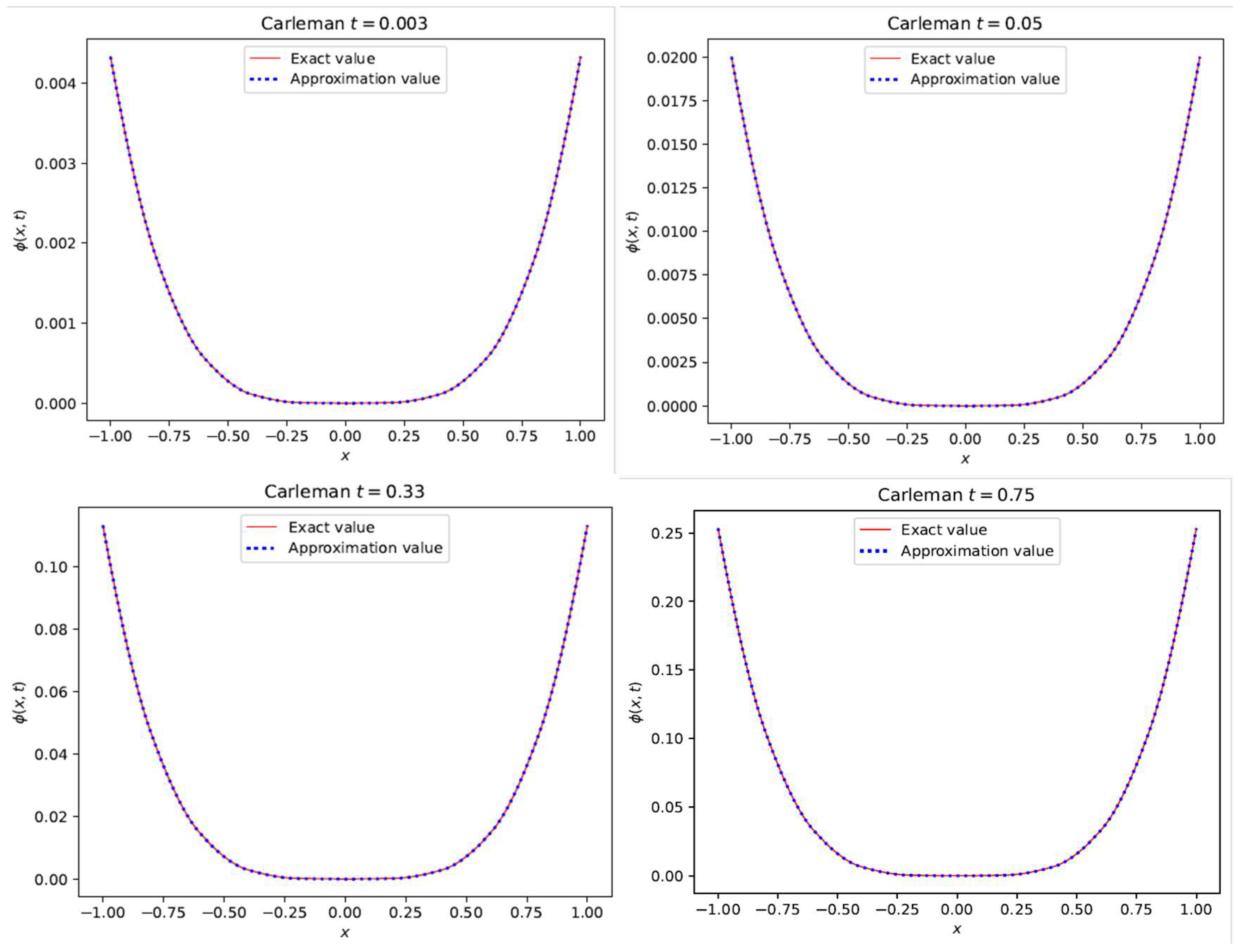
In this case, the kernel is set as a Carleman function, such that  $k\left(\left|x-y\right|\right)={\left|x-y\right|}^{-\upsilon },0<\upsilon <1.$ The exact solution, numerical solution, and absolute error between the approximation of $\Phi \left(x_i,t\right)$ and the exact solution at various time steps (i.e., at $t=0.003, 0.05, 0.33, \mathit{and} 0.75)$ are presented in 

Table 1. The exact, numerical, and absolute error results for Equation (35) with a Carleman kernel at $t=0.003 \mathrm{and} 0.05$

x	$\mathit{T}=0.003$			$\mathit{T}=0.05$
	Exact Sol.	Num. Sol.	Abs. Error	Exact Sol.	Num. Sol.	Abs. Error
−1	0.004333333	0.00433283	5.03737 × 10−7	0.02	0.019997672	2.32774 × 10−6
−0.8	0.001774933	0.001774349	5.83978 × 10−7	0.008192	0.008189301	2.69852 × 10−6
−0.6	0.0005616	0.000560477	1.12265 × 10−6	0.002592	0.002586816	5.18355 × 10−6
−0.4	0.000110933	0.000109273	1.65994 × 10−6	0.000512	0.000504338	7.66196 × 10−6
−0.2	6.93333 × 10−6	4.89595 × 10−6	2.03738 × 10−6	0.000032	2.2597 × 10−5	9.40295 × 10−6
0.0	0	2.1682 × 10−6	2.1682 × 10−6	0	1.00064 × 10−5	1.00064 × 10−5
0.2	6.93333 × 10−6	4.89595 × 10−6	2.03738 × 10−6	0.000032	2.2597 × 10−5	9.40295 × 10−6
0.4	0.000110933	0.000109273	1.65994 × 10−6	0.000512	0.000504338	7.66196 × 10−6
0.6	0.0005616	0.000560477	1.12265 × 10−6	0.002592	0.002586816	5.18355 × 10−6
0.8	0.001774933	0.001774349	5.83978 × 10−7	0.008192	0.008189301	2.69852 × 10−6
1	0.004333333	0.00433283	5.03737 × 10−7	0.02	0.019997672	2.32774 × 10−6

and

Table 2. The exact, numerical, and absolute error results for Equation (35) with a Carleman kernel at $t=0.33 \mathrm{and} 0.75$.

x	$\mathit{T}=0.33$			$\mathit{T}=0.75$
	Exact Sol.	Num. Sol.	Abs. Error	Exact Sol.	Num. Sol.	Abs. Error
−1	0.1133333	0.11331946	1.38735 × 10−5	0.253333333	0.253300963	3.23704 × 10−5
−0.8	0.0464213	0.046405254	1.60789 × 10−5	0.103765333	0.103727829	3.75044 × 10−5
−0.6	0.014688	0.014658118	2.98824 × 10−5	0.032832	0.032764178	6.78217 × 10−5
−0.4	0.0029013	0.002857737	4.35962 × 10−5	0.006485333	0.006387495	9.78387 × 10−5
−0.2	0.0001813	0.000128121	5.32124 × 10−5	0.000405333	0.000286479	0.000118854
0.0	0	−5.66404 × 10−5	5.66404 × 10−5	0	−0.00012634	0.00012634
0.2	0.0001813	0.000128121	5.32124 × 10−5	0.000405333	0.000286479	0.000118854
0.4	0.0029013	0.002857737	4.35962 × 10−5	0.006485333	0.006387495	9.78387 × 10−5
0.6	0.014688	0.014658118	2.98824 × 10−5	0.032832	0.032764178	6.78217 × 10−5
0.8	0.0464213	0.046405254	1.60789 × 10−5	0.103765333	0.103727829	3.75044 × 10−5
1	0.1133333	0.11331946	1.38735 × 10−5	0.253333333	0.253300963	3.23704 × 10−5

 for points $x\in \left[-1, 1\right],$ with the choice of $\upsilon =0.28$. Figure 1 illustrates the convergence of the numerical solution to the exact solution at each time. As expected, the cumulative effects of approximation lead to an increase in error over time.

Application 2. 

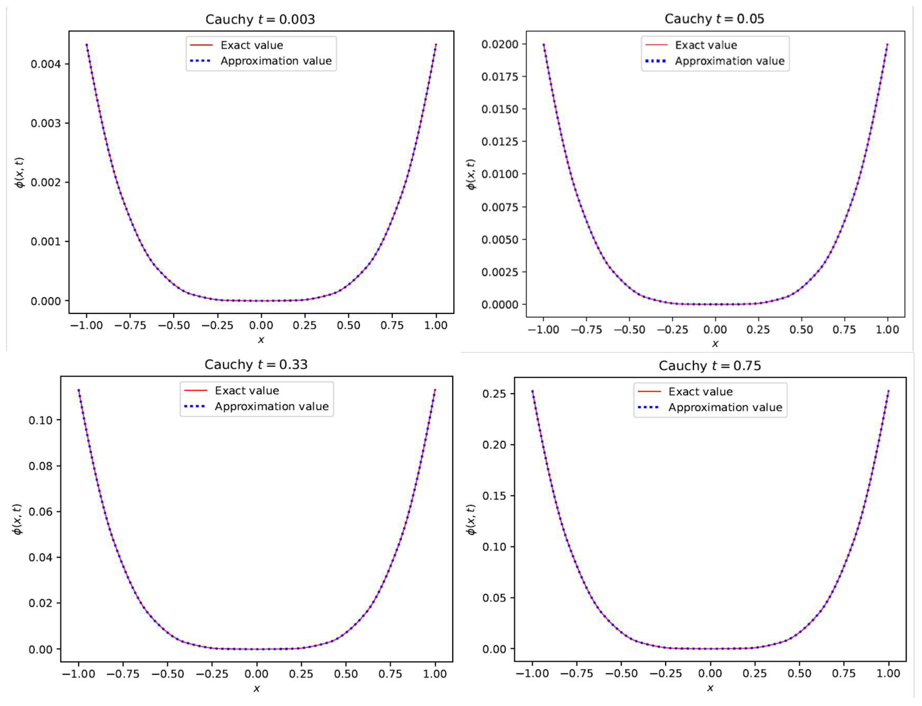
In this case, a Cauchy kernel is used, such that  $k(\left|x-y\right|)={\displaystyle \frac{1}{(x-y)}}$. The exact solution, numerical solution, and absolute error at $t=0.003, 0.05, 0.33, \mathit{and} 0.75$ are presented in

Table 3. The exact, numerical, and absolute error results for Equation (35) with a Cauchy kernel at $t=0.003 \mathrm{and} 0.05$.

x	$\mathit{T}=0.003$			$\mathit{T}=0.05$
	Exact Sol.	Num. Sol.	Abs. Error	Exact Sol.	Num. Sol.	Abs. Error
−1	0.004333333	0.004332411	9.22315 × 10−7	0.02	0.019995743	4.25694 × 10−6
−0.8	0.001774933	0.001774369	5.64143 × 10−7	0.008192	0.008189396	2.60376 × 10−6
−0.6	0.0005616	0.000561247	3.52765 × 10−7	0.002592	0.002590372	1.62816 × 10−6
−0.4	0.000110933	0.000110745	1.88774 × 10−7	0.000512	0.000511129	8.71273 × 10−7
−0.2	6.93333 × 10−6	6.84601 × 10−6	8.73267 × 10−8	0.000032	3.1597 × 10−5	4.03049 × 10−7
0.0	0	−5.31103 × 10−8	5.31103 × 10−8	0	−2.45126 × 10−7	2.45126 × 10−7
0.2	6.93333 × 10−6	6.84601 × 10−6	8.73267 × 10−8	0.000032	3.1597 × 10−5	4.03049 × 10−7
0.4	0.000110933	0.000110745	1.88774 × 10−7	0.000512	0.000511129	8.71273 × 10−7
0.6	0.0005616	0.000561247	3.52765 × 10−7	0.002592	0.002590372	1.62816 × 10−6
0.8	0.001774933	0.001774369	5.64143 × 10−7	0.008192	0.008189396	2.60376 × 10−6
1	0.004333333	0.004332411	9.22315 × 10−7	0.02	0.019995743	4.25694 × 10−6

and

Table 4. The exact, numerical, and absolute error results for Equation (35) with a Cauchy kernel at $t=0.33 \mathrm{and} 0.75$.

x	$\mathit{T}=0.33$			$\mathit{T}=0.75$
	Exact Sol.	Num. Sol.	Abs. Error	Exact Sol.	Num. Sol.	Abs. Error
−1	0.1133333	0.113309185	2.41487 × 10−5	0.25333333	0.253279301	5.40323 × 10−5
−0.8	0.0464213	0.046406572	1.47613 × 10−5	0.10376533	0.103732324	3.30093 × 10−5
−0.6	0.014688	0.01467877	9.23021 × 10−6	0.032832	0.03281136	2.06402 × 10−5
−0.4	0.0029013	0.002896394	4.93915 × 10−6	0.00648533	0.006474289	1.10444 × 10−5
−0.2	0.0001813	0.000179049	2.28465 × 10−6	0.00040533	0.000400225	5.10831 × 10−6
0.0	0	−1.3591 × 10−6	1.3591 × 10−6	0	−3.10619 × 10−6	3.10619 × 10−6
0.2	0.0001813	0.000179049	2.28465 × 10−6	0.00040533	0.000400225	5.10831 × 10−6
0.4	0.0029013	0.002896394	4.93915 × 10−6	0.00648533	0.006474289	1.10444 × 10−5
0.6	0.014688	0.01467877	9.23021 × 10−6	0.032832	0.03281136	2.06402 × 10−5
0.8	0.0464213	0.046406572	1.47613 × 10−5	0.10376533	0.103732324	3.30093 × 10−5
1	0.1133333	0.113309185	2.41487 × 10−5	0.25333333	0.253279301	5.40323 × 10−5

$,$ where $x\in \left[-1, 1\right].$ The convergence of the numerical solution to the exact solution at each time is displayed in Figure 2. The error increases with time due to the cumulative effects of approximation, which is to be expected.

Application 3. 

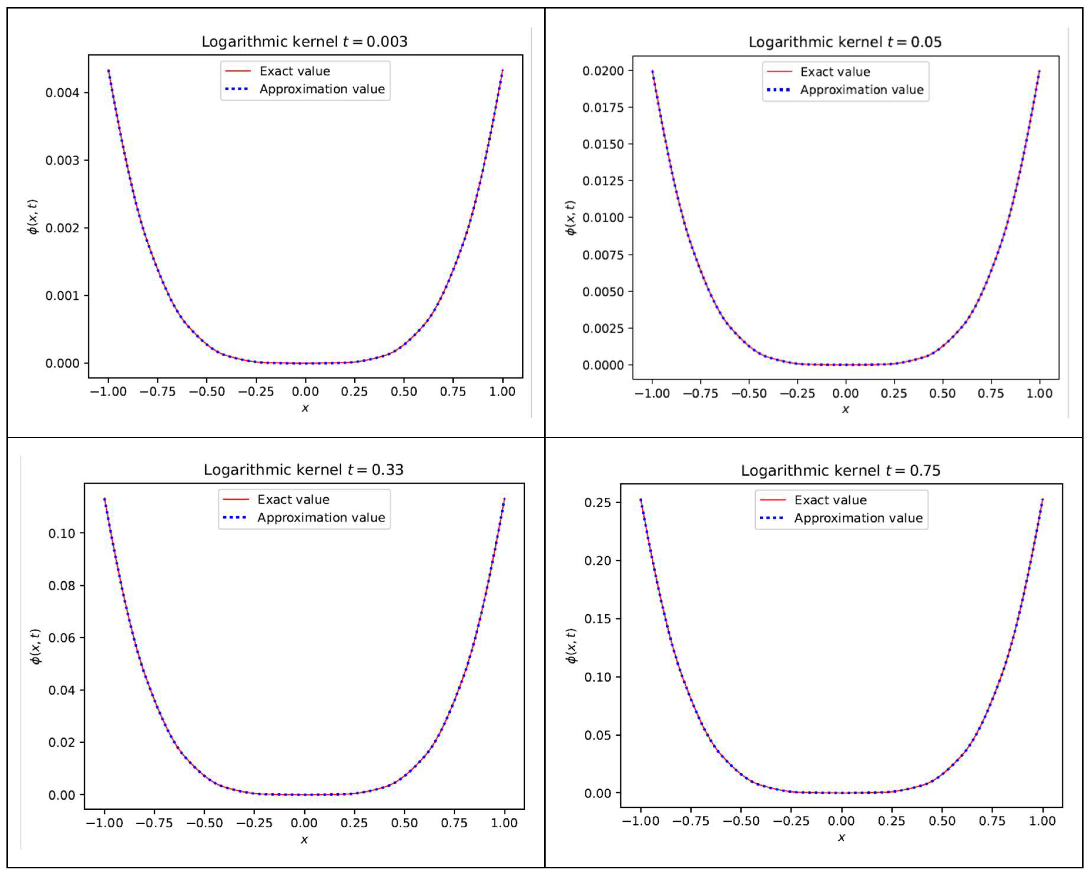
In this case, the kernel takes the logarithmic type such that $k\left(\right|x-y\left|\right)=\mathrm{l}\mathrm{n} | x-y|$.

Table 5. The exact, numerical, and absolute error results for Equation (35) with a logarithmic kernel at $t=0.003 \mathrm{and} 0.05$.

x	$\mathit{T}=0.003$			$\mathit{T}=0.05$
	Exact Sol.	Num. Sol.	Abs. Error	Exact Sol.	Num. Sol.	Abs. Error
−1	0.004333333	0.004330633	2.69999 × 10−6	0.02	0.019987541	1.24588 × 10−5
−0.8	0.001774933	0.001771622	3.31099 × 10−6	0.008192	0.008176721	1.52787 × 10−5
−0.6	0.0005616	0.000559283	2.31729 × 10−6	0.002592	0.002581306	1.06936 × 10−5
−0.4	0.000110933	0.000109609	1.32472 × 10−6	0.000512	0.000505887	6.11347 × 10−6
−0.2	6.93333 × 10−6	6.27967 × 10−6	6.53662 × 10−7	0.000032	2.89832 × 10−5	3.01683 × 10−6
0.0	0	4.19637 × 10−7	4.19637 × 10−7	0	1.93691 × 10−6	1.93691 × 10−6
0.2	6.93333 × 10−6	6.27967 × 10−6	6.53662 × 10−7	0.000032	2.89832 × 10−5	3.01683 × 10−6
0.4	0.000110933	0.000109609	1.32472 × 10−6	0.000512	0.000505887	6.11347 × 10−6
0.6	0.0005616	0.000559283	2.31729 × 10−6	0.002592	0.002581306	1.06936 × 10−5
0.8	0.001774933	0.001771622	3.31099 × 10−6	0.008192	0.008176721	1.52787 × 10−5
1	0.004333333	0.004330633	2.69999 × 10−6	0.02	0.019987541	1.24588 × 10−5

and

Table 6. The exact, numerical, and absolute error results for Equation (35) with a logarithmic kernel at $t=0.33 \mathrm{and} 0.75$.

x	$\mathit{T}=0.33$			$\mathit{T}=0.75$
	Exact Sol.	Num. Sol.	Abs. Error	Exact Sol.	Num. Sol.	Abs. Error
−1	0.1133333	0.113263398	6.99354 × 10−5	0.25333333	0.253178331	0.000155003
−0.8	0.0464213	0.04633543	8.59038 × 10−5	0.10376533	0.103574664	0.000190669
−0.6	0.014688	0.01462779	6.02104 × 10−5	0.032832	0.032698187	0.000133813
−0.4	0.0029013	0.002866847	3.44859 × 10−5	0.00648533	0.006408564	7.67695 × 10−5
−0.2	0.0001813	0.000164255	1.7078 × 10−5	0.00040533	0.000367196	3.8137 × 10−5
0.0	0	1.10049 × 10−5	1.10049 × 10−5	0	2.46552 × 10−5	2.46552 × 10−5
0.2	0.0001813	0.000164255	1.7078 × 10−5	0.00040533	0.000367196	3.81373 × 10−5
0.4	0.0029013	0.002866847	3.44859 × 10−5	0.00648533	0.006408564	7.67695 × 10−5
0.6	0.014688	0.01462779	6.02104 × 10−5	0.032832	0.032698187	0.000133813
0.8	0.0464213	0.04633543	8.59038 × 10−5	0.10376533	0.103574664	0.000190669
1	0.1133333	0.113263398	6.99354 × 10−5	0.25333333	0.253178331	0.000155003

present the exact solution, numerical solution, and their corresponding absolute errors at $x\in \left[-1, 1\right]$ for $t=0.003, 0.05, 0.33, \mathit{and} 0.75$. Figure 3 illustrates the convergence of the numerical solution to the exact solution at each time point. As expected, the cumulative effects of approximation lead to an increase in error over time.

Application 4. 

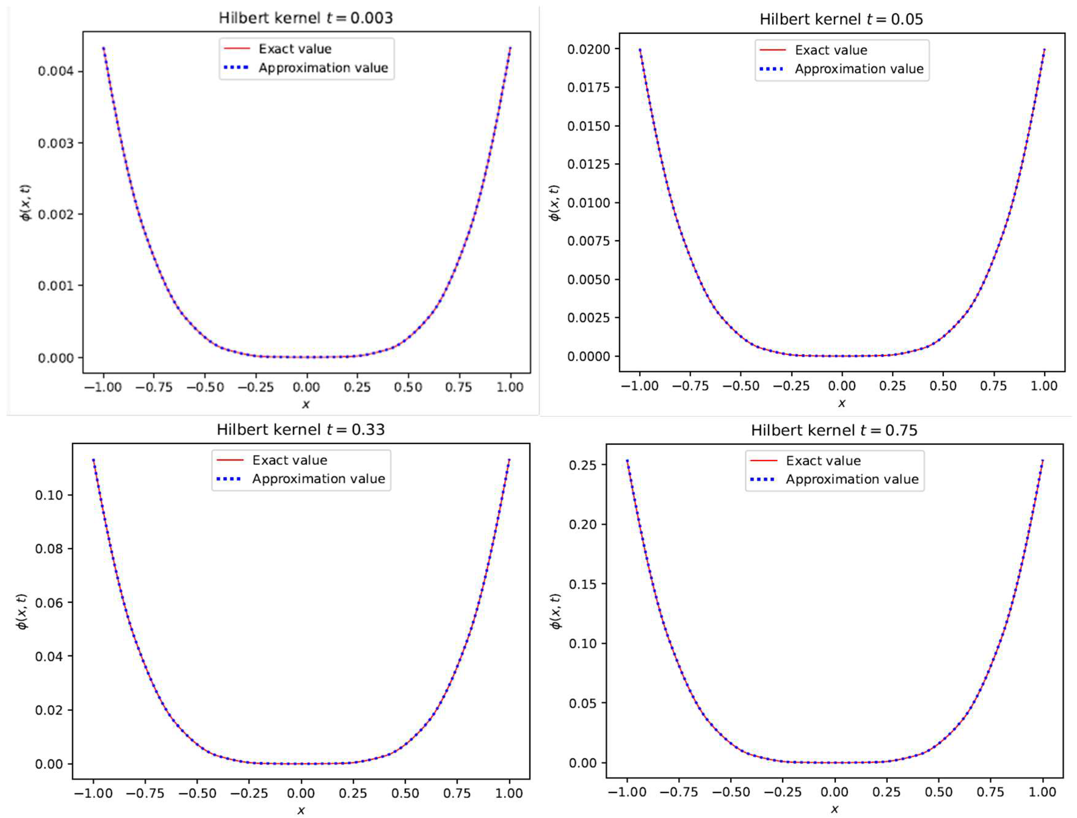
In this case, a Hilbert kernel is used such that $k(\left|x-y\right|)=cot ( {\displaystyle \frac{x-y}{2}}), x\in \left[-1,1\right]$. The exact solution, numerical solution, and absolute error at $t=0.003, 0.05, 0.33, and 0.75$ are presented in 

Table 7. The exact, numerical, and absolute error results for Equation (35) with a Hilbert kernel at $t=0.003 \mathrm{and} 0.05$.

x	$\mathit{T}=0.003$			$\mathit{T}=0.05$
	Exact Sol.	Num. Sol.	Abs. Error	Exact Sol.	Num. Sol.	Abs. Error
−1	0.004333333	0.00433253	8.03563 × 10−7	0.02	0.019996723	3.27679 × 10−6
−0.8	0.001774933	0.001774428	5.05264 × 10−7	0.008192	0.008189744	2.25593 × 10−6
−0.6	0.0005616	0.000561283	3.16827 × 10−7	0.002592	0.002590559	1.44115 × 10−6
−0.4	0.000110933	0.000110763	1.69968 × 10−7	0.000512	0.000511217	7.82779 × 10−7
−0.2	6.93333 × 10−6	6.85438 × 10−6	7.8953 × 10−8	0.000032	3.16333 × 10−5	3.66728 × 10−7
0.0	0	−4.82325 × 10−8	4.82325 × 10−8	0	−2.25 × 10−7	2.25024 × 10−7
0.2	6.93333 × 10−6	6.85438 × 10−6	7.8953 × 10−8	0.000032	3.16333 × 10−5	3.66728 × 10−7
0.4	0.000110933	0.000110763	1.69968 × 10−7	0.000512	0.000511217	7.82779 × 10−7
0.6	0.0005616	0.000561283	3.16827 × 10−7	0.002592	0.002590559	1.44115 × 10−6
0.8	0.001774933	0.001774428	5.05264 × 10−7	0.008192	0.008189744	2.25593 × 10−6
1	0.004333333	0.00433253	8.03563 × 10−7	0.02	0.019996723	3.27679 × 10−6

and

Table 8. The exact, numerical, and absolute error results for Equation (35) with a Hilbert kernel at $t=0.33 \mathrm{and} 0.75$.

x	$\mathit{T}=0.33$			$\mathit{T}=0.75$
	Exact Sol.	Num. Sol.	Abs. Error	Exact Sol.	Num. Sol.	Abs. Error
−1	0.1133333	0.113430772	9.74382 × 10−5	0.25333333	0.254350998	0.001017664
−0.8	0.0464213	0.046428971	7.63729 × 10−6	0.10376533	0.103923162	0.000157828
−0.6	0.014688	0.014685504	2.49603 × 10−6	0.032832	0.032865509	3.35091 × 10−5
−0.4	0.0029013	0.002897351	3.98236 × 10−6	0.00648533	0.006479559	5.7746 × 10−6
−0.2	0.0001813	0.00017863	2.70364 × 10−6	0.00040533	0.000394979	1.03544 × 10−5
0.0	0	−1.92292 × 10−6	1.92292 × 10−6	0	−8.76 × 10−6	8.76338 × 10−6
0.2	0.0001813	0.00017863	2.70364 × 10−6	0.00040533	0.000394979	1.03544 × 10−5
0.4	0.0029013	0.002897351	3.98236 × 10−6	0.00648533	0.006479559	5.7746 × 10−6
0.6	0.014688	0.014685504	2.49603 × 10−6	0.032832	0.032865509	3.35091 × 10−5
0.8	0.0464213	0.046428971	7.63729 × 10−6	0.10376533	0.103923162	0.000157828
1	0.1133333	0.113430772	9.74382 × 10−5	0.25333333	0.254350998	0.001017664

, where $x\in \left[-1, 1\right].$ The convergence of the numerical solution to the exact solution at each time point is displayed in Figure 4. Again, the error increases with time due to the cumulative effects of approximation, which is to be expected.

In this case, we apply the following formula (see Gradshteyn and Ryzhik [21]) to determine the integral in Equation (38):

$$\int u^p \mathrm{c}\mathrm{o}\mathrm{t} u du =\sum _{s=0}^{\infty }{\displaystyle \frac{(-1{)}^s{2}^{2s}{B}_{2s}}{\left(p+2s\right)\left(2s\right)!}} u^{p+2s}, [p\ge 1,|u|<\pi ]$$

(40)

where $B_{2s}$ are Bernoulli numbers.

The exponential generating function may be used to define the sequence of rational numbers known as the Bernoulli numbers $B_s$.

$${\displaystyle \frac{u}{e^u-1}}=\sum _{s=0}^{\infty }{\displaystyle \frac{u^s{B}_s}{s!}} , 0<\left|u\right|<\pi .$$

These numbers have the following general form, as they appear in the series expansions of trigonometric functions:

$$B_{2s}=(-1{)}^{s+1}4s{\int }_0^{\infty }{\displaystyle \frac{u^{2s-1}}{e^{2\pi u}-1}} du, s=1,2,\cdots$$

To further illustrate the accuracy performance of the numerical scheme, the $L^{\infty } error$ (maximum error total position points) and the $L^2 error$(the Euclidean norm) were calculated as follows:

$$L^{\infty }error=\underset{-N\le i\le N,}{\mathrm{m}\mathrm{a}\mathrm{x}} \left|\Phi \left(x_i,t\right)-{\Phi }_N\left(x_i,t\right)\right|,$$

and

$$L^{2}error={\left(\sum _{i=-N}^N{\left|\Phi \left(x_i,t\right)-{\Phi }_N\left(x_i,t\right)\right|}^2 \right)}^{1/2}.$$

Table 9. Comparison of the $L^2$ and $L^{\infty }$ error values for the Carleman and Cauchy kernels over time $t\in \left[0,T\right].$

T	Carleman		Cauchy
	${\mathit{L}}^2$ − Error	${\mathit{L}}^{\mathit{\infty }}$ − Error	${\mathit{L}}^2$ − Error	${\mathit{L}}^{\mathit{\infty }}$ − Error
0	1.01880 × 10−5	1.67079 × 10−6	2.77062 × 10−6	7.09472 × 10−7
0.003	1.32444 × 10−5	2.1682 × 10−6	3.60181 × 10−6	9.22315 × 10−7
0.05	6.11337 × 10−5	1.00064 × 10−5	1.66239 × 10−5	4.25694 × 10−6
0.33	3.47878 × 10−4	5.66404 × 10−5	9.42519 × 10−5	2.41487 × 10−5
0.75	7.80878 × 10−4	1.26340 × 10−4	2.10782 × 10−4	5.40323 × 10−5
1	2.82578 × 10−3	1.32989 × 10−4	2.76620 × 10−4	7.07163 × 10−5

displays the $L^2$ and $L^{\infty }$ errors for the Carleman and Cauchy kernels, while

Table 10. Comparison of the $L^2$ and $L^{\infty }$ error values for the logarithmic and Hilbert kernels over time $t\in [0,T]$.

T	Logarithmic		Hilbert
	${\mathit{L}}^2$ − Error	${\mathit{L}}^{\mathit{\infty }}$ − Error	${\mathit{L}}^2$ − Error	${\mathit{L}}^{\mathit{\infty }}$ − Error
0	1.08405 × 10−5	2.07691 × 10−6	2.47182 × 10−6	6.18196 × 10−7
0.003	1.40927 × 10−5	3.31099 × 10−6	3.21323 × 10−6	8.03563 × 10−7
0.05	6.50319 × 10−5	1.52787 × 10−5	1.41696 × 10−5	3.27679 × 10−6
0.33	3.65763 × 10−4	8.59038 × 10−5	1.61935 × 10−4	9.74382 × 10−5
0.75	8.12089 × 10−4	1.90669 × 10−4	1.857819 × 10−3	1.017664 × 10−3
1	3.12479 × 10−3	1.08833 × 10−3	2.88556 × 10−3	1.57213 × 10−3

displays these errors for the Hilbert and logarithmic kernels.

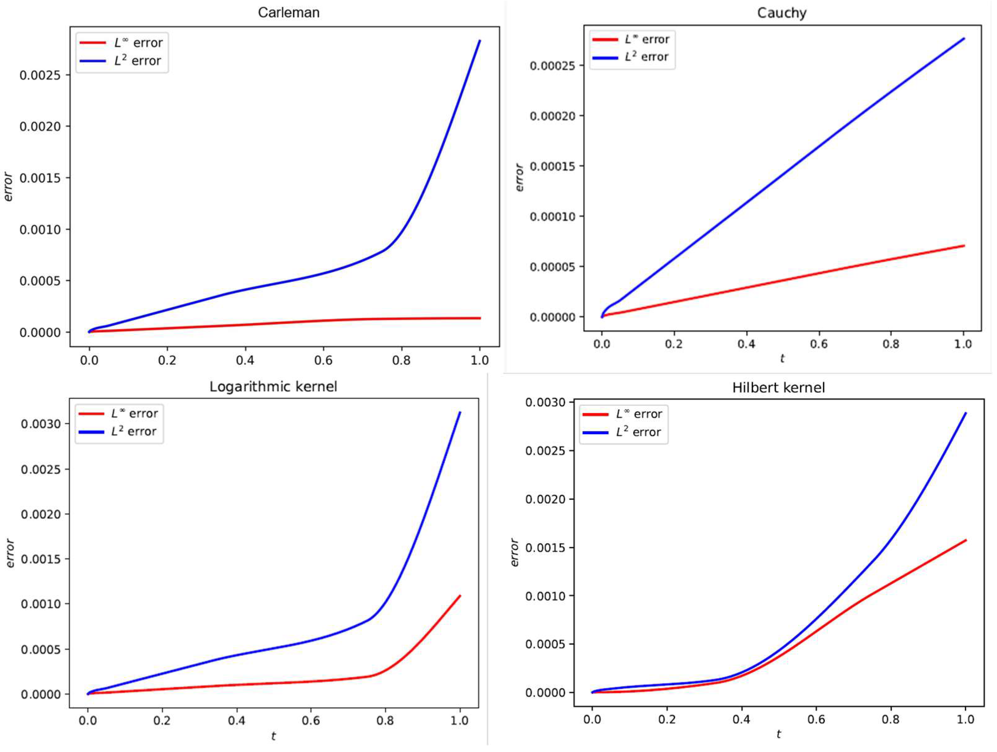
Figure 5 illustrates how the numerical accuracy in terms of the $L^2$ and $L^{\infty }$ errors changes over time, divided into four subfigures to cover all four studied kernels. Both errors exhibit a clear growth pattern over time, reflecting the accumulation of approximation errors. The two curves remain on the same order of magnitude for all cases, demonstrating the stability of the numerical method on normed spaces; however, the $L^2$ error grows more rapidly than the $L^{\infty }$ error.

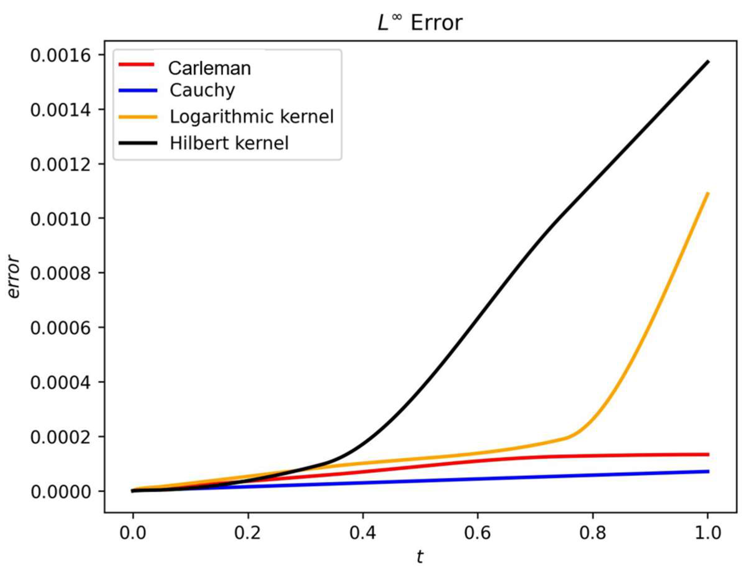
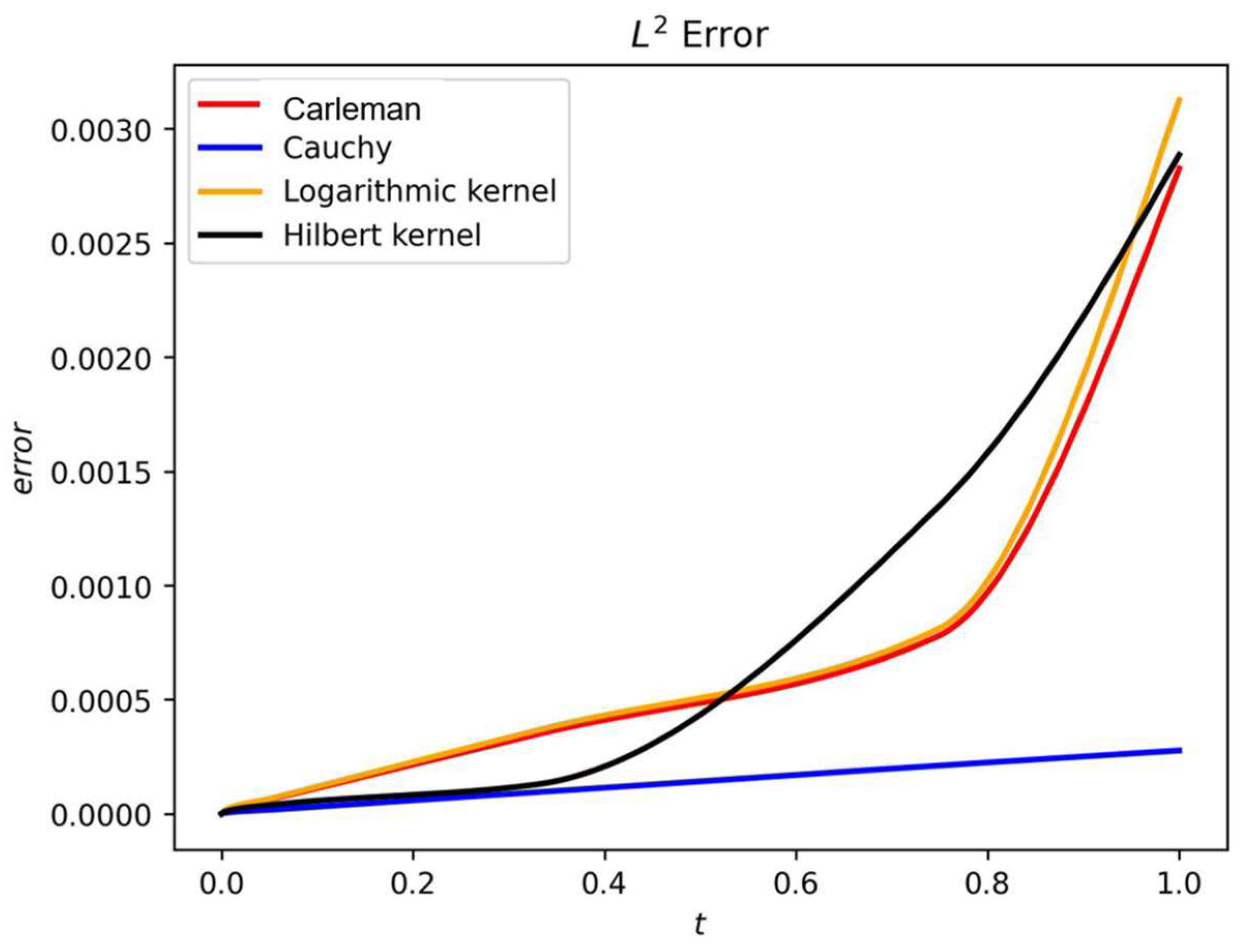
Figure 6 compares the $L^{\infty }$ error levels of solutions with several kernel types (Carleman, Cauchy, Hilbert, and logarithmic) over time, while Figure 7 displays the $L^2$ error levels for these kernels. The results indicate that, although the error values remain small in all scenarios, the type of kernel affects the error behavior; in particular, the Cauchy kernel exhibited the lowest error in both figures, whereas the Hilbert kernel exhibited the highest error.

11. Discussion of Numerical Results

An overview of the results obtained for the considered applications is given below.

• When using the Carleman, Cauchy, and logarithmic kernels, the errors are smallest around the center of the position interval and significantly higher at the limits (i.e., $x=\pm 1$), as detailed in Table 1, Table 2, Table 3, Table 4, Table 5 and Table 6. These kernels have a greater influence close to the boundary, where numerical computation and approximation errors are often more apparent, explaining this predicted behavior. Nevertheless, even at the limits, the errors remain exceedingly modest, indicating the strength of the method.
• When using the Hilbert kernel, the errors are highest around the center of the position interval and significantly lower at the limits ($x=\pm 1$), as detailed in Table 7 and Table 8. However, even at the center, the error values remain small.
• From Figure 1, Figure 2, Figure 3 and Figure 4, it can be seen that the numerical solutions obtained in each of the cases were very close to the exact solutions, demonstrating the effectiveness and significant dependability of the techniques presented in this paper.
• In addition to the values given in Table 9 and Table 10, Figure 5 makes it evident that the $L^{\infty }$, $L^2$, and absolute errors increase with time, becoming more noticeable at $T\approx 1$ throughout the position range.
• Figure 6 and Figure 7 clearly show that both the $L^{\infty }$ and $L^2$ errors reached their highest values when a Hilbert-type kernel was used. In contrast, solutions obtained with the Cauchy kernel achieved the highest level of accuracy.

12. Conclusions

The following conclusions were reached:

• In this article, a novel approach for the extensive analytical and numerical investigation of I-PDEs with singular kernels was presented. A general I-PDE was converted into a mixed integral equation, enabling a comprehensive analysis of convergence and the existence of solutions.
• The Banach fixed-point theorem was used to demonstrate the existence of a unique solution. The reader might also obtain the same result using the Picard technique, which is a successive approximation approach.
• We employed the separation of variables technique to simplify the MIE, following which the TMM was applied to solve the resulting Fredholm integral equation.
• An algebraic system with a coefficient that is a function of time was obtained using the TMM. Subsequently, the existence of a unique solution for the algebraic system in the Banach space $l^{\infty }$ was investigated.
• The results indicated that the numerical technique achieves a high level of accuracy and exhibits stable convergence, illustrating the effectiveness of the numerical methods utilized. Furthermore, it is possible to extend the proposed approach to include more categories of integral equations, integro-differential equations, and more complicated computational applications.

13. Future Work

Future research should investigate the application of generalized methods to address higher-level nonlinearities of partial integro-differential equations, which may culminate in the resolution of various nonlinear elasticity-related applications. Furthermore, the accuracy and efficacy of these algorithms could be improved by adding new methods.