Color Image Multi-Threshold Segmentation Based on Modified Reptile Search Algorithm

Abstract

Multi-threshold image segmentation is a common technique in computer vision and image analysis. However, segmentation quality suffers greatly as the number of thresholds increases, particularly for color image segmentation tasks. To address this challenge, this paper proposes a modified reptile search algorithm (MRSA) based on Otsu and Kapur objective functions. Firstly, an RSA algorithm is developed by combining an adaptive weight factor and elite-guided learning to improve segmentation performance. Secondly, an RGB channel symmetric cooperation mechanism is introduced to exchange information among color channels. Thirdly, a repair mechanism is designed to maintain the structural symmetry of solutions throughout the optimization process. We conduct extensive experiments on the BSD500 benchmark color images under different threshold levels and compare MRSA with an improved bald eagle search algorithm (IBES), enhanced Giza pyramids construction algorithm (GGPC), multi-mechanism artificial lemming algorithm (MALA), and RSA. The experimental results demonstrate that the proposed MRSA algorithm achieves superior segmentation performance in terms of objective function values, region covering, peak signal-to-noise ratio, structural similarity index measure, and feature similarity index, and it exhibits excellent results even at high threshold levels.

1. Introduction

Image processing is a fundamental research area in computer vision and artificial intelligence for extracting meaningful information from visual data [1]. It covers a wide range of tasks, including image enhancement, restoration, classification, object detection, and segmentation [2]. With the rapid growth of data acquisition technologies and the increasing demand for intelligent analysis, image processing techniques have evolved significantly over the past decades [3].

Image segmentation is essential for image processing tasks as it bridges the gap between low-level image representation and high-level semantic comprehension [4]. It divides an image into homogeneous and meaningful regions, and simplifies object recognition and scene analysis [5]. According to existing literature, segmentation techniques can be broadly categorized into threshold-, edge-, and region-based methods [6,7]. Threshold-based segmentation is still highly appealing because of its simplicity and interpretability [8].

Traditional thresholding methods, such as Otsu and Kapur, have been widely used due to their strong theoretical foundations [9]. The Otsu method, based on statistical variance analysis, determines the optimal threshold by maximizing the between-class variance to achieve the best separation between different regions in an image [10]. Kapur entropy adopts information theory and selects thresholds that maximize the total entropy of all segmented regions. The Otsu method is effective for images with clear intensity differences, while Kapur entropy is more suitable for complex images with diverse or multimodal gray-level distributions. However, these approaches are typically limited to grayscale images, and they may lose significant information by ignoring the intrinsic correlations among color channels [11]. It has become an important research direction to expand threshold-based segmentation to color images and incorporate multiple complementary features.

Unlike bi-threshold, multi-threshold divides an image into several regions by determining a set of optimal thresholds [12,13]. The improvement in efficiency comes from the characteristics of the multi-level optimization problem. For an image with $L=256$ gray levels and K thresholds, an exhaustive search requires evaluating $\left({\displaystyle \genfrac{}{}{0pt}{}{256}{K}}\right)$ possible threshold combinations. It makes exhaustive enumeration computationally prohibitive for practical applications. Metaheuristic algorithms have been introduced to search for optimal thresholds using a few fitness evaluations [10]. Particle swarm optimization (PSO), differential evolution (DE), and whale optimization algorithm (WOA) demonstrate promising results in multi-threshold segmentation tasks [14].

More recently, the reptile search algorithm (RSA), inspired by the hunting behavior of crocodiles, has gained attention due to its strong exploration capability [15,16]. We utilize RSA for multi-level thresholding of color images, and the main contributions of this paper are as follows.

• A modified RSA algorithm integrating adaptive weight adjustment and elite-guided learning is proposed to balance exploration and exploitation in multi-threshold image segmentation.
• A symmetric RGB channel collaboration mechanism is developed to exploit complementary inter-channel information for color multi-threshold optimization.
• A solution repair strategy is developed specifically for multi-threshold constraints, which ensures the feasibility and validity of candidate solutions.

The main structure of this paper includes: Section 2 reviews related works on color image multi-threshold segmentation, and Section 3 introduces a novel framework for color image segmentation. Section 4 presents comparative experimental results and analysis, and Section 5 covers the conclusion of our work and its future study.

2. Related Works

Multi-threshold is a fundamental technique in image processing. Recent studies reformulate multi-threshold as an optimization problem and employ metaheuristic algorithms to efficiently approximate optimal solutions.

In color image segmentation, it is crucial to determine the best threshold values. Zhao et al. propose a segmentation method based on an improved mayfly algorithm [17]. A Tent chaotic map initializes the female mayfly population to enhance population diversity, while a Lévy flight mechanism helps the algorithm escape local optima. Artificial rabbits optimization (ARO) is prone to getting stuck in local optima because of its weak local search abilities. Jia et al. improve ARO and validate its effectiveness in multi-threshold color image segmentation using the Otsu method [18]. Furthermore, a center-driven strategy and a Gaussian random walk mechanism enhance the exploration of the algorithm. Song et al. suggest an improved snake optimization (MSO) algorithm using Kapur entropy as the objective function [19]. MSO introduces an adaptive parameter adjustment mechanism, and it combines the guidance of the best individual with random perturbations from other individuals to balance global exploration and local exploitation. MSO segments rice disease images and demonstrates strong potential in agricultural image analysis. Satellite image segmentation has wide applications as it extracts important information from images. Luo et al. propose an improved bald eagle search algorithm (IBES) to find the optimal threshold combination for multi-threshold using Rényi entropy [20]. IBES uses a chaotic tent map and a Lévy flight mechanism to enhance population diversity and expand search space. Amir introduces a hybrid metaheuristic algorithm that utilizes a grey wolf optimizer and cat swarm optimization [21]. A chaotic opposition-based learning strategy improves the algorithm’s efficiency and global search capability.

Image segmentation is an essential step in computer vision. Wu et al. propose an enhanced Giza pyramids construction algorithm (GGPC) [22]. GGPC employs a gradient contour method that utilizes population distribution information to explore the fitness landscape for identifying promising peak regions and providing effective guidance for the subsequent evolutionary process. To better address the multi-threshold image segmentation problem, Rao et al. propose a hybrid adaptive crayfish optimization algorithm (COA) combined with DE [23]. The maximum foraging parameter is optimized to solve the weak convergence performance of the original COA, and an adaptive foraging adjustment strategy is introduced to enhance randomness. In addition, the core update mechanism of DE is incorporated to better balance exploration and exploitation. The search space rapidly expands when the number of thresholds increases, resulting in high computational complexity. Tao et al. bring a multi-mechanism artificial lemming algorithm (MALA) [24]. MALA combines three lightweight mechanisms to guide the population toward optimal solutions and to enhance the management of boundary conditions. Jia et al. present an efficient color image segmentation by implementing a multi-strategy remora optimization algorithm [25]. It incorporates a Beta random restart strategy with prior information to prevent the algorithm from getting trapped in local optima. In addition, a random walk strategy and an elite learning mechanism are integrated to improve convergence speed and solution accuracy. Zhang et al. propose an improved golden jackal optimization algorithm [26]. A high-quality point set is used for population initialization to ensure a more uniform distribution of individuals in the search space and to better handle the complex grayscale characteristics of artistic images. Furthermore, a dual crossover strategy that combines horizontal and vertical information exchange enhances information sharing among individuals and improves fine-grained search capability for meeting the segmentation requirements of textures and color layers in artistic images. A boundary handling mechanism preserves important edge details in artistic images when individuals exceed the search boundaries. Abualigah et al. introduce an improved reptile search algorithm (RSA) [16] in which a Gbest operator enhances its performance. They employ an objective function derived from Otsu and Kapur techniques to determine optimal thresholds for both grayscale and color images. In recent years, robust feature representation and cross-modal information interaction have also been recognized as critical factors for improving visual understanding in complex scenes [27,28].

Table 1. Comparison of representative metaheuristic algorithms for multi-threshold color image segmentation.

Algorithm	Characteristics	Applicable Scenario
[17]	Tent map and Lévy flight	Satellite images
[18]	Gaussian random walk	Color images
[19]	Adaptive parameter adjustment	Rice disease images
[20]	Tent map and Lévy flight	Color images
[21]	Chaotic opposition-based learning	Color images
[22]	Gradient contour guidance	Images with clear object boundaries
[23]	Hybrid of COA and DE	Color images
[24]	Multi-mechanism integration	Low-dimensional threshold
[25]	Beta random restart strategy	Color images
[26]	Uniform initialization and dual crossover	Artistic images
[16]	Gbest operator	Color images

summarizes the characteristics of the representative metaheuristic algorithms reviewed above, along with their applicable scenarios in multi-threshold image segmentation.

Although significant progress has been made, there is still a lack of clear methods to integrate the collaboration mechanism among RGB channels, as well as insufficient utilization of RSA’s global search ability. These limitations motivate the development of an optimization framework for multi-threshold in color images.

3. Multi-Threshold Color Image Segmentation

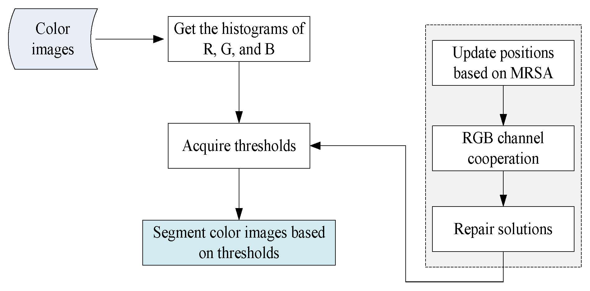
In this section, we suggest a framework for color image segmentation that integrates a modified RSA (MRSA) algorithm, a symmetric RGB channel cooperation mechanism, and a solution repair strategy to improve segmentation quality. Figure 1 illustrates the overall proposed framework.

3.1. Objective Functions

For an image with L gray levels (L = 256), K is the number of thresholds. The threshold vector of a color image I is defined as follows.

$$T^{\left(c\right)}=t_1^{\left(c\right)},t_2^{\left(c\right)},\dots ,t_K^{\left(c\right)},0\le t_1^{\left(c\right)}<t_2^{\left(c\right)}<\cdots <t_K^{\left(c\right)}\le L-1$$

(1)

where c represents a color channel, and $c\in \{R,G,B\}$.

The multi-level thresholding problem can be formulated as a high-dimensional constrained optimization issue.

$$\underset{X}{\max }f\left(X\right)$$

(2)

$$X=\left[T^{\left(R\right)},T^{\left(G\right)},T^{\left(B\right)}\right]$$

(3)

3.1.1. Otsu Method

The thresholds in X divide each channel into K + 1 classes, and it induces a set of regions $C_i^{\left(c\right)}\left(X\right)$ ($i=1,2,\dots ,K+1$). The Otsu method requires that each channel has a maximum between-class variance.

$${\sigma }_B^{\left(c\right)}\left(X\right)={\displaystyle \sum _{i=1}^{K+1}}{\omega }_i^{\left(c\right)}\left(X\right){\left({\mu }_i^{\left(c\right)}\left(X\right)-{\mu }_T^{\left(c\right)}\right)}^2$$

(4)

where ${\omega }_i$ and ${\mu }_i$ denote the probability and mean of the i-th class, respectively, and ${\mu }_T$ is the global mean intensity.

The objective function of multi-level thresholding color image segmentation is defined as follows.

$$f\left(X\right)={\displaystyle \frac{{\sum }_{c\in \{R,G,B\}}{\sigma }_B^{\left(c\right)}\left(X\right)}{3}}$$

(5)

3.1.2. Kapur Entropy

The Kapur entropy of each segmented class is computed based on Shannon entropy, which measures the amount of information contained in a probability distribution.

$$H_i^{\left(c\right)}\left(X\right)=-\sum _{j\in C_i^{\left(c\right)}}{\displaystyle \frac{p_j^{\left(c\right)}}{{\omega }_i^{\left(c\right)}}}\log \left({\displaystyle \frac{p_j^{\left(c\right)}}{{\omega }_i^{\left(c\right)}}}\right)$$

(6)

where $p_j^{\left(c\right)}$ represents the probability of gray level j in channel c, and ${\omega }_i^{\left(c\right)}={\sum }_{j\in C_i^{\left(c\right)}}{p}_j^{\left(c\right)}$ means the total probability of the i-th class.

The optimal threshold set is obtained by maximizing the total entropy over all classes and channels. The average entropy is used to define the objective function to balance the contribution from each color channel.

$$f\left(X\right)={\displaystyle \frac{{\sum }_{c\in \{R,G,B\}}{\sum }_{i=1}^{K+1}{H}_i^{\left(c\right)}\left(X\right)}{3}}$$

(7)

3.2. Modified Reptile Search Algorithm

The reptile search algorithm is a population-based metaheuristic optimization algorithm inspired by the hunting and social behaviors of reptiles. It consists of four behavioral phases used to update positions.

$$X_i^j(t+1)=\left\{\begin{array}{c}Best(1,j)-Eta\ast beta-R\ast randif(t<t_{max}/4)\hfill \\ Best(1,j)\ast X(randi\left(\left[size(X,1)\right]\right),j)\ast ES\ast randif(t<t_{max}/2\&t>=t_{max}/4)\hfill \\ Best(1,j)\ast P\ast randif(t<3\ast t_{max}/4\&t>=t_{max}/2)\hfill \\ Best(1,j)-Eta\ast eps-R\ast randif(t>=3\ast t_{max}/4)\hfill \end{array}\right.$$

(8)

where $X_i$ represents the position of i, j is the dimension, t means the current iteration, $Best$ denotes the global best, and $t_{max}$ is the maximum iteration. R, P, and $Eta$ are acquired with the following equations.

$$R=Best(1,j)-X\left(randi\right(\left[size\right(X,1\left)\right]),j)/\left(\right(Best(1,j))+eps)$$

(9)

$$P=alpha+\left(X\right(i,j)-mean(X(i,:)\left)\right)/\left(Best\right(1,j)\ast (UB-LB)+eps)$$

(10)

$$Eta=Best(1,j)\ast P$$

(11)

where $UB$ and $LB$ represent the upper and lower bounds of the search space, respectively, and $eps$ is a minimum value.

The original update of RSA relies heavily on a single global best solution, which may suffer from decreased population diversity and early convergence in high-dimensional color multi-threshold optimization. We propose an improved update strategy based on adaptive search weight and elite cooperation to achieve a dynamic balance between exploration and exploitation. MRSA retains the population-based optimization framework, initialization procedure, fitness evaluation, and iterative process of RSA, while the original position update mechanism is completely replaced by a new elite collaborative strategy.

• Adaptive weight factor

Inspired by PSO, an adaptive weight factor w is introduced. In early stages, a larger weight increases the search range around the global best solution for enhancing the exploration capability of the population. In later stages, a smaller weight reduces the search range and improves local exploitation accuracy.

$$w=0.9-(0.9-0.5)\ast (t/t_{max})$$

(12)

2.

Update positions

Unlike [16], which depends only on a single global best individual to guide the entire search process, the proposed MRSA constructs a new reference solution by selecting the best threshold components independently from multiple elite individuals for different RGB channels. Therefore, elite information is exploited at the channel level rather than the individual level, which better matches the characteristics of color multi-threshold optimization.

$$[values,idx]=max\left(F_{channel}\left(X\right)\right)$$

(13)

$$best\_sol=[X_{idx\left(1\right)}^{1:K},X_{idx\left(2\right)}^{K+1:2\ast K},X_{idx\left(3\right)}^{2\ast K+1:3\ast K}]$$

(14)

where $F_{channel}$ is a two-dimensional array, with each row representing the Kapur/Otsu values for the R, G, and B channels.

In the exploration stage, each individual updates its position according to the distance information between itself and the current best solution for achieving guided random perturbation. In the exploitation stage, the position is updated using the difference between two elite solutions ($r_1$ and $r_2$) randomly selected from a candidate pool composed of four elite individuals. In addition, a new solution is retained only when its objective function value is better than that of the current solution to improve convergence.

$$X_i^j(t+1)=\left\{\begin{array}{c}best\_so{l}^j-w\ast \left|(X_i^j\left(t\right)-best\_so{l}^j)\right|if(rand<0.5)\hfill \\ best\_so{l}^j+0.5\ast (r_1^j-r_2^j)else\hfill \end{array}\right.$$

(15)

3.3. RGB Channel Symmetric Cooperation Strategy

RGB channels exhibit inherent symmetry because they describe the same scene from different color perspectives. Inspired by this observation, we propose a threshold optimization strategy based on the symmetric cooperation of RGB channels. Since both Kapur and Otsu objective functions are computed directly from histogram distributions, the optimization process primarily depends on the statistical characteristics of channel intensities. Therefore, histogram correlation provides a computationally efficient measure for estimating inter-channel dependencies during threshold evolution. As depicted in Algorithm 1, it achieves cross-channel information interaction and cooperative optimization.

$sol$, $img$, and K represent a multi-threshold solution, a color image, and the number of thresholds, respectively. In lines 1–3, we compute the histogram of each RGB channel. The histogram directly reflects the intensity distribution underlying Otsu and Kapur thresholding, and it is a more appropriate statistical basis for threshold adjustment. $rho\_RG$, $rho\_GB$, and $rho\_BR$ are the correlation coefficients between R, G, and B channels. In lines 10–12, the solution is updated with the channel information. This cooperative mechanism overcomes the limitations of traditional methods that process each channel independently and ignore the intrinsic relationships between channels. The obtained multi-threshold solution maintains structural consistency and color coherence across the three channels. Since the correlation coefficients reflect the global similarity between channels, the proposed strategy guides the thresholds toward a more reasonable joint distribution for improving segmentation accuracy.

Algorithm 1: Channel cooperation

1  R_hist = imhist(img(:,:,1));  2  G_hist = imhist(img(:,:,2));  3  B_hist = imhist(img(:,:,3));  4  rho_RG = corr(R_hist, G_hist);  5  rho_GB = corr(G_hist, B_hist);  6  rho_BR = corr(B_hist, R_hist);  7  R_old = sol(1:K);  8  G_old = sol(K+1:2*K);  9  B_old = sol(2*K+1:3*K); 10  R = R_old + rho_RG*(G_old - R_old); 11  G = G_old + rho_GB*(B_old - G_old); 12  B = B_old + rho_BR*(R_old - B_old); 13  sol = [R G B];

3.4. Solution Repair Strategy

Metaheuristic algorithms exhibit strong randomness during the search process when segmenting multi-threshold color images. The generated threshold solutions may contain out-of-bound values, or even overlapping thresholds. These invalid solutions not only destroy the physical meaning of threshold segmentation but also reduce the stability of fitness evaluation. To address this issue, a solution repair strategy is designed to transform candidate threshold solutions into feasible and valid ones.

As demonstrated in Algorithm 2, the threshold vector is first sorted in ascending order to satisfy the monotonic increasing constraint required in multi-threshold segmentation. Then, a boundary constraint mechanism is applied to limit the thresholds within the valid grayscale range for preventing the algorithm from exploring invalid search regions. Any threshold value falls outside the valid intensity range [0, L− 1]. Finally, a threshold conflict repair mechanism is introduced. When adjacent thresholds overlap, the subsequent thresholds are adaptively increased to ensure sufficient separation between different thresholds.

Algorithm 2: Repair solution

4. Experimental Results and Analysis

To evaluate the effectiveness of the proposed algorithm, we conduct experiments on the BSD500 benchmark color images widely used in image segmentation studies [29]. We randomly choose 20 images from the images of the BSD500 dataset (9 from training, 6 from validation, 5 from test) using a stratified random sampling to ensure a diverse and representative subset that covers various scene types, color distributions, and texture complexities. Among the recently published segmentation methods reviewed in Section 2, IBES [20], GGPC [22], MALA [24], and RSA [16] are considered for experimental comparison. All parameter values for the comparison algorithms listed in

Table 2. The main parameters.

Algorithm	Main Parameters
IBES	a = 10; R_spiral = 1.5; C1 = 1; C2 = 1; alpha_param = 1.5;
GGPC	g = 9.8; theta = pi/6; uk_min = 0.2; uk_max = 0.8; K = 4; omega = 0.5;
MALA	epsilon1 = 0.1; epsilon2 = 0.05;
RSA	beta = 0.1; alpha = 0.1;
MRSA	w = 0.9; beta = 0.1; alpha = 0.1;

are set according to their original publications to ensure a fair and unbiased comparison.

All algorithms have the same population size 20 and a maximum evaluation of 2000. Each algorithm is independently executed 20 times to reduce the influence of randomness. The threshold levels K = 3, 5, and 6 are selected as they represent low-, medium-, and high-complexity scenarios commonly used in multi-threshold segmentation. We also assess their segmentation performance by comparing region covering (RC), peak signal-to-noise ratio (PSNR), structural similarity index measure (SSIM), and feature similarity index (FSIM).

4.1. Comparative Results Based on Kapur Entropy

All experiments are conducted on a PC equipped with an Intel Core i7-6700 CPU @ 3.40 GHz, 12 GB RAM, running Windows 10, and implemented in MATLAB R2020b.

4.1.1. Analysis of the Objective Function Based on Kapur

Table 3. The objective function values using Kapur.

Level	Image	IBES	GGPC	MALA	RSA	MRSA
		Minimum/Mean/STD	Minimum/Mean/STD	Minimum/Mean/STD	Minimum/Mean/STD	Minimum/Mean/STD
3	12003	13.11/13.89/0.63	14.08/15.14/0.29	15.66/15.66/0.0002	14.26/15.53/0.33	15.48/15.62/0.04
	12074	12.13/12.73/0.76	14.70/15.02/0.19	15.38/15.38/0.001	15.13/15.32/0.11	15.24/15.36/0.03
	37073	12.16/13.08/0.64	13.63/14.32/0.30	15.01/15.03/0.01	14.67/14.88/0.1	14.67/14.91/0.09
	58060	13.59/13.96/0.35	14.09/14.67/0.19	15.09/15.10/0.002	14.99/15.05/0.04	14.82/15.01/0.06
	102061	12.13/12.28/0.38	14.48/14.83/0.15	15.26/15.26/0.0006	15.25/15.26/0.002	14.93/15.18/0.08
	210088	12.44/12.49/0.23	14.01/14.94/0.26	15.44/15.46/0.01	14.40/15.35/0.31	15.10/15.39/0.08
	236017	11.91/11.91/0.0002	13.96/14.50/0.21	14.98/14.98/0.004	14.70/14.94/0.10	14.62/14.94/0.10
	253016	12.03/12.03/0.0001	13.73/14.35/0.27	14.92/14.92/0.00008	13.93/14.68/0.43	14.60/14.87/0.06
	257098	12.63/13.28/0.47	14.66/15.38/0.23	15.84/15.84/0.001	14.77/15.73/0.32	15.52/15.76/0.08
	260058	11.62/11.62/0.002	13.21/14.01/0.37	14.61/14.63/0.01	11.54/14.26/0.75	14.34/14.54/0.06
	277095	13.10/13.83/0.22	14.44/14.82/0.16	15.29/15.31/0.01	15.00/15.25/0.09	14.91/15.23/0.12
	296028	11.97/12.01/0.20	14.21/14.50/0.11	14.87/14.87/0.002	13.84/14.66/0.42	14.60/14.83/0.08
	296058	12.44/13.29/0.47	14.27/15.12/0.25	15.65/15.67/0.01	14.56/15.52/0.34	15.38/15.63/0.07
	299091	11.88/11.93/0.21	13.44/14.03/0.29	14.75/14.77/0.01	12.85/14.36/0.56	14.16/14.71/0.12
	309004	12.39/13.22/0.39	14.24/14.80/0.23	15.36/15.42/0.02	15.41/15.43/0.01	14.98/15.37/0.11
	311068	11.37/11.58/0.38	13.04/13.61/0.26	14.35/14.35/0.0002	13.26/14.19/0.29	13.84/14.25/0.10
	374067	12.10/12.21/0.33	14.12/14.65/0.22	15.24/15.28/0.01	15.00/15.24/0.08	14.91/15.18/0.10
	384022	13.78/14.48/0.44	15.10/15.26/0.11	15.65/15.67/0.01	15.37/15.59/0.09	15.39/15.61/0.07
	385028	12.39/12.59/0.42	14.70/15.08/0.16	15.54/15.57/0.01	15.54/15.55/0.01	15.17/15.44/0.07
	393035	10.53/10.82/0.43	12.66/13.08/0.16	13.45/13.45/0.0006	13.32/13.44/0.03	13.26/13.39/0.03
5	12003	18.53/19.55/0.61	19.18/20.03/0.36	16.62/20.80/1.01	16.17/18.92/2.57	20.75/20.93/0.11
	12074	18.38/18.73/0.37	19.14/20.11/0.40	20.77/21.01/0.13	15.92/18.66/3.58	20.53/20.92/0.16
	37073	18.21/18.86/0.34	18.39/19.11/0.33	15.76/20.36/1.10	15.96/18.16/2.59	19.96/20.33/0.2
	58060	18.75/19.47/0.37	18.49/19.44/0.44	20.40/20.56/0.09	14.86/17.79/4.79	19.90/20.47/0.17
	102061	18.17/18.25/0.22	19.53/19.90/0.28	19.93/20.80/0.22	16.00/18.85/3.03	20.28/20.69/0.13
	210088	18.24/18.25/0.004	17.25/19.55/0.64	16.68/20.53/0.95	15.03/17.59/3.26	19.60/20.72/0.29
	236017	17.85/17.90/0.19	17.37/18.83/0.52	19.64/20.35/0.19	15.79/17.06/3.34	18.96/20.15/0.32
	253016	17.57/17.57/0.0003	17.90/18.51/0.37	15.06/19.27/1.38	16.29/18.38/1.60	19.37/19.81/0.19
	257098	18.70/19.30/0.36	19.33/20.11/0.33	20.92/21.27/0.13	16.40/19.57/1.82	21.11/21.20/0.07
	260058	17.43/17.44/0.004	17.31/18.30/0.42	17.03/19.58/0.70	14.57/17.64/2.23	18.86/19.55/0.26
	277095	18.47/19.54/0.37	18.92/19.57/0.29	20.42/20.82/0.14	15.64/18.48/2.52	19.97/20.62/0.25
	296028	17.67/17.74/0.20	18.07/19.03/0.43	19.52/20.13/0.24	15.31/17.53/2.90	19.83/20.15/0.12
	296058	18.62/19.10/0.39	19.69/20.11/0.24	14.29/20.81/1.56	16.05/18.67/2.96	20.52/21.03/0.18
	299091	17.42/17.64/0.37	17.24/18.39/0.58	19.29/19.85/0.22	16.23/18.04/1.96	18.98/19.82/0.21
	309004	18.26/18.86/0.47	18.44/19.57/0.48	15.36/20.37/1.36	15.30/19.09/2.75	19.94/20.72/0.26
	311068	17.00/17.16/0.28	17.16/17.76/0.34	17.87/19.13/0.43	15.11/17.20/2.16	18.35/19.20/0.24
	374067	18.07/18.10/0.01	18.57/19.33/0.47	17.02/20.44/0.83	16.92/18.80/2.09	20.22/20.48/0.18
	384022	18.95/20.14/0.56	19.81/20.32/0.29	20.89/21.23/0.16	16.63/18.96/2.67	20.89/21.20/0.13
	385028	18.33/18.45/0.27	18.85/19.65/0.37	20.63/20.86/0.10	17.76/19.63/0.89	20.14/20.76/0.24
	393035	16.36/16.68/0.42	17.43/18.18/0.30	16.54/18.91/0.58	16.79/17.18/2.04	18.63/18.84/0.15
6	12003	21.21/22.29/0.49	21.05/22.03/0.51	14.22/17.77/5.25	18.31/22.21/1.57	22.99/23.30/0.19
	12074	21.15/21.30/0.28	21.72/22.31/0.31	13.36/16.29/6.60	17.66/21.16/3.30	22.96/23.49/0.20
	37073	21.03/21.64/0.39	20.54/21.15/0.39	13.21/15.42/4.85	16.44/20.89/2.12	21.99/22.81/0.26
	58060	20.73/22.01/0.48	20.67/21.70/0.39	14.38/17.26/5.85	17.36/21.02/3.73	22.45/22.83/0.12
	102061	20.91/20.95/0.19	20.65/21.73/0.47	16.06/18.11/4.02	18.83/20.83/2.99	22.80/23.15/0.17
	210088	20.89/20.89/0.0008	20.78/21.73/0.45	14.93/17.26/5.85	18.46/20.82/2.98	22.33/23.05/0.25
	236017	20.50/20.54/0.15	19.61/20.82/0.46	13.65/16.38/5.36	19.59/21.39/0.89	20.68/22.54/0.49
	253016	20.06/20.06/0.0003	18.92/20.35/0.59	12.29/14.34/4.44	15.66/17.86/3.62	21.62/22.09/0.23
	257098	21.43/21.80/0.35	21.76/22.29/0.34	16.06/18.17/5.48	17.60/20.46/3.31	23.18/23.51/0.21
	260058	19.97/19.98/0.01	18.43/19.70/0.68	12.85/15.60/5.81	16.37/18.90/3.16	21.35/21.70/0.23
	277095	21.78/22.26/0.32	20.44/21.72/0.49	15.57/17.89/4.02	18.56/20.12/2.88	22.25/23.04/0.26
	296028	20.37/20.37/0.0004	20.02/21.13/0.44	14.53/16.57/4.91	17.50/19.87/3.41	21.67/22.37/0.24
	296058	21.37/21.98/0.49	21.76/22.34/0.28	16.42/18.44/3.92	18.84/20.97/2.83	22.56/23.51/0.34
	299091	20.06/20.18/0.23	18.49/20.17/0.67	15.42/17.10/3.78	17.93/19.73/2.84	21.27/22.11/0.22
	309004	20.91/21.33/0.36	20.89/21.69/0.50	15.37/17.73/4.39	18.52/19.80/3.38	21.41/23.09/0.44
	311068	19.49/19.62/0.15	19.57/20.02/0.25	11.01/13.07/6.34	15.52/18.86/3.30	20.77/21.51/0.27
	374067	20.75/20.84/0.19	20.64/21.64/0.43	16.60/18.44/3.85	17.80/19.73/4.18	22.03/22.92/0.29
	384022	22.22/23.05/0.54	21.75/22.55/0.35	16.72/18.52/4.57	19.74/21.13/3.90	23.27/23.69/0.15
	385028	20.97/21.18/0.33	21.01/21.84/0.44	15.66/17.95/5.62	19.22/21.28/2.20	22.48/23.10/0.21
	393035	19.26/19.47/0.45	19.52/20.37/0.38	14.03/16.88/4.41	18.66/20.27/1.96	21.25/21.50/0.17

reports the objective function results using Kapur, including the minimum, average, and standard deviation (STD). The proposed MRSA algorithm achieves the best Kapur values on most test images under different threshold levels. IBES exhibits the weakest performance. As the number of thresholds increases from 3 to 5 and 6, the objective function values of all algorithms show an increasing trend. A larger number of thresholds provides richer partitioning capability and improves image information representation. Compared to the other algorithms, MRSA achieves superior optimization performance in high-dimensional threshold search spaces.

When the number of thresholds is 3, MALA performs best. MRSA ranks among the top two in 18 out of 20 cases, and it is superior to IBES and GGPC. For the images “257098” and “296058”, MRSA achieves results of 15.76 and 15.63, respectively, outperforming RSA. When the threshold number increases to 5, the performance improvement of MRSA becomes more significant. On the images “12003”, “12074”, and “296058”, MRSA achieves values of 20.93, 20.92, and 21.03, respectively, which are clearly better than those of the other algorithms. It is worth mentioning that RSA experiences evident performance degradation on several images, whereas MRSA still manages to obtain high objective function values. In the higher-dimensional threshold segmentation task, the advantages of MRSA become even more obvious, and it outperforms other comparison algorithms. MRSA achieves the best results on all test images, while RSA exhibits large performance fluctuations under high-threshold conditions.

MALA exhibits strong local search capability in low-dimensional search spaces and can quickly reach high-quality solutions. MRSA appears to perform better on most images and it shows great optimization accuracy while preserving strong global exploration ability. Moreover, MRSA demonstrates great adaptability across different types of images.

To further verify the statistical significance of MRSA in multi-threshold color image segmentation, the Wilcoxon rank-sum and Friedman tests are utilized to statistically analyze the experimental results of the algorithms, as shown in

Table 4. Wilcoxon rank-sum test of objective function values based on Kapur.

Level	Image	IBES	GGPC	MALA	RSA	MRSA
3	12003	5.47 $\times {10}^{-8}$	5.56 $\times {10}^{-8}$	-	2.20 $\times {10}^{-3}$	5.56 $\times {10}^{-8}$
	12074	6.39 $\times {10}^{-8}$	6.41 $\times {10}^{-8}$	-	6.62 $\times {10}^{-2}$	1.82 $\times {10}^{-7}$
	37073	6.03 $\times {10}^{-8}$	6.03 $\times {10}^{-8}$	-	6.03 $\times {10}^{-8}$	6.03 $\times {10}^{-8}$
	58060	6.45 $\times {10}^{-8}$	6.49 $\times {10}^{-8}$	-	7.64 $\times {10}^{-7}$	6.49 $\times {10}^{-8}$
	102061	4.65 $\times {10}^{-8}$	4.95 $\times {10}^{-8}$	-	2.70 $\times {10}^{-5}$	4.95 $\times {10}^{-8}$
	210088	6.18 $\times {10}^{-8}$	6.51 $\times {10}^{-8}$	-	6.03 $\times {10}^{-4}$	6.51 $\times {10}^{-8}$
	236017	6.54 $\times {10}^{-8}$	6.71 $\times {10}^{-8}$	-	1.33 $\times {10}^{-2}$	6.71 $\times {10}^{-8}$
	253016	4.11 $\times {10}^{-8}$	4.48 $\times {10}^{-8}$	-	8.74 $\times {10}^{-6}$	4.48 $\times {10}^{-8}$
	257098	6.18 $\times {10}^{-8}$	6.20 $\times {10}^{-8}$	-	2.22 $\times {10}^{-3}$	8.38 $\times {10}^{-8}$
	260058	5.86 $\times {10}^{-8}$	6.26 $\times {10}^{-8}$	-	2.29 $\times {10}^{-6}$	6.26 $\times {10}^{-8}$
	277095	5.94 $\times {10}^{-8}$	5.99 $\times {10}^{-8}$	-	2.04 $\times {10}^{-5}$	5.99 $\times {10}^{-8}$
	296028	6.18 $\times {10}^{-8}$	6.50 $\times {10}^{-8}$	-	1.60 $\times {10}^{-6}$	6.50 $\times {10}^{-8}$
	296058	5.83 $\times {10}^{-8}$	6.01 $\times {10}^{-8}$	-	6.01 $\times {10}^{-3}$	6.01 $\times {10}^{-8}$
	299091	5.35 $\times {10}^{-8}$	5.44 $\times {10}^{-8}$	-	2.95 $\times {10}^{-6}$	5.44 $\times {10}^{-8}$
	309004	5.90 $\times {10}^{-8}$	5.99 $\times {10}^{-8}$	5.63 $\times {10}^{-1}$	-	3.05 $\times {10}^{-7}$
	311068	5.61 $\times {10}^{-8}$	5.73 $\times {10}^{-8}$	-	4.96 $\times {10}^{-6}$	5.73 $\times {10}^{-8}$
	374067	3.74 $\times {10}^{-8}$	3.99 $\times {10}^{-8}$	-	3.50 $\times {10}^{-3}$	5.44 $\times {10}^{-8}$
	384022	5.44 $\times {10}^{-8}$	5.73 $\times {10}^{-8}$	-	1.64 $\times {10}^{-2}$	1.63 $\times {10}^{-7}$
	385028	2.35 $\times {10}^{-8}$	2.44 $\times {10}^{-8}$	-	1.28 $\times {10}^{-5}$	2.44 $\times {10}^{-8}$
	393035	6.21 $\times {10}^{-8}$	6.40 $\times {10}^{-8}$	-	1.05 $\times {10}^{-2}$	6.40 $\times {10}^{-8}$
5	12003	6.80 $\times {10}^{-8}$	6.80 $\times {10}^{-8}$	8.59 $\times {10}^{-2}$	3.71 $\times {10}^{-5}$	-
	12074	6.80 $\times {10}^{-8}$	6.80 $\times {10}^{-8}$	-	1.10 $\times {10}^{-5}$	1.78 $\times {10}^{-3}$
	37073	1.20 $\times {10}^{-6}$	1.20 $\times {10}^{-6}$	-	9.13 $\times {10}^{-7}$	9.05 $\times {10}^{-3}$
	58060	6.80 $\times {10}^{-8}$	6.80 $\times {10}^{-8}$	-	9.75 $\times {10}^{-6}$	1.81 $\times {10}^{-5}$
	102061	6.79 $\times {10}^{-8}$	1.92 $\times {10}^{-7}$	-	2.06 $\times {10}^{-6}$	7.58 $\times {10}^{-6}$
	210088	6.78 $\times {10}^{-8}$	6.01 $\times {10}^{-7}$	8.29 $\times {10}^{-5}$	3.50 $\times {10}^{-6}$	-
	236017	6.80 $\times {10}^{-8}$	6.80 $\times {10}^{-8}$	-	6.80 $\times {10}^{-8}$	9.13 $\times {10}^{-7}$
	253016	6.79 $\times {10}^{-8}$	6.80 $\times {10}^{-8}$	5.79 $\times {10}^{-1}$	2.30 $\times {10}^{-5}$	-
	257098	6.79 $\times {10}^{-8}$	6.80 $\times {10}^{-8}$	-	2.06 $\times {10}^{-6}$	4.70 $\times {10}^{-3}$
	260058	1.12 $\times {10}^{-6}$	2.69 $\times {10}^{-6}$	-	8.29 $\times {10}^{-5}$	3.85 $\times {10}^{-2}$
	277095	6.80 $\times {10}^{-8}$	6.80 $\times {10}^{-8}$	-	6.92 $\times {10}^{-7}$	1.05 $\times {10}^{-6}$
	296028	6.76 $\times {10}^{-8}$	6.80 $\times {10}^{-8}$	2.07 $\times {10}^{-2}$	1.20 $\times {10}^{-6}$	-
	296058	6.79 $\times {10}^{-8}$	6.80 $\times {10}^{-8}$	7.41 $\times {10}^{-5}$	6.22 $\times {10}^{-4}$	-
	299091	6.80 $\times {10}^{-8}$	6.80 $\times {10}^{-8}$	-	1.81 $\times {10}^{-5}$	3.71 $\times {10}^{-5}$
	309004	7.90 $\times {10}^{-8}$	6.92 $\times {10}^{-7}$	8.36 $\times {10}^{-4}$	6.79 $\times {10}^{-2}$	-
	311068	6.80 $\times {10}^{-8}$	9.17 $\times {10}^{-8}$	1.78 $\times {10}^{-3}$	2.30 $\times {10}^{-5}$	-
	374067	6.78 $\times {10}^{-8}$	6.80 $\times {10}^{-8}$	9.09 $\times {10}^{-2}$	9.75 $\times {10}^{-6}$	-
	384022	6.01 $\times {10}^{-7}$	6.80 $\times {10}^{-8}$	-	1.80 $\times {10}^{-6}$	3.34 $\times {10}^{-3}$
	385028	6.76 $\times {10}^{-8}$	6.80 $\times {10}^{-8}$	-	6.01 $\times {10}^{-7}$	7.58 $\times {10}^{-6}$
	393035	2.22 $\times {10}^{-7}$	1.38 $\times {10}^{-6}$	-	1.29 $\times {10}^{-4}$	4.25 $\times {10}^{-1}$
6	12003	6.80 $\times {10}^{-8}$	6.80 $\times {10}^{-8}$	5.87 $\times {10}^{-6}$	2.80 $\times {10}^{-3}$	-
	12074	6.80 $\times {10}^{-8}$	6.80 $\times {10}^{-8}$	3.38 $\times {10}^{-4}$	3.38 $\times {10}^{-4}$	-
	37073	1.43 $\times {10}^{-7}$	7.90 $\times {10}^{-8}$	9.13 $\times {10}^{-7}$	3.50 $\times {10}^{-6}$	-
	58060	2.22 $\times {10}^{-7}$	6.80 $\times {10}^{-8}$	6.92 $\times {10}^{-7}$	1.02 $\times {10}^{-1}$	-
	102061	6.80 $\times {10}^{-8}$	6.80 $\times {10}^{-8}$	1.80 $\times {10}^{-6}$	7.41 $\times {10}^{-5}$	-
	210088	6.80 $\times {10}^{-8}$	1.23 $\times {10}^{-7}$	2.60 $\times {10}^{-5}$	1.44 $\times {10}^{-4}$	-
	236017	9.17 $\times {10}^{-8}$	2.36 $\times {10}^{-6}$	1.78 $\times {10}^{-3}$	6.79 $\times {10}^{-2}$	-
	253016	6.80 $\times {10}^{-8}$	6.80 $\times {10}^{-8}$	3.94 $\times {10}^{-7}$	6.67 $\times {10}^{-6}$	-
	257098	6.80 $\times {10}^{-8}$	6.80 $\times {10}^{-8}$	1.20 $\times {10}^{-6}$	6.87 $\times {10}^{-4}$	-
	260058	6.80 $\times {10}^{-8}$	6.80 $\times {10}^{-8}$	1.10 $\times {10}^{-5}$	5.09 $\times {10}^{-4}$	-
	277095	2.92 $\times {10}^{-5}$	1.23 $\times {10}^{-7}$	7.41 $\times {10}^{-5}$	1.60 $\times {10}^{-5}$	-
	296028	6.80 $\times {10}^{-8}$	9.17 $\times {10}^{-8}$	1.05 $\times {10}^{-6}$	1.61 $\times {10}^{-4}$	-
	296058	2.96 $\times {10}^{-7}$	1.66 $\times {10}^{-7}$	3.05 $\times {10}^{-4}$	8.35 $\times {10}^{-3}$	-
	299091	6.80 $\times {10}^{-8}$	1.06 $\times {10}^{-7}$	5.25 $\times {10}^{-5}$	1.95 $\times {10}^{-3}$	-
	309004	3.94 $\times {10}^{-7}$	1.58 $\times {10}^{-6}$	5.87 $\times {10}^{-6}$	1.04 $\times {10}^{-4}$	-
	311068	6.80 $\times {10}^{-8}$	6.80 $\times {10}^{-8}$	2.22 $\times {10}^{-7}$	2.30 $\times {10}^{-5}$	-
	374067	6.80 $\times {10}^{-8}$	1.92 $\times {10}^{-7}$	6.67 $\times {10}^{-6}$	1.44 $\times {10}^{-4}$	-
	384022	1.23 $\times {10}^{-3}$	6.80 $\times {10}^{-8}$	3.42 $\times {10}^{-7}$	8.29 $\times {10}^{-5}$	-
	385028	6.80 $\times {10}^{-8}$	7.90 $\times {10}^{-8}$	5.90 $\times {10}^{-5}$	2.00 $\times {10}^{-4}$	-
	393035	6.80 $\times {10}^{-8}$	6.80 $\times {10}^{-8}$	9.13 $\times {10}^{-7}$	2.22 $\times {10}^{-4}$	-

. In the results, “-” indicates that the corresponding algorithm achieves the best performance on the image, and the values are the p-values from the Wilcoxon rank-sum test.

MRSA demonstrates significant advantages on most test images under different threshold levels, especially in high-dimensional threshold segmentation tasks. When K is 3, MALA achieves the best results on the majority of test images, while MRSA obtains results close to the best performance on several images. For image “309004”, RSA achieves the best result, while MALA shows comparable performance. When the threshold number is 5, the statistical advantage of MRSA becomes much more evident. On images, such as “12003”, “210088”, “296028”, “296058”, “309004”, “311068”, and “374067”, MRSA achieves the best results, while the other algorithms are inferior to MRSA.

In the more challenging 6-threshold segmentation task, MRSA has the best performance. The experimental results show that MRSA achieves the best results on nearly all test images. On “12003”, “12074”, “37073”, “257098”, “296058”, and “393035”, MRSA maintains excellent performance, and it outperforms other algorithms. MRSA has stronger search stability and superior global optimization capability in high-dimensional multi-threshold optimization problems. On “384022”, MRSA shows performance comparable to IBES or RSA. As the search dimension increases, other algorithms gradually suffer from insufficient population diversity and premature convergence. In contrast, MRSA introduces an adaptive weight and an elite cooperative search mechanism to acquire excellent exploration capability and better optimization performance in complex search spaces.

The Friedman test indicates that the average ranks for IBES, GGPC, MALA, RSA, and MRSA are 4.33, 2.83, 2.40, 3.52, and 1.92, respectively, with a p-value of 7.13 × 10⁻¹⁸. MRSA outperforms the other comparison algorithms.

4.1.2. Analysis of the Running Time Based on Kapur

Table 5. The average running time based on Kapur.

Level	Image	IBES	GGPC	MALA	RSA	MRSA
3	12003	2.8611	3.0148	2.2878	2.9299	6.8103
	12074	2.8318	2.9777	2.2709	2.9573	6.7056
	37073	2.8444	3.1071	2.2716	2.8877	6.6762
	58060	2.8467	3.0027	2.2746	2.9040	6.6833
	102061	2.8010	2.9994	2.2275	2.8454	6.7164
	210088	2.8116	3.0059	2.2530	2.8893	6.6501
	236017	2.7652	3.0783	2.2276	2.8371	6.6618
	253016	2.7619	3.0396	2.2265	2.8220	6.7922
	257098	2.7883	3.0442	2.2395	2.8427	6.6341
	260058	2.7228	2.9587	2.2357	2.7717	6.6460
	277095	2.8248	3.0979	2.2373	2.8676	6.5841
	296028	2.7686	2.9881	2.2395	2.8284	6.7054
	296058	2.8290	3.0329	2.2557	2.8696	6.6601
	299091	2.7675	3.0647	2.2362	2.8215	6.6495
	309004	2.7876	3.0944	2.2459	2.8585	6.7133
	311068	2.7831	2.9738	2.2283	2.8685	6.6450
	374067	2.7463	3.0959	2.2299	2.8475	6.5769
	384022	2.8434	3.0626	2.2550	2.8890	6.6722
	385028	2.7640	3.0470	2.2525	2.8218	6.6747
	393035	2.7346	2.9109	2.2454	2.8182	6.5895
5	12003	3.9295	4.3872	4.0273	4.3891	7.1195
	12074	3.8784	4.3148	3.9782	4.4284	6.9240
	37073	3.8605	4.6271	3.9091	4.6115	6.8880
	58060	3.9299	4.3729	3.9631	4.4342	6.9147
	102061	3.8486	4.4597	3.9411	4.4337	6.9027
	210088	3.9017	4.5987	4.0153	4.4997	6.8938
	236017	3.7614	4.6695	3.8047	4.5270	6.8705
	253016	3.7044	4.3275	3.7241	4.2783	7.0091
	257098	3.8396	4.4067	3.8862	4.4642	6.8301
	260058	3.5867	4.3947	3.6849	4.3533	6.8706
	277095	3.8331	4.5793	3.9074	4.5044	6.8031
	296028	3.7608	4.3201	3.8273	4.3850	6.9456
	296058	3.8398	4.5638	3.8722	4.4698	6.8605
	299091	3.7700	4.5574	3.8494	4.4288	6.8738
	309004	3.7669	4.6226	3.8563	4.4378	6.9035
	311068	3.8656	4.3377	3.9729	4.4032	6.8312
	374067	3.7768	4.6152	3.8293	4.4459	6.8013
	384022	3.9061	4.6066	3.9406	4.4055	6.9005
	385028	3.7195	4.4792	3.8041	4.3373	6.8801
	393035	3.7159	4.1923	3.7860	4.1697	6.8025
6	12003	4.7503	5.3453	4.8984	5.4801	7.3302
	12074	4.6926	5.2856	4.8829	5.5103	7.0488
	37073	4.6537	5.5346	4.8688	5.7034	7.0334
	58060	4.7604	5.2323	4.9194	5.5208	7.0894
	102061	4.6942	5.3401	4.7827	5.5271	7.0464
	210088	4.7550	5.3549	4.9477	5.7288	7.0674
	236017	4.5478	5.4114	4.7252	5.5897	7.0304
	253016	4.4975	5.1590	4.6465	5.2657	7.1851
	257098	4.6017	5.2844	4.8507	5.5838	6.9427
	260058	4.2462	5.1951	4.5176	5.3575	6.9985
	277095	4.6983	5.6216	4.9109	5.7515	6.9223
	296028	4.5659	5.1930	4.5838	5.3733	7.0914
	296058	4.6328	5.5421	4.8335	5.7262	6.9942
	299091	4.4807	5.3616	4.6748	5.5758	7.0068
	309004	4.5367	5.6005	4.7685	5.6772	7.0425
	311068	5.4048	5.3025	5.0095	5.6729	6.9667
	374067	5.1354	5.4701	4.7224	5.7529	6.9370
	384022	5.0857	5.5089	4.9050	5.7123	7.0605
	385028	4.6449	5.4549	4.6777	5.6187	7.0473
	393035	4.6040	4.8699	4.6374	5.0677	10.2165

displays the average running time of the algorithms. MRSA requires significantly more computation time than IBES, GGPC, MALA, and RSA. MRSA introduces several enhancement strategies for RSA, including adaptive weight, elite differential cooperative search, channel cooperative optimization, and solution repair, which increase computational complexity in each iteration.

The computational cost of MRSA per iteration consists of fitness evaluation, RGB channel symmetric cooperation, position update, and repair strategy. The total complexity is O(T*N*D), where T is the maximum iteration, N is the population size, and D is the dimension. MRSA takes approximately 6.6 to 6.8 s when K = 3, whereas the other comparison algorithms require between 2.2 and 3.1 s. MALA ranks highest in execution speed, followed by IBES, RSA, and GGPC. An upward trend in runtime is observed for all algorithms as the number of thresholds grows. The search dimension of the multi-threshold segmentation problem becomes larger, and the fitness evaluation and population update processes become more complex. However, the runtime growth of MRSA remains relatively stable without any significant time explosion. Although MRSA incorporates multiple enhancement modules, its overall computational complexity is still within an acceptable range.

4.1.3. Analysis of the Region Covering Based on Kapur

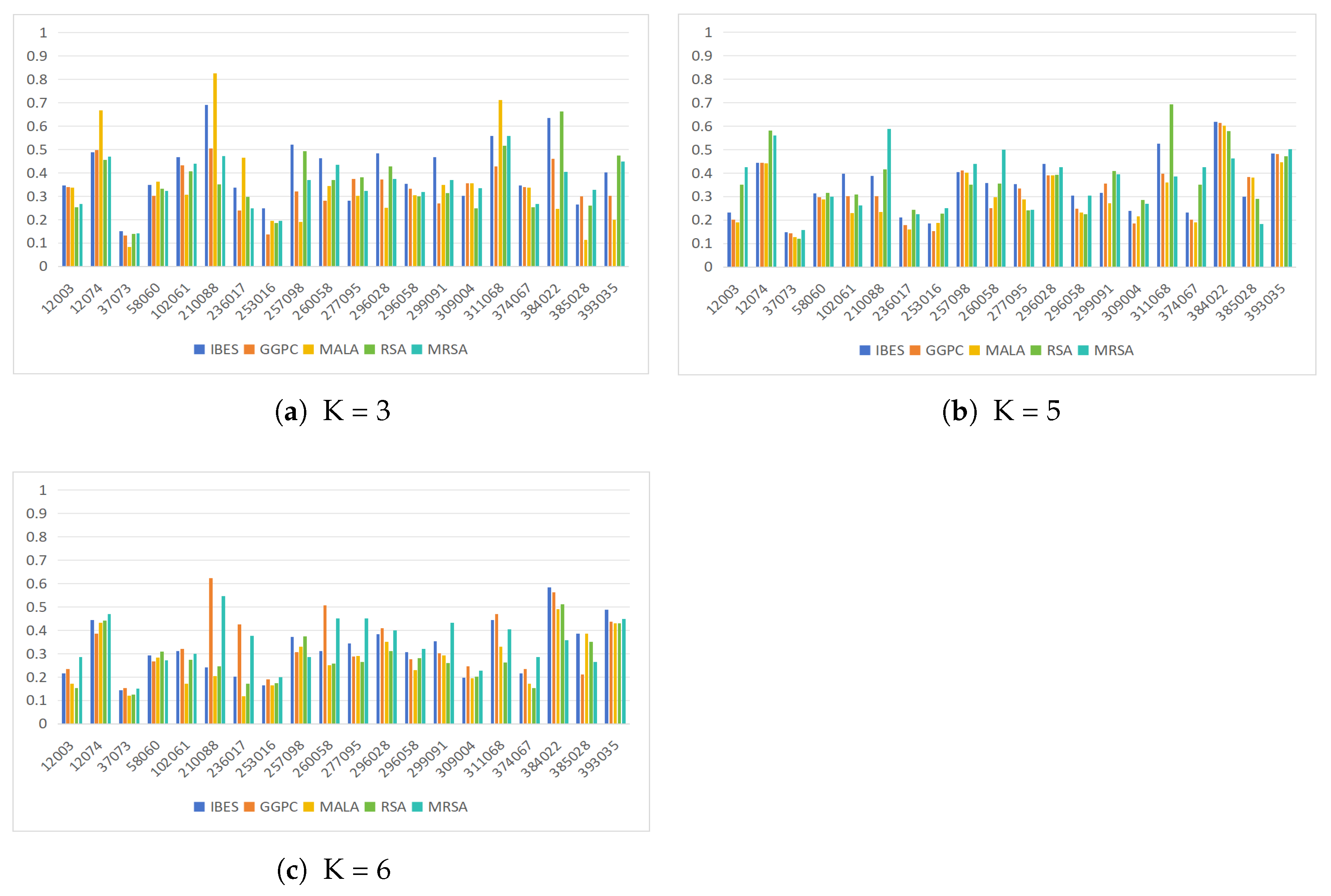
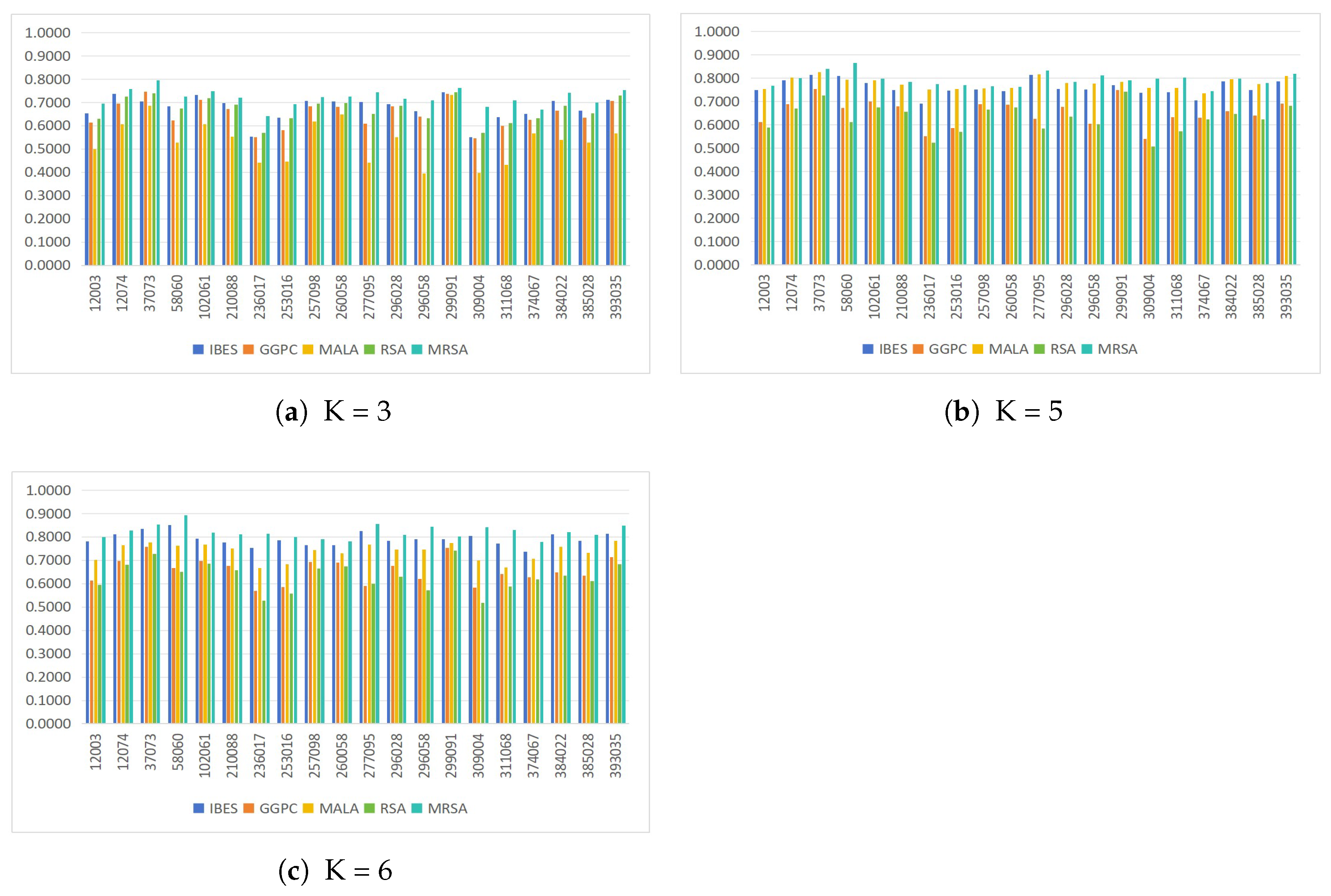
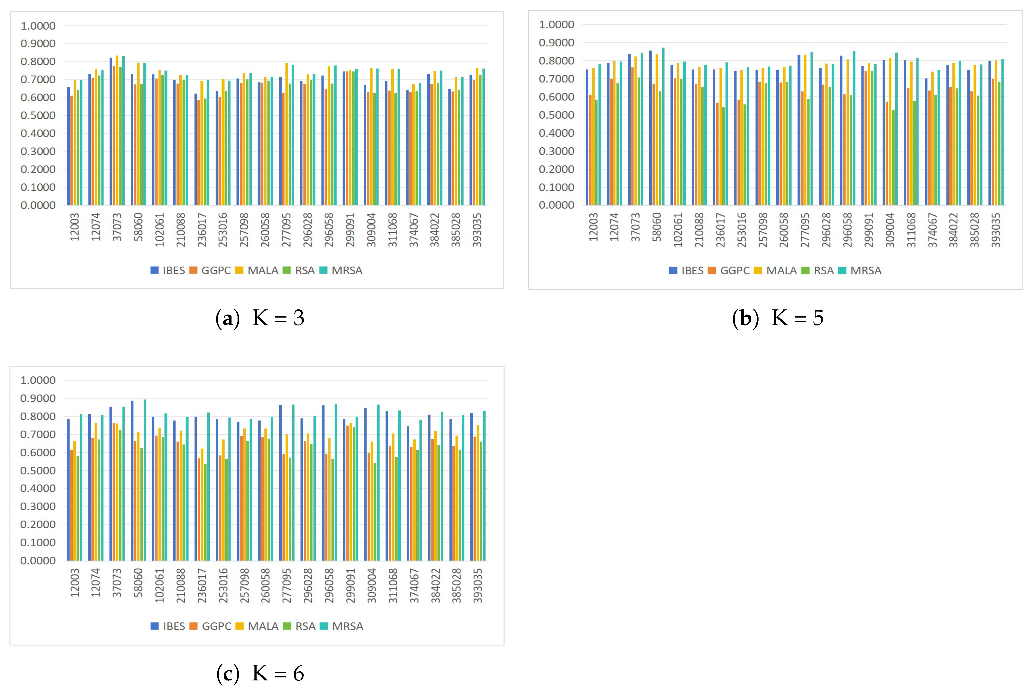
To accurately assess segmentation quality from a perceptual perspective, we utilize RC, a standard evaluation metric for image segmentation. RC measures the overlap between the segmentation results and the human-annotated ground truth. Figure 2 depicts the RC values for all comparison algorithms under the Kapur objective function at three threshold levels.

At the low threshold, there are small differences in the performance of the algorithms. IBES achieves the highest RC values on 10 out of 20 images. MRSA ranks second and obtains the best RC value on “385028”. GGPC, MALA, and RSA show competitive performance on one, five, and three images, respectively. Although MALA outperforms MRSA, the difference is generally marginal. However, MALA performs worst on seven images.

As the number of thresholds increases to five, MRSA achieves the highest RC values on nine images. For images “12003”, “210088”, and “260058”, MRSA demonstrates superior performance compared to other algorithms. Its RC values are 0.4262, 0.5873, and 0.4996, indicating improvements of approximately 21.3%, 41.0%, and 39.5% over the second-best algorithm. At the most challenging threshold level (K = 6), MRSA continues to demonstrate strong performance. It acquires the highest RC values on seven images. Notably, on images “277095”, “299091”, and “393035”, MRSA achieves RC values of 0.4518 and 0.4318, which are substantially higher than those of the comparison algorithms.

4.1.4. Analysis of Other Evaluation Metrics Based on Kapur

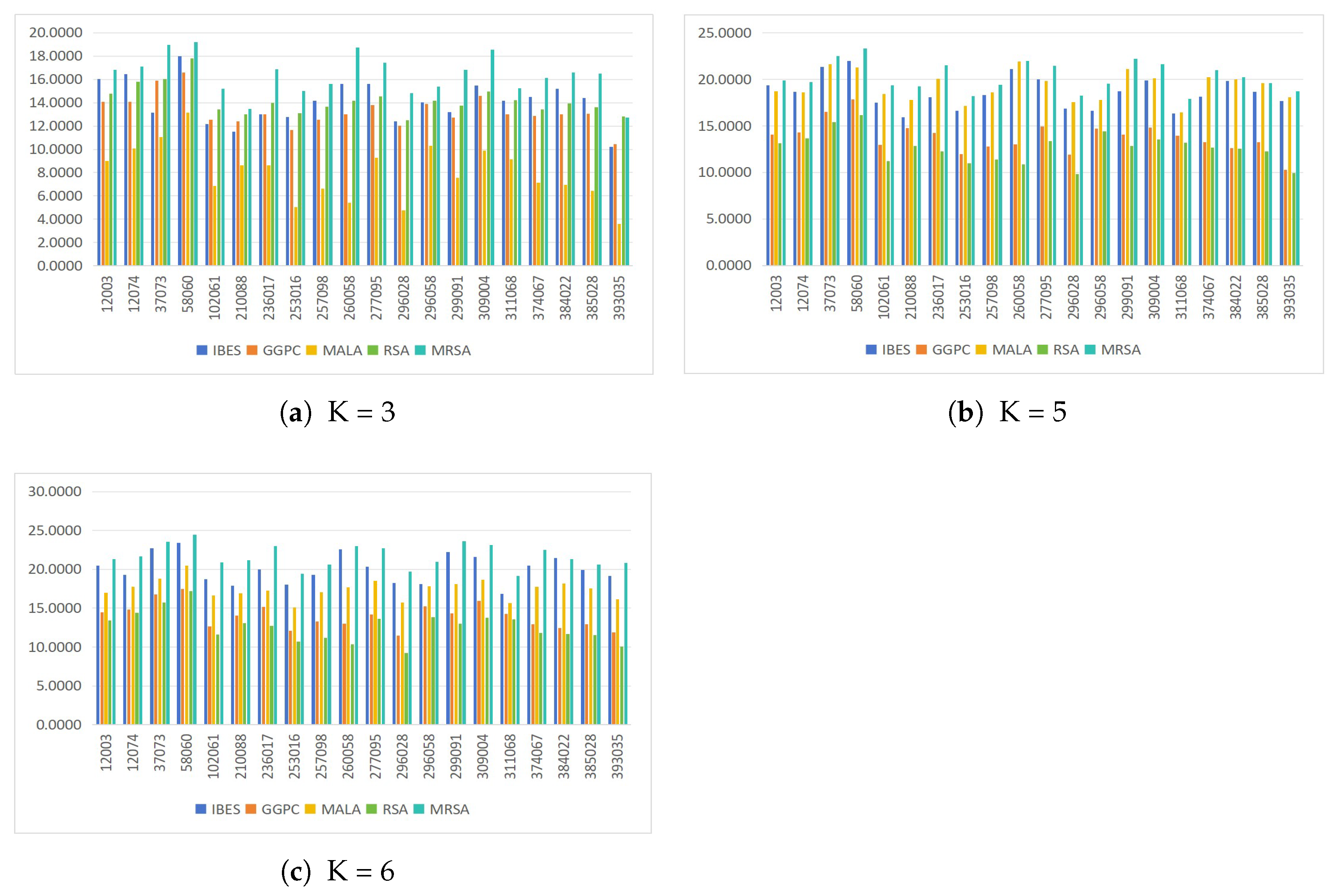
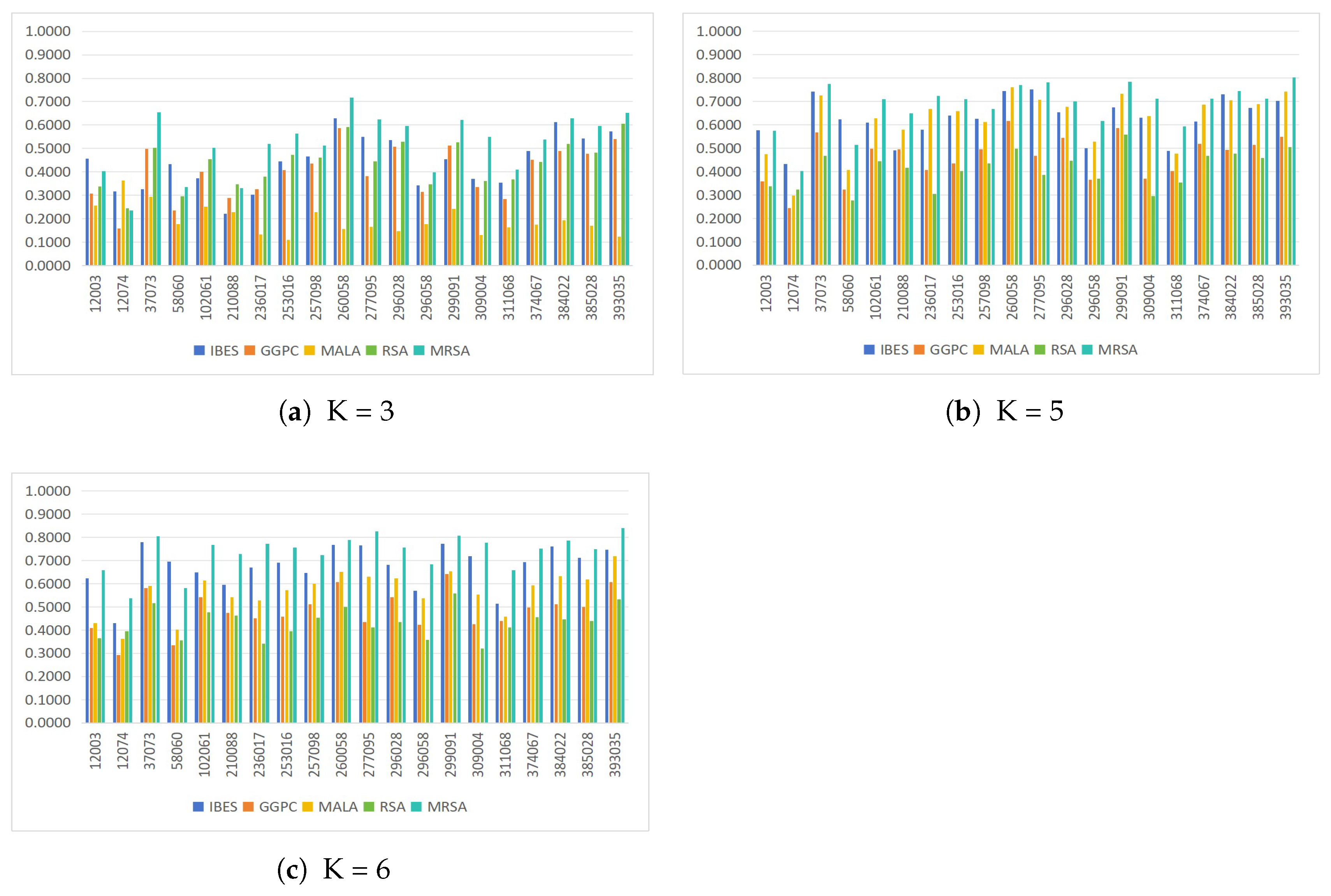
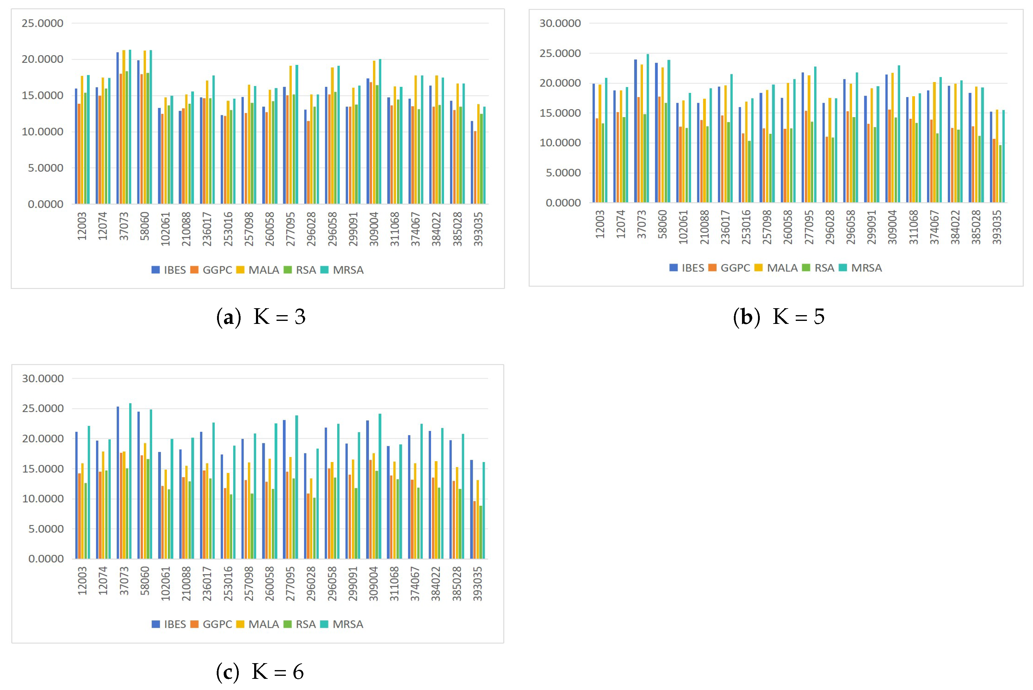
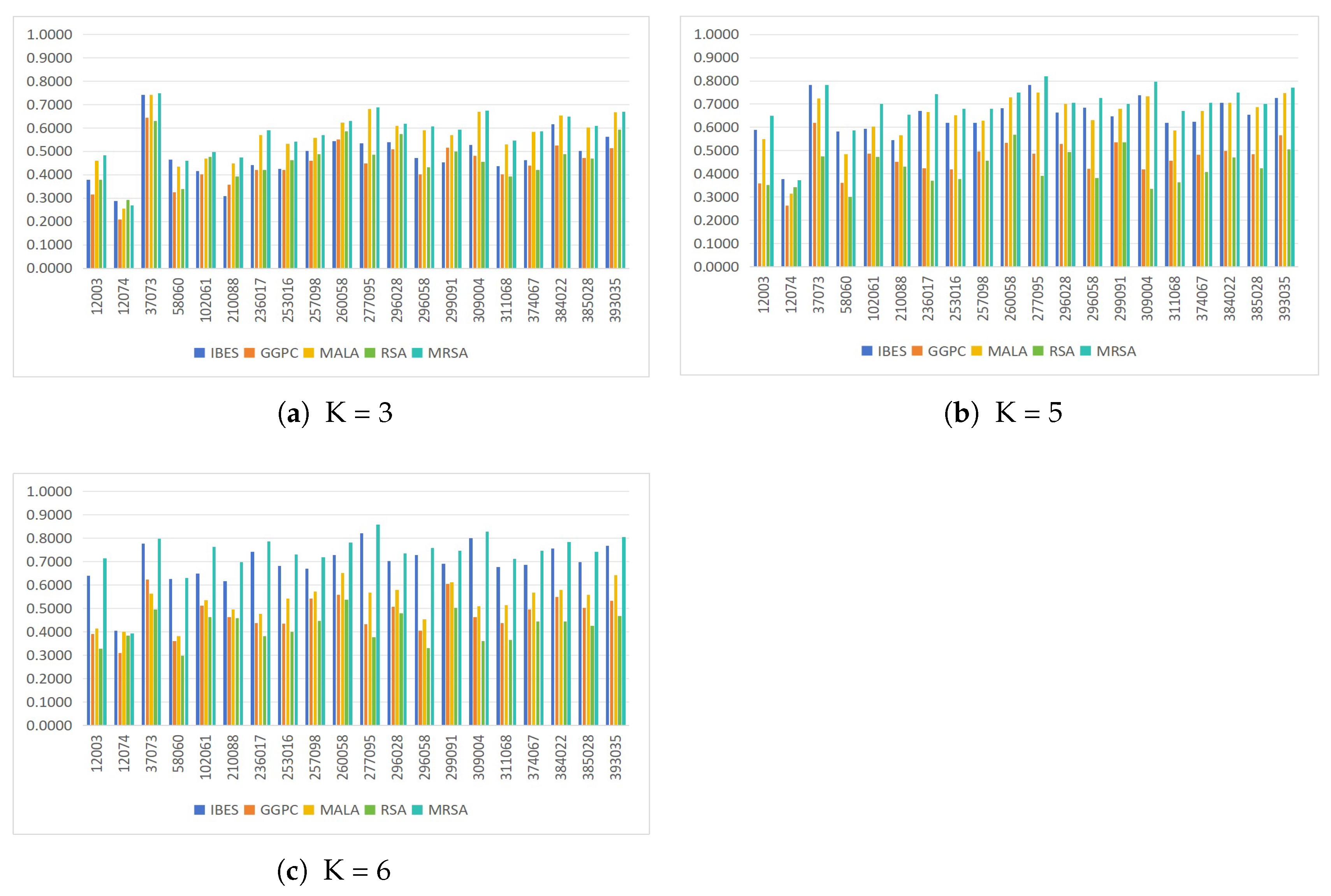
Figure 3, Figure 4 and Figure 5 display the PSNR, SSIM, and FSIM results according to Kapur entropy.

Figure 3 shows that the proposed MRSA algorithm achieves superior segmentation performance on most test color images at different threshold levels. Compared to IBES, GGPC, MALA, and RSA, MRSA obtains higher PSNR values at 57 image-threshold combinations. IBES, MALA, and RSA outperform MRSA on 1, 1, and 1 image segmentation, respectively. The segmented images produced by MRSA better preserve the information of the original images and exhibit higher visual quality.

According to Figure 4, MRSA achieves favorable structural similarity performance at 52 cases, followed by IBES, MALA, GGPC, and RSA. For the lower threshold level, IBES, MALA, and GGPC achieve their best performance with two, one, and one cases, respectively. IBES also outperforms MRSA on three and one cases when K = 5 and 6. Traditional color image segmentation methods usually process the RGB channels independently and ignore the correlations between different color channels. The SSIM results indicate that MRSA can better preserve the structural information and texture details of the original images during multi-threshold color image segmentation.

MRSA achieves the highest FSIM values across different threshold levels, and it performs worse than MALA only on image “12074” when K = 5. MRSA has shown superior performance over other comparison algorithms in feature information preservation and visual perception quality, as evidenced by FSIM experimental results based on the Kapur objective function.

4.2. Comparative Results Based on Otsu Criterion

4.2.1. Analysis of the Objective Function Based on Otsu

Table 6. The objective function values using Otsu.

Level	Image	IBES	GGPC	MALA	RSA	MRSA
		Minimum/Mean/STD	Minimum/Mean/STD	Minimum/Mean/STD	Minimum/Mean/STD	Minimum/Mean/STD
3	12003	2298.01/2314.30/24.57	2282.01/2353.04/32.50	2442.21/2444.92/0.78	2355.62/2409.52/32.06	2384.51/2435.47/14.01
	12074	3054.54/3059.41/14.95	3053.47/3101.45/23.05	3164.59/3164.70/0.04	3054.56/3138.46/29.14	3141.86/3157.32/5.72
	37073	629.23/630.91/4.51	603.29/632.29/14.44	669.55/670.01/0.11	619.87/656.04/14.32	647.76/666.12/6.38
	58060	2073.26/2083.80/17.92	1998.40/2082.93/31.62	2153.25/2154.64/0.40	2073.26/2136.81/27.32	2106.44/2148.11/10.99
	102061	2498.35/2498.40/0.03	2500.03/2550.00/25.90	2628.82/2629.67/0.20	2539.37/2587.66/33.42	2584.97/2620.29/15.36
	210088	1592.51/1592.59/0.04	1570.07/1614.84/23.94	1695.90/1695.95/0.01	1620.34/1665.30/27.47	1629.23/1685.02/15.72
	236017	693.07/693.16/0.04	652.25/690.49/21.23	766.57/766.62/0.02	642.23/725.14/34.58	709.52/754.90/12.71
	253016	1796.27/1882.97/20.41	1801.01/1893.66/49.37	2001.55/2005.08/0.83	1771.86/1960.27/49.40	1935.57/1990.93/12.77
	257098	2972.16/2988.85/23.61	2904.14/2996.77/40.77	3108.21/3113.42/1.33	2890.92/3063.12/58.43	3058.14/3104.67/11.80
	260058	961.45/1005.91/15.20	936.97/986.41/26.75	1075.67/1075.80/0.05	987.27/1037.74/26.07	984.40/1057.25/24.81
	277095	1364.34/1372.82/14.92	1241.08/1353.61/37.69	1462.20/1462.78/0.14	1364.34/1425.09/28.12	1386.50/1450.54/16.90
	296028	2333.06/2506.32/40.78	2446.77/2545.02/43.40	2659.40/2659.47/0.03	1744.24/2566.94/198.26	2630.46/2650.20/8.39
	296058	1334.34/1348.50/23.34	1263.98/1351.94/39.40	1448.29/1448.45/0.05	1334.37/1417.25/35.42	1401.23/1443.37/11.16
	299091	1100.27/1132.16/14.33	1089.03/1139.58/27.90	1230.43/1230.47/0.01	1076.66/1188.73/39.88	1161.68/1217.42/15.20
	309004	668.44/669.64/5.08	617.18/679.56/19.79	741.57/741.67/0.04	661.61/720.02/21.70	669.19/731.90/15.73
	311068	1895.91/1895.94/0.02	1799.46/1895.06/33.13	1966.30/1970.03/1.63	1014.48/1893.23/208.8	1907.74/1964.03/15.06
	374067	1316.98/1317.07/0.04	1246.33/1300.46/28.95	1388.63/1388.71/0.02	681.73/1300.34/159.62	1344.84/1378.5/11.08
	384022	2519.50/2541.29/21.15	2441.66/2527.56/36.83	2625.58/2626.97/0.84	2299.37/2574.16/71.33	2557.00/2611.19/19.51
	385028	1788.85/1788.90/0.03	1742.54/1821.93/34.04	1891.48/1910.60/4.55	1102.93/1812.96/174.68	1818.10/1903.70/25.93
	393035	3115.73/3119.89/18.27	3103.11/3151.60/26.76	3237.35/3237.37/0.005	3063.23/3206.79/44.70	3224.28/3228.39/3.08
5	12003	2485.90/2515.17/6.89	2391.16/2467.77/33.41	2056.06/2477.27/150.82	814.03/1131.79/667.40	2498.87/2538.32/13.69
	12074	3172.98/3215.65/10.70	3155.46/3185.68/13.09	2523.16/3178.11/157.97	1012.98/1308.76/719.62	3205.88/3230.34/9.77
	37073	683.59/689.12/2.32	644.49/664.23/10.19	403.61/670.23/66.36	183.06/242.53/164.34	685.40/695.17/5.67
	58060	2211.51/2212.13/1.42	2106.58/2169.16/20.30	964.91/2053.99/358.15	976.08/1257.07/648.79	2201.23/2224.35/7.35
	102061	2672.15/2694.62/6.73	2590.65/2651.82/21.93	1558.78/2580.42/348.23	503.68/1407.24/561.46	2677.88/2708.63/14.32
	210088	1714.97/1734.55/9.53	1667.21/1705.27/19.71	951.58/1667.07/224.29	520.16/612.14/339.78	1722.79/1755.70/11.59
	236017	755.98/797.63/12.11	712.04/748.17/16.38	656.09/797.12/39.50	259.30/459.73/195.57	755.69/806.71/11.13
	253016	2023.38/2052.53/13.29	1960.39/2008.45/21.67	1257.30/1929.53/284.28	824.00/1011.76/514.40	2023.47/2067.53/17.94
	257098	3159.13/3179.19/9.38	3057.43/3121.39/28.83	2245.42/3054.92/349.6	958.97/1289.07/692.03	3162.94/3200.82/14.49
	260058	1087.35/1106.89/6.13	1024.73/1055.21/21.02	1014.68/1099.12/25.70	374.80/550.09/243.65	1073.76/1108.00/11.45
	277095	1491.23/1508.61/4.49	1401.80/1444.73/20.46	1010.70/1473.48/122.48	381.29/610.81/361.09	1492.73/1520.28/10.07
	296028	2684.89/2711.69/11.52	2617.55/2665.05/21.40	1580.04/2676.46/258.37	1093.37/1325.57/605.46	2696.59/2726.63/12.57
	296058	1489.37/1503.11/8.54	1377.82/1451.20/26.80	546.42/1414.11/259.13	517.67/700.97/434.17	1445.25/1522.70/19.32
	299091	1260.84/1271.54/5.43	1148.75/1206.21/29.57	1220.00/1282.66/18.33	405.53/660.20/366.32	1248.82/1280.18/9.30
	309004	765.29/778.59/5.49	674.51/736.80/24.08	633.21/775.86/44.51	255.88/344.07/185.75	769.23/788.03/8.81
	311068	1982.92/2004.76/7.22	1905.58/1964.65/20.19	1893.14/1995.29/34.81	922.17/1121.36/520.32	1987.58/2013.08/12.33
	374067	1406.65/1427.83/7.71	1353.41/1384.52/13.49	1340.82/1436.07/27.16	463.19/576.14/258.58	1420.03/1430.70/8.30
	384022	2670.23/2685.35/6.99	2620.79/2649.67/15.74	1693.01/2608.90/279.64	780.39/906.53/460.29	2685.48/2702.30/8.30
	385028	1956.47/1981.16/8.60	1858.80/1927.08/28.05	1186.41/1928.51/220.06	567.40/716.47/383.11	1945.53/1989.79/12.37
	393035	3271.90/3283.12/3.84	3209.10/3249.31/18.03	2136.76/3229.94/261.18	1141.51/1454.94/685.86	3278.35/3294.11/6.62
6	12003	2538.03/2550.39/7.10	2449.20/2500.25/21.30	1190.56/1485.21/624.16	291.58/419.76/134.16	2527.42/2560.60/10.27
	12074	3235.85/3242.37/3.14	3172.52/3207.17/12.17	1975.11/2398.35/798.19	501.57/682.61/251.42	3228.05/3246.43/7.60
	37073	696.72/701.56/1.98	660.23/676.29/8.17	262.38/330.88/139.17	73.11/81.36/4.44	697.35/701.45/2.84
	58060	2227.41/2234.42/2.22	2158.16/2199.12/16.89	824.06/1145.00/551.82	389.77/430.37/112.37	2224.07/2238.95/5.87
	102061	2706.67/2721.36/8.55	2636.15/2672.43/20.25	1411.81/1743.64/628.05	411.60/498.67/190.70	2704.68/2732.75/12.46
	210088	1746.26/1764.12/9.40	1693.23/1725.12/13.65	967.61/1194.97/434.58	218.49/263.90/113.31	1745.89/1768.29/9.39
	236017	811.82/820.44/4.39	741.10/775.05/20.02	237.95/408.32/193.76	67.30/78.91/24.56	772.51/818.61/10.36
	253016	2080.74/2090.82/5.45	1994.69/2038.95/21.51	1081.51/1284.31/312.13	422.55/509.05/226.24	2042.12/2089.59/14.22
	257098	3186.19/3215.45/10.44	3144.98/3174.25/19.08	1596.42/1979.27/889.01	317.59/408.04/208.69	3193.79/3222.82/12.12
	260058	1111.27/1122.63/5.63	1019.93/1078.44/21.37	580.44/705.66/252.81	163.96/175.80/26.56	1079.70/1123.18/12.01
	277095	1525.38/1533.39/2.66	1428.78/1476.04/21.31	534.34/718.89/386.76	181.26/311.45/196.04	1522.77/1534.86/6.05
	296028	2658.74/2739.19/21.12	2633.24/2687.77/23.95	1094.42/1377.6/513.32	364.39/400.84/145.05	2724.89/2745.66/10.70
	296058	1509.64/1533.48/6.76	1463.76/1483.54/13.86	707.09/865.69/358.33	219.96/242.80/69.49	1502.76/1535.25/12.71
	299091	1272.80/1293.52/6.34	1213.85/1244.21/15.89	609.69/783.02/361.57	212.01/304.83/145.75	1268.02/1296.03/8.20
	309004	785.74/802.57/5.45	733.38/760.92/13.21	321.83/469.89/202.91	98.81/139.27/94.58	777.64/803.00/8.23
	311068	2008.42/2022.35/5.93	1959.36/1987.99/11.48	1054.68/1293.47/538.31	302.38/369.03/121.55	2015.23/2025.50/6.01
	374067	1446.68/1451.94/4.82	1367.27/1402.68/20.47	591.60/734.80/401.57	130.13/163.89/58.01	1422.51/1452.91/9.18
	384022	2710.64/2722.42/5.56	2625.54/2674.24/18.86	1256.35/1536.31/611.81	514.93/659.07/266.58	2702.60/2727.77/10.39
	385028	2004.13/2013.07/4.46	1912.27/1951.17/19.69	941.38/1199.52/479.52	348.20/430.93/114.07	1977.99/2014.59/11.60
	393035	3291.12/3306.38/5.57	3234.18/3267.28/16.40	1840.56/2229.53/837.20	32.74/395.25/157.34	3292.68/3306.79/9.07

reports the objective function results using Otsu. MRSA demonstrates strong optimization capability and stability at different threshold levels. The Otsu objective values of the algorithms generally increase as the number of thresholds increases. By using more thresholds, it is possible to maximize the between-class variance among different image regions and produce more detailed segmentation outcomes.

At the lower threshold level, the performance differences among the algorithms are relatively small. Because the low-dimensional search space is less complex, most algorithms quickly converge to promising regions. RSA, MALA, and MRSA achieve high Otsu values, with MALA even performing slightly better than MRSA in some cases. When the thresholds increase to five, MRSA’s advantages become more apparent, while the performance of MALA and RSA experience fluctuations. Except for images “299091” and “374067”, MRSA achieves the best Otsu values. As the search space dimension increases, GGPC and RSA are more likely to fall into local optima due to insufficient population diversity. In contrast, MRSA introduces an adaptive weight mechanism to achieve a dynamic balance between exploration and exploitation. In the higher-dimensional threshold segmentation task, the performance of MRSA is superior to other algorithms. GGPC and RSA show a clear decline in optimization capability and large fluctuations in high-dimensional search spaces, while MRSA still maintains stable and high Otsu values.

Table 7. Wilcoxon rank-sum test on objective function values.

Level	Image	IBES	GGPC	MALA	RSA	MRSA
3	12003	6.07 $\times {10}^{-8}$	6.43 $\times {10}^{-8}$	-	3.12 $\times {10}^{-5}$	6.43 $\times {10}^{-8}$
	12074	6.32 $\times {10}^{-8}$	6.63 $\times {10}^{-8}$	-	6.12 $\times {10}^{-6}$	6.63 $\times {10}^{-8}$
	37073	4.89 $\times {10}^{-8}$	5.61 $\times {10}^{-8}$	-	2.64 $\times {10}^{-6}$	5.61 $\times {10}^{-8}$
	58060	6.64 $\times {10}^{-8}$	6.70 $\times {10}^{-8}$	-	2.33 $\times {10}^{-3}$	6.70 $\times {10}^{-8}$
	102061	4.07 $\times {10}^{-8}$	4.49 $\times {10}^{-8}$	-	4.61 $\times {10}^{-6}$	4.49 $\times {10}^{-8}$
	210088	4.27 $\times {10}^{-8}$	4.46 $\times {10}^{-8}$	-	1.41 $\times {10}^{-5}$	4.46 $\times {10}^{-8}$
	236017	5.72 $\times {10}^{-8}$	6.09 $\times {10}^{-8}$	-	1.03 $\times {10}^{-7}$	6.09 $\times {10}^{-8}$
	253016	5.82 $\times {10}^{-8}$	6.24 $\times {10}^{-8}$	-	1.80 $\times {10}^{-6}$	6.24 $\times {10}^{-8}$
	257098	5.23 $\times {10}^{-8}$	5.33 $\times {10}^{-8}$	-	2.54 $\times {10}^{-5}$	8.42 $\times {10}^{-8}$
	260058	5.04 $\times {10}^{-8}$	5.35 $\times {10}^{-8}$	-	4.95 $\times {10}^{-6}$	5.35 $\times {10}^{-8}$
	277095	3.37 $\times {10}^{-8}$	3.47 $\times {10}^{-8}$	-	1.17 $\times {10}^{-7}$	3.47 $\times {10}^{-8}$
	296028	4.97 $\times {10}^{-8}$	5.33 $\times {10}^{-8}$	-	2.75 $\times {10}^{-6}$	5.33 $\times {10}^{-8}$
	296058	5.77 $\times {10}^{-8}$	6.00 $\times {10}^{-8}$	-	1.14 $\times {10}^{-3}$	6.00 $\times {10}^{-8}$
	299091	3.33 $\times {10}^{-8}$	3.47 $\times {10}^{-8}$	-	1.23 $\times {10}^{-6}$	3.47 $\times {10}^{-8}$
	309004	4.77 $\times {10}^{-8}$	4.94 $\times {10}^{-8}$	-	1.66 $\times {10}^{-5}$	4.94 $\times {10}^{-8}$
	311068	5.37 $\times {10}^{-8}$	5.71 $\times {10}^{-8}$	-	9.17 $\times {10}^{-6}$	8.99 $\times {10}^{-8}$
	374067	3.76 $\times {10}^{-8}$	3.99 $\times {10}^{-8}$	-	4.86 $\times {10}^{-7}$	3.99 $\times {10}^{-8}$
	384022	5.67 $\times {10}^{-8}$	5.72 $\times {10}^{-8}$	-	1.86 $\times {10}^{-5}$	1.41 $\times {10}^{-7}$
	385028	3.10 $\times {10}^{-8}$	4.06 $\times {10}^{-8}$	-	1.61 $\times {10}^{-7}$	1.03 $\times {10}^{-7}$
	393035	2.26 $\times {10}^{-8}$	2.44 $\times {10}^{-8}$	-	1.18 $\times {10}^{-5}$	2.44 $\times {10}^{-8}$
5	12003	1.99 $\times {10}^{-1}$	1.20 $\times {10}^{-6}$	1.40 $\times {10}^{-1}$	6.80 $\times {10}^{-8}$	-
	12074	5.50 $\times {10}^{-4}$	1.06 $\times {10}^{-7}$	9.03 $\times {10}^{-1}$	6.70 $\times {10}^{-8}$	-
	37073	8.07 $\times {10}^{-3}$	6.80 $\times {10}^{-8}$	2.80 $\times {10}^{-3}$	1.22 $\times {10}^{-7}$	-
	58060	4.35 $\times {10}^{-5}$	7.90 $\times {10}^{-8}$	2.18 $\times {10}^{-1}$	3.07 $\times {10}^{-6}$	-
	102061	3.32 $\times {10}^{-3}$	1.23 $\times {10}^{-7}$	5.25 $\times {10}^{-1}$	6.79 $\times {10}^{-8}$	-
	210088	2.79 $\times {10}^{-3}$	3.94 $\times {10}^{-7}$	7.64 $\times {10}^{-2}$	6.78 $\times {10}^{-8}$	-
	236017	4.59 $\times {10}^{-4}$	5.23 $\times {10}^{-7}$	1.79 $\times {10}^{-4}$	1.57 $\times {10}^{-6}$	-
	253016	2.98 $\times {10}^{-1}$	1.38 $\times {10}^{-6}$	5.25 $\times {10}^{-1}$	6.75 $\times {10}^{-8}$	-
	257098	1.37 $\times {10}^{-6}$	7.90 $\times {10}^{-8}$	1.00 $\times {10}^0$	6.75 $\times {10}^{-8}$	-
	260058	9.05 $\times {10}^{-3}$	6.01 $\times {10}^{-7}$	2.08 $\times {10}^{-1}$	6.80 $\times {10}^{-8}$	-
	277095	6.51 $\times {10}^{-3}$	6.80 $\times {10}^{-8}$	6.36 $\times {10}^{-1}$	6.70 $\times {10}^{-8}$	-
	296028	1.48 $\times {10}^{-1}$	7.90 $\times {10}^{-8}$	1.95 $\times {10}^{-3}$	6.76 $\times {10}^{-8}$	-
	296058	5.30 $\times {10}^{-2}$	5.23 $\times {10}^{-7}$	3.94 $\times {10}^{-1}$	1.04 $\times {10}^{-6}$	-
	299091	1.47 $\times {10}^{-3}$	2.56 $\times {10}^{-7}$	-	9.16 $\times {10}^{-8}$	4.17 $\times {10}^{-5}$
	309004	9.04 $\times {10}^{-3}$	7.90 $\times {10}^{-8}$	1.08 $\times {10}^{-1}$	3.93 $\times {10}^{-7}$	-
	311068	7.15 $\times {10}^{-1}$	1.06 $\times {10}^{-7}$	6.75 $\times {10}^{-1}$	1.91 $\times {10}^{-7}$	-
	374067	1.95 $\times {10}^{-3}$	3.50 $\times {10}^{-6}$	-	9.16 $\times {10}^{-8}$	1.20 $\times {10}^{-1}$
	384022	1.58 $\times {10}^{-6}$	6.80 $\times {10}^{-8}$	5.61 $\times {10}^{-1}$	6.47 $\times {10}^{-8}$	-
	385028	7.15 $\times {10}^{-1}$	2.96 $\times {10}^{-7}$	1.35 $\times {10}^{-3}$	6.77 $\times {10}^{-8}$	-
	393035	9.04 $\times {10}^{-7}$	6.80 $\times {10}^{-8}$	9.03 $\times {10}^{-1}$	7.85 $\times {10}^{-8}$	-
6	12003	1.90 $\times {10}^{-1}$	6.80 $\times {10}^{-8}$	6.79 $\times {10}^{-8}$	4.95 $\times {10}^{-8}$	-
	12074	7.76 $\times {10}^{-1}$	6.80 $\times {10}^{-8}$	1.23 $\times {10}^{-7}$	4.95 $\times {10}^{-8}$	-
	37073	-	6.79 $\times {10}^{-8}$	6.79 $\times {10}^{-8}$	3.47 $\times {10}^{-8}$	1.81 $\times {10}^{-1}$
	58060	1.90 $\times {10}^{-1}$	6.80 $\times {10}^{-8}$	6.80 $\times {10}^{-8}$	9.65 $\times {10}^{-8}$	-
	102061	3.60 $\times {10}^{-2}$	9.17 $\times {10}^{-8}$	6.80 $\times {10}^{-8}$	4.95 $\times {10}^{-8}$	-
	210088	7.35 $\times {10}^{-1}$	6.80 $\times {10}^{-8}$	4.54 $\times {10}^{-7}$	4.49 $\times {10}^{-8}$	-
	236017	-	7.90 $\times {10}^{-8}$	6.80 $\times {10}^{-8}$	3.48 $\times {10}^{-8}$	7.95 $\times {10}^{-7}$
	253016	-	6.80 $\times {10}^{-8}$	6.80 $\times {10}^{-8}$	1.72 $\times {10}^{-7}$	1.12 $\times {10}^{-3}$
	257098	2.14 $\times {10}^{-3}$	1.66 $\times {10}^{-7}$	1.23 $\times {10}^{-7}$	3.48 $\times {10}^{-8}$	-
	260058	3.75 $\times {10}^{-4}$	1.80 $\times {10}^{-6}$	6.01 $\times {10}^{-7}$	5.37 $\times {10}^{-8}$	-
	277095	1.14 $\times {10}^{-1}$	6.80 $\times {10}^{-8}$	6.79 $\times {10}^{-8}$	5.37 $\times {10}^{-8}$	-
	296028	4.09 $\times {10}^{-1}$	6.80 $\times {10}^{-8}$	6.76 $\times {10}^{-8}$	4.00 $\times {10}^{-8}$	-
	296058	1.44 $\times {10}^{-2}$	1.66 $\times {10}^{-7}$	7.94 $\times {10}^{-7}$	6.03 $\times {10}^{-8}$	-
	299091	8.60 $\times {10}^{-6}$	2.22 $\times {10}^{-7}$	2.36 $\times {10}^{-6}$	5.73 $\times {10}^{-8}$	-
	309004	1.23 $\times {10}^{-3}$	1.43 $\times {10}^{-7}$	9.17 $\times {10}^{-8}$	4.95 $\times {10}^{-8}$	-
	311068	2.62 $\times {10}^{-1}$	6.80 $\times {10}^{-8}$	1.05 $\times {10}^{-6}$	6.03 $\times {10}^{-8}$	-
	374067	3.85 $\times {10}^{-2}$	1.92 $\times {10}^{-7}$	1.23 $\times {10}^{-7}$	4.00 $\times {10}^{-8}$	-
	384022	1.40 $\times {10}^{-1}$	6.80 $\times {10}^{-8}$	6.80 $\times {10}^{-8}$	6.28 $\times {10}^{-8}$	-
	385028	8.36 $\times {10}^{-4}$	6.80 $\times {10}^{-8}$	6.80 $\times {10}^{-8}$	5.73 $\times {10}^{-8}$	-
	393035	6.56 $\times {10}^{-3}$	1.06 $\times {10}^{-7}$	9.17 $\times {10}^{-8}$	4.00 $\times {10}^{-8}$	-

presents the Wilcoxon rank-sum test of the algorithms on objective function values. When K = 3, MALA achieves the best results on all test images, while the other algorithms are inferior to it. When K increases to 5, the statistical advantage of MRSA is more apparent. MRSA achieves the best performance on 18 out of 20 images. It is important to note that IBES and MALA achieve results comparable to MRSA on several images, including “12003”, “58060”, “253016”, and “277095”. In the higher-dimensional multi-threshold segmentation task (K = 6), MRSA achieves “-” at 17 images, while the other algorithms exhibit no statistical similar to it. In images “257098”, “296058”, “311068”, and “384022”, MRSA and IBES achieve comparable results. GGPC and RSA demonstrate relatively weak performance under different threshold levels.

The Friedman test results show that the average ranks for IBES, GGPC, MALA, RSA, and MRSA are 3.17, 3.25, 2.42, 4.58, and 1.58, respectively, with a p-value of 1.03E-24. MRSA performs the best, followed by MALA, IBES, GGPC, and RSA. Wilcoxon rank-sum and Friedman tests demonstrate that MRSA has significant statistical advantages in medium- and high-dimensional multi-threshold color image segmentation tasks.

4.2.2. Analysis of the Running Time Based on Otsu

Table 8. The average running time.

Level	Image	IBES	GGPC	MALA	RSA	MRSA
3	12003	2.8116	3.0241	2.8568	2.8927	6.8275
	12074	2.7772	2.9289	2.8093	2.8629	6.6806
	37073	2.6995	3.0103	2.7558	2.8357	6.6476
	58060	2.7979	3.0390	2.8116	2.8765	6.6711
	102061	2.7468	2.9880	2.7792	2.8101	6.6631
	210088	2.7759	3.0110	2.8039	2.8536	6.6061
	236017	2.7582	3.0442	2.7696	2.8183	6.6570
	253016	2.7335	2.9437	2.7607	2.7795	6.7341
	257098	2.7340	2.9737	2.7167	2.7935	6.5853
	260058	2.7382	3.0272	2.7402	2.7541	6.6303
	277095	2.7586	2.9826	2.7660	2.8084	6.5678
	296028	2.7316	2.9676	2.7450	2.7797	6.6778
	296058	2.7466	3.0319	2.7518	2.8137	6.6331
	299091	2.7168	2.9959	2.7443	2.8116	6.6358
	309004	2.7598	2.9864	2.7842	2.8349	6.6735
	311068	2.7542	2.9759	2.7808	2.8212	6.5996
	374067	2.7341	2.9734	2.7609	2.8165	6.5680
	384022	2.7563	3.0023	2.7725	2.8519	6.6374
	385028	2.7281	3.0310	2.7447	2.7977	6.6617
	393035	2.7181	2.9052	2.7394	2.7955	6.5604
5	12003	3.9065	4.3396	3.9692	4.2468	7.1203
	12074	3.8181	4.1843	3.9402	4.1644	6.8824
	37073	3.7291	4.6397	3.9041	4.4213	6.8944
	58060	3.8356	4.3132	3.9274	4.1401	6.9017
	102061	3.7683	4.3399	3.9090	4.2340	6.8677
	210088	3.8205	4.4445	3.9351	4.2882	6.8610
	236017	3.7070	4.4559	3.7798	4.1828	6.8614
	253016	3.6905	4.2841	3.7177	4.1466	6.9620
	257098	3.6952	4.3575	3.7691	4.1950	6.7684
	260058	3.6746	4.2850	3.6388	4.0351	6.8556
	277095	3.7118	4.4699	3.8590	4.2997	6.7835
	296028	3.6905	4.3094	3.7574	4.1248	6.8955
	296058	3.7073	4.4973	3.8238	4.2762	6.8281
	299091	3.7135	4.4425	3.7912	4.2207	6.8469
	309004	3.7653	4.5346	3.8374	4.2129	6.9224
	311068	3.7684	4.3549	3.8757	4.1634	6.8013
	374067	3.7227	4.3737	3.8289	4.3325	6.7906
	384022	3.7690	4.4029	3.8670	4.3408	6.8612
	385028	3.6895	4.3764	3.7611	4.2309	6.8555
	393035	3.6604	4.0950	3.7348	3.9933	6.7770
6	12003	4.6736	5.2905	5.1586	5.2165	7.3220
	12074	4.6676	5.1991	5.2297	5.2083	7.0229
	37073	4.5524	5.5726	5.4036	5.4637	7.0514
	58060	4.6797	5.2812	5.2858	5.1933	7.0643
	102061	4.5676	5.3042	5.1968	5.3908	7.0206
	210088	4.6408	5.5263	5.3257	5.5414	6.9970
	236017	4.4609	5.5097	5.0540	5.3434	6.9780
	253016	4.4480	5.1828	5.1600	4.9738	7.0964
	257098	4.4435	5.3046	6.1233	5.3615	6.9283
	260058	4.3663	5.2146	5.4443	5.0845	6.9952
	277095	4.4937	5.5521	5.7040	5.4758	6.9617
	296028	4.4930	5.1672	5.4302	5.0575	7.0521
	296058	4.5114	5.3814	5.5070	5.3920	6.9664
	299091	4.4743	5.4738	5.4450	5.3219	7.0154
	309004	4.5680	5.4661	5.5302	5.4218	7.0910
	311068	4.5646	5.3270	5.5432	5.2753	6.9733
	374067	4.4819	5.3405	5.5662	5.4058	6.9612
	384022	4.5200	5.3059	5.5716	5.2871	7.0403
	385028	4.4475	5.4294	5.8085	5.2805	7.0243
	393035	4.3683	4.8767	5.3300	4.8120	6.9571

displays the average running time of the algorithms. The overall runtime distribution of the algorithms is similar to that under the Kapur objective function. Among them, MRSA still requires the longest runtime, while MALA, IBES, RSA, and GGPC execute faster.

MRSA runs in about 6.6 and 6.8 s at lower threshold levels, while the other algorithms usually run in around 2.7 and 3.0 s. Compared to the Kapur objective function, the overall runtime of all algorithms is slightly shorter. The computation of Otsu’s between-class variance is relatively simple, which results in less time required for fitness evaluation. The runtime of all algorithms increases as the number of thresholds increases. The proposed improvement strategies introduce additional computational costs, but the overall algorithm structure remains stable and scalable.

The runtime experimental results based on the Otsu objective function indicate that although MRSA is less efficient in terms of computation time compared with the other algorithms, it significantly improves image segmentation quality through multiple optimization strategies. Overall, MRSA achieves a more reasonable balance between computational cost and segmentation performance.

4.2.3. Analysis of the Region Covering Based on Otsu

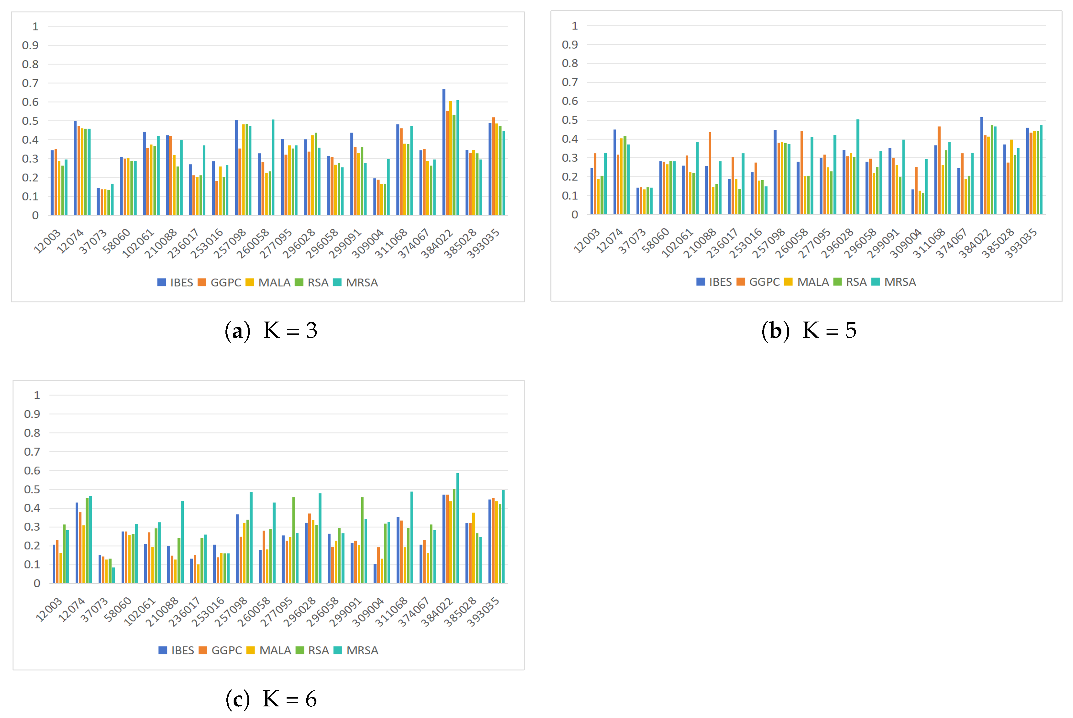
Figure 6 presents the RC results obtained using the Otsu objective function, and it offers evidence of the perceptual quality of the segmentation outcomes produced by the algorithms. At the low threshold level, IBES demonstrates competitive performance, and it achieves the highest RC values on 11 out of 20 images. MRSA obtains outstanding performance on images “37073”, “236017”, “260058”, and “309004”. On “260058”, MRSA outperforms the second-best algorithm (IBES) by approximately 54.9%. On “309004”, MRSA achieves a 52.2% improvement over IBES. GGPC, MALA, and RSA also show great performance at this threshold level, and they achieve the highest RC values on 3, 1, and 1 images, respectively.

With five thresholds, MRSA exhibits significantly improved performance, and it achieves the highest RC values on 10 images. This represents a substantial improvement compared to its performance at K = 3. MRSA achieves notably high RC values on images “257098” (0.4854), “296028” (0.4786), “311068” (0.4887), “384022” (0.5864), and “393035” (0.4962). RSA shows strong performance on several images, particularly “12003”, “277095”, “296058”, “299091”, and “374067”. However, GGPC’s performance is less consistent across all test images. IBES, which performs well at K = 3, experiences a decline in performance at K = 5. For example, IBES’s RC on “384022” decreases from 0.5148 (K = 3) to 0.4706 (K = 5). MALA and RSA exhibit the most significant performance fluctuations. The RC values for RSA on 14 images are significantly lower than those for MRSA.

The superior performance of MRSA at K = 6 is particularly noteworthy because high-dimensional threshold optimization represents the most challenging scenario for metaheuristic algorithms. The search space grows exponentially with the number of thresholds, and many algorithms suffer from insufficient population diversity and premature convergence. RSA exhibits the most significant performance degradation at K = 6. The RC values decline significantly on many images, such as from 0.3129 on “12003” at K = 5 to 0.3129 at K = 6. Through the improvement measures, MRSA explores the high-dimensional search space thoroughly and identifies globally optimal threshold combinations.

4.2.4. Analysis of Other Evaluation Metrics Based on Otsu

Figure 7, Figure 8 and Figure 9 display the PSNR, SSIM, and FSIM results according to the Otsu criterion.

The PSNR experimental results under the Otsu objective function further validate the effectiveness of the proposed algorithm. MRSA achieves the highest PSNR values at 49 images, and it exhibits strong optimization capability in multi-threshold color image segmentation. When K = 3, GGPC shows competitiveness due to its local exploitation ability, and it acquires the best values at six images. Even so, MRSA still achieves superior overall performance. As the number of thresholds increases, MRSA becomes more superior. The PSNR experimental results based on the Otsu objective function demonstrate that MRSA surpasses the comparison algorithms in terms of image reconstruction quality and optimization stability, and it achieves higher-quality segmentation results in complex high-dimensional multi-threshold color image segmentation tasks.

Regarding SSIM, the performance differences among the algorithms are relatively small at the lower threshold level. Even so, MRSA demonstrates clear advantages in complex images. For example, on images “12003” and “37073”, MRSA achieves SSIM values of 0.4837 and 0.7500, respectively, both of which are better than those of the other comparison algorithms. Although MALA shows strong local exploitation ability in low-dimension, its performance fluctuates significantly as the threshold dimension increases. In higher-dimensional multi-threshold segmentation tasks, the SSIM values of RSA and GGPC decrease noticeably, whereas MRSA obtains high performance. These results prove that MRSA has stronger global search capability and greater stability in high-dimensional search spaces.

MRSA achieves high FSIM values at 43 images with various threshold values. At the lower threshold level, MALA shows strong competitiveness, and it surpasses MRSA on 12 cases. However, MRSA exhibits more stable performance. MRSA obtains high-quality results while MALA experiences a significant drop in their FSIM values during higher-dimensional multi-threshold segmentation tasks. The FSIM experimental results based on the Otsu objective function confirm the superior performance of MRSA in multi-threshold color image segmentation.

4.3. Parameter Sensitivity Analysis

To investigate the influence of the number of elite individuals and the weight factor w on the performance of the proposed algorithm, we conduct a sensitivity analysis. The number of elite individuals is set to 4, 5, 7, and 10, respectively, and we record how many times each configuration successfully found the optimal objective function value. The experimental results are presented in

Table 9. The results of different elite individuals based on Kapur.

Level	4	5	7	10
3	3	4	6	7
5	7	5	4	4
6	12	4	2	2

and

Table 10. The results of different elite individuals based on Otsu.

Level	4	5	7	10
3	4	4	6	6
5	8	4	4	4
6	13	3	2	2

.

According to the statistical results based on Kapur, the number of best results generally increases as the number of elite individuals increases when the threshold level is three. In total, 7 and 10 elite individuals achieve 6 and 7 optimal objective function values, respectively. However, when the threshold level increases to 6, 4 elite individuals achieve 12 optimal results, while the corresponding numbers drop sharply to 4, 2, and 2 as the number of elite individuals increases.

The statistical results based on Otsu follow a similar trend. When the threshold level is three, 10 elite individuals achieve the highest number of optimal results. In contrast, when the threshold level increases to six, four elite individuals obtain the best result 13 times, which is significantly better than other parameter settings. These findings further demonstrate that, as multi-threshold image segmentation becomes more complex, a smaller elite group can maintain the guidance provided by high-quality individuals while preventing excessive population concentration. Therefore, we ultimately set the number of elite individuals to four.

Four different settings of the inertia weight are assessed: 0.9/0.4, 0.8/0.3, 0.7/0.2, and 0.6/0.1, where w decreases linearly from the initial value to the final value.

Table 11. The results of different settings based on Kapur.

Level	0.9/0.4	0.8/0.3	0.7/0.6	0.6/0.1
3	7	6	3	4
5	8	5	3	4
6	8	5	3	4

and

Table 12. The results of different settings based on Otsu.

Level	0.9/0.4	0.8/0.3	0.7/0.6	0.6/0.1
3	8	5	3	4
5	8	5	4	3
6	8	5	3	4

present the experimental results.

As shown in Table 11, the inertia weight has a noticeable impact on the optimization performance of MRSA. At various threshold levels, all weight strategies can achieve the best results. However, as the number of thresholds increases, the performance differences among different parameter settings become more apparent. Among them, the 0.9/0.4 inertia weight strategy achieves the highest number of best results for most threshold levels. Smaller inertia weight settings, such as 0.6/0.1, obtain considerably fewer best results. The statistical outcomes derived from the Otsu objective function exhibit a comparable pattern. The 0.9/0.4 inertia weight approach yields the superior performance across various threshold levels. As the inertia weight decreases gradually, the algorithm achieves a better balance between exploration and exploitation.

The experimental results obtained from both the Kapur and Otsu objective functions indicate that the inertia weight plays an important role in the optimization performance of the proposed algorithm. The 0.9/0.4 linearly decreasing inertia weight strategy consistently provides better and more stable performance under different threshold levels and objective functions. Therefore, the proposed algorithm adopts this strategy as the default setting.

4.4. Ablation Experiments

To further verify the effectiveness of the proposed strategies, we conduct a series of ablation experiments. The proposed MRSA algorithm is compared with three variants, including MRSA-1 (without the symmetric RGB channel cooperation mechanism), MRSA-2 (without the repair strategy), and MRSA-3 (without the improved RSA method).

Table 13. The objective function values of variants on Kapur.

Level	Image	MRSA	MRSA-1	MRSA-2	MRSA-3
3	12003	15.62	15.59	15.50	15.56
	12074	15.36	15.35	15.31	15.35
	37073	14.91	14.92	14.87	14.87
	58060	15.01	14.96	14.95	14.98
	102061	15.18	15.14	15.11	15.17
	210088	15.39	15.37	15.33	15.34
	236017	14.94	14.82	14.81	14.83
	253016	14.87	14.78	14.78	14.77
	257098	15.76	15.76	15.67	15.75
	260058	14.54	14.50	14.50	14.48
	277095	15.23	15.10	15.11	15.08
	296028	14.83	14.77	14.75	14.78
	296058	15.63	15.51	15.49	15.51
	299091	14.71	14.55	14.52	14.56
	309004	15.37	15.35	15.30	15.37
	311068	14.25	14.13	14.09	14.11
	374067	15.18	15.12	15.08	15.14
	384022	15.61	15.61	15.58	15.59
	385028	15.44	15.37	15.32	15.36
	393035	13.39	13.33	13.33	13.33
5	12003	20.93	20.97	20.71	20.86
	12074	20.92	20.85	20.70	20.88
	37073	20.33	20.44	20.25	20.47
	58060	20.47	20.35	20.28	20.32
	102061	20.69	20.58	20.55	20.64
	210088	20.72	20.48	20.51	20.51
	236017	20.15	19.79	19.74	19.78
	253016	19.81	19.81	19.83	19.84
	257098	21.20	21.20	20.94	21.13
	260058	19.55	19.60	19.53	19.58
	277095	20.62	20.38	20.50	20.45
	296028	20.15	20.08	19.85	20.06
	296058	21.03	20.83	20.83	20.90
	299091	19.82	19.48	19.45	19.54
	309004	20.72	20.47	20.43	20.62
	311068	19.20	18.91	18.93	18.94
	374067	20.48	20.51	20.31	20.58
	384022	21.20	21.09	20.97	21.00
	385028	20.76	20.52	20.43	20.61
	393035	18.84	18.99	18.99	19.03
6	12003	23.30	23.32	23.05	23.32
	12074	23.49	23.33	23.17	23.32
	37073	22.81	22.85	22.62	22.75
	58060	22.83	22.73	22.55	22.75
	102061	23.15	23.10	22.78	22.98
	210088	23.05	22.88	22.72	22.74
	236017	22.54	21.88	21.88	22.00
	253016	22.09	22.01	21.89	21.99
	257098	23.51	23.52	23.22	23.54
	260058	21.70	21.77	21.72	21.70
	277095	23.04	22.73	22.74	22.71
	296028	22.37	22.33	22.11	22.37
	296058	23.51	23.19	23.10	23.15
	299091	22.11	21.62	21.56	21.57
	309004	23.09	22.81	22.77	22.83
	311068	21.51	21.21	21.07	21.11
	374067	22.92	22.88	22.52	22.83
	384022	23.69	23.61	23.27	23.53
	385028	23.10	23.01	22.78	22.90
	393035	21.50	22.49	21.52	22.46

and

Table 14. The Wilcoxon rank-sum test of variants on Kapur.

Level	Image	MRSA	MRSA-1	MRSA-2	MRSA-3
3	12003	-	6.87 $\times {10}^{-4}$	3.42 $\times {10}^{-7}$	3.34 $\times {10}^{-3}$
	12074	-	7.76 $\times {10}^{-1}$	1.79 $\times {10}^{-4}$	3.94 $\times {10}^{-1}$
	37073	7.76 $\times {10}^{-1}$	-	2.39 $\times {10}^{-1}$	8.60 $\times {10}^{-1}$
	58060	-	1.23 $\times {10}^{-3}$	4.60 $\times {10}^{-4}$	3.97 $\times {10}^{-3}$
	102061	-	6.79 $\times {10}^{-2}$	6.56 $\times {10}^{-3}$	1.72 $\times {10}^{-1}$
	210088	-	4.41 $\times {10}^{-1}$	1.78 $\times {10}^{-3}$	7.11 $\times {10}^{-3}$
	236017	-	2.04 $\times {10}^{-5}$	2.06 $\times {10}^{-6}$	2.30 $\times {10}^{-5}$
	253016	-	9.28 $\times {10}^{-5}$	2.47 $\times {10}^{-4}$	4.68 $\times {10}^{-5}$
	257098	-	9.25 $\times {10}^{-1}$	6.56 $\times {10}^{-3}$	9.68 $\times {10}^{-1}$
	260058	-	1.33 $\times {10}^{-2}$	1.93 $\times {10}^{-2}$	7.71 $\times {10}^{-3}$
	277095	-	9.21 $\times {10}^{-4}$	4.32 $\times {10}^{-3}$	1.04 $\times {10}^{-4}$
	296028	-	7.58 $\times {10}^{-4}$	1.81 $\times {10}^{-5}$	4.32 $\times {10}^{-3}$
	296058	-	1.58 $\times {10}^{-6}$	1.05 $\times {10}^{-6}$	1.25 $\times {10}^{-5}$
	299091	-	2.69 $\times {10}^{-6}$	3.07 $\times {10}^{-6}$	2.36 $\times {10}^{-6}$
	309004	5.25 $\times {10}^{-1}$	8.18 $\times {10}^{-1}$	2.00 $\times {10}^{-4}$	-
	311068	-	1.16 $\times {10}^{-4}$	2.92 $\times {10}^{-5}$	8.29 $\times {10}^{-5}$
	374067	-	6.01 $\times {10}^{-2}$	5.12 $\times {10}^{-3}$	4.41 $\times {10}^{-1}$
	384022	-	4.09 $\times {10}^{-1}$	2.75 $\times {10}^{-2}$	3.51 $\times {10}^{-1}$
	385028	-	3.15 $\times {10}^{-2}$	1.35 $\times {10}^{-3}$	2.94 $\times {10}^{-2}$
	393035	-	8.29 $\times {10}^{-5}$	5.90 $\times {10}^{-5}$	2.47 $\times {10}^{-4}$
5	12003	2.98 $\times {10}^{-1}$	-	9.75 $\times {10}^{-6}$	2.75 $\times {10}^{-2}$
	12074	-	1.40 $\times {10}^{-1}$	1.41 $\times {10}^{-5}$	5.43 $\times {10}^{-1}$
	37073	5.65 $\times {10}^{-2}$	5.61 $\times {10}^{-1}$	3.97 $\times {10}^{-3}$	-
	58060	-	1.23 $\times {10}^{-2}$	5.09 $\times {10}^{-4}$	9.21 $\times {10}^{-4}$
	102061	-	8.35 $\times {10}^{-3}$	9.21 $\times {10}^{-4}$	4.25 $\times {10}^{-1}$
	210088	-	3.05 $\times {10}^{-4}$	3.75 $\times {10}^{-4}$	5.90 $\times {10}^{-5}$
	236017	-	2.75 $\times {10}^{-4}$	1.10 $\times {10}^{-5}$	2.75 $\times {10}^{-4}$
	253016	7.97 $\times {10}^{-1}$	8.60 $\times {10}^{-1}$	9.25 $\times {10}^{-1}$	-
	257098	-	7.35 $\times {10}^{-1}$	1.29 $\times {10}^{-4}$	2.50 $\times {10}^{-1}$
	260058	7.15 $\times {10}^{-1}$	-	2.62 $\times {10}^{-1}$	9.25 $\times {10}^{-1}$
	277095	-	1.63 $\times {10}^{-3}$	2.94 $\times {10}^{-2}$	1.95 $\times {10}^{-3}$
	296028	-	1.08 $\times {10}^{-1}$	2.04 $\times {10}^{-5}$	4.39 $\times {10}^{-2}$
	296058	-	1.01 $\times {10}^{-3}$	1.63 $\times {10}^{-3}$	1.33 $\times {10}^{-2}$
	299091	-	4.54 $\times {10}^{-6}$	3.07 $\times {10}^{-6}$	1.10 $\times {10}^{-5}$
	309004	-	1.23 $\times {10}^{-3}$	8.60 $\times {10}^{-6}$	1.14 $\times {10}^{-2}$
	311068	-	1.61 $\times {10}^{-4}$	7.41 $\times {10}^{-5}$	9.28 $\times {10}^{-5}$
	374067	2.07 $\times {10}^{-2}$	1.99 $\times {10}^{-1}$	4.60 $\times {10}^{-4}$	-
	384022	-	8.35 $\times {10}^{-3}$	1.38 $\times {10}^{-6}$	7.41 $\times {10}^{-5}$
	385028	-	1.12 $\times {10}^{-3}$	2.96 $\times {10}^{-7}$	1.01 $\times {10}^{-3}$
	393035	3.05 $\times {10}^{-4}$	3.37 $\times {10}^{-1}$	3.94 $\times {10}^{-1}$	-
6	12003	5.79 $\times {10}^{-1}$	1.00 $\times {10}^0$	5.25 $\times {10}^{-5}$	-
	12074	-	4.70 $\times {10}^{-3}$	2.06 $\times {10}^{-6}$	5.56 $\times {10}^{-3}$
	37073	2.73 $\times {10}^{-1}$	-	1.95 $\times {10}^{-3}$	1.02 $\times {10}^{-1}$
	58060	-	1.67 $\times {10}^{-2}$	2.47 $\times {10}^{-4}$	1.64 $\times {10}^{-1}$
	102061	-	3.10 $\times {10}^{-1}$	2.60 $\times {10}^{-5}$	1.79 $\times {10}^{-2}$
	210088	-	2.56 $\times {10}^{-2}$	4.60 $\times {10}^{-4}$	4.16 $\times {10}^{-4}$
	236017	-	3.50 $\times {10}^{-6}$	2.56 $\times {10}^{-7}$	1.81 $\times {10}^{-5}$
	253016	-	2.98 $\times {10}^{-1}$	6.39 $\times {10}^{-2}$	2.29 $\times {10}^{-1}$
	257098	8.60 $\times {10}^{-1}$	7.35 $\times {10}^{-1}$	6.61 $\times {10}^{-5}$	-
	260058	6.95 $\times {10}^{-1}$	-	8.60 $\times {10}^{-1}$	8.60 $\times {10}^{-1}$
	277095	-	4.16 $\times {10}^{-4}$	1.48 $\times {10}^{-3}$	2.75 $\times {10}^{-4}$
	296028	-	5.61 $\times {10}^{-1}$	2.14 $\times {10}^{-3}$	9.68 $\times {10}^{-1}$
	296058	-	1.95 $\times {10}^{-3}$	3.71 $\times {10}^{-5}$	6.67 $\times {10}^{-6}$
	299091	-	5.17 $\times {10}^{-6}$	6.67 $\times {10}^{-6}$	5.17 $\times {10}^{-6}$
	309004	-	8.35 $\times {10}^{-3}$	5.25 $\times {10}^{-5}$	1.35 $\times {10}^{-3}$
	311068	-	6.22 $\times {10}^{-4}$	1.20 $\times {10}^{-6}$	1.20 $\times {10}^{-6}$
	374067	-	1.00 $\times {10}^0$	1.81 $\times {10}^{-5}$	2.29 $\times {10}^{-1}$
	384022	-	1.26 $\times {10}^{-1}$	2.06 $\times {10}^{-6}$	1.78 $\times {10}^{-3}$
	385028	-	1.14 $\times {10}^{-1}$	5.09 $\times {10}^{-4}$	9.79 $\times {10}^{-3}$
	393035	1.00 $\times {10}^0$	-	1.00 $\times {10}^0$	1.00 $\times {10}^0$

present the objective function values based on Kapur entropy and the corresponding Wilcoxon rank-sum test results for these variants, respectively. Table 13 shows that the proposed MRSA achieves higher Kapur entropy values than the three variants under different threshold levels and benchmark images, demonstrating the effectiveness of the proposed improvement strategies. The performance is affected by the removal of any component, while each proposed strategy contributes positively to the overall optimization performance.

Among the three variants, MRSA-1 exhibits the most significant performance degradation. It outperforms MRSA on only 11 out of 60 cases. The symmetric RGB channel cooperation strategy encourages interaction between color channels and preserves their specific characteristics. MRSA-3 also shows noticeable performance degradation on most images. It is better than MRSA on only one, five, and three images when K = 3, 5, and 6, respectively. These findings confirm the effectiveness of the modified RSA search method. The adaptive exploration and exploitation strategy and elite-guided learning mechanism improve convergence accuracy. MRSA-2 obtains lower objective function values than MRSA on most images, especially at the lower threshold level. The proposed repair mechanism plays a crucial role in keeping the validity and proper ordering of thresholds. Without this repair strategy, the algorithm’s segmentation quality can be significantly compromised due to the generation of invalid or overlapping thresholds.

The Wilcoxon rank-sum test further supports the superiority of the proposed method. MRSA, MRSA-1, MRSA-2, MRSA-3 obtain optimal objective function values in 49, 12, 10, and 12 images, respectively. MRSA achieves the optimal ranking (marked as “-”) on the vast majority of benchmark images, while the remaining variants have statistically inferior performance compared to MRSA.

By combining the symmetric RGB channel cooperation mechanism, repair strategy, and improved RSA method, the proposed algorithm effectively addresses the increasing complexity of color image segmentation tasks.

Table 15. The objective function values of variants on Otsu.

Level	Image	MRSA	MRSA-1	MRSA-2	MRSA-3
3	12003	2435.47	2421.33	2411.30	2410.36
	12074	3157.32	3158.50	3152.47	3155.65
	37073	666.12	666.02	664.43	664.89
	58060	2148.11	2132.43	2135.05	2139.22
	102061	2620.29	2612.16	2605.78	2615.25
	210088	1685.02	1672.55	1676.98	1679.18
	236017	754.90	735.34	733.90	736.54
	253016	1990.93	1977.36	1966.40	1972.74
	257098	3104.67	3098.23	3087.34	3099.01
	260058	1057.25	1043.40	1051.40	1046.56
	277095	1450.54	1443.23	1447.14	1436.77
	296028	2650.20	2646.33	2620.94	2643.39
	296058	1443.37	1432.57	1426.67	1433.36
	299091	1217.42	1193.95	1195.89	1191.10
	309004	731.90	727.79	724.89	722.31
	311068	1964.03	1952.60	1955.57	1953.12
	374067	1378.50	1377.53	1367.27	1381.22
	384022	2611.19	2611.77	2602.01	2608.77
	385028	1903.70	1875.42	1878.80	1884.06
	393035	3228.39	3230.08	3227.63	3229.17
5	12003	2538.32	2521.50	2519.41	2521.67
	12074	3230.34	3225.17	3221.42	3226.54
	37073	695.17	694.58	694.41	695.00
	58060	2224.35	2220.06	2208.91	2217.80
	102061	2708.63	2710.68	2703.32	2708.07
	210088	1755.70	1745.66	1743.01	1742.77
	236017	806.71	785.78	791.58	783.89
	253016	2067.53	2056.22	2047.60	2056.09
	257098	3200.82	3203.65	3184.92	3199.28
	260058	1108.00	1098.10	1095.31	1098.03
	277095	1520.28	1516.85	1515.63	1519.92
	296028	2726.63	2718.47	2710.78	2717.14
	296058	1522.70	1509.51	1508.45	1508.45
	299091	1280.18	1262.90	1262.61	1260.33
	309004	788.03	785.65	783.92	782.95
	311068	2013.08	2006.95	2007.62	2004.83
	374067	1430.70	1438.51	1418.29	1428.82
	384022	2702.30	2702.66	2698.69	2703.80
	385028	1989.79	1982.01	1964.48	1979.09
	393035	3294.11	3301.41	3296.42	3299.17
6	12003	2560.60	2548.66	2542.45	2547.96
	12074	3246.43	3243.71	3238.20	3243.12
	37073	701.45	702.48	701.40	700.75
	58060	2238.95	2232.45	2225.87	2233.02
	102061	2732.75	2728.43	2725.54	2732.10
	210088	1768.29	1767.23	1765.59	1761.17
	236017	818.61	804.18	805.96	799.24
	253016	2089.59	2080.24	2076.52	2078.46
	257098	3222.82	3225.82	3207.87	3222.08
	260058	1123.18	1111.57	1105.20	1111.32
	277095	1534.86	1535.62	1530.76	1532.85
	296028	2745.66	2741.58	2734.10	2734.60
	296058	1535.25	1526.32	1524.81	1530.71
	299091	1296.03	1280.56	1279.34	1280.09
	309004	803.00	794.69	793.79	799.31
	311068	2025.50	2024.61	2018.68	2023.12
	374067	1452.91	1446.04	1444.14	1450.37
	384022	2727.77	2724.97	2716.36	2724.98
	385028	2014.59	2003.08	1999.60	2004.87
	393035	3306.79	3312.56	3313.62	3312.76

and

Table 16. The Wilcoxon rank-sum test of variants on Otsu.

Level	Image	MRSA	MRSA-1	MRSA-2	MRSA-3
3	12003	-	8.36 $\times {10}^{-4}$	1.81 $\times {10}^{-5}$	2.30 $\times {10}^{-5}$
	12074	8.39 $\times {10}^{-1}$	-	1.01 $\times {10}^{-3}$	2.50 $\times {10}^{-1}$
	37073	-	5.25 $\times {10}^{-1}$	4.39 $\times {10}^{-2}$	1.99 $\times {10}^{-1}$
	58060	-	7.58 $\times {10}^{-6}$	1.41 $\times {10}^{-5}$	2.75 $\times {10}^{-4}$
	102061	-	9.09 $\times {10}^{-2}$	1.06 $\times {10}^{-2}$	2.62 $\times {10}^{-1}$
	210088	-	5.56 $\times {10}^{-3}$	1.67 $\times {10}^{-2}$	7.20 $\times {10}^{-2}$
	236017	-	4.17 $\times {10}^{-5}$	1.61 $\times {10}^{-4}$	2.47 $\times {10}^{-4}$
	253016	-	6.22 $\times {10}^{-4}$	4.17 $\times {10}^{-5}$	3.38 $\times {10}^{-4}$
	257098	-	1.67 $\times {10}^{-2}$	7.41 $\times {10}^{-5}$	2.23 $\times {10}^{-2}$
	260058	-	8.10 $\times {10}^{-2}$	5.08 $\times {10}^{-1}$	7.64 $\times {10}^{-2}$
	277095	-	1.55 $\times {10}^{-2}$	2.94 $\times {10}^{-2}$	1.23 $\times {10}^{-3}$
	296028	-	9.09 $\times {10}^{-2}$	6.67 $\times {10}^{-6}$	1.55 $\times {10}^{-2}$
	296058	-	2.22 $\times {10}^{-4}$	3.07 $\times {10}^{-6}$	9.28 $\times {10}^{-5}$
	299091	-	5.90 $\times {10}^{-5}$	9.28 $\times {10}^{-5}$	2.92 $\times {10}^{-5}$
	309004	-	8.10 $\times {10}^{-2}$	1.93 $\times {10}^{-2}$	9.05 $\times {10}^{-3}$
	311068	-	1.29 $\times {10}^{-4}$	2.60 $\times {10}^{-5}$	4.68 $\times {10}^{-5}$
	374067	5.61 $\times {10}^{-1}$	2.62 $\times {10}^{-1}$	4.16 $\times {10}^{-4}$	-
	384022	9.46 $\times {10}^{-1}$	-	3.15 $\times {10}^{-2}$	1.48 $\times {10}^{-1}$
	385028	-	3.99 $\times {10}^{-6}$	2.69 $\times {10}^{-6}$	9.28 $\times {10}^{-5}$
	393035	7.15 $\times {10}^{-1}$	-	5.43 $\times {10}^{-1}$	5.61 $\times {10}^{-1}$
5	12003	-	2.75 $\times {10}^{-4}$	8.29 $\times {10}^{-5}$	4.68 $\times {10}^{-5}$
	12074	-	6.79 $\times {10}^{-2}$	1.78 $\times {10}^{-3}$	3.65 $\times {10}^{-1}$
	37073	-	6.36 $\times {10}^{-1}$	6.75 $\times {10}^{-1}$	6.55 $\times {10}^{-1}$
	58060	-	2.07 $\times {10}^{-2}$	1.25 $\times {10}^{-5}$	3.34 $\times {10}^{-3}$
	102061	2.08 $\times {10}^{-1}$	-	1.08 $\times {10}^{-1}$	5.25 $\times {10}^{-1}$
	210088	-	5.56 $\times {10}^{-3}$	1.95 $\times {10}^{-3}$	1.79 $\times {10}^{-2}$
	236017	-	1.20 $\times {10}^{-6}$	6.67 $\times {10}^{-6}$	1.10 $\times {10}^{-5}$
	253016	-	6.01 $\times {10}^{-2}$	1.78 $\times {10}^{-3}$	2.56 $\times {10}^{-2}$
	257098	3.10 $\times {10}^{-1}$	-	2.00 $\times {10}^{-4}$	3.10 $\times {10}^{-1}$
	260058	-	3.64 $\times {10}^{-3}$	7.71 $\times {10}^{-3}$	3.60 $\times {10}^{-2}$
	277095	-	3.65 $\times {10}^{-1}$	1.72 $\times {10}^{-1}$	4.73 $\times {10}^{-1}$
	296028	-	4.99 $\times {10}^{-2}$	1.79 $\times {10}^{-4}$	3.15 $\times {10}^{-2}$
	296058	-	3.06 $\times {10}^{-3}$	8.29 $\times {10}^{-5}$	2.75 $\times {10}^{-4}$
	299091	-	9.75 $\times {10}^{-6}$	3.71 $\times {10}^{-5}$	2.04 $\times {10}^{-5}$
	309004	-	4.41 $\times {10}^{-1}$	6.79 $\times {10}^{-2}$	2.94 $\times {10}^{-2}$
	311068	-	1.99 $\times {10}^{-1}$	4.11 $\times {10}^{-2}$	1.14 $\times {10}^{-2}$
	374067	2.56 $\times {10}^{-2}$	-	2.60 $\times {10}^{-5}$	1.55 $\times {10}^{-2}$
	384022	5.08 $\times {10}^{-1}$	6.75 $\times {10}^{-1}$	1.33 $\times {10}^{-1}$	-
	385028	-	4.39 $\times {10}^{-2}$	5.09 $\times {10}^{-4}$	3.15 $\times {10}^{-2}$
	393035	5.12 $\times {10}^{-3}$	-	2.75 $\times {10}^{-2}$	4.09 $\times {10}^{-1}$
6	12003	-	1.48 $\times {10}^{-3}$	9.75 $\times {10}^{-6}$	5.63 $\times {10}^{-4}$
	12074	-	2.50 $\times {10}^{-1}$	2.47 $\times {10}^{-4}$	2.29 $\times {10}^{-1}$
	37073	2.85 $\times {10}^{-1}$	-	3.37 $\times {10}^{-1}$	1.26 $\times {10}^{-1}$
	58060	-	2.34 $\times {10}^{-3}$	2.36 $\times {10}^{-6}$	1.44 $\times {10}^{-2}$
	102061	-	2.73 $\times {10}^{-1}$	6.79 $\times {10}^{-2}$	9.25 $\times {10}^{-1}$
	210088	-	9.68 $\times {10}^{-1}$	9.89 $\times {10}^{-1}$	6.01 $\times {10}^{-2}$
	236017	-	7.41 $\times {10}^{-5}$	1.79 $\times {10}^{-4}$	2.30 $\times {10}^{-5}$
	253016	-	2.94 $\times {10}^{-2}$	1.63 $\times {10}^{-3}$	1.93 $\times {10}^{-2}$
	257098	9.62 $\times {10}^{-2}$	-	7.41 $\times {10}^{-5}$	3.65 $\times {10}^{-1}$
	260058	-	2.47 $\times {10}^{-4}$	7.58 $\times {10}^{-6}$	1.04 $\times {10}^{-4}$
	277095	6.17 $\times {10}^{-1}$	-	6.79 $\times {10}^{-2}$	2.62 $\times {10}^{-1}$
	296028	-	1.56 $\times {10}^{-1}$	4.32 $\times {10}^{-3}$	2.07 $\times {10}^{-2}$
	296058	-	2.39 $\times {10}^{-2}$	2.39 $\times {10}^{-2}$	1.81 $\times {10}^{-1}$
	299091	-	1.80 $\times {10}^{-6}$	6.67 $\times {10}^{-6}$	2.92 $\times {10}^{-5}$
	309004	-	7.11 $\times {10}^{-3}$	4.70 $\times {10}^{-3}$	3.23 $\times {10}^{-1}$
	311068	-	4.73 $\times {10}^{-1}$	7.11 $\times {10}^{-3}$	3.94 $\times {10}^{-1}$
	374067	-	1.93 $\times {10}^{-2}$	1.48 $\times {10}^{-3}$	3.65 $\times {10}^{-1}$
	384022	-	5.61 $\times {10}^{-1}$	5.63 $\times {10}^{-4}$	7.15 $\times {10}^{-1}$
	385028	-	1.63 $\times {10}^{-3}$	4.16 $\times {10}^{-4}$	3.15 $\times {10}^{-2}$
	393035	9.05 $\times {10}^{-3}$	7.76 $\times {10}^{-1}$	-	8.82 $\times {10}^{-1}$

present the objective function values based on the Otsu criterion and the corresponding results of the Wilcoxon rank-sum test, respectively. As shown in Table 15, the proposed MRSA achieves highly competitive Otsu objective function values. Compared with the three variants, MRSA again demonstrates stronger optimization capability, which confirms the effectiveness of the proposed improvement strategies.

Of the three variants, MRSA-2 experiences the most significant performance drop. Under the threshold levels of K = 3, 5, and 6, MRSA-2 obtains statistically inferior results on 19, 17, and 17 images, respectively. The algorithm’s segmentation quality may be severely reduced if it generates invalid or overlapping thresholds during the optimization process without the repair strategy. MRSA-1 also shows clear performance degradation on most images. It performs best on three, four, and three images, respectively, when the threshold levels are set to three, five, and six. The proposed method achieves more accurate threshold estimation by introducing a cooperative guidance mechanism of RGB channels. The objective function values obtained by MRSA-3 are generally lower than those of MRSA on most benchmark images. Although MRSA-3 shows competitive performance in a few cases, it outperforms MRSA on only one image when K = 3 and 5, while no obvious advantage is observed at higher threshold levels. These results confirm the effectiveness of the improved RSA search strategy.

As shown in Table 16, MRSA achieves the optimal ranking (marked as “-”) on most benchmark images. MRSA achieves the best performance on 47 image-threshold combinations. MRSA-1, MRSA-2, and MRSA-3 obtain optimal solutions on 10, 1, and 2 cases, respectively. Furthermore, they obtain results that are statistically similar to the best solution on 3, 6, and 11 cases, respectively. MRSA demonstrates remarkable superiority when solving high-dimensional multi-threshold optimization problems.

Table 17. The results of performance improvements on Kapur.

Level	MRSA-1	MRSA-2	MRSA-3
3	19	20	19
5	15	18	15
6	15	18	17

and

Table 18. The results of performance improvements on Otsu.

Level	MRSA-1	MRSA-2	MRSA-3
3	17	20	18
5	15	19	18
6	16	19	19

display the results of MRSA performance improvements achieved by the variants. Under the Kapur entropy criterion, MRSA-1 improves segmentation performance on 19, 15, and 15 images at K = 3, 5, and 6, respectively. The corresponding numbers for MRSA-2 are 20, 18, and 18, while MRSA-3 achieves improvements on 19, 15, and 17 images. Under the Otsu criterion, MRSA-1 improves performance on 17, 15, and 16 images, MRSA-2 on 20, 19, and 19 images, and MRSA-3 on 18, 18, and 19 images at the three threshold levels, respectively.

The experimental results obtained from both objective functions demonstrate that all three proposed strategies contribute positively to the performance of MRSA. Among them, the repair strategy plays the most important role. Unlike the other strategies, its primary purpose is not to directly improve the objective function value but to ensure the structural validity and feasibility of the generated threshold solutions. Without the repair strategy, MRSA may still achieve a competitive objective value; however, the resulting thresholds can be out of bounds, duplicated, or unordered, leading to segmentation results that are physically meaningless. By working together, the three strategies complement each other and enable MRSA to achieve more stable and superior optimization performance under different threshold levels and objective functions.

4.5. Qualitative Visual Comparison

While the quantitative metrics presented in Section 4.1 and Section 4.2 provide objective assessments of segmentation quality, they do not fully convey the perceptual differences among the segmentation results. To complement these numerical evaluations, we present a qualitative visual comparison of the segmentation outcomes produced by the MRSA algorithm.

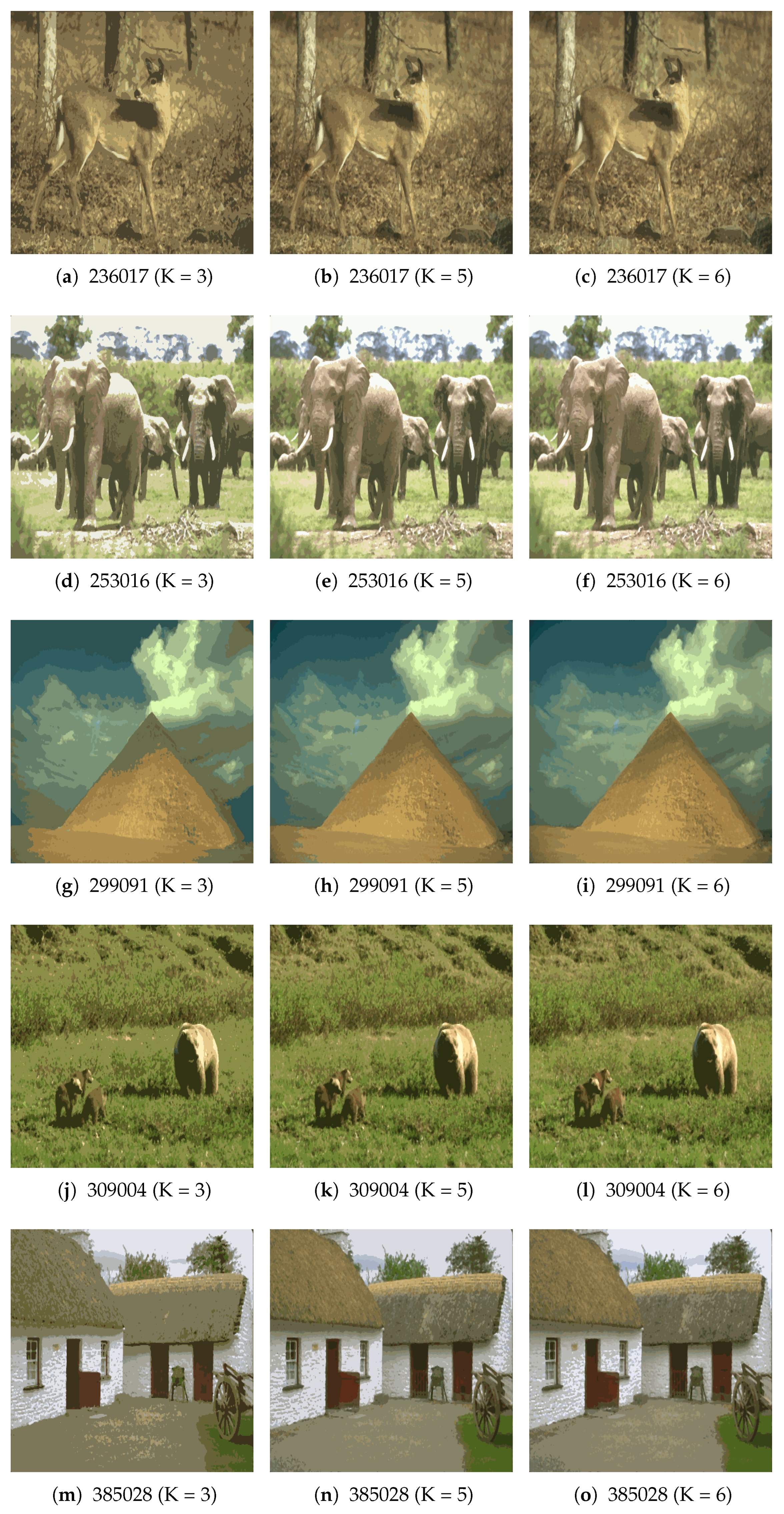
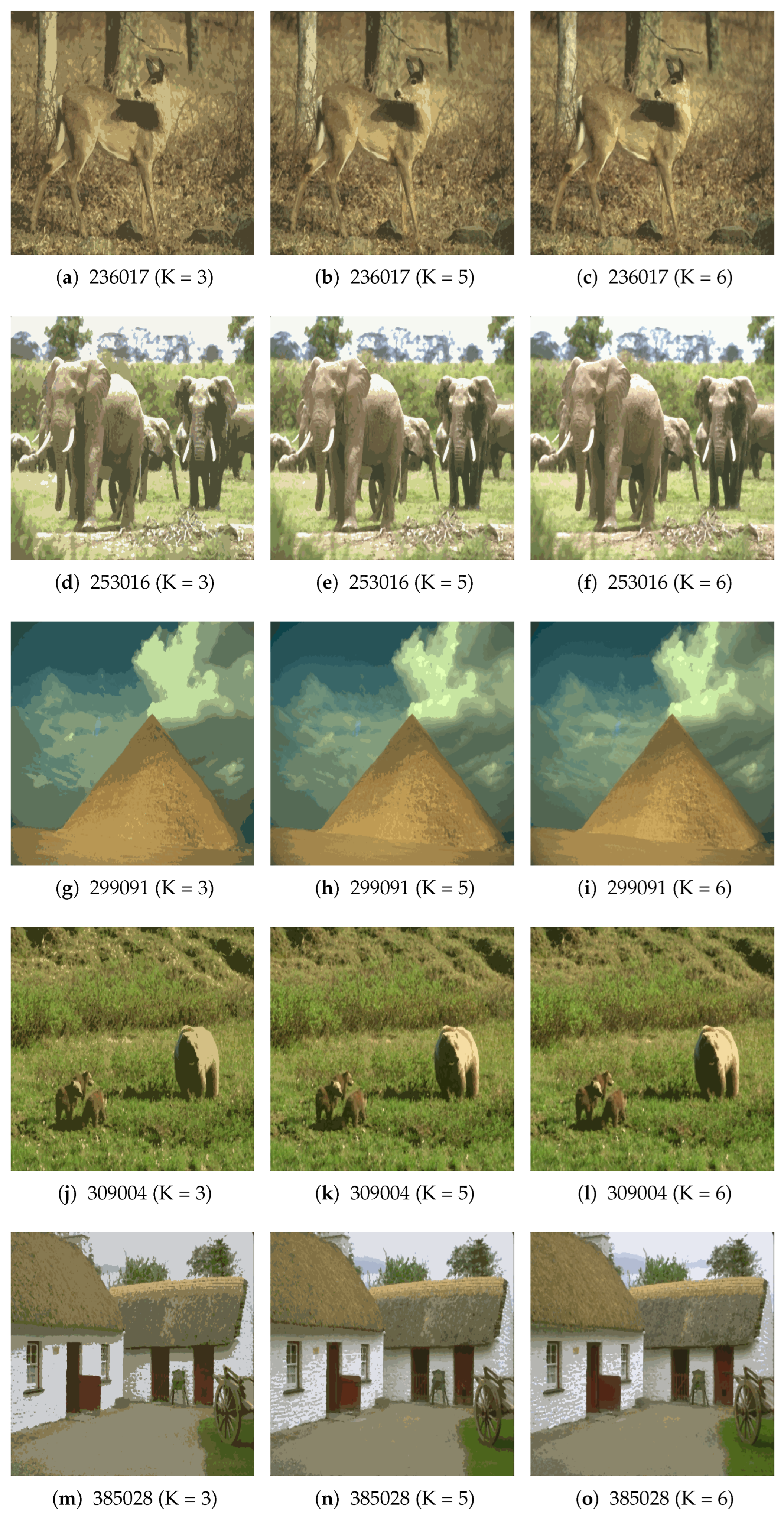
We select five representative images, namely “236017”, “253016”, “299091”, “309004”, and “385028”, to demonstrate the visual performance of MRSA. Figure 10 and Figure 11 display the results of segmented images using Kapur and Otsu.

“236017” depicts a natural scene with a prominent central object against a textured background. At K = 3, MRSA successfully separates the main foreground object from the background. The boundaries between regions are smooth and follow the natural contours of the objects. At K = 5, the background is further partitioned into sub-regions that distinguish different texture areas, while the foreground object remains a coherent whole. At K = 6, the algorithm achieves the finest granularity, and it acquires subtle variations within the background textures without introducing over-segmentation artifacts. “253016” contains multiple textures and color variations. At K = 3, MRSA produces a coarse but semantically meaningful partition that separates the major texture regions. As K increases to 5, the algorithm successfully distinguishes finer texture patterns while preserving the integrity of homogeneous areas. At K = 6, MRSA captures the most detailed texture variations, with region boundaries closely following the natural edges of the textured surfaces. “299091” includes multiple objects with overlapping color distributions. At K = 3, MRSA produces a coarse segmentation that identifies the major structural components of the scene. At K = 5, the algorithm achieves a more detailed partition, and it successfully separates objects with similar color characteristics that are often merged by other methods. At K = 6, MRSA captures fine structural details while obtaining a coherent overall segmentation structure. “309004” features smooth color gradients, but the challenge lies in preventing abrupt artifacts by maintaining smooth transitions. MRSA demonstrates a superior ability to handle such gradients: at K = 3, the algorithm produces a smooth and natural-looking segmentation that respects the global color distribution. At K = 5, additional thresholds are allocated to regions with more pronounced color variations, and it achieves finer distinctions without creating artificial boundaries in homogeneous gradient areas. At K = 6, MRSA further refines the segmentation, so it acquires subtle color nuances while preserving the visual continuity of the scene. “385028” contains fine structural details that require precise threshold placement to preserve object boundaries. At K = 3, MRSA successfully identifies the major structural components of the scene. At K = 5 and 6, the algorithm progressively captures finer details, with segmentation boundaries that align closely with the natural edges in the image.

For all five test images, MRSA demonstrates consistent visual quality under the three threshold levels based on the Kapur and Otsu criteria. The most notable observation is that the segmentation masks preserve good region consistency, while progressively capturing finer details as K increases from 3 to 6. In images “299091” and “309004”, MRSA provides a natural visual appearance and preserves perceptual consistency across varying threshold levels.

4.6. Discussion on the Entire BSD500 Dataset

To further evaluate the scalability of the proposed MRSA, we extend our experiments to the entire BSD500 dataset and K = 10 thresholds, an extremely high-dimensional search space.

4.6.1. Discussion on Kapur Entropy

Table 19. The experimental results using Kapur.

Metric	Thresholds	IBES	GGPC	MALA	RSA	MRSA
Fitness	3	13.3324	14.6299	15.1809	15.0776	15.0331
	5	18.9056	19.2476	20.3346	18.4421	20.2525
	6	21.4943	21.2780	16.4239	20.2094	22.5830
	10	30.5226	28.2710	6.2216	10.5977	30.5680
PSNR	3	15.7201	14.2942	16.9622	14.9119	17.5203
	5	19.7418	14.3207	20.0155	13.5247	20.9338
	6	21.2741	14.6364	17.7493	13.3745	22.1872
	10	25.6763	14.6639	13.6042	13.8039	25.1078
SSIM	3	0.4690	0.4025	0.4690	0.4167	0.5237
	5	0.6269	0.4442	0.5875	0.3976	0.6729
	6	0.6833	0.4719	0.5256	0.4001	0.7215
	10	0.8097	0.5038	0.4480	0.4635	0.8140
FSIM	3	0.6914	0.6669	0.7163	0.6766	0.7266
	5	0.7689	0.6707	0.7755	0.6488	0.7996
	6	0.7974	0.6748	0.7314	0.6481	0.8247
	10	0.8761	0.6759	0.6557	0.6579	0.8778
Runtime	3	2.9958	3.2081	3.1178	3.1628	8.8111
	5	3.7341	4.3938	3.7931	4.3219	8.3725
	6	4.4962	5.5699	4.7027	5.5397	8.5497
	10	10.4933	13.4314	12.9516	12.956	9.4736
RC	3	0.3931	0.3491	0.3663	0.3778	0.3938
	5	0.3334	0.3645	0.2972	0.3099	0.3590
	6	0.3131	0.3751	0.2840	0.3046	0.3575
	10	0.2381	0.3522	0.2116	0.3548	0.3480

displays the experimental results obtained using Kapur under four threshold values. As the threshold increases from 3 to 10, the objective values generally increase. Higher thresholds offer more flexibility in image segmentation. Among all the comparison methods, MRSA achieves the highest objective values at threshold numbers of 6 and 10, which are higher than those of IBES, GGPC, MALA, and RSA. At the threshold of 5, MRSA obtains 20.2525, which is only slightly lower than MALA (20.3346). When the threshold number is 3, MALA achieves the highest objective value (15.1809), whereas MRSA remains competitive with a value of 15.0331.

It can be observed that MRSA achieves the highest PSNR values at thresholds of three, five, and six. Compared with the second-best algorithm, MRSA provides noticeable improvements, especially when the threshold increases to five and six. At threshold 10, IBES (25.6763) slightly outperforms MRSA (25.1078).

MRSA achieves the highest SSIM values under all threshold numbers, with values of 0.5237, 0.6729, 0.7215, and 0.8140, respectively. The improvement is particularly obvious for threshold numbers of five and six, where MRSA significantly outperforms RSA and GGPC. Even when compared to strong competitors such as IBES and MALA, MRSA consistently exhibits the highest structural similarity.

MRSA obtains the highest FSIM values for four threshold levels. Compared to IBES, GGPC, MALA, and RSA, MRSA provides the most accurate feature preservation. The performance gain becomes more pronounced as the threshold increases, indicating that the proposed improvements remain effective for more challenging segmentation tasks.

MRSA requires more computational time when the thresholds are three, five, and six. The proposed algorithm introduces several mechanisms, which inevitably increase computational complexity. However, when the threshold number increases to 10, MRSA becomes the fastest algorithm, requiring only 9.4736 s, whereas the other algorithms require approximately between 10.49 and 13.43 s. The proposed algorithm converges more efficiently under high-dimensional search spaces and possesses better scalability for complex optimization problems.

For the threshold number three, MRSA achieves the best RC (0.3938). At threshold levels five and six, GGPC realizes the greatest values (0.3645 and 0.3751), while MRSA ranks second with values of 0.3590 and 0.3575, respectively. When the threshold increases to 10, RSA (0.3548) slightly outperforms MRSA (0.3480), whereas MRSA still remains among the top-performing methods.

The experimental findings show that the proposed MRSA achieves superior overall segmentation performance on the entire BSD500 dataset according to the Kapur entropy criterion.

4.6.2. Discussion on Otsu Criterion

Table 20. The experimental results using Otsu.

Metric	Thresholds	IBES	GGPC	MALA	RSA	MRSA
Fitness	3	2075.5747	2090.2526	2174.0292	2129.8012	2153.0586
	5	2226.5953	2179.7498	2161.6703	1910.5350	2228.7771
	6	2249.4315	2208.6741	1318.1653	1398.8620	2253.9338
	10	2285.4170	2260.2475	985.8520	1065.7043	2295.7986
PSNR	3	16.6772	14.7091	18.6209	15.4693	18.5743
	5	20.6479	14.5494	20.5143	13.4786	21.3804
	6	22.0935	14.7207	17.2060	13.2827	22.4853
	10	26.5922	14.4439	13.6230	13.7812	25.6393
SSIM	3	0.5038	0.4382	0.5640	0.4540	0.5877
	5	0.6629	0.4697	0.6302	0.4021	0.7120
	6	0.7100	0.4906	0.5283	0.4085	0.7481
	10	0.8386	0.4998	0.4482	0.4515	0.8482
FSIM	3	0.7087	0.6751	0.7492	0.6848	0.7482
	5	0.7903	0.6712	0.7905	0.6496	0.8092
	6	0.8193	0.6746	0.7241	0.6466	0.8326
	10	0.8945	0.6705	0.6539	0.6599	0.8875
Runtime	3	2.7587	2.8987	2.7627	2.7424	8.2251
	5	3.8214	4.4375	3.9631	4.3187	8.4271
	6	4.4530	5.4659	5.1131	5.5375	8.5767
	10	10.3582	12.7637	12.8671	12.8400	9.5098
RC	3	0.3931	0.3491	0.3663	0.3778	0.3938
	5	0.3334	0.3645	0.2972	0.3099	0.3590
	6	0.3131	0.3751	0.2840	0.3046	0.3575
	10	0.2381	0.3522	0.2116	0.3548	0.3480

presents the experimental results obtained using Otsu under different threshold values. MRSA achieves the highest objective function values at threshold levels 5, 6, and 10. It outperforms IBES, GGPC, MALA, and RSA. At threshold 10, MRSA improves the objective function value by approximately 10% compared to the second-best algorithm IBES. It maintains strong global optimization capability even as the search space becomes significantly larger. Only at threshold three, MALA obtains the highest objective function value (2174.0292), but it still clearly outperforms IBES, GGPC, and RSA.

At threshold levels of five and six, MRSA achieves the best PSNR values and outperforms the other comparison algorithms. When the threshold increases to 10, IBES acquires the highest PSNR value (26.5922), while MRSA ranks second with 25.6393. It’s noteworthy that at the three threshold level, the PSNR value of MRSA (18.5743) closely matches that of the superior algorithm MALA (18.6209).

MRSA obtains the highest SSIM scores across all threshold levels. Compared to IBES, MRSA further improves the SSIM to 0.8482 at a threshold level of 10. It exhibits superior ability to preserve the structural information of the original image. As the threshold increases, the SSIM values of all algorithms generally improve; however, MRSA maintains the best performance across all threshold settings.

MRSA achieves the greatest FSIM results at thresholds five and six. At threshold three, the FSIM of MRSA (0.7482) is almost identical to that of the best-performing algorithm MALA (0.7492). When the threshold increases to 10, IBES slightly outperforms MRSA; however, the performance gap between the two algorithms remains very small.

The running time of MRSA is longer than that of IBES, GGPC, MALA, and RSA at threshold levels three, five, and six. When the threshold reaches 10, MRSA requires only 9.5098 s, which is less than IBES, GGPC, MALA, and RSA. It becomes the fastest algorithm under this more challenging optimization scenario.

At a threshold level of three, MRSA achieves the highest RC. At thresholds of five and six, GGPC ranks first, while MRSA attains the second-best results. When the threshold increases to 10, RSA obtains the highest RC value (0.3548), followed by MRSA with 0.3480. Although MRSA does not achieve the best RC value at all thresholds, it consistently ranks among the top two algorithms. The performance of other algorithms shows significant fluctuations.

As the threshold level increases, the optimization landscape becomes considerably more complex. The elite-guided learning and repair mechanisms enable MRSA to identify promising regions more efficiently, thereby reducing unnecessary search efforts. Consequently, although MRSA introduces additional computational operations per iteration, its faster convergence partially compensates for this overhead at higher threshold levels, resulting in shorter overall execution times than the comparison algorithms for K = 10.

These experimental results demonstrate that the proposed MRSA can achieve high segmentation accuracy while effectively preserving image visual quality and region consistency. In particular, under high-threshold settings, MRSA exhibits superior optimization capability and overall performance compared to the comparison algorithms.

5. Conclusions

To improve the performance of multi-threshold color image segmentation, a novel framework is suggested. It integrates symmetric RGB channel cooperation, solution repair, and modified RSA. Its performance is evaluated by comparing it with IBES, MALA, GGPC, and RSA using 20 benchmark images. The experimental results based on the Kapur criterion show that MRSA outperforms the comparison algorithms on 28, 17, 57, 52, and 59 image-threshold combinations in terms of the objective function value, RC, PSNR, SSIM, and FSIM, respectively. Under the Otsu method, MRSA achieves superior performance on 15, 26, 49, 55, and 42 cases for these five metrics, respectively. Ablation experiments are conducted to further investigate the impact of the proposed improvement strategies on MRSA. The results show that these components are instrumental in improving the algorithm’s performance in multi-level thresholding image segmentation tasks. To further validate the segmentation performance of the proposed algorithm on color images, we conduct experiments on the full BSD500 dataset.

Although MRSA achieves superior segmentation performance in terms of objective function values and image quality metrics, its computational cost is generally higher than that of several comparison methods. The reason is primarily due to the introduction of the additional RGB channel cooperation mechanism, the threshold repair strategy, and the elite-guided learning process in MRSA. Therefore, the proposed method may not be suitable for strict real-time applications or ultra-high-resolution image segmentation tasks where computational efficiency is the primary concern. Future work will focus on reducing the computational complexity of MRSA through parallel implementation, lightweight cooperation mechanisms, and GPU-based acceleration.

References

1. Wang, Y.; Bao, Z.; Zhu, Q.; Lei, X. Multi-Threshold Image Segmentation Based on Reinforcement Learning–Thermal Conduction–Sine Cosine Algorithm (RLTCSCA): Symmetry-Driven Optimization for Image Processing. Symmetry 2025, 17, 2120. [Google Scholar] [CrossRef]
2. Hrizi, D.; Tbarki, K.; Elasmi, S. Optimized Lung Nodule Classification Using CLAHE-Enhanced CT Imaging and Swin Transformer-Based Deep Feature Extraction. J. Imaging 2025, 11, 346. [Google Scholar] [CrossRef] [PubMed]
3. Rao, B.; Jiang, S.; Lu, C.; Gu, Q.; Cui, Z.; Jiang, G.; Li, G. Self-supervised segmentation of large-scale blasted heap block from UAV image: Addressing block adhesion and imbalanced samples. Complex Intell. Syst. 2026, 12, 211. [Google Scholar] [CrossRef]
4. Pan, J.S.; Wei, Y.N.; Chi, L.D.; Chu, S.C.; Wang, R.Y.; Watada, J. An APO Algorithm Based on Taguchi Methods and Its Application in Multi-Level Image Segmentation. Comput. Mater. Contin. 2026, 87, 1. [Google Scholar] [CrossRef]
5. Kalpana, M.; Kumar, V.N. Enhanced Walking Palm Tree Optimization for High-Quality Multilevel Thresholding of RGB Histogram-Based Color Satellite Image Segmentation. Syst. Soft Comput. 2026, 8, 200502. [Google Scholar] [CrossRef]
6. Huang, J.; Heidari, A.A.; Liu, L.; Shao, Q.; Chen, H.; Chen, X. Rime Algorithm with Partial Reinforcement and Edge Strategies for Lupus Nephritis Image Segmentation. Appl. Soft Comput. 2026, 186, 114178. [Google Scholar] [CrossRef]
7. Şahin, M.F.; Anka, F. An adaptive hybrid metaheuristic algorithm for satellite images in remote sensing image segmentation: MF Sahin, F. Anka. Vis. Comput. 2026, 42, 134. [Google Scholar] [CrossRef]
8. Mohan, D.S.; Chandar, K.P. A Brown Bear Optimization Driven RGB–Sobel Histogram Fusion Approach for Robust Color Image Segmentation. Symmetry 2026, 18, 795. [Google Scholar] [CrossRef]
9. Zhang, X.; Wang, B.; Shao, Y.; Wang, J. A Multi-Strategy Improved Information Acquisition Algorithm for Numerical Optimization and Artistic Image Segmentation. Symmetry 2026, 18, 708. [Google Scholar] [CrossRef]
10. Brajević, I.; Ignjatović, J. Multilevel thresholding of color images using globally informed artificial bee colony algorithm. Sci. Rep. 2025, 15, 22041. [Google Scholar] [CrossRef] [PubMed]
11. Huang, S.; Ma, Y.; Wu, R.; Li, Z. A Fractional-Order Self-Learning Sparrow Search Algorithm for Multithreshold Image Segmentation. Int. J. Intell. Syst. 2026, 2026, 3010115. [Google Scholar] [CrossRef]
12. Rather, S.A.; Roy, P.P. Lévy flight and chaos-enhanced gravitational search algorithm with U-Net++ for multi-threshold brain MRI segmentation. Evol. Intell. 2026, 19, 39. [Google Scholar] [CrossRef]
13. Wang, X.; Snášel, V.; Mirjalili, S.; Pan, J.S. MAAPO: An innovative membrane algorithm based on artificial protozoa optimizer for multilevel threshold image segmentation. Artif. Intell. Rev. 2025, 58, 324. [Google Scholar] [CrossRef]
14. Abualigah, L.; Almotairi, K.H.; Elaziz, M.A. Multilevel thresholding image segmentation using meta-heuristic optimization algorithms: Comparative analysis, open challenges and new trends. Appl. Intell. 2023, 53, 11654–11704. [Google Scholar]
15. Abualigah, L.; Abd Elaziz, M.; Sumari, P.; Geem, Z.W.; Gandomi, A.H. Reptile Search Algorithm (RSA): A nature-inspired meta-heuristic optimizer. Expert Syst. Appl. 2022, 191, 116158. [Google Scholar] [CrossRef]
16. Abualigah, L.; Al-Okbi, N.K.; Alomari, S.A.; Almomani, M.H.; Moneam, S.; Yousif, M.A.; Snasel, V.; Saleem, K.; Smerat, A.; Ezugwu, A.E. Optimized image segmentation using an improved reptile search algorithm with Gbest operator for multi-level thresholding. Sci. Rep. 2025, 15, 12713. [Google Scholar] [CrossRef] [PubMed]
17. Zhao, X.; Zhu, L.; Wu, B. An improved mayfly algorithm based on Kapur entropy for multilevel thresholding color image segmentation. J. Intell. Fuzzy Syst. 2023, 44, 365–380. [Google Scholar] [CrossRef]
18. Jia, H.; Su, Y.; Rao, H.; Liang, M.; Abualigah, L.; Liu, C.; Chen, X. Improved artificial rabbits algorithm for global optimization and multi-level thresholding color image segmentation. Artif. Intell. Rev. 2024, 58, 55. [Google Scholar] [CrossRef]
19. Song, H.; Wang, J.; Bei, J.; Wang, M. Modified snake optimizer based multi-level thresholding for color image segmentation of agricultural diseases. Expert Syst. Appl. 2024, 255, 124624. [Google Scholar] [CrossRef]
20. Chaoxi, L.; Lifang, H.; Songwei, H.; Bin, H.; Changzhou, Y.; Lingpan, D. An improved bald eagle algorithm based on Tent map and Levy flight for color satellite image segmentation. Signal Image Video Process. 2023, 17, 2005–2013. [Google Scholar] [CrossRef]
21. Seyyedabbasi, A. A hybrid multi-strategy optimization metaheuristic algorithm for multi-level thresholding color image segmentation. Appl. Sci. 2025, 15, 7255. [Google Scholar] [CrossRef]
22. Wu, B.; Zhu, L.; Li, X. Giza pyramids construction algorithm with gradient contour approach for multilevel thresholding color image segmentation. Appl. Intell. 2023, 53, 21248–21267. [Google Scholar] [CrossRef]
23. Rao, H.; Jia, H.; Zhang, X.; Abualigah, L. Hybrid adaptive crayfish optimization with differential evolution for color multi-threshold image segmentation. Biomimetics 2025, 10, 218. [Google Scholar] [CrossRef] [PubMed]
24. Tao, L.; Li, L.; Lu, F. Multi-Mechanism Artificial Lemming Algorithm for Global Optimization and Color Multi-Threshold Image Segmentation. Biomimetics 2026, 11, 161. [Google Scholar] [CrossRef] [PubMed]
25. Jia, H.; Wen, C.; Rao, H.; Abualigah, L.; Abdel-Salam, M. Multi-strategy remora optimization algorithm for color multi-threshold image segmentation. PLoS ONE 2026, 21, e0342261. [Google Scholar] [CrossRef] [PubMed]
26. Zhang, X.; Bao, Z.; Li, X.; Wang, J. Multi-Threshold Art Symmetry Image Segmentation and Numerical Optimization Based on the Modified Golden Jackal Optimization. Symmetry 2025, 17, 2130. [Google Scholar] [CrossRef]
27. Liu, Y.; Wang, C.; Lu, M.; Yang, J.; Gui, J.; Zhang, S. From simple to complex scenes: Learning robust feature representations for accurate human parsing. IEEE Trans. Pattern Anal. Mach. Intell. 2024, 46, 5449–5462. [Google Scholar] [CrossRef] [PubMed]
28. Wang, S.; Wang, C.; Shi, C.; Liu, Y.; Lu, M. Mask-guided mamba fusion for drone-based visible-infrared vehicle detection. IEEE Trans. Geosci. Remote Sens. 2024, 62, 5005712. [Google Scholar] [CrossRef]
29. Martin, D.; Fowlkes, C.; Tal, D.; Malik, J. A database of human segmented natural images and its application to evaluating segmentation algorithms and measuring ecological statistics. In Proceedings Eighth IEEE International Conference on Computer Vision. ICCV 2001; IEEE: New York, NY, USA, 2001; Volume 2, pp. 416–423. [Google Scholar]
Figure 1. The segmentation process of color images.
Symmetry 18 01330 g001
Figure 2. The RC values using Kapur.
Symmetry 18 01330 g002
Figure 3. The PSNR values using Kapur.
Symmetry 18 01330 g003
Figure 4. The SSIM values using Kapur.
Symmetry 18 01330 g004
Figure 5. The FSIM values using Kapur.
Symmetry 18 01330 g005
Figure 6. The RC values using Otsu.
Symmetry 18 01330 g006
Figure 7. The PSNR values using Otsu.
Symmetry 18 01330 g007
Figure 8. The SSIM values using Otsu.
Symmetry 18 01330 g008
Figure 9. The FSIM values using Otsu.
Symmetry 18 01330 g009
Figure 10. The thresholded images of MRSA based on Kapur.
Symmetry 18 01330 g010
Figure 11. The thresholded images of MRSA based on Otsu.
Symmetry 18 01330 g011