Symmetry-Preserving Physics-Informed Neural Network Framework for Relativistic Charged-Particle Dynamics in 3+1 Dimensions

Abstract

Standard pushers for the relativistic equations of motion of a charged particle in an electromagnetic field—Boris, Vay, Higuera–Cary—do not, in general, preserve the full symplectic structure of the underlying Hamiltonian system, while high-order non-symplectic schemes such as Runge–Kutta accumulate secular error over long times. We propose a two-stage, symmetry-preserving framework (SP-PINN) for the 3+1-dimensional relativistic dynamics of a charged particle in a prescribed field, including a focused Gaussian laser pulse, that pairs a physics-informed neural network with an explicit symplectic integrator: the network learns a surrogate relativistic Hamiltonian, while the integrator—which is not itself learned—advances it. In Stage 1, an unsupervised physics-informed neural network learns the surrogate from the covariant equations of motion using a Lorentz-invariant loss that enforces the mass-shell constraint $\mathcal{H}=m{c}^2\gamma$; in Stage 2, the surrogate is advanced with an explicit symplectic map built on Tao’s extended phase space, valid for the non-separable relativistic Hamiltonian. To isolate the geometric integrator from neural-network approximation error, every benchmark figure advances the analytic relativistic Hamiltonian through Stage 2, the learned Stage-1 surrogate being assessed separately. We benchmark against the Boris pusher and Runge–Kutta on three core test problems (adding the Higuera–Cary pusher in the symplecticity diagnostic), supplemented by plane-wave, ensemble, and pulse-family studies, and we measure the first Poincaré–Cartan loop invariant directly as a quantitative diagnostic of symplecticity. The magnetic-field test illustrates the contrast between bounded and secular error growth: Runge–Kutta drifts secularly, the Boris pusher conserves the invariants to machine precision as a volume-preserving gyro-integrator, and the symplectic map keeps the error bounded for all time; on a non-integrable magnetic trap, where no exact volume-preserving rotation exists, the symplectic map alone keeps the energy error bounded. The learned surrogate is the current accuracy bottleneck—not yet competitive with the conventional pushers for the static cases—but for the demanding laser case, a vector-potential light-cone reformulation reduces this surrogate error to $(3.0\pm 0.1)\times {10}^{-4}$ (three seeds) and yields learned trajectories that remain phase-coherent over essentially the whole interaction. The framework targets laser–plasma acceleration, synchrotron-radiation modeling, and particle tracking.

1. Introduction

Relativistic charged-particle dynamics in intense electromagnetic fields is a central problem in plasma physics, laser–matter interaction, and high-energy accelerator science. The rapid development of petawatt-class laser facilities has made it experimentally feasible to accelerate electrons to GeV-scale energies over centimeter-scale distances via laser wakefield acceleration (LWFA), generating ultra-short, high-brightness particle beams unattainable with conventional radio-frequency accelerators [1,2]. In these extreme regimes—where the normalized laser vector potential satisfies $a_0=eA/m{c}^2\gg 1$—the particle dynamics become intrinsically relativistic, and even small numerical errors in the equations of motion accumulate rapidly, leading to qualitatively incorrect physical predictions. Accurate long-term integration of the relativistic Lorentz-force equation is therefore essential for the predictive simulation of these systems.

The standard workhorse of particle-in-cell (PIC) codes for solving the relativistic equations of motion is the Boris pusher [3], supplemented by the later improvements of Vay [4] and Higuera and Cary [5]. The Boris algorithm is volume preserving and second-order accurate in time, but it is not symplectic in the strict sense: it does not exactly preserve the symplectic two-form $\omega =\mathrm{d}\mathbf{P}\wedge \mathrm{d}\mathbf{q}$ of the underlying Hamiltonian system [6,7]. As a consequence, long-time integrations with the Boris pusher can accumulate a non-physical secular drift (an error growing without bound, typically linearly in integration time, as opposed to a bounded oscillation) of geometric phase-space invariants, even while the gyro-orbit radius itself is preserved with remarkable accuracy [8,9]. The Vay integrator correctly preserves the $\mathbf{E}\times \mathbf{B}$ drift velocity but likewise does not satisfy strict symplecticity, and higher-order Runge–Kutta (RK4) methods, while accurate over short intervals, fail to conserve the geometric structure of phase space for nonlinear Hamiltonian systems over long integration times [10].

To overcome these limitations, structure-preserving numerical methods—symplectic integrators—have been developed, which preserve the symplectic form exactly and hence, through backward error analysis, conserve the corresponding integrals of motion up to exponentially small corrections over arbitrarily long times [10,11]. For non-relativistic charged particles, explicit high-order symplectic integrators of the Yoshida and Forest–Ruth type are well established [11,12]. For relativistic dynamics the situation is more complex, since the relativistic Hamiltonian $\mathcal{H}=c\sqrt{{(\mathbf{P}-e\mathbf{A}/c)}^2+m^2{c}^2}+e\phi$ is non-separable in general electromagnetic fields, precluding a straightforward splitting. Explicit high-order symplectic integrators for charged particles in general fields were constructed by Tao through an extended phase-space formulation [13]; volume-preserving second-order methods for relativistic trajectories were derived by Higuera and Cary [5] (structure-preserving but, like Boris, not symplectic, as we confirm in Section 5.7); volume-preserving algorithms for charged-particle dynamics were developed by He et al. [14]; and a comprehensive comparison of relativistic particle pushers was performed by Ripperda et al. [15]; recent additions to this structure-preserving relativistic line include the error-controlled scheme of Zhang et al. [16] and the well-posed pusher of Zhou and Zhang [17]. Nevertheless, a framework that simultaneously guarantees (i) a Lorentz-invariant Hamiltonian structure, (ii) explicit high-order symplecticity, and (iii) applicability to prescribed, time-dependent fields such as Gaussian laser pulses remains an open problem.

In parallel, the paradigm of physics-informed neural networks (PINNs), introduced by Raissi, Perdikaris, and Karniadakis [18] (see [19] for a comprehensive review), embeds physical laws directly in neural-network training through residual loss functions. In Hamiltonian mechanics, Hamiltonian Neural Networks [20] and symplectic networks (SympNets) [21] learn the system Hamiltonian and enforce energy conservation by construction; subsequent work has extended these ideas to generalized and constrained Hamiltonian systems [22,23,24], and recent work develops symplectic, Lie–Poisson, and pseudo-symplectic neural integrators [25,26,27,28]. In particular, unsupervised Hamiltonian neural networks recover the surrogate ${\mathcal{H}}_{\theta }(\mathbf{q},\mathbf{p})$ from the equations of motion alone, using no integrated trajectories as supervised targets [29], after which it can be advanced with a structure-preserving integrator. To date, however, these approaches have been developed for classical low-dimensional systems and have not been combined with an explicit symplectic map for relativistic dynamics governed by Lorentz-covariant Hamiltonian structure in 3+1 dimensions, which is the gap addressed here.

The present work builds directly on the Lorentz-invariant Lagrangian–Hamiltonian framework developed by the authors. In [30], we derived the Lagrangian and Hamiltonian formalisms for relativistic mechanics in terms of Lorentz-invariant evolution parameters, establishing the covariant canonical structure. In [31], we introduced a coupled-parameter hyperbolic parametrization of the Lorentz coordinates in terms of rapidity $\theta$ and Lorentz factor $\gamma$, demonstrating the mutual invertibility $\gamma \left(\theta \right)$ and $\theta \left(\gamma \right)$ as analytic integrals of motion. More recently [32], integrals of motion for a relativistic particle in 1+1 dimensions were obtained in terms of generalized inverse energy–momentum functions, and the dynamics of a relativistic particle in the field of a Gaussian laser pulse were analyzed in [33]. Invariant descriptions of the classical relativistic particle motion in 3+1 dimensions were subsequently derived in [34], and the dynamics of relativistic particles in an ion-cyclotron trap driven by an external ultrashort laser pulse were studied in [35]. The SP-PINN framework proposed here integrates these results into a unified, symmetry-preserving numerical integrator for the 3+1-dimensional problem.

The main contributions of this work are as follows:

• We formulate the SP-PINN integrator for a relativistic charged particle in a 3+1-dimensional prescribed electromagnetic field, including a Gaussian laser pulse, within the Lorentz-invariant Hamiltonian framework of [30,31].
• An unsupervised PINN learns the relativistic Hamiltonian surrogate ${\mathcal{H}}_{\theta }$ from a loss incorporating the covariant equations of motion, the mass-shell constraint $\mathcal{H}=m{c}^2\gamma$, and boundary conditions from the analytic integrals of motion.
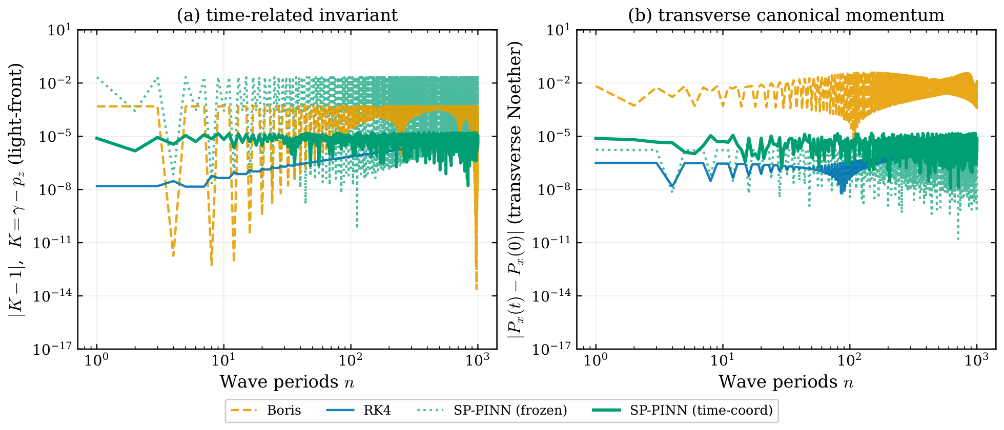
• The learned Hamiltonian is advanced with an explicit symplectic map [11,13], preserving the Poincaré–Cartan invariant and the Lorentz-group orbit structure of phase space; promoting time to a canonical coordinate restores exact symplecticity for time-dependent fields, improving conservation of the light-front invariant by about three orders of magnitude (Appendix A.1).
• Performance is benchmarked against RK4 and the Boris pusher in terms of geometric-invariant conservation, symplecticity diagnostics, and trajectory accuracy, with all simulation code released openly [36].

We are explicit about what is and is not new here. The Stage-2 geometric integrator is Tao’s explicit extended-phase-space symplectic map [13], used here unchanged, and the two-stage idea of learning a Hamiltonian surrogate and then integrating it symplectically follows the structure-preserving neural-integrator line [20,21,29]. Most directly, the unsupervised-PINN-Hamiltonian-plus-fourth-order-Yoshida combination has very recently been proposed independently by Liang et al. (SPINI [37]) for non-relativistic, separable systems (a nonlinear pendulum), and symplectic neural networks have been applied to charged-particle dynamics in electromagnetic fields by Drimalas et al. [38], who learn the symplectic map directly and report sub-gyroperiod accuracy against the Boris pusher. Closest to the present work on the non-separability axis, Cheng et al. [26] learn non-separable Hamiltonian systems with a pseudo-symplectic neural network—a construction whose discrete flow deviates from a symplectomorphism at a prescribed high order in the step size rather than preserving the symplectic form exactly, and which is developed for classical, non-relativistic systems. Relative to these, the present work is specifically relativistic and covariant: the learned object is a Lorentz-covariant Hamiltonian for the non-separable relativistic problem—where the standard separable Yoshida splitting does not apply and Tao’s extended phase space is required, and where the Stage-2 map is (for an autonomous surrogate) exactly symplectic by construction rather than symplectic to a finite order—demonstrated in 3+1 dimensions including a focused laser pulse. A parallel line embeds conservation structure into the network itself: conservative PINNs enforce local conservation laws across subdomain interfaces [39], and—most closely related to the geometric side of our approach—multi-symplectic PINNs have very recently been developed by Yan, Hu and co-workers for nonlinear infinite-dimensional (field-theoretic) Hamiltonian systems and generalized to non-conservative and quantum-tunneling settings [40,41]. Those works preserve the multi-symplectic structure of Hamiltonian partial differential equations discretized on a space–time grid; the present method instead targets a finite-dimensional, non-separable relativistic single-particle Hamiltonian, learning a Lorentz-covariant ${\mathcal{H}}_{\theta }$ and advancing it with Tao’s extended-phase-space canonical-symplectic map. The two therefore occupy complementary corners of structure-preserving PINN design—infinite- versus finite-dimensional, multi-symplectic PDE versus canonical-symplectic ODE—and the covariant mass-shell constraint used here has no direct analogue in the multi-symplectic-PDE setting.

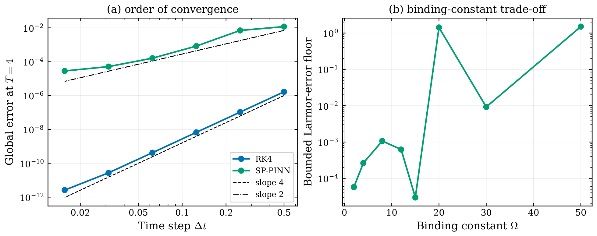
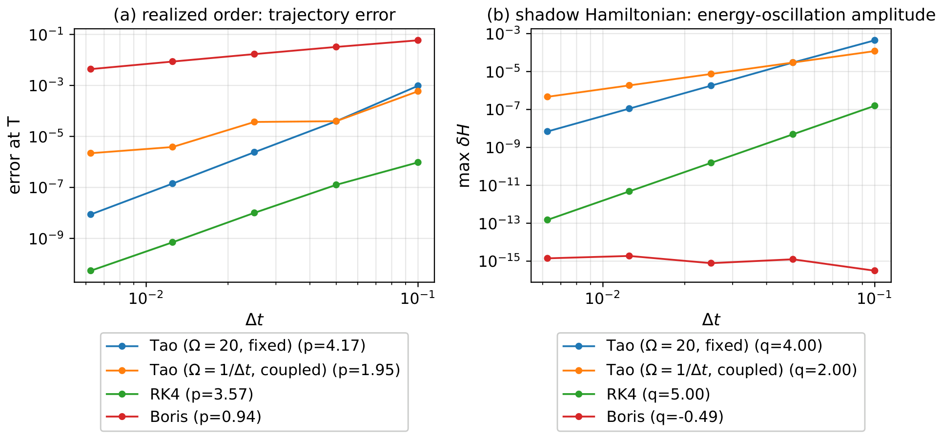
The new elements of the present work are: (i) the formulation of the surrogate-learning loss for a relativistic, Lorentz-covariant Hamiltonian with an explicit mass-shell constraint $\mathcal{H}=m{c}^2\gamma$, which ties the learned object to the coadjoint-orbit (mass-hyperboloid) geometry of the Lorentz group; and (ii) the demonstration of the symplectic pipeline on 3+1-dimensional charged-particle dynamics in prescribed fields (including a focused Gaussian laser pulse), both with the analytic Hamiltonian—which isolates the geometric integrator—and, for the laser, with a learned vector-potential surrogate driven end-to-end through the complete two-stage map. We do not claim a new symplectic integrator; we claim a symmetry-aware way of supplying one with a relativistic Hamiltonian, and an assessment of where this currently helps and where it does not. In particular, every comparison figure uses the analytic Hamiltonian in Stage 2; the learned Stage-1 surrogate is assessed separately (Section 6), where a vector-potential light-cone formulation reproduces the demanding time-dependent 3+1D laser trajectory phase-coherently over essentially the whole interaction, leaving only the final closing of the surrogate-accuracy gap (${\epsilon }_{\theta }\lesssim {10}^{-4}$) to future work. More broadly, we delimit the scope deliberately: the contribution is the single-particle, structure-preserving method together with its demonstration—including the near-axis learned laser pipeline and a cold-bunch ensemble proof-of-concept (Section 5.9)—whereas the two quantitative characterizations it points to, namely the law that amplifies a small surrogate-force error into trajectory error and the scaling of ${\epsilon }_{\theta }$ with the training-tube width needed to cover a realistic warm-bunch emittance, are deferred to a dedicated companion study and are not prerequisites for any result reported here. We also flag at the outset two operating regimes of the Stage-2 map. At fixed binding constant $\Omega$—the mode used in all trajectory figures of Section 5—the map integrates the extended Hamiltonian to fourth order, down to an $\Omega$-dependent bounded error floor. To drive that floor to zero, one takes the coupled limit $\Omega \propto \Delta t^{-1}$—used only in the convergence study of Appendix A.2—in which the realized order on the true trajectory is second, not fourth, because the residual binding error caps it (the mechanism—an oscillatory, zero-mean binding error—is detailed in Section 4 and Appendix A.2). Either way the benefit of the method is the absence of secular error growth, not a higher formal order.

Conceptually, the construction makes a symmetry of the training objective the source of the integrator’s structure preservation: a Lorentz-invariant loss biases the surrogate toward the covariant mass-shell geometry, which the symplectic map then preserves as a Lorentz-group orbit (Section 6)—the feature that places this work within the scope of structure- and symmetry-preserving computation.

The remainder of the paper is organized as follows. Section 2 presents the covariant Lagrangian–Hamiltonian framework and the field configuration. Section 3 discusses the symplectic structure and the Poincaré–Cartan invariant. Section 4 describes the SP-PINN architecture, loss function, and integration scheme. Section 5 presents numerical results, Section 6 discusses their implications, and Section 7 concludes.

2. Relativistic Hamiltonian Formalism in 3+1 Dimensions

2.1. Covariant Lagrangian and Hamiltonian of a Charged Particle

Throughout this section, we use Gaussian (CGS) units, in which the electromagnetic coupling enters through the combination $e\mathbf{A}/c$, the field–momentum relation reads $\mathbf{E}=-\frac{1}{c}{\partial }_t\mathbf{A}-\nabla \phi$, and the Lorentz force is $e\left(\mathbf{E}+\frac{1}{c}\dot{\mathbf{r}}\times \mathbf{B}\right)$. The classical relativistic mechanics of a charged particle in an external electromagnetic field is naturally formulated within the variational Lagrangian–Hamiltonian framework, which makes the Lorentz symmetry of the equations of motion explicit [42,43]. The action must be a Lorentz scalar, so that the equations derived from $\delta S=0$ are covariant under the Poincaré group; this requirement, up to gauge freedom, determines the form of the Lagrangian. In an inertial frame parametrized by coordinate time t, the Lagrangian of a particle of mass m and charge e in a field with four-potential $A^{\mu }=(\phi /c,\mathbf{A})$ reads [42,44]

$$\mathcal{L}(\mathbf{r},\dot{\mathbf{r}},t)=-m{c}^2\sqrt{1-{\displaystyle \frac{{\dot{\mathbf{r}}}^2}{c^2}}}+{\displaystyle \frac{e}{c}}\mathbf{A}·\dot{\mathbf{r}}-e\phi ,$$

(1)

where $\gamma ={(1-{\dot{\mathbf{r}}}^2/c^2)}^{-1/2}$. The canonical momentum conjugate to $\mathbf{r}$ is

$$\mathbf{P}={\displaystyle \frac{\partial \mathcal{L}}{\partial \dot{\mathbf{r}}}}=\gamma m\dot{\mathbf{r}}+{\displaystyle \frac{e}{c}}\mathbf{A}=\mathbf{p}+{\displaystyle \frac{e}{c}}\mathbf{A},$$

(2)

where $\mathbf{p}=\gamma m\dot{\mathbf{r}}$ is the kinetic momentum. Because $\mathbf{P}$ is gauge dependent while $\mathbf{p}$ is not, the two must be distinguished in the Hamiltonian formulation and in identifying gauge-invariant conserved quantities. The Legendre transformation yields

$$\mathcal{H}(\mathbf{r},\mathbf{P},t)=\mathbf{P}·\dot{\mathbf{r}}-\mathcal{L}=c\sqrt{{\left(\mathbf{P}-{\displaystyle \frac{e}{c}}\mathbf{A}\right)}^2+m^2{c}^2}+e\phi ,$$

(3)

the exact relativistic Hamiltonian, from which Hamilton’s canonical equations follow:

$$\dot{\mathbf{r}}={\displaystyle \frac{\partial \mathcal{H}}{\partial \mathbf{P}}}={\displaystyle \frac{c(\mathbf{P}-\frac{e}{c}\mathbf{A})}{\sqrt{{(\mathbf{P}-\frac{e}{c}\mathbf{A})}^2+m^2{c}^2}}},\dot{\mathbf{P}}=-{\displaystyle \frac{\partial \mathcal{H}}{\partial \mathbf{r}}}.$$

(4)

Upon substitution, these reproduce the relativistic Lorentz-force equation $\mathrm{d}\mathbf{p}/\mathrm{d}t=e\left(\mathbf{E}+\frac{1}{c}\dot{\mathbf{r}}\times \mathbf{B}\right)$ [44]. Along any physical trajectory $\mathcal{H}=\gamma m{c}^2+e\phi$; in the radiation gauge ($\phi =0$), this reduces to $\mathcal{H}=\gamma m{c}^2$. Following [30], the proper time $\tau$ may be employed as the evolution parameter, rendering the canonical equations manifestly covariant first-order ordinary differential equations on the extended phase space $(\mathbf{r},\mathbf{P},t,-\mathcal{H})$.

2.2. Lorentz Symmetry and Integrals of Motion

The Lorentz-invariant structure of the system admits exact first integrals that are direct manifestations of Poincaré symmetry [30,31]. The mass-shell constraint

$$p^{\mu }{p}_{\mu }={\left({\displaystyle \frac{\mathcal{E}}{c}}\right)}^2-{\left|\mathbf{p}\right|}^2=m^2{c}^2,$$

(5)

with $\mathcal{E}=\gamma m{c}^2$ and $p^{\mu }=(\mathcal{E}/c,\mathbf{p})$, expresses the conservation of the Lorentz norm of the four-momentum and is preserved exactly along every physical trajectory. Geometrically the four-momentum is confined to the mass hyperboloid$\{p^{\mu }:p^{\mu }{p}_{\mu }=m^2{c}^2\}$, an orbit of the Lorentz group acting on momentum space; “preserving Lorentz structure” here means concretely keeping the numerical state on this hyperboloid. In terms of the Lorentz factor it reads ${\gamma }^2-{\left|\mathbf{p}\right|}^2/{\left(mc\right)}^2=1$ and furnishes the fundamental constraint enforced by the SP-PINN loss. In [31], a coupled-parameter hyperbolic parametrization was introduced in which the rapidity $\theta$—the additive parameter of Lorentz boosts in the Lie algebra of $\mathrm{SO}(1,3)$—plays the central role:

$$\gamma =cosh\theta ,{\displaystyle \frac{p_{\Vert }}{mc}}=sinh\theta ,$$

(6)

so that the phase-space point $(\gamma ,p_{\Vert }/mc)$ lies on the unit hyperbola ${\gamma }^2-{(p_{\Vert }/mc)}^2=1$ (the ${\mathbf{p}}_{\perp }=0$ restriction of the mass-shell), a coadjoint orbit of the Lorentz group [31,32]. The additivity of $\theta$ under boosts makes it the natural coordinate on the mass hyperboloid. For a field invariant under transverse translations—such as a plane wave or, approximately, a broad laser beam propagating along z—the transverse canonical momenta $P_x$ and $P_y$ are exact integrals of motion by Noether’s theorem, and together with $\theta$ form a complete set of first integrals used below to define the PINN boundary conditions.

2.3. Electromagnetic Field Configuration: Gaussian Laser Pulse

As a physically motivated and numerically demanding test case we consider a focused, linearly polarized Gaussian laser pulse propagating along z, consistent with the configuration analyzed in [33,45]. In the paraxial approximation, the vector potential $\mathbf{A}=A_x\widehat{\mathbf{x}}$ takes the form

$$A_x=A_0{\displaystyle \frac{w_0}{w\left(z\right)}}exp\left[-{\displaystyle \frac{x^2+y^2}{w{\left(z\right)}^2}}-{\displaystyle \frac{{(z-ct)}^2}{c^2{\tau }_L^2}}\right]cos\left[k_0(z-ct)+\psi (x,y,z)\right],$$

(7)

with $A_0=m{c}^2{a}_0/e$ fixing the amplitude through the dimensionless normalized vector potential $a_0$ (the relativistic-intensity parameter, with $a_0\gg 1$ the strongly relativistic regime), $w_0$ the beam waist (the $1/e$ transverse field radius at focus), ${\tau }_L$ the pulse duration, and $k_0={\omega }_0/c$ the carrier wavenumber, and 

$$w\left(z\right)=w_0\sqrt{1+{(z/z_R)}^2},z_R={\displaystyle \frac{k_0{w}_0^2}{2}},\psi ={\displaystyle \frac{k_0(x^2+y^2)}{2R\left(z\right)}}-arctan{\displaystyle \frac{z}{z_R}},$$

(8)

where $z_R$ is the Rayleigh length (the characteristic diffraction length, over which the beam cross-sectional area doubles). The fields follow from $\mathbf{E}=-(1/c){\partial }_t\mathbf{A}$ and $\mathbf{B}=\nabla \times \mathbf{A}$. In the plane-wave limit ($w_0\to \infty$), the field is invariant under transverse translations, implying exact conservation of $P_x$ and $P_y$; for a finite beam, this symmetry is weakly broken by diffraction, while a discrete ${\mathbb{Z}}_2$ symmetry under $x\to -x$ is retained. In the regime $a_0\gg 1$, the dynamics become strongly relativistic—the transverse quiver Lorentz factor is of order $a_0$, while an initially stationary electron acquires a ponderomotive energy gain $\langle \gamma \rangle -1\sim a_0^2/4$ (cycle-averaged), with instantaneous peaks $\gamma \approx 12$ for $a_0=5$ (Section 5.2)—making long-time structure preservation particularly important. The parameters used in Section 5 are summarized in

Table 1. Parameters of the Gaussian laser pulse used in Test Case 2 (Section 5.2). Code units set $c=1$, $m=1$, and $k_0={\omega }_0=1$; SI equivalents are given for an 800 nm laser.

Parameter	Symbol	Value
Laser wavelength	${\lambda }_0$	800 nm
Normalized vector potential	$a_0$	5
Beam waist	$w_0$	$5{\lambda }_0\approx$ 4 μm
Pulse duration	${\tau }_L$	$30{\omega }_0^{-1}$ (≈13 fs)
Rayleigh length	$z_R$	$k_0{w}_0^2/2$
Initial electron state	$({\gamma }_0,{\mathbf{p}}_0)$	$(1,\mathbf{0})$, at rest
Integration time step	$\Delta t$	$0.05{\omega }_0^{-1}$ (≈0.02 fs)
Field finite-difference step	h	${10}^{-4}$ (dimensionless, code units)

.

3. Symplectic Structure and the Poincaré–Cartan Invariant

3.1. Symplectic Form in Relativistic Phase Space

The geometric foundation of Hamiltonian mechanics is the symplectic structure of phase space [46,47,48]. For canonical coordinates $(\mathbf{q},\mathbf{P})\in {\mathbb{R}}^{2n}$, the canonical symplectic two-form $\omega ={\sum }_i\mathrm{d}{P}_i\wedge \mathrm{d}{q}^i$ is closed and non-degenerate, and Hamilton’s equations are equivalent to ${\iota }_{X_{\mathcal{H}}}\omega =\mathrm{d}\mathcal{H}$. The flow generated by any Hamiltonian vector field is a symplectomorphism: it preserves $\omega$ exactly. The Poincaré–Cartan integral invariant is built from the canonical one-form $\Theta =P_{\mu }\mathrm{d}{q}^{\mu }$,

$$I_1={\oint }_{\mathcal{C}\left(t\right)}\Theta ={\oint }_{\mathcal{C}\left(t\right)}\left(\mathbf{P}·\mathrm{d}\mathbf{q}-\mathcal{H}\mathrm{d}t\right),$$

(9)

and is conserved exactly along the flow for any closed co-moving curve $\mathcal{C}\left(t\right)$ [46]. At fixed time, it reduces to the first Poincaré invariant $I_1={\oint }_{\mathcal{C}}\mathbf{P}·\mathrm{d}\mathbf{q}=\mathrm{const}$, which provides the central computable diagnostic of symplecticity. Liouville’s theorem—preservation of the phase-space volume ${\omega }^n/n!$—is a corollary of symplecticity, but for $n\ge 2$ is strictly weaker: a map can preserve volume without preserving $\omega$ [6,9] (for $n=1$ the two coincide, since $\omega$ is then itself the area form; and because a symplectic map preserves the loop invariant on every conjugate plane, a measured drift of $\delta I_1$ on the single $(x,P_x)$ plane is already sufficient to detect non-symplecticity in the full phase space—a necessary-condition test, even though boundedness on one plane does not by itself certify symplecticity).

3.2. Violation of Symplecticity in Conventional Solvers

Standard integrators used in plasma physics do not, in general, preserve the symplectic form. The Boris pusher is volume preserving but not symplectic [6]; Qin et al. [6] showed that it conserves phase-space volume while its energy error is bounded for integrable systems but can grow secularly for non-integrable ones. RK4 is neither symplectic nor volume preserving: its per-step deviation from a symplectomorphism is $\mathcal{O}(\Delta t^5)$, and because it admits no modified Hamiltonian (only a non-conservative modified vector field), the geometric invariants generically drift secularly (typically linearly in the number of steps) rather than remaining bounded [10]. The first Poincaré invariant is monitored numerically by evolving an ensemble of M nearby phase-space points forming a closed loop $\mathcal{C}$ and evaluating

$$I_1^{\left(k\right)}={\displaystyle \sum _{j=1}^M}{\displaystyle \frac{{\mathbf{P}}_j^{\left(k\right)}+{\mathbf{P}}_{j+1}^{\left(k\right)}}{2}}·\left({\mathbf{q}}_{j+1}^{\left(k\right)}-{\mathbf{q}}_j^{\left(k\right)}\right),{\mathcal{C}}_{M+1}\equiv {\mathcal{C}}_1,$$

(10)

at each step k [49,50]. For a truly symplectic integrator, $I_1^{\left(k\right)}=I_1^{\left(0\right)}$ up to the discretization error of the loop quadrature. The relative deviation $\delta I_1\left(t\right)=|I_1\left(t\right)-I_1\left(0\right)|/|I_1\left(0\right)|$ provides a rigorous symplecticity diagnostic; for the integrable benchmarks considered below, the bounded versus secular growth of the exact scalar invariants (the Lorentz factor and the Larmor radius) is a robust signature of the same structure-preserving-versus-non-structure-preserving distinction—necessary though, since a volume-preserving non-symplectic map such as the Boris pusher also keeps them bounded, not by itself sufficient to certify symplecticity—and is the quantity we actually report in Section 5, so the reported evidence does not depend on the loop-discretization size M.

4. SP-PINN: Proposed Method

4.1. Architecture Overview

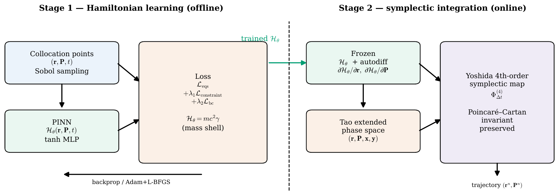
The SP-PINN integrator is a two-stage method that separates system identification from geometric integration [29]. In Stage 1, an unsupervised PINN ${\mathcal{H}}_{\theta }(\mathbf{r},\mathbf{P};t)$ is trained on collocation points in the extended phase space, with a loss combining the residual of Hamilton’s equations, the relativistic mass-shell constraint, and boundary conditions from the analytic integrals of motion [18,30,31]. In Stage 2, the trained surrogate is advanced with an explicit symplectic map. Because the symplectic map is a composition of exact canonical sub-flows, the generated discrete map is exactly symplectic with respect to ${\mathcal{H}}_{\theta }$, independently of the training error [11,13]; it is the fidelity of ${\mathcal{H}}_{\theta }$ to the true Hamiltonian—not the symplecticity of the map—that is governed by ${\epsilon }_{\theta }$, which can be reduced by improving the surrogate parametrization and collocation density. The workflow is illustrated in Figure 1; the dashed boundary separates the offline training phase from the online integration phase, the latter requiring only forward evaluations of ${\mathcal{H}}_{\theta }$ and its gradients via automatic differentiation.

4.2. Stage 1—Unsupervised PINN for Hamiltonian Learning

The surrogate ${\mathcal{H}}_{\theta }:{\mathbb{R}}^7\to \mathbb{R}$ is a fully connected feedforward network with tanh activations,

$${\mathcal{H}}_{\theta }(\mathbf{r},\mathbf{P},t)=W^{(L+1)}\sigma \left(\cdots \sigma \left(W^{\left(1\right)}[\mathbf{r};\mathbf{P};t]+{\mathbf{b}}^{\left(1\right)}\right)\cdots \right)+b^{(L+1)},$$

(11)

with $\sigma =tanh$. The smoothness of tanh guarantees that all derivatives entering the loss are well defined and computable by automatic differentiation [18]. Weights are initialized with the Xavier scheme. Concretely, the static (free-particle, magnetic-field, and non-integrable) surrogates use $L=5$ hidden layers of width 128, whereas the time-dependent vector-potential laser surrogate of Section 6 uses $L=6$ layers of width 256 (≈$3.4\times {10}^5$ trainable parameters); these and the remaining hyperparameters are specified in the released code [36]. The total objective is

$${\mathcal{L}}_{\mathrm{total}}={\mathcal{L}}_{\mathrm{eqs}}+{\lambda }_1{\mathcal{L}}_{\mathrm{constraint}}+{\lambda }_2{\mathcal{L}}_{\mathrm{bc}},$$

(12)

with the residual of Hamilton’s equations

$${\mathcal{L}}_{\mathrm{eqs}}={\displaystyle \frac{1}{N_c}}\sum _k\left[{∥{\dot{\mathbf{r}}}_k-{\displaystyle \frac{\partial {\mathcal{H}}_{\theta }}{\partial \mathbf{P}}}{|}_k∥}^2+{∥{\dot{\mathbf{P}}}_k+{\displaystyle \frac{\partial {\mathcal{H}}_{\theta }}{\partial \mathbf{r}}}{|}_k∥}^2\right],$$

(13)

the relativistic mass-shell constraint

$${\mathcal{L}}_{\mathrm{constraint}}={\displaystyle \frac{1}{N_c}}\sum _k{\left({\mathcal{H}}_{\theta }({\mathbf{r}}_k,{\mathbf{P}}_k,t_k)-m{c}^2{\gamma }_k\right)}^2,{\gamma }_k=\sqrt{1+|{\mathbf{p}}_k{|}^2/{\left(mc\right)}^2},$$

(14)

and boundary conditions enforcing the analytic integrals of motion (initial energy, rapidity, and—for the laser case—the conserved transverse momenta) at the initial collocation points [31,32],

$${\mathcal{L}}_{\mathrm{bc}}={\displaystyle \frac{1}{\left|\mathcal{B}\right|}}\sum _{k\in \mathcal{B}}\left[{\left({\mathcal{H}}_{\theta }({\mathbf{r}}_k,{\mathbf{P}}_k,t_k)-{\mathcal{E}}_0\right)}^2+{\left({\theta }_k-{\theta }_0\right)}^2+\parallel {\mathbf{P}}_{\perp ,k}-{\mathbf{P}}_{\perp }^0{\parallel }^2\right],$$

(15)

where $\mathcal{B}$ is the set of initial ($t=t_0$) collocation points and ${\mathcal{E}}_0$, ${\theta }_0$, ${\mathbf{P}}_{\perp }^0$ are the analytic initial energy, rapidity, and (laser-case) transverse momenta. The mass-shell term is the central symmetry-preserving ingredient: enforcing it throughout training biases ${\mathcal{H}}_{\theta }$ toward the hyperbolic mass-hyperboloid geometry of relativistic momentum space, the coadjoint orbit of the Lorentz group. (Here ${\mathbf{p}}_k={\mathbf{P}}_k-\frac{e}{c}\mathbf{A}({\mathbf{r}}_k,t_k)$ is the kinetic momentum, formed from the canonical network input and the known field. This $\phi =0$ form applies to the magnetic-field and laser cases trained here; for a static scalar potential, the surrogate target carries the additional $e\phi$ term, ${\mathcal{H}}_{\theta }=\gamma m{c}^2+e\phi$, and the constraint is imposed on the kinetic mass-shell.) Collocation points are drawn quasi-randomly (Sobol sequence) over the physically relevant domain; optimization proceeds with Adam followed by L-BFGS, with ${\lambda }_1=10$, ${\lambda }_2=1$ following the adaptive-weighting practice of [23,51,52]. We quantify a trained surrogate by ${\epsilon }_{\theta }$, the root-mean-square error of ${\mathcal{H}}_{\theta }$ (or, for the vector-potential variant of Section 4.4, of ${\mathbf{A}}_{\theta }$) together with its gradients, evaluated over a held-out test set.

4.3. Stage 2—Explicit Symplectic Integration

Once ${\mathcal{H}}_{\theta }$ has converged, it is treated as a fixed, differentiable Hamiltonian and advanced with an explicit symplectic integrator. Because the relativistic Hamiltonian (3) is non-separable, we employ the extended phase-space construction of Tao [13]: two copies of the system are introduced—the original $(\mathbf{r},\mathbf{P})$ and a second canonical copy$(\tilde{\mathbf{r}},\tilde{\mathbf{P}})$ (a second position–momentum pair, not the Cartesian spatial coordinates $x,y,z$ used elsewhere)—with the extended Hamiltonian

$$\overline{\mathcal{H}}={\mathcal{H}}_{\theta }(\mathbf{r},\tilde{\mathbf{P}})+{\mathcal{H}}_{\theta }(\tilde{\mathbf{r}},\mathbf{P})+{\displaystyle \frac{\Omega }{2}}\left(\parallel \mathbf{r}-\tilde{\mathbf{r}}{\parallel }^2+{\parallel \mathbf{P}-\tilde{\mathbf{P}}\parallel }^2\right).$$

(16)

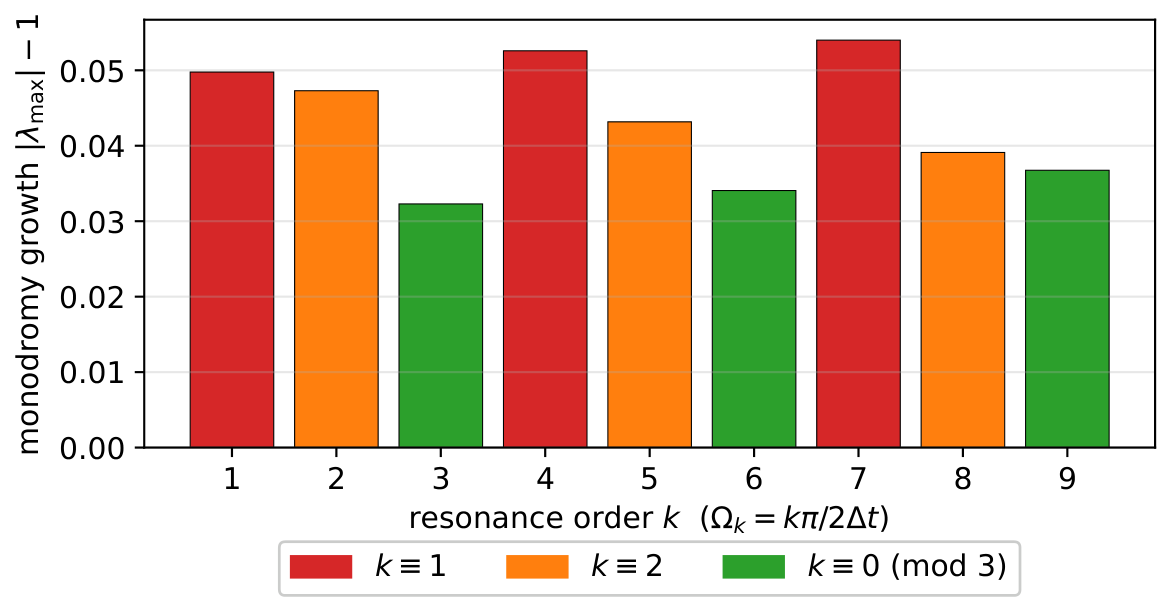
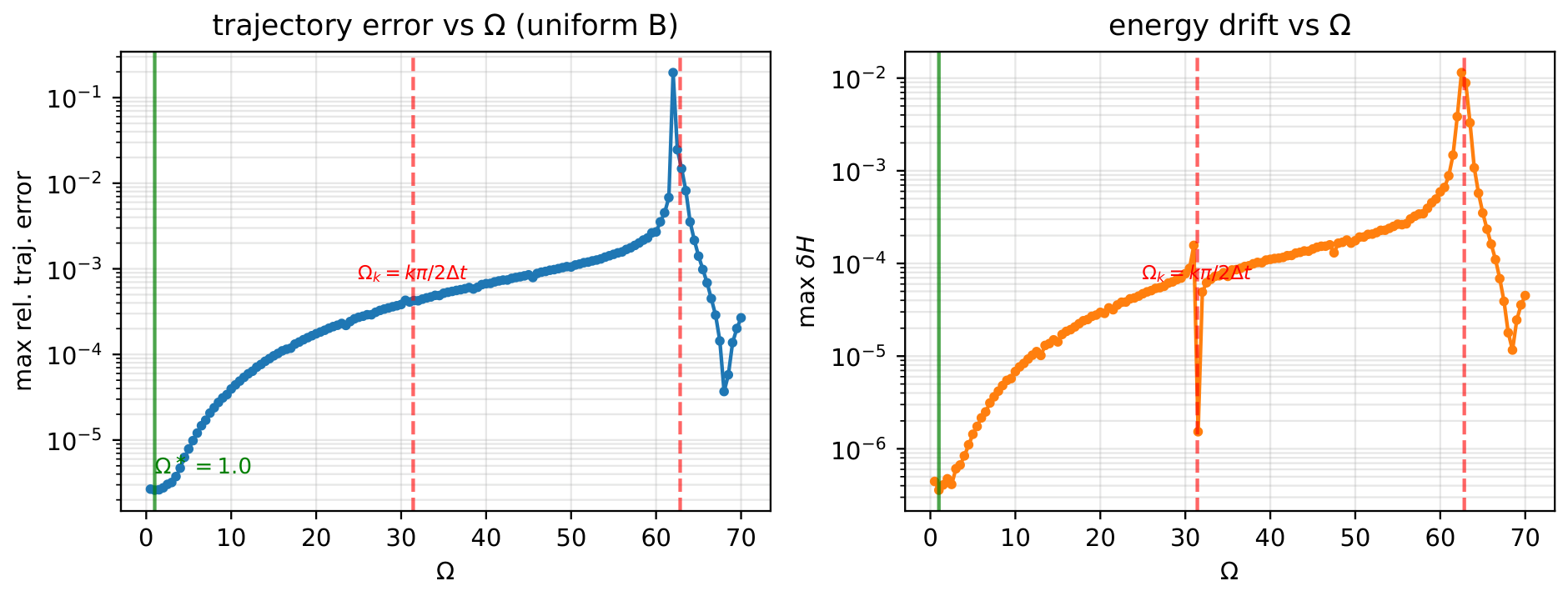
The purpose of the mixed arguments is what makes the non-separable problem explicitly integrable: although ${\mathcal{H}}_{\theta }(\mathbf{r},\mathbf{P})$ couples position and momentum, the copy ${\mathcal{H}}_{\theta }(\mathbf{r},\tilde{\mathbf{P}})$ uses the position of one pair and the momentum of the other, so its Hamiltonian flow updates only the complementary variables $(\tilde{\mathbf{r}},\mathbf{P})$—by an explicit shift (a quadrature), holding $(\mathbf{r},\tilde{\mathbf{P}})$ fixed—and symmetrically for ${\mathcal{H}}_{\theta }(\tilde{\mathbf{r}},\mathbf{P})$. Each of the three pieces (the two mixed copies and the quadratic binding term) therefore has a closed-form symplectic flow. The binding constant $\Omega$ penalizes the two copies drifting apart, so that for large $\Omega$ the synchronized motion $\mathbf{r}\approx \tilde{\mathbf{r}}$, $\mathbf{P}\approx \tilde{\mathbf{P}}$ reproduces the original dynamics up to the binding floor ${\delta }_{\Omega }$; its value must be chosen with care, as that floor depends non-monotonically on $\Omega$ and develops sharp resonances (see Appendix A.2). A symmetric Strang composition of these flows yields a second-order symplectic map ${\Phi }_{\Delta t}^{\left(2\right)}$, which is promoted to fourth order by the Yoshida triple-jump

$${\Phi }_{\Delta t}^{\left(4\right)}={\Phi }_{w_1\Delta t}^{\left(2\right)}\circ {\Phi }_{w_0\Delta t}^{\left(2\right)}\circ {\Phi }_{w_1\Delta t}^{\left(2\right)},w_1={\displaystyle \frac{1}{2-2^{1/3}}},w_0=1-2w_1,$$

(17)

with $w_1\approx 1.3512$, $w_0\approx -1.7024$ [11,12]. All gradients of ${\mathcal{H}}_{\theta }$ are obtained by automatic differentiation. For an autonomous Hamiltonian (the free-particle and magnetic-field cases) the resulting map is exactly symplectic by construction, independently of the accuracy of ${\mathcal{H}}_{\theta }$: even with a small approximation error, the discrete flow is symplectic with respect to ${\mathcal{H}}_{\theta }$. While the Yoshida triple-jump is a fourth-order composition for the extended (binding) Hamiltonian, the order realized for the true trajectory is limited by the binding error of the extended phase space; we measure it directly in Appendix A.2 and find a realized second-order convergence in the coupled limit $\Omega \propto \Delta t^{-1}$. This is consistent with the central message of the paper: the value of the symplectic map is not a higher formal order—a high-order non-symplectic method is more accurate at short times—but the absence of secular error growth. For an explicitly time-dependent Hamiltonian (the Gaussian-pulse case) the field is held fixed at the step time within each composition, so the present implementation is non-autonomously frozen; the exact symplecticity and fourth-order guarantees then apply rigorously only to the static problems, while the laser results in Section 5.2 should be read as those of a high-order structure-aware scheme. Promoting time to a canonical coordinate—extending the phase space by the pair $(t,-\mathcal{H})$ as in Section 2, the momentum canonically conjugate to the time coordinate being $-\mathcal{H}$ (minus the instantaneous energy), with $\mathrm{d}t/\mathrm{d}\tau =1$ under the autonomized flow—restores exact symplecticity for the time-dependent case; we implement this autonomized variant and validate it on a plane wave in Appendix A.1 (Figure A1), where it conserves the light-front (light-cone) invariant $K=\gamma -p_z$—exactly conserved whenever the field depends only on the retarded phase $\eta =z-ct$, as it is the generator of translations along the light front—roughly three orders of magnitude better than the frozen map. The autonomized map is validated on this plane-wave control only; the focused-pulse benchmarks of Section 5.2 use the frozen map, so the three-order improvement is demonstrated on the control rather than deployed in the production figures.

4.4. Surrogate Variant for Time-Dependent Fields: The Vector-Potential Light-Cone Form

For the static (free-particle, magnetic-field, and non-integrable) problems, the surrogate ${\mathcal{H}}_{\theta }$ is learned directly as above. The time-dependent 3+1D laser is substantially harder: the carrier $cos\left[k_0(z-ct)\right]$ produces tens of oscillations across the domain—the spectral bias of plain tanh networks—and the quiver is resonantly forced, so a small force error accumulates into a carrier-phase slip (analyzed in Section 6). For this case, we therefore adopt a lower-dimensional, structurally exact reformulation, which is the configuration behind the learned-pipeline result reported in Section 6. Rather than the seven-dimensional Hamiltonian, the network represents the four-dimensional vector potential in light-cone (light-front) form,

$${\mathbf{A}}_{\theta }(x,y,z,t)={\mathbf{A}}_{\mathrm{pw}}\left(\eta \right)+\mathrm{NN}(x,y,z,t),\eta =z-ct,$$

(18)

with $\eta =z-ct$ the retarded light-front (light-cone) phase for forward, $+z$, propagation, where the analytic plane-wave potential ${\mathbf{A}}_{\mathrm{pw}}\left(\eta \right)$ supplies the carrier exactly and the network learns only the slow focusing correction; the Hamiltonian is then reconstructed analytically as ${\mathcal{H}}_{\theta }=c\sqrt{{(\mathbf{P}-\frac{e}{c}{\mathbf{A}}_{\theta })}^2+m^2{c}^2}$, so the mass-shell constraint holds by construction and the Lorentz force is an exact function of $\partial {\mathbf{A}}_{\theta }$. We stress that this light-cone A-residual is a hybrid physics–machine-learning ansatz: it presupposes the analytic plane-wave part ${\mathbf{A}}_{\mathrm{pw}}\left(\eta \right)$ and is accurate within a near-axis tube about the reference trajectory (a thin neighborhood of the integrated reference orbit, half-widths $[0.4,0.4,0.8,0.8]$ in $(x,y,z,t)$; Appendix A.5), so it is a problem-specific construction—not a universal property of the PINN architecture—whose generality to arbitrary non-stationary fields is correspondingly limited. Training (full hyperparameters in the released code [36]) uses collocation points sampled in a tube around a reference trajectory of the prescribed field—used only to concentrate the sampling domain, not as supervised targets, so the loss remains the unsupervised equation-residual form of Stage 1 and no trajectory data is fitted—together with Fourier features of the carrier phase $\eta$ and a stabilized optimizer—learning-rate warmup, gradient clipping, an upweighted gradient-matching term, residual-based adaptive resampling of the collocation points, and an L-BFGS polish from the best checkpoint. The resulting accuracy and its diagnosis are reported in Section 6.

4.5. Lorentz Symmetry Preservation

Proposition 1

(Mass-shell preservation). Let ${\mathcal{H}}_{\theta }$ satisfy ${\mathcal{H}}_{\theta }=m{c}^2\gamma$ to within ${\epsilon }_{\theta }$, and let the Hamiltonian be autonomous (the free-particle, magnetic-field, and non-integrable cases; the time-dependent laser case is treated by the frozen-in-time map of Section 4 and is excluded here). Then, under the symplectic map ${\Phi }_{\Delta t}$, the invariant $p^{\mu }{p}_{\mu }={({\mathcal{H}}_{\theta }/c)}^2-{\left|\mathbf{p}\right|}^2$ is preserved with a bounded error, with no secular growth. The accounting is regime-dependent: at fixed Ω, the floor is $\mathcal{O}({\epsilon }_{\theta }+{\delta }_{\Omega }+\Delta t^4)$, where ${\delta }_{\Omega }=\mathcal{O}\left({\Omega }^{-1}\right)$ (away from the resonances of Appendix A.2) is the binding floor left by the imperfect synchronization of the two copies; in the coupled limit $\Omega \propto \Delta t^{-1}$ this binding mismatch is instantaneously $\mathcal{O}(\Delta t)$ but oscillatory with vanishing mean over the binding period, so its net effect on the conserved invariant is one order higher, $\mathcal{O}(\Delta t^2)$ (the realized order $r=2$, not 1; Appendix A.2), giving an overall bounded error $\mathcal{O}({\epsilon }_{\theta }+\Delta t^2)$. At fixed Ω the bound holds up to integration times exponentially long in $1/\Delta t$ (the standard backward-error horizon for symplectic maps—finite, though exponentially large); in the coupled limit $\Omega \propto \Delta t^{-1}$, where the modified-Hamiltonian series coefficients themselves become $\Delta t$-dependent, the rigorous guarantee is instead Tao’s algebraically-long averaging horizon $\mathcal{O}(T{\delta }^l\Omega )$ [13]—in both cases a finite (not all-t) time over which there is no secular drift.

Proof. 

The map preserves $\omega$ exactly, hence is a canonical transformation. Backward error analysis for symplectic integrators guarantees that the numerical trajectory lies on the level set of a modified Hamiltonian; strictly this is a modification $\widetilde{\overline{\mathcal{H}}}=\overline{\mathcal{H}}+\mathcal{O}(\Delta t^r)$ of the extended (binding) Hamiltonian on which the map acts, conserved with a bounded, non-accumulating error over times exponentially long in $1/\Delta t$ [10]; projected onto the physical copy—within the binding floor ${\delta }_{\Omega }$ above—this bounds the drift of ${\mathcal{H}}_{\theta }$ to $\tilde{\mathcal{H}}={\mathcal{H}}_{\theta }+\mathcal{O}(\Delta t^r)$, with r examined in Appendix A.2. Hence ${\mathcal{H}}_{\theta }$, and the constraint $p^{\mu }{p}_{\mu }$ derived from it, do not drift secularly. The mass-shell constraint is enforced at training to $\mathcal{O}\left({\epsilon }_{\theta }\right)$, so $p^{\mu }{p}_{\mu }=m^2{c}^2+\mathcal{O}\left({\epsilon }_{\theta }\right)$ initially; combining the two estimates gives the stated bound [10,13]. This bounded behavior—in contrast to the linear-in-N drift of non-symplectic schemes—is exactly what Figure 2 demonstrates.    □

Proposition 2

(Rapidity integral, longitudinal sector). In the purely longitudinal (1+1-dimensional) case ${\mathbf{p}}_{\perp }=0$, where the rapidity $\theta =\mathrm{arcsinh}(p_{\Vert }/mc)$ obeys $\gamma =cosh\theta$, the SP-PINN map satisfies $|{\theta }^n-{\theta }_{\mathrm{exact}}\left(t_n\right)|=\mathcal{O}({\epsilon }_{\theta }+\Delta t^2)$ with bounded, non-secular error (inheriting the coupled-limit assumption of Proposition 1; at fixed Ω a bounded ${\delta }_{\Omega }=\mathcal{O}\left({\Omega }^{-1}\right)$ term adds as there).

We emphasize that the relation $\gamma =cosh\theta$ with $\theta =\mathrm{arcsinh}(p_{\Vert }/mc)$ holds only in the longitudinal sector; in the general 3+1-dimensional case with transverse momentum the genuinely Lorentz-invariant statement is the mass-shell constraint $p^{\mu }{p}_{\mu }=m^2{c}^2$ of Proposition 1, of which $\gamma =cosh\theta$ is the ${\mathbf{p}}_{\perp }=0$ restriction. Proposition 2 then follows from Proposition 1 in that sector. Together, the two propositions establish that the SP-PINN integrator preserves the Lorentz-group orbit structure—the mass hyperboloid $p^{\mu }{p}_{\mu }=m^2{c}^2$—to within errors controlled by the training tolerance ${\epsilon }_{\theta }$ and the time step, in contrast to the unbounded constraint drift of non-symplectic schemes. The same mechanism extends verbatim to the Noether invariants of the spatial point symmetries, which we state once for both the translational and the rotational case.

Proposition 3

(Noether invariants of continuous point symmetries). Suppose the autonomous surrogate Hamiltonian admits a one-parameter point symmetry with Noether invariant $G(\mathbf{q},\mathbf{P})$, i.e., $\{G,{\mathcal{H}}_{\theta }\}=0$; the canonical examples are the transverse translation $G=P_x$ (exact in the plane-wave/broad-beam limit) and the rotation about z, $G=L_z=x{P}_y-y{P}_x$ (exact for an axisymmetric field in the symmetric gauge). Then, under the Stage-2 symplectic map, G is preserved with a bounded, non-secular error $\mathcal{O}({\epsilon }_{\theta }+\Delta t^r)$ over the backward-error horizon of Proposition 1, whereas a non-symplectic scheme lets G drift secularly ($\propto n$).

Proof. 

The map is symplectic with respect to ${\mathcal{H}}_{\theta }$ (up to the extended-phase-space binding floor), so by backward error analysis its iterates lie on the level sets of a modified Hamiltonian $\tilde{\mathcal{H}}={\mathcal{H}}_{\theta }+\mathcal{O}(\Delta t^r)$. Since G is smooth and $\{G,{\mathcal{H}}_{\theta }\}=0$, the Poisson bracket with the modified flow is $\{G,\tilde{\mathcal{H}}\}=\mathcal{O}(\Delta t^r)$; the increment of G per step is thus $\mathcal{O}(\Delta t^r)$ and, being oscillatory with vanishing mean along the modified flow (off resonance), integrates to a bounded fluctuation rather than a secular drift. The surrogate error enters only through $\{G,{\mathcal{H}}_{\theta }-\mathcal{H}\}=\mathcal{O}\left({\epsilon }_{\theta }\right)$, giving the stated bound. A non-symplectic map admits no conserved modified Hamiltonian, so the per-step defect adds coherently and G drifts linearly in the step count—precisely the contrast measured for $P_x$ in the ensemble test of Section 5.2 and for $L_z$ in the rotational test of Section 5.4.    □

These results unify the three symmetry classes exercised in Section 5: the Lorentz symmetry (mass-shell $p^{\mu }{p}_{\mu }$, Proposition 1), the translational symmetry (Noether $P_x$), and the rotational symmetry (Noether $L_z$)—each preserved with bounded, ${\epsilon }_{\theta }$- and $\Delta t$-controlled error by the symplectic stage. The remaining, discrete gauge symmetry is not a Noether invariant but a canonical reparametrization $\mathbf{P}\to \mathbf{P}+\frac{e}{c}\nabla \chi$; the Stage-2 map, being canonical, respects it up to truncation error (the gauge test of Section 5.4), while the learned surrogate is made gauge-consistent by construction through the vector-potential parametrization of Section 4.4.

5. Numerical Experiments

Throughout this section we work in code units ($c=m=k_0={\omega }_0=1$; cf. Table 1), whereas the analytical development of Section 2, Section 3 and Section 4 is written in Gaussian (CGS) units. All experiments were performed in double precision. The CPU computations were carried out with Python 3.13.2, NumPy 2.4.4, SciPy 1.17.1, PyTorch 2.12.0 (CPU build), and Matplotlib 3.10.9; the GPU computations—the throughput benchmark of Section 5.6 and the Stage-1 laser-surrogate training reported in Section 5.8, Section 6, and Appendix A.5—used PyTorch built against CUDA 12.1 on NVIDIA Tesla P100 and T4 GPUs. The complete code is openly available [36] (see Data Availability). The Boris pusher follows the standard relativistic algorithm [3,7] and RK4 is the classical explicit scheme. The Higuera–Cary pusher [5]—a volume-preserving relativistic scheme often preferred over Boris—behaves essentially like Boris on the integrable benchmarks (both reduce to exactly volume-preserving rotations there), so it is shown only in the symplecticity diagnostic of Section 5.7, where it differs from a symplectic map informatively. Throughout this section the curve labeled “SP-PINN” is the Stage-2 explicit symplectic map driven by the analytic relativistic Hamiltonian—that is, the ${\epsilon }_{\theta }\to 0$ idealization of the learned pipeline—so that the figures isolate the geometric properties of the integrator from neural-network approximation error. The realistic training-error floor ${\epsilon }_{\theta }$ of the actual Stage-1 surrogate is reported in Section 5.5; none of the integrator-comparison figures of Section 5.1, Section 5.2, Section 5.3, Section 5.4, Section 5.5, Section 5.6 and Section 5.7 uses the learned surrogate, because at the presently attainable ${\epsilon }_{\theta }\sim 4\times {10}^{-2}$ (static magnetic case) it is not competitive (Section 5.5). The learned Stage-1 surrogate is instead assessed on its own, in Section 5.8 (accuracy across a pulse family), Section 5.9 (the complete learned pipeline on a bunch), and Section 6 (the single-particle learned trajectory). A DOP853 (Dormand–Prince 8(5,3), eighth-order) solver with tight tolerances provides the reference trajectory where an analytic solution is unavailable (for the laser ensemble spectrum, a fine-step integration is used as reference, as noted in Section 5.2). For the laser case the fields $\mathbf{E}=-\frac{1}{c}{\partial }_t\mathbf{A}$ and $\mathbf{B}=\nabla \times \mathbf{A}$ are evaluated by central finite differences of the analytic vector potential, common to all schemes; the resulting field error ($\sim {10}^{-8}$ at the step $h={10}^{-4}$ used) is well below the integrator differences reported in Section 5.2).

5.1. Test Case 1: Uniform Magnetic Field

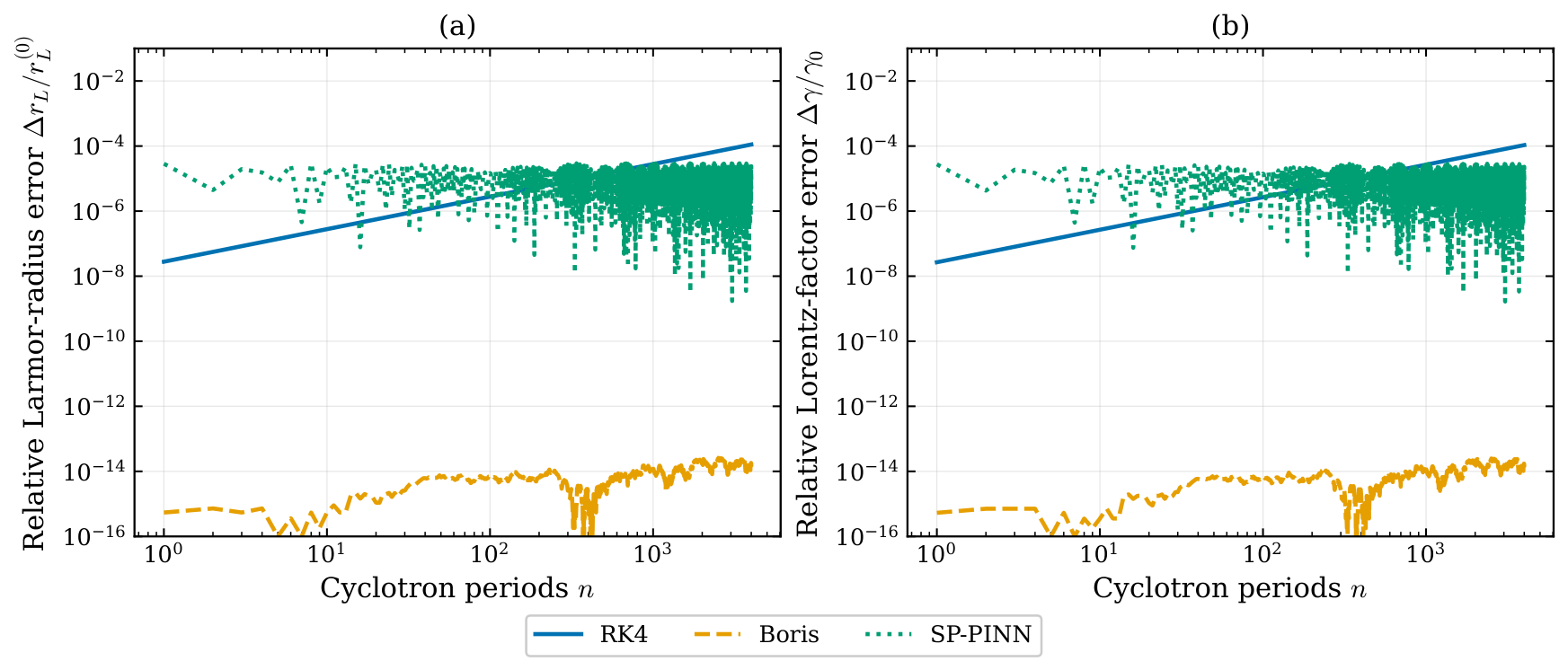
The first case is a relativistic particle in a uniform field $\mathbf{B}=B_0\widehat{\mathbf{z}}$, the prototype integrable relativistic Hamiltonian system. The magnetic force does no work, so the Lorentz factor and the Larmor radius $r_L=p_{\perp }c/\left(e{B}_0\right)$ are exact constants of motion; the cyclotron frequency is ${\omega }_c=e{B}_0/\left(\gamma mc\right)$. We take ${\gamma }_0=5$ (so $p_{\perp }=\sqrt{24}mc$), $p_{\Vert }=0$, and integrate for $4\times {10}^3$ cyclotron periods at $\Delta t=T_c/100$ (the SP-PINN map uses a binding constant $\Omega =15$). At this fixed $\Omega$, the SP-PINN error saturates at a bounded floor rather than converging with $\Delta t$; the realized second-order convergence of the map (Proposition 1) is a distinct property of the coupled limit $\Omega \propto \Delta t^{-1}$, examined separately in Appendix A.2. Figure 2 reports the relative error of the Larmor radius and of the Lorentz factor as functions of the number of gyrations.

Figure 2. Long-term conservation of the exact invariants for a relativistic particle (${\gamma }_0=5$) in a uniform magnetic field over $4\times {10}^3$ cyclotron periods ($\Delta t=T_c/100$, $\Omega =15$), log–log axes. (a) Relative Larmor-radius error $\Delta r_L/r_L^{\left(0\right)}$; (b) relative Lorentz-factor error $\Delta \gamma /{\gamma }_0$, for RK4 (blue, solid), Boris (orange, dashed), and SP-PINN (green, dotted)—each identified by both color and line style. RK4 drifts secularly ($\propto n$, reaching $\sim {10}^{-4}$); Boris conserves both to machine precision (∼${10}^{-14}$) as a volume-preserving gyro-integrator; the symplectic SP-PINN map stays bounded (≲$3\times {10}^{-5}$), overtaking RK4 within a few hundred gyrations. Discussion in Section 5.1.

Figure 2. Long-term conservation of the exact invariants for a relativistic particle (${\gamma }_0=5$) in a uniform magnetic field over $4\times {10}^3$ cyclotron periods ($\Delta t=T_c/100$, $\Omega =15$), log–log axes. (a) Relative Larmor-radius error $\Delta r_L/r_L^{\left(0\right)}$; (b) relative Lorentz-factor error $\Delta \gamma /{\gamma }_0$, for RK4 (blue, solid), Boris (orange, dashed), and SP-PINN (green, dotted)—each identified by both color and line style. RK4 drifts secularly ($\propto n$, reaching $\sim {10}^{-4}$); Boris conserves both to machine precision (∼${10}^{-14}$) as a volume-preserving gyro-integrator; the symplectic SP-PINN map stays bounded (≲$3\times {10}^{-5}$), overtaking RK4 within a few hundred gyrations. Discussion in Section 5.1.

Figure 2 is the textbook contrast between bounded and secular error growth. RK4, being neither symplectic nor volume preserving, accumulates a secular error in both the Larmor radius and the Lorentz factor that grows linearly with the number of gyrations n (the per-step amplitude defect of a non-symplectic Runge–Kutta map applied to rotational motion accumulates coherently, producing the observed $\propto n$ drift). The Boris pusher conserves both invariants to machine precision: for pure gyration, it is an exactly volume-preserving rotation, which is its celebrated property and makes it optimal for this special integrable case [6,8]. The symplectic SP-PINN map keeps the error bounded (≲$3\times {10}^{-5}$) for all time at the level set by the binding tolerance of the extended-phase-space construction; it does not match the machine-precision conservation of Boris on this linear problem, but unlike RK4, it exhibits no secular drift and therefore overtakes RK4 within a few hundred gyrations, ending a few times below it at $n=4\times {10}^3$. This test has a specific scope: on a benign, linear, integrable benchmark, a high-order method such as RK4 is highly accurate at short times, and the Boris pusher is unbeatable for the magnetic sub-problem; the distinctive value of the symplectic SP-PINN scheme is the absence of secular drift together with its applicability to the general non-separable relativistic Hamiltonian, for which exact volume-preserving rotations are not available [9,13,46]. We return to this point in Section 6. We note that Figure 2b is also, directly, a test of mass-shell preservation: in the radiation gauge, the magnetic Hamiltonian is $\mathcal{H}=m{c}^2\gamma$, so the Lorentz norm $p^{\mu }{p}_{\mu }={(\mathcal{H}/c)}^2-{\left|\mathbf{p}\right|}^2=m^2{c}^2$ reduces to ${\gamma }^2-{\left|\mathbf{p}\right|}^2/{\left(mc\right)}^2=1$, and the bounded $\Delta \gamma /{\gamma }_0$ of the symplectic map is exactly the bounded mass-shell error guaranteed by Proposition 1—no secular drift of the mass hyperboloid over the $4\times {10}^3$ gyrations, in contrast to the linear-in-n drift of RK4.

5.2. Test Case 2: Gaussian Laser Pulse (3+1D)

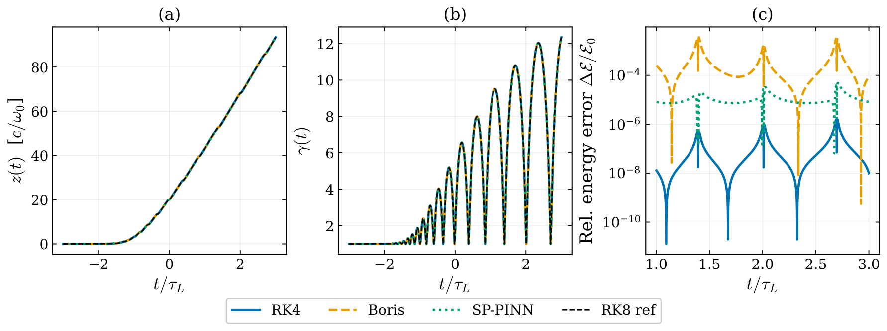
The 3+1-dimensional motion of an electron in the focused Gaussian pulse of Table 1 ($a_0=5$; the Stage-2 map uses a binding constant $\Omega =40$, chosen in a low-error window away from the $\Omega =20,50$ resonances of Appendix A.2). The pulse, centered at $z=ct$, overtakes an electron initially at rest at the origin and drives it forward; once relativistic, the electron co-moves with the pulse and remains within the field over the window shown (still near a carrier peak at the right edge, $t/{\tau }_L=3$), so the strong interaction is not confined to $\left|t\right|\lesssim {\tau }_L$. As discussed in Section 4, for this time-dependent field, the present Stage-2 map is frozen-in-time within each step, so it is here a high-order structure-aware scheme rather than a strictly symplectic one. Consequently, one should not expect SP-PINN to achieve the smallest energy error in this time-dependent case: panel (c) of Figure 3 accordingly shows it lying between RK4 and Boris rather than below both, which is the expected behavior of a frozen (non-strictly-symplectic) map and not a deficiency of the integrator. Figure 3 compares the longitudinal coordinate $z\left(t\right)$, the Lorentz factor $\gamma \left(t\right)$, and the late-time ($t>{\tau }_L$) energy error against the DOP853 reference.

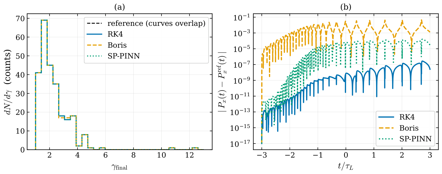
All three integrators reproduce the qualitative dynamics—transverse quiver at the carrier frequency and longitudinal acceleration as the electron is driven forward by and co-moves with the pulse, $\gamma$ oscillating between ≈1 at the carrier troughs and ≈12 at the peaks—and track the reference closely over the moderate interaction window, with RK4 attaining the smallest absolute energy error and SP-PINN remaining within a few $\times {10}^{-5}$ of the reference. Although the Lorentz factor swings violently through the pulse—from $\gamma =1$ at the troughs to $\gamma \approx 12$ at the peaks (Figure 3b)—the mass-shell constraint itself shows no peak-localized drift: in the radiation gauge ($\phi =0$) it reads ${\gamma }^2-{\left|\mathbf{p}\right|}^2/{\left(mc\right)}^2=1$ with $\gamma =\sqrt{1+{\left|\mathbf{p}\right|}^2/{\left(mc\right)}^2}$, and for the learned A-residual surrogate of Section 4.4, the Hamiltonian is reconstructed analytically as ${\mathcal{H}}_{\theta }=c\sqrt{{(\mathbf{P}-\frac{e}{c}{\mathbf{A}}_{\theta })}^2+m^2{c}^2}$, so the constraint holds identically (to machine precision) at every step including through the field peaks, independently of the surrogate error ${\epsilon }_{\theta }$. The surrogate error therefore manifests as a force—and hence trajectory—error (the carrier-phase slip analyzed in Section 6), not as a drift of the mass hyperboloid. Figure 4 examines an ensemble of electrons and the preservation of the transverse translational symmetry. Panel (a) shows the final kinetic-energy spectrum $\mathrm{d}N/\mathrm{d}\gamma$ for 256 electrons with initial transverse positions uniformly distributed in ${[-w_0,w_0]}^2$; all schemes reproduce the reference spectrum closely (mean-energy error below ${10}^{-4}$). Panel (b)—shown to motivate the cleaner plane-wave control of Appendix A.1 rather than as primary evidence—tracks the conserved transverse canonical momentum $P_x=p_x+(e/c)A_x$, the Noether invariant of transverse translations, exactly conserved in the plane-wave limit but only approximately for this finite focused beam (the strict plane-wave control is Appendix A.1), for an on-axis electron, plotting its deviation from the reference. Here, a clear ordering appears, and we are careful not to group the three schemes misleadingly. The Boris pusher violates this Lorentz-related quantity by far the most (up to ∼$4\times {10}^{-2}$); the high-order RK4 is in fact the most accurate here (∼${10}^{-8}$); and the SP-PINN map lies between the two (∼$3\times {10}^{-5}$). That a non-symplectic scheme leads is expected for this time-dependent field, where the present Stage-2 map is frozen-in-time and therefore not strictly symplectic (Section 5.2), so SP-PINN sits at its bounded binding floor rather than at machine precision; the symplectic gain is the bounded, non-secular behavior at long times, which this short finite-window test does not probe. The framing-independent fact is only that the volume-preserving Boris rotation violates this Noether invariant about three orders of magnitude more than the SP-PINN map and far more (around six orders) than RK4. We note a caveat: for the finite focused beam used here ($w_0=5{\lambda }_0$), $P_x$ is conserved only approximately—diffraction weakly breaks the transverse translational symmetry—so panel (b) measures the deviation from the reference trajectory, which conflates a small physical symmetry breaking with numerical error; a strict plane-wave control ($w_0\to \infty$), in which $P_x$ is exactly conserved, isolates the purely numerical violation, and we provide exactly this control in Appendix A.1 (Figure A1b), where the Boris pusher again shows by far the largest, purely numerical, deviation—confirming that the ordering seen here is a numerical effect rather than the residual physical symmetry breaking of the finite beam.

5.3. Test Case 3: A Non-Integrable System

The uniform-field test of Section 5.1 is integrable, and there the Boris pusher is unbeatable; the regime in which symplecticity is genuinely decisive is non-integrable dynamics, where no exact volume-preserving rotation exists. To exhibit this, we consider an autonomous but non-integrable system: a charged particle in a uniform magnetic field $\mathbf{B}=B_0\widehat{\mathbf{z}}$ plus a static anharmonic electrostatic well

$$\phi \left(\mathbf{r}\right)=\frac{1}{2}{k}_{\perp }(x^2+y^2)+ϵx^2{y}^2.$$

(19)

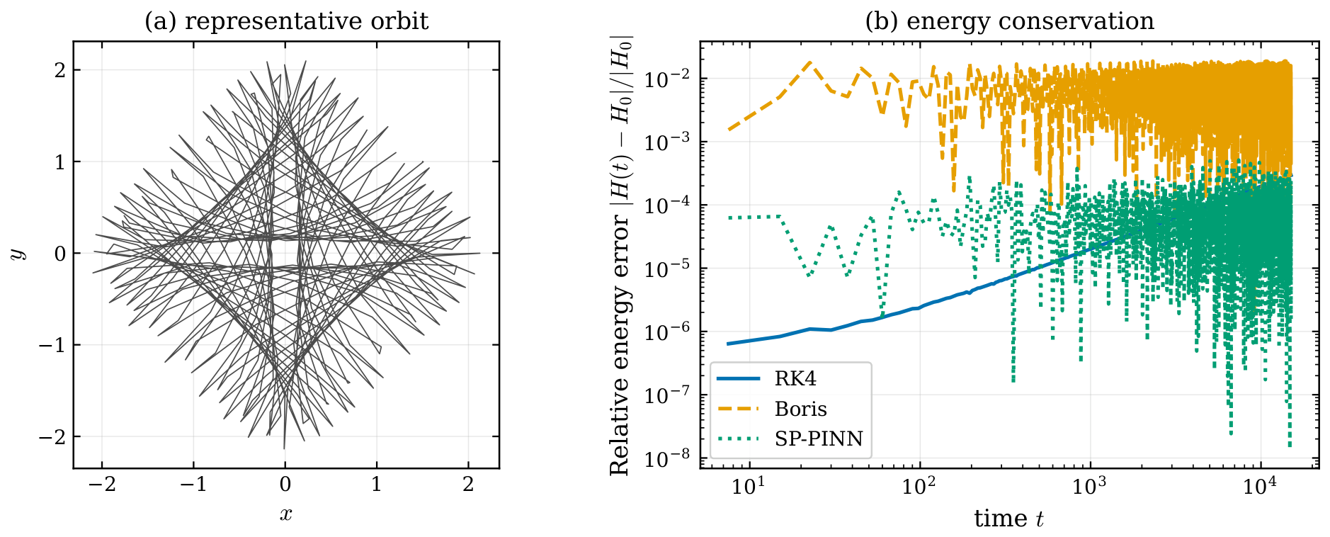
The coupling $ϵx^2{y}^2$ (a Hénon–Heiles-type term) breaks integrability, so the motion is chaotic at moderate energy (Figure 5a), while the total energy $\mathcal{H}=\gamma m{c}^2+e\phi$ is an exact constant of motion. We take $B_0=1$, $k_{\perp }=1$, $ϵ=0.3$, and integrate for $3\times {10}^5$ steps at $\Delta t=0.05$ (the SP-PINN map uses $\Omega =10$). Figure 5b shows the relative energy error: RK4 drifts secularly, the Boris pusher—volume-preserving but not symplectic, and tuned for pure magnetic rotation rather than the nonlinear, inhomogeneous force of the $ϵx^2{y}^2$ coupling, so that (consistent with [6]) its energy error, bounded for the integrable gyration of Section 5.1, grows secularly here—exhibits the largest error, and the symplectic SP-PINN map keeps the energy error bounded for all time. This is the qualitative advantage promised by backward error analysis (Proposition 1), now realized on a system where, unlike the pure gyration of Section 5.1, no scheme can fall back on an exact volume-preserving rotation.

5.4. Test Case 4: Rotational and Gauge Symmetry

The tests so far probe the Lorentz (mass-shell) symmetry and the transverse-translational symmetry (the Noether invariant $P_x$ of Figure 4b). To broaden the symmetry coverage we add two further cases in which the preserved structure is, respectively, a rotational Noether invariant and a gauge symmetry.

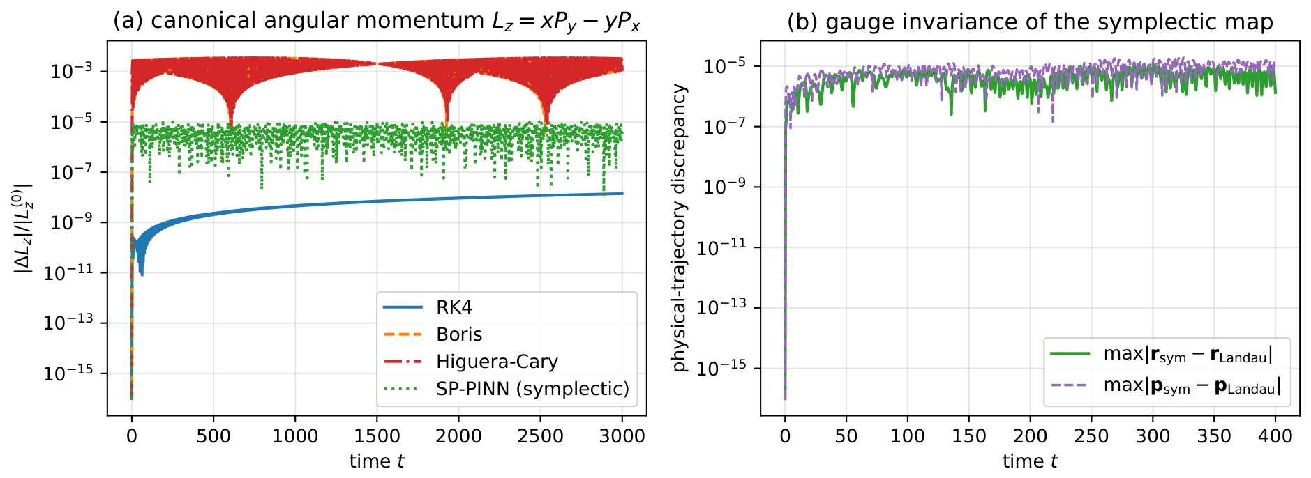
(a) Rotational symmetry. Consider a relativistic particle in a uniform field $\mathbf{B}=B_0\widehat{\mathbf{z}}$ plus an axisymmetric anharmonic well $\phi \left(\rho \right)=\frac{1}{2}{k}_{\perp }{\rho }^2+\beta {\rho }^4$ with ${\rho }^2=x^2+y^2$ ($B_0=k_{\perp }=1$, $\beta =0.05$, positive unit charge). Because the Hamiltonian depends on the transverse coordinates only through $\rho$, it is invariant under rotations about z, and Noether’s theorem makes the canonical angular momentum $L_z=x{P}_y-y{P}_x$ an exact constant of motion (in the symmetric gauge, where $L_z$ generates the rotation; the kinetic angular momentum $x{p}_y-y{p}_x=L_z-\frac{e}{2c}{B}_0{\rho }^2$ is not conserved). We integrate an off-axis orbit (${\mathbf{r}}_0=(1.5,0,0)$, ${\mathbf{p}}_0=(0.10,0.80,0.20)$, so $L_z^{\left(0\right)}=2.325$) for $1.2\times {10}^5$ steps ($\Delta t=0.025$, $\Omega =15$) and track the drift of $L_z$ (Figure 6a). The volume-preserving but non-symplectic Boris and Higuera–Cary pushers, operating here against a nonlinear radial force, show the largest drift of the canonical invariant (∼${10}^{-3}$, with a secular late-time slope ∼$4\times {10}^{-7}$), exactly as they did for $P_x$ in Figure 4b; the symplectic SP-PINN map holds $L_z$ at a bounded floor (≲$5\times {10}^{-6}$, slope $\sim 4\times {10}^{-10}$, i.e., essentially flat), while the high-order RK4 is very accurate over this interval (as on the $P_x$ test), carrying no structural guarantee of remaining so at longer times. The ordering—non-symplectic volume-preserving schemes worst on the Noether invariant, the symplectic map bounded—mirrors the translational case and confirms that the structure preservation is not specific to one symmetry.

(b) Gauge symmetry. The same physics expressed in two gauges—symmetric $\mathbf{A}=\frac{1}{2}{B}_0(-y,x,0)$ and Landau $\mathbf{A}=(-B_{0}y,0,0)$—has identical fields $\mathbf{E},\mathbf{B}$ and hence an identical physical trajectory $(\mathbf{r},\mathbf{p})$. The Boris/RK4/Higuera–Cary pushers use only $\mathbf{E},\mathbf{B}$ and are gauge invariant by construction; only the canonical Stage-2 map sees the gauge, through ${\mathcal{H}}_{\theta }$ and the canonical momentum $\mathbf{P}=\mathbf{p}+\frac{e}{c}\mathbf{A}$. Integrating the same physical initial condition through the symplectic map in the two gauges yields physical trajectories that agree to ${max}_t|{\mathbf{r}}_{\mathrm{sym}}-{\mathbf{r}}_{\mathrm{Landau}}|\approx 1.1\times {10}^{-5}$ and ${max}_t|{\mathbf{p}}_{\mathrm{sym}}-{\mathbf{p}}_{\mathrm{Landau}}|\approx 1.9\times {10}^{-5}$ over $t\in [0,400]$ (Figure 6b)—set by the integrator’s own truncation and orders of magnitude below the inter-scheme spread of panel (a). The canonical map is therefore gauge invariant up to discretization error, as it must be: a gauge transformation $\mathbf{A}\to \mathbf{A}+\nabla \chi$ is a canonical transformation of $\mathbf{P}$ that leaves the symplectic form and the physical observables unchanged. (The learned laser surrogate of Section 4.4 is built in the same gauge-consistent way, learning the vector potential ${\mathbf{A}}_{\theta }$ and reconstructing ${\mathcal{H}}_{\theta }$ analytically.)

5.5. Computational Cost

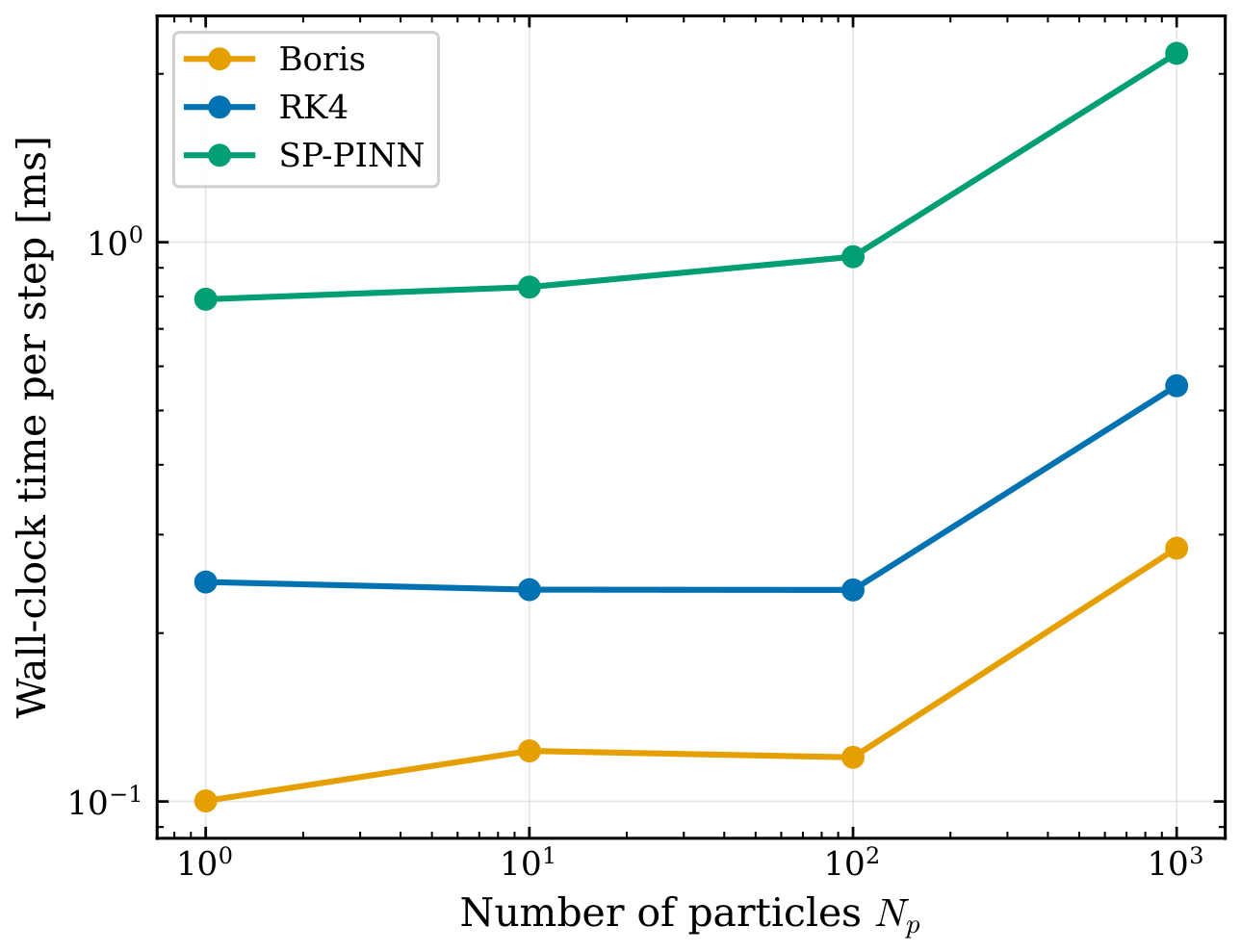
Figure 7 reports the total wall-clock time per integration step as a function of the number of particles integrated in parallel (batched NumPy), measured on the magnetic-field problem. Per single particle (mean ± standard deviation over five trials), Boris is cheapest ($0.108\pm 0.003$ ms), RK4 intermediate ($0.217\pm 0.004$ ms), and the SP-PINN symplectic map most expensive ($0.726\pm 0.004$ ms), because each step evaluates the Hamiltonian gradients several times within the Yoshida composition. The total per-step time grows sublinearly with the batch size, so the per-particle cost decreases under batching—to ≈$2.2\times {10}^{-3}$ ms for SP-PINN at $N_p={10}^3$—but the cost ratio stays roughly constant (≈$7\times$ versus Boris and ≈$3\times$ versus RK4) across all batch sizes; the symplectic map is, and remains, several times more expensive per particle. These figures are single-CPU; one might expect a GPU to narrow the ratio, since the dominant per-step cost—the several automatic-differentiation evaluations of $\nabla {\mathcal{H}}_{\theta }$ inside the Yoshida composition—maps onto the highly parallel batched tensor kernels for which PyTorch is optimized, whereas the Boris rotation is arithmetically minimal and benefits less from parallelism. For the PIC-style workloads that motivate this work—many particles pushed simultaneously—we now report a dedicated GPU benchmark in Section 5.6. It shows that the GPU exposes a bounded, ensemble-size-independent constant factor (≈$14\times$ versus Boris in double precision) at a high absolute throughput ($2\times {10}^7$ symplectic particle-steps per second), fully amortized under batching—not a scaling penalty. We are explicit that this constant ratio does not fall below the single-CPU figure: removing the framework overhead simply exposes the true arithmetic ratio, which the single-CPU timing had compressed. The relevant point for PIC workloads is that the overhead is a fixed multiple, independent of the number of particles. The one-time Stage-1 training of the PINN surrogate is a fixed offline cost. Training the compact network of Section 4 on the magnetic-field Hamiltonian over the domain $\mathbf{r},\mathbf{P}\in {[-6,6]}^3$ for about $3.5$ min per seed on a single CPU (an Intel Core i7-4770; 2500 Adam epochs followed by 80 L-BFGS iterations) reaches, over five random seeds, a root-mean-square test error of only ${\epsilon }_{\theta }=(4.1\pm 0.5)\times {10}^{-2}$ in ${\mathcal{H}}_{\theta }$ and its gradients, with a larger worst-case error (∼$0.3$) near the domain boundary. This surrogate accuracy—not the geometric integrator—is the present bottleneck of the fully learned pipeline: at ${\epsilon }_{\theta }\sim 4\times {10}^{-2}$ the learned-Hamiltonian integration does not yet match the conventional pushers, and the headline curves of Figure 2, Figure 3 and Figure 4 accordingly use the analytic Hamiltonian, i.e., the ${\epsilon }_{\theta }\to 0$ limit. Driving ${\epsilon }_{\theta }$ down for the full 3+1D surrogate—primarily by reformulating what the network represents (the vector-potential light-cone form of Section 6), together with adaptive collocation and improved optimization rather than raw network size—is the principal direction of ongoing work. Representative timings are collected in

Table 2. Computational cost and long-time conservation summary (magnetic-field test, single CPU). Wall-clock time per step is measured for a single particle; under batched evaluation of $N_p={10}^3$ particles the per-particle cost of SP-PINN falls to ≈$2.2\times {10}^{-3}$ ms (Figure 7). The SP-PINN Stage-1 training is a one-time offline cost. Conservation entries refer to the long-time behavior of Figure 2; the learned-${\mathcal{H}}_{\theta }$ row reports the per-step cost (identical to the analytic map, plus a network forward pass) together with the estimated long-time error floor $\sim {\epsilon }_{\theta }$, not a separate long-time benchmark.

Integrator	Symplectic	Time/Step (ms)	Larmor Radius	Lorentz Factor
Boris	no (volume-pres.)	$0.11$	machine precision	machine precision
RK4	no	$0.22$	secular drift	secular drift
SP-PINN (analytic $\mathcal{H}$)	yes	$0.73$	bounded	bounded
SP-PINN (learned ${\mathcal{H}}_{\theta }$, estimated)	yes	$0.73$	floor $\sim {\epsilon }_{\theta }$	floor $\sim {\epsilon }_{\theta }$

.

For the vector-potential surrogate of Section 4.4 the Hamiltonian is not predicted by a network head but reconstructed in closed form from the learned ${\mathbf{A}}_{\theta }$ as ${\mathcal{H}}_{\theta }=c\sqrt{{(\mathbf{P}-\frac{e}{c}{\mathbf{A}}_{\theta })}^2+m^2{c}^2}$. This reconstruction is a handful of floating-point operations and is negligible against the dominant per-step cost—the automatic-differentiation evaluation of the network and of the spatial gradients $\partial {\mathbf{A}}_{\theta }$ that supply the Lorentz force, which is 7–$20\times$ more expensive than the closed-form analytic gradient (Section 5.6). Reconstructing $\mathcal{H}$ analytically rather than predicting it directly therefore costs essentially nothing yet enforces the mass-shell exactly by construction (Section 5.2).

The figure of merit for long campaigns is not raw speed but accuracy per unit cost, and it is most informative in the non-integrable regime the method targets.

Table 3. Cost-weighted long-time accuracy on the non-integrable trap (Section 5.3) at the Figure 5 horizon ($t=1.5\times {10}^4$). The relative energy error $\delta \mathcal{H}$ is the late-time mean over the final quarter of the run; “accuracy per cost” is $1/[\delta \mathcal{H}\times (\mathrm{time}/\mathrm{step}\left)\right]$, normalized to Boris. The Tao map gives the best accuracy-per-cost despite the highest per-step cost, and is the only bounded (non-secular) entry. Entries are from a single representative chaotic orbit; the robust, realization-independent feature is the trend—the late-time per-step drift slope is ∼$2\times {10}^{-7}$ (Boris) and ∼$5\times {10}^{-9}$ (RK4) versus ≈0 for the bounded Tao map—rather than the precise factor, which varies with initial conditions. Because the secular methods’ error grows with the horizon, the near-parity of the Tao (16) and RK4 (15) figures at this finite horizon understates the asymptotic advantage of the bounded map—only Tao’s accuracy-per-cost is horizon-independent. Single CPU.

Integrator	Time/Step (ms)	$\mathit{\delta }\mathcal{H}$ (Late)	Long-Time Trend	Accuracy/Cost (Rel.)
Boris	$0.11$	$7.5\times {10}^{-3}$	secular	1
RK4	$0.22$	$2.6\times {10}^{-4}$	secular ($\times 7$)	15
SP-PINN (Tao)	$0.73$	$7.1\times {10}^{-5}$	bounded	16

reports it on the chaotic trap of Section 5.3 at the horizon of Figure 5 ($3\times {10}^5$ steps, $t=1.5\times {10}^4$), defined as the inverse of the cost-weighted long-time energy error $\delta \mathcal{H}\times \left(\mathrm{wall}\text{-}\mathrm{time}\mathrm{per}\mathrm{step}\right)$ and normalized to the Boris pusher. Despite its ≈$7\times$ per-step cost, the symplectic Tao map attains the best accuracy-per-cost—about $16\times$ that of Boris and marginally above high-order RK4—because in this non-integrable regime its bounded energy error (∼$7\times {10}^{-5}$, late-time mean) undercuts the secular drift of Boris (∼$8\times {10}^{-3}$) and of RK4 (∼$3\times {10}^{-4}$, having grown ≈$7\times$ over the run). Crucially, only the Tao entry is non-secular, so its margin over RK4—comparable at this horizon—widens without bound as the integration lengthens; on the integrable magnetic case of Section 5.1, by contrast, the volume-preserving Boris pusher remains unbeatable at machine precision. The accuracy-per-cost advantage of the symplectic map is thus specific to the non-separable, non-integrable regime it is designed for, not a universal speed claim.

5.6. GPU Throughput of the Symplectic Map

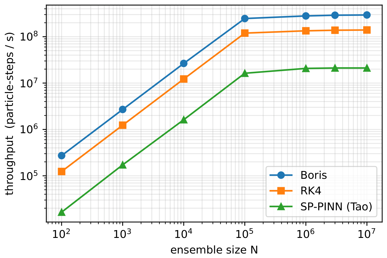
The single-CPU cost ratios of Section 5.5 left open the GPU behavior that PIC workloads require. We therefore implemented all three pushers as batched tensor kernels and measured their throughput, in double precision, on an NVIDIA Tesla P100, as a function of the ensemble size $N_p$ (Figure 8). Throughput saturates above $N_p\approx {10}^5$ at $2.95\times {10}^8$ (Boris), $1.40\times {10}^8$ (RK4), and $2.12\times {10}^7$ (SP-PINN) particle-steps per second. The key observation is that the SP-PINN/Boris overhead is a bounded, $N_p$-independent constant factor (≈$14\times$ in double precision, ≈$6.6\times$ relative to RK4), not a scaling penalty: it reflects the fixed number of Hamiltonian-gradient evaluations per step in the Yoshida composition (three sub-steps, each with several force evaluations) and is fully amortized under batching. We deliberately do not claim that the GPU narrows the gap below the CPU ratio—on the contrary, the GPU exposes the true arithmetic ratio, which the single-CPU framework overhead had compressed—but the absolute throughput ($2\times {10}^7$ particle-steps/s for the symplectic map) is high, and Boris and Higuera–Cary cannot integrate a learned, non-separable Hamiltonian at all, so for the learned pipeline the relevant comparison is structure preservation per unit cost rather than raw speed. For the learned surrogate specifically, the per-step gradient $\nabla {\mathcal{H}}_{\theta }$ obtained by automatic differentiation of the trained network is 7–$20\times$ more expensive than the closed-form analytic gradient (single-CPU, batch sizes 1–${10}^4$), quantifying the framework overhead of the learned-${\mathcal{H}}_{\theta }$ row of Table 2.

5.7. Direct Measurement of the Poincaré–Cartan Invariant; A Structure-Preserving Comparator

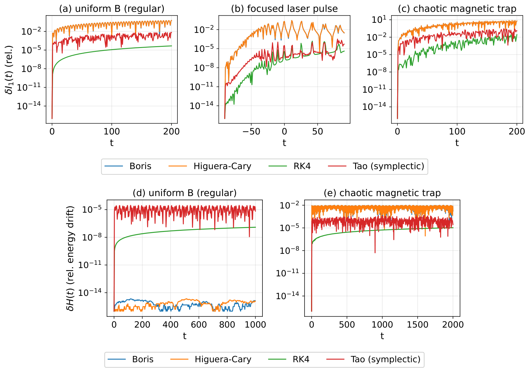
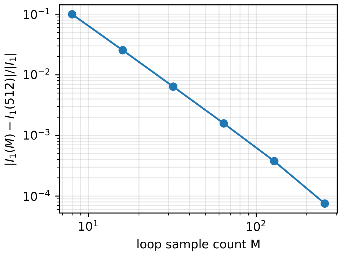
Symplecticity is the central claim of the method, yet the main-text figures track energy and the Larmor radius rather than the loop invariant itself. We close this gap by computing the first Poincaré integral invariant $I_1={\oint }_{\mathcal{C}}\mathbf{P}·\mathrm{d}\mathbf{q}$ directly, transporting a closed loop of $M=256$ phase-space points (a small circle in the $(x,P_x)$ plane) under each integrator and measuring its relative drift $\delta I_1\left(t\right)$ (Figure 9a–c). The midpoint loop quadrature of Equation (10) converges super-algebraically in M for a smooth periodic loop—the Euler–Maclaurin boundary terms cancelling by periodicity—as the small transported circle used here remains over the diagnostic window, so the diagnostic is itself well resolved at $M=256$: doubling the loop resolution to $M=512$ changes the measured $I_1$ by only $7.5\times {10}^{-5}$ (relative; i.e., below $0.01\%$), the reduction accelerating with M (a relative change of $3.8\times {10}^{-4}$ already at $M=128\to 256$, a factor $\approx 5$ per doubling); the reported $\delta I_1\left(t\right)$ is therefore insensitive to the choice $M=256$ (loop-quadrature convergence data at the end of Appendix A.3). As an additional, modern structure-preserving baseline, we also include the Higuera–Cary pusher [5]—a volume-preserving relativistic scheme often preferred over Boris—implemented as the Boris rotation with the future-consistent ${\gamma }^{+}$ of the Higuera–Cary quadratic.

The two diagnostics together sharpen the bounded-versus-secular picture and the distinction between volume preservation and symplecticity. For the uniform field, the Tao map keeps $\delta I_1$bounded and, at fixed $\Omega$, converging as $\mathcal{O}(\Delta t^4)$ (the realized order on the trajectory is second in the coupled limit $\Omega \propto \Delta t^{-1}$; Appendix A.3), whereas Boris and Higuera–Cary—volume preserving but not symplectic—drift secularly in the canonical loop invariant, the per-step loop-area defect $\mathcal{O}(\Delta t)$ accumulating to a relative drift of order $0.6$ over the run at $\Delta t=0.05$, even though they conserve the energy of the same orbit to machine precision (Figure 9d). This is exactly the volume-preserving-but-not-symplectic signature: the standard pushers preserve phase-space volume and energy yet not the symplectic two-form. In the chaotic trap of Section 5.3, the energy drift is the decisive diagnostic: over $t=2000$ (this shorter diagnostic horizon; cf. the longer $t=1.5\times {10}^4$ production run of Figure 5 and Table 3, where the Tao floor is ∼$7\times {10}^{-5}$) the Tao map holds $\delta \mathcal{H}\sim 3\times {10}^{-5}$ (bounded, non-secular), while Boris and Higuera–Cary drift secularly to ∼${10}^{-2}$—about $2.5$ orders larger (Figure 9e). Consistent with the honest framing of Section 6, the high-order non-symplectic RK4 remains competitive in magnitude on the smooth integrable orbit; the symplectic signature is the bounded (non-secular) behavior, decisive in the chaotic regime and in the symplectic two-form.

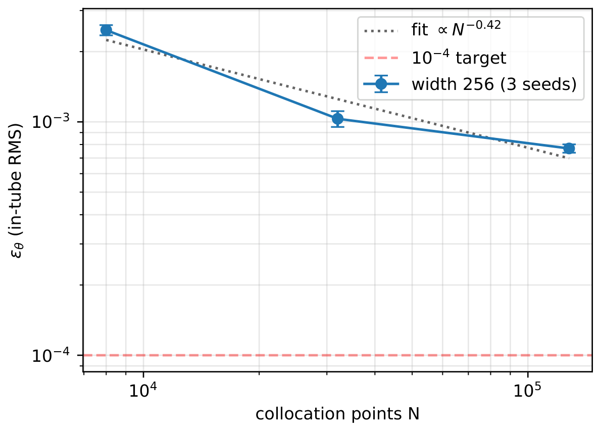
5.8. One Surrogate for a Pulse Family

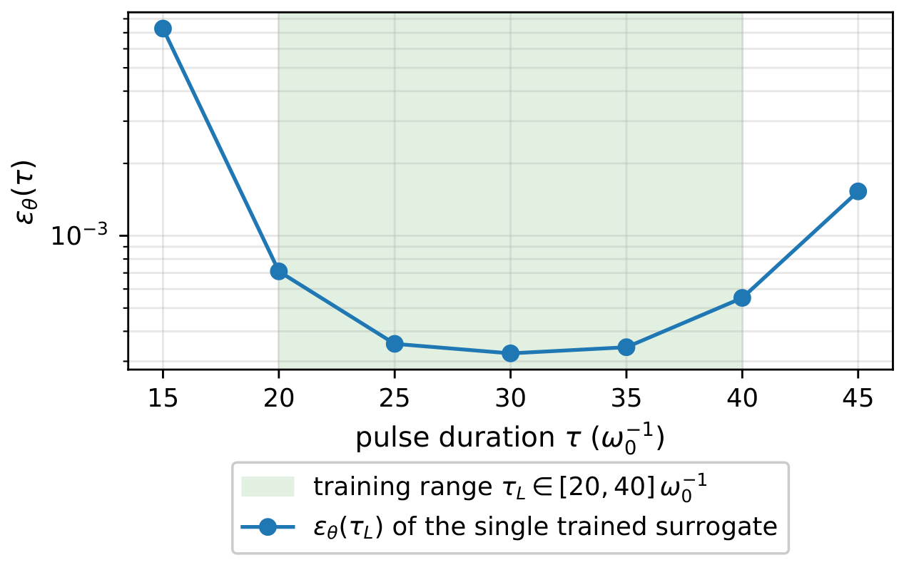
The surrogate of Section 5.2 is trained for a single pulse. A genuine framework should learn a family. We therefore trained one network on the pulse-duration parameter ${\tau }_L$, taking the A-residual form of Section 4.4 with ${\tau }_L$ adjoined as an input, $A_{\theta }(x,y,z,t;{\tau }_L)$, and sampling collocation points jointly with ${\tau }_L\in [20,40]{\omega }_0^{-1}$ (the amplitude $a_0$ is excluded because $\mathbf{A}\propto a_0$ exactly, so generalization in $a_0$ is trivial). The network architecture, tube geometry (half-widths $[0.4,0.4,0.8,0.8]$ in $x,y,z,t$), and optimizer match the single-pulse surrogate of Appendix A.5, with ${\tau }_L$ adjoined as a fifth input and the collocation budget set to $N_{\mathrm{coll}}=2\times {10}^5$ points (sampled jointly over the tube and the ${\tau }_L$ band) trained for $2.5\times {10}^4$ Adam epochs followed by an L-BFGS polish—i.e., the single-pulse recipe with one extra input dimension. The resulting single network reaches ${\epsilon }_{\theta }=3.2\times {10}^{-4}$ at ${\tau }_L=30$—matching the single-pulse surrogate—and stays in the range $(3$–$7)\times {10}^{-4}$ across the whole trained band, with graceful degradation under extrapolation (${\epsilon }_{\theta }\approx 7\times {10}^{-3}$ at ${\tau }_L=15$ and $1.5\times {10}^{-3}$ at ${\tau }_L=45$); see Figure 10. Thus the symmetry-constrained surrogate generalizes across a continuous family of pulses at no loss of in-band accuracy, supporting the framework reading of the method rather than a single-instance fit.

5.9. Ensemble-Level Structure Preservation with the Learned Pipeline

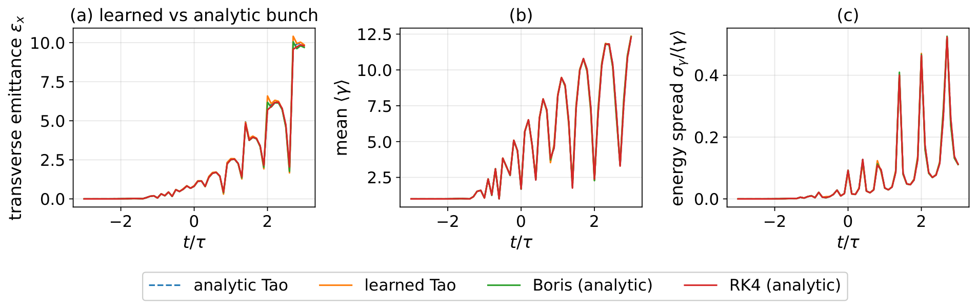
Finally, we exercise the complete learned pipeline (learned $A_{\theta }$ advanced by the Stage-2 Tao map) on a bunch of $N_p=2500$ electrons in the focused pulse, comparing against the analytic-$\mathcal{H}$ Tao reference (the ${\epsilon }_{\theta }\to 0$ limit) and the Boris/RK4 pushers. For a cold bunch that remains within the surrogate’s training tube, the learned pipeline reproduces the analytic bunch evolution to better than one percent in every observable: the final transverse emittance agrees to $0.25\%$, the mean Lorentz factor to $0.58\%$, the energy spread to $0.65\%$, and the final energy spectrum to a Kolmogorov–Smirnov distance of $0.026$ (Figure 11); all four integrators give a physical $\langle \gamma \rangle \approx 12$ and overlapping trajectories. This demonstrates the learned two-stage framework at the ensemble (PIC-relevant) scale. We note the expected limitation that this test also makes precise: the A-residual surrogate is a near-axis ansatz (Section 4.4), valid only within the tube around the reference trajectory; a hot or wide bunch whose particles are driven off-axis by the $a_0=5$ quiver leaves the tube, where the surrogate extrapolates, so quantitative agreement at the bunch level presently requires a cold, near-axis bunch. This test is therefore a proof-of-concept of collective structure preservation, not a production bunch-tracking claim; extending it to a warm or wide bunch amounts to training on a correspondingly wider tube, and characterizing the resulting trade-off between ${\epsilon }_{\theta }$ and tube width is a separate study deferred to future work (Section 6)—not a prerequisite for the single-particle results that are the subject of this paper.

6. Discussion

6.1. Symplecticity Versus Volume Preservation

The central lesson of Section 5 is the distinction between bounded and secular error growth, and the complementary roles of the three integrators. A common simplification in the particle-pushing literature equates energy conservation, volume preservation, and symplecticity [6]; the magnetic-field test makes the distinctions concrete. The Boris pusher is exactly volume preserving for pure gyration and conserves the Larmor radius and Lorentz factor to machine precision, making it the method of choice for the magnetic sub-problem; it is, however, not symplectic in the strict sense, and its favorable behavior does not automatically extend to general non-separable fields [6,9]. RK4 is highly accurate at short times but drifts secularly, because its discrete map is not structure preserving. The symplectic SP-PINN map, through backward error analysis, keeps the error bounded for all time and therefore overtakes RK4 at long integration times. We deliberately avoid overstating the magnitude of the advantage on this benign, integrable benchmark: a high-order non-symplectic method is competitive here, and the symplectic gain is qualitative (bounded versus secular) rather than a dramatic short-time accuracy improvement. The regime in which symplecticity becomes decisive is long-time integration and non-integrable dynamics in complex fields, where no exact volume-preserving rotation is available and where secular drift of non-symplectic schemes dominates the error budget [9,10,49]. The principal practical contribution of SP-PINN is to make explicit, structure-preserving integration available for the general non-separable relativistic Hamiltonian through the learned surrogate, rather than to outperform Boris on the special magnetic case.

6.2. Role of the Mass-Shell Constraint

The mass-shell term ${\mathcal{L}}_{\mathrm{constraint}}={({\mathcal{H}}_{\theta }-m{c}^2\gamma )}^2$, weighted by ${\lambda }_1\gg 1$, is the design choice intended to carry Lorentz-symmetry preservation in the direct-Hamiltonian surrogate: enforcing it throughout training is expected to bias the learned Hamiltonian toward the mass-hyperboloid geometry, whereas omitting it lets the surrogate fit the equations of motion while $p^{\mu }{p}_{\mu }$ drifts. We isolate this term directly (

Table 4. Ablation of the mass-shell loss term on the static magnetic surrogate (mean ± standard deviation over three seeds; identical configuration, 2500 Adam $+80$ L-BFGS iterations, $N_{\mathrm{coll}}=4000$, domain ${[-6,6]}^3$, code units $c=m=1$; local_massshell_ablation.py). Removing the term (${\lambda }_1=0$) leaves only the equations-of-motion gradient loss. The dynamics (the gradients the integrator consumes) are fit at least as well without the term, but the surrogate energy value—and hence the Lorentz mass shell $p^{\mu }{p}_{\mu }=m^2{c}^2$—then drifts by ∼$2.5$ orders of magnitude. The de-meaned mass-shell residual (last row) shows the drift is a genuine non-uniform excursion, not a removable constant offset. Here, ${\epsilon }_{\theta }$ is the largest of the three RMS errors (the value error dominates in both columns); in code units ($c=m=1$), $m{c}^2\gamma \sim 1$–5 over the domain, so the bare magnitudes ($21.9$, 222) are several times to ∼$200\times$ the local energy/mass-shell scale.

Quantity (RMS)	with (${\mathit{\lambda }}_1=10$)	Without (${\mathit{\lambda }}_1=0$)	Factor
${\mathcal{H}}_{\theta }$ error vs. $m{c}^2\gamma$ ($={\epsilon }_{\theta }$)	$(4.1\pm 0.6)\times {10}^{-2}$	$21.9\pm 0.1$	∼$500\times$
$\partial {\mathcal{H}}_{\theta }/\partial \mathbf{P}$ error (dynamics)	$3.2\times {10}^{-2}$	$2.5\times {10}^{-3}$	$0.08\times$
$\partial {\mathcal{H}}_{\theta }/\partial \mathbf{r}$ error (dynamics)	$1.4\times {10}^{-2}$	$1.2\times {10}^{-3}$	$0.09\times$
mass-shell residual $|p^{\mu }{p}_{\mu }-m^2{c}^2|$	$0.49$	222	∼$450\times$
same, de-meaned	$0.49$	88	∼$180\times$

): the static magnetic surrogate is trained identically except for the mass-shell weight—${\lambda }_1=10$ (with) versus ${\lambda }_1=0$ (the equations-of-motion gradient loss alone)—over three seeds. The result confirms the term’s role and sharpens it. Removing the mass-shell term does not harm the dynamics: the gradient errors $\parallel \partial {\mathcal{H}}_{\theta }/\partial \mathbf{P}-\dot{\mathbf{r}}\parallel$ and $\parallel \partial {\mathcal{H}}_{\theta }/\partial \mathbf{r}+\dot{\mathbf{P}}\parallel$—the quantities the integrator actually consumes—are in fact smaller without it (by about $13\times$), since all network capacity is spent on the equations-of-motion residual. What collapses is the value of the surrogate Hamiltonian, and with it the mass shell: ${\mathcal{H}}_{\theta }$ departs from $m{c}^2\gamma$ by ≈22 (versus ${\epsilon }_{\theta }=(4.1\pm 0.6)\times {10}^{-2}$ with the term—a factor $\sim 500$), and the RMS mass-shell residual $|p^{\mu }{p}_{\mu }-m^2{c}^2|$ rises from $0.49$ to 222 (a factor $\sim 450$). This is precisely the expected mechanism: Hamilton’s equations determine ${\mathcal{H}}_{\theta }$ only up to an additive constant, so the gradient loss alone is blind to the energy value, and only the mass-shell term anchors the surrogate to the Lorentz hyperboloid. That the departure is a genuine non-uniform excursion off the hyperboloid rather than a removable constant offset is confirmed by the de-meaned residual, itself ≈88 without the term (∼$180\times$ the constrained value); de-meaning removes only the exact additive zero-mode, so this also rules out a slowly-varying, low-gradient drift mode that the sampled gradients would otherwise leave weakly determined. The mass-shell constraint is therefore, as claimed, the ingredient that keeps the direct surrogate on the mass hyperboloid—now measured, not merely asserted, and consistent with the broader experience that high-weight constraint residuals improve the geometric fidelity of constrained-Hamiltonian PINNs [23,51], including recent structure-preserving and constrained (Hamilton–Dirac) formulations [53,54]. Moreover, in our best learned configuration—the A-residual laser surrogate of Section 4.4—the mass shell is enforced analytically, by the closed-form reconstruction ${\mathcal{H}}_{\theta }=c\sqrt{{(\mathbf{P}-\frac{e}{c}{\mathbf{A}}_{\theta })}^2+m^2{c}^2}$, so there the trained ${\mathcal{L}}_{\mathrm{constraint}}$ is bypassed entirely and the symmetry preservation comes from the architecture rather than the loss. The mass-shell loss is thus the symmetry mechanism for the direct surrogate, while the demonstrated laser result owes its mass-shell exactness to the analytic reconstruction.

6.3. Limitations

Several limitations deserve emphasis. First, and most importantly, the surrogate ${\mathcal{H}}_{\theta }$ has so far been trained only for the static magnetic-field Hamiltonian, where it reaches only ${\epsilon }_{\theta }=(4.1\pm 0.5)\times {10}^{-2}$ (root-mean-square over the training domain, five seeds) with about $3.5$ min of single-CPU training per seed; at this accuracy the learned pipeline is not competitive with conventional pushers, which is why every figure here uses the analytic Hamiltonian in Stage 2. Training a surrogate for the time-dependent 3+1D laser Hamiltonian is markedly harder still, and exposes a sharper obstacle: a plain tanh network over the full phase-space–time box fails to learn it, because the laser carrier $cos\left[k_0(z-ct)\right]$ produces tens of oscillations across the domain that the network cannot represent—the well-known spectral bias of multilayer perceptrons. With a plain network the loss stalls near ${\epsilon }_{\theta }\approx 0.8$ and the resulting Hamiltonian yields trajectories whose amplitude is wrong by a factor of two. This obstacle is substantially mitigated by (i) sampling collocation points in a tube around the integrated trajectory, concentrating capacity where the integrator evaluates ${\mathcal{H}}_{\theta }$, and (ii) augmenting the input with Fourier features of the carrier phase $\eta =z-ct$. On a single GPU, these two changes restore healthy training (the loss falls by four orders of magnitude rather than stalling) and reduce the in-tube error to ${\epsilon }_{\theta }\approx 9\times {10}^{-3}$ (root-mean-square; worst case $\sim 0.7$ near the tube boundary), recovering the correct trajectory amplitude (peak $\gamma \approx 12$); the learned trajectory tracks the exact one closely early in the interaction.

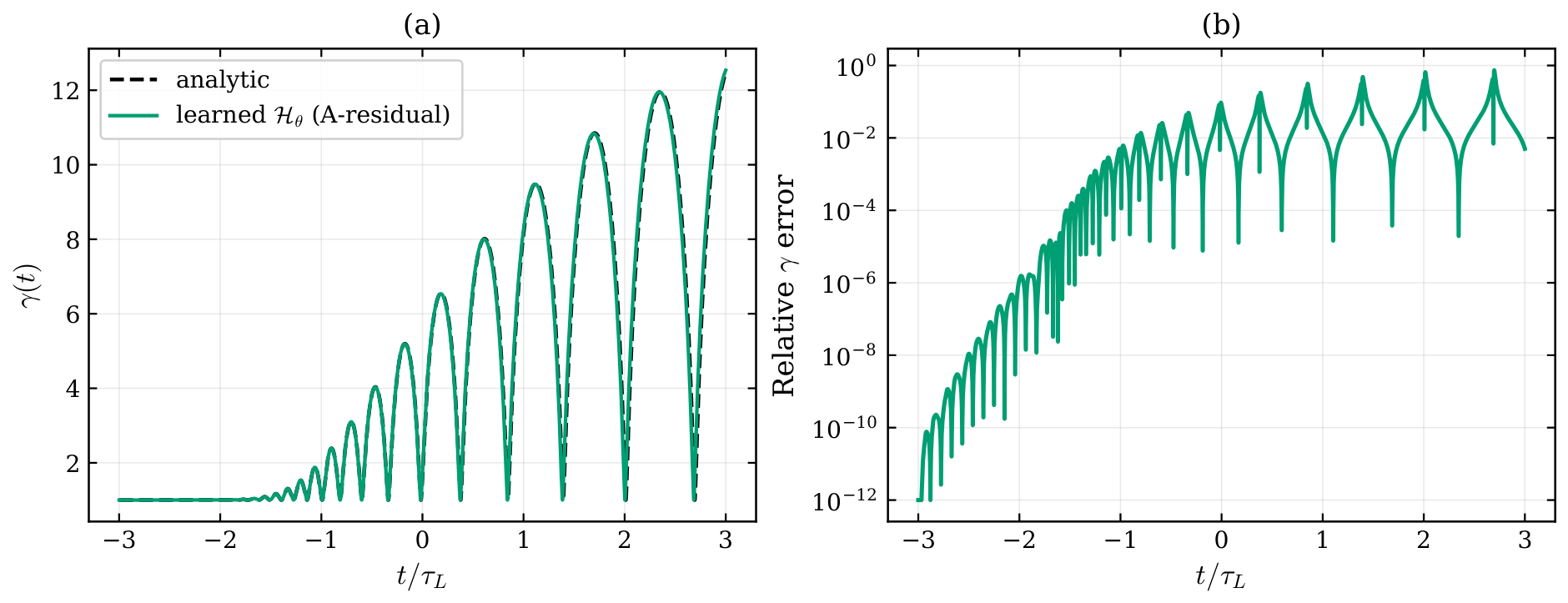
However, a further, more demanding obstacle remains, and we have isolated its origin. The laser-driven quiver is a resonantly forced oscillation, so the ∼1% residual error in the learned force accumulates into a carrier-phase slip; the integrated trajectory keeps the right amplitude but loses phase coherence with the exact solution as the interaction proceeds. Crucially, integrating the learned Hamiltonian with the symplectic Stage-2 map gives the same phase drift as a non-symplectic Runge–Kutta integration: the two learned trajectories are indistinguishable from each other, sharing the same peak instantaneous relative error ${max}_t|{\gamma }_{\mathrm{learned}}-{\gamma }_{\mathrm{exact}}|/{\gamma }_{\mathrm{exact}}\approx 12$ (we use this dimensionless quantity throughout as the trajectory-error metric; a value of order unity corresponds to a full carrier-cycle phase slip, so ≈12 signals a multi-cycle slip; the large value reflects the small denominator at the $\gamma$-troughs, where $\gamma \to 1$ while the phase-slipped curve sits near its peak $\gamma \approx 12$, so it is a phase-coherence indicator rather than a $1200\%$ energy error). The drift is therefore not an integration artifact but a direct consequence of the surrogate error—both integrators faithfully follow the slightly incorrect learned Hamiltonian. Faithful integration of this strongly resonant system thus requires the surrogate force to be far more accurate (we estimate ${\epsilon }_{\theta }\lesssim {10}^{-4}$) than the mass-shell fit alone provides. A substantial improvement comes from a light-cone residual formulation: the analytic plane-wave Hamiltonian—a function of the light-cone phase $\eta =z-ct$—supplies the carrier exactly, and the network learns only the slow focusing correction (a residual that is ∼0.6% of $\mathcal{H}$). This supplies the carrier phase from closed-form physics rather than from the network, and roughly halves the surrogate error (${\epsilon }_{\theta }\approx 5\times {10}^{-3}$) while substantially reducing the trajectory error (to ≈7, from the ≈12 of the tube/Fourier surrogate), with the learned trajectory tracking the exact one further into the interaction. It confirms the light-cone idea as the right direction, but does not by itself fully close the gap. To determine whether the residual drift is a deficiency of the integrator or of the surrogate, we also recast the evolution in the light-cone phase: taking $\eta$ as the independent variable and tracking the slowly varying light-front invariants $(P_x,P_y,\gamma -p_z)$—from which $\gamma$ is reconstructed algebraically together with the analytic field $A_x\left(\eta \right)$—so that the carrier phase is carried by the exact independent variable and cannot accumulate. With the analytic Hamiltonian this scheme reproduces the reference trajectory to $0.25\%$, confirming both the derivation and that the formulation is phase-coherent by construction; with the learned Hamiltonian it nonetheless drifts essentially as before. Together with the symplectic-versus-Runge–Kutta comparison above, this isolates the bottleneck unambiguously: no reformulation of the integration—time-domain, symplectic, or light-cone—can compensate for the ∼1% surrogate force error, which the resonant quiver inevitably amplifies.

Acting directly on this diagnosis, we obtain our best result by reformulating what the network represents: instead of the seven-dimensional Hamiltonian (or its residual), we learn the four-dimensional vector potential in light-cone form (the surrogate variant specified in Section 4.4), $A_{\theta }(x,y,z,t)=A_{\mathrm{pw}}\left(\eta \right)+\mathrm{NN}(x,y,z,t)$, and reconstruct the Hamiltonian analytically as ${\mathcal{H}}_{\theta }=c\sqrt{{(\mathbf{P}-\frac{e}{c}{\mathbf{A}}_{\theta })}^2+m^2{c}^2}$. This formulation is lower-dimensional and structurally exact—the mass-shell constraint holds by construction and the Lorentz force is an exact function of the learned $\partial A_{\theta }$, so the network need only fit a smooth four-dimensional scalar. On a single GPU, with a stabilized optimizer (learning-rate warmup, gradient clipping, an upweighted gradient-matching term, residual-based adaptive resampling of the collocation points, and an L-BFGS polish from the best checkpoint), it reaches ${\epsilon }_{\theta }=(3.0\pm 0.1)\times {10}^{-4}$ (root-mean-square over the in-tube test set, mean ± standard deviation over three seeds), at a training cost of about 20 min per seed on a single NVIDIA Tesla T4 GPU—roughly $2\times {10}^4$ Adam iterations followed by a short L-BFGS polish. The learned-Hamiltonian trajectory then tracks the analytic reference phase-coherently over essentially the whole interaction, with only the final field peak marginally out of phase (Figure 12); the maximum relative $\gamma$ error falls to ≈0.9 ($0.87\pm 0.19$ over three seeds—the mean below unity and the worst seed only marginally above, so the learned and analytic trajectories stay within about one carrier cycle), from ≈12 for the tube/Fourier surrogate and ≈7 for the Hamiltonian residual—and this worst-case figure is dominated by the sharp $\gamma$-troughs, where a sub-cycle phase offset produces a large instantaneous relative error even though the envelope is tracked throughout. That lowering the surrogate force error—by changing what the network represents, with the integrator left untouched—is precisely what restores trajectory fidelity is the clearest confirmation of the diagnosis above; we also find that naively enlarging the network and prolonging training does not help and can destabilize the fit—starting from the same $3.4\times {10}^5$-parameter network at its pre-stabilization accuracy (${\epsilon }_{\theta }\approx 1.2\times {10}^{-3}$, before the learning-rate warmup, gradient-clipping, and adaptive-sampling fixes that yield the headline $(3.0\pm 0.1)\times {10}^{-4}$), doubling the parameter count to $7.5\times {10}^5$ degraded the surrogate error to ${\epsilon }_{\theta }\approx 3.5\times {10}^{-2}$, the Adam optimization diverging mid-training and never recovering the earlier minimum (training log in [36])—so the effective levers are the reformulation and a stabilized optimizer, not raw capacity. Quantitatively, for this best surrogate, the accumulated carrier-phase slip of the transverse momentum—the phase difference between the learned and analytic quivers, extracted from the analytic signal—peaks at only ≈0.16 rad ($\sim 9^{\circ }$) over the interaction at $a_0=5$, ${\tau }_L=30{\omega }_0^{-1}$, consistent with the sub-cycle, envelope-tracking behavior of Figure 12.

Table 5. Laser surrogate variants for the on-axis electron of Section 5.2: in-tube root-mean-square error ${\epsilon }_{\theta }$ of the learned object and its gradients, and the resulting peak relative trajectory error ${max}_t|{\gamma }_{\mathrm{learned}}-{\gamma }_{\mathrm{exact}}|/{\gamma }_{\mathrm{exact}}$. This last column is a phase-coherence indicator, not a fractional energy error: a value of order unity corresponds to a full carrier-cycle phase slip, and the large entries (≈12, ≈7) arise only because the denominator $\gamma \to 1$ at the troughs, where a sub-cycle phase offset inflates the instantaneous ratio (for the best surrogate the accumulated carrier-phase slip is only ≈0.16 rad, ∼$9^{\circ }$). Lowering the surrogate force error—by changing what the network represents, with the integrator left untouched—is what restores trajectory fidelity. All variants use the same $6\times 256$ (∼$3.4\times {10}^5$-parameter) fully-connected network and the same optimization budget (Adam followed by an L-BFGS polish), differing only in the represented object, the input features, and the collocation sampling; the plain-tanh failure (row 1) is therefore an architectural spectral-bias result, not an under-training artifact.

Surrogate Variant	${\mathit{\epsilon }}_{\mathit{\theta }}$ (RMS)	Peak Rel. $\mathit{\gamma }$ Error
Plain tanh, full phase-space box	≈0.8	fails ($\gamma$ stalls $\approx 5$)
Tube sampling + Fourier features	≈$9\times {10}^{-3}$	≈12
Light-cone Hamiltonian residual	≈$5\times {10}^{-3}$	≈7
Vector-potential (A-residual), stabilized	$(3.0\pm 0.1)\times {10}^{-4}$	$0.87\pm 0.19$

summarizes the surrogate variants and the corresponding errors.

Finally, driving this best surrogate through the actual Stage-2 Tao symplectic map—rather than the Runge–Kutta integration used to evaluate it—changes the trajectory by at most $6\times {10}^{-4}$ in $\gamma$, three orders of magnitude below the surrogate-limited error: the complete two-stage SP-PINN pipeline thus reproduces the single-integrator result, confirming directly that the residual error lies entirely in the learned surrogate and not in the geometric integrator. Reaching full quantitative reliability (${\epsilon }_{\theta }\lesssim {10}^{-4}$, now within about a factor of three), for which this vector-potential light-cone formulation is the most promising route, is therefore the single remaining prerequisite for the learned pipeline in the laser regime, and the principal direction of future work.

Second, the surrogate is trained on a bounded phase-space domain; outside it, neural-network extrapolation is uncontrolled, and the Poincaré-invariant diagnostic $\delta I_1\left(t\right)$ can serve as an online detector of such excursions.

Third, the method carries hyperparameter sensitivity: the constraint weight ${\lambda }_1$, network size, learning-rate schedule, and collocation distribution all affect ${\epsilon }_{\theta }$. A distinct, integrator-level sensitivity is the binding constant $\Omega$ of the extended-phase-space map: the bounded error floor depends non-monotonically on $\Omega$ and develops sharp parametric (Floquet) resonances at $2\Omega \Delta t=k\pi$, i.e., along the comb $\Omega \approx k\pi /(2\Delta t)$ (near $\Omega \approx 20$ and $\Omega \approx 50$ here)—derived and numerically verified in Appendix A.2 (Figure A2b)—where the error degrades severely, so $\Omega$ must be placed between bands; this delicacy is a genuine practical limitation of the explicit construction and motivates an adaptive or resonance-avoiding choice of $\Omega$ for production use. The residual-based adaptive collocation refinement [52] adopted for the laser surrogate above is precisely what brought the trajectory error below unity, and a principled automated loss weighting [51] is a natural further step for production use. The supporting numerical studies—a multi-seed assessment of ${\epsilon }_{\theta }$ (Section 5.5), the realized second-order convergence of the Stage-2 map, and the dependence of the bounded error floor on the binding constant $\Omega$ (Appendix A.2)—confirm the robustness of the single-trajectory results reported in the main text.

6.4. Symmetry of the Loss and Geometric Preservation

A conceptual thread directly relevant to this journal connects the symmetry of the training objective to the geometric properties of the resulting integrator. The constraint term is built from the Lorentz scalar $p^{\mu }{p}_{\mu }-m^2{c}^2$ and the residual term from the covariant canonical equations. We are careful here not to overstate the symmetry: the constraint residual ${({\mathcal{H}}_{\theta }-m{c}^2\gamma )}^2$ is evaluated in the laboratory frame and is therefore not manifestly covariant term by term; what is Lorentz-invariant is its target—the mass-shell scalar. Minimizing this lab-frame residual thus enforces a Lorentz-invariant constraint and biases the surrogate toward the covariant mass hyperboloid, rather than making the loss covariant by construction in the strict sense. (A manifestly covariant form would write the residual directly as ${(p^{\mu }{p}_{\mu }-m^2{c}^2)}^2$; the two coincide on shell, and adopting the covariant form explicitly is a natural refinement.) Enforcing a Lorentz-covariant objective biases the network toward a Lorentz-covariant surrogate, yielding a hierarchical chain: Lorentz symmetry of the loss⇒covariant surrogate Hamiltonian⇒mass-shell conservation⇒ Lorentz-group orbit preservation under the symplectic map. In classical symplectic integration, the geometric structure is guaranteed by the algorithm alone; in SP-PINN the physical symmetry of the system is encoded in the loss and transferred, through the trained network, into the geometric structure of the integrator. This symmetry-first viewpoint connects to a growing body of work on symmetry- and conservation-aware learning—symplectic and Lie-group–equivariant models that preserve Noether invariants [55,56], including Lorentz-equivariant architectures for relativistic, high-energy data [57].

6.5. Prospects

Natural extensions include radiation reaction via the Landau–Lifshitz force, which breaks Hamiltonian structure and could be accommodated by a conformal symplectic Stage 2 with an auxiliary dissipation network [58]—or, complementarily, by recasting the non-conservative dynamics in a generalized multi-symplectic form, an approach developed for damped and non-conservative Hamiltonian systems in continuum mechanics [41,59]; application to accelerated (Rindler) frames building on the hyperbolic formalism of [31]; and implementation as a drop-in Boris-pusher replacement in open-source PIC codes, with the Poincaré-invariant diagnostic acting as a self-monitoring symplecticity guard. For such PIC deployment, the chief practical concern is cost at scale: a production run advances ${10}^6$–${10}^9$ particles for ${10}^4$–${10}^6$ steps, so the 7–$20\times$ per-particle overhead of evaluating $\nabla {\mathcal{H}}_{\theta }$ by automatic differentiation at every step (Section 5.6) is the binding constraint, even though it is an $N_p$-independent constant factor that batches efficiently on the GPU (Section 5.6, where throughput already saturates at $2\times {10}^7$ symplectic particle-steps per second for $N_p\gtrsim {10}^5$). The most promising mitigation—which we leave to future work—is to replace the per-step automatic differentiation by learning, once and offline, a Poincaré (one-step) map${\Phi }_{\Delta t}:{(\mathbf{r},\mathbf{P})}_n\mapsto {(\mathbf{r},\mathbf{P})}_{n+1}$ that is symplectic by parametrization—e.g., a SympNet [21] or a generating-function network—so that the online push is a single forward evaluation with no gradient of ${\mathcal{H}}_{\theta }$ at all, collapsing the Yoshida composition’s several autodifferentiations per step into one network call and removing the dominant cost while retaining the symplectic structure. A complementary route is to use the network as a structure-preserving surrogate for the field on the PIC grid rather than for the per-particle force [60]. The ensemble-level structure-preservation result of Section 5.9—the complete learned pipeline reproducing the analytic bunch evolution to better than one percent on $N_p=2500$ electrons—is an encouraging first step toward such collective use, and the Poincaré-loop diagnostic of Section 5.7 provides a built-in, per-step symplecticity guard for it; extending it from this cold, near-axis bunch to a realistic warm-emittance bunch—by training the surrogate on a correspondingly wider tube and quantifying the ${\epsilon }_{\theta }$–tube-width trade-off—is a concrete next step that we, again, regard as companion work rather than a present deliverable. The preservation of the Poincaré–Cartan invariant at the single-particle level is expected to improve the long-term fidelity of collective laser–plasma simulations [1,2].

Finally, the present results single out two quantitative questions for dedicated forthcoming work: what sets the surrogate-accuracy floor ${\epsilon }_{\theta }$, and by what law a small surrogate force error is amplified into the trajectory error of the resonantly driven quiver (Section 6). Preliminary analysis is encouraging on both. The floor appears composite—sampling- and optimization-limited rather than capacity-limited (consistent with the architecture sweep of Appendix A.5) and admitting a Monte-Carlo quadrature upper bound—so that closing it is a matter of sampling and conditioning, not of network expressivity. The amplification, in turn, is governed not by a pessimistic Grönwall exponential but, in the regular (non-chaotic) regime, by a resonant-averaging law linear in time with a relativistic leverage $\sim a_0^2{N}_{\mathrm{cyc}}$ (with $N_{\mathrm{cyc}}$ the number of carrier cycles of interaction)—a structure-dependent “error-amplification operator” that is a property of the dynamics rather than of the particular surrogate, and is therefore expected to recur for other learned-Hamiltonian and reduced-order surrogates. Together these give the operational design requirement ${\epsilon }_{\theta }\lesssim {\delta }_{\mathrm{target}}/\left(C{a}_0^2{N}_{\mathrm{cyc}}\right)$ for a prescribed trajectory accuracy ${\delta }_{\mathrm{target}}$, reframing the surrogate-accuracy bottleneck from “why does the network not train” to “what accuracy budget a given laser regime demands”—the subject of a companion study.

7. Conclusions

We have proposed and tested SP-PINN, a two-stage symmetry-preserving framework for the relativistic equations of motion of a charged particle in 3+1-dimensional electromagnetic fields. An unsupervised physics-informed neural network learns a Lorentz-covariant surrogate Hamiltonian from a mass-shell-constrained loss, and an explicit symplectic map—built on Tao’s extended phase space and therefore applicable to the non-separable relativistic Hamiltonian—advances it while preserving the symplectic structure by construction. We emphasize at the outset that the integrator itself is not learned: to isolate its geometric properties, every benchmark figure advances the analytic relativistic Hamiltonian through Stage 2, while the learned Stage-1 surrogate—the present accuracy bottleneck, not yet competitive with conventional pushers in the static cases—is assessed separately. On a uniform magnetic field, the method exhibits the bounded-versus-secular error contrast: RK4 drifts secularly in the Lorentz factor and Larmor radius, the Boris pusher conserves them to machine precision as a volume-preserving gyro-integrator, and the symplectic SP-PINN map keeps the error bounded for all time, overtaking RK4 within a few hundred gyrations. On a focused Gaussian laser pulse, the method reproduces the ponderomotive dynamics, the energy spectrum, and the conserved transverse canonical momentum, tracking the high-order reference closely. The Lorentz-invariant mass-shell constraint $p^{\mu }{p}_{\mu }=m^2{c}^2$—whose longitudinal restriction is the integral $\gamma \left(\theta \right)=cosh\theta$ of [31]—is preserved to within the training and time-step tolerances, in agreement with Propositions 1 and 2. We have been explicit that on benign integrable benchmarks, a high-order non-symplectic method is competitive and the Boris pusher is optimal for the magnetic sub-problem; the distinctive value of SP-PINN is the absence of secular drift combined with structure-preserving integration of the general non-separable relativistic Hamiltonian. We demonstrated this on a non-integrable magnetic trap, where—no exact volume-preserving rotation being available—the symplectic map alone keeps the energy error bounded while both RK4 and the Boris pusher drift. For the time-dependent laser surrogate, a vector-potential light-cone reformulation brings the learned-Hamiltonian trajectory into phase coherence with the reference over essentially the whole interaction (${\epsilon }_{\theta }=(3.0\pm 0.1)\times {10}^{-4}$ over three seeds), leaving the final approach to ${\epsilon }_{\theta }\lesssim {10}^{-4}$ as the principal open task. We stress that this light-cone A-residual is a problem-specific, near-axis hybrid ansatz rather than a universal device: it presupposes a single dominant retarded phase $\eta =z-ct$ and an analytic plane-wave carrier, so it is most effective for forward-propagating pulses near the optical axis. Field configurations lacking such a phase—counter-propagating or multi-beam geometries with several light cones, tightly focused or structured fields with strong off-axis and longitudinal components, or static and quasi-static configurations—would require either a multi-phase generalization or a return to the direct Hamiltonian surrogate, and are a natural target for future work. We are equally explicit about cost: the symplectic map is several times more expensive per step than the Boris pusher—a bounded constant factor (roughly $7\times$ versus Boris and $3\times$ versus RK4 on a single CPU, and ≈$14\times$ versus Boris at GPU saturation, where the framework overhead is removed and the true arithmetic ratio is exposed; Section 5.5 and Section 5.6)—so SP-PINN is not a universal replacement for Boris but a structure-preserving option for the non-separable problem and for settings where bounded long-time error is the priority. Planned extensions include radiation reaction through conformal symplectic integration, non-inertial reference frames, and integration into a full particle-in-cell loop.

References

1. Gong, Z.; Cao, S.; Palastro, J.P.; Edwards, M.R. Laser Wakefield Acceleration of Ions with a Transverse Flying Focus. Phys. Rev. Lett. 2024, 133, 265002. [Google Scholar] [CrossRef] [PubMed]
2. Aniculaesei, C.; Ha, T.; Yoffe, S.; Labun, L.; Milton, S.; McCary, E.; Spinks, M.M.; Quevedo, H.J.; Labun, O.Z.; Sain, R.; et al. The Acceleration of a High-Charge Electron Bunch to 10 GeV in a 10-cm Nanoparticle-Assisted Wakefield Accelerator. Matter Radiat. Extrem. 2024, 9, 014001. [Google Scholar] [CrossRef]
3. Boris, J.P. Relativistic Plasma Simulation—Optimization of a Hybrid Code. In Proceedings of the Fourth Conference on Numerical Simulation of Plasmas, Naval Research Laboratory, Washington, DC, USA, 2–3 November 1970; pp. 3–67. [Google Scholar]
4. Vay, J.-L. Simulation of Beams or Plasmas Crossing at Relativistic Velocity. Phys. Plasmas 2008, 15, 056701. [Google Scholar] [CrossRef]
5. Higuera, A.V.; Cary, J.R. Structure-Preserving Second-Order Integration of Relativistic Charged Particle Trajectories in Electromagnetic Fields. Phys. Plasmas 2017, 24, 052104. [Google Scholar] [CrossRef]
6. Qin, H.; Zhang, S.; Xiao, J.; Liu, J.; Sun, Y.; Tang, W.M. Why Is Boris Algorithm So Good? Phys. Plasmas 2013, 20, 084503. [Google Scholar] [CrossRef]
7. Zenitani, S.; Umeda, T. On the Boris Solver in Particle-in-Cell Simulation. Phys. Plasmas 2018, 25, 112110. [Google Scholar] [CrossRef]
8. Hairer, E.; Lubich, C. Energy Behaviour of the Boris Method for Charged-Particle Dynamics. BIT Numer. Math. 2018, 58, 969–979. [Google Scholar] [CrossRef]
9. Xiao, J.; Qin, H. Slow Manifolds of Classical Pauli Particle Enable Structure-Preserving Geometric Algorithms for Guiding-Center Dynamics. Comput. Phys. Commun. 2021, 265, 107981. [Google Scholar] [CrossRef]
10. Hairer, E.; Lubich, C.; Wanner, G. Geometric Numerical Integration: Structure-Preserving Algorithms for Ordinary Differential Equations, 2nd ed.; Springer: Berlin/Heidelberg, Germany, 2006. [Google Scholar] [CrossRef]
11. Yoshida, H. Construction of Higher Order Symplectic Integrators. Phys. Lett. A 1990, 150, 262–268. [Google Scholar] [CrossRef]
12. Chin, S.A. Complete Characterization of Fourth-Order Symplectic Integrators with Extended-Linear Coefficients. Phys. Rev. E 2006, 73, 026705. [Google Scholar] [CrossRef] [PubMed]
13. Tao, M. Explicit Symplectic Approximation of Nonseparable Hamiltonians: Algorithm and Long Time Performance. Phys. Rev. E 2016, 94, 043303. [Google Scholar] [CrossRef] [PubMed]
14. He, Y.; Sun, Y.; Liu, J.; Qin, H. Volume-Preserving Algorithms for Charged Particle Dynamics. J. Comput. Phys. 2015, 281, 135–147. [Google Scholar] [CrossRef]
15. Ripperda, B.; Bacchini, F.; Teunissen, J.; Xia, C.; Porth, O.; Sironi, L.; Lapenta, G.; Keppens, R. A Comprehensive Comparison of Relativistic Particle Integrators. Astrophys. J. Suppl. Ser. 2018, 235, 21. [Google Scholar] [CrossRef]
16. Zhang, R.; Liu, T.; Wang, B.; Liu, J.; Tang, Y. Structure-Preserving Algorithm and Its Error Estimate for the Relativistic Charged-Particle Dynamics under the Strong Magnetic Field. J. Sci. Comput. 2024, 100, 70. [Google Scholar] [CrossRef]
17. Zhou, X.-R.; Zhang, L. An Unconditionally-Stable Well-Posed Relativistic Particle Pusher. Comput. Phys. Commun. 2024, 302, 109263. [Google Scholar] [CrossRef]
18. Raissi, M.; Perdikaris, P.; Karniadakis, G.E. Physics-Informed Neural Networks: A Deep Learning Framework for Solving Forward and Inverse Problems Involving Nonlinear Partial Differential Equations. J. Comput. Phys. 2019, 378, 686–707. [Google Scholar] [CrossRef]
19. Karniadakis, G.E.; Kevrekidis, I.G.; Lu, L.; Perdikaris, P.; Wang, S.; Yang, L. Physics-Informed Machine Learning. Nat. Rev. Phys. 2021, 3, 422–440. [Google Scholar] [CrossRef]
20. Greydanus, S.; Dzamba, M.; Yosinski, J. Hamiltonian Neural Networks. Adv. Neural Inf. Process. Syst. 2019, 32, 15353–15363. [Google Scholar]
21. Jin, P.; Zhang, Z.; Zhu, A.; Tang, Y.; Karniadakis, G.E. SympNets: Intrinsic Structure-Preserving Symplectic Networks for Identifying Hamiltonian Systems. Neural Netw. 2020, 132, 166–179. [Google Scholar] [CrossRef] [PubMed]
22. Choudhary, A.; Lindner, J.F.; Holliday, E.G.; Miller, S.T.; Sinha, S.; Ditto, W.L. Physics-Enhanced Neural Networks Learn Order and Chaos. Phys. Rev. E 2020, 101, 062207. [Google Scholar] [CrossRef] [PubMed]
23. Mattheakis, M.; Protopapas, P.; Sondak, D.; Di Giovanni, M.; Kaxiras, E. Physical Symmetries Embedded in Neural Networks. arXiv 2019, arXiv:1904.08991. [Google Scholar] [CrossRef]
24. Toth, P.; Rezende, D.J.; Jaegle, A.; Racanière, S.; Botev, A.; Higgins, I. Hamiltonian Generative Networks. In Proceedings of the 8th International Conference on Learning Representations (ICLR 2020), Addis Ababa, Ethiopia, 26–30 April 2020. [Google Scholar]
25. Canizares, P.; Murari, D.; Schönlieb, C.-B.; Sherry, F.; Shumaylov, Z. Hamiltonian Matching for Symplectic Neural Integrators. arXiv 2024, arXiv:2410.18262. [Google Scholar] [CrossRef]
26. Cheng, X.; Wang, L.; Cao, Y.; Chen, C. Learning Non-Separable Hamiltonian Systems with Pseudo-Symplectic Neural Network. J. Comput. Phys. 2026, 550, 114630. [Google Scholar] [CrossRef]
27. Wu, Y.; Zhang, H.-K.; Duan, H. State–Hamiltonian Neural Networks for Learning Dynamical Systems. Phys. D Nonlinear Phenom. 2025, 483, 134994. [Google Scholar] [CrossRef]
28. Eldred, C.; Gay-Balmaz, F.; Huraka, S.; Putkaradze, V. Lie–Poisson Neural Networks (LPNets): Data-Based Computing of Hamiltonian Systems with Symmetries. Neural Netw. 2024, 173, 106162. [Google Scholar] [CrossRef] [PubMed]
29. Mattheakis, M.; Sondak, D.; Dogra, A.S.; Protopapas, P. Hamiltonian Neural Networks for Solving Equations of Motion. Phys. Rev. E 2022, 105, 065305. [Google Scholar] [CrossRef] [PubMed]
30. Akintsov, N.S.; Nevecheria, A.P.; Kopytov, G.F.; Yang, Y. Lagrangian and Hamiltonian Formalisms for Relativistic Mechanics with Lorentz-Invariant Evolution Parameters in 1+1 Dimensions. Symmetry 2023, 15, 1691. [Google Scholar] [CrossRef]
31. Akintsov, N.S.; Nevecheria, A.P.; Kopytov, G.F.; Yang, Y.; Cao, T. Special Relativity in Terms of Hyperbolic Functions with Coupled Parameters in 3+1 Dimensions. Symmetry 2024, 16, 357. [Google Scholar] [CrossRef]
32. Akintsov, N.S.; Nevecheria, A.P.; Kozhevnikov, V.Y.; Kopytov, G.F.; Cao, T. Integrals of Motion of a Relativistic Particle in 1+1 Dimensions with Coupled Parameters. St. Petersburg Polytech. Univ. J. Phys. Math. 2025, 18, 107–126. [Google Scholar] [CrossRef]
33. Akintsov, N.S.; Nevecheria, A.P.; Yang, Y. Dynamics of a Relativistic Particle in the Field of a Gaussian Laser Pulse in 3+1 Dimensions. Proc. SPIE 2025, 13543, 135430C. [Google Scholar] [CrossRef]
34. Akintsov, N.S.; Nevecheria, A.P.; Kopytov, G.F.; Andreev, S.N.; Yang, Y.; Qin, Q.-H. Invariant Descriptions of Classical Relativistic Particle Motion in 3+1 Dimensions. Mod. Phys. Lett. A 2026, 2650189. [Google Scholar] [CrossRef]
35. Akintsov, N.S.; Nevecheria, A.P.; Andreev, S.N.; Kopytov, G.F. Dynamics of Relativistic Particles in an Ion–Cyclotron Trap in the Presence of an External Ultrashort Laser Pulse. Phys. Plasmas 2025, 32, 082105. [Google Scholar] [CrossRef]
36. Akintsov, N.S.; Nevecheria, A.P. SP-PINN-RelativisticDynamics: Reference Implementation for Symmetry-Preserving Relativistic Charged-Particle Integration, Version 1.3.0; Zenodo. 2026. Available online: https://github.com/NewArtY/SP-PINN-RelativisticDynamics (accessed on 3 July 2026).
37. Liang, C.; Wen, X.; Zhu, Z.; Shen, L.; Wang, Y. SPINI: A Structure-Preserving Neural Integrator for Hamiltonian Dynamics and Parametric Perturbation. Sci. Rep. 2025, 15, 43842. [Google Scholar] [CrossRef] [PubMed]
38. Drimalas, E.G.; Fraschetti, F.; Huang, C.; Tang, Q. Symplectic Neural Network and Its Application to Charged Particle Dynamics in Electromagnetic Fields. Phys. Plasmas 2025, 32, 103901. [Google Scholar] [CrossRef]
39. Jagtap, A.D.; Kharazmi, E.; Karniadakis, G.E. Conservative Physics-Informed Neural Networks on Discrete Domains for Conservation Laws: Applications to Forward and Inverse Problems. Comput. Methods Appl. Mech. Eng. 2020, 365, 113028. [Google Scholar] [CrossRef]
40. Yan, X.; Hu, W.; Han, Z.; Hou, H. Multi-Symplectic Physics-Informed Neural Network for Nonlinear Infinite-Dimensional Hamilton System. Phys. Lett. A 2026, 583, 131616. [Google Scholar] [CrossRef]
41. Yan, X.; Hu, W.; Han, Z. Generalized Multi-Symplectic PINN Method and Its Application in Quantum Tunneling Simulations. Phys. Rev. E 2026, 113, 035308. [Google Scholar] [CrossRef] [PubMed]
42. Landau, L.D.; Lifshitz, E.M. The Classical Theory of Fields, 4th ed.; Course of Theoretical Physics, Volume 2; Pergamon Press: Oxford, UK, 1975. [Google Scholar]
43. Goldstein, H.; Poole, C.P.; Safko, J.L. Classical Mechanics, 3rd ed.; Addison-Wesley: San Francisco, CA, USA, 2001. [Google Scholar]
44. Jackson, J.D. Classical Electrodynamics, 3rd ed.; Wiley: New York, NY, USA, 1999. [Google Scholar]
45. Quesnel, B.; Mora, P. Theory and Simulation of the Interaction of Ultraintense Laser Pulses with Electrons in Vacuum. Phys. Rev. E 1998, 58, 3719–3732. [Google Scholar] [CrossRef]
46. Arnold, V.I. Mathematical Methods of Classical Mechanics, 2nd ed.; Springer: New York, NY, USA, 1989. [Google Scholar] [CrossRef]
47. Abraham, R.; Marsden, J.E. Foundations of Mechanics, 2nd ed.; AMS Chelsea Publishing: Providence, RI, USA, 2008. [Google Scholar] [CrossRef]
48. Frankel, T. The Geometry of Physics: An Introduction, 3rd ed.; Cambridge University Press: Cambridge, UK, 2011. [Google Scholar] [CrossRef]
49. Burby, J.W.; Tang, Q.; Maulik, R. Fast Neural Poincaré Maps for Toroidal Magnetic Fields. Plasma Phys. Control. Fusion 2021, 63, 024001. [Google Scholar] [CrossRef]
50. Fitzpatrick, R. Plasma Physics: An Introduction; Chapter 2 (Charged Particle Motion), Section “Poincaré Invariants”; CRC Press: Boca Raton, FL, USA, 2014; Available online: https://farside.ph.utexas.edu/teaching/plasma/Plasma/node20.html (accessed on 27 July 2026).
51. Wang, S.; Teng, Y.; Perdikaris, P. Understanding and Mitigating Gradient Flow Pathologies in Physics-Informed Neural Networks. SIAM J. Sci. Comput. 2021, 43, A3055–A3081. [Google Scholar] [CrossRef]
52. Wu, C.; Zhu, M.; Tan, Q.; Kartha, Y.; Lu, L. A Comprehensive Study of Non-Adaptive and Residual-Based Adaptive Sampling for Physics-Informed Neural Networks. Comput. Methods Appl. Mech. Eng. 2023, 403, 115671. [Google Scholar] [CrossRef]
53. Kaltsas, D.A. Constrained Hamiltonian Systems and Physics-Informed Neural Networks: Hamilton–Dirac Neural Networks. Phys. Rev. E 2025, 111, 025301. [Google Scholar] [CrossRef] [PubMed]
54. Chu, H.; Miyatake, Y.; Cui, W.; Wei, S.; Furihata, D. Structure-Preserving Physics-Informed Neural Networks with Energy or Lyapunov Structure. In Proceedings of the Thirty-Third International Joint Conference on Artificial Intelligence (IJCAI-24), Jeju, Republic of Korea, 3–9 August 2024; pp. 3872–3880. Available online: https://www.ijcai.org/proceedings/2024/428 (accessed on 27 July 2026).
55. Vaquero, M.; Cortés, J.; Martín de Diego, D. Symmetry Preservation in Hamiltonian Systems: Simulation and Learning. J. Nonlinear Sci. 2024, 34, 115. [Google Scholar] [CrossRef]
56. van der Ouderaa, T.F.A.; van der Wilk, M.; de Haan, P. Noether’s Razor: Learning Conserved Quantities. In Proceedings of the 38th Conference on Neural Information Processing Systems (NeurIPS 2024), Vancouver, BC, Canada, 10–15 December 2024; Advances in Neural Information Processing Systems 37. pp. 135943–135965. [Google Scholar] [CrossRef]
57. Spinner, J.; Bresó, V.; de Haan, P.; Plehn, T.; Thaler, J.; Brehmer, J. Lorentz-Equivariant Geometric Algebra Transformers for High-Energy Physics. In Proceedings of the 38th Conference on Neural Information Processing Systems (NeurIPS 2024), Vancouver, BC, Canada, 10–15 December 2024; Advances in Neural Information Processing Systems. 37, pp. 22178–22205. [Google Scholar] [CrossRef]
58. Zhou, G.; Wang, W.-M.; Li, Y.-T. Solution to the Landau–Lifshitz Equation in Laser and Electrostatic Fields. Phys. Lett. A 2025, 550, 130588. [Google Scholar] [CrossRef]
59. Han, Z.; Hu, W.; Yan, X.; Xiao, C.; Zhang, C.; Deng, Z. Debonding Mechanism Analysis of Ice-Rock Interface Using Frequency Domain Generalized Multi-Symplectic Method. Appl. Math. Model. 2027, 161, 117127. [Google Scholar] [CrossRef]
60. Rettberg, J.; Kneifl, J.; Herb, J.; Buchfink, P.; Fehr, J.; Haasdonk, B. Data-Driven Identification of Latent Port-Hamiltonian Systems. Comput. Sci. Eng. 2025, 2, 4. [Google Scholar] [CrossRef]
Figure 1. Schematic overview of the SP-PINN two-stage architecture. Stage 1 (offline, left): an unsupervised physics-informed neural network H θ ( r , P , t ) is trained on collocation points using the composite loss L total = L eqs + λ 1 L constraint + λ 2 L bc ; no trajectory data are required. Stage 2 (online, right): the frozen surrogate Hamiltonian is embedded in an explicit symplectic map, generating an exactly symplectic discrete flow Φ Δ t ( 4 ) through automatic differentiation. The dashed boundary separates the one-time training phase from the repeated integration phase.
Symmetry 18 01303 g001
Figure 3. Relativistic electron in a focused Gaussian laser pulse ( a 0 = 5 , w 0 = 5 λ 0 , τ L = 30 ω 0 1 ). (a) Longitudinal coordinate z ( t ) and (b) Lorentz factor γ ( t ) for RK4, Boris, SP-PINN (the analytic- H Stage-2 map, as throughout Section 5), and the DOP853 (RK8) reference (black dashed); all four curves overlap. (c) Relative energy error Δ E / E 0 in the later part of the interaction ( t > τ L ). All schemes capture the forward ponderomotive acceleration over this moderate interaction window—the electron co-moves with the pulse and remains in-field, γ oscillating between ≈1 at the carrier troughs and ≈12 at the peaks; RK4 attains the smallest absolute error, Boris the largest, and SP-PINN lies in between, all well below the percent level.
Symmetry 18 01303 g003
Figure 4. (a) Final kinetic-energy spectrum d N / d γ of 256 electrons with uniformly distributed initial transverse positions after the Gaussian pulse has passed, for RK4, Boris, SP-PINN (analytic- H Stage-2 map), and a fine-step reference. (b) Numerical violation of the transverse canonical momentum P x = p x + ( e / c ) A x , the Noether invariant of the transverse translational symmetry, for an on-axis electron, measured as the deviation from the DOP853 reference. The Boris pusher shows by far the largest symmetry violation (∼ 4 × 10 2 ); RK4 is the most accurate here (∼ 10 8 ) and the SP-PINN map is intermediate (∼ 3 × 10 5 )—its bounded binding floor rather than machine precision, reflecting the frozen-in-time (non-strictly-symplectic) laser map of Section 5.2.
Symmetry 18 01303 g004
Figure 5. Non-integrable autonomous system: a charged particle in B = B 0 z ^ plus the anharmonic well φ = 1 2 k ( x 2 + y 2 ) + ϵ x 2 y 2 ( B 0 = k = 1 , ϵ = 0.3 ). (a) A representative chaotic orbit in the ( x , y ) plane (gray; computed with the SP-PINN map, shown to illustrate the dynamics rather than as a method comparison). (b) Relative energy error | H ( t ) H 0 | / | H 0 | over 3 × 10 5 steps ( Δ t = 0.05 , Ω = 10 ): RK4 (blue, solid) drifts secularly, the Boris pusher (orange, dashed) shows the largest error for this nonlinear static field, and the symplectic SP-PINN map (green, dotted) keeps the error bounded.
Symmetry 18 01303 g005
Figure 6. Rotational and gauge symmetry (Section 5.4). (a) Relative drift of the canonical angular momentum L z = x P y y P x —the Noether invariant of the rotational symmetry of B = B 0 z ^ plus the axisymmetric well φ ( ρ ) = 1 2 k ρ 2 + β ρ 4 —for RK4, Boris, Higuera–Cary, and the symplectic SP-PINN map. The volume-preserving but non-symplectic Boris and Higuera–Cary pushers drift most (∼ 10 3 , secularly); the symplectic map keeps L z bounded (≲ 5 × 10 6 , flat), mirroring the transverse-momentum result of Figure 4b. (b) Gauge invariance of the canonical Stage-2 map: the physical trajectory computed in the symmetric and Landau gauges agrees to ∼ 10 5 in both position and kinetic momentum, i.e., to the integrator’s truncation level.
Symmetry 18 01303 g006
Figure 7. Total wall-clock time per integration step for Boris, RK4, and the SP-PINN symplectic map (analytic- H Stage-2 map) as a function of the number of particles N p integrated in parallel (batched NumPy, single CPU), on the magnetic-field problem. The total time grows sublinearly with N p , so the per-particle cost decreases under batching; the SP-PINN cost ratio nonetheless remains ≈ 7 × versus Boris (≈ 3 × versus RK4) at all batch sizes. The one-time offline Stage-1 training cost is not included.
Symmetry 18 01303 g007
Figure 8. GPU throughput (particle-steps per second, double precision, NVIDIA Tesla P100) of Boris, RK4, and the SP-PINN symplectic (Tao) map versus ensemble size N p on the uniform-field problem. Throughput saturates above N p 10 5 ; the SP-PINN/Boris overhead is a bounded, N p -independent constant factor (≈ 14 × ), not a scaling penalty.
Symmetry 18 01303 g008
Figure 9. Geometric-invariant conservation, comparator set {Boris, Higuera–Cary, RK4, Tao}. Top: relative drift δ I 1 ( t ) of the first Poincaré–Cartan loop invariant ( M = 256 ) for (a) the uniform field, (b) the focused laser, (c) the chaotic magnetic trap. The symplectic Tao map keeps δ I 1 bounded; Boris and Higuera–Cary, volume preserving but not symplectic, drift at O ( Δ t ) . Bottom: relative energy drift δ H ( t ) for the two autonomous cases. (d) Uniform field: Boris and Higuera–Cary conserve the energy to machine precision ( 10 15 ), RK4 drifts secularly, and the Tao map oscillates within a bounded band at 10 5 set by its binding constant. (e) Chaotic magnetic trap: the Tao map stays bounded at 3 × 10 5 , whereas Boris and Higuera–Cary drift secularly to 10 2 , about 2.5 orders larger, and RK4—also secular, but high order—sits between them. The laser case has no panel here because its Hamiltonian is explicitly time dependent, so the energy is not a constant of motion.
Symmetry 18 01303 g009
Figure 10. A single A-residual surrogate trained over the pulse-duration family τ L [ 20 , 40 ] ω 0 1 (green shaded band). The blue marker line is the in-tube root-mean-square error ε θ ( τ L ) of that one trained network, evaluated at seven pulse durations; the two outermost points ( τ L = 15 and τ L = 45 ) lie outside the shaded band and are therefore extrapolation. The error stays at ( 3 7 ) × 10 4 across the trained band—matching the single-pulse value at τ L = 30 —and degrades gracefully under extrapolation.
Symmetry 18 01303 g010
Figure 11. Complete learned pipeline (learned A θ + Stage-2 Tao map) on a cold bunch of N p = 2500 electrons in the focused pulse, against the analytic- H Tao reference and Boris/RK4. (a) Transverse emittance, (b) mean Lorentz factor, (c) relative energy spread versus t / τ L . All curves overlap; the learned pipeline matches the analytic bunch to < 1 % in every observable.
Symmetry 18 01303 g011
Figure 12. The learned Stage-1 surrogate in action—the one figure of this paper that uses the trained network rather than the analytic Hamiltonian. The on-axis electron of Section 5.2 is integrated with the learned Hamiltonian H θ = c ( P e c A θ ) 2 + m 2 c 2 built from the A-residual vector-potential surrogate A θ = A pw ( η ) + NN ( x , y , z , t ) ( ε θ = ( 3.0 ± 0.1 ) × 10 4 over three seeds). (a) Lorentz factor γ ( t ) of the learned trajectory (green) against the analytic reference (black dashed): the two overlap over essentially the entire interaction, separating only at the final field peak. (b) Relative γ error: the envelope is tracked throughout, and the worst-case value (≈0.7 for the seed shown; 0.87 ± 0.19 over three seeds) occurs at the sharp γ -troughs, where a sub-cycle phase offset yields a large instantaneous relative error. This demonstrates the learned pipeline; closing the residual end-of-pulse slip requires ε θ 10 4 (Section 6).
Symmetry 18 01303 g012