The Contrastive Sombor Index: Structural Properties and Applications to Monogenic Semigroup Graphs

Abstract

The Sombor index has recently become a central tool among degree-based graph invariants; however, it does not explicitly isolate degree imbalance along edges. In this work, we introduce the degree-based Contrastive Sombor Index (CSO), which combines endpoint-degree magnitude with local degree imbalance. For a finite simple graph $G=(V,E)$, the index is defined by $\mathrm{CSO}\left(G\right)={\displaystyle \sum _{uv\in E\left(G\right)}}\left(\sqrt{d{\left(u\right)}^2+d{\left(v\right)}^2}-\sqrt{2}\min \{d\left(u\right),d\left(v\right)\}\right).$ Unlike the Sombor index, which primarily reflects the magnitude of the endpoint degrees, the CSO contribution vanishes when the endpoint degrees are equal and responds to degree imbalance while retaining degree-scale information. In particular, it can distinguish certain graphs having the same total edgewise irregularity but different endpoint-degree distributions. In this work, we first show that $CSO\left(G\right)\ge 0$ and prove that $CSO\left(G\right)=0$ if and only if each connected component of G is regular. We also establish general lower and upper bounds for CSO. In addition, we obtain a relation connecting the CSO index with the first Zagreb index and the edgewise degree differences. We also discuss extremal aspects of the index. As an application, we derive an explicit summation formula for CSO on monogenic semigroup graphs. From our computations on $\Gamma \left(S_M\right)$, it follows that the asymptotic growth order of the index satisfies $CSO(\Gamma \left(S_M\right))=\Theta \left(n^3\right).$ These results show that the CSO index combines degree-magnitude information with sensitivity to unequal endpoint degrees and provides an additional perspective on degree heterogeneity in graphs.

1. Introduction

Let G be a simple graph with vertex set $V\left(G\right)$ and edge set $E\left(G\right)$. For a vertex $v\in V\left(G\right)$, we denote its degree by $d\left(v\right)$ and we represent by $uv$ the edge connecting the vertices u and v. For additional background on graph theoretic notions, see [1].

We consider a finite multiplicative monogenic semigroup with zero of the form

$$S_M=\{0,x,x^2,x^3,\dots ,x^n\},$$

as introduced in [2]. The graph $\Gamma \left(S_M\right)$ is defined by retaining the vertex set and imposing a specific adjacency rule. The vertex set of $\Gamma \left(S_M\right)$ consists of all nonzero elements of $S_M$.

Two distinct vertices $x^i$ and $x^j$ in $\Gamma \left(S_M\right)$, where $1\le i,j\le n$, are adjacent precisely when $i+j>n$. Further background on monogenic semigroup graphs can be found in [2,3,4].

Monogenic semigroup graphs arise as a natural extension of the theory of zero-divisor graphs [2]. The study of zero-divisor graphs in commutative rings was initiated by Beck [5] and subsequently developed in its modern form by Anderson and Livingston [6], with further developments appearing in [7]. Similar ideas were later extended to commutative and non-commutative semigroups [8,9].

Topological indices have been studied extensively in chemical graph theory and provide numerical descriptions of molecular and graph structures [10,11]. Among the degree-based topological indices, the Sombor index, introduced by Furtula and Gutman [12], has attracted considerable attention in both chemical graph theory and purely mathematical research [13,14]. For a graph G, the Sombor index is defined by

$$SO\left(G\right)=\sum _{uv\in E\left(G\right)}\sqrt{d{\left(u\right)}^2+d{\left(v\right)}^2},$$

where the summation extends over all edges of G, and $d\left(u\right)$ and $d\left(v\right)$ denote the degrees of the corresponding adjacent vertices. The Sombor index has also been investigated in algebraic settings, including graphs associated with monogenic semigroups [3,4].

The Sombor index measures the magnitude of the degrees at the endpoints of an edge. However, it does not explicitly isolate the degree difference between adjacent vertices. A classical measure of local degree imbalance is the total edgewise irregularity

$$\mathrm{irr}\left(G\right)=\sum _{uv\in E\left(G\right)}|d\left(u\right)-d\left(v\right)|,$$

which records the absolute degree differences along the edges [15]. Although this quantity captures degree imbalance, it does not account for the scale of the endpoint degrees.

Motivated by these complementary features, we introduce the Contrastive Sombor Index (CSO). For a finite simple graph $G=(V,E)$, it is defined by

$$CSO\left(G\right)=\sum _{uv\in E\left(G\right)}\left(\sqrt{d{\left(u\right)}^2+d{\left(v\right)}^2}-\sqrt{2}\min \{d\left(u\right),d\left(v\right)\}\right).$$

The subtraction of the minimum-degree term makes an edge contribution vanish when its endpoints have equal degrees, while the square-root term retains information about the magnitude of the endpoint degrees. Thus, the CSO index combines local degree imbalance with degree-scale information.

The CSO index is closely related to existing degree-based invariants. Indeed, as proved in Theorem 3, it satisfies

$$CSO\left(G\right)=SO\left(G\right)-{\displaystyle \frac{\sqrt{2}}{2}}{M}_1\left(G\right)+{\displaystyle \frac{\sqrt{2}}{2}}\sum _{uv\in E\left(G\right)}|d\left(u\right)-d\left(v\right)|,$$

where

$$M_1\left(G\right)=\sum _{v\in V\left(G\right)}d{\left(v\right)}^2$$

is the first Zagreb index. Equivalently, using

$$\mathrm{irr}\left(G\right)=\sum _{uv\in E\left(G\right)}|d\left(u\right)-d\left(v\right)|,$$

the decomposition may be written as

$$CSO\left(G\right)=SO\left(G\right)-{\displaystyle \frac{\sqrt{2}}{2}}{M}_1\left(G\right)+{\displaystyle \frac{\sqrt{2}}{2}}\mathrm{irr}\left(G\right).$$

Therefore, CSO is not independent of the Sombor index, the first Zagreb index, and the total edgewise degree irregularity. Its contribution lies in combining degree magnitude, degree intensity, and local degree imbalance within a single edge-based expression.

The following example shows that two graphs may have the same total edgewise irregularity $\mathrm{irr}\left(G\right)$ but different CSO values, because CSO also retains information about the scale and distribution of the endpoint degrees.

Example 1.

Consider the star graph $K_{1,3}$. Each of its three edges has degree pair $(3,1)$, and therefore

$$\mathrm{irr}\left(K_{1,3}\right)=3|3-1|=6.$$

Its Contrastive Sombor Index is

$$CSO\left(K_{1,3}\right)=3\left(\sqrt{3^2+1^2}-\sqrt{2}\right)=3\left(\sqrt{10}-\sqrt{2}\right)\approx 5.2442.$$

Now consider the complete bipartite graph $K_{2,3}$. Each of its six edges has degree pair $(3,2)$, and hence

$$\mathrm{irr}\left(K_{2,3}\right)=6|3-2|=6.$$

On the other hand,

$$CSO\left(K_{2,3}\right)=6\left(\sqrt{3^2+2^2}-2\sqrt{2}\right)=6\left(\sqrt{13}-2\sqrt{2}\right)\approx 4.6627.$$

Consequently,

$$\mathrm{irr}\left(K_{1,3}\right)=\mathrm{irr}\left(K_{2,3}\right),CSO\left(K_{1,3}\right)\ne CSO\left(K_{2,3}\right).$$

Thus, the CSO index can distinguish graphs having the same total edgewise degree difference because it also incorporates the scale of the endpoint degrees.

This comparison does not imply that the CSO index is universally superior to existing irregularity indices. Rather, it shows that CSO retains degree-scale information that is not captured by the total edgewise degree difference alone.

The main components of the paper are organized as follows. In Section 2, we introduce the Contrastive Sombor Index and investigate its fundamental structural properties, including its connection with graph regularity and classical degree-based invariants. In Section 3, we establish general lower and upper bounds. Section 4 is devoted to monogenic semigroup graphs, where we develop a neighborhood–block decomposition, derive explicit summation formulas, and determine the asymptotic growth of the index. Section 5 illustrates the explicit formulas through the cases $n=5$ and $n=6$. In Section 6, we analyze individual edge contributions and clarify the dependence of CSO on degree imbalance and endpoint-degree scale. Finally, Section 7 provides a numerical illustration based on the octane-isomer dataset.

2. Definition and Structural Properties of the Contrastive Sombor Index

In this section, we present the definition of the Contrastive Sombor Index (CSO) and investigate its fundamental structural properties; we establish the mathematical framework of the index by examining its relationship with graph regularity and by deriving basic inequalities. We also obtain a decomposition formula connecting CSO with the Sombor and Zagreb indices and determine its explicit value for star graphs.

Definition 1.

Let $G=(V,E)$ be a finite simple graph, not necessarily connected and possibly containing isolated vertices, with degree function $d(·)$. The Contrastive Sombor Index of G is defined by

$$\mathrm{CSO}\left(G\right)=\sum _{uv\in E\left(G\right)}\left(\sqrt{d{\left(u\right)}^2+d{\left(v\right)}^2}-\sqrt{2}\min \{d\left(u\right),d\left(v\right)\}\right).$$

Proposition 1.

For every simple graph G, one has $\mathrm{CSO}\left(G\right)\ge 0$.

Proof. 

For each edge $uv\in E\left(G\right)$, assume without loss of generality that $d\left(u\right)\le d\left(v\right)$. Then,

$$\sqrt{d{\left(u\right)}^2+d{\left(v\right)}^2}\ge \sqrt{d{\left(u\right)}^2+d{\left(u\right)}^2}=\sqrt{2}d\left(u\right)=\sqrt{2}\min \{d\left(u\right),d\left(v\right)\}.$$

Hence, each summand is nonnegative, and summing over all edges gives $\mathrm{CSO}\left(G\right)\ge 0$. □

We now characterize the case when the index attains its minimum value.

Theorem 1 (Rigidity of CSO).

For a simple graph G, the following are equivalent:

1.

$\mathrm{CSO}\left(G\right)=0$;

2.

every edge $uv\in E\left(G\right)$ satisfies $d\left(u\right)=d\left(v\right)$.

In particular, $CSO\left(G\right)=0$ if and only if every connected component of G is regular. Consequently, if G is connected, then $CSO\left(G\right)=0$ if and only if G is regular.

Proof. 

Suppose first that every edge $uv\in E\left(G\right)$ satisfies $d\left(u\right)=d\left(v\right)$. Then, for each edge,

$$\sqrt{d{\left(u\right)}^2+d{\left(v\right)}^2}=\sqrt{2}d\left(u\right)=\sqrt{2}\min \{d\left(u\right),d\left(v\right)\}.$$

Hence, each summand vanishes and $\mathrm{CSO}\left(G\right)=0$.

Conversely, assume $\mathrm{CSO}\left(G\right)=0$. Since each summand is nonnegative, every term must be zero. Thus, for every edge $uv$,

$$\sqrt{d{\left(u\right)}^2+d{\left(v\right)}^2}=\sqrt{2}\min \{d\left(u\right),d\left(v\right)\},$$

which holds if and only if $d\left(u\right)=d\left(v\right)$. Hence, adjacent vertices have equal degrees.

Degree equality propagates along every path. Therefore, all vertices belonging to the same connected component have the same degree, so each connected component containing at least one edge is regular. An isolated vertex forms a 0-regular component. Consequently, $CSO\left(G\right)=0$ if and only if every connected component of G is regular. In particular, if G is connected, then $CSO\left(G\right)=0$ if and only if G is regular. □

As a direct consequence of Theorem 1, we obtain the following result for complete graphs.

Corollary 1.

Let G be the complete graph $K_n$. Then,

$$\mathrm{CSO}\left(K_n\right)=0.$$

Proof. 

Every vertex of $K_n$ has degree $n-1$, so all adjacent vertices have equal degrees. Therefore, $\mathrm{CSO}\left(K_n\right)=0$. □

Corollary 2.

Let $K_{1,n-1}$ be the star graph on $n\ge 2$ vertices. Then,

$$\mathrm{CSO}\left(K_{1,n-1}\right)=(n-1)\left(\sqrt{{(n-1)}^2+1}-\sqrt{2}\right).$$

Proof. 

In $K_{1,n-1}$, the central vertex has degree $n-1$ and each leaf has degree 1. Each edge therefore contributes

$$\sqrt{{(n-1)}^2+1}-\sqrt{2}.$$

Since there are $n-1$ edges, the result follows. □

The star graph not only provides an explicit example, but also represents an extremal structure for the Contrastive Sombor index among trees.

Theorem 2.

Let T be a tree on $n\ge 2$ vertices. Then,

$$\mathrm{CSO}\left(T\right)\le (n-1)\left(\sqrt{{(n-1)}^2+1}-\sqrt{2}\right).$$

Equality holds if and only if

$$T\cong K_{1,n-1}.$$

Consequently, the star graph $K_{1,n-1}$ uniquely maximizes the Contrastive Sombor Index among all trees on n vertices.

Proof. 

Let $uv\in E\left(T\right)$, and set

$$x=\min \left\{d\right(u),d(v\left)\right\},y=\max \left\{d\right(u),d(v\left)\right\}.$$

Since T is a tree on n vertices,

$$1\le x\le y\le n-1.$$

The contribution of the edge $uv$ to $\mathrm{CSO}\left(T\right)$ is

$$\varphi (x,y)=\sqrt{x^2+y^2}-\sqrt{2}x.$$

For fixed x, we have

$${\displaystyle \frac{\partial \varphi }{\partial y}}={\displaystyle \frac{y}{\sqrt{x^2+y^2}}}>0,$$

so $\varphi (x,y)$ is strictly increasing in y. For fixed y,

$${\displaystyle \frac{\partial \varphi }{\partial x}}={\displaystyle \frac{x}{\sqrt{x^2+y^2}}}-\sqrt{2}<0,$$

because

$${\displaystyle \frac{x}{\sqrt{x^2+y^2}}}<1<\sqrt{2}.$$

Thus, $\varphi (x,y)$ is strictly decreasing in x. It follows that

$$\varphi (x,y)\le \varphi (1,n-1)=\sqrt{{(n-1)}^2+1}-\sqrt{2}.$$

Every tree on n vertices has exactly $n-1$ edges. Therefore, summing the preceding pointwise inequality over all edges gives

$$\mathrm{CSO}\left(T\right)\le (n-1)\left(\sqrt{{(n-1)}^2+1}-\sqrt{2}\right).$$

We emphasize that this argument does not assume that the endpoint degrees of different edges can be maximized independently. It establishes a universal upper bound for each edge contribution and then determines when equality can hold simultaneously on all edges.

Suppose that equality holds in the global bound. Since the inequality for each edge is strict unless $x=1$ and $y=n-1$, every edge of T must have endpoint-degree pair

$$(1,n-1).$$

In particular, T contains a vertex c satisfying

$$d\left(c\right)=n-1.$$

By the Handshaking Lemma,

$$\sum _{v\in V\left(T\right)}d\left(v\right)=2\left|E\left(T\right)\right|=2n-2.$$

After subtracting the degree of c, the sum of the degrees of the remaining $n-1$ vertices is

$$\sum _{v\in V\left(T\right)\setminus \left\{c\right\}}d\left(v\right)=(2n-2)-(n-1)=n-1.$$

Because T is connected, each of the remaining $n-1$ vertices has degree at least one. Hence,

$$T\cong K_{1,n-1}.$$

Conversely, every edge of $K_{1,n-1}$ has endpoint-degree pair $(1,n-1)$. Since $K_{1,n-1}$ has $n-1$ edges,

$$\mathrm{CSO}\left(K_{1,n-1}\right)=(n-1)\left(\sqrt{{(n-1)}^2+1}-\sqrt{2}\right).$$

Therefore, equality holds if and only if $T\cong K_{1,n-1}$, completing the proof. □

2.1. Extremal Behavior Beyond Trees

Theorem 2 shows that the star graph $K_{1,n-1}$ uniquely maximizes the Contrastive Sombor Index among all trees on n vertices. It is natural to ask whether this extremal property extends to larger classes of graphs.

However, this is not the case for general graphs. One can construct graphs on n vertices with larger CSO values than the star graph. To provide an explicit example, consider the graph $G^{*}$ on $n=6$ vertices obtained by joining every vertex of the complete graph $K_2$ to every vertex of the edgeless graph ${\overline{K}}_4$. The two vertices of $K_2$ have degree 5, while the four vertices of ${\overline{K}}_4$ have degree 2.

The edge set of $G^{*}$ consists of one edge with endpoint-degree pair $(5,5)$, which contributes zero to the index, and eight edges with endpoint-degree pair $(5,2)$. Consequently,

$$\begin{array}{cc}\hfill \mathrm{CSO}\left(G^{*}\right)& =8\left(\sqrt{5^2+2^2}-2\sqrt{2}\right)\hfill \\ & =8\left(\sqrt{29}-2\sqrt{2}\right)\approx 20.4539.\hfill \end{array}$$

On the other hand, for the star graph $K_{1,5}$ on six vertices, Corollary 2 gives

$$\mathrm{CSO}\left(K_{1,5}\right)=5\left(\sqrt{26}-\sqrt{2}\right)\approx 18.4240.$$

Since

$$\mathrm{CSO}\left(G^{*}\right)>\mathrm{CSO}\left(K_{1,5}\right),$$

this example demonstrates that the restriction to trees is essential. Characterizing the extremal graphs among all graphs of a fixed order remains an open problem.

Proposition 2.

For every simple graph G, the following identity holds:

$$\mathrm{SO}\left(G\right)-\mathrm{CSO}\left(G\right)=\sqrt{2}\sum _{uv\in E\left(G\right)}\min \{d\left(u\right),d\left(v\right)\}.$$

Proof. 

By definition,

$$\mathrm{SO}\left(G\right)=\sum _{uv\in E\left(G\right)}\sqrt{d{\left(u\right)}^2+d{\left(v\right)}^2},$$

and

$$\mathrm{CSO}\left(G\right)=\sum _{uv\in E\left(G\right)}\left(\sqrt{d{\left(u\right)}^2+d{\left(v\right)}^2}-\sqrt{2}\min \{d\left(u\right),d\left(v\right)\}\right).$$

Subtracting the second expression from the first gives

$$\mathrm{SO}\left(G\right)-\mathrm{CSO}\left(G\right)=\sum _{uv\in E\left(G\right)}\sqrt{2}\min \{d\left(u\right),d\left(v\right)\},$$

which proves the claim. □

Theorem 3.

For every simple graph G, the Contrastive Sombor Index satisfies the decomposition formula

$$\mathrm{CSO}\left(G\right)=\mathrm{SO}\left(G\right)-{\displaystyle \frac{\sqrt{2}}{2}}{M}_1\left(G\right)+{\displaystyle \frac{\sqrt{2}}{2}}\sum _{uv\in E\left(G\right)}|d\left(u\right)-d\left(v\right)|,$$

where

$$M_1\left(G\right)=\sum _{v\in V\left(G\right)}d{\left(v\right)}^2$$

is the first Zagreb index.

Proof. 

By Proposition 2, we have

$$\mathrm{SO}\left(G\right)-\mathrm{CSO}\left(G\right)=\sqrt{2}\sum _{uv\in E\left(G\right)}\min \{d\left(u\right),d\left(v\right)\}.$$

Using the identity

$$\min \{a,b\}={\displaystyle \frac{a+b-|a-b|}{2}},$$

we obtain

$$\begin{array}{cc}\hfill \sum _{uv\in E\left(G\right)}\min \{d\left(u\right),d\left(v\right)\}& ={\displaystyle \frac{1}{2}}\sum _{uv\in E\left(G\right)}\left(d\left(u\right)+d\left(v\right)\right)\hfill \\ & -{\displaystyle \frac{1}{2}}\sum _{uv\in E\left(G\right)}|d\left(u\right)-d\left(v\right)|.\hfill \end{array}$$

By double counting the contribution of each vertex degree over the edge set, each vertex v contributes $d\left(v\right)$ once for every incident edge, and hence

$$\sum _{uv\in E\left(G\right)}\left(d\left(u\right)+d\left(v\right)\right)=\sum _{v\in V\left(G\right)}d{\left(v\right)}^2=M_1\left(G\right).$$

Therefore,

$$\sum _{uv\in E\left(G\right)}\min \{d\left(u\right),d\left(v\right)\}={\displaystyle \frac{1}{2}}{M}_1\left(G\right)-{\displaystyle \frac{1}{2}}\sum _{uv\in E\left(G\right)}|d\left(u\right)-d\left(v\right)|.$$

Substituting this expression into the initial identity gives

$$\mathrm{SO}\left(G\right)-\mathrm{CSO}\left(G\right)={\displaystyle \frac{\sqrt{2}}{2}}{M}_1\left(G\right)-{\displaystyle \frac{\sqrt{2}}{2}}\sum _{uv\in E\left(G\right)}|d\left(u\right)-d\left(v\right)|.$$

Rearranging the terms yields

$$\mathrm{CSO}\left(G\right)=\mathrm{SO}\left(G\right)-{\displaystyle \frac{\sqrt{2}}{2}}{M}_1\left(G\right)+{\displaystyle \frac{\sqrt{2}}{2}}\sum _{uv\in E\left(G\right)}|d\left(u\right)-d\left(v\right)|,$$

which completes the proof. □

This decomposition consists of three components: the Sombor term, the Zagreb term, and the total degree difference along the edges. The last component corresponds to the total degree imbalance along the edges.

2.2. A Comparative Illustration

The Sombor index reflects the magnitude of the degrees at the endpoints of edges, but it does not explicitly capture how different these degrees are. To highlight the structural sensitivity of the Contrastive Sombor Index, we consider graphs with different degree distributions.

(1) Cycle $C_4$. The degree sequence is $(2,2,2,2)$, so the graph is regular. We obtain

$$SO\left(C_4\right)=4\sqrt{8},CSO\left(C_4\right)=0.$$

Since all adjacent vertices have equal degrees, no local imbalance occurs.

(2) Path $P_4$. The degree sequence is $(1,2,2,1)$. Direct computation yields

$$SO\left(P_4\right)=2\sqrt{5}+\sqrt{8},CSO\left(P_4\right)=2(\sqrt{5}-\sqrt{2}).$$

Here, the graph exhibits moderate degree imbalance along its edges.

(3) Star $K_{1,3}$. The degree sequence is $(3,1,1,1)$. We obtain

$$SO\left(K_{1,3}\right)=3\sqrt{10},CSO\left(K_{1,3}\right)=3(\sqrt{10}-\sqrt{2}).$$

Each edge connects vertices with highly unequal degrees, producing strong local imbalance.

These examples illustrate that the Sombor and Contrastive Sombor indices respond differently to variations in the endpoint degrees. The CSO index vanishes on regular graphs, whereas edges joining vertices of unequal degrees may make positive contributions. As will be established more precisely in Lemma 2, when the smaller endpoint degree is fixed, the edge contribution increases strictly with the larger endpoint degree. Thus, CSO reflects both local degree imbalance and the scale of the endpoint degrees.

3. Bounds for the Contrastive Sombor Index

In this section, we derive general lower and upper bounds for the Contrastive Sombor Index. Throughout, let $m=\left|E\right(G\left)\right|$ denote the number of edges of G, and let

$$\delta =\underset{v\in V\left(G\right)}{\min }d\left(v\right)$$

be the minimum vertex degree.

Theorem 4.

For every simple graph G with m edges and minimum degree δ,

$$\mathrm{SO}\left(G\right)-\mathrm{CSO}\left(G\right)\ge \sqrt{2}m\delta .$$

Proof. 

By Proposition 2,

$$\mathrm{SO}\left(G\right)-\mathrm{CSO}\left(G\right)=\sqrt{2}\sum _{uv\in E\left(G\right)}\min \{d\left(u\right),d\left(v\right)\}.$$

Since $\delta \le d\left(u\right)$ and $\delta \le d\left(v\right)$ for all vertices,

$$\min \left\{d\right(u),d(v\left)\right\}\ge \delta$$

for every edge $uv$. Hence,

$$\sum _{uv\in E\left(G\right)}\min \{d\left(u\right),d\left(v\right)\}\ge m\delta ,$$

which yields the desired inequality. □

We now relate the Contrastive Sombor index to the total degree difference along edges.

Theorem 5.

For every simple graph G, the Contrastive Sombor index satisfies

$$\mathrm{CSO}\left(G\right)\ge {\displaystyle \frac{1}{\sqrt{2}}}\sum _{uv\in E\left(G\right)}|d\left(u\right)-d\left(v\right)|.$$

Proof. 

For any $a,b\ge 0$, we use the inequality

$$\sqrt{a^2+b^2}\ge {\displaystyle \frac{a+b}{\sqrt{2}}},$$

which follows from ${(a-b)}^2\ge 0$.

We may assume, without loss of generality, that $d\left(u\right)\le d\left(v\right)$. Then, $\min \left\{d\right(u),d(v\left)\right\}=d\left(u\right)$, and thus

$$\sqrt{d{\left(u\right)}^2+d{\left(v\right)}^2}-\sqrt{2}\min \{d\left(u\right),d\left(v\right)\}\ge {\displaystyle \frac{d\left(u\right)+d\left(v\right)}{\sqrt{2}}}-\sqrt{2}d\left(u\right)={\displaystyle \frac{d\left(v\right)-d\left(u\right)}{\sqrt{2}}}={\displaystyle \frac{\left|d\right(u)-d(v\left)\right|}{\sqrt{2}}}.$$

Summing over all edges gives the result. □

Corollary 3.

Equality in Theorem 4 holds if and only if

$$\min \left\{d\right(u),d(v\left)\right\}=\delta \mathit{for} \mathit{every} \mathit{edge} uv\in E\left(G\right).$$

In particular, equality holds when every edge is incident to a vertex of minimum degree.

Proof. 

Equality in Theorem 4 requires

$$\min \left\{d\right(u),d(v\left)\right\}=\delta$$

for every edge $uv\in E\left(G\right)$. The stated condition is therefore both necessary and sufficient. □

Theorem 6.

For every simple graph G,

$$\mathrm{SO}\left(G\right)-\mathrm{CSO}\left(G\right)\le \mathrm{SO}\left(G\right).$$

Equality holds if and only if G is regular on each connected component.

Proof. 

Since $\mathrm{CSO}\left(G\right)\ge 0$ by Proposition 1,

$$\mathrm{SO}\left(G\right)-\mathrm{CSO}\left(G\right)\le \mathrm{SO}\left(G\right).$$

Equality holds if and only if $\mathrm{CSO}\left(G\right)=0$, which by Theorem 1 occurs precisely when G is regular on each connected component. □

For a regular graph G with at least one edge, we have $CSO\left(G\right)=0$, and hence

$$SO\left(G\right)-CSO\left(G\right)=SO\left(G\right).$$

These bounds further demonstrate that the Contrastive Sombor Index is governed by the endpoint-degree distribution of the graph. However, they do not imply that graphs with larger maximum degree necessarily have larger CSO values, since the contributions also depend on how the endpoint degrees are distributed across the edge set.

4. Monogenic Semigroup Graphs and a Block Decomposition

We write $G=(V,E)$ for a finite simple graph. For a real r, $\lfloor r\rfloor$ (resp. $\lceil r\rceil$) is the greatest integer $\le r$ (resp. the least integer $\ge r$). We recall the ordered degree sequence of $\Gamma \left(S_M\right)$; see, e.g., [3].

Lemma 1.

Let $d_1\le d_2\le \cdots \le d_n$ be the nondecreasing degree sequence of $\Gamma \left(S_M\right)$. Then,

$$d_1=1,d_2=2,\dots ,d_{⌊{\displaystyle \frac{n}{2}}⌋}=⌊{\displaystyle \frac{n}{2}}⌋,d_{⌊{\displaystyle \frac{n}{2}}⌋+1}=⌊{\displaystyle \frac{n}{2}}⌋,\dots ,d_n=n-1.$$

In particular, the middle value $\lfloor n/2\rfloor$ is repeated.

Remark 1.

We use the neighborhood–block decomposition $I_n,I_{n-1},\dots$ of the edge set $E(\Gamma \left(S_M\right))$, which organizes edges according to their larger endpoint and reflects the adjacency rule $i+j>n$. The blocks and their corresponding index ranges are derived explicitly in Theorem 7 and will underlie all of our summation formulas.

Theorem 7 (Block Summation Formula for $\mathrm{CSO}(\Gamma \left(S_M\right))$).

Let $S_M=\{0,x,x^2,\dots ,x^n\}$ and $\Gamma \left(S_M\right)$ be the graph with vertices $\{x^1,\dots ,x^n\}$ and edges $x^i\sim x^j\iff i+j>n$. For $1\le i\le n$ define the degree

$$d_i:=d\left(x^i\right)=\left\{\begin{array}{cc}i,\hfill & \mathit{if}i\le \lfloor n/2\rfloor ,\hfill \\ i-1,\hfill & \mathit{if}i>\lfloor n/2\rfloor .\hfill \end{array}\right.$$

Fix t with $t>\lfloor n/2\rfloor$ and set

$$L\left(t\right):=n-t+1,U\left(t\right):=t-1,k:=\lfloor n/2\rfloor .$$

Then, the edge block with larger endpoint t is $I_t=\{(i,t):i\in \{L\left(t\right),\dots ,U\left(t\right)\}\}.$ Moreover, $\min \{d_i,d_t\}$ satisfies

$$\min \{d_i,d_t\}=\left\{\begin{array}{cc}i,\hfill & \mathit{if}i\le k,\hfill \\ i-1,\hfill & \mathit{if}i>k,\hfill \end{array}\right.\mathit{and}{d}_t=t-1(\mathit{since}t>k).$$

Consequently, the Contrastive Sombor Index of $\Gamma \left(S_M\right)$ admits the block form

$$\begin{array}{cc}\hfill CSO(\Gamma \left(S_M\right))& ={\displaystyle \sum _{t=k+1}^n}{\displaystyle \sum _{i=L\left(t\right)}^{U\left(t\right)}}\left(\sqrt{d_i^2+{(t-1)}^2}-\sqrt{2}\min \{d_i,t-1\}\right)\hfill \\ \hfill & ={\displaystyle \sum _{t=k+1}^n}[\underset{\mathrm{lower}\text{-}\mathrm{degree}\mathrm{range}(i\le k)}{\underbrace{{\sum }_{i=L\left(t\right)}^{\min \left\{U\right(t),k\}}\left(\sqrt{i^2+{(t-1)}^2}-\sqrt{2}i\right)}}+\hfill \\ \hfill & \underset{\mathrm{upper}\text{-}\mathrm{degree}\mathrm{range}(i>k)}{\underbrace{\sum _{i=\max \left\{L\right(t),k+1\}}^{U\left(t\right)}\left(\sqrt{{(i-1)}^2+{(t-1)}^2}-\sqrt{2}(i-1)\right)}}].\hfill \end{array}$$

Proof. 

For fixed $t>k=\lfloor n/2\rfloor$, the edge condition $i+j>n$ with $j=t$ gives $i>n-t$, i.e., $i\in \left\{L\right(t),\dots ,U(t\left)\right\}$ where $U\left(t\right)=t-1$ comes from $i<t$. By the degree formula, $d_t=t-1$. If $i\le k$ then $d_i=i$ and $i\le U\left(t\right)=t-1$, so $\min \{d_i,d_t\}=i$. If $i>k$, then $d_i=i-1\le t-2<t-1=d_t$, hence $\min \{d_i,d_t\}=i-1$. Summing over all blocks $t=k+1,\dots ,n$ yields the claim. □

Remark 2.

The structure of the edge blocks depends on the parity of n.

(i) 

n even, $n=2k$: For $t=k+1$, we have

$$L\left(t\right)=U\left(t\right)=k.$$

Thus, the block $I_{k+1}$ contains only the lower-degree term corresponding to $i=k$. For every $t\ge k+2$, one has

$$L\left(t\right)\le k<k+1\le U\left(t\right),$$

and hence both the lower-degree range $i\le k$ and the upper-degree range $i>k$ contribute to the block sum.

(ii) 

n  odd, $n=2k+1$: For $t=k+1$, the corresponding block is empty, since

$$L(k+1)=k+1>k=U(k+1).$$

For every $t\ge k+2$, one has

$$L\left(t\right)\le k<k+1\le U\left(t\right),$$

so both the lower-degree range $i\le k$ and the upper-degree range $i>k$ contribute to the block sum.

Corollary 4 (Explicit Formula of $\mathrm{CSO}(\Gamma \left(S_M\right))$ in the Even and Odd Cases).

Let $n\ge 4$ and let $S_M$ and $\Gamma \left(S_M\right)$ be as in Theorem 7. Put $k=\lfloor n/2\rfloor$.

Then, $\mathrm{CSO}(\Gamma \left(S_M\right))$ may be computed explicitly in two parity cases:

(a) 

n  even, $n=2k$:

$$\mathrm{CSO}(\Gamma \left(S_M\right))={\displaystyle \sum _{t=k+1}^{2k}}\left({\displaystyle \sum _{i=2k-t+1}^k}\left(\sqrt{i^2+{(t-1)}^2}-\sqrt{2}i\right)+{\displaystyle \sum _{i=k+1}^{t-1}}\left(\sqrt{{(i-1)}^2+{(t-1)}^2}-\sqrt{2}(i-1)\right)\right).$$

(b) 

n  odd, $n=2k+1$:

$$\begin{array}{cc}\hfill \mathrm{CSO}(\Gamma \left(S_M\right))={\displaystyle \sum _{t=k+2}^{2k+1}}(& {\displaystyle \sum _{i=2k+2-t}^k}\left(\sqrt{i^2+{(t-1)}^2}-\sqrt{2}i\right)\hfill \\ & +{\displaystyle \sum _{i=k+1}^{t-1}}\left(\sqrt{{(i-1)}^2+{(t-1)}^2}-\sqrt{2}(i-1)\right)).\hfill \end{array}$$

For clarity, the index ranges in the odd case are written explicitly without using min/max notation.

Proof. 

The formulas follow directly from Theorem 7 by separating the index sets according to $i\le k$ (the lower-degree range) and $i>k$ (the upper-degree range), together with

$$d_i=i\mathrm{for}i\le k,d_i=i-1\mathrm{for}i>k.$$

In the even case, where $n=2k$, the bounds $i\in \left[L\right(t),U(t\left)\right]$ become

$$i\in [2k-t+1,t-1].$$

For $t=k+1$, one has

$$L(k+1)=U(k+1)=k,$$

so only the lower-degree range contributes. For every $t\ge k+2$, both degree ranges contribute.

In the odd case, where $n=2k+1$, the bounds become

$$i\in [2k+2-t,t-1].$$

For $t=k+1$, one has

$$L(k+1)=k+1>k=U(k+1),$$

so the corresponding block is empty. Therefore, the first nonempty block occurs at $t=k+2$. For every $t\ge k+2$, both the lower-degree range $i\le k$ and the upper-degree range $i>k$ contribute.

Substituting the corresponding expressions for $d_i$ into the block summation formula in Theorem 7 gives the stated even- and odd-order formulas. □

To verify the summation limits and the parity-dependent formulas, we compare the values obtained by direct edge enumeration with those obtained from Corollary 4 for the first four nontrivial cases.

As shown in

Table 1. Verification of the block summation formula by direct edge enumeration.

n	$\left|\mathit{E}\right(\mathbf{\Gamma }\left({\mathit{S}}_{\mathit{M}}\right)\left)\right|$	Direct Edge Enumeration	Corollary 4
4	4	3.302312399	3.302312399
5	6	8.307917338	8.307917338
6	9	13.322863493	13.322863493
7	12	23.383582531	23.383582531

, the values obtained from the block summation formula agree with those obtained by direct enumeration for $n=4,5,6,$ and 7. This provides a direct verification of both the even- and odd-order formulas.

Theorem 8 (Asymptotic leading constant).

Let $\Gamma \left(S_M\right)$ be the monogenic semigroup graph of order n. Then,

$$CSO(\Gamma \left(S_M\right))=c{n}^3+O\left(n^2\right),$$

where

$$c={\int \int }_R\left(\sqrt{x^2+y^2}-\sqrt{2}x\right)dxdy,R=\{(x,y)\in {(0,1)}^2:x<y,x+y>1\}.$$

Proof. 

Using the block decomposition of the edge set established in Theorem 7, the CSO index can be written as a double sum over admissible index pairs $(i,j)$ satisfying $i<j$ and $i+j>n$.

After normalization by setting $x={\displaystyle \frac{i}{n}}$ and $y={\displaystyle \frac{j}{n}}$, the summation domain converges to the region

$$R=\{(x,y)\in {(0,1)}^2:x<y,x+y>1\}.$$

Moreover, the summand

$$\sqrt{i^2+j^2}-\sqrt{2}i$$

scales as n times the function

$$\sqrt{x^2+y^2}-\sqrt{2}x.$$

Therefore, the sum can be interpreted as a Riemann sum, and we obtain

$$CSO(\Gamma \left(S_M\right))=n^3{\int \int }_R\left(\sqrt{x^2+y^2}-\sqrt{2}x\right)dxdy+O\left(n^2\right).$$

This proves the claim. □

The integration region can be written explicitly as

$$R=\left\{(x,y):{\displaystyle \frac{1}{2}}<y<1,1-y<x<y\right\}.$$

Therefore,

$$c={\int }_{1/2}^1{\int }_{1-y}^y\left(\sqrt{x^2+y^2}-\sqrt{2}x\right)dxdy.$$

A numerical evaluation of this integral by adaptive quadrature, using absolute and relative tolerances of ${10}^{-12}$, gives

$$c\approx 0.0705523929.$$

Proposition 3 (Edgewise CSO summands on $\Gamma \left(S_M\right)$).

Let $1\le i<j\le n$ with $i+j>n$, and let $k=\lfloor n/2\rfloor$. Write $d_i=d\left(x^i\right)$ and $d_j=d\left(x^j\right)$, given by Lemma 1. The CSO contribution of the edge $(i,j)$ equals

$$\varphi (i,j):=\sqrt{d_i^2+d_j^2}-\sqrt{2}\min \{d_i,d_j\}.$$

Hence,

$$\mathrm{CSO}(\Gamma \left(S_M\right))={\displaystyle \sum _{t=k+1}^n}\sum _{(i,t)\in I_t}\varphi (i,t).$$

Proof. 

Immediate from Definition 1 after organizing edges by the block partition. □

The degree profile in Lemma 1 has a unique flat spot at $\lfloor n/2\rfloor$. This dichotomy induces two regimes in the inner sum: $i\le \lfloor n/2\rfloor$ and $i>\lfloor n/2\rfloor$, which we exploit for estimates and parity-sensitive expressions.

5. Examples (Using the Explicit Summation Formula)

In both examples below we apply Corollary 4 directly, avoiding per-edge computations.

5.1. Example A: $n=$ 5 (Odd Case)

Here $n=5=2k+1$ with $k=2$. By Corollary 4 (b), for

$$t\in \{k+2,\dots ,2k+1\}=\{4,5\},$$

we have

$$\mathrm{CSO}(\Gamma \left(S_M\right))={\displaystyle \sum _{t=4}^5}\left[{\displaystyle \sum _{i=6-t}^2}\left(\sqrt{i^2+{(t-1)}^2}-\sqrt{2}i\right)+{\displaystyle \sum _{i=3}^{t-1}}\left(\sqrt{{(i-1)}^2+{(t-1)}^2}-\sqrt{2}(i-1)\right)\right].$$

Here,

$$L\left(t\right)=6-t,U\left(t\right)=t-1.$$

The index ranges in each nonempty block are given below.

t	$L\left(t\right)=6-t$	$U\left(t\right)=t-1$	active i-ranges
4	2	3	lower: $i=2$;   upper: $i=3$
5	1	4	lower: $i=1,2$;   upper: $i=3,4$

Hence,

$$\begin{array}{cc}\hfill \mathrm{CSO}\left(\Gamma \left(S_M\right)\right)& =\underset{t=4,i=2}{\underbrace{\left(\sqrt{2^2+3^2}-\sqrt{2}·2\right)}}+\underset{t=4,i=3}{\underbrace{\left(\sqrt{{(3-1)}^2+3^2}-\sqrt{2}·(3-1)\right)}}\hfill \\ & +\underset{t=5,i=1,2}{\underbrace{\left(\sqrt{1^2+4^2}-\sqrt{2}·1\right)+\left(\sqrt{2^2+4^2}-\sqrt{2}·2\right)}}\hfill \\ & +\underset{t=5,i=3,4}{\underbrace{\left(\sqrt{{(3-1)}^2+4^2}-\sqrt{2}·(3-1)\right)+\left(\sqrt{{(4-1)}^2+4^2}-\sqrt{2}·(4-1)\right)}}.\hfill \end{array}$$

Numerically, this evaluates to

$$\mathrm{CSO}\left(\Gamma \left(S_M\right)\right)\approx 8.307917338.$$

This agrees with the value obtained by direct edge enumeration. Moreover, since the graph is not regular, the positivity of this value is consistent with Theorem 1.

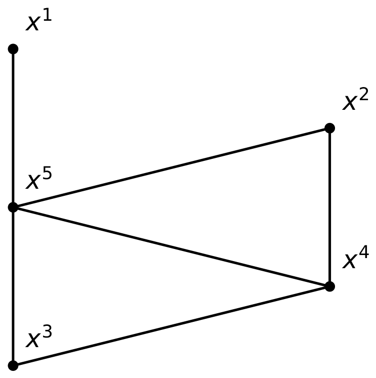
The graph $\Gamma \left(S_M\right)$ for $n=5$ is shown in Figure 1.

5.2. Example B: $n=$ 6 (Even Case)

Here, $n=6=2k$ with $k=3$. By Corollary 4 (a), for

$$t\in \{k+1,\dots ,2k\}=\{4,5,6\},$$

we have

$$\mathrm{CSO}(\Gamma \left(S_M\right))={\displaystyle \sum _{t=4}^6}\left[{\displaystyle \sum _{i=7-t}^3}\left(\sqrt{i^2+{(t-1)}^2}-\sqrt{2}i\right)+{\displaystyle \sum _{i=4}^{t-1}}\left(\sqrt{{(i-1)}^2+{(t-1)}^2}-\sqrt{2}(i-1)\right)\right].$$

Here,

$$L\left(t\right)=7-t,U\left(t\right)=t-1.$$

The index ranges in each nonempty block are given below.

t	$L\left(t\right)=7-t$	$U\left(t\right)=t-1$	active i-ranges
4	3	3	lower: $i=3$;   upper: none
5	2	4	lower: $i=2,3$;   upper: $i=4$
6	1	5	lower: $i=1,2,3$;   upper: $i=4,5$

Thus,

$$\begin{array}{cc}\hfill \mathrm{CSO}\left(\Gamma \left(S_M\right)\right)& =\underset{t=4,i=3}{\underbrace{\left(\sqrt{3^2+3^2}-\sqrt{2}·3\right)}}\hfill \\ & +\underset{t=5,i=2,3}{\underbrace{\left(\sqrt{2^2+4^2}-\sqrt{2}·2\right)+\left(\sqrt{3^2+4^2}-\sqrt{2}·3\right)}}\hfill \\ & +\underset{t=5,i=4}{\underbrace{\left(\sqrt{{(4-1)}^2+4^2}-\sqrt{2}·(4-1)\right)}}\hfill \\ & +\underset{t=6,i=1,2,3}{\underbrace{\left(\sqrt{1^2+5^2}-\sqrt{2}·1\right)+\left(\sqrt{2^2+5^2}-\sqrt{2}·2\right)+\left(\sqrt{3^2+5^2}-\sqrt{2}·3\right)}}\hfill \\ & +\underset{t=6,i=4,5}{\underbrace{\left(\sqrt{{(4-1)}^2+5^2}-\sqrt{2}·(4-1)\right)+\left(\sqrt{{(5-1)}^2+5^2}-\sqrt{2}·(5-1)\right)}}.\hfill \end{array}$$

Numerically, this evaluates to

$$\mathrm{CSO}\left(\Gamma \left(S_M\right)\right)\approx 13.322863493.$$

This agrees with the value obtained by direct edge enumeration and follows directly from Corollary 4.

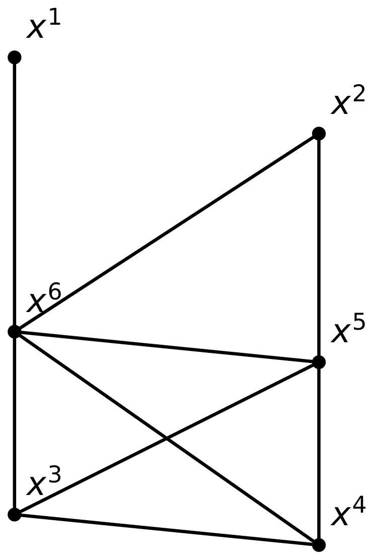
The graph $\Gamma \left(S_M\right)$ for $n=6$ is shown in Figure 2.

6. Extremal and Structural Properties of the CSO Index

In this section, we investigate the structural behavior of the Contrastive Sombor Index and demonstrate that it reflects the degree imbalance between adjacent vertices. In contrast to magnitude-based indices, the CSO index captures local irregularity across edges. We first analyze the contribution of a single edge and then derive global consequences for the graph structure.

Lemma 2.

Let G be a simple graph. For an edge $uv\in E\left(G\right)$, define

$$f(d\left(u\right),d\left(v\right))=\sqrt{d{\left(u\right)}^2+d{\left(v\right)}^2}-\sqrt{2}\min \{d\left(u\right),d\left(v\right)\}.$$

Fix the smaller endpoint degree

$$s=\min \left\{d\right(u),d(v\left)\right\}.$$

Then, $f\left(d\right(u),d(v\left)\right)$ is strictly increasing with respect to the larger endpoint degree. In particular, among edges having the same smaller endpoint degree, an edge with a larger degree difference contributes more to the Contrastive Sombor Index.

Proof. 

Let $uv\in E\left(G\right)$ and assume, without loss of generality, that

$$d\left(u\right)\ge d\left(v\right).$$

Fix the smaller endpoint degree $d\left(v\right)=s$ and write

$$x=d\left(u\right),x\ge s.$$

Then, the contribution of the edge $uv$ to $\mathrm{CSO}\left(G\right)$ is given by

$$g_s\left(x\right)=\sqrt{x^2+s^2}-\sqrt{2}s.$$

Differentiating with respect to x, we obtain

$$g_s^{\prime }\left(x\right)={\displaystyle \frac{x}{\sqrt{x^2+s^2}}}.$$

Since the endpoints of an edge have positive degrees, $x>0$. Therefore,

$$g_s^{\prime }\left(x\right)>0,$$

and hence $g_s\left(x\right)$ is strictly increasing in x.

Consequently, among edges having the same smaller endpoint degree, the edge with the larger endpoint degree contributes more to the Contrastive Sombor Index. Equivalently, within a fixed smaller-degree class, increasing the degree difference increases the corresponding edge contribution.

If $d\left(u\right)=d\left(v\right)=r$, then

$$f(r,r)=\sqrt{2r^2}-\sqrt{2}r=0.$$

Thus, edges joining vertices of equal degree make no contribution to the Contrastive Sombor Index. □

Remark 3.

Lemma 2 shows that, when the smaller endpoint degree is fixed, the CSO contribution increases strictly with the larger endpoint degree. Thus, within each fixed smaller-degree class, edges with greater degree imbalance make larger contributions.

More generally, the CSO contribution depends on both the degree difference and the scale of the endpoint degrees. Therefore, it should not be regarded as a function of $\left|d\right(u)-d(v\left)\right|$ alone. This combined dependence allows the CSO index to reflect both local degree imbalance and endpoint-degree magnitude.

We now recall the decomposition established in Theorem 3 and briefly interpret its structural components.

Remark 4.

By Theorem 3, the CSO index is expressed in terms of the Sombor index $\mathrm{SO}\left(G\right)$, the first Zagreb index $M_1\left(G\right)$, and the total edgewise degree irregularity

$$\sum _{uv\in E\left(G\right)}|d\left(u\right)-d\left(v\right)|.$$

Thus, CSO may be interpreted as a hybrid degree-based invariant combining information on endpoint-degree magnitude, degree intensity, and local degree imbalance.

7. Discrimination Power and Numerical Illustration of the CSO Index

To illustrate the descriptive behavior and structural sensitivity of the proposed Contrastive Sombor Index (CSO), we compute its values for the 18 structural isomers of octane ($C_8{H}_{18}$). This standard dataset provides a convenient numerical example for examining the behavior of degree-based indices under different branching patterns.

In accordance with the classical framework of Gutman and Tošović [16], each molecular graph is represented through its edge-degree distribution. For each pair $(i,j)$, we denote by $n_{ij}$ the number of edges connecting vertices of degrees i and j. This representation allows for efficient computation of degree-based indices without explicit graph reconstruction.

Using this approach, the Sombor index and the Contrastive Sombor Index can be computed as

$$SO\left(G\right)=\sum _{i,j}{n}_{ij}\sqrt{i^2+j^2},$$

and

$$CSO\left(G\right)=\sum _{i,j}{n}_{ij}\left(\sqrt{i^2+j^2}-\sqrt{2}\min \{i,j\}\right).$$

The computed values for all isomers are presented in

Table 2. Edge-degree frequencies, Sombor index (SO), and Contrastive Sombor Index (CSO) values for octane isomers.

No	Name	${\mathit{n}}_{12}$	${\mathit{n}}_{13}$	${\mathit{n}}_{14}$	${\mathit{n}}_{22}$	${\mathit{n}}_{23}$	${\mathit{n}}_{24}$	${\mathit{n}}_{33}$	${\mathit{n}}_{34}$	SO	CSO
1	n-octane	2	0	0	5	0	0	0	0	18.6143	1.6437
2	2-methylheptane	1	2	0	3	1	0	0	0	20.6515	5.0951
3	3-methylheptane	2	1	0	2	2	0	0	0	20.5024	4.9460
4	4-methylheptane	2	1	0	2	2	0	0	0	20.5024	4.9460
5	3-ethylhexane	3	1	0	1	2	0	0	0	19.9100	5.7679
6	2,2-dimethylhexane	1	0	3	2	0	1	0	0	24.7344	10.5922
7	2,3-dimethylhexane	1	2	0	1	2	0	1	0	22.8428	5.8722
8	2,4-dimethylhexane	2	2	0	1	1	1	0	0	21.7028	7.5607
9	2,5-dimethylhexane	0	4	0	1	2	0	0	0	22.6886	8.5465
10	3,3-dimethylhexane	2	0	2	1	0	2	0	0	24.4910	10.3489
11	3,4-dimethylhexane	2	2	0	0	2	0	1	0	22.2504	6.6941
12	3-ethyl-2-methylpentane	2	2	0	0	2	0	1	0	22.2504	6.6941
13	3-ethyl-3-methylpentane	3	0	1	0	0	3	0	0	24.2477	10.1056
14	2,2,3-trimethylpentane	0	2	3	0	1	0	0	1	27.2994	13.1573
15	2,2,4-trimethylpentane	1	1	3	0	1	1	0	0	25.8453	13.1174
16	2,3,3-trimethylpentane	0	2	3	0	1	0	0	1	27.2994	13.1573
17	2,3,4-trimethylpentane	1	4	0	0	0	0	2	0	23.3705	7.8141
18	2,2,3,3-tetramethylbutane	0	0	6	0	0	0	0	1	29.7386	17.0107

.

The values in Table 2 provide a numerical illustration of the response of CSO to different edge-degree distributions. For n-octane, the molecular graph is the path $P_8$. Its edge-degree distribution consists of two edges of type $(1,2)$ and five edges of type $(2,2)$. Since edges of type $(2,2)$ make no contribution to CSO, we obtain

$$CSO\left(P_8\right)=2\left(\sqrt{1^2+2^2}-\sqrt{2}\right)=2\left(\sqrt{5}-\sqrt{2}\right)\approx 1.6437.$$

This is the smallest CSO value among the octane isomers listed in Table 2.

At the other end of the table, the molecular graph of 2,2,3,3-tetramethylbutane has six edges of type $(1,4)$ and one edge of type $(3,4)$. Consequently,

$$\begin{array}{cc}\hfill CSO\left(G\right)& =6\left(\sqrt{1^2+4^2}-\sqrt{2}\right)+\left(\sqrt{3^2+4^2}-3\sqrt{2}\right)\hfill \\ & =6\left(\sqrt{17}-\sqrt{2}\right)+\left(5-3\sqrt{2}\right)\approx 17.0107.\hfill \end{array}$$

This is the largest CSO value in the table. These two examples illustrate how different edge-degree distributions produce different CSO values.

It is important to note that CSO is completely determined by the edge-degree frequencies $n_{ij}$. Therefore, non-isomorphic molecular graphs having the same edge-degree distribution also have the same CSO value. For example, the following pairs are not distinguished by CSO:

$$\begin{array}{cc}& \text{3-methylheptane}\mathrm{and}\text{4-methylheptane},\hfill \\ & \text{3,4-dimethylhexane}\mathrm{and}\text{3-ethyl-2-methylpentane},\hfill \\ & \text{2,2,3-trimethylpentane}\mathrm{and}\text{2,3,3-trimethylpentane}.\hfill \end{array}$$

Thus, the octane data should be interpreted as a numerical illustration of the discrimination behavior of CSO, rather than as evidence of a relationship with a physicochemical property. Establishing such a relationship would require an independent QSPR analysis involving experimental property data, statistical validation, and comparison with existing molecular descriptors.

8. Conclusions

In this study, we introduced the Contrastive Sombor Index and showed that $CSO\left(G\right)=0$ if and only if every connected component of G is regular. We established general lower and upper bounds for the index and derived a decomposition formula expressing CSO in terms of the Sombor index, the first Zagreb index, and the total edgewise degree irregularity.

For monogenic semigroup graphs, we developed a block summation formula and verified it by direct edge enumeration for $n=4,5,6,$ and 7. We also established the asymptotic relation

$$CSO(\Gamma \left(S_M\right))=c{n}^3+O\left(n^2\right),c\approx 0.0705523929.$$

In addition, we investigated the extremal behavior of CSO and proved that the star graph uniquely maximizes the index among all trees of a fixed order. The octane-isomer data were used as a numerical illustration of the discrimination behavior of the index, while the investigation of possible relationships with physicochemical properties is left for future QSPR studies.

Overall, the CSO index provides a complementary measure of structural irregularity alongside the Sombor index by explicitly capturing edgewise deviations from local regularity. From a broader perspective, the Contrastive Sombor Index may be useful for analyzing graphs with different patterns of local irregularity, suggesting potential applications in the study of structural heterogeneity in graph-based models.

Future work may address graph operations, product structures, and extremal problems for CSO. In particular, characterizing the graphs that maximize or minimize CSO under fixed order, degree constraints, or prescribed degree sequences remains an open problem.