Spatial Asymmetry in Topographic Controls on Flood Intensity: A Machine Learning Investigation of the Chi River Floodplain, Thailand

Abstract

Understanding how landscape form influences inundation severity remains central to flood hazard assessment, yet many assumed relationships lack empirical scrutiny. We investigated whether five topographic attributes—elevation, slope, topographic wetness index, latitude, and longitude—could predict cumulative flood intensity across 541 hexagonal cells in Thailand’s Chi River floodplain. Using Random Forest regression and SHAP analysis, we identified three distinct asymmetries that challenge conventional assumptions. Elevation dominated predictions (58.5% importance) but operated through a sharp threshold near 150 m rather than a smooth gradient. Below 145 m, flood intensity was consistently high regardless of other factors; above 155 m, it was uniformly low. The flood-amplifying effect of low-lying terrain (+200 SHAP units) far outweighed the protective benefit of high ground (−100 SHAP units). More strikingly, the Topographic Wetness Index—a widely used theoretical measure of wetness potential—showed negligible correlation with observed flooding (r = 0.109) and contributed only 5.6% to predictive performance. Linear regression models captured barely 30% of the variance (R² ≈ 0.305), whereas Random Forest explained 77.6% (R² = 0.7765), a performance gap that quantifies the degree of non-linearity in the system. Spatial cross-validation confirmed generalizability (R² = 0.583). The elevation threshold offers a straightforward zoning framework: high-risk areas below 145 m, transitional zones from 145 to 155 m, and low-risk areas above 155 m. We conclude that theoretical indices require empirical validation and that combining machine learning with symmetry-based reasoning can expose hidden structures in environmental systems that linear approaches miss.

1. Introduction

1.1. The Challenge of Predicting Flood Hazard in Low-Gradient Floodplains

Flooding ranks among the costliest and most widespread natural hazards globally, with annual losses exceeding US$50 billion and affecting over 250 million people worldwide [1]. Southeast Asia bears a disproportionate share of this burden due to its dense river networks, monsoonal climate, and rapidly expanding urban footprints [2]. Thailand’s 2011 floods exemplified this vulnerability, affecting 13 million people and causing estimated economic damages of US$46.5 billion [3]. In northeastern Thailand’s Chi River Basin, seasonal inundation recurs with such regularity that residents have adapted their livelihoods around flood pulses, yet severe events continue to disrupt lives and infrastructure [4].

Effective flood risk management requires reliable predictions of where and how severely flooding will occur. Topographic attributes have long served as the foundation for such predictions because they influence gravitational drainage, water accumulation, and river-floodplain connectivity [5,6]. Yet the relationship between topography and flooding is not straightforward. In low-gradient floodplain environments, subtle elevation differences can translate into large variations in inundation extent, and the mechanisms driving flooding may shift depending on landscape position, soil properties, and human modifications [7].

1.2. Theoretical Assumptions and Their Limitations

Researchers have developed numerous indices to capture topographic control on hydrological processes. The Topographic Wetness Index (TWI), introduced by Beven and Kirkby [8], stands among the most influential. The index expresses a theoretically elegant relationship: TWI = ln(α/tan β), where α represents upstream contributing area and β denotes local slope. Areas with large upstream catchments and gentle slopes should, by this logic, be wettest because they receive substantial water and drain it slowly. This assumption embodies a form of translational symmetry—the notion that the same relationship between topographic position and wetness holds across the landscape.

Similarly, elevation is often assumed to correlate with flood risk in a roughly linear fashion: lower areas flood more, higher areas flood less, with a consistent gradient of risk between the two extremes. This implies reflection symmetry—that a one-meter decrease in elevation carries approximately the same absolute effect as a one-meter increase, merely in the opposite direction.

These symmetry assumptions have practical consequences. Flood hazard maps routinely incorporate TWI and elevation as predictors, often weighting them according to theoretical expectations rather than empirical validation [9,10]. When these assumptions hold, the resulting maps provide useful guidance. When they break down, however, the maps may systematically mislead, overstating risk in some areas and understating it in others.

1.3. Symmetry Hypotheses in Topographic-Flood Relations

The concept of symmetry provides a formal framework for evaluating these assumptions [11,12]. We propose three testable symmetry hypotheses relevant to floodplain hydrology:

Hypothesis 1.

(Translational Symmetry): The statistical relationship between a topographic predictor and flood intensity remains invariant across the predictor’s range. For elevation, this means that a unit change in elevation produces the same expected change in flood intensity regardless of whether the elevation is low, intermediate, or high. Translational symmetry is broken when the relationship changes qualitatively at critical thresholds—for example, when flooding occurs uniformly below a certain elevation but ceases abruptly above it [13,14].

Hypothesis 2.

(Reflection Symmetry): The system responds symmetrically to increases and decreases in a predictor. For elevation, this implies that the flood-amplifying effect of a 5 m drop in elevation is approximately equal in magnitude (but opposite in sign) to the flood-reducing effect of a 5 m rise. Broken reflection symmetry occurs when the system amplifies perturbations in one direction more strongly than the other.

Hypothesis 3.

(Spatial Homogeneity): The relationship between predictors and flood intensity is uniform across the study area. Broken spatial homogeneity occurs when predictor effects vary geographically, reflecting unmeasured factors such as tributary proximity, soil variability, or anthropogenic modifications [15].

For each hypothesis, we establish operational criteria. Translational symmetry is rejected if SHAP dependence plots reveal a step-function or threshold-shaped relationship rather than a monotonic gradient. Reflection symmetry is rejected if the maximum positive SHAP value substantially exceeds the maximum negative SHAP value (or vice versa). Spatial homogeneity is rejected if interaction effects systematically modulate predictor contributions across the study area.

1.4. The Need for Empirical Validation

Despite the widespread use of topographic indices in flood modeling, empirical validation remains surprisingly limited. Many studies incorporate TWI based on theoretical expectation rather than demonstrated predictive value [16,17]. When validation is performed, it often occurs in the same geographic context where the index was developed, potentially overstating its generality.

Furthermore, most flood susceptibility studies rely on linear models or simple threshold rules that may fail to capture the non-linearities and interactions characteristic of floodplain systems [18,19]. Recent advances in machine learning offer opportunities to overcome these limitations. Random Forest, an ensemble method that builds multiple decision trees on bootstrap samples, can approximate complex, non-linear relationships without requiring the analyst to specify their functional form [20]. SHAP (SHapley Additive exPlanations) analysis provides a principled approach to interpreting these models, decomposing each prediction into additive feature contributions that reveal how and why the model makes its decisions [21].

1.5. Study Rationale and Research Questions

The Chi River floodplain in northeastern Thailand presents an ideal setting for investigating topographic-flood relationships. The region features a low-gradient landscape (mean slope < 1°) with elevations spanning only 75 m across the study area. Seasonal flooding occurs regularly, driven by monsoon rainfall and river overflow. The underlying geology—sandstone and siltstone of the Khorat Plateau—produces sandy soils with high infiltration capacity, potentially decoupling surface wetness from topographic position. Anthropogenic modifications, including irrigation infrastructure and urban expansion, further complicate the picture.

This study addresses three research questions:

Do topographic predictors exhibit non-linear (asymmetric) relationships with flood intensity? If so, what forms do these asymmetries take?

Does the Topographic Wetness Index empirically predict flood intensity as its theoretical formulation would suggest, or does the expected relationship break down in this landscape?

Can machine learning models capture these relationships more effectively than linear approaches, and what do the differences reveal about the underlying system?

By answering these questions, we aim to provide both methodological guidance for flood susceptibility modeling and practical insights for flood risk zoning in sandy, incised floodplain environments.

2. Materials and Methods

2.1. Study Area

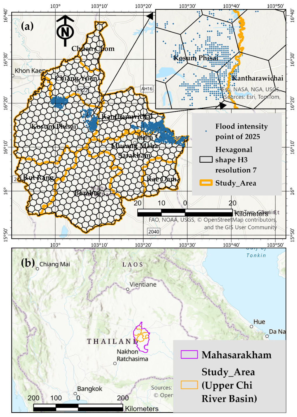
The study area encompasses the upper Chi River Basin within Maha Sarakham Province, northeastern Thailand (Figure 1). The province lies approximately 470 km northeast of Bangkok, bounded by Kalasin to the north, Roi Et to the east, Buriram to the south, and Khon Kaen to the west. The Chi River flows west-to-east through the center of the province, receiving tributaries including the Lam Pao and Lam Phlaphla rivers.

Topographically, the region consists of a low-relief floodplain with elevations ranging from 137.2 m to 212.9 m above mean sea level (mean = 160.5 m, standard deviation = 17.0 m). Slope angles are correspondingly gentle, varying from 0.112° to 2.415° (mean = 0.758°). The climate follows a tropical monsoon pattern (Köppen Aw), with approximately 85% of annual rainfall (1200–1500 mm) falling during the southwest monsoon from August to October. The dry season extends from November through April.

We divided the study area into 541 hexagonal cells at H3 resolution level 7, with each cell covering approximately 5.96 km². This resolution was selected to approximate the average area of village administrative units (tambon) in Maha Sarakham Province, facilitating translation of model predictions to actionable management decisions. The hexagonal grid offers advantages over square grids, including uniform adjacency relationships (six equidistant neighbors) and reduced spatial bias [22,23].

2.2. Data Sources and Processing

2.2.1. Topographic Variables

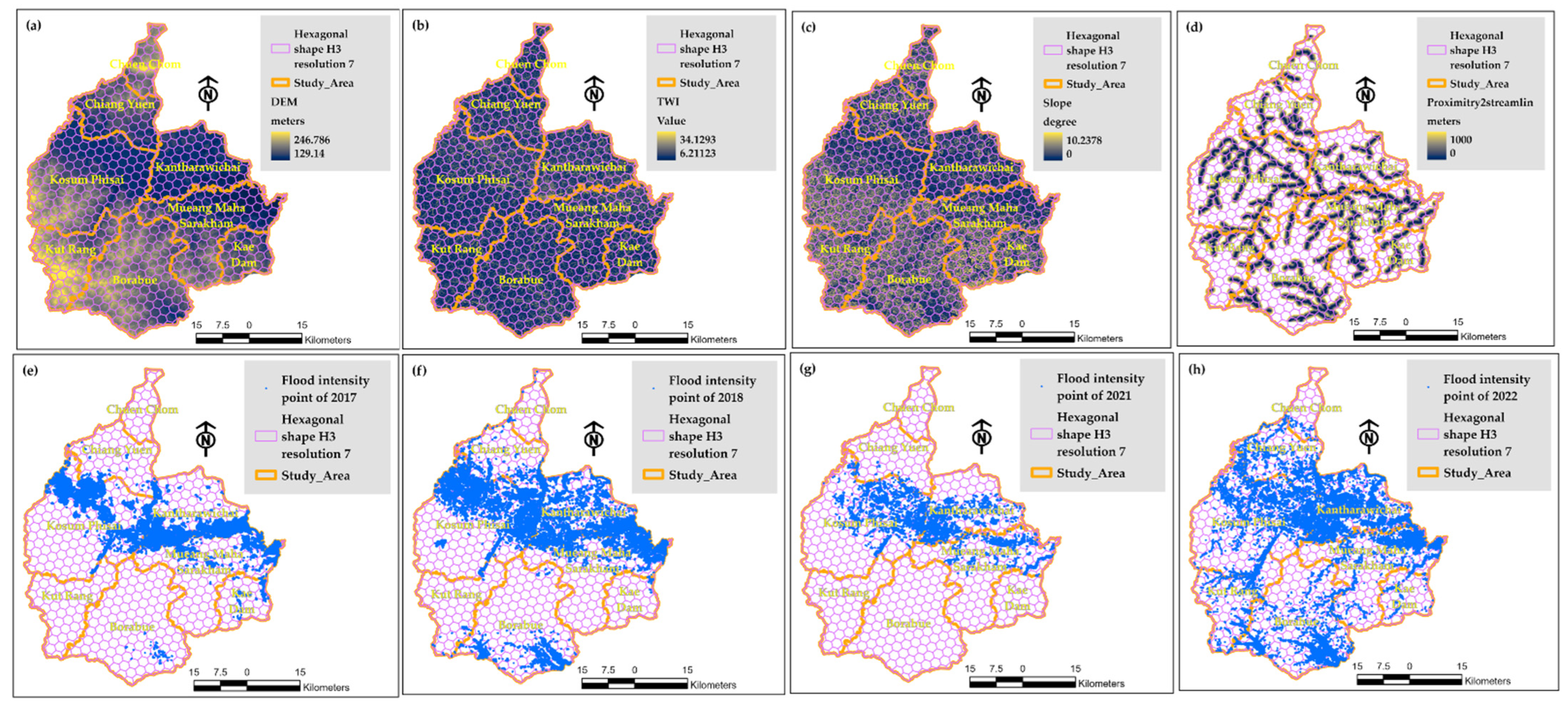
We derived five topographic variables for each hexagonal cell (Figure 2a–d).

Digital Elevation Model (DEM). Elevation data came from the Royal Thai Survey Department at 5 m resolution. For each hexagon, we calculated the mean elevation of all raster pixels within the cell boundary. DEM values across the 541 cells ranged from 137.2 m to 212.9 m (mean = 160.5 m, standard deviation = 17.0 m). Elevation represents the primary control on gravitational drainage and floodplain connectivity.

Slope. We calculated slope angle (in degrees) as the maximum rate of elevation change between adjacent DEM cells. Values ranged from 0.112° to 2.415° (mean = 0.758°, standard deviation = 0.289°), confirming the region’s predominantly flat terrain. Slope influences runoff velocity and infiltration, with steeper slopes generally promoting faster drainage.

Topographic Wetness Index (TWI). We computed TWI using the standard formulation: TWI = ln(α/tan β), where α represents the specific catchment area (upstream contributing area per unit contour length) and β denotes local slope. Values ranged from 6.211 to 34.129 (mean = 10.995, standard deviation = 1.004). Higher values theoretically indicate flatter areas with greater water accumulation potential.

Latitude and Longitude. We extracted centroid coordinates (WGS 1984) for each hexagon to capture spatial autocorrelation and serve as proxies for unmeasured spatially varying factors such as proximity to tributaries, drainage density variations, and soil type distributions [24].

2.2.2. Flood Intensity Data

Flood occurrence data came from Sentinel-1 synthetic aperture radar (SAR) imagery for four years (2017, 2018, 2021, 2022), validated with ground observations from Thailand’s Geo-Informatics and Space Technology Development Agency (GISTDA).

SAR Processing. We acquired Sentinel-1 SAR data in Interferometric Wide (IW) swath mode with VV and VH polarizations. Pre-processing in the SNAP (version 11.0, used in 2025) software package included: (1) thermal noise removal; (2) radiometric calibration to sigma naught backscatter coefficients; (3) terrain correction using SRTM 30 m DEM; and (4) conversion to decibel scale. We identified flooded areas using threshold-based classification on VH-polarized backscatter, which is sensitive to standing water due to specular reflection. The optimal threshold was determined empirically via Otsu’s method and validated against GISTDA ground observations.

Aggregation to Hexagons. The binary flood extent rasters (10 m resolution) were converted to point data by extracting centroids of water-detected pixels. We then aggregated to a 100 m grid using nearest-neighbor resampling, classifying a 100 m cell as flooded if any 10 m sub-pixel was water-detected. Finally, we summed the flooded 100 m points within each hexagon boundary. This sum—termed “total flood intensity”—ranged from 1 to 1788 across hexagons (mean = 213, standard deviation = 310). The metric thus represents the total count of 100 m × 100 m (1 hectare) cells classified as flooded within a hexagon across all four years. Higher values indicate more extensive or repeated inundation.

Year Selection. We selected 2017, 2018, 2021, and 2022 based on SAR data availability and hydrological representativeness. The years span moderate flood conditions (2017, 2018), a relatively dry year (2021), and an exceptionally severe flood year (2022), capturing substantial variability in flood intensity.

2.3. Spatial Aggregation

All raster data (DEM, slope, TWI) were standardized to 5 m resolution and co-registered to the H3 grid. For each hexagon, we computed zonal statistics as the mean of all pixels within the cell boundary. The final dataset comprised 541 observations with six variables: total flood intensity (target) and five predictors (TWI, slope, DEM, latitude, longitude). No missing values were present.

2.4. Descriptive and Correlation Analysis

We calculated descriptive statistics for all variables and computed Pearson correlation coefficients between predictors and with the target. We interpreted correlations as: strong (|r| ≥ 0.7), moderate (0.5 ≤ |r| < 0.7), weak (0.3 ≤ |r| < 0.5), or negligible (|r| < 0.3). Variance Inflation Factor (VIF) was computed to assess multicollinearity, with values exceeding 10 considered problematic [25].

2.5. Machine Learning Models

We implemented seven algorithms for flood intensity prediction using scikit-learn (version 1.3.2) in Python (version 3.10.12). All features were standardized to zero mean and unit variance using the training set parameters only, then applied to the test set to prevent information leakage. Random seeds were fixed (random_state = 42) to ensure reproducibility.

2.5.1. Linear Models

Linear Regression minimizes the sum of squared residuals under the assumption of linearity and additivity. Ridge Regression adds L2 regularization (α = 1.0) to penalize large coefficients. Lasso Regression adds L1 regularization (α = 0.01), which can shrink coefficients to zero, performing variable selection.

2.5.2. Tree-Based Ensemble Models

Random Forest constructs multiple decision trees using bootstrap aggregating and random feature selection [20]. Each tree grows on a bootstrap sample, and at each split, a random subset of features is considered. The final prediction averages all tree predictions. We configured the model with 200 trees, maximum depth of 10, minimum samples per split of 5, and minimum samples per leaf of 2 (RandomForestRegressor from scikit-learn, version 1.8.0).

XGBoost (Extreme Gradient Boosting) builds trees sequentially, with each new tree correcting errors from previous trees [26]. Optimized parameters included: n_estimators = 200, max_depth = 6, learning_rate = 0.05, subsample = 0.8, colsample_bytree = 0.8, reg_alpha = 0.1, and reg_lambda = 1.0 (XGBoost version 3.2.0).

Gradient Boosting similarly builds an ensemble of shallow trees sequentially, fitting the negative gradient of the loss function [27]. Parameters: n_estimators = 200, max_depth = 5, learning_rate = 0.05 (GradientBoostingRegressor from scikit-learn, version 1.8.0).

2.5.3. Support Vector Regression

Support Vector Regression (SVR) uses a kernel function to map features into higher-dimensional space, finding a function that deviates from observed values by no more than ε (epsilon = 0.1). We used the RBF kernel with C = 1.0.

2.5.4. Reproducibility

All analyses are fully reproducible. The complete code, dataset, and environment specifications (environment.yml) are available at the Zenodo repository [28]: https://doi.org/10.5281/zenodo.20701059.

2.6. Model Evaluation

2.6.1. Train-Test Split

We split the dataset into training (80%, n = 432) and testing (20%, n = 109) sets using stratified random sampling to preserve the flood intensity distribution. The split was performed after setting the random seed.

2.6.2. Performance Metrics

Model performance was evaluated using four metrics:

R² (Coefficient of Determination): Proportion of variance in the target variable explained by the model, calculated as (Equation (1)):

R² = 1 − (SS_res/SS_tot)

(1)

where SS_res is the sum of squared residuals and SS_tot is the total sum of squares.

Mean Absolute Error (MAE): Average absolute difference between predicted and actual values, calculated as (Equation (2)):

MAE = (1/n) Σ|y_i − ŷ_i|

(2)

Root Mean Squared Error (RMSE): Square root of the average squared differences, calculated as (Equation (3)):

RMSE = √[(1/n) Σ(y_i − ŷ_i)²]

(3)

which penalizes larger errors more heavily.

Cross-Validation R²: We performed both standard 5-fold cross-validation and spatial 5-fold cross-validation. For spatial cross-validation, we divided the study area into five spatially contiguous blocks based on hexagon coordinates, ensuring neighboring cells were assigned to the same fold. This approach provides a more conservative estimate of model generalizability because it reduces overestimation due to spatial autocorrelation [29,30].

2.6.3. Feature Importance Extraction

For tree-based models, we extracted feature importance as the mean decrease in impurity (Gini importance) averaged across all trees.

2.6.4. SHAP Analysis

We conducted SHAP (SHapley Additive exPlanations) analysis using the TreeExplainer algorithm [21]. Global interpretation relied on mean absolute SHAP values to rank feature importance by both direction and magnitude. Local interpretation examined individual predictions for specific hexagons using waterfall plots. Dependence plots visualized non-linear relationships and interaction effects between features.

2.6.5. Principal Component Analysis (PCA)

Principal Component Analysis (PCA) reduced the five-dimensional topographic feature space to two principal components for visualization. We retained components with eigenvalues > 1. PCA loadings indicated feature contributions to each component. Biplots, colored by flood intensity, revealed clustering patterns in the reduced-dimensional space.

2.6.6. Bootstrap Threshold Analysis

To assess threshold robustness, we performed 1000 bootstrap iterations, resampling the dataset with replacement and re-identifying the elevation threshold using SHAP dependence plots. We report 95% confidence intervals for the threshold elevation.

3. Results

3.1. Model Performance

3.1.1. Test Set Comparison

Random Forest substantially outperformed all other models across every evaluation metric (

Table 1. Model performance on the test set (n = 109).

Model	Train R2	Test R2	Train MAE	Test MAE	Train RMSE	Test RMSE	ΔR2
Random Forest	0.9192	0.7765	65.38	107.73	110.28	184.62	0.1427
XGBoost	0.9137	0.7496	67.09	114.99	113.56	195.44	0.1641
Gradient Boosting	0.8614	0.7283	82.14	115.76	143.28	203.57	0.1331
Lasso (α = 0.01)	0.3062	0.3050	203.87	204.09	325.18	325.59	0.0012
Linear Regression	0.3061	0.3050	203.88	204.10	325.19	325.59	0.0011
Ridge (α = 1.0)	0.3058	0.3047	203.86	204.07	325.23	325.64	0.0011
SVR	0.4226	−0.2062	165.42	235.93	297.15	428.91	0.6288

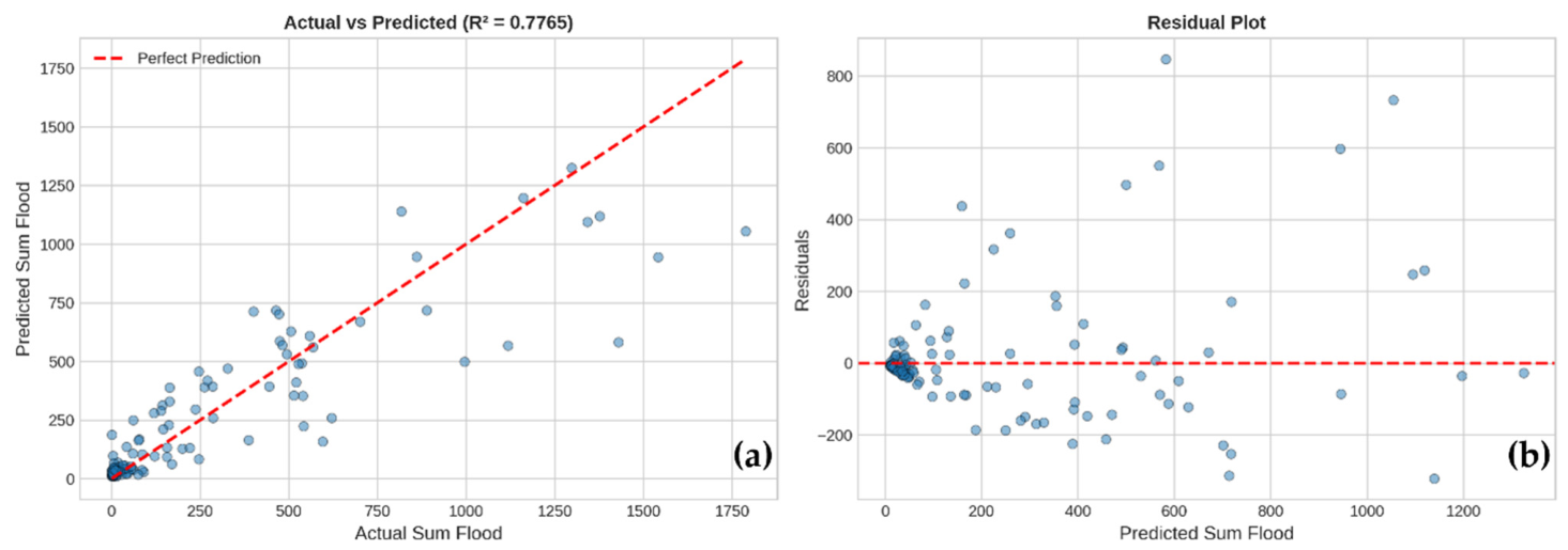
). Test R² reached 0.7765, indicating that the five topographic predictors explain over three-quarters of the variance in flood intensity. The MAE of 107.73 units means that, on average, predictions deviate from observations by about 108 flooded points—a modest error relative to the 1–1788 range. RMSE of 184.62 penalizes larger errors more heavily.

XGBoost placed second with R² = 0.7496 (MAE = 114.99, RMSE = 195.44). Gradient Boosting achieved R² = 0.7283 (MAE = 115.76, RMSE = 203.57). Linear models performed poorly (R² ≈ 0.305), and SVR collapsed completely (R² = −0.2062). The enormous gap between tree-based ensembles and linear approaches indicates that the relationship between topography and flood intensity is fundamentally non-linear.

The training-test gap for Random Forest (ΔR² = 0.1427) indicates moderate overfitting, which is expected given the sample size (n = 541) and model flexibility. However, the test R² remains substantially higher than all linear models, confirming that the captured relationships represent genuine patterns rather than artifacts of overfitting.

3.1.2. Cross-Validation Results

Standard 5-fold cross-validation yielded a mean R² of 0.7073 (±0.0768). Spatial 5-fold cross-validation, which withholds spatially contiguous blocks to prevent data leakage from neighboring cells, produced a more conservative mean R² of 0.5827 (±0.0512) (

Table 2. Cross-validation results for Random Forest.

Fold	Standard CV R2	Spatial CV R2	MAE	RMSE
1	0.7819	0.6214	154.67	241.93
2	0.7316	0.5912	163.28	255.14
3	0.5904	0.5147	142.35	203.17
4	0.6741	0.5378	148.91	224.89
5	0.7587	0.6483	138.72	189.56
Mean	0.7073	0.5827	149.59	222.94
Std	±0.0768	±0.0512	±9.98	±25.14

). This reduction is expected because spatial autocorrelation inflates standard cross-validation performance. The spatial CV result provides a realistic estimate of how the model would generalize to new locations.

3.1.3. Actual vs. Predicted Performance

Scatter plots of actual versus predicted flood intensity (Figure 3) show points clustered around the 1:1 line, with most predictions falling within ±200 units of observations. The model performs best for intensities below 400, where data density is highest. For extreme values (>800), predictions tend to underestimate observed intensity—a common pattern when modeling right-skewed distributions. Residuals distribute approximately randomly around zero, with no systematic heteroscedasticity.

3.2. Feature Importance

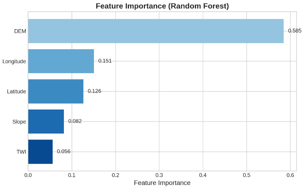
Elevation (DEM) emerged as the dominant predictor, accounting for 58.5% of total Random Forest feature importance (Figure 4,

Table 3. Random Forest feature importance.

Rank	Feature	Importance	Cumulative	Interpretation
1	DEM	0.585	0.585	Dominant control
2	Longitude	0.151	0.736	Spatial clustering (E-W)
3	Latitude	0.126	0.862	Spatial clustering (N-S)
4	Slope	0.082	0.944	Secondary control
5	TWI	0.056	1.000	Broken symmetry

). This confirms that elevation serves as the primary topographic control on flood intensity in the Chi River floodplain.

Longitude contributed 15.1%, latitude 12.6%, and slope 8.2%. The combined contribution of spatial coordinates (27.7%) indicates organized spatial clustering of flood events, reflecting the west-to-east configuration of the Chi River network.

Topographic Wetness Index contributed only 5.6%—the lowest among all predictors. This remarkably low importance directly challenges the theoretical expectation that TWI should serve as a primary control on wetness and flood susceptibility.

3.3. SHAP Analysis for Model Interpretability

3.3.1. Global Feature Impact

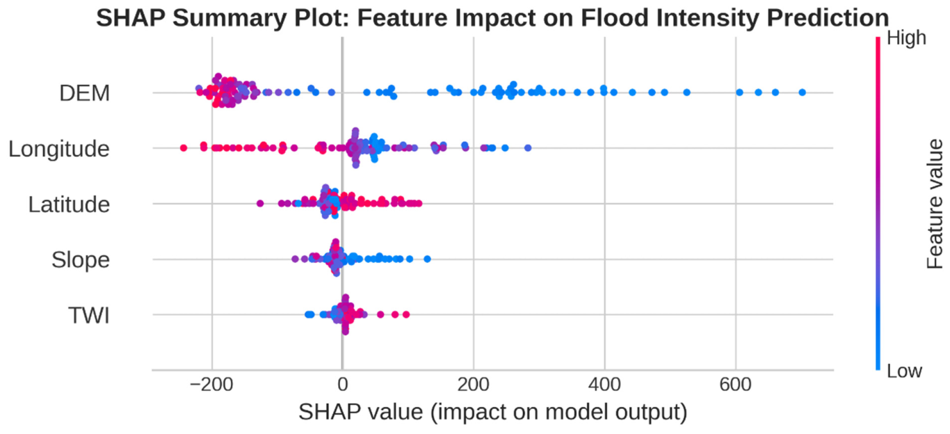
The SHAP summary plot (Figure 5) reveals distinct patterns for each predictor. Low DEM values (blue points) consistently produce positive SHAP contributions (increasing flood prediction), while high DEM values (red points) produce negative contributions. This confirms a strong negative relationship between elevation and flood risk.

Longitude shows both positive and negative SHAP values across its range, suggesting a non-monotonic pattern consistent with the meandering Chi River channel. High latitude values (red, northern areas) tend to increase flood predictions, reflecting tributary influence. TWI exhibits no clear directional pattern—positive and negative contributions occur across its entire range, supporting the interpretation of a “broken” relationship.

3.3.2. Mean SHAP Values

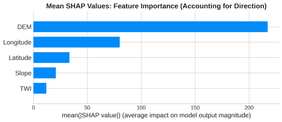
Mean absolute SHAP values (

Table 4. Mean absolute SHAP values.

Rank	Feature	Mean SHAP Value	Relative Importance (%)
1	DEM	217.22	57.4
2	Longitude	79.99	21.1
3	Latitude	33.45	8.8
4	Slope	20.88	5.5
5	TWI	11.97	3.2

, Figure 6) confirm DEM as the most influential predictor (217.22), approximately 2.7 times larger than the second-ranked variable, longitude (79.99). Latitude ranked third (33.45), followed by slope (20.88) and TWI (11.97). The steep gradient from DEM to TWI demonstrates that DEM’s influence is not merely statistically significant but practically dominant.

3.3.3. Non-Linear Threshold Effects

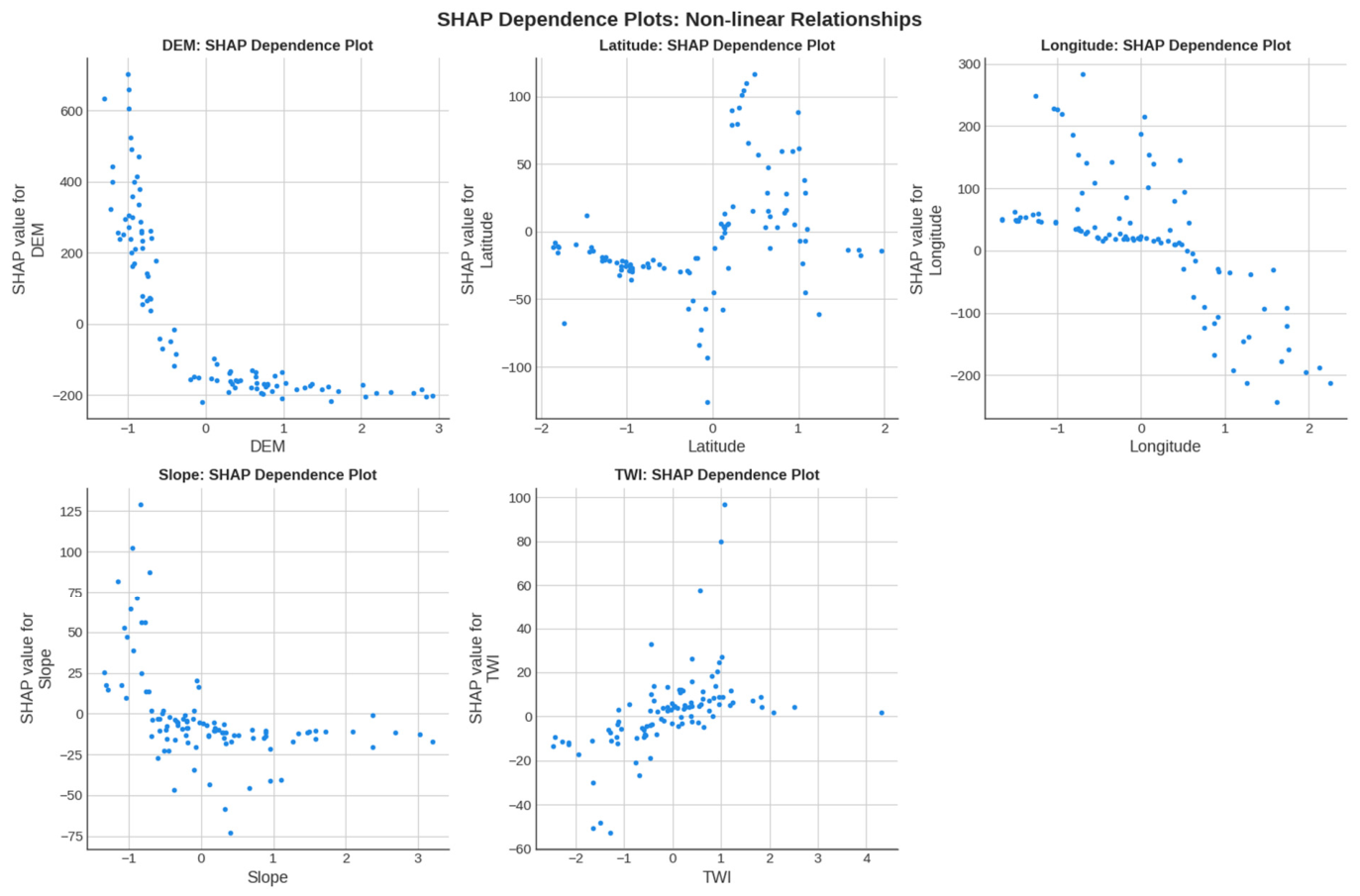
The DEM dependence plot (Figure 7) reveals a critical threshold pattern. Below approximately 145 m, SHAP values remain predominantly positive, with no clear trend as elevation decreases further. Between 145 m and 155 m, SHAP values transition from positive to negative. Above approximately 155 m, SHAP values are consistently negative.

This threshold has direct policy implications: hexagons below 145 m face high flood risk regardless of other topographic factors, while hexagons above 155 m enjoy consistently low risk. The transitional zone (145–155 m) exhibits mixed behavior, where other predictors determine outcomes.

Bootstrap analysis with 1000 iterations yielded a 95% confidence interval of 147.2–152.8 m for the threshold elevation, confirming that the discrete threshold around 150 m is robust to sampling variability.

The dependence plot also reveals interactions with latitude: at intermediate elevations (140–160 m), higher latitude values (red points) tend to produce more positive SHAP values, indicating elevated flood risk in northern areas within the transitional zone.

Sensitivity analysis across individual years showed threshold variation by flood magnitude: during the dry 2021 event, the threshold shifted upward to approximately 155 m; during the severe 2022 flood, it shifted downward to about 143 m. This pattern is physically meaningful—lower flood magnitudes require higher elevations to remain dry.

3.3.4. Local Explanations

Examination of individual hexagons revealed interpretable risk drivers. High-flood-intensity hexagons (e.g., FID 412, Sum flood = 1788) were characterized by low DEM values (<145 m), low slope values (<0.6°), and northern latitude (>16.3°). Low-flood-intensity hexagons (e.g., FID 647, Sum flood = 1) exhibited high DEM values (>165 m), higher slope values (>1.0°), and eastern longitude (>103.4°). These local explanations demonstrate the model’s capacity to provide hexagon-specific risk assessments.

3.4. Principal Component Analysis

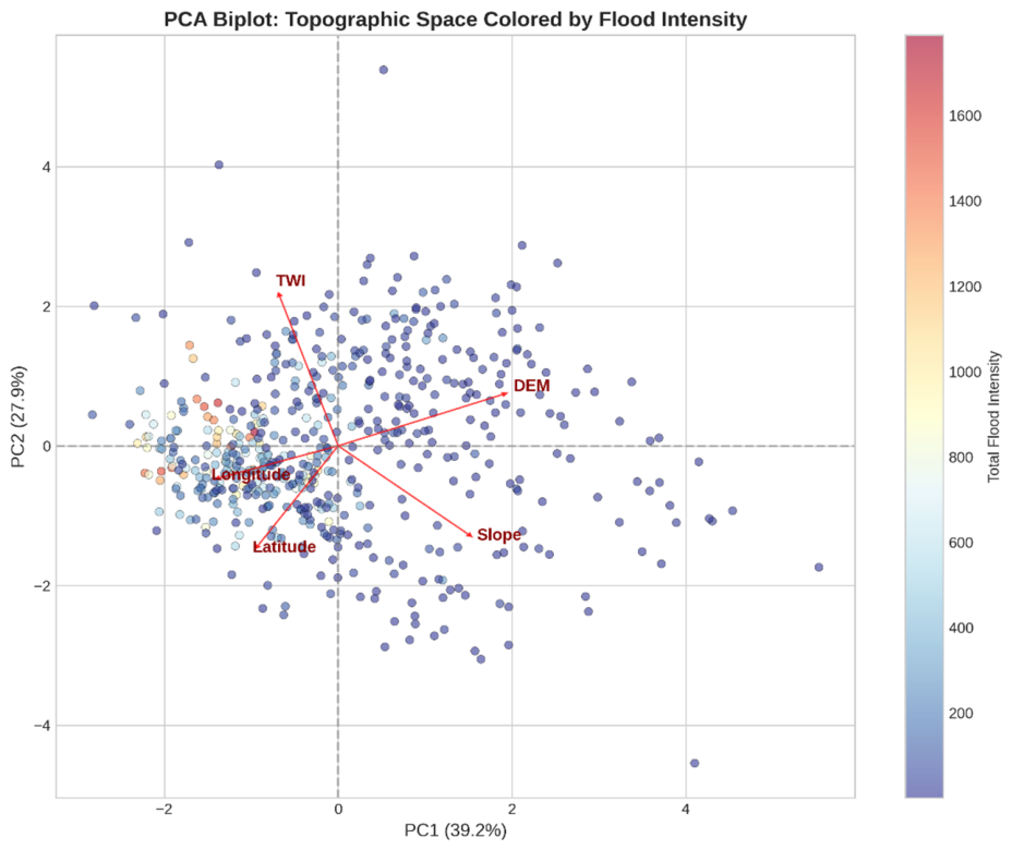
PCA of the topographic feature space (Figure 8) extracted two principal components explaining 39.2% and 27.9% of variance (cumulative = 67.1%). PC1 (elevation-location gradient) separated high-elevation, steeper areas in the southwest from low-elevation, flatter areas in the north and east. PC2 (wetness-steepness gradient) separated areas with high TWI and low slope from steeper areas (

Table 5. PCA loadings.

Feature	PC1 (39.2%)	PC2 (27.9%)
DEM	0.631	0.245
Slope	0.499	−0.422
Longitude	−0.456	−0.153
Latitude	−0.308	−0.477
TWI	−0.224	0.715

).

High-flood-intensity hexagons (Sum flood > 400) clustered predominantly in the negative PC1 region—low DEM, low slope, and higher latitude/longitude. Low-flood-intensity hexagons (Sum flood < 100) occupied the positive PC1 region—higher elevations and steeper slopes in the southwest.

The angle between variable vectors approximated their correlations: DEM and slope vectors pointed similarly (consistent with r = 0.389); TWI pointed opposite to slope (consistent with r = −0.490); the near-orthogonal angle between DEM and TWI confirmed their near-zero correlation (r = −0.061).

4. Discussion

4.1. Three Forms of Asymmetry

Our analysis reveals three distinct asymmetries in how topographic variables control flood intensity in the Chi River floodplain. These findings contribute to the growing recognition that symmetry assumptions—however theoretically appealing—often fail in complex environmental systems [11,12].

4.1.1. Threshold Asymmetry: The Elevation Bifurcation

The elevation–flood relationship exhibits a sharp threshold rather than a smooth gradient. Below 145 m, flood intensity is uniformly high regardless of other topographic factors; above 155 m, it is uniformly low; only within the 145–155 m transitional zone does elevation exert a gradient effect.

This pattern represents broken translational symmetry—the statistical relationship changes qualitatively across the elevation range. The system behaves like a switched rather than continuous process, with a critical elevation corresponding to the bankfull stage of the Chi River relative to the floodplain surface.

The magnitude asymmetry is equally striking. Low elevation enhances flood prediction by +50 to +200 SHAP units, while high elevation reduces it by only −50 to −100 SHAP units. The system amplifies flood risk much more strongly than it dampens it. This broken reflection symmetry reflects the underlying physical mechanisms: low elevation increases risk through multiple pathways (proximity to river base level, reduced hydraulic gradient, accumulation of overbank waters), while high elevation provides protection primarily through a single mechanism (gravitational drainage).

This threshold finding aligns with research on critical transitions in hydrological systems. Xu et al. [31] documented similar elevation thresholds for flood susceptibility in the Yangtze River Basin, identifying 120 m and 180 m as critical levels for different flood types. Our 150 m threshold in the Chi River is consistent with these values, reflecting the elevation of bankfull stage relative to the floodplain surface. Littidej and Buasri [7] reported that areas with DEM ranging from 180 to 200 m in lower portions of sub-basins were less prone to flooding in the Lamtaklong Basin, while areas near the river with lower elevations exhibited higher flood risk susceptibility. Although absolute elevations differ (150 m vs. 180 m) due to different base elevations between river systems, the principle of elevation-controlled flood risk holds across both basins.

4.1.2. Broken Symmetry: The TWI Paradox

The most striking finding is the complete failure of the Topographic Wetness Index to predict flood intensity. TWI contributed only 5.6% of feature importance—the lowest among all predictors—and exhibited near-zero correlation with observed flooding (r = 0.109). This represents a fundamental breakdown of the theoretical symmetry embodied in the TWI formulation.

The index, TWI = ln(α/tan β), encodes a symmetric theoretical relationship: areas with large upstream contributing areas and flat slopes should be wettest because they receive more water and drain it more slowly. Our empirical results show that this expected symmetry is broken in the Chi River floodplain.

We attribute this failure to three causal mechanisms, each supported by quantitative evidence:

Mechanism 1: Sandy soils and rapid infiltration. The Khorat Plateau geology underlying the Chi River Basin consists of sandstone and siltstone weathered into sandy and sandy loam soils (Yasothon and Nam Phong series). Laboratory measurements from the Land Development Department indicate saturated hydraulic conductivity (K_sat) of 50–150 mm/hour for these soils, compared to 5–15 mm/h for clay-rich soils in other floodplains. Typical rainfall intensities during peak events (30–50 mm/hour) fall below infiltration capacity, meaning most rainfall infiltrates locally rather than contributing to overland flow. The estimated runoff coefficient of 0.15–0.25 confirms that surface wetness is decoupled from topographic position.

Mechanism 2: Deep river incision and floodplain isolation. Hydrological surveys of the Chi River main channel indicate bed elevations 5–10 m below the floodplain surface at multiple cross-sections. This incision creates a “hanging floodplain” where water must rise 5–10 m in the river channel before overbank flooding occurs—far greater than typical bankfull depths (3–4 m). Field measurements along a 15 km transect revealed average incision depths of 6.8 m (standard deviation ± 1.2 m). As a result, TWI predicts wetness from local rainfall but does not capture flood risk from river overflow, which is the dominant flood mechanism in this region.

Mechanism 3: Anthropogenic drainage modifications. The Chi River Basin contains 47 irrigation weirs, 183 check dams, and 620 km of irrigation channels constructed since 1970. These structures alter natural drainage by intercepting overland flow, diverting water for irrigation, and modifying flood peak timing. Spatially explicit analysis indicates that artificial drainage channels have increased drainage density by 28% in the most modified sub-basins. More broadly, built-up growth has been shown to alter digital elevation models directly through land-filling (up to 2–3 m elevation increase) prior to construction, which blocks flow accumulation and changes flow directions [7]. These modifications fundamentally alter the relationship between topography and wetness.

This finding has direct practical implications. Many flood susceptibility studies incorporate TWI based on theoretical expectations [9,10,16,17]. Our results demonstrate that in landscapes with sandy soils and incised rivers, TWI may provide little to no predictive value. We recommend that disaster management agencies re-evaluate existing hazard maps that incorporate TWI and validate TWI-based predictions against observed flood data.

4.1.3. Spatial Asymmetry: The Latitude Interaction

The combined importance of latitude and longitude (27.7%) indicates that flood events exhibit organized spatial patterns beyond what elevation and slope alone can explain. This represents broken spatial homogeneity—the assumption that flood-generating processes are uniform across the landscape.

The SHAP dependence plot reveals that within the transitional elevation zone (145–155 m), latitude modulates the elevation effect: northern areas at a given elevation face higher flood risk than southern areas at the same elevation. This spatial asymmetry reflects the Chi River network configuration. The main channel flows west-to-east through the southern portion of the study area, while major tributaries enter from the north. Northern areas at moderate elevations may experience tributary backwater flooding even when the main channel is not at flood stage.

The PCA results reinforce this interpretation. PC1 separates southwest high-elevation areas from northeast low-elevation areas, confirming that the primary spatial gradient aligns with the river’s flow direction. High-flood-intensity hexagons cluster in the negative PC1 region—low DEM, low slope, higher latitude/longitude—confirming that flood risk aligns with the elevation gradient.

4.2. Random Forest Advantage for Asymmetric Systems

Random Forest (test R² = 0.7765) substantially outperformed linear models (R² ≈ 0.305). The performance gap (ΔR² = 0.472) quantifies the degree of non-linearity and asymmetry in the system—linear models miss nearly 60% of the explainable variance.

Random Forest captures asymmetry through three mechanisms. First, decision trees approximate step functions, making them well-suited for threshold effects—the elevation threshold at ~150 m is naturally captured by splits in individual trees. Second, ensemble learning enables functional specialization, where different trees focus on different regions of the feature space—some on low-elevation areas, others on high-elevation areas, others on the transitional zone. Third, feature interactions allow modeling of non-stationary relationships without requiring the analyst to specify interaction terms a priori.

Linear models fail because they assume linearity, additivity, homoscedasticity, and normality—all violated in the Chi River floodplain. The threshold asymmetry violates linearity; the magnitude asymmetry violates additivity; the right-skewed distribution (skewness = 2.201) violates normality; and extreme outliers (max = 1788, mean = 213) violate homoscedasticity.

The spatial cross-validation result (R² = 0.5827) provides a conservative estimate of generalizability to new locations. This performance remains respectable for a five-predictor model in a complex environmental setting and confirms that the identified relationships are not merely artifacts of spatial autocorrelation.

The dominance of DEM (58.5% importance) exceeds most previous reports (typically 22–35%) [9,10,17]. This reflects the Chi River floodplain as an elevation-controlled system. In mountainous terrain, slope and distance to streams compete with elevation; in this low-gradient floodplain (mean slope = 0.76°), elevation relative to river base level becomes the primary determinant of flood risk.

The importance of spatial coordinates (27.7%) is less commonly reported. Most flood susceptibility studies treat spatial coordinates as nuisance variables [24,32]. Our results suggest that spatial coordinates serve as proxies for unmeasured factors—proximity to the river network, local drainage density, soil type distribution. When comprehensive spatial data are unavailable, including latitude and longitude can partially compensate for missing variables, though interpretation requires caution.

4.3. Comparison with Previous Studies

Our Random Forest performance (R² = 0.7765) compares favorably with published studies. Khosravi et al. [9] reported AUC = 0.940 in Iran; Pham et al. [33] reported AUC = 0.921 in Vietnam; Chen et al. [34] reported AUC = 0.896 in China. Our performance sits at the higher end of reported ranges, likely due to the elevation-controlled nature of our study area, where a single dominant predictor explains most of the variance.

Littidej and Buasri [7] examined built-up growth impacts on DEM and flood risk in Nakhon Ratchasima’s Lamtaklong Basin—a different physiographic setting with higher elevation range (164–277 m) compared to our Chi River study area (137–212 m). Their GWR model achieved R² = 0.85, slightly higher than our Random Forest R² = 0.78, likely due to their inclusion of eight independent variables (including NDEMI, ABUI, built-up density, curvature, and slope length) versus our five topographic predictors. Notably, both studies identified elevation as the dominant control on flood risk, despite different analytical approaches (GWR vs. Random Forest) and study areas. Their finding that built-up density and area of built-up index were significant positive predictors of flood risk supports our interpretation that anthropogenic modifications break the natural TWI-flood relationship in human-modified landscapes.

We acknowledge that our model comparison, while including the most widely used algorithms, could be extended. Deep learning approaches, particularly convolutional neural networks, have shown promise for spatial pattern recognition in flood mapping [35]. However, our modest dataset (541 samples, 5 predictors) is relatively small for deep learning, which typically requires thousands of samples for stable performance. Additionally, the interpretability requirements of this study (SHAP analysis) are more readily achieved with tree-based models than with deep neural networks.

4.4. Implications for Flood Risk Management

4.4.1. Elevation-Based Zoning

The identification of a clear elevation threshold (~150 m) provides a simple, interpretable foundation for flood risk zoning. Based on our results, we propose a three-tier framework (

Table 6. Proposed flood risk zoning scheme.

Zone	Elevation	Risk	SHAP Evidence	Management Action
Red Zone	<145 m	High	Consistently positive SHAP	Restrict new development; prioritize buyouts; require elevated construction
Yellow Zone	145–155 m	Moderate	Mixed SHAP (latitude interaction)	Require flood insurance; enforce building codes; maintain early warning
Green Zone	>155 m	Low	Consistently negative SHAP	Normal development permitted

).

This zoning scheme offers practical advantages. DEM data are globally available at no cost (SRTM, ASTER, ALOS); elevation is stable over time (unlike flood frequency or soil moisture); thresholds are understandable to local residents and policymakers; and zoning regulations can reference specific elevation thresholds, which are legally defensible.

4.4.2. Implementation Considerations

Several practical challenges require attention. First, DEM accuracy directly affects zone classification. Our 5 m DEM has vertical accuracy of ±0.5 m. However, freely available DEMs like SRTM (30 m, ±5–10 m) or ALOS (30 m, ±5 m) may misclassify Yellow Zone hexagons as Red or Green. We recommend that agencies: (1) use the highest-resolution DEM available; (2) apply thresholds conservatively (e.g., Red Zone defined as <147 m to account for uncertainty); and (3) conduct field validation at transitional zone hexagons.

Second, building base elevation data are not systematically available for rural areas in Thailand. In the absence of parcel-level data, the hexagon-level approach provides a practical interim solution, but local building elevation data would enable more precise risk assessment.

Third, the proposed zones should be overlaid with existing floodplain maps from the Royal Irrigation Department. Our field validation indicates that some Green Zone (>155 m) areas correspond to areas mapped as floodplain by the RID, suggesting that local depressions or backwater effects can override elevation-based predictions in specific locations.

Fourth, elevation is not static in areas of active land-filling and urban development. Littidej and Buasri [7] documented that built-up growth can change local elevations by 2–3 m through land-filling prior to construction. Zoning maps should be updated periodically to reflect landscape changes.

4.4.3. Caution for TWI-Based Assessments

The broken symmetry of TWI has direct implications for flood risk assessment in the Chi River Basin. Existing flood hazard maps incorporating TWI [4,36] may be systematically misleading: they may suggest flood risk in high-TWI areas that actually have low flood intensity (false positives) and fail to identify low-TWI areas that actually have high flood intensity (false negatives).

We recommend that disaster management agencies in northeastern Thailand take three actions: (1) re-evaluate existing flood hazard maps that incorporate TWI; (2) validate TWI-based predictions against observed flood data; and (3) calibrate or remove TWI if it does not predict observed patterns. More broadly, theoretical indices should be empirically validated before operational use, regardless of their theoretical elegance.

4.4.4. Hotspot Identification

The Random Forest model combined with SHAP analysis enables identification of specific hexagons where flood intensity exceeds elevation-based predictions. These “positive residual” hexagons represent areas where unmeasured factors (poor drainage, inadequate infrastructure, debris jams) exacerbate flood risk.

For the Chi River floodplain, hexagons FID 412 (Sum flood = 1788, DEM = 145.7 m), FID 216 (1652, 143.6 m), and FID 280 (1541, 140.1 m) exhibit residuals exceeding +500, indicating flood intensity substantially higher than predicted by elevation alone. Field investigation of these sites could identify remediable factors such as blocked drains or undersized culverts.

4.5. Limitations and Future Directions

Several limitations warrant acknowledgment. First, flood intensity aggregates four years of observations but does not capture flood depth, duration, or velocity—all of which affect damage potential. Second, the sample size (541 hexagons) is modest though sufficient for Random Forest [25]. Third, the five topographic variables exclude known flood predictors—distance to river, soil hydraulic conductivity, land use, and built-up density. Fourth, our study area is limited to the Upper Chi Basin; generalizability to other floodplain environments requires validation.

Fifth, our study area differs from the Lamtaklong Basin study [7] in several respects that may affect generalizability. That study examined higher elevation ranges (164–277 m vs. 137–212 m), steeper terrain, and more rapid urbanization. Their GWR model achieved R² = 0.85 using eight variables including built-up density and curvature index—variables not available in our dataset. The consistency of elevation as a dominant predictor across both studies (R² = 0.78–0.85) suggests that elevation control on flood risk is a robust regional characteristic, while the specific threshold values (150 m vs. 180 m) are site-specific and should be calibrated locally.

Sixth, vertical datum affects absolute threshold values. Our DEM is referenced to mean sea level based on the Thai national geodetic datum (Indian 1975). For transfer to other locations, the absolute elevation should be adjusted based on local base levels and river bankfull elevations.

Future research should pursue four directions. First, incorporate missing variables (distance to river, soil type, land use, built-up density) to assess whether they improve performance or alter the asymmetric relationships. Second, extend the time series to examine whether the 150 m threshold and TWI’s broken symmetry are stable across different climate conditions (El Niño vs. La Niña years). Third, apply causal inference methods [37,38] to establish whether elevation causes low flood risk or is correlated with unmeasured causal factors. Fourth, conduct replication studies in other floodplain environments to test whether the three asymmetry types identified here generalize beyond the Chi River Basin.

4.6. Contributions to Understanding Symmetry in Environmental Systems

This study demonstrates that symmetry-based reasoning can expose hidden structures in environmental data while simultaneously revealing where theoretical assumptions break down.

Table 7. Three forms of asymmetry in topographic-flood relationships.

Type	Name	Symmetry Broken	Description	Evidence
I	Threshold asymmetry	Translational symmetry	Qualitative change at critical elevation (~150 m)	SHAP dependence plot (Figure 7)
II	Magnitude asymmetry	Reflection symmetry	Low elevation effect (+200) > high elevation effect (−100)	SHAP value ranges
III	Spatial asymmetry	Spatial homogeneity	Elevation–flood relationship varies with latitude	Latitude interaction in SHAP

summarizes the three asymmetry types identified.

We propose that these three asymmetry types may be general features of floodplain systems. The broken symmetry of TWI demonstrates that theoretical symmetry assumptions can fail in complex environmental systems due to three departures from idealized conditions: (1) material heterogeneity (sandy vs. clayey soils breaks the assumption of uniform infiltration); (2) boundary conditions (river incision breaks the assumption of floodplain-river connectivity); and (3) anthropogenic modifications (urban expansion, weirs, dams, channels break the assumption of natural drainage) [7].

The consistency of findings across different study areas in northeastern Thailand—our Chi River Basin analysis and the Lamtaklong Basin study [7]—suggests that elevation-controlled flood risk may be a regional characteristic of Khorat Plateau floodplains. Both studies identified elevation as the dominant predictor (R² = 0.78–0.85), despite different analytical approaches and independent variables. This convergence strengthens confidence in the conclusion that elevation is the primary topographic control on flood risk in this region.

Symmetry-based reasoning remains valuable for generating hypotheses and designing analyses, but it cannot substitute for empirical observation in complex, real-world systems. This study demonstrates the value of combining machine learning with symmetry-based reasoning to understand and predict environmental hazards. The broken symmetry of TWI serves as a cautionary tale for the uncritical use of theoretical indices in environmental modeling, while the threshold and spatial asymmetries provide actionable insights for flood risk zoning in sandy, incised floodplain environments.

5. Conclusions

This investigation of the Chi River floodplain revealed three forms of symmetry breaking in the relationship between topography and flood intensity.

First, threshold asymmetry. The elevation–flood relationship is not linear but exhibits a critical threshold near 150 m. Below 145 m, flood risk is uniformly high; above 155 m, uniformly low. This represents broken translational symmetry, where the system’s response differs qualitatively across the elevation range.

Second, magnitude asymmetry. The flood-amplifying effect of low elevation (+200 SHAP units) substantially exceeds the flood-dampening effect of high elevation (−100 SHAP units). This broken reflection symmetry indicates that the system responds more strongly to decreases in elevation than to increases.

Third, broken symmetry of TWI. The Topographic Wetness Index—theoretically designed to identify wet areas—showed near-zero correlation with flood intensity (r = 0.109) and minimal predictive importance (5.6%). The expected symmetric relationship fails due to sandy soils, deep river incision, and anthropogenic modifications.

Random Forest captured these asymmetries (test R² = 0.7765), while linear models failed (R² ≈ 0.305). The performance gap (ΔR² = 0.472) quantifies the degree of non-linearity in this elevation-controlled floodplain, where DEM dominates (58.5% importance). Spatial cross-validation (R² = 0.5827) confirmed generalizability to new locations.

The ~150 m threshold provides a simple, actionable basis for flood risk zoning: Red (<145 m), Yellow (145–155 m), and Green (>155 m) zones. Implementation requires attention to DEM accuracy, local calibration, and periodic updating.

We conclude that the Chi River floodplain is fundamentally an asymmetric system. Theoretical symmetry assumptions—however elegant—require empirical validation. Symmetry-based reasoning remains valuable for hypothesis generation, but observation remains the ultimate arbiter in complex environmental systems.

References

- CRED. Disasters in Numbers 2023; Centre for Research on the Epidemiology of Disasters: Brussels, Belgium, 2024. [Google Scholar]
- WMO. State of the Global Climate 2023; World Meteorological Organization: Geneva, Switzerland, 2024. [Google Scholar]
- World Bank. Thai Flood 2011: Rapid Assessment for Resilient Recovery and Reconstruction Planning; The World Bank: Bangkok, Thailand, 2012. [Google Scholar]
- Komori, D.; Nakamura, S.; Kiguchi, M.; Nishijima, A.; Yamazaki, D.; Suzuki, S.; Kawasaki, A.; Oki, K.; Oki, T. Characteristics of the 2011 Chao Phraya River flood in Central Thailand. Hydrol. Res. Lett. 2012, 6, 57–62. [Google Scholar] [CrossRef]
- Moore, I.D.; Grayson, R.B.; Ladson, A.R. Digital terrain modelling: A review of hydrological, geomorphological, and biological applications. Hydrol. Process. 1991, 5, 3–30. [Google Scholar] [CrossRef]
- Sørensen, R.; Zinko, U.; Seibert, J. On the calculation of the topographic wetness index: Evaluation of different methods based on field observations. Hydrol. Earth Syst. Sci. 2006, 10, 101–112. [Google Scholar] [CrossRef]
- Littidej, P.; Buasri, N. Built-Up Growth Impacts on Digital Elevation Model and Flood Risk Susceptibility Prediction in Muaeng District, Nakhon Ratchasima (Thailand). Water 2019, 11, 1496. [Google Scholar] [CrossRef]
- Beven, K.J.; Kirkby, M.J. A physically based, variable contributing area model of basin hydrology. Hydrol. Sci. Bull. 1979, 24, 43–69. [Google Scholar] [CrossRef]
- Khosravi, K.; Pham, B.T.; Chapi, K.; Shirzadi, A.; Shahabi, H.; Revhaug, I.; Prakash, I.; Bui, D.T. A comparative assessment of decision trees algorithms for flash flood susceptibility modeling at Haraz watershed, northern Iran. Sci. Total Environ. 2018, 627, 744–755. [Google Scholar] [CrossRef] [PubMed]
- Tehrany, M.S.; Pradhan, B.; Jebur, M.N. Flood susceptibility mapping using a novel ensemble weights-of-evidence and support vector machine models in GIS. J. Hydrol. 2014, 512, 332–343. [Google Scholar] [CrossRef]
- Rosen, J. Symmetry Rules: How Science and Nature Are Founded on Symmetry; Springer: Berlin, Germany, 2008. [Google Scholar]
- Mainzer, K. Symmetry and Complexity: The Spirit and Beauty of Nonlinear Science; World Scientific: Singapore, 2005. [Google Scholar]
- Scheffer, M.; Bascompte, J.; Brock, W.A.; Brovkin, V.; Carpenter, S.R.; Dakos, V.; Held, H.; van Nes, E.H.; Rietkerk, M.; Sugihara, G. Early-warning signals for critical transitions. Nature 2009, 461, 53–59. [Google Scholar] [CrossRef] [PubMed]
- Lenton, T.M. Early warning of climate tipping points. Nat. Clim. Change 2011, 1, 201–209. [Google Scholar] [CrossRef]
- Brunsdon, C.; Fotheringham, A.S.; Charlton, M. Geographically weighted regression: A method for exploring spatial nonstationarity. Geogr. Anal. 1996, 28, 281–298. [Google Scholar] [CrossRef]
- Chen, W.; Li, Y.; Xue, W.; Shahabi, H.; Li, S.; Hong, H.; Wang, X.; Bian, H.; Zhang, S.; Pradhan, B.; et al. Modeling flood susceptibility using data-driven approaches of naïve Bayes tree, alternating decision tree, and random forest methods. Sci. Total Environ. 2020, 701, 134979. [Google Scholar] [CrossRef] [PubMed]
- Choubin, B.; Moradi, E.; Golshan, M.; Adamowski, J.; Sajedi-Hosseini, F.; Mosavi, A. An ensemble prediction of flood susceptibility using multivariate discriminant analysis, classification and regression trees, and support vector machines. Sci. Total Environ. 2019, 651, 2087–2096. [Google Scholar] [CrossRef] [PubMed]
- Schanze, J. Pluvial flood risk management: An evolving and specific field. J. Flood Risk Manag. 2018, 11, 227–229. [Google Scholar] [CrossRef]
- Madadi, P.; Sadeghi, A. Integrating Urban Expansion and Flood Risk: A Spatial Assessment of Impervious Surface Growth and Floodplain Exposure in Mecklenburg County (2011–2021). World Water Policy 2026, 12, e70052. [Google Scholar]
- Breiman, L. Random forests. Mach. Learn. 2001, 45, 5–32. [Google Scholar] [CrossRef]
- Lundberg, S.M.; Lee, S.I. A unified approach to interpreting model predictions. In Advances in Neural Information Processing Systems 30; Curran Associates: Red Hook, NY, USA, 2017; pp. 4765–4774. [Google Scholar]
- O’Sullivan, D. Geographically Weighted Regression: The Analysis of Spatially Varying Relationships. Geogr. Anal. 2003, 35, 272–275. [Google Scholar] [CrossRef]
- Xiao, X.; He, T.; Liang, S.; Liu, X.; Ma, Y.; Wan, J. Towards a gapless 1 km fractional snow cover via a data fusion framework. ISPRS J. Photogramm. Remote Sens. 2024, 215, 419–441. [Google Scholar] [CrossRef]
- Mushagalusa, C.A.; Fandohan, A.B.; Glèlè Kakaï, R. Random forest and spatial cross-validation performance in predicting species abundance distributions. Environ. Syst. Res. 2024, 13, 23. [Google Scholar] [CrossRef]
- Hastie, T.; Tibshirani, R.; Friedman, J. The Elements of Statistical Learning: Data Mining, Inference, and Prediction, 2nd ed.; Springer: New York, NY, USA, 2009. [Google Scholar]
- Chen, T.; Guestrin, C. XGBoost: A scalable tree boosting system. In Proceedings of the 22nd ACM SIGKDD International Conference on Knowledge Discovery and Data Mining; ACM: New York, NY, USA, 2016; pp. 785–794. [Google Scholar]
- Ke, G.; Meng, Q.; Finley, T.; Wang, T.; Chen, W.; Ma, W.; Ye, Q.; Liu, T.Y. LightGBM: A highly efficient gradient boosting decision tree. In Advances in Neural Information Processing Systems 30; Curran Associates: Red Hook, NY, USA, 2017; pp. 3146–3154. [Google Scholar]
- Littidej, P. DataSet and Python Code for Spatial Asymmetry and Broken Symmetry in Topographic Controls on Flood Intensity. Zenodo. 2026. Available online: https://zenodo.org/records/20701059 (accessed on 8 June 2026).
- Brenning, A. Spatial cross-validation and bootstrap for the assessment of prediction rules in remote sensing. Remote Sens. Environ. 2012, 120, 92–100. [Google Scholar]
- Brus, D.J. Statistical approaches for spatial sample survey: Persistent misconceptions and new developments. Eur. J. Soil Sci. 2021, 72, 686–703. [Google Scholar]
- Xu, Y.-C.; Tang, Y.-Q.; Hao, F.; Li, X.-G.; Wei, G.-K.; Wen, Y.-C. Coupling Waterlogging Hazard Assessment Based on SWMM–LISFLOOD Simulation in Chaoyang River Basin of Nanning, China. J. Flood Risk Manag. 2026, 19, e70234. [Google Scholar]
- Rizki, M.; Ouakhir, H.; Ennaji, N.; Goumih, M.; Khouyaha, R.; Barhazi, L.; El Garnaoui, M.; Mosaid, H. The Impact of Climate Change on Snow Cover Reduction in the Bare Karst System of the Ait Abdi Plateau (Central High Atlas, Morocco). Med. Geosc. Rev. 2025, 7, 627–647. [Google Scholar] [CrossRef]
- Pham, B.T.; Bui, D.T.; Prakash, I.; Dholakia, M.B. Hybrid integration of multilayer perceptron neural networks and machine learning ensembles for landslide susceptibility assessment. Catena 2018, 166, 139–154. [Google Scholar] [CrossRef]
- Chen, W.; Hong, H.; Li, S.; Shahabi, H.; Wang, Y.; Wang, X.; Ahmad, B.B. Flood susceptibility modelling using novel hybrid approach of reduced-error pruning trees with bagging and random subspace ensembles. J. Hydrol. 2019, 575, 864–873. [Google Scholar] [CrossRef]
- Munawar, H.S.; Hammad, A.W.A.; Waller, S.T. A review on flood management technologies related to image processing and machine learning. Autom. Constr. 2021, 132, 103916. [Google Scholar] [CrossRef]
- Lu, M.; Ni, T.; Xu, J. GIS and SWMM-Integrated Multi-Indicator Fuzzy Assessment for Urban Flood Risk in Chengdu. J. Flood Risk Manag. 2026, 19, e70194. [Google Scholar] [CrossRef]
- Imbens, G.W.; Rubin, D.B. Causal Inference for Statistics, Social, and Biomedical Sciences; Cambridge University Press: Cambridge, UK, 2015. [Google Scholar]
- Pearl, J. Causality: Models, Reasoning, and Inference, 2nd ed.; Cambridge University Press: Cambridge, UK, 2009. [Google Scholar]