Article

Topological Continuity-Enforced Retinal Vessel Segmentation via Frequency-Aware Decomposition and Prototype Refinement

School of Optical-Electrical and Computer Engineering, University of Shanghai for Science and Technology, Shanghai 200093, China
*
Author to whom correspondence should be addressed.
Symmetry 2026, 18(7), 1228; https://doi.org/10.3390/sym18071228
Submission received: 17 June 2026 / Revised: 16 July 2026 / Accepted: 17 July 2026 / Published: 20 July 2026
(This article belongs to the Section A: Computer Science)

Abstract

Automated and accurate segmentation of retinal vessels in fundus images provides pivotal evidence for ophthalmologists to effectively and non-invasively diagnose prevalent ocular and systemic diseases. However, existing methods often struggle to maintain the topological continuity of fine-diameter capillaries, leading to severe vascular discontinuity and fragmented segmentation results in challenging scenarios such as complex, irregular microvascular branches, pathological lesions, and high-noise conditions. To address these limitations, we developed a novel symmetric dual-branch network with frequency-aware decomposition and prototype refinement (FDPR-DBNet). Specifically, the network initially utilizes the discrete wavelet transform (DWT) to decompose input retinal images into high-frequency and low-frequency components, which are then processed by a structurally symmetric dual-branch encoder. In the high-frequency branch, the parallel atrous convolution activation (PACA) module is designed to explore fine-grained contour and edge patterns related to vessel terminals and microvessels. Concurrently, within the low-frequency branch, the spatial-frequency characteristic activation (SFCA) unit is constructed by introducing the selective state-space model ( S 6 ) and Fourier transform to extract salient structural backbones. Moreover, the spatial attention residual fusion (SARF) module and cross-frequency fusion (CFF) block are designed to establish a symmetric guidance mechanism, effectively reinforcing bidirectional feature interaction and alignment across different frequency spectra to eliminate vascular fragmentation. Furthermore, by embedding global and local window self-attention into the Transformer, we formulated the cross-scale enhancement (CSE) module, comprising global semantic enhancement (GSE) and local detail enhancement (LDE), to model multi-scale contextual semantic correlations and enhance the adaptive recognition of vessel structures. Ultimately, we embedded the multi-wise prototype characteristic refinement (MPCR) component into the decoder to correct cross-scale semantic features through a dynamic calibration mechanism, while introducing a new connectivity loss to strictly enforce topological continuity. Experimental results on four publicly available retinal image datasets (DRIVE, CHASE_DB1, STARE, and IOSTAR) demonstrate that the proposed model achieves competitive performance and effectively preserves vascular integrity even in the presence of fundus lesions and noise.

1. Introduction

Retinal vessels represent the only deep microvessels in the human body that can be observed non-invasively. Retinal fundus images enable the direct visualization of these vascular patterns and provide a wealth of anatomical features. In fundus images, morphological alterations in the retinal angioarchitecture, such as vessel diameter, curvature, localized dilation or constriction, and the presence of neovascularization, serve as critical biomarkers for ocular and systemic pathologies, including hypertension, diabetes, glaucoma, and atherosclerosis [1]. For example, diabetic retinopathy (DR) may induce retinal vascular swelling, posing a severe threat to visual acuity [2]. Accurate segmentation of vascular structures is a fundamental step in conducting quantitative analyses of vasculature-related diseases. Although ophthalmologists use fundus images to facilitate early diagnosis, manual vessel delineation is time-consuming, labor-intensive, and highly subjective, while also requiring significant clinical expertise. This frequently results in the oversight of subtle and fine-caliber proliferative vessels [3]. Furthermore, the heterogeneity of vessel distribution, topological complexity, multi-scale structures, low vessel-background contrast, blurry boundaries, and significant noise inherent in fundus images complicate clinical assessment. Accordingly, the development of automated and highly precise retinal vessel segmentation models is urgently needed to alleviate clinical workloads and improve diagnostic accuracy.
Over the last decade, automated segmentation methods have achieved remarkable progress in the field of retinal blood vessel analysis. These methods primarily fall into three categories: image processing methods, machine learning methods, and deep learning methods. Image processing methods such as matched filters [4], mathematical morphology [5], and vessel tracing models [6] excelled in identifying simple vascular structures, yet they frequently demanded complex processing, failed to maintain topological continuity in intricate vessel areas, and were easily susceptible to background noise. Moreover, fixed templates or static parameters greatly limited their adaptability to vessel morphological variations when faced with diverse and complex retinal fundus images. Machine learning methods like support vector machines (SVM), random forests, and adaptive boosting [7] combined handcrafted features with traditional classifiers, elevating vessel segmentation accuracy. Nevertheless, their segmentation performance was heavily dependent on handcrafted features, which necessitated considerable domain expertise and often lacked sufficient robustness. Consequently, the suboptimal accuracy and limited generalization capabilities of traditional image processing and machine learning methods constrained their clinical utility.
In an effort to overcome these shortcomings, deep learning-based segmentation methods have recently been developed and have attracted widespread attention because of their powerful feature extraction abilities. Among these, convolutional neural networks (CNNs) [8] were able to achieve automatic segmentation of various types of retinal vessels by virtue of their powerful contextual feature extraction and hierarchical representations. However, their inherent focus on local feature optimization constrained their ability to model global contextual dependencies, thereby overlooking terminal capillary structures and introducing segmentation artifacts. Transformers provided a means of broadening the receptive field and expanding long-range dependency modeling through the use of a self-attention mechanism, catalyzing the evolution of hybrid CNN–Transformer networks [9], which have emerged as a predominant framework in retinal blood vessel segmentation. They integrated the complementary advantages of local feature extraction from CNNs and global contextual representation from Transformers to elevate ocular vessel segmentation performance. Despite their modeling power, Transformers frequently suffered from high quadratic computational complexity, which imposed higher resource requirements on practical clinical deployment. In contrast, Vision Mamba (VM) and its derivatives could explore intricate vascular feature distributions and have risen to prominence in retinal blood vessel segmentation through a built-in state-space model (SSM)-based module, which effectively handled long-range dependency relationships with linear computational cost. These Mamba-based methods showed inherent limitations in anisotropic spatial modeling due to their causal scanning strategy, making it difficult to mine complex 2D omnidirectional dependencies and exacerbating domain-specific biases. Moreover, the fusion of feature information across different scales in these deep learning segmentation methods was mostly constrained to simple addition or concatenation operations, inadequately considering the distinctive properties of feature content, which deteriorated the continuity of thin vessels. In addition, Graph Neural Networks (GNNs) could facilitate the effective extraction of complex curvilinear features of vessels by transforming them into a graph structure. However, the topological integrity of the vascular structure was often compromised by disconnections or fragmentation in small vessels within GNNs. Furthermore, most of these current approaches focused exclusively on spatial-domain analysis while neglecting the joint distinctive power of the frequency and spatial domains. This was particularly crucial for accurately delineating the boundaries of delicate vessels when addressing challenging scenarios, such as tracking fine vessels in low-signal-to-noise-ratio retinal fundus images.
In brief, several challenges remained unresolved in current deep learning-based retinal vessel segmentation methods. (1) Joint learning of cross-domain characteristics: Most conventional deep learning methods remained confined to extracting features in the spatial domain, while neglecting crucial frequency-domain information. Even though existing frequency transformation-based methods like GLFNet [10], GFUNet [11], and FreqMamba [12] sought to incorporate frequency- and spatial-domain characteristics into a single deep learning architecture, they typically resorted to naive feature concatenation or linear weighting, which compromised inter-frequency discriminability and limited sophisticated cross-domain feature interactions. (2) Effective multi-frequency-band coupling: Existing frequency-domain approaches were often biased toward capturing high-frequency features but overlooked low-frequency components. Such a design was inadequate for representing critical and fine-grained feature distributions, leading to blurry boundaries and topological distortions. (3) Adequate alignment and interaction of features across different scales: While current advanced segmentation methods fostered multi-scale feature alignment and integration via cross-layer connections, they were not optimized to maximize feature utility at each hierarchical level. These deficiencies in alignment and collaborative interaction among hierarchical features compromised the model’s learning efficiency, which became particularly pronounced during the accurate segmentation of blood vessels with complex topologies.
Facing the foregoing challenges encountered in deep learning-based retinal vessel segmentation methods, it was necessary to holistically consider the synergistic effects of the frequency and spatial domains, redesign the feature integration strategy across scales, and optimize the objective loss function so that fine-grained contextual semantic information could be effectively extracted and utilized while maintaining vascular continuity. Herein, we proposed FDPR-DBNet, a dual-branch network with frequency-aware decomposition and prototype refinement, specifically designed to overcome these limitations and enhance the quality of retinal vessel segmentation in retinal fundus images. Concretely, our FDPR-DBNet employed a dual-branch strategy comprising a low-frequency branch and a high-frequency branch. In the low-frequency branch, we designed the spatial-frequency characteristic activation (SFCA) unit by combining the selective state-space model (S6) with the Fourier Transform to identify primary vessel backbone regions through joint spatial and frequency-domain awareness. In the high-frequency branch, we introduced the parallel atrous convolution activation (PACA) module to highlight boundary cues of terminals and thin vessels while suppressing noise interference. Between these two branches, we further constructed a spatial attention residual fusion (SARF) module and a cross-frequency fusion (CFF) block at different encoding levels to ensure synergistic coupling across diverse frequency bands, thereby forming a dual-branch encoder. This design dynamically optimized feature complementarity, eliminated cross-domain misalignment, and strengthened multi-level feature perception and interaction, facilitating a more comprehensive feature representation. Concurrently, both global semantic enhancement (GSE) and local detail enhancement (LDE) were designed to effectively capture fine-grained, multi-scale local boundary details and global contextual semantics associated with blood vessel regions, enabling cross-latitude feature exchange. The integration of these two modules enabled the model to learn complementary local and global feature representations, bridge the semantic discrepancies among different encoding levels, and promote efficient progressive multi-scale feature fusion. In the decoder part, we developed a multi-wise prototype characteristic refinement (MPCR) component to correct and align low- and high-dimensional semantic features, augment their consistency, and emphasize vascular boundaries. Finally, we introduced a novel connectivity loss function to enhance vascular connectivity by penalizing vessel fragmentation. Extensive experiments on retinal blood vessel segmentation across multiple resolutions and disease types in four publicly available datasets demonstrated the superior performance of the proposed method.
In essence, the main contributions of this study could be summarized as follows:
  • We proposed an innovative dual-branch network with frequency-aware decomposition and prototype refinement (FDPR-DBNet) to boost retinal blood vessel segmentation, which enabled adaptive perception of vascular features at various scales and feature interaction across multiple frequency bands.
  • Two specialized modules, SFCA and PACA, were developed to comprehensively capture complementary, vessel-specific frequency and spatial features. Furthermore, the SARF and CFF units were designed to achieve adaptive selective fusion and mutual guidance of vascular features across multiple frequency bands through dual-branch interactions, thereby forming a powerful encoded representation.
  • Two plug-and-play blocks, GSE and LDE, were incorporated into the CSE module to extract complementary global and local features at diverse encoding stages and reconcile semantic offsets among them, facilitating adaptation in vessel structures. Within the decoder, the MPCR module was developed to align and rectify cross-scale semantic features via a dynamic calibration mechanism, thereby preserving vascular boundary integrity in feature representations.
  • We introduced a novel connectivity loss function to prevent vessel discontinuities and enforce topological continuity by constraining the model to predict a number of connected components consistent with the ground truth.
  • Our proposed FDPR-DBNet was evaluated on four publicly available retinal image datasets, including DRIVE, CHASE_DB1, STARE, and IOSTAR. Experimental results confirmed that the proposed method demonstrated competitive performance relative to existing methods and achieved superior segmentation performance, even on retinal images featuring multiple pathologies.

2. Related Works

2.1. Retinal Vessel Segmentation Based on Deep Learning

Although traditional image processing techniques and machine learning approaches have achieved remarkable success in retinal vessel segmentation [13], the complex process of engineering handcrafted features limited their further adoption. Moreover, the inherent intricacy of blood vessel structures within fundus images, coupled with their minuscule spatial proportion, posed a significant challenge to precise segmentation. Recently, to address these problems, various deep learning methods have been proposed, primarily including CNN-based, Transformer-based, and SSM-based methods. These deep learning models commonly utilized the U-Net architecture [8] featuring a symmetric encoder–decoder structure and skip connection mechanism to serve as a foundational paradigm, where the encoder stage was dedicated to feature extraction and the decoder stage was responsible for spatial feature restoration.
In CNN-based vessel segmentation methods, Zhuang et al. [14] constructed multiple encoder–decoder pairs with skip connections between each pair of neighboring encoder and decoder stages to exponentially increase information flow, while capitalizing on shared-weight residual blocks to optimize parameter efficiency, advancing medical image segmentation. Gu et al. [15] integrated a context extractor comprising dense atrous convolution (DAC) and residual multi-kernel pooling (RMP) modules to capture multi-scale semantic information while mitigating spatial data loss typical within the standard U-Net structure, which enhanced small retinal blood vessel segmentation accuracy. Huang et al. [16] introduced full-scale skip connections and a full-scale deep supervision mechanism to enhance vessel localization and boundary determination. Guo et al. [17] embedded a spatial attention block for adaptive characteristic refinement and employed structured dropout convolutional components for model generalization and robustness improvements, thereby highlighting salient vascular features. Ding et al. [18] designed a rough channel attention block based on the channel attention mechanism and rough neurons to mitigate uncertainty in feature channels and recalibrate extracted features, while incorporating modified residual connections to enrich the model’s feature extraction capabilities. More recently, Wang et al. [19] improved retinal vessel segmentation by utilizing a specialized backbone for hierarchical feature transformation alongside a multi-scale three-path structure encompassing local, global, and fusion paths to concurrently derive fine-grained local vascular details and broad semantic context. Yang et al. [20] proposed an optic disc gradient adjustment algorithm (ODGA) to tackle high-luminance interference, a competing fusion block (CFB) to boost vascular feature discrimination, and a trumpet attention mechanism (TAM) to augment context-sensitive information and edge feature recognition of fine blood vessels. Despite the obvious advances achieved by these CNN-based methods in retinal blood vessel segmentation, successive downsampling and convolution operations during encoding inevitably degraded the semantic representations of tiny vessel features. Furthermore, these methods primarily prioritized local feature representations through the limited receptive fields of convolutional operations, which constrained their ability to model long-range contextual semantic dependencies, thereby causing disconnections or breaks in slender vascular structures.
Hybrid Transformer-CNN-based segmentation methods have emerged as the dominant technique for retinal blood vessel segmentation owing to their advantages in modeling both global and local contextual information. For instance, as a pioneer of a sequential hybrid framework, Chen et al. [21] leveraged a CNN backbone for high-resolution fine-grained feature extraction followed by a Transformer bottleneck for low-resolution abstract semantic information collection, which enabled precise spatial localization. Correspondingly, Zhang et al. [22] applied a Transformer-UNet to initialize rough contours based on vascular topology, and then leveraged a local binary energy function (LBF) driven by optimized parameters to enhance segmentation sensitivity, thereby completing the coarse-to-fine segmentation process. Lin et al. [23] created a stimulus-guided adaptive module (SGA-Module) hybridizing CNN with Transformer to provide local-global compound characteristics built upon inductive bias and a self-attention mechanism, generating highly discriminative feature representations for retinal blood vessel segmentation. Similarly, Ref. [24] incorporated a local feature accepting unit (LFAU), efficient parallel attention (EPA), and a convolutional feed-forward neural network (CFFN) into the U-Net architecture to establish an improved Transformer for extracting long-range dependencies and local details, thereby obtaining more comprehensive contextual semantic representations and effectively preventing breaks in slender vessels. Recently, Qiu et al. [25] inserted a pre-trained skeleton extraction network into a TransUNet framework coupled with a graph attention network (GAT) within skip connections to explicitly incorporate anatomical topology and geometric constraints, which elevated thin-vessel segmentation accuracy and connectivity. Liang et al. [26] attempted to add a local-global feature interaction (LGFI) component into multihead self-attention to build a feature interaction Transformer (FIT) module and placed the module at the bottom layer to focus on local vessel contour features and global connectivity associations between fine and coarse vessels. To address the loss of spatial details within the encoder–decoder structure, Gu et al. [27] proposed RAMIS, a hybrid CNN-Transformer architecture designed to enhance robustness and accuracy in retinal vessel segmentation. Zhang et al. [28] leveraged a progressive micro-to-macro transition strategy integrating deformable convolutions, multi-scale strip self-attention, and macro-enhanced transition modules to effectively bridge local and global vascular dependencies. Its core lay in implicit neural representation and self-distillation for detail-enriched and core feature acquisition, a Transformer encoder for interactive detail extraction and long-range feature correlation, as well as a multi-resolution interaction network for blurred boundary refinement. Despite the impressive outcomes reported by these hybrid Transformer–CNN-based segmentation methods, high computational resource requirements and the risk of model overfitting on small-scale fundus image datasets create a formidable bottleneck. Meanwhile, these methods mainly emphasized the associations among vessel characteristics and lacked location awareness. Moreover, as the networks deepened, the models were affected by substantial feature redundancy. Furthermore, they encountered the degradation or loss of informative features during encoding and decoding, particularly for subtle or low-contrast vessel structures, making it difficult for them to comprehensively model complex structures across scales.
With the rapid advancement of state-space models (SSMs), recent research has shifted toward SSM-based methods such as Mamba. Their efficient modeling of long-range sequence dependencies, linear computational complexity, and flexibility provide new opportunities to improve medical image segmentation performance. Numerous efforts have been dedicated to introducing Mamba into the retinal blood vessel segmentation task, achieving preliminary success. For instance, U-Mamba [29] integrated an SSM block into the traditional U-Net framework to bolster vascular segmentation accuracy and reliability by capturing global contextual dependencies across multiple scales. Similarly, V-Mamba [30] effectively enhanced visual feature learning by means of a cross-scan block alongside a four-way spatial scanning strategy, which preserved global awareness without sacrificing linear complexity. On this basis, VM-UNet [31] combined V-Mamba with a U-shaped framework to construct an asymmetric encoder–decoder architecture to strengthen its ability to capture broad contextual semantic information by introducing the visual state space (VSS) module, which effectively modeled the spatial distribution of blood vessels. Inheriting the advantages of VM-UNet, VM-UNet-V2 [32] further promoted the fusion of features at diverse levels by incorporating a semantics and detail infusion block to inject semantic information into the low-level features, which was conducive to digging out microvascular feature cues. To further enhance vessel segmentation, Serp-Mamba [33] merged a serpentine interwoven adaptive scanning mechanism with a dual-driven strategy for refining ambiguous pixels and recognizing vessel regions. CRMA-UNet [34] integrated a parallel CNN and residual-based Mamba (ResMamba) encoder to capture local details and long-range dependencies. Most improvements to these SSM-based methods concentrated on adding fixed, non-learnable scanning directions to tackle orientation sensitivity issues. Moreover, the causal scanning mechanism in the above methods attenuated their anisotropic spatial modeling ability and holistic understanding of elongated vessel structures. Apart from these methods, graph neural networks (GNNs) [35] are also well-suited to vascular segmentation because they transform vessels into graph structures to jointly learn local features and global context, wherein nodes represent pixels or feature regions and edges describe topological connections. STR-Net [36] projected vessel representations into a heterogeneous graph to exploit node and edge heterogeneity. However, when directly applied to vascular segmentation, GNN-based methods may struggle to consistently preserve vascular continuity because of the curved and variable nature of blood vessels, potentially producing broken segments and compromising topological integrity. This limitation is particularly pronounced in tiny vessels and capillaries.
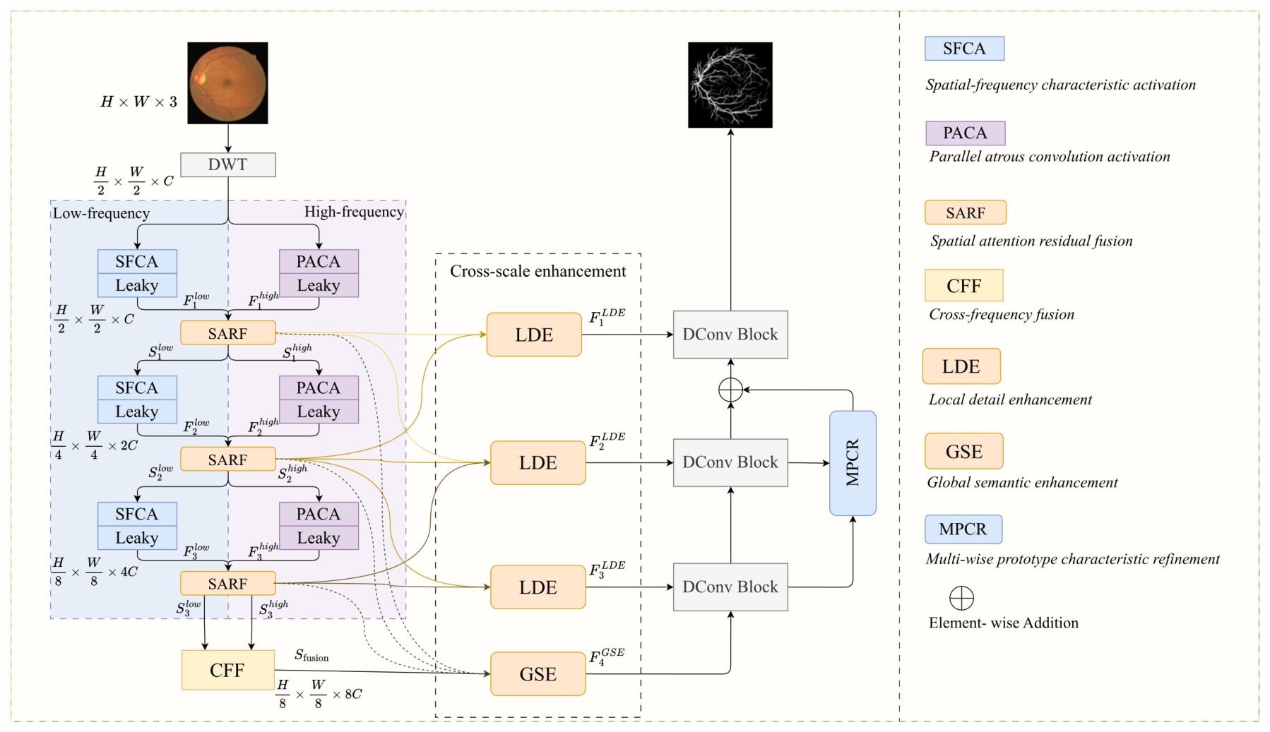
In our approach, FDPR-DBNet jointly extracted long-range continuity information and local structural details through the SFCA, PACA, and GSE modules. Simultaneously, it aligned contextual features across diverse scales, enabled cross-scale feature interaction, and enhanced semantic consistency by constructing LDE and MPCR components, preserving structural and boundary integrity in feature representations. Overall, synthesizing these modules within a U-shaped framework coupled with a connectivity loss effectively addressed multiple challenges associated with the aforementioned methods and made the framework highly suitable for preserving continuity in elongated vessel structures.

2.2. Frequency-Domain Feature Learning

Relying solely on spatial-domain characteristics may be inadequate for effectively resolving vessel crossovers, distinguishing subtle vessel-background contrasts, and preserving vascular topology. In contrast, recent studies have reported that integrating frequency-domain analysis can help identify distinctive structural patterns in different spectral ranges. For example, FCANet [37] recast channel attention as a compression problem and integrated frequency transformation into channel attention blocks to optimize feature extraction. Moreover, GFNet [38] learned the interactions among spatial features directly in the frequency domain using learnable global filters to strengthen its capability in modeling long-distance spatial dependencies. Similarly, GLFNet [10] replaced the self-attention layer in the Transformer architecture with a global-local filter block to accelerate feature extraction. Moreover, XNet [39] applied the wavelet transform to generate low- and high-frequency sub-bands to alleviate learning biases from artificial perturbations, yet failed to consider their interactions. In addition, FAMNet [40] proposed a frequency-aware matching unit to focus on resilient, domain-agnostic frequency bands, thereby mitigating the adverse influences of both intra-domain and inter-domain variations. Nevertheless, relying solely on frequency-domain features often results in the loss of vital spatial information. In this case, FDFUNet [41] introduced a multi-scale frequency-domain filter that combined features from the frequency and spatial domains to facilitate the simultaneous extraction of global and local representations across all channels. FABRF-Net [42] integrated a Haar wavelet decomposition module with a boundary-region fusion module to facilitate cross-stream feature guidance. Furthermore, AFDSeg [43] designed an adaptive coupling strategy to harmonize spatial and frequency-domain characteristics derived from heterogeneous networks, thereby optimizing intricate local details alongside global contextual information. Recently, FSE-Mamba [44] integrated multi-scale axial attention frequency-spatial coordinate Mamba (MSAA) and frequency-domain-guided attention (FDGA) into Mamba to mitigate its inherent directional limitations and improve vascular discrimination. More closely related to our work, FreqUNet [45] decomposed the input image into high- and low-frequency components using the discrete wavelet transform (DWT) and processed them individually to strengthen the model’s capability to perceive comprehensive feature representations across multiple spectra. MSCR-Net [46] proposed a multi-stage cascaded framework to minimize high-frequency detail loss and integrated a self-attention-driven refinement module to capture long-range vascular dependencies. In summary, although these frequency-domain methods could strengthen feature extraction to some extent, they commonly fell short in modeling the intricate correlations among different frequency components and exhibited compromised inter-frequency discriminability, potentially restricting their ability to use spectral information to represent broader structural patterns and fine-grained details. The inherent single-peaked distribution of frequency characteristics, together with the multi-scale nature of spatial features, further complicated their alignment. To address these issues, we constructed a dual-branch framework consisting of both high-frequency and low-frequency pathways adhering to a frequency-domain-based DWT decomposition strategy, which were mapped into the boundary and region streams, respectively. The former branch introduced a PACA module to enhance sensitivity to critical vascular high-frequency detailed edge features and reduce the interference of noise patterns, whereas the latter integrated an SFCA module to model long-distance correlations between vessel features and preserve global feature representations. Additionally, we incorporated the SARF and CFF modules between the two branches to promote both cross-frequency adaptive selection and fusion and the mutual guidance of multi-scale vessel features through dual-stream interaction, thereby enhancing comprehensive representations of retinal vessel structures across multiple spectra.
To better contextualize our work, Table 1 provides a comprehensive comparison of representative methods, highlighting the major strengths and inherent weaknesses of each category.

3. Methodology

In this section, we describe the implementation of FDPR-DBNet. The core architecture comprises a dual-branch encoding network with frequency decomposition and a cross-scale enhancement network, which optimize cross-frequency and cross-scale feature modeling to increase sensitivity to nuanced local details and improve the parsing of complex retinal vessel semantics. These designs were built upon the following key components: spatial-frequency characteristic activation (SFCA), parallel atrous convolution activation (PACA), spatial attention residual fusion (SARF), cross-frequency fusion (CFF), cross-scale enhancement (CSE) unit combining global semantic enhancement (GSE) with local detail enhancement (LDE), multi-wise prototype characteristic refinement (MPCR), and connectivity loss function.

3.1. Network Architecture

The overall framework of the proposed FDPR-DBNet is illustrated in Figure 1, and primarily consists of a dual-branch encoder with frequency decomposition, a cross-scale enhancement middle layer, and a prototype refinement decoder. Concretely, given an input image I R H × W × 3 , it was initially decomposed into low-frequency and high-frequency spatial components through the discrete wavelet transform (DWT), with separate 1 × 1 convolutional layers applied to each component as linear projections to unify their channel dimensions. The decomposed components were processed by two parallel multi-stage hierarchical branches, generating multi-level low-frequency regional feature maps F i l o w , i { 1 , 2 , 3 } , containing rich semantic information about retinal vessel trunks, and high-frequency boundary feature maps F i h i g h containing enhanced vascular boundary details. Throughout the entire encoding stage, the SARF module enabled dual-stream adaptive selection, fusion, and mutual guidance of boundary and region characteristics at different scales using frequency awareness, and modeled inter-band dependencies, yielding feature maps S i l o w and S i h i g h at three consecutive stages of the encoder. At the bottleneck of the network, the CFF block integrated high-level semantic information from the two encoder branches to form a powerful encoding representation S f u s i o n . Subsequently, the deep feature map produced by the CFF block was processed by GSE to further enhance the perception of global context in vessel regions, producing the enhanced features F 4 G S E . In tandem, the output features produced by SARF were provided to the LDE modules to reduce feature redundancy and refine critical boundary cues through progressive cross-scale fusion, resulting in the refined features F i L D E . Following this, these enhanced features were then propagated to the corresponding prototype-refinement decoder stages to compensate for the spatial information lost through repeated downsampling in the encoder. In each decoder stage, DConv blocks cascading upsampling, concatenation, and multiple convolution layers were utilized to gradually recover the resolution of the feature map. At this juncture, we placed the MPCR module in the decoder to take advantage of the prototype features for efficient recalibration and alignment of ambiguous regions, refining the segmentation results. Lastly, a 1 × 1 convolutional layer was applied to generate the pixel-wise retinal vascular prediction map P. The overall workflow is outlined in Algorithm 1, where ⊕ denotes the element-wise addition.

3.2. Discrete Wavelet Transform

In our study, we used the discrete wavelet transform (DWT) to decompose the input image into different frequency components, which reduced the spatial resolution by half without any loss of information. The choice of the DWT over the discrete cosine transform (DCT) and learnable frequency transforms was guided by several critical design considerations tailored to our task: (1) While DCT was highly effective for global frequency energy compaction, it lacked the capability for simultaneous multi-scale spatial and frequency localization. In the retinal vessel segmentation task requiring precise boundaries or fine-grained structural preservation, losing spatial localization could result in segmentation performance degradation. In contrast, DWT provided excellent multi-resolution analysis (MRA), decomposing the image into specific sub-bands (LL, LH, HL, HH) that explicitly preserved both directional high-frequency details and structural spatial positions. (2) Although learnable frequency transforms offered high flexibility, they introduced a substantial number of trainable parameters, leading to higher computational overhead and a potential risk of overfitting. Instead, DWT introduced zero additional training parameters and acted as a strong, mathematically rigorous inductive bias. Taken together, whereas traditional DCT discards precise spatial localization and fully data-driven learnable frequency transforms substantially increase the number of parameters, DWT provides a parameter-free multi-resolution inductive bias that effectively balances spatial localization and frequency separation.
Algorithm 1  FDPR-DBNet Workflow
Require: 
I R H × W × 3
Ensure: 
P R H × W × 1
1:
( I l o w , I h i g h ) DWT ( I )                                ▹Frequency Decomposition
2:
for  i = 1 , 2 , 3   do
3:
    if  i = 1  then
4:
          F i l o w SFCA ( I l o w ) ; F i h i g h PACA ( I h i g h )
5:
    else
6:
          F i l o w SFCA ( S i 1 l o w ) ; F i h i g h PACA ( S i 1 h i g h )
7:
    end if
8:
     S i l o w , S i h i g h SARF ( F i l o w , F i h i g h )
9:
end for
10:
S f u s i o n CFF ( S 3 l o w , S 3 h i g h )                              ▹Dual-Branch Encoder Stage
11:
F 4 G S E GSE ( S 1 l o w , S 2 l o w , S 3 l o w , S f u s i o n )
12:
F 1 L D E LDE ( S 1 l o w , S 2 l o w ) ; F 2 L D E LDE ( S 1 l o w , S 2 l o w , S 3 l o w ) ; F 3 L D E LDE ( S 2 l o w , S 3 l o w )              ▹Skip connection
13:
D 3 DConvBlock ( F 3 L D E , F 4 G S E )
14:
D 2 DConvBlock ( F 2 L D E , UpSample ( D 3 ) )
15:
D 1 DConvBlock ( F 1 L D E , UpSample ( D 2 ( MPCR ( D 3 , D 2 ) ) ) )            ▹Decoder and Prototype Refinement
16:
P Conv 1 × 1 ( D 1 )
17:
return P                                         ▹Final Prediction

3.3. Spatial-Frequency Characteristic Activation (SFCA)

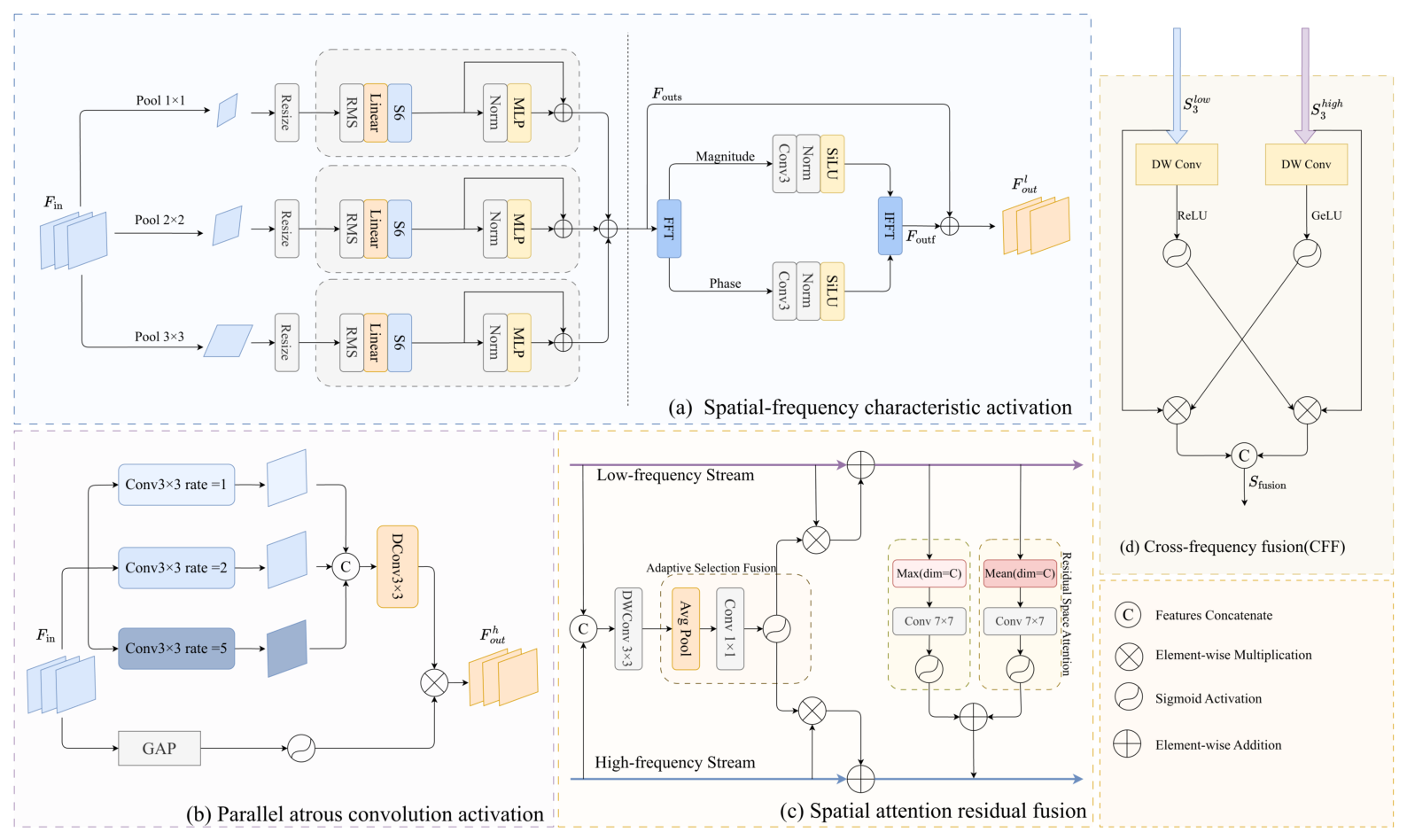
In the low-frequency branch, the SFCA block was responsible for extracting global spatial contextual representations of vessel trunk regions within low-frequency components by cascading the spatial-domain characteristic capture stage with the frequency-domain characteristic activation stage, as schematically illustrated in Figure 2a. During the spatial-domain characteristic capture phase, given an input feature map F i n R H i × W i × C i , i { 1 , 2 , 3 } , we first adopted three pooling layers to generate multi-scale feature maps, which were then flattened into sequences and passed through an efficient SSM module to extract long-range spatial feature dependencies. Within the efficient SSM block, we drew inspiration from the Vision Transformer (ViT) and substituted its self-attention component with the S6 mechanism, while applying RMSNorm for enhanced layer normalization. Ultimately, we performed an upsampling operation on the feature sequences yielded by the efficient SSM modules before fusing them to obtain the output F o u t s . During the frequency-domain characteristic activation phase, we took the output F o u t s as its input signal. Initially, we applied the fast Fourier transform (FFT) to transform F o u t s R H i × W i × C i from the spatial domain into the frequency domain and calculate the corresponding amplitude and phase spectra, as follows:
F ( u , v ) = x = 0 M 1 y = 0 N 1 f ( x , y ) e j 2 π ( u x H + v y W )
| A ( u , v ) | = R e [ F ( u , v ) ] 2 + I m [ F ( u , v ) ] 2
ϕ ( u , v ) = arctan I m [ F ( u , v ) ] R e [ F ( u , v ) ]
Herein, the variables x and y denote the spatial-domain coordinates, u and v represent frequency-domain coordinates, j is the imaginary unit, and Re and Im correspond to the real and imaginary components of F ( u , v ) , respectively. Subsequently, convolution operations were performed independently on the amplitude and phase spectra to emphasize salient regions and enhance the model’s understanding of vascular structures. Finally, the enhanced frequency-domain signal was projected back into the spatial domain via the inverse Fourier transform (IFT), followed by a residual connection to combine it with the initial input signal, resulting in the optimized low-frequency vascular feature map F o u t l . The above process could be represented as follows:
f ( x , y ) = F o u t f = 1 M N u = 0 M 1 v = 0 N 1 F ( u , v ) e j 2 π ( u x H + v y W )
F o u t l = F o u t s + F o u t f

3.4. Parallel Atrous Convolution Activation (PACA)

In the high-frequency branch, the PACA unit captured multi-scale local details related to vascular structures and boundaries within the high-frequency components using a cascaded pyramid scheme comprising a main pathway and an auxiliary pathway, as shown in Figure 2b. The main pathway applied three parallel 3 × 3 convolutions with varying dilation rates ( r = 1 , 2 , and 5 ) to the input feature map F i n , establishing distinct receptive fields to capture multi-scale local vascular details. To extract channel-specific patterns without disrupting the underlying channel information, a channel separation strategy was utilized across all convolutions. The resulting feature maps were then concatenated along the channel dimension and subjected to a deformable convolution (DConv) operation to further refine vascular boundary cues, ultimately yielding the output F m a i n of the main pathway. Concurrently, the auxiliary pathway performed a channel attention operation to model channel-wise interdependencies and activate prominent signals while attenuating redundant information, thereby constructing the channel attention weight map ω a u x . Finally, we performed tensor-level multiplication between F m a i n and ω a u x to obtain the refined, high-frequency salient output F o u t h of the PACA module. The whole computation process could be outlined as follows:
F m a i n = A C o n v r = 1 ( F i n ) + A C o n v r = 2 ( F i n ) + A C o n v r = 5 ( F i n )
ω a u x = σ ( C o n v 1 × 1 ( M e a n ( F i n ) ) )
F o u t h = D C o n v ( F m a i n ) ω a u x
where σ denotes the Sigmoid function, M e a n ( · ) represents the global average pooling operation, ⊗ denotes element-wise multiplication, and A C o n v and D C o n v refer to atrous convolution and deformable convolution, respectively.

3.5. Spatial Attention Residual Fusion (SARF)

In the dual-branch encoder, the high-frequency branch (boundary stream) contained high-resolution vascular texture and fine boundary cues, whereas the low-frequency branch (region stream) primarily captured low-resolution deep semantic features relevant to vascular backbone regions. To fortify cross-level feature alignment and exchange between them, we developed a SARF module to achieve adaptive selection and fusion as well as mutual guidance of region and edge features at different scales, as depicted in Figure 2c. This module was characterized by two core functions: (1) adaptive selection interaction and fusion, which optimized area and edge feature representations via dual-stream interaction, and (2) edge residual guidance, which injected precise edge cues into the regional context for fostering complementary feature expression.
To be concrete, we first concatenated the input features F i h i g h , i { 1 , 2 , 3 } and F i l o w from the high- and low-frequency branches and then processed the concatenated features using a 3 × 3 depthwise convolution (DWConv) to obtain the fused feature map F i k . Following that, channel-wise average pooling was applied to F i k , followed by a 1 × 1 convolution and sigmoid activation to obtain the spatial attention weight map β i , thereby constructing a spatial selection strategy. It should be noted that the attention map acted as a learnable soft-selection mask for promoting characteristic refinement. These adaptive weights were applied to the original boundary and region streams through element-wise multiplication, respectively. Finally, we derived refined area features F i l o w and edge characteristics F i h i g h with the aid of residual connections. The specific execution process of adaptive selection interaction and fusion could be represented as follows:
β i = σ ( C o n v 1 × 1 ( M e a n ( D W C o n v 3 × 3 ( C a t ( F i h i g h , F i l o w ) ) ) ) )
F ^ i h i g h = F i h i g h β i F i h i g h , F ^ i l o w = F i l o w ( 1 β i ) F i l o w
where ⊕ denotes element-wise addition, and C a t denotes the concatenation operation.
Next, we computed the global maximum and average values of the optimized edge features along the channel dimension C, which were then sequentially fed into a 7 × 7 convolution and a sigmoid activation function to generate the spatial attention maps. These two spatial attention maps were integrated via element-wise addition to yield the fused attention map M i . Subsequently, element-wise multiplication and a 3 × 3 convolution were applied to propagate refined edge cues into the area stream, thereby providing boundary residual guidance. The specific execution process of boundary residual guidance could be expressed as follows:
M i = σ ( C o n v 7 × 7 ( M a x ( F ^ i h i g h ) ) ) + σ ( C o n v 7 × 7 ( M e a n ( F ^ i h i g h ) ) )
S i l o w = C o n v 3 × 3 ( F ^ i l o w M i ) , S i h i g h = C o n v 3 × 3 ( F ^ i h i g h )
where S i l o w and S i h i g h indicate refined blood vessel region and boundary features produced under the guidance of the SARF module, respectively.

3.6. Cross-Frequency Fusion (CFF)

Simple concatenation or weighted fusion without specific consideration of the feature content across different frequency bands may incur unwanted nonlinear interactions and compromised inter-frequency discriminability. In this context, we introduced a simple yet effective CFF unit as a supplement to the SARF module and strategically placed it at the end of the dual-branch encoder to learn a more comprehensive feature representation from multiple spectral components. Its structure is shown in Figure 2d. In particular, the feature maps S 3 l o w and S 3 h i g h from the dual-branch encoder were passed through a depthwise separable convolutional layer and activated by their corresponding activation functions (ReLU and GELU) to generate the weighted spatial attention maps W l o w and W h i g h , respectively. Afterwards, we performed a cross-branch element-wise multiplication between the original inputs and their corresponding attention maps, and concatenated them to obtain the fused feature map S f u s i o n . Through the CFF unit, the interaction strength between the encoder branches could be adaptively regulated, which encouraged the network to learn more comprehensive feature representations from multiple frequency bands. The above execution process of the CFF unit could be summarized by the following equations.
W l o w = σ ( R e L U ( D W C o n v 3 × 3 ( S 3 l o w ) ) )
W h i g h = σ ( G E L U ( D W C o n v 3 × 3 ( S 3 h i g h ) ) )
S f u s i o n = C a t ( ( W l o w W h i g h ) , ( W h i g h W l o w ) )
where G E L U and R e L U indicate the GELU and ReLU activation functions.

3.7. Cross-Scale Enhancement (CSE)

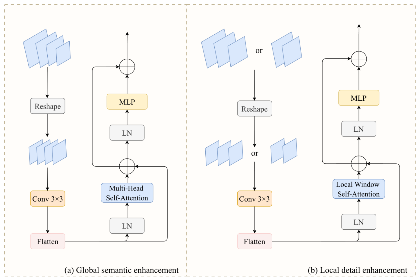
Considering that insufficient integration between local fine-grained boundary details and global contextual structure semantics relative to retinal blood vessels may lead to fuzzy boundaries and inaccurate segmentations, we meticulously constructed a CSE unit between the encoder and decoder that contained a global semantic enhancement (GSE) module and a local detail enhancement (LDE) block. Both GSE and LDE blocks took the feature pyramid from the dual-branch encoder as inputs and introduced local window self-attention and global self-attention mechanisms to progressively fuse local and global contextual feature information for reducing semantic shifts across adjacent levels and enhancing feature representations, which encouraged the model to adapt to variations in vessel structures. As depicted in Figure 3a, the GSE module received a four-level global feature pyramid F = { S 1 l o w , S 2 l o w , S 3 l o w , S f u s i o n } derived from the dual-branch encoder, and utilized a spatial resizing operation to resize them to a predefined target size. Subsequently, these multi-scale feature maps were fused using a 3 × 3 convolution, followed by a flattening operation to obtain the sequence F . Eventually, these flattened feature maps were provided to a Transformer block to dig out multi-scale global contexts. The specific implementation was as follows:
F = F l a t t e n ( C o n v 3 × 3 ( C a t ( R e s h a p e ( F ) ) ) )
F a = F + M H S A ( L N ( F ) )
F o = F a + M L P ( L N ( F a ) )
where M H S A represents a multi-head self-attention operation, and M L P indicates a multi-layer perceptron. Diverging from the GSE block, we replaced its self-attention component with a simple local window self-attention mechanism and used a local feature pyramid comprising the output features of adjacent stages within the dual-branch encoder as input, thereby constructing an LDE module to reduce semantic bias across scales and capture fine vascular boundary and texture cues. Depending on the placement stage of the LDE module, the local feature pyramid was configured with either two layers (for Stages 1 and 3) or three layers (for Stage 2). These pyramid features were reshaped to match the required target resolution of the corresponding stage, and then concatenated along the channel dimension. After aggregation via a 3 × 3 convolution, the fused features were forwarded to a modified Transformer for further refinement.

3.8. Multi-Wise Prototype Characteristic Refinement (MPCR)

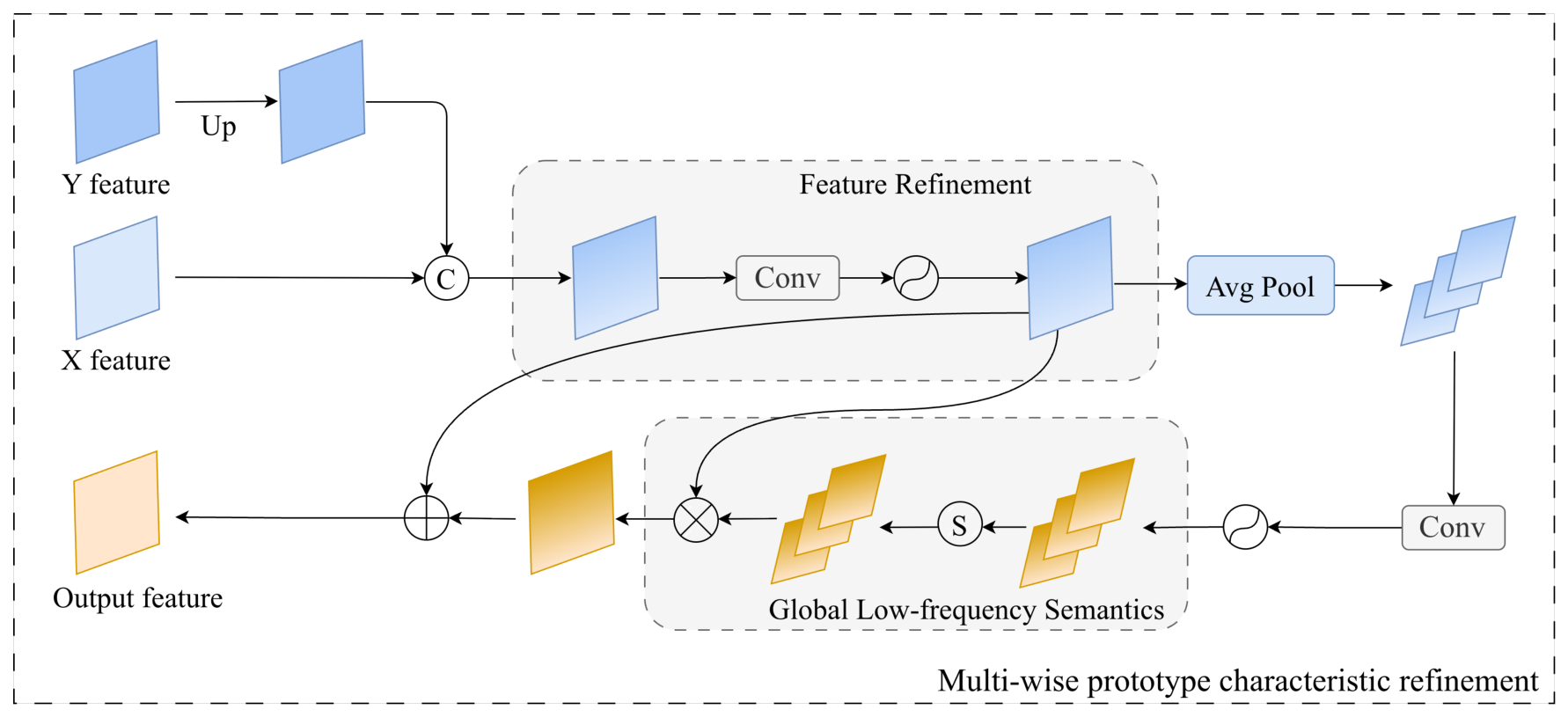
Inconsistent semantic representations in multi-scale features may cause misalignment, which can be mitigated by representing high-response features in the low-frequency domain. To address this issue, we designed an MPCR block to efficiently perceive and calibrate multi-scale feature components in the decoder using prototype features, as shown in Figure 4. The computational flow could be divided into three primary stages: (1) Feature alignment and fusion: The module received high-resolution detailed features X R H 4 × W 4 × C 4 and low-resolution semantic features Y R H 4 2 × W 4 2 × C 5 , wherein Y first underwent an upsampling operation (Up) to align its spatial dimensions with those of X before being fused with X through a concatenation operation. (2) Feature refinement: The concatenated feature map then underwent a refinement process via a 3 × 3 convolution and an activation function to yield f R H 4 × W 4 × C 4 , which served to integrate the fused information and extract a unified, robust feature representation. (3) Global low-frequency semantic interaction: First, a global average pooling operation was performed on the refined feature map f to compress the spatial dimensions and capture global contextual information into a 1D channel descriptor. Subsequently, this descriptor was processed through a 3 × 3 convolution and an activation function to generate the low-frequency prototype feature p R 1 × 1 × C 4 . The prototype feature p was subjected to a probability mapping operation to highlight salient low-frequency components, resulting in p 1 R H 4 × W 4 × C 4 . Subsequently, we performed element-wise multiplication between f and p 1 to probe cross-scale semantic consistency and obtain a refined representation p 2 R H 4 × W 4 × C 4 . Lastly, we integrated p 2 and f using an element-wise addition operation. The mathematical formulation of the aforementioned three stages could be summarized as follows:
f = R e L U ( C o n v 3 × 3 ( C a t ( X , U p ( Y ) ) , a x i s = 1 ) )
p = R e L U ( C o n v 3 × 3 ( M e a n ( f ) ) )
p 1 ( i , j , c ) = σ ( p ( i , j , c ) ) = 1 1 + e p ( i , j , c )
p 2 ( i , j , c ) = f ( i , j , c ) p 1 ( i , j , c )
F o u t ( i , j , c ) = p 2 ( i , j , c ) f ( i , j , c )
where i and j denote the spatial coordinates of the feature map f, and c denotes feature category information. Through the dynamic feature calibration mechanism within the designed MPCR block, cross-scale semantic shifts were precisely aligned, and vascular boundary integrity within feature representations was effectively preserved and enhanced.

3.9. Connectivity Loss Function

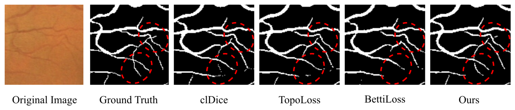
Guided by the prior knowledge that an ideal prediction of vascular structures should minimize fragmented components and maintain topological continuity and integrity, we formulated a connectivity loss function, L C , designed to incentivize the model to prioritize continuous and coherent vascular structures. This loss, L C , measured the degree of connectivity and penalized vessel discontinuities in the prediction by comparing the number of connected components between the predicted segmentation Y and the ground truth Y G , as follows:
L C = | # c ( Y ) # c ( Y G ) | # ( Y G )
In this equation, # c ( Y ) and # c ( Y G ) denote the number of connected components in Y and Y G , respectively, and # ( Y G ) indicates the number of pixels in Y G . In particular, we introduced a smoothness penalty S ( Y ) to calculate spatial pixel differences, which provided an approximation of the number of undifferentiated connected components to evaluate vascular connectivity. The smoothness penalty S ( Y ) could be formulated as follows:
S ( Y ) = 1 N i , j | Y ( i , j ) Y ( i , j + 1 ) | + i , j | Y ( i , j ) Y ( i + 1 , j ) |
Here, Y ( i , j ) represents the pixel value at position ( i , j ) in Y, and N corresponds to the total number of pixels and acts as a normalization coefficient to ensure that the penalty is scale-invariant. These two terms in the formula compute spatial differences between neighboring pixels in the horizontal and vertical directions, respectively. Following the same procedure, S ( Y G ) can be derived for Y G .
In addition, we also drew upon the binary cross-entropy (BCE) loss function L B C E to prevent over-segmentation by calculating classification errors pixel by pixel. Accordingly, the overall objective loss function L T could be expressed as the combination of L B C E and L C to optimize model training, which could be given as follows:
L T = L B C E + λ L C
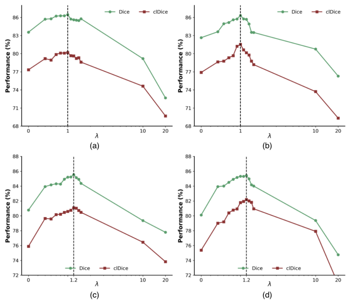
where λ denotes the balancing factor that was empirically set to 1.

4. Experiments

4.1. Datasets

To ensure an objective evaluation of the segmentation performance of the developed model in this study, we utilized four well-recognized retinal datasets: DRIVE, CHASE_DB1, STARE, and IOSTAR. At the same time, we followed the data partitioning protocol described in prior work [47,48,49,50] to ensure a fair and consistent comparison with existing benchmarks. A detailed summary of these datasets is provided in Table 2.

4.2. Evaluation Metrics

In this study, we adopted widely acknowledged metrics to comprehensively evaluate the model’s segmentation performance across the datasets, namely sensitivity (SE), specificity (SP), accuracy (ACC), precision (PR), Dice score (Dice), and the Matthews correlation coefficient (MCC). These indicators were computed according to the confusion matrix, defined as follows:
S E = T P T P + F N
S P = T N T N + F P
A C C = T P + T N T P + T N + F P + F N
P R = T P T P + F P
D i c e = 2 × T P F P + F N + 2 × T P
M C C = T P × T N F P × F N ( T P + F P ) ( T P + F N ) ( T N + F P ) ( T N + F N )
Among these equations, true positives (TP) and true negatives (TN) indicate correctly predicted vascular and non-vascular pixels, respectively, while false positives (FP) and false negatives (FN) represent their incorrectly predicted counterparts. In addition, we also employed the area under the curve (AUC) for both the precision–recall (PR) curve and the receiver operating characteristic (ROC) curve to quantitatively analyze the performance of the vessel segmentation task. Additionally, centerline Dice (clDice) [51] was incorporated to specifically quantify the topological connectivity and continuity of the vascular network based on centerline skeleton extraction. For these metrics, a value closer to 1 signified better segmentation results. Notably, we conducted five independent runs using different random initializations and reported the average results to guarantee the robustness and reliability of our findings. These indices were expressed as percentages (%), with values ranging between 0% and 100%.

4.3. Implementation Details

Our network was implemented in Python 3.10 and PyTorch 2.0 on an Ubuntu 20.04 workstation equipped with two NVIDIA GeForce RTX 4070 Ti GPUs, each featuring 12 GB of VRAM. During training, we uniformly resized all images to a resolution of 512 × 512 and employed the Adam optimizer with a CosineAnnealingLR schedule to dynamically adjust the model’s parameters, with both the initial learning rate and the weight decay rate set to 10 4 . For the loss function, the weight balancing parameter λ was set to 1. Furthermore, data augmentation techniques, such as Contrast Limited Adaptive Histogram Equalization (CLAHE), were also applied to mitigate overfitting. The model was trained for a maximum of 100 epochs with a batch size of 8 on each dataset. Notably, no post-processing was performed after segmentation. The specifications of our experimental settings and the detailed parameter configurations for each network component of the proposed FDPR-DBNet are listed in Table 3.
For the local detail enhancement (LDE) block, the localized window size was configured to M × M with a sliding stride of M, where M = 8 in our experiment. To establish cross-window connections, a shifted-window partitioning approach was applied with a shift of M / 2 . To ensure full coverage of the entire image by the sliding windows, regardless of the input dimensions, an adaptive padding strategy was implemented. The padding width was dynamically calculated as ( 8 D mod 8 ) , where D represents the original dimension size. In each LDE unit, the number of input channels (C) and attention heads (N) within the multi-head self-attention (MSA) were uniformly fixed as 128 and M / 2 , respectively, thereby keeping the per-head projection dimension invariant at d = C N = 32 . Beyond that, the MLP expansion ratio was uniformly set to M / 4 . The global semantic enhancement (GSE) block applied a self-attention mechanism to model global long-range dependencies across the whole vascular tree. Following the configuration of LDE, this module also utilized 4 attention heads and a per-head dimension of 32, while assigning an MLP expansion ratio of 2.

4.4. Comparisons with the State-of-the-Art Methods

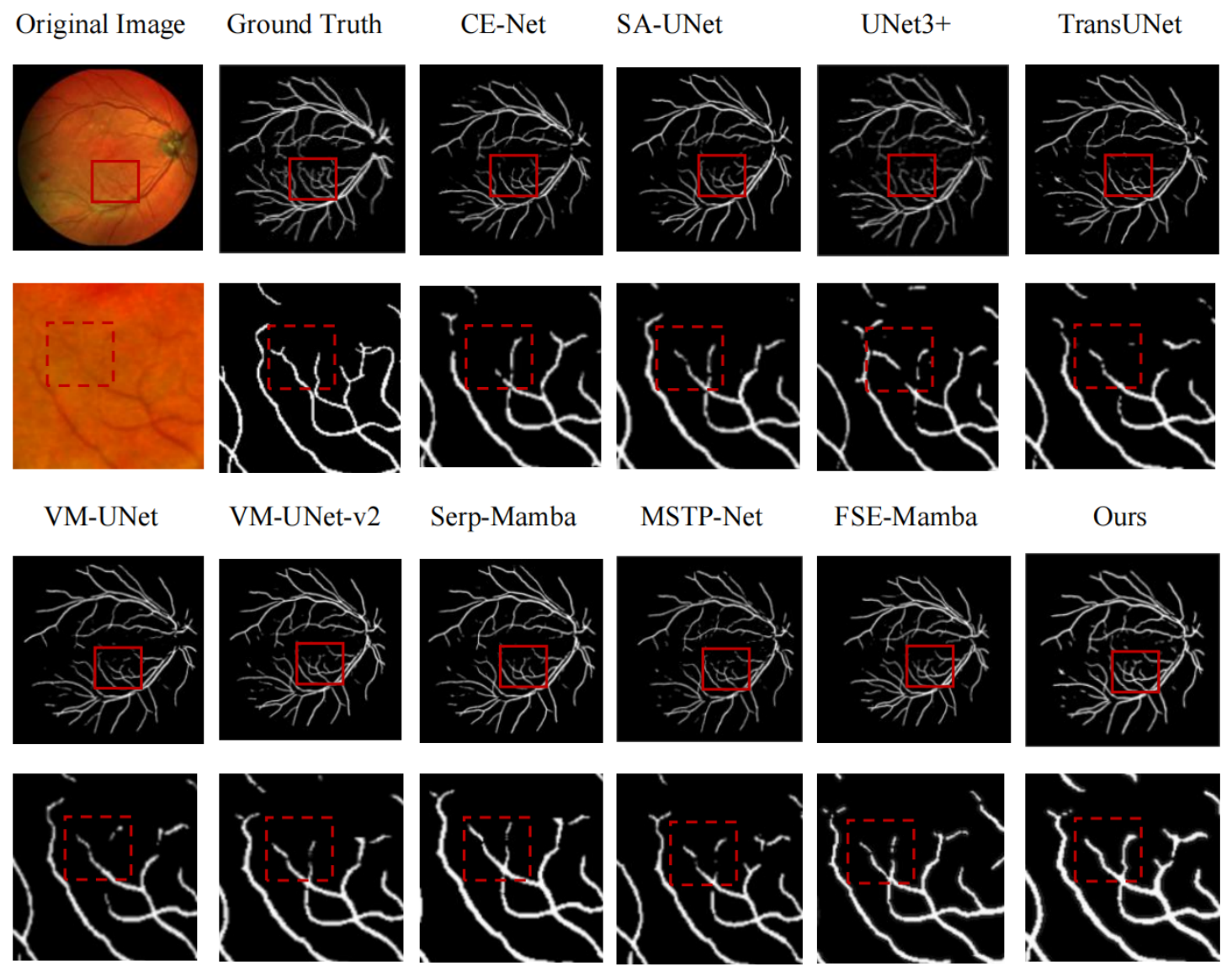
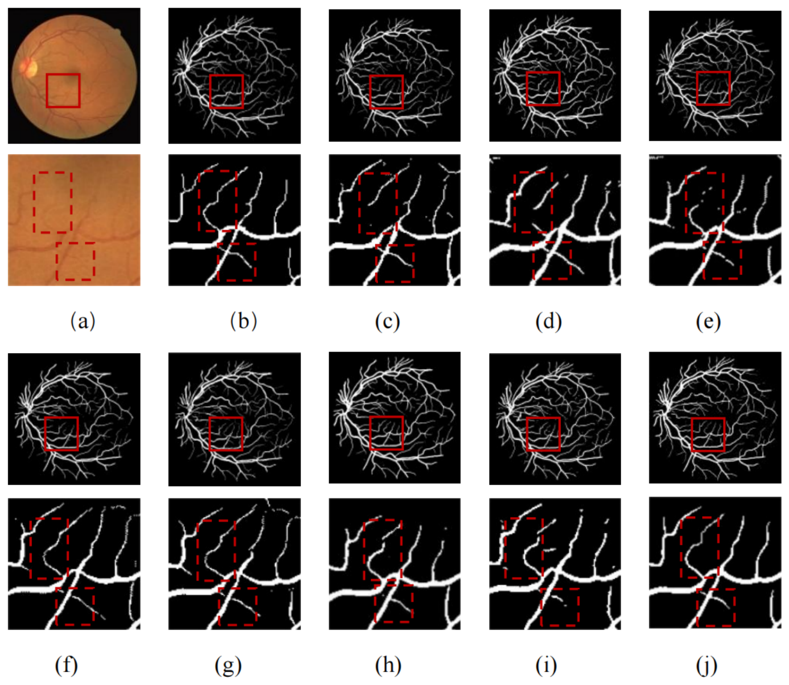
We conducted a comprehensive and holistic comparison analysis between our FDPR-DBNet and a range of current state-of-the-art methods on the DRIVE, CHASE_DB1, and STARE datasets. These methods mainly involved several representative general medical image segmentation models (including U-Net [8], CE-Net [15], LadderNet [14], U-Net3+ [16], TransUNet [21], VM-UNet [31], and VM-UNet-v2 [32]), and models specifically designed for retinal vessel segmentation (containing SA-UNet [17], MSTP-Net [19], PA-Net [24], Serp-Mamba [33], and CRMA-UNet [34]). We also embraced comparisons with two advanced frequency-domain-based segmentation methods, comprising FreqUNet [45] and FSE-Mamba [44]. Except for data for PA-Net, FreqUNet, MSCR-Net, SDHM2T, and CRMA-UNet, which were cited directly from the original papers, the results for the remaining methods were obtained experimentally using the released source code and the default parameter configurations provided in their literature. The comparison results are summarized in Table 4, Table 5 and Table 6, where “–” denotes unavailable data, while boldface and underlined text indicate optimal and second-ranked results, respectively. It is evident from the data in Table 4, Table 5 and Table 6 that the proposed FDPR-DBNet demonstrated superior segmentation performance across most evaluation metrics. To support the quantitative data, we also provide an intuitive visual comparison of segmentation results between our model and other cutting-edge methods in Figure 5, Figure 6 and Figure 7 on these datasets.
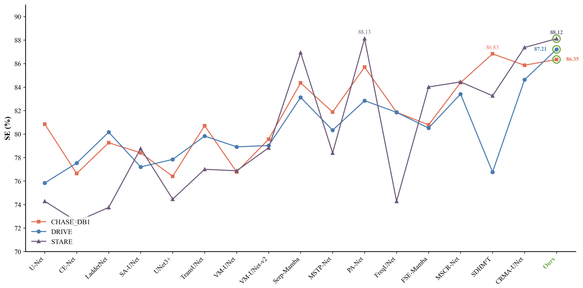
Quantitative analysis: Initially, in terms of the sensitivity (SE) indicator, Our FDPR-DBNet established new state-of-the-art performance on the DRIVE dataset, reaching a top SE score of 87.21%, an improvement of 2.59% over the second-best-performing method, CRMA-UNet. On the CHASE_DB1 and STARE datasets, it achieved sub-optimal performance, with competitive scores of 86.35% and 88.12%, respectively, nearly approaching the scores of the top-performing SDHM2T and PA-Net. The SE metric reflected its capability in segmenting vessel target regions, where a higher SE score directly correlated with a reduction in the incidence of missing vessel pixels. This could be further confirmed by qualitative segmentation comparison results. As shown in Figure 5 and Figure 6, our model identified more vascular pixels when compared with other approaches. It should be emphasized that the SE indicator did not account for the misclassification of non-vessel pixels as vessels, and other indicators were required for further performance assessment.
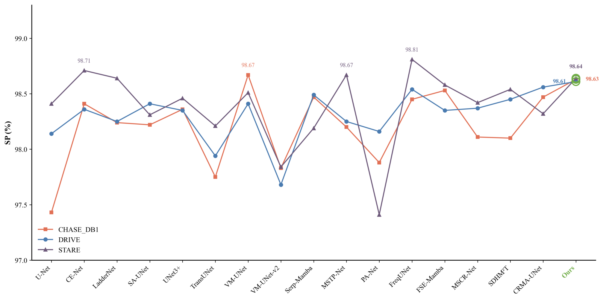
Concerning the specificity (SP) metric, our model achieved scores of 98.80%, 98.63%, and 99.02% on the DRIVE, CHASE_DB1, and STARE datasets, respectively. Its SP scores on the DRIVE and CHASE_DB1 datasets were 0.05% and 0.29% lower than those of CRMA-UNet, respectively. Nevertheless, our model outperformed CRMA-UNet on the other reported metrics for these datasets and across all reported metrics on the STARE dataset. Given that the single SP metric may ignore the omission of vascular pixels, it was necessary to combine it with the SE indicator for a more comprehensive insight into the model’s performance. As illustrated in Figure 5, Figure 6 and Figure 7, it was again confirmed that missegmentations occurred infrequently in our FDPR-DBNet, underscoring its effectiveness in discriminating target vascular pixels from non-vessel pixels.
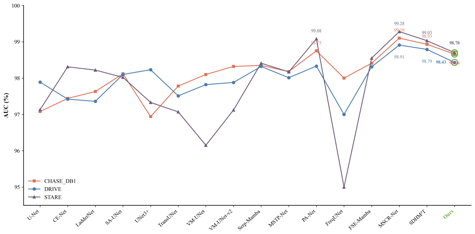
As a threshold-independent metric, the Area Under the Curve (AUC) provided a holistic evaluation of the model’s discriminative ability. On the DRIVE dataset, our model achieved an AUC score of 98.43%, outperforming other state-of-the-art methods like PA-Net (98.33%) and Serp-Mamba (98.32%). In contrast, it was narrowly surpassed only by PA-Net (98.66% vs. 98.75%, and 98.70% vs. 99.08%) on the CHASE_DB1 and STARE datasets, and maintained a clear advantage by 0.31% and 0.29% over Serp-Mamba. In conclusion, the AUC range of 98.43% to 98.70% achieved by our model across diverse datasets demonstrated its exceptional robustness in distinguishing vascular pixels, underscoring its state-of-the-art performance in current retinal vessel segmentation tasks.
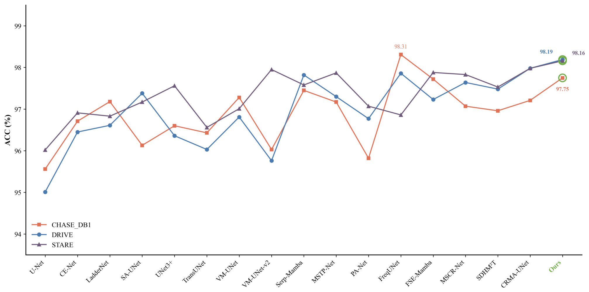
In the case of Accuracy (ACC), our model performed best on the CHASE_DB1 and STARE benchmarks, leading the second-best-performing CRMA-UNet by approximately 0.21% and 0.18%, respectively. On the DRIVE dataset, our model scored 97.75% and obtained a competitive second-place ranking, which only lagged behind the top-performing FreqUNet by about 0.56%. However, in other indicators, FreqUNet was inferior to it by a large margin. Similarly, regarding the precision (PR) indicator, our model consistently maintained a substantial lead on the DRIVE and CHASE_DB1 datasets, with—at least—additional gains of 0.70% and 1.65%. Even on the STARE benchmark, our model still secured the second position, only slightly falling short of Serp-Mamba by 0.65%. These outcomes highlighted that our model demonstrated a superior capability to accurately distinguish vascular regions. Given that vascular pixels occupied only a small fraction of the image, the resulting class imbalance rendered ACC and PR insufficient metrics for evaluating overall performance. Consequently, the Dice coefficient was necessary to further assess the model’s segmentation performance.
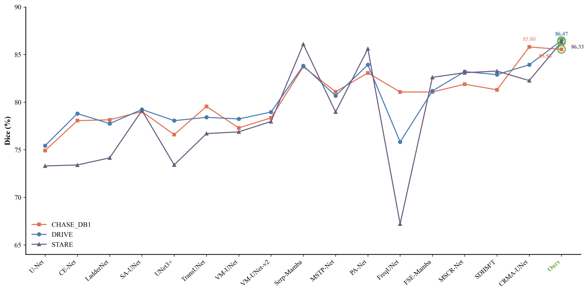
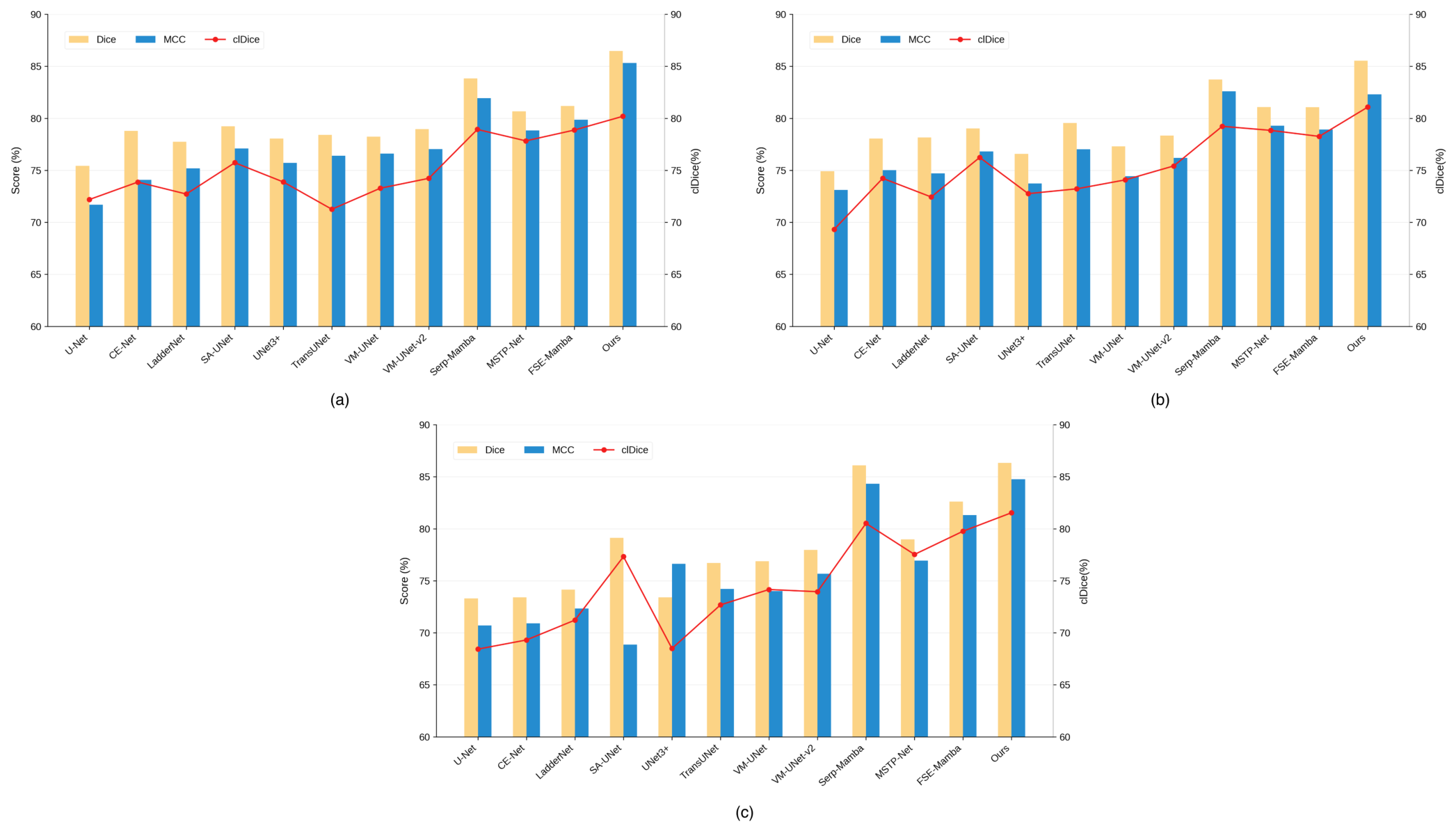
As for Dice, a harmonic mean of precision and sensitivity, our model demonstrated exceptional results at 86.47% and 86.33% on the DRIVE and STARE datasets, respectively. Specifically, it significantly outperformed the competing CRMA-UNet and PA-Net models by 2.54% on the DRIVE dataset, which demonstrated its superior capability in segmenting blood vessels both accurately and completely. At the same time, it also showed a margin gain of 0.24% over the second-best Serp-Mamba on the STARE benchmark, while building a solid advantage of 0.72% over PA-Net. Conversely, on the CHASE_DB1 dataset, it ranked second with a Dice score of 85.55% and delivered a narrow drop by only 0.25% when compared to CRMA-UNet, whereas it kept an obvious advantage over other recent models like Serp-Mamba (83.73%) and PA-Net (83.08%). Compared to MSCR-Net and SDHM2T, our model consistently maintained a highly competitive advantage, outperforming these very recent methods in Dice by 3.26% and 3.57% on the DRIVE dataset, 3.91% and 4.50% on the CHASE_DB1 dataset, as well as 3.23% and 3.06% on the STARE dataset, respectively. Of note, CRMA-UNet did not exhibit a performance superiority over our model across other assessment indicators. The consistently high Dice (ranging from 85.55% to 86.47%) substantiated that our FDPR-DBNet accurately recognized the foreground (vessels) while minimizing false positives. Our model achieved MCC scores 8.02%, 2.15%, and 2.61% higher than those of SDHM2T on the DRIVE, CHASE_DB1 and STARE datasets, respectively. While our model’s MCC score on the CHASE_DB1 dataset was marginally lower than that of Serp-Mamba by 0.28%, our model established a clear dominance in clDice, outperforming it by approximately 1.85%. These results validated our model’s superior ability to preserve vascular connections and prevent capillary fragmentation. Beyond that, we could observe from Figure 5, Figure 6 and Figure 7 that our model effectively recognized refined retinal blood vessels, further confirming our model’s benefits in precisely segmenting vascular pixels and attenuating irrelevant noise.
To further analyze performance trends across various metrics among different methods, we carried out visualizations on comparative data using line plots (See Figure 8, Figure 9, Figure 10, Figure 11, Figure 12 and Figure 13). In these plots, each data point corresponded to a specific method, with yellow markers highlighting the proposed FDPR-DBNet, which achieved top-tier scores with respect to the corresponding indicator. While the general trends indicated that numerical variances among most state-of-the-art methods were relatively narrow, our FDPR-DBNet exhibited a pronounced performance edge in ACC, SE, and AUC across most datasets. Furthermore, the model maintained a highly competitive standing in Dice, collectively sustaining the robustness and superiority of the proposed FDPR-DBNet.
By scrutinizing the experimental results for the three datasets, we found that, compared with CNN-based segmentation methods, models combining Transformers with CNNs (such as PA-Net and TransUNet) generally achieved better segmentation performance, which may be due to their ability to effectively model long-range global and local dependencies among vessel features. Moreover, Mamba-based methods like Serp-Mamba generally performed better than CNN-based and Transformer-based methods. Concretely, Mamba-based models showed consistent improvements over TransUNet (78.41%, 79.55% and 76.70%) in terms of Dice, with Serp-Mamba reaching up to 83.83%, 83.73%, and 86.09%, respectively. Other key indices also showed a similar trend on these three datasets, demonstrating a strong capacity to accurately identify complex vessel structures. These advantages of Mamba-based methods could be attributed to more effective long-distance modeling power and an efficient selective state-space layer. An interesting observation was that frequency-domain-based methods possessed a certain degree of merit over spatial domain-based ones. For example, a frequency-domain method, FSE-Mamba, offered highly competitive AUCs of 98.31%, 98.41%, and 98.55% across all three datasets, rising by around 0.30%, 0.23%, and 0.38% over the spatial-domain-based model MSTP-Net, respectively. This affirmed the benefits of integrating frequency-domain modeling to preserve and process intricate vascular structural details. Ultimately, our FDPR-DBNet, a novel frequency-domain-based method, delivered near-optimal performance gains across all three datasets and reemphasized the efficacy of integrating frequency-domain information to capture fine-grained vessel details. Compared with other recently reported frequency-domain methods like FreqUNet and FSE-Mamba, the Dice score improved by 10.65%, 8.32%, and 19.12% over FreqUNet across the three benchmarks, while increasing from 81.18% to 86.47%, 81.07% to 85.55%, and 82.61% to 86.33% compared with FSE-Mamba, respectively. Moreover, it also maintained a highly stable AUC across all datasets, ranging from 98.43% to 98.70%, whereas FreqUNet showed more volatility, dropping from a competitive 98.00% on the CHASE_DB1 dataset down to 95.00% on the STARE dataset. Meanwhile, FSE-Mamba also displayed a similar fluctuating trend. The observed performance gains originated from several synergistic modules. Theoretically, our model bypassed this via DWT, isolating fine boundary details through PACA in the high-frequency branch and macro-structures via SFCA in the low-frequency branch. Furthermore, the SARF and CFF modules enabled adaptive fusion and mutual guidance of frequency-aware region and boundary features at different scales by dual-branch interaction based on a residual self-attention mechanism, which suppressed irrelevant noisy information, learned refined boundary features, and optimized region representations. Through the CSE block, our model established an explicit mathematical trade-off between localized pixel clarity (via LDE) and long-range structural continuity (via GSE), which prevented vessel fragmentation and elevated topological continuity. The MPCR module leveraged high-order prototype alignment for dynamic feature calibration, which enabled the network to distinctively suppress non-vascular confounding artifacts and preserve structural integrity in feature representations. Beyond that, a tailored connectivity loss function that penalized fragmentation and disconnection phenomena within the predicted vascular network further guided the model to better preserve the underlying topological structure of blood vessels.
Qualitative analysis: As can be seen from the visual comparison results between our model and other advanced methods in Figure 5, Figure 6 and Figure 7, our model attained superior segmentation performance in some challenging scenarios. Traditional convolutional methods such as CE-Net and SA-UNet exhibited omissions of details at the distal branches of retinal blood vessels and suffered from significant structural disconnections or broken vessel segments in low-contrast regions of the DRIVE dataset. Even UNet3+ and TransUNet occasionally introduced noise or lost fine details. Although Mamba-based methods like VM-UNet and Serp-Mamba performed well, they still showed slight over-segmentation in dense regions. On the CHASE_DB1 dataset featuring higher resolution images, while models such as MSTP-Net and FSE-Mamba exhibited strong discriminative capacity to identify blood vessels by focusing on multi-scale features, false positives in areas with low contrast still occurred. The STARE dataset often contained pathological characteristics (like exudates), which complicated the task of vessel segmentation. These advanced models like TransUNet and Serp-Mamba tended to lose structural integrity in highly curved vessel paths and failed to maintain the topological continuity of fine-grained capillaries. Even in the presence of a frequency-guided attention mechanism, FSE-Mamba exhibited a tendency to prioritize dominant global structures, but occasionally missed the most minute terminal capillaries or showed over-smoothing at the junctions where multiple vessels crossed. It still struggled to retrieve delicate high-frequency signals, which inevitably led to the undesirable omission of fine terminal vessels. In contrast, our model predicted a relatively intact and continuous blood vessel network that aligned more closely with the ground truth, especially in the peripheral regions where vessel signals are weakest. In a nutshell, the proposed FDPR-DBNet stood out as a high-performing model that bridged the gap between global structural awareness and local fine details relevant to retinal blood vessels through the mutual coordination of SFCA, PACA, SARF, CFF, LDE, GSE, and MPCR modules. Its innovative architecture and hierarchical feature extraction strategy enabled the acquisition of more nuanced and comprehensive characteristic representations to successfully overcome the discontinuity issue that appeared in Transformer and Mamba models, effectively preserving vascular integrity and continuity.
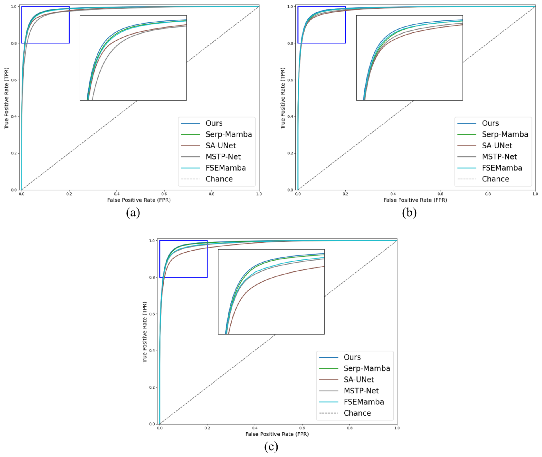
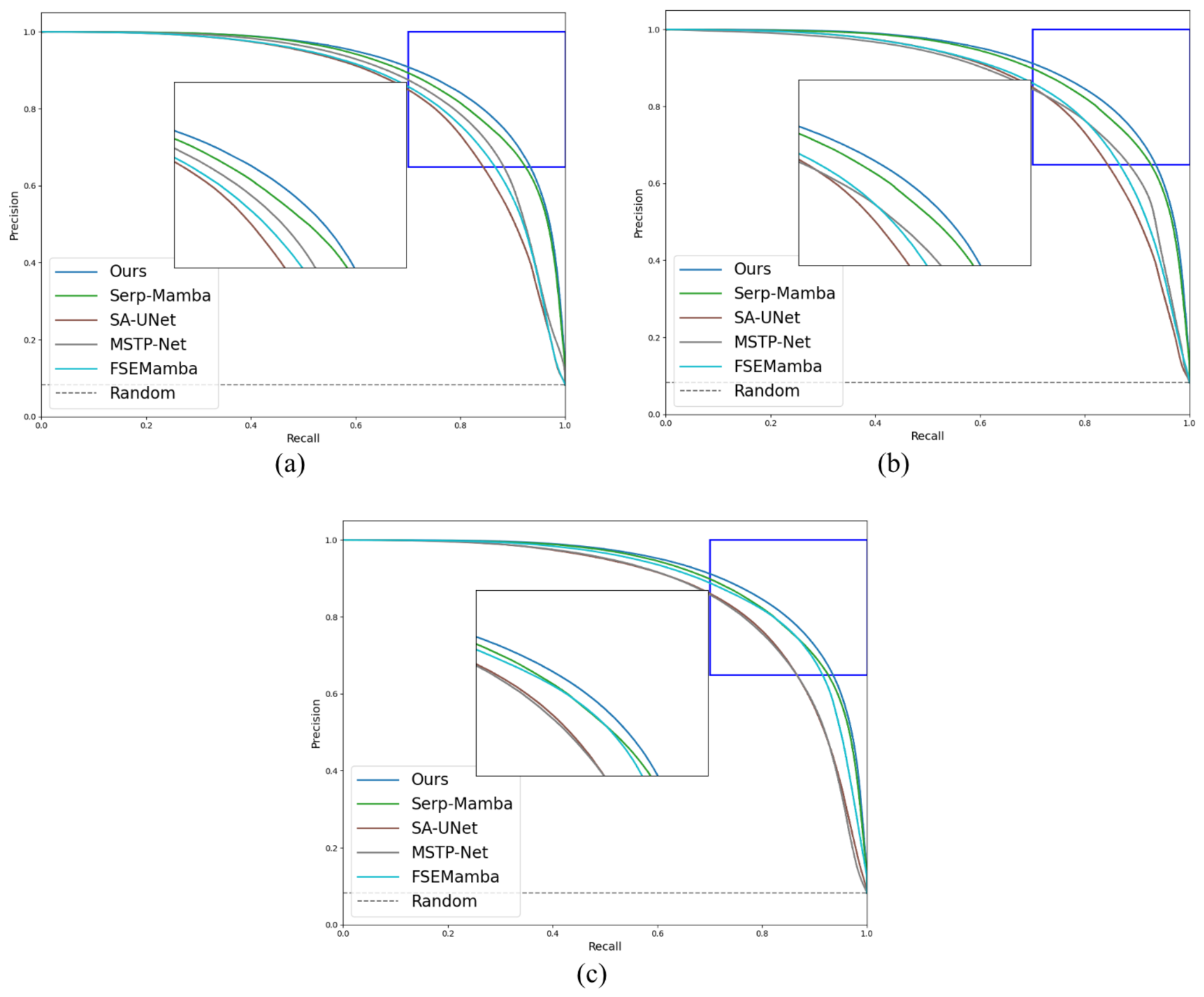
To further investigate various network performance metrics, we additionally employed the ROC and precision–recall (P-R) curves for the DRIVE, CHASE_DB1, and STARE datasets, as displayed in Figure 14 and Figure 15. The ROC curves provided a comprehensive assessment of discrimination by considering both positive and negative samples, whereas the precision–recall curves emphasized positive samples and were therefore well suited to imbalanced data. Upon observation, it was apparent that the ROC curves for our model across all three datasets consistently occupied the upper-left corner and enclosed the curves of other models, indicating that the model effectively distinguished vessel from non-vessel pixels while minimizing false alarms. Similarly, the P-R curves were nearly the outermost across these datasets, indicating a favorable trade-off between precision and recall. In summary, the proposed FDPR-DBNet consistently outperformed alternative methods in terms of both ROC and P-R curves. This dual-curve dominance suggested that our model was not only statistically robust but also practically effective for the high-precision requirements of retinal vessel segmentation.

4.5. Comparison Analysis on High-Resolution Dataset

In order to further validate the model’s segmentation performance on high-resolution images, we conducted experiments on the IOSTAR dataset, which contains 30 images with a resolution of 1024 × 1024 pixels. Using the same experimental parameters, we repeated the experiment on this dataset and compared the results with those of several state-of-the-art models. The quantitative and qualitative comparisons are presented in Table 7 and Figure 16. It was clear from Table 7 that our model performed considerably well across the majority of key metrics on the high-resolution IOSTAR benchmark, particularly in SP (98.75%), Dice (85.43%), and clDice (82.70%). Although SA-UNet and Serp-Mamba reported relatively higher ACC (98.90%) and PR (84.91%) values, respectively, they lagged significantly behind our model in other metrics, exhibiting notable differences of 9.03% and 2.54% in Dice. Except for the SE indicator, our model was also superior to the direct competitor CRMA-UNet (ACC: 97.61% vs. 97.56%, and Dice: 85.43% vs. 84.67%). These results fully demonstrated the global-local contextual modeling strength of our model and its powerful feature representation capability, thereby proving its superior robustness. In addition, we could also observe from Figure 16 that our model exhibited the highest fidelity to the ground truth, particularly in maintaining the continuity of thin and tortuous retinal vessels. It effectively avoided the vessel fragmentation issues encountered in other models, and retained more boundary details of microvessels.

4.6. Comparison Analysis on Complex Retinal Images

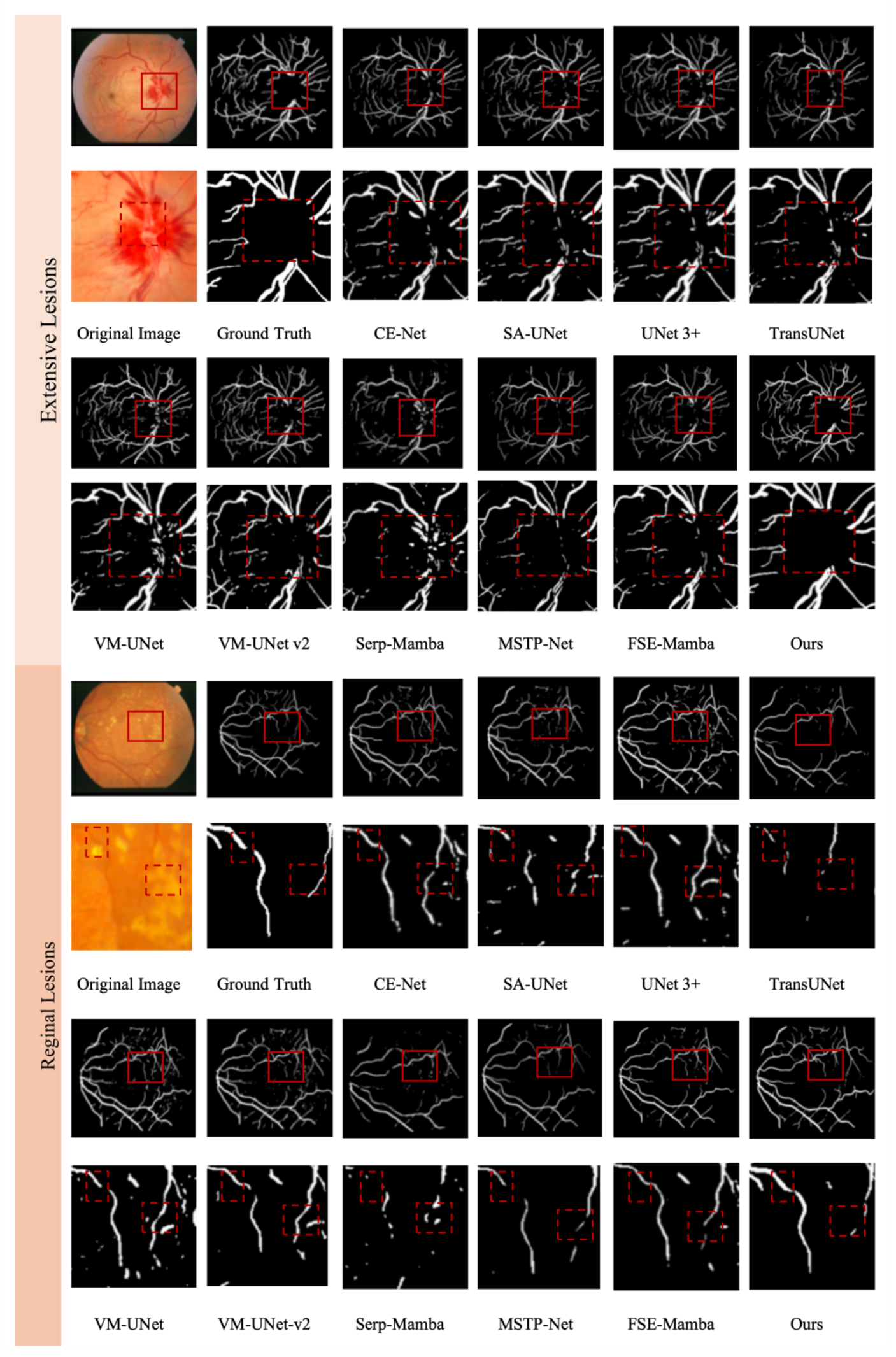
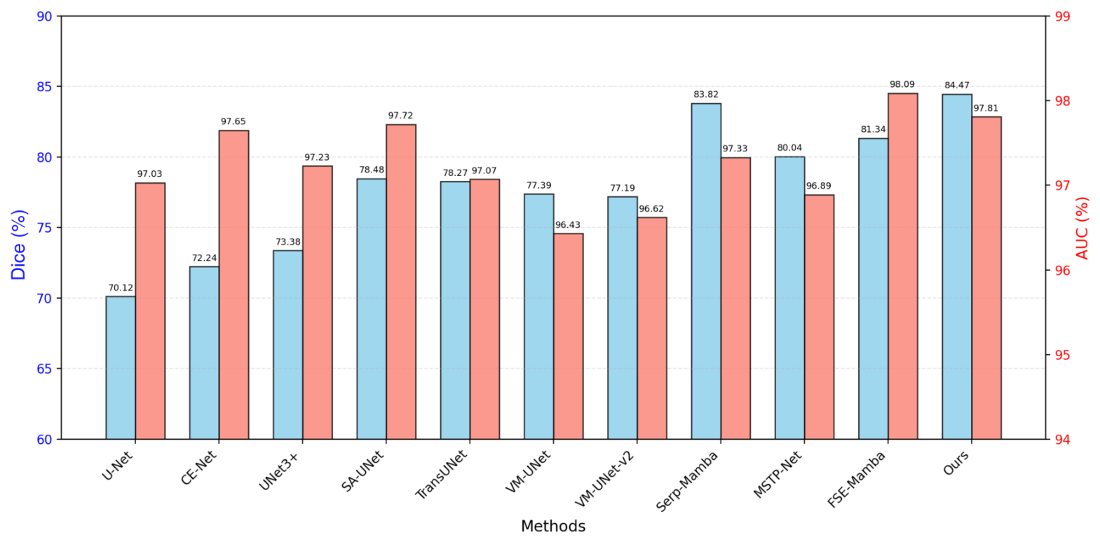
Structural alterations induced by fundus disease often exert an influence on the accuracy of retinal vessel segmentation, which may degrade segmentation performance. To assess the effectiveness of our model, we conducted segmentation testing on the ten diseased retinal images (including extensive and regional lesions) in the STARE dataset. Some samples of segmentation results across different methods are depicted in Figure 17. In addition, we also summarize the segmentation performance of several advanced methods on fundus images with extensive and regional lesions, as shown in Figure 18.
In the case of extensive lesions, the primary challenge lay in maintaining vascular structural connectivity across large and complex regions while minimizing background noise. As shown in Figure 17, traditional models like CE-Net demonstrated significant fragmentation in the segmentation of fine structures, often failing to maintain the continuity of the vessel network. While SA-UNet and UNet3+ improved smoothness, they tended to over-segment or blur boundaries. Recent Mamba-based and Transformer-based models like VM-UNet and TransUNet offered better global context awareness but still struggled with the high-frequency details required for thin and peripheral vessel segments. Our model achieved the highest fidelity to the ground truth. It effectively suppressed false positives in the presence of extensive pathological noise and preserved the integrity of the linear structures, suggesting a superior capability in capturing both long-range dependencies and local textures. In the context of regional lesions, a principal challenge required the model to distinguish subtle vessel structural changes from pathological regions in a localized context. It could be observed from Figure 17 that in localized regions, models like UNet3+ and MSTP-Net often overlooked smaller or lower-contrast vessels, leading to a loss of clinically relevant detail. Even some advanced methods such as TransUNet and VM-UNet also exhibited fuzzy boundaries and fragmentation when dealing with fine vessels around lesion regions, whilst FSE-Mamba and VM-UNet-v2 were sensitive to pathological interference and generated false-positive predictions. In contrast, although our model still incorrectly segmented a few subtle vessels in indistinct regional lesion areas, it effectively filtered out most interfering signals and produced relatively sharp and refined edges. In general, our model could minimize the influence of fundus lesions, achieve more accurate segmentation of retinal blood vessels, and preserve their topological integrity.
In Figure 18, we could clearly observe that, for diseased eye cases, our model attained remarkable segmentation performance, with the highest Dice score (84.47%) and a competitive AUC that was approximately 0.28% lower than the highest value. Its AUC score was only slightly lower than that of FSE-Mamba (less than 0.30%), whereas its Dice score was higher by a large margin of 3.13%. In this regard, the presented FDPR-DBNet confirmed clear superiority over existing advanced methods, effectively improving vessel identification accuracy in regions prone to segmentation errors. Simultaneously, its exceptional segmentation performance was also reflected in numerical outcomes like Dice.
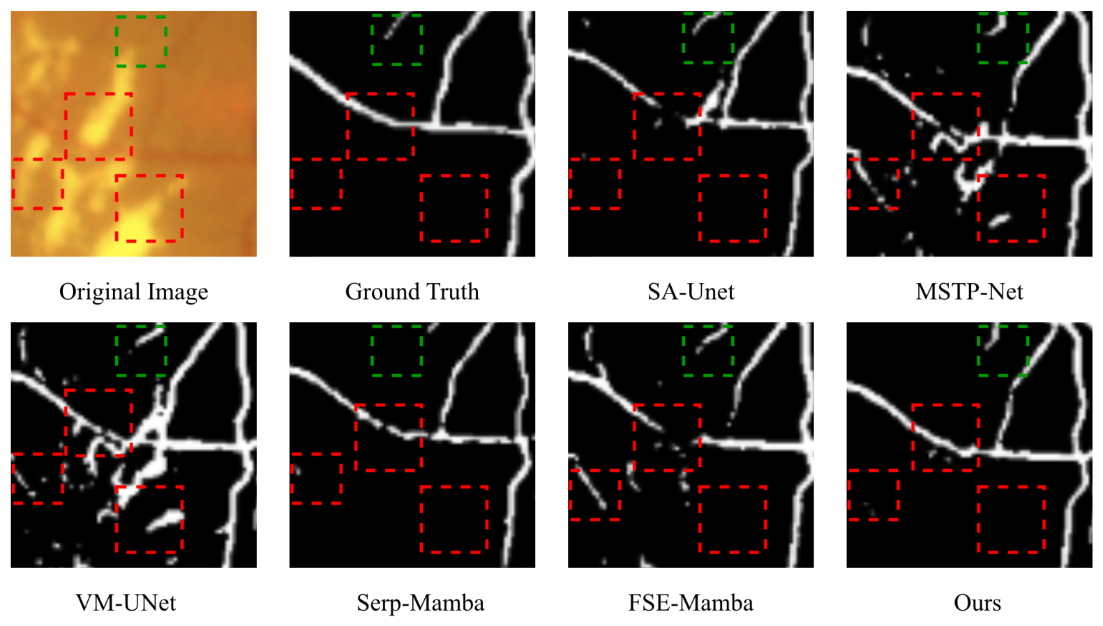
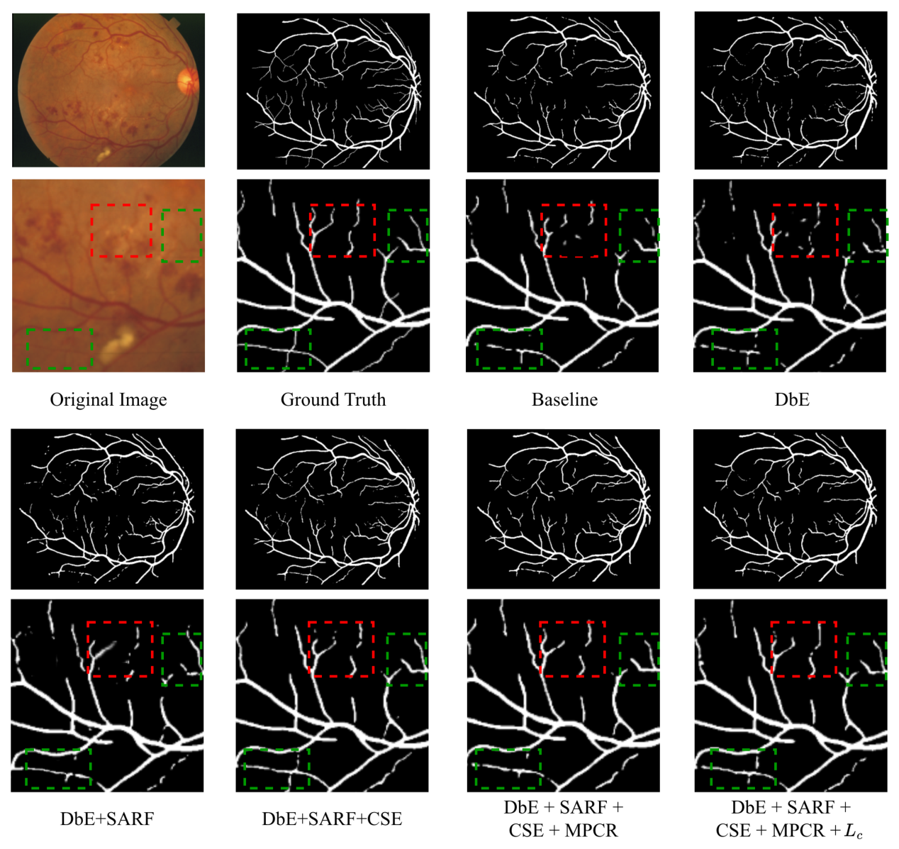
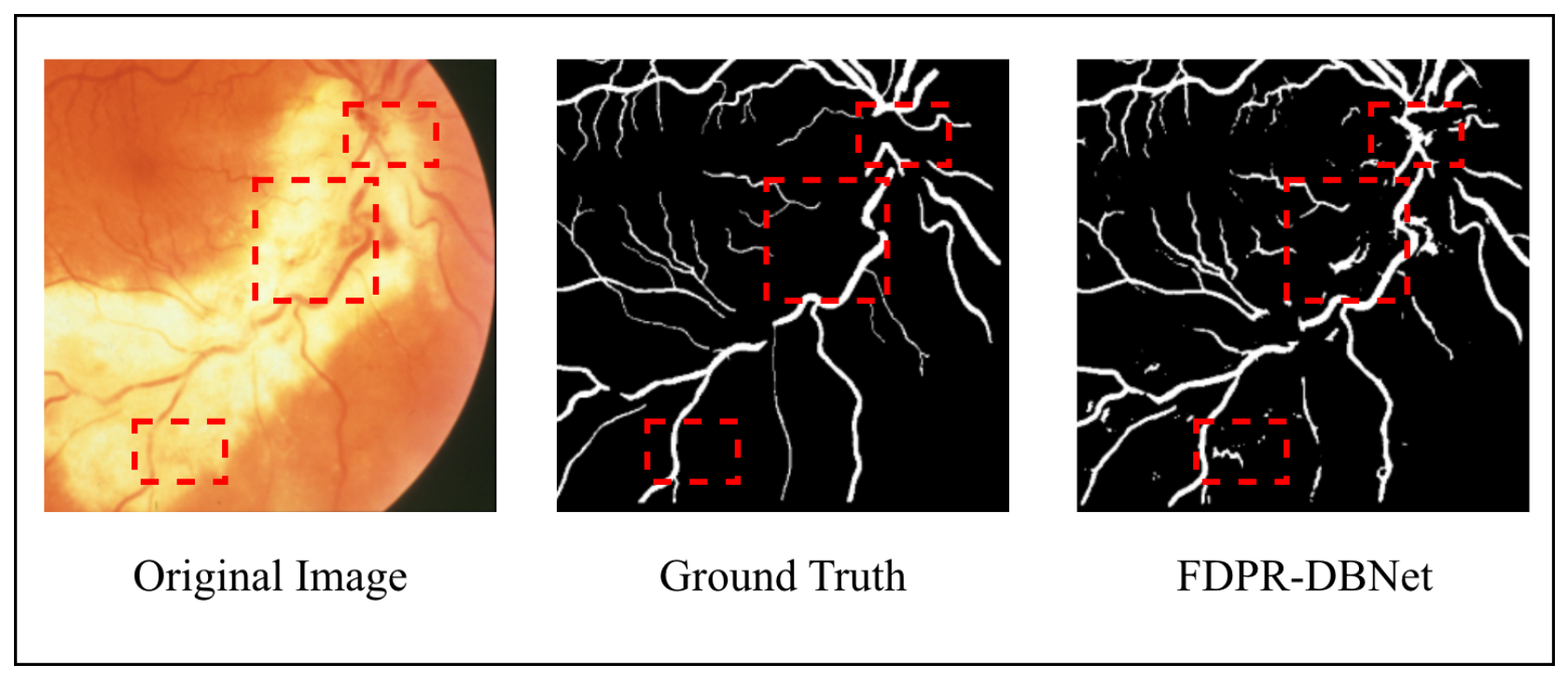
In the challenging regions containing fine capillaries (indicated by the red and green dashed boxes in Figure 19), our network faithfully reconstructed the intricate structures, whereas SA-UNet and Serp-Mamba suffered from severe discontinuities or missed vessels. Furthermore, the regions outlined in red represent areas heavily obscured by diabetic retinopathy (DR) lesions. These pathological interferences typically induced high false-positive rates; as a result, competing models such as VM-UNet and FSE-Mamba exhibited large-scale missegmentations. In contrast, our model could suppress these pathological interferences and delineate comparatively accurate vascular boundaries. In general, our model could preserve the topological integrity of thin vessels and minimize the adverse effects of fundus lesions in retinal images.

4.7. Cross-Dataset Generalization Evaluations

To assess the generalizability of FDPR-DBNet, we conducted cross-dataset vessel segmentation experiments on the DRIVE, CHASE_DB1, and STARE datasets and compared our model with current state-of-the-art methods. We trained each model on one dataset and tested it on the other two, alternating the training dataset. Table 8, Table 9 and Table 10 list the generalization comparison results of different methods across these three datasets. Herein, we define experimental scheme 1 as training on the STARE dataset and testing on the DRIVE and CHASE_DB1 datasets. Experimental scheme 2 is defined as training on the CHASE_DB1 dataset and testing on the DRIVE and STARE datasets. The remaining configuration, which involves training on the DRIVE dataset and testing on the STARE and CHASE_DB1 datasets, is termed experimental scheme 3. It was obvious from these tables that the proposed model consistently delivered overall optimal performance across most evaluation metrics in all experimental scenarios, validating its powerful generalizability and robustness. Among them, Serp-Mamba integrated a serpentine interwoven adaptive scan mechanism into Mamba networks to capture long-range dependency correlations in vessels. Nevertheless, it showed weaker generalization capabilities compared with our designed FDPR-DBNet. In Experimental Scheme 1, the ACC of Serp-Mamba exhibited a negligible improvement (0.03%) compared to ours on the DRIVE dataset, while its SP value rose by roughly 1.24% on the CHASE_DB1 dataset. However, our model achieved substantial improvements of 5.15%, 4.17%, 3.21%, and 0.11% in SE, Dice, PR, and AUC, respectively, on the DRIVE dataset, as well as increases of 1.54%, 2.15%, 2.72%, and 0.25% on the CHASE_DB1 benchmark. In Experimental Scheme 2, a similar trend could also be observed between our model and Serp-Mamba. Recently, FSE-Mamba introduced multi-scale axial attention and frequency-domain guided attention into the Mamba network to strengthen the global perception of vascular features and model inter-frequency relationships. However, it still showed limited cross-dataset generalization capability relative to our model.
For example, in experimental scheme 3, although FSE-Mamba obtained a higher overall ACC (97.93% vs. 96.32% for the STARE dataset, and 97.81% vs. 96.48% for the CHASE_DB1 dataset), our model maintained a notable gain in other critical segmentation indicators. The SE, Dice, and AUC of our model outweighed those of the baselines by 3.97%, 2.06%, and 1.21%, as well as 1.66%, 2.32%, and 0.54%, on these two datasets, respectively.These results showed that our model still retained high performance even under domain shifts, successfully suppressing noise while maintaining fine vessel skeleton structures on different external datasets. Upon further analysis of these tables, it could be seen that when testing on the STARE dataset after training on the DRIVE dataset, nearly all models brought a performance boost in terms of the SE indicator compared to their reverse scenario. This phenomenon could primarily be attributed to two factors: on the one hand, there existed inherent visual differences between these two datasets. The images from the DRIVE dataset were characterized by darker tones and lower contrast, whereas those from the STARE dataset were noticeably brighter with higher contrast. This clear visual property of fundus images from the STARE dataset contributed to vessel recognition. On the other hand, relatively few thin vessels were annotated in the STARE benchmark, and when the models trained on this dataset were transferred to the DRIVE dataset for testing, they could not accurately segment thin vessels.


4.8. Ablation Experiments

4.8.1. Ablation Study on Modules

To investigate the effect of each core component of FDPR-DBNet on segmentation performance, we conducted ablation experiments on the DRIVE dataset. A baseline was first constructed, after which the other components were sequentially integrated and tested. The baseline followed a U-shaped architecture with a three-stage dual-branch encoder, with each stage comprising standard 3 × 3 convolution blocks. The experimental results are presented in Table 11 and Figure 20, respectively. It was apparent that each designed component raised network performance, culminating in our proposed model that exceeded all other variants. The efficacy of each module was discussed as follows:
Effectiveness of Dual-branch encoder: We isolated the low-frequency (LF) from high-frequency (HF) sub-bands using wavelet decomposition and separately provided them to the encoder of the baseline to assess their individual influence. As summarized in Table 11, using only the HF sub-band along with the PACA module led to a decline in performance compared to the baseline, with SE and Dice dropping from 74.32% to 74.24% and from 76.51% to 76.06%, respectively. While the HF component was sensitive to fine-grained details, it struggled to maintain the topological connectivity of thick vessels due to its susceptibility to background noise. In contrast, the LF sub-band accompanied by SFCA yielded superior structural integrity, representing an SE improvement of 1.90% and a Dice gain of 0.83%. The LF information preserved the overall vessel structures, yet it often failed to capture delicate capillaries. Notably, by synergistically integrating the LF and HF sub-bands (denoted as DbE) through a CFF block, the performance significantly rose, reaching 80.51% (SE) and 81.15% (Dice), representing an amelioration of 6.19% and 4.64% over the baseline. Simultaneously, consistent enhancements were observed across other key metrics, with ACC, PR, and AUC increasing by 0.79%, 2.96%, and 0.66%, respectively.
From a qualitative perspective (as illustrated in Figure 20), it could also be observed that the high-frequency branch alone (Figure 20d) exhibited limitations in maintaining the topological continuity of the blood vessels. Conversely, utilizing only low-frequency information (Figure 20e) lacked attention to microvessels. By comparison, the dual-branch encoder (Figure 20f) struck an optimal balance between maintaining structural continuity and preserving fine details. These results reiterated that the low-frequency branch ensured the structural continuity of thick vessels, whereas the high-frequency branch captured fine-grained details essential for boundary localization and capillary detection. Our dual-branch encoder provided complementary feature representations on the intricate retinal vascular network.
Effectiveness of SARF component: In the following, we inserted the SARF module between the dual-branch encoder to enable the interaction between high- and low-frequency features. As shown in row five of Table 11, the inclusion of the SARF module further bolstered the model’s overall performance, with SE, SP, Dice and ACC increasing by 1.62%, 0.75%, 0.53% and 0.73%, respectively. On top of the visualization results from Figure 20f,g, the addition of the SARF block effectively improved the integrity and continuity of major vessel structure alongside edge sharpness, while suppressing non-vessel noise. These confirmed the effectiveness of utilizing the SARF component to strengthen complementary feature exchange between the dual-branch encoder.
Effectiveness of CSE unit combining GSE with LDE: After incorporating GSE and LDE step by step, we verified their effects on the model’s performance individually. As indicated in rows six and seven of Table 11, introducing the LDE module resulted in 0.24%, 1.68%, 1.87%, and 1.78% increments in ACC, SE, PR, and Dice compared to Baseline+DbE+SARF. When the GSE block was further applied as a bottleneck layer (defined as DbE + SARF + CSE), the Dice increased by 1.55%, and all other evaluation metrics also showed corresponding improvements. The visual segmentation effects, as shown in Figure 20h,i, reflected that the segmentation of the vessel backbone structure was more complete, while the low-contrast thin vessels and boundary details were also clearly outlined after integrating LDE and GSE. These results substantiated that placing a CSE unit had a positive influence on segmentation performance, and its absence limited comprehensive pattern expression pertinent to retinal blood vessels.
Effectiveness of MPCR component: Row 8 of Table 11 presented the outcomes after appending the MPCR block. Compared to DbE + SARF + CSE, the removal of the MPCR component brought an obvious deterioration across nearly all indicators, reducing scores of ACC, SE, SP, PR, and Dice by 0.30%, 1.84%, 0.67%, 0.99%, and 1.46%, respectively. The visual segmentation effects, as displayed in Figure 20j, indicated further enhancements in the clarity of thin blood vessel boundaries compared to those without the MPCR module. These findings demonstrated that the MPCR component effectively facilitated cross-scale semantic correction and alignment in the decoder via a dynamic feature calibration mechanism, thereby retaining and enhancing vessel boundary integrity within characteristic representations.
As evidenced by the ablation study results in Table 11, the DbE (CFF) module provided the most significant performance gain, bringing improvements of 4.64% and 7.34% in Dice and clDice, respectively, when compared to the Baseline. It introduced a minor parameter increment of 0.58 M and a FLOP increase of 0.91 G, while obtaining a high inference speed of 87.45 FPS. Building upon this, the integration of the SARF block raised the clDice score from 74.68% to 76.50% with a minimal increase in computational overhead ( Δ Params = 0.25 M and Δ FLOPs = 0.53 G ). Incorporating the LDE module into the “+DbE + SARF” baseline introduced a minor parameter increment of 0.37 M (from 2.68 M to 3.05 M) and a computational expansion of 0.77 GFLOPs (from 3.58 G to 4.35 G). Furthermore, adding the GSE module brought a similarly well-controlled computational overhead ( Δ Params = 0.43 M and Δ FLOPs = 0.77 G ). Collectively, the LDE and GSE components yielded a total increase of 0.8 M parameters and 1.54 GFLOPs while sacrificing only 6.06 FPS (from 85.10 FPS down to 79.04 FPS) of inference speed. However, this brought substantial segmentation performance improvements, with Dice rising from 81.68% to 85.01% (+3.33%) and clDice elevating from 76.50% to 79.68% (+3.18%). In contrast, when introducing the MPCR block, the model’s performance reached its optimum while still maintaining a high inference speed of 78.18 FPS, wherein the Dice score increased by 1.46% at the cost of a parameter growth of 0.25 M and 0.55 G in FLOPs.
Effect of weight factor λ in loss function: Since the proposed connectivity loss L C was normalized by the total number of pixels, its numerical scale inherently correlated with the image resolution, and the substantial resolution discrepancies across different datasets indeed posed a theoretical challenge to the generalization stability of the balancing coefficient λ . Nevertheless, it was adopted based on two paramount mathematical considerations: (1) Normalizing by target vessel pixels yielded a highly volatile denominator, particularly in images where the target vessel was extremely scarce. Total pixel normalization avoided this mathematical singularity and stabilized backpropagation. (2) Structural connectivity optimization required a global frame of reference. Normalizing by the total number of pixels within the image scaled the loss proportional to the total background distribution, encouraging the model to maintain topological continuity globally. In addition, in our model, re-tuning of λ across datasets could also be mitigated by our standardized resolution preprocessing pipeline. To rigorously evaluate the generalization stability of λ under varying resolutions, we conducted a hyperparameter sensitivity analysis across different datasets with diverse resolutions (including DRIVE at 584 × 565, STARE at 700 × 605, CHASE_DBl at 999 × 960, and IOSTAR at 1024 × 1024). As illustrated in Figure 21, the optimal performance metrics were attained when λ = 1 on the low-resolution DRIVE and STARE datasets, whereas they were attained at λ = 1.2 on the high-resolution CHASE_DBl and IOSTAR datasets. When λ varied from 1 to 1.2, only slight variations between 85.55% and 85.67% on CHASE_DB1 and between 85.43% and 85.51% on IOSTAR in terms of Dice were observed. This indicated that the model maintained robust performance boundaries under a steady range of λ , validating the practical scalability of connectivity loss L C . Considering accurate segmentation and topology preservation, we set λ = 1 as a trade-off.

4.8.2. Comparison with Various Fusion Mechanisms

To emphasize the benefits of the key components in the proposed FDPR-DBNet, we developed four variants by sequentially replacing SARF with three popular fusion methods: addition, CBAM, and Residual Fusion on the DRIVE dataset. The quantitative results and qualitative visualizations were presented in Table 12 and Figure 22, respectively. The baseline model, DbE, achieved an ACC of 96.38% and an AUC of 98.23%.
When introducing a simple element-wise addition (+Add), we observed marginal changes across most metrics, indicating that naive linear fusion is insufficient to fully capture the complex, non-linear correlations between high-frequency fine details and low-frequency global contexts. Incorporating the standard convolutional block attention module (+CBAM) improved the ACC to 96.75% and SE to 81.18%, demonstrating the benefit of utilizing channel and spatial attention to recalibrate frequency features. Furthermore, the residual fusion mechanism (+Residual Fusion) yielded a noticeable boost in SP to 98.46% and SE to 81.98%, confirming that preserving multi-scale residual paths helped mitigate the loss of subtle high-frequency edge information during deep feature transmission.
Ultimately, our proposed method (+SARF) outperformed all other configurations, achieving the highest performance across almost all key metrics, including an ACC of 97.11%, SE of 82.13%, SP of 98.82%, and Dice of 81.68%. These substantial improvements strongly demonstrated that the SARF can dynamically align and adaptively fuse cross-frequency representations. By effectively highlighting critical high-frequency textures while preserving stable low-frequency structures, the proposed SARF successfully maximized the synergy between different frequency streams, leading to superior segmentation robustness. As illustrated by the Grad-CAM visualizations in Figure 22, the proposed model precisely localized critical regions of the retinal vasculature, yielding highly interpretable saliency heatmaps. Notably, these visual results further confirmed that our method exhibited superior efficacy in capturing fine microvascular structures compared to alternative approaches.

4.8.3. Comparison with Other Loss Functions

Aiming to validate the rationality of our proposed connectivity loss, we compared it against other topology-preserving losses, including clDice loss [51], BettiLoss [52], and TopoLoss [53]. We selected the designed model framework as the backbone, and all configurations utilized the same backbone with the exception of the loss function to ensure fairness. As summarized in Table 13 and Figure 23, the model utilizing the designed connectivity loss outperformed these specialized loss-driven baselines across nearly all primary segmentation and topological metrics. For instance, it achieved the top score of 80.19% in the clDice metric, outperforming those based on clDice loss (79.87%), BettiLoss (77.63%), and TopoLoss (76.76%). This demonstrated that our connectivity loss strategy was more effective at maintaining vascular continuity than alternative topology preservation approaches.

4.8.4. Qualitative Evaluation of Progressive Module Contributions

To further investigate the intuitive impact of each proposed component, we provided a qualitative visualization demonstrating the progressive segmentation enhancements in Figure 24. Several challenging regions of interest (ROIs) encompassing microvascular networks outlined in green dashed boxes and lesion-prone areas highlighted in red dashed boxes were magnified for close inspection. As illustrated in Figure 1, the Baseline and DbE variants suffered from severe vessel fragmentation and missed thin capillaries due to low local contrast and pathological artifacts. Upon incorporating the SARF module, the contrast of tiny peripheral vessels was distinctly reinforced, allowing the model to recover vascular fragments that were previously drowned out by the background and pathological artifacts. Furthermore, the inclusion of the CSE module successfully bridged major structural gaps in the intermediate vascular tree by aggregating multi-scale local details and long-range global contexts, improving vascular morphology continuity. When the MPCR module was activated, well-demarcated thin-vessel boundary delineations were observed through prototype-guided feature correction and alignment, especially in regions clustered with confounding pathological artifacts. Finally, the introduction of the proposed connectivity loss served as a vital topological constraint that explicitly penalized structural disconnections. It bridged the remaining gaps in the fine capillaries, successfully restoring the capillary endpoints and ensuring structural continuity that matched the ground truth. This progressive visual evolution underscored that each component played a complementary and indispensable role in solving the intrinsic challenges of retinal vessel segmentation.
Finally, we show the intermediate feature maps for each stage in Figure 25. By comparing the corresponding high- and low-frequency feature maps across stages 1–3 in Figure 25a,b, it can be observed that under the interactive guidance of the spatial attention residual fusion (SARF) module, the model extracts critical boundary features of blood vessels at different scales from the high-frequency branch and effectively suppresses non-vascular noise, while strengthening vascular regional context learning and optimizing low-frequency region feature representations by propagating these refined edge cues into the low-frequency region branch. Furthermore, we can also observe that the cross-frequency fusion (CFF) module allows the model to learn more comprehensive feature expressions, forming a powerful encoding representation. Concurrently, the feature maps from the local detail enhancement (LDE) units at different stages exhibited a highly concentrated, sharp response along the delicate peripheral capillaries and vessel boundaries. After the CFF module, the Transformer-driven global semantic enhancement (GSE) block produced an attention map that seamlessly outlined the long-range topology of the entire vascular tree. This demonstrated that the GSE block successfully captured long-distance feature dependencies, preventing premature vessel fragmentation. The feature maps of the multi-wise prototype characteristic refinement (MPCR) module displayed a remarkably clean, high-contrast vascular skeleton. Background tissue textures, optic discs, and potential pathological lesions were entirely suppressed, leaving only pure semantic vascular paths. This verified that the prototype refinement process effectively served as a clean semantic filter through a dynamic feature calibration mechanism. At last, the progression through DConv Block 1, DConv Block 2, and DConv Block 3 reflected the decoder’s exceptional ability to adaptively fit the highly curved and tortuous geometric morphology of retinal blood vessels.

4.9. Statistical Significance Testing

In order to investigate the statistical reliability of the observed performance improvements between our proposed model and other methods, we conducted paired t-tests across eight evaluation indicators on four publicly available datasets: DRIVE, CHASE_DB1, STARE, and IOSTAR. The statistical p-values were presented in Table 14 and Table 15 on these four retinal datasets. The results indicated that our model exhibited widespread statistically significant improvements over almost all established baseline methods across most evaluation metrics (p < 0.05), with a substantial number reaching high statistical significance (p < 0.01). It kept a highly competitive and statistically superior advantage over contemporary advanced Transformer- and Mamba-based methods in critical segmentation indicators like Dice and SE. These findings indicated that the observed performance benefits of our model were statistically robust and not the result of random variation.

4.10. Model Complexity Analysis

Finally, we evaluated the computational overhead and segmentation efficacy of FDPR-DBNet against state-of-the-art methods on the DRIVE dataset. The quantitative results and visual trade-offs are presented in Table 16 and Figure 26, respectively. As displayed in Table 16 and Figure 26, our model delivered a high inference speed of 78.18 FPS and a low inference latency per case of 12.79 ms only requiring 15.44 MB of GPU peak memory during inference, which was approximately 2.3× faster than VM-UNet (33.23 FPS and 30.09 ms), and 1.7× faster than TransUNet (45.47 FPS and 21.99 ms). It brought an obvious reduction in inference time per case, being 17.30 ms and 9.20 ms shorter than VM-UNet and TransUNet, respectively. When compared with the comparatively lightweight model SA-UNet, our model showed a slight decline in inference performance, including inference speed dropping from 88.64 FPS to 78.18 FPS, inference time per case rising from 11.28 ms to 12.79 ms, and inference memory footprint increasing from 6.42 MB to 15.44 MB. However, these costs were justified by a significant Dice score enhancement from 79.73% to 86.47%. When compared with FSE-Mamba, our model occupied less peak memory during training (4.89 GB vs. 6.11 GB) and inference (15.44 MB vs. 97.28 MB) and required shorter training time per epoch (8.01 s vs. 10.42 s) and inference time per case (12.79 ms vs. 15.97 ms), whilst achieving the best segmentation performance (Dice: 86.47% vs. 81.18%). Our model also maintained an efficient computational footprint of 3.73 M params and 5.67 GFLOPs, outperforming FSE-Mamba (25.50 M Params/6.32 GFLOPs) operating within a frequency-domain framework. While models like FreqUNet (0.26M Params and 1.40G FLOPs) and LadderNet (2.88 M Params and 2.19 G FLOPs) were lighter than our model, these overheads were justified by a substantial Dice score improvement from 75.82% to 86.47% and from 77.75% to 86.47%, respectively. These results indicated that our model was better suited for retinal vessel segmentation as a result of its superior computational efficiency and segmentation accuracy.
While our model has so far been validated on a high-performance workstation equipped with an NVIDIA GeForce RTX 4070 Ti GPU, adopting parallel edge computing or embedded platforms represents a more suitable and promising direction for practical clinical deployment. As highlighted by recent research on embedded parallel architectures for ocular disease screening [54], leveraging deep learning models on resource-constrained embedded devices could substantially improve diagnostic efficiency and scalability. In future work, we plan to further optimize and compress our model to facilitate its deployment on such embedded edge devices.

5. Conclusions and Future Work

In this paper, we developed FDPR-DBNet, a novel dual-branch network with frequency-aware decomposition and prototype refinement tailored for cross-frequency adaptive feature interaction and multi-scale feature perception and calibration, thereby improving retinal vessel segmentation accuracy. Within the dual-branch encoder, we introduced SFCA and PACA modules to adaptively capture refined local high-frequency boundary details and informative global low-frequency regional characteristics, respectively. Concurrently, both SARF and CFF components were constructed within the dual-branch encoder to promote mutual guidance and adaptive fusion of frequency-aware region and boundary characteristics, enabling the model to learn comprehensive feature representations of blood vessels. Furthermore, the CSE unit, composed of GSE and LDE components, was incorporated into the skip connections to progressively couple multi-scale features across adjacent encoding levels, reducing semantic bias across multiple scales and amplifying target response signals in deep features, thereby enhancing the model’s sensitivity and accuracy when identifying fine vessels. In addition, we created an MPCR module based on a dynamic feature calibration strategy in the decoder to facilitate the correction and alignment of cross-scale semantic information, ensuring vascular boundary integrity and salience. Furthermore, we applied a connectivity loss function to maintain vessel continuity and topology by penalizing fragmented segments. Both quantitative and qualitative comparisons with state-of-the-art methods on four benchmark retinal fundus image datasets indicated that FDPR-DBNet achieved state-of-the-art segmentation performance without sacrificing computational efficiency and demonstrated strong cross-dataset generalizability. Even in the presence of complex ocular pathologies, our model demonstrated excellent segmentation performance. Moreover, comprehensive ablation studies confirmed the contribution of each key component.
Retinal vascular morphology contains pivotal diagnostic biomarkers for systemic and ocular diseases (such as diabetic retinopathy, hypertension, and atherosclerosis). The highly accurate and complete preservation of vascular topology achieved by FDPR-DBNet when delineating both major vessel backbones and delicate peripheral capillaries facilitated the automated, objective extraction of clinical parameters such as the arteriole-to-venule ratio (AVR), vessel tortuosity indices, and fractal dimensions. In real-world clinical deployment, processing speed and hardware footprint are crucial benchmarks. Running on standard clinical workstations without requiring high-end computing systems, FDPR-DBNet sustained an inference speed of over 78 FPS, requiring 15.44 MB of GPU memory during inference while maintaining a low computational cost (3.73 M Params and 5.67 G FLOPs), significantly exceeding the standard real-time requirement for clinical applications (30 FPS). This high efficiency allowed it to serve as a fast, non-invasive screening tool embedded in fundus camera software, aiding clinicians by automatically highlighting subtle microvascular alterations or proliferative changes before manual visual inspection.
Although FDPR-DBNet demonstrated remarkable segmentation performance, several important limitations warrant consideration and point to potential directions for future research. First, our model was restricted to DWT-based frequency decomposition. In future work, alternative transform techniques, such as contourlet, shearlet, or Gabor transforms, may warrant in-depth exploration to capture more directional and curvilinear vascular patterns. Second, despite the rigorous evaluation using diseased retinal images, the limited diversity of the test data may not fully reflect our model’s segmentation performance across a wider range of pathologies. Future work could address this limitation by enriching the data repository with more diverse pathologies and imaging conditions. Finally, our model still exhibited some difficulty distinguishing subtle vessels from the background when faced with noisy or cluttered images. Future work will focus on developing more effective multi-scale feature extraction and data augmentation techniques to improve segmentation performance in such complex scenarios.

6. Discussion

Although Mamba-based segmentation methods exhibited superior ability to capture the global spatial context of vessels, their effectiveness was severely constrained by background noise, pathological interference, and artifacts in low-contrast retinal images, thereby impairing the localization of small-vessel regions. Compared with the global spatial features extracted by Mamba-based segmentation approaches, frequency-aware segmentation methods were more sensitive to noise patterns and boundaries, enabling frequency-aware features to effectively handle vessel edges and image noise. Yet, they primarily suffered from a lack of effective cross-frequency interaction between boundary and regional features across different scales, inevitably causing vascular structure fragmentation and disconnection. In contrast, our model addressed these shortcomings through several core innovations. First, frequency-domain feature decomposition mapped high-frequency features to spatial edges and low-frequency features to spatial areas, which helped the model retain critical high-frequency boundary components while enhancing regional feature representation through the hierarchical spatial-frequency characteristic activation (SFCA) and parallel atrous convolution activation (PACA) modules. Second, adaptive cross-frequency fusion and mutual guidance between complementary boundary and regional features at multiple scales were achieved by combining a spatial attention residual fusion (SARF) unit with a cross-frequency fusion (CFF) block, thereby propagating refined boundary cues to optimize regional context learning and minimize noise interference. This dual-branch architecture guided the model to capture more universal retinal vessel features by combining the advantages of frequency-domain processing for boundary and region perception. Finally, the multi-wise prototype characteristic refinement (MPCR) module was introduced into the decoder to align cross-scale semantic information via a dynamic feature calibration mechanism, thereby preserving structural integrity in feature representations. In conjunction with this, a new connectivity loss function was developed to penalize fragmentation in the vascular network and maintain the topological continuity of vascular structures.
In vascular segmentation tasks, the target vessel pixels typically occupied a tiny fraction (often <10%) of the entire retinal image. Under such extreme class imbalance, evaluating models solely based on ACC could be highly misleading. A naive model could also achieve a deceptively high ACC by simply favoring background predictions and over-suppressing thin and complex vessel boundaries. Conversely, the Dice coefficient, which was mathematically equivalent to the F1-score in binary classification tasks, directly measured the overlap between the predicted and ground-truth vessel pixels without being dominated by the vast background regions. Meanwhile, the AUC gauged the model’s overall discrimination capability across various decision thresholds, making it more robust to class distribution shifts. Clinically, Dice and AUC served as more informative and reliable indicators of segmentation quality. While certain previous methods, such as Serp-Mamba, exhibited competitive ACC values by tending toward background predictions, our model significantly outperformed them by 2.64% and 0.11% in Dice and AUC, respectively. This demonstrated our model’s superior capability to capture continuous topological structures and fine boundary cues, which were of greater significance for clinical diagnosis.
In real-world clinical scenarios where images frequently suffer from severe degradation or complex pathologies, our model still carries the risk that noise from the high-frequency branch may contaminate the low-frequency main branch through cross-branch interaction, thereby disrupting the structural topology and inducing spurious microvessel segments. As observed in Table 11, when used independently, the high-frequency branch exhibited a performance drop (the Dice score decreased from 76.51% to 76.06%) compared with the baseline. However, the designed spatial attention residual fusion (SARF) component enabled adaptive, selective fusion and mutual guidance between high-frequency boundary and low-frequency region features at different scales in the encoder by introducing a residual spatial attention mechanism. This mechanism helped mitigate the contamination of low-frequency regional features by noisy signals captured by the high-frequency branch. As shown in Table 11, integrating the two branches by combining the SARF and CFF modules resulted in a substantial performance improvement, with the Dice score increasing to 81.15%. In real-world clinical scenarios where images frequently suffer from severe degradation or complex pathologies, our model still faces the risk that noise from the high-frequency branch may contaminate the low-frequency main branch through cross-branch interaction, thereby disrupting the structural topology and inducing spurious microvessel segments. Figure 27 illustrates a representative segmentation failure by our model caused by interference from severe retinal pathology, characterized by extensive, high-contrast bright lesions such as dense exudates or chorioretinal scarring. The model misidentified pathological retinal regions as microvessels, resulting in false-positive predictions. In future work, we plan to introduce a lesion-aware gating mechanism into the dual-branch network to mitigate the risk of high-frequency noise contamination under severe pathological conditions and improve the model’s robustness.

Author Contributions

Conceptualization, F.L.; methodology, F.L. and Y.F.; software, Y.F.; validation, Y.F.; investigation, Y.F.; writing—original draft preparation, Y.F.; writing—review and editing, F.L.; visualization, Y.F.; supervision, F.L.; funding acquisition, F.L. All authors have read and agreed to the published version of the manuscript.

Funding

This work was supported by the National Key Research and Development Program of China (Grant No. 2021YFB2802303), the National Natural Science Foundation of China (Grant No. 51675321).

Data Availability Statement

The original contributions presented in this study are included in the article. Further inquiries can be directed to the corresponding author.

Conflicts of Interest

The authors declare no conflicts of interest.

References

  1. Miri, M.; Amini, Z.; Rabbani, H.; Kafieh, R. A Comprehensive Study of Retinal Vessel Classification Methods in Fundus Images. J. Med. Signals Sens. 2017, 7, 59–70. [Google Scholar] [CrossRef] [Scilit] [PubMed]
  2. Seo, H.; Park, S.J.; Song, M. Diabetic Retinopathy (DR): Mechanisms, Current Therapies, and Emerging Strategies. Cells 2025, 14, 376. [Google Scholar] [CrossRef] [Scilit] [PubMed]
  3. Cervantes, J.; Cervantes, J.; García-Lamont, F.; Yee-Rendon, A.; Cabrera, J.E.; Jalili, L.D. A comprehensive survey on segmentation techniques for retinal vessel segmentation. Neurocomputing 2023, 556, 126626. [Google Scholar] [CrossRef] [Scilit]
  4. Li, X.; Lu, S.; Liu, J.; Zhu, P.; Zhang, H. Signal Image Processing Based on Matched Filtering. In 2025 International Conference on Computational Intelligence and Robotics (CIR); IEEE: Piscataway, NJ, USA, 2025; pp. 159–166. [Google Scholar] [CrossRef] [Scilit]
  5. Kimori, Y. Morphological image processing for quantitative shape analysis of biomedical structures: Effective contrast enhancement. J. Synchrotron Radiat. 2013, 20, 848–853. [Google Scholar] [CrossRef] [Scilit] [PubMed]
  6. Jia, D.; Zhuang, X. Learning-based algorithms for vessel tracking: A review. Comput. Med. Imaging Graph. 2021, 89, 101840. [Google Scholar] [CrossRef] [Scilit] [PubMed]
  7. Sarker, I.H. Machine Learning: Algorithms, Real-World Applications and Research Directions. SN Comput. Sci. 2021, 2, 160. [Google Scholar] [CrossRef] [Scilit] [PubMed]
  8. Ronneberger, O.; Fischer, P.; Brox, T. U-Net: Convolutional Networks for Biomedical Image Segmentation. In Medical Image Computing and Computer-Assisted Intervention—MICCAI 2015; Springer: Cham, Switzerland, 2015; pp. 234–241. [Google Scholar] [CrossRef] [Scilit]
  9. Zhang, Y.; Li, Z.; Nan, N.; Wang, X. TranSegNet: Hybrid CNN-Vision Transformers Encoder for Retina Segmentation of Optical Coherence Tomography. Life 2023, 13, 976. [Google Scholar] [CrossRef] [Scilit] [PubMed]
  10. Tragakis, A.; Liu, Q.; Kaul, C.; Roy, S.K.; Dai, H.; Deligianni, F.; Murray-Smith, R.; Faccio, D. GLFNet: Global-Local (frequency) Filter Networks for efficient medical image segmentation. In 2024 IEEE International Symposium on Biomedical Imaging (ISBI); IEEE: Piscataway, NJ, USA, 2024; pp. 1–5. [Google Scholar] [CrossRef] [Scilit]
  11. Li, P.; Zhou, R.; He, J.; Zhao, S.; Tian, Y. A global-frequency-domain network for medical image segmentation. Comput. Biol. Med. 2023, 164, 107290. [Google Scholar] [CrossRef] [Scilit] [PubMed]
  12. Zou, Z.; Yu, H.; Zhao, F. FreqMamba: Viewing Mamba from a Frequency Perspective for Image Deraining. arXiv 2024, arXiv:2404.09476. [Google Scholar] [CrossRef] [Scilit]
  13. Qin, Q.; Chen, Y. A review of retinal vessel segmentation for fundus image analysis. Eng. Appl. Artif. Intell. 2024, 128, 107454. [Google Scholar] [CrossRef] [Scilit]
  14. Zhuang, J. LadderNet: Multi-path networks based on U-Net for medical image segmentation. arXiv 2018, arXiv:1810.07810. [Google Scholar]
  15. Gu, Z.; Cheng, J.; Fu, H.; Zhou, K.; Hao, H.; Zhao, Y.; Zhang, T.; Gao, S.; Liu, J. CE-Net: Context Encoder Network for 2D Medical Image Segmentation. IEEE Trans. Med. Imaging 2019, 38, 2281–2292. [Google Scholar] [CrossRef] [Scilit] [PubMed]
  16. Huang, H.; Lin, L.; Tong, R.; Hu, H.; Zhang, Q.; Iwamoto, Y.; Han, X.; Chen, Y.W.; Wu, J. UNet 3+: A Full-Scale Connected UNet for Medical Image Segmentation. In 2020 IEEE International Conference on Acoustics, Speech and Signal Processing (ICASSP); IEEE: Piscataway, NJ, USA, 2020; pp. 1055–1059. [Google Scholar] [CrossRef] [Scilit]
  17. Guo, C.; Szemenyei, M.; Yi, Y.; Wang, W.; Chen, B.; Fan, C. SA-UNet: Spatial Attention U-Net for Retinal Vessel Segmentation. In 2020 25th International Conference on Pattern Recognition (ICPR); IEEE: Piscataway, NJ, USA, 2021; pp. 1236–1242. [Google Scholar] [CrossRef] [Scilit]
  18. Ding, W.; Sun, Y.; Huang, J.; Ju, H.; Zhang, C.; Yang, G.; Lin, C.T. RCAR-UNet: Retinal vessel segmentation network algorithm via novel rough attention mechanism. Inf. Sci. 2024, 657, 120007. [Google Scholar] [CrossRef] [Scilit]
  19. Wang, J.; Li, X.; Ma, Z. Multi-Scale Three-Path Network (MSTP-Net): A new architecture for retinal vessel segmentation. Measurement 2025, 250, 117100. [Google Scholar] [CrossRef] [Scilit]
  20. Yang, Y.; Sun, L.; Tang, Z.; Liu, G.; Zhou, G.; Li, L.; Cai, W.; Li, L.; Chen, L.; Hu, L. A precise image-based retinal blood vessel segmentation method using TAOD-CFNet. Biomed. Signal Process. Control 2025, 107, 107815. [Google Scholar] [CrossRef] [Scilit]
  21. Chen, J.; Lu, Y.; Yu, Q.; Luo, X.; Adeli, E.; Wang, Y.; Lu, L.; Yuille, A.L.; Zhou, Y. TransUNet: Transformers Make Strong Encoders for Medical Image Segmentation. arXiv 2021, arXiv:2102.04306. [Google Scholar] [CrossRef] [Scilit]
  22. Zhang, H.; Ni, W.; Luo, Y.; Feng, Y.; Song, R.; Wang, X. TUnet-LBF: Retinal fundus image fine segmentation model based on transformer Unet network and LBF. Comput. Biol. Med. 2023, 159, 106937. [Google Scholar] [CrossRef] [Scilit] [PubMed]
  23. Lin, J.; Huang, X.; Zhou, H.; Wang, Y.; Zhang, Q. Stimulus-guided adaptive transformer network for retinal blood vessel segmentation in fundus images. Med. Image Anal. 2023, 89, 102929. [Google Scholar] [CrossRef] [Scilit] [PubMed]
  24. Luo, X.; Peng, L.; Ke, Z.; Lin, J.; Yu, Z. PA-Net: A hybrid architecture for retinal vessel segmentation. Pattern Recognit. 2025, 161, 111254. [Google Scholar] [CrossRef] [Scilit]
  25. Qiu, Y.; Zhang, H.; Song, C.; Zhao, X.; Li, H.; Wang, X. GKE-TUNet: Geometry–Knowledge Embedded TransUNet Model for Retinal Vessel Segmentation Considering Anatomical Topology. IEEE J. Biomed. Health Inform. 2024, 28, 6725–6737. [Google Scholar] [CrossRef] [Scilit] [PubMed]
  26. Liang, L.; Lu, B.; Wu, J.; Li, Y.; Sheng, X. SFIT-Net: Spatial Reconstruction Feature Interaction Transformer Retinal Vessel Segmentation Algorithm. Biomed. Signal Process. Control 2025, 106, 107688. [Google Scholar] [CrossRef] [Scilit]
  27. Gu, J.; Tian, F.; Oh, I.S. RAMIS: Increasing robustness and accuracy in medical image segmentation with hybrid CNN-transformer synergy. Neurocomputing 2025, 618, 129009. [Google Scholar] [CrossRef] [Scilit]
  28. Zhang, X.; Lv, W.R.; Lu, L.; Ye, Z.; Zhou, M.; Duan, J.; Su, Y.; Wang, S. SDHM2T: A scale direction heteroid micro to macro transition network for retinal vessel segmentation. Biomed. Signal Process. Control 2026, 113, 108881. [Google Scholar] [CrossRef] [Scilit]
  29. Ma, J.; Li, F.; Wang, B. U-Mamba: Enhancing Long-Range Dependency for Biomedical Image Segmentation. arXiv 2024, arXiv:2401.04722. [Google Scholar] [CrossRef] [Scilit]
  30. Liu, Y.; Tian, Y.; Zhao, Y.; Yu, H.; Xie, L.; Wang, Y.; Ye, Q.; Jiao, J.; Liu, Y. VMamba: Visual State Space Model. In Neural Information Processing Systems (NeurIPS); Curran Associates, Inc.: Red Hook, NY, USA, 2024. [Google Scholar]
  31. Ruan, J.; Li, J.; Xiang, S. VM-UNet: Vision Mamba UNet for Medical Image Segmentation. arXiv 2024, arXiv:2402.02491. [Google Scholar] [CrossRef] [Scilit]
  32. Zhang, M.; Yu, Y.; Gu, L.; Lin, T.; Tao, X. VM-UNet-V2: Rethinking Vision Mamba UNet for Medical Image Segmentation. arXiv 2024, arXiv:2403.09157. [Google Scholar] [CrossRef] [Scilit]
  33. Wang, H.; Chen, Y.; Chen, W.; Xu, H.; Zhao, H.; Sheng, B.; Fu, H.; Yang, G.; Zhu, L. Serp-Mamba: Advancing High-Resolution Retinal Vessel Segmentation with Selective State-Space Model. arXiv 2024, arXiv:2409.04356. [Google Scholar] [CrossRef] [Scilit]
  34. Liu, Y.; Xia, E.; Sun, C.; Zhou, Z. CRMA-UNet: CNN + ResMamba-based and attentional mechanisms for retinal vessel segmentation. Expert Syst. Appl. 2026, 297, 129286. [Google Scholar] [CrossRef] [Scilit]
  35. Xu, H.; Wu, Y. G2ViT: Graph Neural Network-Guided Vision Transformer Enhanced Network for retinal vessel and coronary angiograph segmentation. Neural Netw. 2024, 176, 106356. [Google Scholar] [CrossRef] [Scilit] [PubMed]
  36. Wang, H.; Kang, N.; Shi, Z.; Pan, X.; Lan, R.; Luo, X. Retinal vessel segmentation via bifurcation intensity driven and heterogeneous graph optimization. Knowl.-Based Syst. 2026, 336, 115345. [Google Scholar] [CrossRef] [Scilit]
  37. Qin, Z.; Zhang, P.; Wu, F.; Li, X. FcaNet: Frequency Channel Attention Networks. In 2021 IEEE/CVF International Conference on Computer Vision (ICCV); IEEE: Piscataway, NJ, USA, 2021; pp. 783–792. [Google Scholar] [CrossRef] [Scilit]
  38. Rao, Y.; Zhao, W.; Zhu, Z.; Lu, J.; Zhou, J. Global Filter Networks for Image Classification. In Advances in Neural Information Processing Systems (NeurIPS); Curran Associates, Inc.: Red Hook, NY, USA, 2021; Volume 34, pp. 980–993. [Google Scholar]
  39. Zhou, Y.; Huang, J.; Wang, C.; Song, L.; Yang, G. XNet: Wavelet-Based Low and High Frequency Fusion Networks for Fully- and Semi-Supervised Semantic Segmentation of Biomedical Images. In Proceedings of the IEEE/CVF International Conference on Computer Vision (ICCV); IEEE: Piscataway, NJ, USA, 2023; pp. 21085–21095. [Google Scholar] [CrossRef] [Scilit]
  40. Bo, Y.; Zhu, Y.; Li, L.; Zhang, H. FAMNet: Frequency-Aware Matching Network for Cross-Domain Few-Shot Medical Image Segmentation. Proc. AAAI Conf. Artif. Intell. 2025, 39, 1889–1897. [Google Scholar] [CrossRef] [Scilit]
  41. Chen, Y.; Zhang, X.; Peng, L.; He, Y.; Sun, F.; Sun, H. Medical image segmentation network based on multi-scale frequency domain filter. Neural Netw. 2024, 175, 106280. [Google Scholar] [CrossRef] [Scilit] [PubMed]
  42. Liu, Y.; Yang, Y.; Jiang, Y.b.; Zhao, X.; Xie, Z. FABRF-Net: A frequency-aware boundary and region fusion network for breast ultrasound image segmentation. Inf. Fusion 2025, 123, 103299. [Google Scholar] [CrossRef] [Scilit]
  43. Liu, D.; Kuang, J. Adaptive frequency-domain enhanced deep model driven by heterogeneous networks for medical image segmentation. Knowl.-Based Syst. 2025, 319, 113599. [Google Scholar] [CrossRef] [Scilit]
  44. Sun, X.; Liu, J.; Xu, X.; Zhou, J.; Ren, Y. FSE-Mamba: A novel Frequency-Spatial Entanglement Mamba model for retinal vessel segmentation. Comput. Biol. Med. 2025, 196, 110776. [Google Scholar] [CrossRef] [Scilit] [PubMed]
  45. Li, K.; Zhang, Y.; Wang, T.; Lei, B. FreqUNet: A lightweight dual-branch network with frequency-aware decomposition for retinal vessel segmentation. Expert Syst. Appl. 2025, 287, 128124. [Google Scholar] [CrossRef] [Scilit]
  46. Ling, Z.; Yu, J.; Zuo, Q.; Lei, B. Multi-stage cascaded refinement with wavelet downsampling for retinal vessel segmentation. Biomed. Signal Process. Control 2026, 112, 108824. [Google Scholar] [CrossRef] [Scilit]
  47. Staal, J.; Abramoff, M.D.; Niemeijer, M.; Viergever, M.A.; Van Ginneken, B. Ridge-based segmentation of retinas. IEEE Trans. Med. Imaging 2004, 23, 501–509. [Google Scholar] [CrossRef] [Scilit] [PubMed]
  48. Fraz, M.M.; Remagnino, P.; Hoppe, A.; Uyyanonvara, B.; Hunter, S.; Lazarus, S.A.; Barman, S.A. An ensemble classification-based approach for retinal blood vessel segmentation. IEEE Trans. Biomed. Eng. 2012, 59, 2538–2548. [Google Scholar] [CrossRef] [Scilit] [PubMed]
  49. Hoover, A.D.; Goldbaum, M.; Kouznetsova, V.G. Locating blood vessels in retinal images by piece-wise threshold probing of a matched filter response. IEEE Trans. Med. Imaging 2000, 19, 203–210. [Google Scholar] [CrossRef] [Scilit] [PubMed]
  50. Zhang, J.; Dashtbozorg, B.; Bekkers, E.; Pluim, J.P.; Duits, R.; Ter Haar Romeny, B.M. Robust retinal vessel segmentation via locally adaptive derivative frames in orientation scores. IEEE Trans. Med. Imaging 2016, 35, 2631–2644. [Google Scholar] [CrossRef] [Scilit] [PubMed]
  51. Shit, S.; Paetzold, J.C.; Sekuboyina, A.; Ezhov, I.; Unger, A.; Zhylka, A.; Pluim, J.P.W.; Bauer, U.; Menze, B.H. clDice—A Novel Topology-Preserving Loss Function for Tubular Structure Segmentation. In 2021 IEEE/CVF Conference on Computer Vision and Pattern Recognition (CVPR); IEEE: Piscataway, NJ, USA, 2021. [Google Scholar] [CrossRef] [Scilit]
  52. Stucki, N.; Paetzold, J.C.; Shit, S.; Menze, B.; Bauer, U. Topologically faithful image segmentation via induced matching of persistence barcodes. arXiv 2022, arXiv:2211.15272. [Google Scholar]
  53. Hu, X.; Fuxin, L.; Samaras, D.; Chen, C. Topology-Preserving Deep Image Segmentation. arXiv 2019, arXiv:1906.05404. [Google Scholar]
  54. Al Jbaar, M.A.; Dawwd, S.A. DCNN-based embedded models for parallel diagnosis of ocular diseases. East.-Eur. J. Enterp. Technol. 2023, 4, 53–69. [Google Scholar] [CrossRef] [Scilit]
Figure 1. Overview of the network architecture.
Symmetry 18 01228 g001
Figure 2. The structure of our proposed dual-branch encoder. (a) Spatial-frequency characteristic activation (SFCA) module; (b) parallel atrous convolution activation (PACA) module; (c) spatial attention residual fusion (SARF); (d) Cross-frequency fusion (CFF) module.
Symmetry 18 01228 g002
Figure 3. Cross-scale enhancement (CSE); (a) global semantic enhancement (GSE) module; (b) local detail enhancement (LDE) module.
Symmetry 18 01228 g003
Figure 4. Multi-wise prototype characteristic refinement (MPCR) module.
Symmetry 18 01228 g004
Figure 5. Visualization results on the DRIVE dataset. Odd rows showed full segmentation results with solid red boxes marking regions of interest; even rows displayed the corresponding magnifications, where dashed red boxes highlighted key details.
Symmetry 18 01228 g005
Figure 6. Visualization results on the CHASE_DB1 dataset. Odd rows showed full segmentation results with solid red boxes marking regions of interest; even rows displayed the corresponding magnifications, where dashed red boxes highlighted key details.
Symmetry 18 01228 g006
Figure 7. Visualization results on the STARE dataset. Odd rows showed full segmentation results with solid red boxes marking regions of interest; even rows displayed the corresponding magnifications, where dashed red boxes highlighted key details.
Symmetry 18 01228 g007
Figure 8. The SE for retinal vessel segmentation on different datasets. Green circles indicated the performance of our proposed method.
Symmetry 18 01228 g008
Figure 9. The SP for retinal vessel segmentation on different datasets. Green circles indicated the performance of our proposed method.
Symmetry 18 01228 g009
Figure 10. The AUC for retinal vessel segmentation on different datasets. Green circles indicated the performance of our proposed method.
Symmetry 18 01228 g010
Figure 11. The ACC for retinal vessel segmentation on different datasets. Green circles indicated the performance of our proposed method.
Symmetry 18 01228 g011
Figure 12. The Dice for retinal vessel segmentation on different datasets. Green circles indicated the performance of our proposed method.
Symmetry 18 01228 g012
Figure 13. The MCC, Dice and clDice for retinal vessel segmentation on different datasets. (a) DRIVE, (b) CHASE_DB1, (c) STARE.
Symmetry 18 01228 g013
Figure 14. The ROC curves for retinal vessel segmentation on different datasets. (a) DRIVE, (b) CHASE_DB1, (c) STARE.
Symmetry 18 01228 g014
Figure 15. The PR curves for retinal vessel segmentation on different datasets. (a) DRIVE, (b) CHASE_DB1, (c) STARE.
Symmetry 18 01228 g015
Figure 16. Visualization results on the IOSTAR dataset. Odd rows showed full segmentation results with solid red boxes marking regions of interest; even rows displayed the corresponding magnifications, where dashed red boxes highlighted key details.
Symmetry 18 01228 g016
Figure 17. Retinal vessel segmentation visualization on regional and extensive lesions. Odd rows showed full segmentation results with solid red boxes marking regions of interest; even rows displayed the corresponding magnifications, where dashed red boxes highlighted key details.
Symmetry 18 01228 g017
Figure 18. Performance comparison of different methods in terms of Dice and AUC on fundus images with lesions.
Symmetry 18 01228 g018
Figure 19. Retinal vessel segmentation visualization on thin vessels and DR lesions. Red boxes indicated lesion regions, while green boxes highlighted thin vessels.
Symmetry 18 01228 g019
Figure 20. Visualization results in an ablation study of the proposed FDPR-DBNet on the DRIVE dataset. (a) Original image. (b) Ground truth. (c) Baseline. (d) High-frequency subgraph. (e) Low-frequency subgraph. (f) DbE. (g) DbE + SARF. (h) DbE + SARF + LDE. (i) DbE + SARF + CSE (GSE + LDE). (j) DbE + SARF + CSE + MPCR. Odd rows showed full segmentation results with solid red boxes marking regions of interest; even rows displayed the corresponding magnifications, where dashed red boxes highlighted key details.
Symmetry 18 01228 g020
Figure 21. Analysis of parameter λ on Dice and clDice on different datasets. (a) DRIVE, (b) STARE, (c) CHASE_DB1, (d) IOSTAR.
Symmetry 18 01228 g021
Figure 22. Grad-CAM heatmap with various fusion methods on the DRIVE dataset. (a) Original image. (b) Ground truth. (c) DbE. (d) +Add. (e) +CBAM. (f) +Residual Fusion. (g) Proposed (+SARF). Dashed boxes highlighted representative regions for detailed comparison.
Symmetry 18 01228 g022
Figure 23. Visualization results with other loss functions. Dashed circles highlighted representative regions for detailed comparison.
Symmetry 18 01228 g023
Figure 24. Visualization of progressive module contributions of the proposed FDPR-DBNet. Odd rows showed full segmentation results; even rows displayed magnified regions, where red boxes indicated lesion areas and green boxes highlighted thin vessels.
Symmetry 18 01228 g024
Figure 25. Visualization of intermediate feature maps. (a) Our proposed FDPR-DBNet, (b) FreqUNet.
Symmetry 18 01228 g025
Figure 26. Comparison of computational complexity and performance on the DRIVE dataset.
Symmetry 18 01228 g026
Figure 27. Vessel segmentation failure cases. Dashed boxes highlighted representative regions for detailed comparison.
Symmetry 18 01228 g027
Table 1. Comparison of strengths and weaknesses across various representative methods for vessel segmentation.
Representative Works Strengths Weaknesses
CNN-based U-Net, CE-Net, UNet3+, SA-UNet, RCAR-UNet, MSTP-Net, TAOD-CFNet Excellent at extracting local features; parameter-efficient weight sharing. Limited receptive fields; struggles with long-range dependencies, causing broken thin vessels.
Transformer-based TransUNet, TUNet-LBF, PA-Net, SFIT-Net, RAMIS Strong global context modeling capability; robust semantic feature extraction. High computational complexity; prone to overfitting on small medical datasets.
Mamba/SSM-based U-Mamba, VMamba, VM-UNet, VM-UNet-V2, Serp-Mamba, CRMA-UNet Linear complexity; efficient long-range dependency modeling. Causal scanning limits isotropic spatial understanding of curved vessel topologies.
Frequency-domain FSE-Mamba, FreqUNet, MSCR-Net Effectively separates noise/boundaries (high-freq) from main structures (low-freq). Lack of effective cross-frequency interaction.
Table 2. Dataset configuration details.
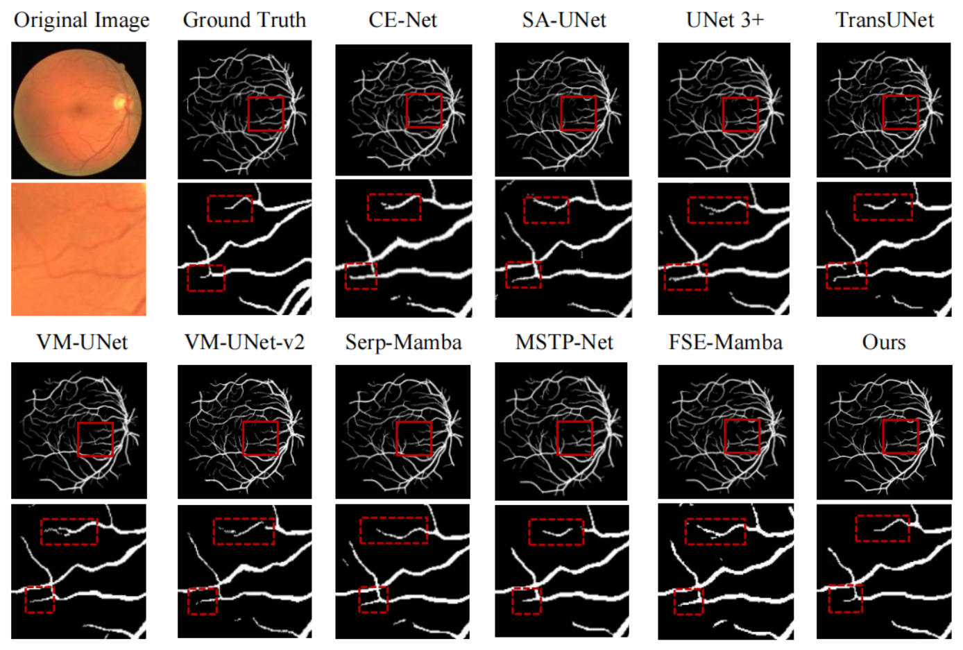
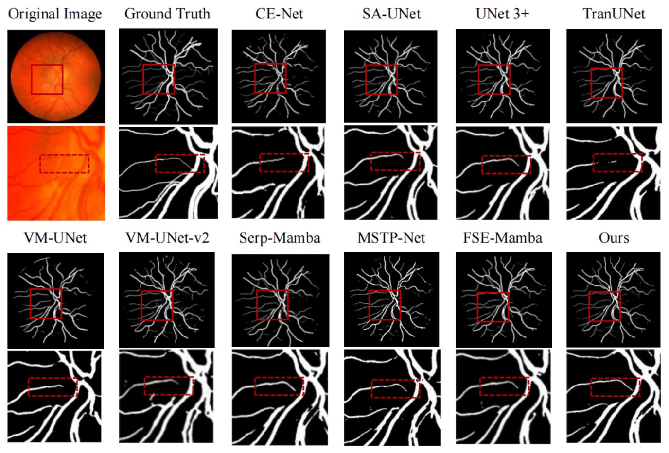
DatasetsSubjectsTraining/TestResolution
DRIVE [47]4020/20 584 × 565
CHASE_DB1 [48]2820/8 999 × 960
STARE [49]2010/10 700 × 605
IOSTAR [50]3025/5 1024 × 1024
Table 3. Detailed configurations of experimental settings and network components for the proposed FDPR-DBNet.
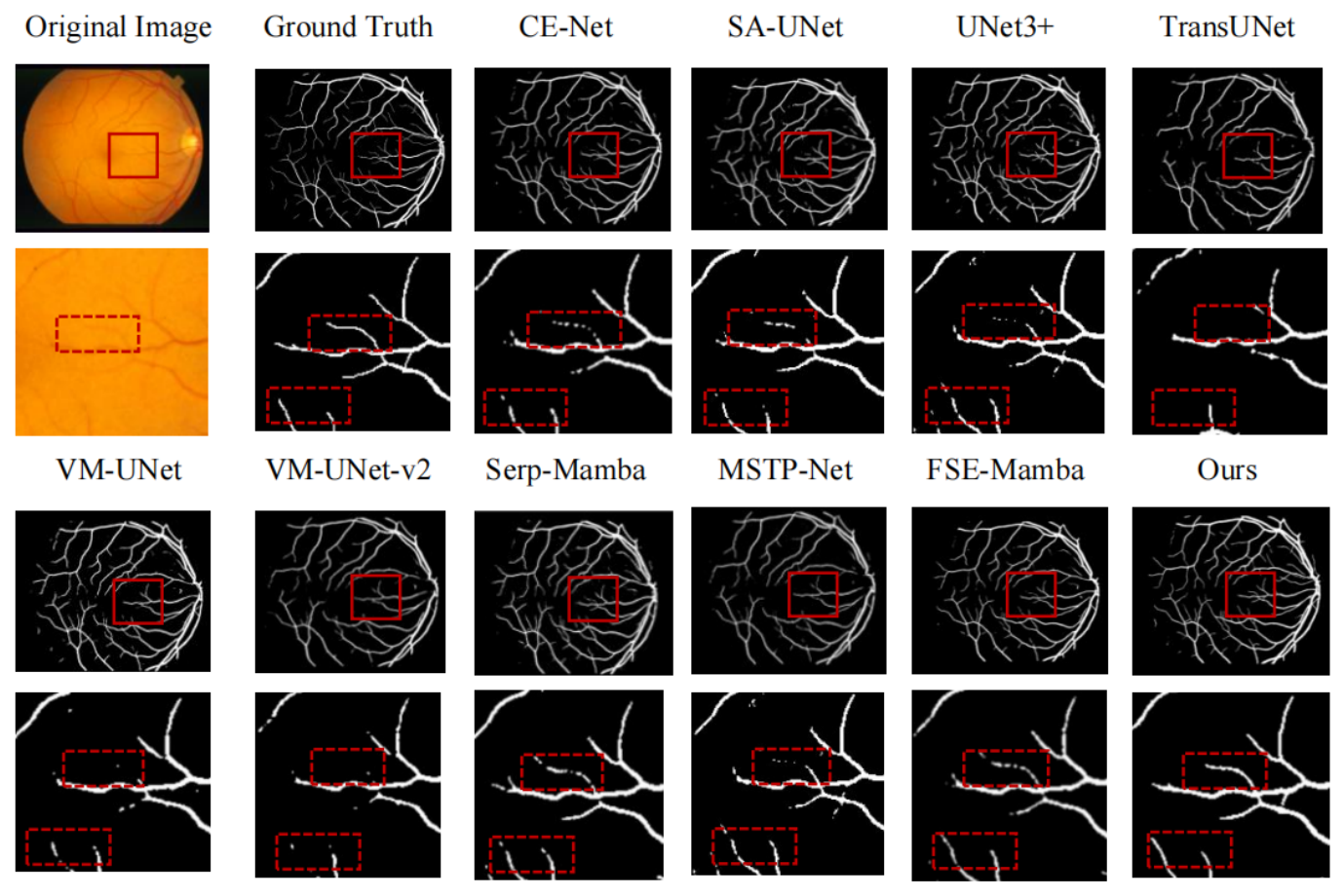
CategoryFunctionality/Parameter TypeParameter/Value
Experimental Settings
Hardware & OSComputing Platform2× NVIDIA GeForce RTX 4070Ti (12 GB each), Ubuntu 20.04
Software EnvironmentLanguage & FrameworkPython 3.10, PyTorch 2.0
Training SettingsParameters & ScaleInput size: 512 × 512 , Epochs: 100, Batch size: 8
OptimizationOptimizer & ScheduleAdam Optimizer, CosineAnnealingLR scheduler, Initial learning rate: 10 4 , Weight decay: 10 4
Loss FunctionBalanceWeight balance factor λ = 1
Pre-/post-processingAugmentation & InferenceCLAHE (for data augmentation), No post-processing
Network Components
DWTFrequency DecompositionHaar Wavelet (parameter-free), 1-level 2D decomposition (symmetric padding), Scale_factor = 0.5, LL sub-band for low-frequency branch, {LH, HL, HH} for high-frequency branch (both followed by separate 1 × 1 convolutions for channel projection to C)
SFCAFeature ActivationMulti-scale Pooling ( 1 × 1 , 2 × 2 , 3 × 3 ), SSM ( d state = 16 for S6), FFT/IFFT, LeakyReLU (negative slope α = 0.2 )
PACAFeature ActivationParallel Atrous Conv ( k = 3 , s = 1 ) with dilation rates r { 1 , 2 , 5 } , LeakyReLU (negative slope α = 0.2 )
SARFSpatial-Residual FusionDWConv ( k = 3 , s = 1 ), Residual Space Attention Conv ( k = 7 , s = 1 )
LDELocal Detail EnhancementInput local feature pyramid (2 or 3 levels), Window_Size = 8 × 8 , Multi-Head Attention (num_heads  = 4 , dim = 32 ), MLP ratio = 2
GSEGlobal Context ModelingInput global feature pyramid (4 levels), Multi-Head Attention (num_heads  = 4 , dim = 32 ), MLP ratio = 2
MPCRPrototype RefinementBilinear upsampling (Scale_factor  = 2 , align_corners  = True ), Conv ( k = 3 , s = 1 )
DConv BlockResolution RestorationBilinear upsampling (Scale_factor  = 2 , align_corners  = True ), Channel-wise concatenation, Conv ( k = 3 , s = 1 )
Table 4. Comparison with various methods on the DRIVE dataset. Bold denoted the best result; Underline denoted the second best.
Methods ACC (%) SE (%) SP (%) PR (%) AUC (%) MCC (%) Dice (%) clDice (%)
U-Net 95.56 ± 2.35 75.83 ± 1.17 96.08 ± 1.77 75.04 ± 2.01 97.89 ± 0.76 71.69 ± 3.45 75.43 ± 2.12 72.19 ± 3.85
CE-Net 96.71 ± 1.36 77.53 ± 1.29 97.31 ± 1.56 80.12 ± 2.77 97.42 ± 1.03 74.08 ± 2.68 78.80 ± 3.07 73.87 ± 3.29
LadderNet 97.18 ± 2.09 80.16 ± 3.34 98.07 ± 0.96 75.48 ± 1.97 97.36 ± 0.95 75.19 ± 1.36 77.75 ± 1.93 72.72 ± 4.11
SA-UNet 96.13 ± 1.78 77.20 ± 0.95 98.02 ± 0.88 81.37 ± 1.39 98.10 ± 0.78 77.10 ± 1.45 79.23 ± 1.32 75.73 ± 2.16
UNet3+ 96.60 ± 2.45 77.84 ± 1.66 97.55 ± 1.65 78.28 ± 3.25 98.23 ± 1.02 75.71 ± 4.21 78.06 ± 3.17 73.88 ± 3.19
TransUNet 96.43 ± 3.11 79.83 ± 1.58 97.80 ± 1.31 77.04 ± 2.43 97.51 ± 0.93 76.41 ± 3.17 78.41 ± 2.25 71.26 ± 3.44
VM-UNet 97.28 ± 1.93 78.91 ± 2.35 97.22 ± 0.75 77.58 ± 2.32 97.82 ± 1.02 76.61 ± 2.39 78.24 ± 3.83 73.26 ± 3.26
VM-UNet-v2 96.03 ± 1.58 79.02 ± 1.94 97.97 ± 0.37 78.90 ± 2.04 97.88 ± 0.97 77.04 ± 1.94 78.96 ± 2.98 74.23 ± 2.78
Serp-Mamba 97.45 ± 0.97 83.12 ± 1.93 98.67 ± 0.42 84.56 ± 1.58 98.32 ± 0.74 81.93 83.83 ± 1.33 78.93 ± 2.12
MSTP-Net 97.17 ± 1.52 80.33 ± 2.19 98.11 ± 0.49 81.04 ± 2.12 98.01 ± 0.47 78.84 ± 3.42 80.68 ± 3.63 77.83 ± 3.69
PA-Net 95.82 82.84 98.07 85.04 98.33 83.93
FreqUNet 98.31 81.85 98.12 97.00 75.82
FSE-Mamba 97.72 ± 1.37 80.51 ± 2.33 98.73 ± 0.22 81.87 ± 2.51 98.31 ± 0.37 79.86 ± 3.82 81.18 ± 2.19 78.87 ± 2.54
MSCR-Net 97.07 83.41 98.40 98.91 83.21
SDHM2T 96.9676.7698.3198.79 77.30 82.90
CRMA-UNet 97.21 84.6298.8583.93
Ours97.75 ± 1.09 87.21 ± 0.36 98.80 ± 0.18 85.74 ± 1.36 98.43 ± 0.26 85.32 ± 2.18 86.47 ± 1.33 80.19 ± 2.11
Table 5. Comparison with various methods on the CHASE_DB1 dataset. Bold denoted the best result; Underline denoted the second best.
Methods ACC (%) SE (%) SP (%) PR (%) AUC (%) MCC (%) Dice (%) clDice (%)
U-Net 95.01 ± 1.92 80.85 ± 1.38 96.77 ± 1.36 69.79 ± 2.02 97.08 ± 1.43 73.11 ± 3.21 74.92 ± 2.26 69.33 ± 3.54
CE-Net 96.45 ± 2.16 76.64 ± 2.45 97.23 ± 1.22 79.53 ± 1.87 97.44 ± 0.94 75.02 ± 1.87 78.06 ± 2.97 74.23 ± 3.61
LadderNet 96.61 ± 1.01 79.26 ± 2.96 97.34 ± 0.78 77.08 ± 1.36 97.63 ± 0.82 74.71 ± 1.74 78.15 ± 1.37 72.44 ± 3.65
SA-UNet 97.38 ± 0.98 78.40 ± 1.38 97.65 ± 1.01 79.65 ± 2.08 98.12 ± 0.31 76.82 ± 1.72 79.02 ± 0.86 76.24 ± 3.01
UNet3+ 96.36 ± 2.33 76.40 ± 1.42 97.15 ± 1.44 76.78 ± 2.93 96.94 ± 2.86 73.73 ± 2.46 76.59 ± 3.23 72.76 ± 2.59
TransUNet 96.03 ± 2.76 80.71 ± 1.51 97.28 ± 0.86 78.43 ± 1.89 97.78 ± 1.04 77.02 ± 2.52 79.55 ± 1.95 73.22 ± 3.39
VM-UNet 96.81 ± 1.28 76.77 ± 1.97 97.23 ± 1.24 77.83 ± 1.36 98.10 ± 0.78 74.44 ± 1.82 77.30 ± 3.06 74.08 ± 2.73
VM-UNet-v2 95.76 ± 1.87 79.56 ± 0.69 97.68 ± 0.77 77.17 ± 2.91 98.32 ± 0.52 76.19 ± 2.33 78.35 ± 2.47 75.42 ± 3.01
Serp-Mamba 97.82 ± 1.01 84.35 ± 1.38 98.81 ± 0.25 83.12 ± 2.06 98.35 ± 0.33 82.59 ± 2.59 83.73 ± 1.95 79.23 ± 2.19
MSTP-Net 97.30 ± 1.78 81.87 ± 1.42 98.10 ± 0.71 80.32 ± 2.31 98.18 ± 0.28 79.28 ± 2.95 81.09 ± 2.06 78.84 ± 1.86
PA-Net 96.77 85.70 97.79 80.61 98.75 83.08
FreqUNet 97.86 81.86 98.44 81.37 98.00 77.23
FSE-Mamba 97.23 ± 1.62 80.78 ± 1.96 98.51 ± 0.53 81.37 ± 1.76 98.41 ± 0.82 78.91 ± 3.25 81.07 ± 2.36 78.26 ± 2.72
MSCR-Net 97.64 84.38 98.55 99.10 81.89
SDHM2T 97.48 86.83 98.00 98.93 80.16 81.30
CRMA-UNet 97.98 85.86 98.9285.80
Ours98.19 ± 0.76 86.35 ± 1.42 98.63 ± 0.13 84.77 ± 1.06 98.66 ± 0.74 82.31 ± 1.97 85.55 ± 1.21 81.08 ± 1.55
Table 6. Comparison with various methods on the STARE dataset. Bold denoted the best result; Underline denoted the second best.
Methods ACC (%) SE (%) SP (%) PR (%) AUC (%) MCC (%) Dice (%) clDice (%)
U-Net 96.02 ± 1.88 74.28 ± 2.32 97.19 ± 1.09 72.36 ± 3.27 97.13 ± 1.12 70.71 ± 3.62 73.30 ± 1.94 68.43 ± 3.21
CE-Net 96.91 ± 1.79 72.56 ± 2.12 97.69 ± 0.74 74.26 ± 2.33 98.31 ± 0.65 70.92 ± 2.54 73.40 ± 2.18 69.31 ± 1.73
LadderNet 96.83 ± 2.04 73.75 ± 3.11 97.96 ± 1.02 74.55 ± 2.42 98.22 ± 0.49 72.33 ± 1.92 74.15 ± 3.41 71.22 ± 2.57
SA-UNet 97.17 ± 0.92 78.77 ± 1.24 98.57 ± 0.52 79.50 ± 1.87 98.02 ± 1.21 68.87 ± 1.35 79.13 ± 1.13 77.32 ± 2.62
UNet3+ 97.56 ± 2.03 74.46 ± 2.60 96.37 ± 1.64 72.39 ± 2.35 97.33 ± 1.19 76.63 ± 2.76 73.41 ± 2.02 68.49 ± 3.35
TransUNet 96.56 ± 1.98 77.00 ± 1.44 97.55 ± 1.17 76.41 ± 2.88 97.07 ± 1.95 74.22 ± 3.07 76.70 ± 2.44 72.68 ± 2.42
VM-UNet 97.01 ± 1.75 76.87 ± 2.51 97.13 ± 1.23 76.89 ± 1.94 96.15 ± 2.04 74.01 ± 2.74 76.88 ± 3.12 74.16 ± 2.93
VM-UNet-v2 97.95 ± 0.52 78.83 ± 1.37 97.48 ± 0.52 77.14 ± 2.75 97.12 ± 1.86 75.68 ± 2.45 77.97 ± 2.88 73.95 ± 2.86
Serp-Mamba 97.58 ± 1.76 86.94 ± 1.62 98.42 ± 0.48 85.26 ± 1.82 98.41 ± 0.16 84.32 ± 1.79 86.09 ± 1.65 80.52 ± 1.91
MSTP-Net 97.87 ± 0.82 78.39 ± 2.25 98.00 ± 1.12 79.55 ± 1.96 98.17 ± 0.42 76.94 ± 3.02 78.97 ± 2.56 77.53 ± 3.42
PA-Net 97.07 88.13 98.05 83.23 99.08 85.61
FreqUNet 96.86 74.28 98.01 95.00 67.21
FSE-Mamba 97.88 ± 1.08 84.01 ± 2.11 98.37 ± 0.76 81.26 ± 2.14 98.55 ± 0.78 81.32 ± 2.98 82.61 ± 1.87 79.76 ± 3.02
MSCR-Net 97.83 84.44 98.7499.28 83.10
SDHM2T 97.53 83.26 98.70 99.03 82.15 83.27
CRMA-UNet 97.98 87.37 97.64 82.27
Ours98.16 ± 0.93 88.12 ± 1.33 99.02 ± 0.21 84.61 ± 2.13 98.70 ± 0.38 84.76 ± 2.03 86.33 ± 1.07 81.54 ± 1.64
Table 7. Comparison with various methods on the IOSTAR dataset. Bold denoted the best result; Underline denoted the second best.
Methods ACC (%) SE (%) SP (%) PR (%) AUC (%) MCC (%) Dice (%) clDice (%)
U-Net 95.85 ± 2.17 69.34 ± 3.10 97.56 ± 1.19 79.12 ± 3.08 97.49 ± 1.32 70.89 ± 2.91 73.91 ± 1.98 70.89 ± 2.74
CE-Net 97.32 ± 1.73 80.88 ± 1.98 96.42 ± 1.88 77.42 ± 2.98 98.03 ± 1.08 75.94 ± 2.59 79.11 ± 2.11 72.53 ± 1.86
LadderNet 96.81 ± 1.84 76.66 ± 2.39 97.24 ± 1.24 75.67 ± 2.81 97.09 ± 1.73 73.40 ± 2.86 76.16 ± 2.42 71.89 ± 3.07
SA-UNet 98.90 ± 0.63 75.83 ± 1.22 98.25 ± 0.74 76.98 ± 1.62 98.17 ± 0.52 74.98 ± 1.09 76.40 ± 2.56 76.34 ± 2.71
UNet3+ 96.91 ± 2.48 69.12 ± 3.25 98.11 ± 0.65 80.01 ± 2.14 97.11 ± 1.70 72.17 ± 2.33 74.17 ± 2.28 69.57 ± 2.79
TransUNet 97.37 ± 1.76 73.77 ± 2.59 97.58 ± 1.46 81.01 ± 1.88 97.35 ± 1.44 74.33 ± 2.69 77.22 ± 3.47 73.81 ± 3.92
VM-UNet 97.01 ± 1.89 75.19 ± 2.36 98.14 ± 0.55 79.90 ± 2.45 98.27 ± 0.28 75.61 ± 2.95 77.47 ± 2.90 75.62 ± 3.04
VM-UNet-v2 96.12 ± 1.08 76.99 ± 2.08 96.62 ± 1.58 78.21 ± 2.28 96.39 ± 1.73 74.11 ± 3.18 77.59 ± 2.42 76.57 ± 3.77
Serp-Mamba 97.12 ± 1.31 80.96 ± 2.10 98.43 ± 0.35 84.91 ± 1.83 98.08 ± 0.28 81.19 ± 2.25 82.89 ± 2.41 81.44 ± 2.65
MSTP-Net 97.02 ± 1.28 81.86 ± 1.58 98.34 ± 1.02 81.08 ± 1.88 98.21 ± 0.74 79.88 ± 3.21 81.47 ± 1.79 79.85 ± 2.07
FSE-Mamba 97.44 ± 2.21 82.51 ± 1.82 98.05 ± 1.08 83.75 ± 1.95 98.32 ± 0.78 81.73 ± 2.03 83.13 ± 1.96 81.94 ± 2.98
SDHM2T 97.33 81.93 98.6898.76 81.54 82.86
CRMA-UNet 97.56 89.43 98.67 84.67
Ours97.61 ± 1.09 86.69 ± 1.72 98.75 ± 0.28 84.21 ± 2.01 98.37 ± 0.41 84.31 ± 1.71 85.43 ± 0.79 82.70 ± 2.32
Table 8. Cross-dataset generalization comparison of different methods trained on the STARE dataset and tested on the DRIVE and CHASE_DB1 datasets. Bold denoted the best result; Underline denoted the second best.
Methods STARE → DRIVE STARE → CHASE_DB1
ACC (%)SE (%)SP (%)PR (%)Dice (%)AUC (%)ACC (%)SE (%)SP (%)PR (%)Dice (%)AUC (%)
SA-UNet 96.44 77.61 97.12 80.19 78.88 97.35 95.55 75.39 95.91 77.53 76.45 96.70
TransUNet 96.59 80.28 97.54 76.58 78.39 97.83 96.34 78.34 96.66 78.10 78.22 97.46
Serp-Mamba 97.3281.25 98.73 81.92 81.58 98.20 97.05 83.7898.58 80.52 82.1297.97
MSTP-Net 96.23 78.63 97.61 81.31 79.92 96.46 95.31 76.27 96.30 76.32 76.29 96.89
FSE-Mamba 97.17 79.34 98.28 83.19 81.22 98.4898.02 83.25 97.48 79.51 81.34 97.23
CRMA-UNet 97.10 80.79 98.7481.94
Ours 97.2986.4098.9485.1385.7598.3198.3485.32 97.34 83.2484.2798.22
Table 9. Cross-dataset generalization comparison of different methods trained on the CHASE_DB1 dataset and tested on DRIVE and STARE datasets. Bold denoted the best result; Underline denoted the second best.
Methods CHASE_DB1 → DRIVE CHASE_DB1 → STARE
ACC (%)SE (%)SP (%)PR (%)Dice (%)AUC (%)ACC (%)SE (%)SP (%)PR (%)Dice (%)AUC (%)
SA-UNet 95.89 75.46 96.32 76.56 76.01 96.45 96.47 74.29 95.68 78.45 76.31 97.59
TransUNet 96.45 77.78 96.21 76.48 77.12 98.06 96.81 76.64 97.36 74.36 75.48 96.03
Serp-Mamba 96.11 80.7997.2879.5480.16 97.68 97.06 81.34 95.43 79.95 80.64 97.67
MSTP-Net 96.36 78.45 96.78 76.98 77.71 97.52 95.78 76.04 96.32 75.34 75.69 95.23
FSE-Mamba 97.15 78.43 97.14 78.30 78.30 97.79 96.14 82.57 97.35 81.4582.0197.78
Ours 96.8883.2997.4882.2582.7698.1297.2384.68 96.67 80.3482.4398.14
Table 10. Cross-dataset generalization comparison of different methods trained on the DRIVE dataset and tested on the STARE and CHASE_DB1 datasets. Bold denoted the best result; Underline denoted the second best.
Methods DRIVE → STARE DRIVE → CHASE_DB1
ACC (%)SE (%)SP (%)PR (%)Dice (%)AUC (%)ACC (%)SE (%)SP (%)PR (%)Dice (%)AUC (%)
SA-UNet 96.31 77.93 97.15 75.32 76.60 97.32 95.79 76.31 95.69 76.89 76.60 95.55
TransUNet 98.54 80.32 97.42 74.21 77.16 97.40 97.51 78.84 96.36 76.51 77.66 96.34
Serp-Mamba 96.46 82.48 98.32 80.36 81.41 98.23 96.92 79.63 97.45 77.94 78.78 97.05
MSTP-Net 95.35 80.72 96.89 76.54 78.36 96.78 93.78 75.22 95.56 78.53 76.84 95.31
FSE-Mamba 97.93 83.37 97.72 81.79 82.57 97.39 97.81 80.35 97.02 79.80 80.07 98.02
CRMA-UNet 95.90 88.98 96.51 75.82
Ours 96.32 87.3498.4582.0884.6398.60 96.48 82.0197.2382.7782.3998.56
Table 11. Results of the ablation study on the DRIVE dataset. Bold denoted the best result.
MethodsACC
(%)
SE
(%)
SP
(%)
PR
(%)
AUC
(%)
Dice
(%)
clDice
(%)
Params
(M)
FLOPs
(G)
FPS
(frames/s)
Baseline95.5974.3297.8478.8397.5776.5167.34 1.85 2.14 95.33
High frequency95.2274.2497.1377.9797.6976.0667.42 2.02 2.41 92.15
Low frequency96.0176.2297.8078.5097.8077.3469.33 2.08 2.83 91.80
+DbE (CFF)96.3880.5198.0781.7998.2381.1574.68 2.43 3.05 87.45
+DbE + SARF97.1182.1398.8281.2498.2481.6876.50 2.68 3.58 85.10
+DbE + SARF + LDE97.3583.8198.0783.1198.1483.4677.67 3.05 4.35 82.30
+DbE + SARF + CSE (GSE + LDE)97.4585.2798.2384.7698.4185.0179.68 3.48 5.12 79.04
+DbE + SARF + CSE + MPCR97.7587.2198.8085.7598.4386.4780.19 3.73 5.67 78.18
Table 12. Ablation study of different frequency and feature fusion variants. Bold denoted the best result.
MethodsACC (%)SE (%)SP (%)PR (%)Dice (%)AUC (%)
DbE96.3880.5198.0781.7981.1598.23
+Add96.4080.4398.2280.0480.2398.44
+CBAM96.7581.1898.1281.2381.2097.87
+Residual Fusion96.6181.9898.4680.2281.0998.19
Proposed (+SARF)97.1182.1398.8281.2481.6898.24
Table 13. Comparison with other loss functions on the DRIVE dataset. Bold denoted the best result; Underline denoted the second best.
Methods ACC (%) SE (%) SP (%) PR (%) AUC (%) Dice (%) clDice (%)
Backbone + clDice Loss 96.26 86.51 97.19 83.90 98.12 85.1879.87
Backbone + BettiLoss 96.12 85.33 96.24 84.05 97.24 84.69 77.63
Backbone + TopoLoss 97.67 83.64 98.63 81.64 98.45 82.63 76.76
Backbone + L c 97.7587.2197.8085.7598.4386.4780.19
Table 14. p-values between the proposed model and various methods on the DRIVE and CHASE_DB1 datasets.
Methods ACC SE SP PR AUC MCC Dice clDice
DRIVE
U-Net 0.095 <0.001 0.009 0.001 0.171 <0.001 <0.001 0.004
CE-Net 0.219 <0.001 0.067 0.004 0.066 <0.001 0.001 0.007
LadderNet 0.603 0.002 0.133 <0.001 0.041 <0.001 <0.001 0.007
SA-UNet 0.121 <0.001 0.088 0.001 0.396 <0.001 <0.001 0.011
UNet3+ 0.366 <0.001 0.131 0.002 0.682 0.002 <0.001 0.006
TransUNet 0.397 <0.001 0.129 <0.001 0.066 0.001 <0.001 0.001
VM-UNet 0.648 <0.001 0.002 <0.001 0.231 <0.001 0.002 0.004
VM-UNet-v2 0.080 <0.001 0.002 <0.001 0.256 <0.001 0.001 0.005
Serp-Mamba 0.658 0.002 0.542 0.241 0.762 0.091 0.014 0.374
MSTP-Net 0.508 <0.001 0.018 0.003 0.119 0.007 0.010 0.250
FSE-Mamba 0.970 <0.001 0.597 0.016 0.569 0.024 0.002 0.298
CHASE_DB1
U-Net 0.009 <0.001 0.016 <0.001 0.060 <0.001 <0.001 <0.001
CE-Net 0.128 <0.001 0.034 <0.001 0.052 <0.001 <0.001 0.005
LadderNet 0.023 0.001 0.007 <0.001 0.071 <0.001 <0.001 0.001
SA-UNet 0.182 <0.001 0.064 0.001 0.171 0.002 <0.001 0.013
UNet3+ 0.134 <0.001 0.051 <0.001 0.229 <0.001 <0.001 <0.001
TransUNet 0.130 <0.001 0.008 <0.001 0.162 0.006 <0.001 0.002
VM-UNet 0.072 <0.001 0.036 <0.001 0.278 <0.001 <0.001 0.001
VM-UNet-v2 0.027 <0.001 0.026 <0.001 0.425 0.002 <0.001 0.006
Serp-Mamba 0.531 0.054 0.191 0.150 0.417 0.852 0.114 0.162
MSTP-Net 0.334 0.001 0.139 0.004 0.212 0.093 0.003 0.072
FSE-Mamba 0.265 <0.001 0.636 0.006 0.626 0.080 0.005 0.079
Table 15. p-values between the proposed model and various methods on the STARE and IOSTAR datasets.
Methods ACC SE SP PR AUC MCC Dice clDice
STARE
U-Net 0.052 <0.001 0.006 <0.001 0.018 <0.001 <0.001 <0.001
CE-Net 0.203 <0.001 0.005 <0.001 0.280 <0.001 <0.001 <0.001
LadderNet 0.221 <0.001 0.052 <0.001 0.122 <0.001 <0.001 <0.001
SA-UNet 0.129 <0.001 0.111 0.004 0.265 <0.001 <0.001 0.016
UNet3+ 0.565 <0.001 0.007 <0.001 0.040 0.002 <0.001 <0.001
TransUNet 0.141 <0.001 0.024 <0.001 0.104 <0.001 <0.001 <0.001
VM-UNet 0.231 <0.001 0.010 <0.001 0.025 <0.001 <0.001 0.001
VM-UNet-v2 0.671 <0.001 <0.001 0.001 0.100 <0.001 <0.001 <0.001
Serp-Mamba 0.533 0.244 0.034 0.618 0.154 0.726 0.792 0.391
MSTP-Net 0.615 <0.001 0.080 0.004 0.070 0.001 <0.001 0.046
FSE-Mamba 0.672 0.006 0.103 0.038 0.709 0.065 0.005 0.280
IOSTAR
U-Net 0.143 <0.001 0.061 0.015 0.192 <0.001 <0.001 <0.001
CE-Net 0.759 0.001 0.025 0.003 0.529 <0.001 <0.001 <0.001
LadderNet 0.426 <0.001 0.029 <0.001 0.146 <0.001 <0.001 <0.001
SA-UNet 0.050 <0.001 0.195 <0.001 0.518 <0.001 <0.001 0.004
UNet3+ 0.579 <0.001 0.078 0.013 0.146 <0.001 <0.001 <0.001
TransUNet 0.802 <0.001 0.116 0.032 0.166 <0.001 <0.001 0.002
VM-UNet 0.555 <0.001 0.058 0.016 0.664 <0.001 <0.001 0.003
VM-UNet-v2 0.061 <0.001 0.018 0.002 0.038 <0.001 <0.001 0.015
Serp-Mamba 0.537 0.002 0.149 0.581 0.228 0.039 0.055 0.447
MSTP-Net 0.454 0.002 0.411 0.035 0.684 0.026 0.002 0.075
FSE-Mamba 0.881 0.006 0.198 0.723 0.902 0.061 0.041 0.665
Table 16. Comparison of computational complexity and performance. The metrics included parameter count, Training Memory, Training Time per Epoch, Inference Memory, Inference Time per Case, FPS, FLOPs, and Dice coefficient on the DRIVE dataset.
MethodsParams (M) Training Memory (GB) Training Time per Epoch (s) Inference Memory (MB) Inference Time per Case (ms) FPS (frames/s) FLOPs (G)Dice (%)
U-Net7.76 3.68 7.19 8.61 10.86 92.11 4.0575.43
CE-Net29.00 6.21 12.23 43.62 16.61 60.22 2.8878.80
LadderNet2.88 4.19 6.59 12.97 15.34 65.19 2.1977.75
SA-UNet1.16 4.72 7.43 6.42 11.28 88.64 0.8879.23
UNet3+26.97 8.55 18.77 98.69 45.35 22.05 79.5478.06
TransUNet67.87 11.39 24.31 238.91 21.99 45.47 14.7678.41
VM-UNet29.77 6.91 17.63 94.55 30.09 33.23 17.1278.24
VM-UNet-v222.27 5.17 16.55 89.94 27.09 36.92 12.1678.96
Serp-Mamba22.45 5.95 16.98 85.63 78.37 12.76 18.7283.83
MSTP-Net26.09 4.56 9.78 109.52 19.79 50.54 19.1180.68
FreqUNet0.26 - - - - - 1.4075.82
FSE-Mamba25.50 6.11 10.42 97.28 15.97 62.62 6.3281.18
Ours3.73 4.89 8.01 15.44 12.79 78.18 5.6786.47
Disclaimer/Publisher’s Note: The statements, opinions and data contained in all publications are solely those of the individual author(s) and contributor(s) and not of MDPI and/or the editor(s). MDPI and/or the editor(s) disclaim responsibility for any injury to people or property resulting from any ideas, methods, instructions or products referred to in the content.