Article

A Sign-Symmetric Reformulation of the Hassanat Distance for Data with Negative Feature Values
by
Mohammad Saad Alaydaa
1,
Gaseb N. Alotibi
1,
Ahmad S. Tarawneh
2 and
Ahmad B. Hassanat
2,*
1
Faculty of Computers and Information Technology, University of Tabuk, Tabuk 71491, Saudi Arabia
2
Faculty of Information Technology, Mutah University, Karak 61710, Jordan
*
Author to whom correspondence should be addressed.
Symmetry 2026, 18(7), 1225; https://doi.org/10.3390/sym18071225
Submission received: 18 June 2026 / Revised: 11 July 2026 / Accepted: 13 July 2026 / Published: 20 July 2026
(This article belongs to the Section B: Mathematics)

Abstract

The Hassanat Distance (HasD) is a bounded, non-convex metric widely used in k-nearest-neighbor (KNN) classification for its robustness to noise, outliers, and heterogeneous feature scales. Its definition, however, breaks a natural symmetry: through a sign-dependent shift it assigns different distances to mirror-image pairs such as ( 1 , 2 ) and ( 1 , 2 ) , distorting neighborhoods exactly in the value ranges that modern preprocessing (z-scoring, principal component analysis (PCA), learned embeddings) produces. We introduce the Sign-Symmetric Hassanat Distance (SHasD), a single branch-free formula D ( a , b ) = | a b | / ( 1 + max ( | a | , | b | ) ) that is invariant under the reflection x x , coincides exactly with HasD on non-negative data, and removes the conditional shift entirely. We prove SHasD is a metric, and we derive a range-normalized companion, SHasD-R, that additionally restores ray monotonicity and the [ 0 , 1 ) per-dimension bound. On 23 datasets across three normalization regimes and ten distance measures, SHasD improves significantly on HasD on data containing negative values (mean gain + 1.1 percentage points, up to + 7.4 ; Wilcoxon p = 0.0026 , Holm-corrected) and attains the best mean rank of the compared measures on signed, heavy-tailed, outlier-rich data, while preserving HasD’s robustness. An additive per-dimension decomposition yields a built-in interpretation of every prediction.

1. Introduction

Distance measures are at the core of similarity-based learning. The k-nearest-neighbor (KNN) classifier [1,2] delegates all of its inductive bias to the chosen distance, and a large body of work shows that this choice materially affects accuracy and robustness [3,4,5]. Conventional metrics such as the Euclidean and Manhattan distances are sensitive to feature scale and to outliers: a single feature with a large range, or a single corrupted value, can dominate the sum. Robust distance-based learning is an active concern well beyond standard KNN classification: outlier-aware methods explicitly account for corrupted or extreme observations, as in the iterative minimum-spanning-tree detector of Li et al. for medical data [6]; fault-diagnosis systems build multilabel classifiers on feature fusion and fault-similarity measures [7]; clustering algorithms adapt neighborhood graphs to heterogeneous density, where the distance shapes the graph itself [8]; and weighted classifiers model attribute and instance importance directly [9]. In all of these settings the behavior of the underlying distance or similarity on realistic—signed, standardized, outlier-contaminated—features is a first-order design concern.
There is also a mathematical motivation for designing new distance functions that is independent of any particular classifier. Whether a proposed dissimilarity satisfies the metric axioms, what topology it induces, whether it is complete, and which normalizations preserve these properties determine where the function can be deployed safely: metric indexing structures require triangle inequality, convergence arguments require completeness, and fixed-point machinery requires knowing the underlying (possibly generalized) metric structure [5,10]. Part of our contribution is to settle these questions for the proposed reformulation (Section 5.4 and Section 5.5).
The Hassanat distance (HasD) [11] addresses this by normalizing each dimension independently with a ratio that is bounded in [ 0 , 1 ) , so that no attribute—and no single corrupted value—can dominate. HasD has since been used successfully across applications including EEG analysis, content-based image retrieval, face and gesture recognition, biometrics, cancer classification, and fraud detection; a recent review collected this evidence and simplified the original proof [12]. Large comparative studies found it to be the overall top performer among tens of distances for KNN and notably insensitive to noise [3]. Most recently, the Hassanat ratio has been adapted into a family of loss functions for binary classification (HasLoss) [13], whose symmetric max-based denominator parallels, in the loss domain, the symmetrization we pursue here for the distance itself.
This paper addresses a structural asymmetry of HasD on negative feature values. HasD handles negatives by shifting both arguments upward by the absolute value of the minimum, which guarantees a positive ratio but makes the distance depend on the pair in a way that is not symmetric around zero: mirrored pairs receive different distances (Section 4). We stress at the outset that this behavior violates no metric axiom—it is a modeling choice embedded in the original definition. What we propose is an alternative normalization that possesses an additional invariance (sign symmetry) while agreeing with HasD wherever the original was designed to operate. Negative values are not an edge case. They arise natively (signed sensors, returns, differences, wavelet and cepstral coefficients), and they are manufactured by the two most common preprocessing steps in modern pipelines: z-score standardization and projection methods such as principal component analysis (PCA) or learned embeddings, both of which produce zero-centered features that are negative roughly half the time.
  • Contributions.
  • We identify and characterize the reflection asymmetry of HasD on negative values, and we show that its negative branch collapses to a translation-invariant transform of | a b | , structurally different from its positive branch (Section 4).
  • We propose the Sign-Symmetric Hassanat Distance (SHasD), a single, branch-free formula that coincides exactly with HasD on non-negative inputs and is invariant under sign reflection. We prove it is a metric and analyze its properties, and we derive a range-normalized companion, SHasD-R, which is additionally monotone along rays and bounded in [ 0 , 1 ) per dimension (Section 5). We further show that both metrics induce the standard Euclidean topology on R m , have the same convergent and Cauchy sequences as the Euclidean metric, and are complete (Section 5.4), and we exhibit SHasD as the unique backward-compatible member of a general family of admissible sign-symmetric normalizations (Section 5.5).
  • We evaluate SHasD against HasD and seven other distance measures with KNN on 23 datasets covering four scenarios—natively negative features, PCA-projected real data, z-score- and [ 1 , 1 ] -normalized classics, and signed data with native heavy-tailed outliers (financial returns and contaminated generators)—including a k-sweep and noise/outlier robustness experiments (Section 6 and Section 7). SHasD improves significantly on HasD on the datasets with negative values, attains the best mean rank of the ten compared measures under native outliers, and it preserves HasD’s robustness.

2. Related Work

The choice of distance function is the dominant design decision in nearest-neighbor learning, and a sustained line of work has studied how to make it well [3,4]. Recent algorithmic advances include locally scaled kernels with confidence voting [14], direct optimization of the distance function for neighbor-based classifiers [15], comparative analyses of KNN variants for prediction tasks [16], joint optimization of variable selection and neighborhood size [17], and hyperparameter tuning that targets the F β score directly [18]. The Hassanat distance figures prominently in this literature: its behavior has been analyzed in connection with the k = n rule and dimension-aware neighbor selection [19], integrated in an enhanced KNN that combines G-metric reconstruction with a Gray Wolf Optimizer [20], and benchmarked against competing metrics on large software-effort-estimation data [21]. It has also been adapted to unsupervised settings through iterative clustering with training [22] and GPU implementations in order to lower the computational cost of neighbor search at scale [23].
Apart from algorithmic study, KNN and Hassanat distance appear in a surprisingly large number of application domains. In biomedicine, they support cancer-data classification with robust distance measures [24], epilepsy diagnosis [25], weighted-KNN disease diagnosis on clinical data [26], amebiasis testing via decision-tree learning and data mining [27], studies of normalization and distance choice for diabetes classification [28], and pandemic-era sentiment analysis [29]. In computer vision and pattern recognition they drive face-mask detection and recognition [30,31], hand-gesture recognition [32], image-quality assessment [33], and UAV-based anomaly detection for photovoltaic inspection [34]. Industrial and engineering applications include bearing-fault diagnosis from auto-encoder features [35], fault classification in distributed generation and smart grids [36,37], non-destructive produce grading [38], ultrasonic assessment of stabilized soils [39], and intelligent threshold prediction for mesh segmentation [40]. The same toolkit reaches telecommunications and networking—QoS routing in SDN-IoT [41], data gathering in underwater sensor networks [42], visible-light indoor positioning [43], and traffic-flow prediction [44]—as well as automatic modulation classification [45], financial and economic forecasting [46,47,48], hardware-security side-channel analysis [49], agricultural recommendation systems [50], and information-theoretic accounts of generalization [51]. Methodologically novel proximity notions also continue to appear, including p-adic distances for KNN [52] and weighted metrics coupled with three-way decision theory [53].
Two observations motivated the present work. First, the effectiveness of each of these systems is inseparable from the distance it uses, and the Hassanat distance is repeatedly singled out for its boundedness and robustness to noise and outliers [3,12,19]. Second, the great majority of these pipelines operate on data that is standardized, projected, or natively signed—exactly the regime in which the reflection asymmetry analyzed in Section 4 arises. A sign-symmetric reformulation that preserves HasD’s robustness therefore stands to benefit this entire body of applications without changing how it is deployed.
  • Position within generalized distance structures.
From a mathematical standpoint, the present construction belongs to the broader study of generalized and normalized distance structures, which we briefly situate. One long-standing line of research relaxes the metric axioms themselves: b-metric spaces weaken the triangle inequality by a multiplicative constant [54]; partial metric spaces permit nonzero self-distance [55]; metric-like (dislocated) spaces relax the identity of indiscernibles [56]; and fuzzy metric spaces, in the tradition of Kramosil–Michálek and George–Veeramani [57,58], replace numerical distances by degrees of nearness—see the recent survey of fixed-point results, contraction principles, and simulation functions in fuzzy metric spaces by Moussaoui and Radenović [10]. Perturbed and parametric metric constructions for distance modeling continue to appear in this literature [59]. A second line studies metric-preserving functions: transforms f d of an existing metric d that remain metrics, characterized by subadditivity-type conditions [60]; the bounded remetrizations d / ( 1 + d ) and min ( 1 , d ) are the classical examples. The Hassanat family fits neither frame exactly: it satisfies the classical metric axioms in full (no relaxation), yet it is not a metric-preserving transform of | a b | , because its normalizer depends on the pair ( a , b ) through max ( | a | , | b | ) rather than on the difference alone. It is precisely this pair-dependent, scale-adaptive normalization that produces the boundedness and outlier robustness prized in applications—and that requires the direct proofs of Section 5 in place of citable transform theorems. Section 5.5 makes the connection systematic by characterizing a family of admissible normalizers, and extending the sign-symmetric construction to b-metric or fuzzy settings is a natural direction we leave open (Section 9).

3. Background: The Hassanat Distance

For feature vectors p , q R m , HasD is defined as HasD ( p , q ) = i = 1 m D ( p i , q i ) with
D ( a , b ) = 1 1 + min ( a , b ) 1 + max ( a , b ) , min ( a , b ) 0 , 1 1 + min ( a , b ) + | min ( a , b ) | 1 + max ( a , b ) + | min ( a , b ) | , min ( a , b ) < 0 .
Each dimension contributes a value in [ 0 , 1 ) , reaching 1 only in the limit max (or min ), which yields HasD’s hallmark properties: boundedness per dimension, insensitivity to feature scale, and robustness to outliers [3,11,12].

4. The Problem: Reflection Asymmetry on Negative Values

Write the positive branch of (1) in ratio-free form:
1 1 + min ( a , b ) 1 + max ( a , b ) = max ( a , b ) min ( a , b ) 1 + max ( a , b ) = | a b | 1 + max ( a , b ) , a , b 0 .
The distance is the absolute difference, normalized by the magnitude of the larger value. Now consider the negative branch. Substituting s = | min ( a , b ) | gives 1 + min + s = 1 and 1 + max + s = 1 + max min , hence
D ( a , b ) = max ( a , b ) min ( a , b ) 1 + max ( a , b ) min ( a , b ) = | a b | 1 + | a b | , min ( a , b ) < 0 .
The negative branch therefore depends on the difference only: all information about the magnitudes of a and b is discarded. The two branches are structurally different normalizations, and the result is an asymmetry under reflection x x :
D ( 1 , 2 ) = 1 3 but D ( 1 , 2 ) = 1 2 , D ( 3 , 7 ) = 1 2 but D ( 3 , 7 ) = 4 5 .
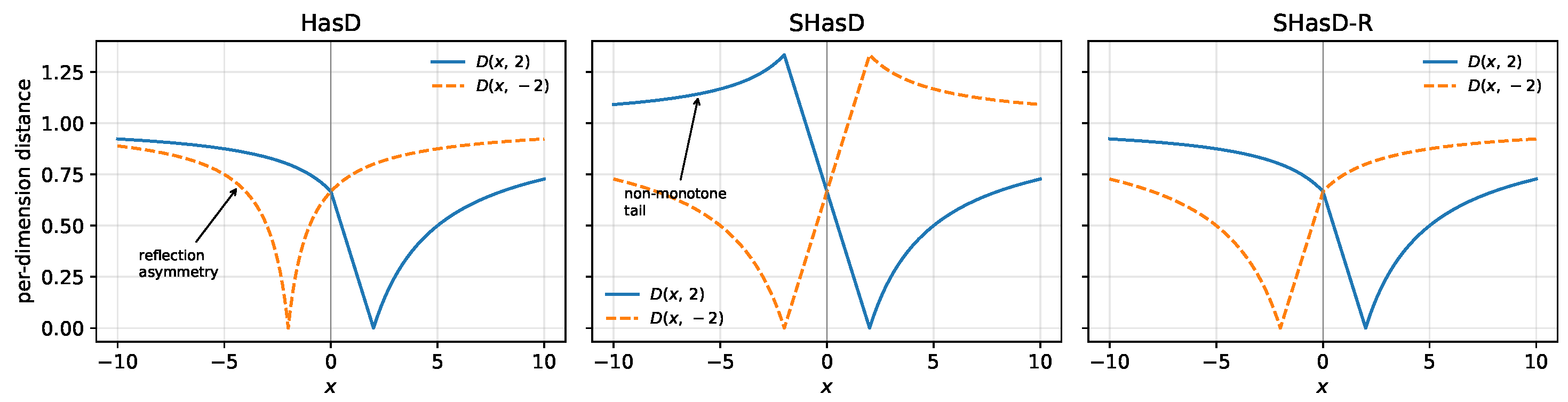
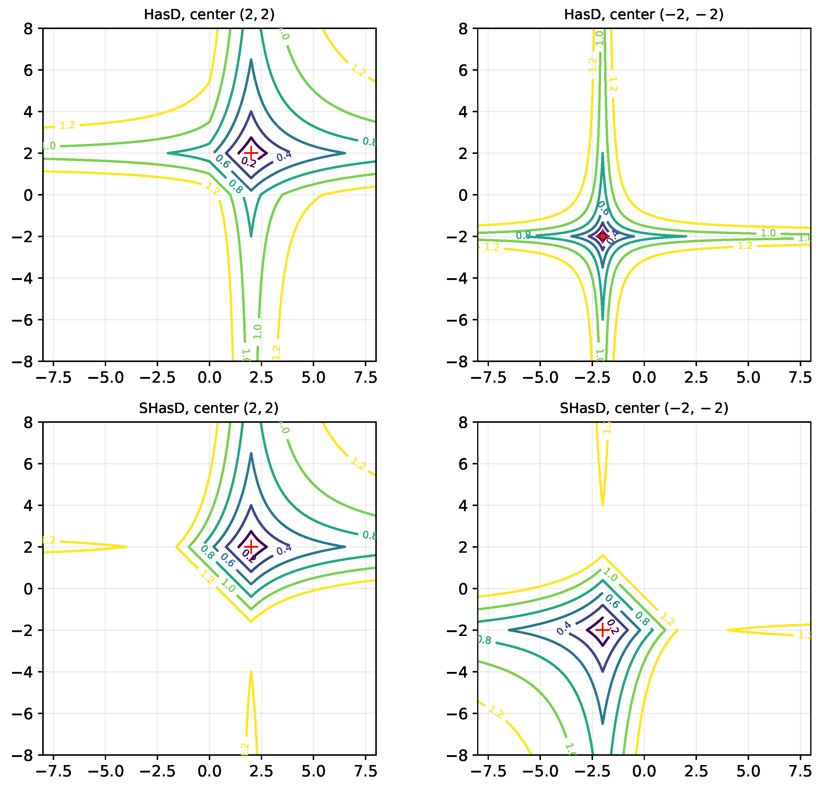
Mirrored pairs—identical configurations up to the sign convention of the measurement—receive different distances. Figure 1(left) visualizes the effect: the profile of D ( x , 2 ) is not the mirror image of D ( x , 2 ) . In a KNN neighborhood this means that the same geometric structure is judged differently on the negative side of a feature than on the positive side, and points whose features straddle zero have their neighborhoods distorted. We call this invariance under the reflection x x sign symmetry. It should not be confused with the symmetry axiom of a metric, d ( a , b ) = d ( b , a ) , which HasD satisfies; indeed, sign symmetry is not required by the metric axioms at all—HasD is a metric [11,12]. It is, however, a natural invariance to demand of a general-purpose distance on R m , where the sign convention of a feature (profit/loss, charge polarity, direction) is frequently arbitrary. Figure 2 visualizes the same asymmetry in two dimensions through the level sets of the summed per-dimension distance.

5. SHasD: A Sign-Symmetric, Branch-Free Reformulation

Equation (2) suggests the reformulation: keep the positive branch exactly, and extend the magnitude normalization to all reals through absolute values. We define, for  p , q R m ,
SHasD ( p , q ) = i = 1 m D s ( p i , q i ) , D s ( a , b ) = | a b | 1 + max | a | , | b | .
No case analysis, no shift term, and no division-line correction: a single expression on all of  R .
  • Notation.
Throughout the paper, D (1), D s (4), and  D r (5) denote the one-dimensional (per-dimension) distance functions, while HasD, SHasD, and SHasD-R denote the corresponding coordinate-sum metrics on R m . We use the symbols D, D s , D r only in mathematical statements about a single dimension; all figures, tables, and experimental discussion use the names HasD, SHasD, and SHasD-R uniformly.

5.1. Elementary Properties

Proposition 1
(Backward compatibility). For a , b 0 , D s ( a , b ) = D ( a , b ) , i.e., SHasD coincides with HasD on non-negative data.
Proof. 
For a , b 0 , max ( | a | , | b | ) = max ( a , b ) , and (2) shows the two expressions are equal.    □
  • Why was this not done before?
The reformulation is natural only in hindsight. The two-branch definition (1) conceals the structure: written as ratios of shifted minima and maxima, neither branch suggests a common closed form. Only when the positive branch is rewritten in the difference form (2)—a simplification introduced, for computational reasons, only recently [12]—do the magnitude-discarding nature of the negative branch (3) and the absolute-value extension become visible. Tellingly, even the most recent work to build directly on this non-convex ratio—using it to define an outlier-robust accuracy measure for machine-learning regression [61]—carries the original sign-dependent treatment of negative values unchanged, evidence that the reflection asymmetry had gone unnoticed rather than been weighed and deliberately accepted.
Proposition 2
(Sign symmetry). D s ( a , b ) = D s ( a , b ) for all a , b R ; consequently SHasD ( p , q ) = SHasD ( p , q ) .
Proof. 
Both | a b | and max ( | a | , | b | ) are invariant under ( a , b ) ( a , b ) .    □
Proposition 3
(Boundedness and limits). 0 D s ( a , b ) < 2 . If  a b 0 (same sign or zero) then D s ( a , b ) < 1 . For fixed a, lim | b | D s ( a , b ) = 1 ; and lim t D s ( t , t ) = 2 .
Proof. 
If a b 0 then | a b | max ( | a | , | b | ) , so D s M 1 + M < 1 with M = max ( | a | , | b | ) . In general | a b | | a | + | b | 2 M , so D s 2 M 1 + M < 2 . The limits follow directly.    □
Proposition 3 maintains the bounded, scale-invariant feature that supports HasD’s outlier robustness: each corrupted dimension contributes at most 2 (at most 1 if it does not flip sign), regardless of magnitude. The per-dimension saturation limit of (1) as in [11] is likewise preserved.

5.2. SHasD Is a Metric

The proofs of Theorems 1 and 2 both reduce the triangle inequality to the maximization of a convex function over a compact square. We isolate the required fact from convex analysis as a lemma.
Lemma 1
(Vertex maximum principle). Let P R n be a compact convex polytope with vertex set { v 1 , , v r } , and let g : P R be convex. Then max u P g ( u ) = max j g ( v j ) .
Proof. 
By the Minkowski–Krein–Milman representation, every u P is a convex combination of the vertices, u = j = 1 r λ j v j with λ j 0 , j λ j = 1 . Jensen’s inequality for the convex function g then gives
g ( u ) = g j λ j v j j λ j g ( v j ) max j g ( v j ) ,
and the maximum is attained because at least one vertex belongs to P. See also (Theorem 32.2, [62]) for the general statement on convex functions attaining their maximum at extreme points.    □
Theorem 1.
D s is a metric on R , and therefore SHasD is a metric on R m .
Proof. 
Non-negativity is clear; D s ( a , b ) = 0 if | a b | = 0 if a = b ; symmetry in the arguments is clear. It remains to prove the triangle inequality
D s ( x , z ) D s ( x , y ) + D s ( y , z ) for all x , y , z R .
Write M ( u , v ) = max ( | u | , | v | ) and let m = M ( x , z ) .
Case 1: | y | m . Then M ( x , y ) m and M ( y , z ) m , so
D s ( x , y ) + D s ( y , z ) | x y | + | y z | 1 + m | x z | 1 + m = D s ( x , z ) ,
using the triangle inequality for | · | .
Case 2: | y | > m . We first reduce to y > 0 . By Proposition 2 the joint reflection ( x , y , z ) ( x , y , z ) preserves all three pairwise distances D s ( x , y ) , D s ( y , z ) , D s ( x , z ) as well as the quantity m, so if y < 0 we may replace the triple by its reflection; we therefore assume y > 0 from the outset. Then y = | y | > m | x | , | z | , i.e.,  x , z [ m , m ] , and  M ( x , y ) = M ( y , z ) = y . Moreover y > m x and y > m z imply | x y | = y x and | y z | = y z , so
D s ( x , y ) + D s ( y , z ) = ( y x ) + ( y z ) 1 + y = 2 y x z 1 + y .
Holding y fixed, define g ( x , z ) = | x z | 1 + m 2 y x z 1 + y on the square [ m , m ] 2 ; we must show g 0 . The first term is a positive multiple of the convex function ( x , z ) | x z | and the second term is affine in ( x , z ) , so g is convex on [ m , m ] 2 . If  m = 0 the square degenerates to the single point ( 0 , 0 ) and g ( 0 , 0 ) = 2 y / ( 1 + y ) < 0 , so assume m > 0 . By Lemma 1 the maximum of g over the square is attained at one of the four vertices, where
g ( m , m ) = 2 ( y m ) 1 + y < 0 , g ( m , m ) = 2 ( y + m ) 1 + y < 0 ,
g ( m , m ) = g ( m , m ) = 2 m 1 + m 2 y 1 + y < 0 ,
the last inequality because t t / ( 1 + t ) is strictly increasing and y > m . Hence g 0 on the whole square, which proves Case 2. Summing the per-dimension inequality over i = 1 , , m extends the result to R m .    □
The theorem stands entirely on the analytical proof above; a numerical regression test of our released implementation against this result is reported, as an implementation diagnostic only, in Appendix A.

5.3. Ray Monotonicity and the SHasD-R Variant

A natural requirement beyond the metric axioms is ray monotonicity: moving a point farther from an anchor along a straight line should never decrease the distance. HasD is ray monotone, and so is D s on same-sign pairs (where it equals HasD). On the cross-sign side, however, D s is not: for the anchor b = 2 and x < 2 ,
D s ( x , 2 ) = | x | + 2 1 + | x | ,
which peaks at the mirror point x = 2 (value 4 / 3 ) and then decays toward 1 as x (Figure 1(middle)). The reason is structural: as one point recedes, the difference | x b | and the normalizer max ( | x | , | b | ) grow at the same rate. The effect is confined to the saturated band—every such point still has D s > 1 , farther than any same-sign point can ever be—and the metric property is unaffected. Still, monotonicity may be preferred. It can be restored, without giving up the single branch-free formula, sign symmetry, or backward compatibility, by including the difference itself in the normalizer:
D r ( a , b ) = | a b | 1 + max | a | , | b | , | a b | .
The normalizer is exactly the range of the three numbers { a , b , 0 } , i.e.,  max ( a , b , 0 ) min ( a , b , 0 ) ; we therefore call (5) SHasD-R (range-normalized).
Proposition 4.
D r satisfies: (i) D r ( a , b ) = D ( a , b ) for a , b 0 ; (ii) D r ( a , b ) = D r ( a , b ) ; (iii)  0 D r ( a , b ) < 1 ; (iv) ray monotonicity: for fixed b, D r ( x , b ) is non-decreasing as x moves away from b in either direction.
Proof. 
(i) For a , b 0 , | a b | max ( a , b ) = max ( | a | , | b | ) , so the third term is inactive and (2) applies. (ii) Numerator and all three normalizer terms are invariant under joint negation. (iii) The numerator never exceeds the maximum in the denominator. (iv) By (ii) assume b 0 . For  x b : D r = ( x b ) / ( 1 + x ) with derivative ( 1 + b ) / ( 1 + x ) 2 > 0 . For  0 x b : D r = ( b x ) / ( 1 + b ) , increasing as x decreases. For  x < 0 : D r = ( b x ) / ( 1 + b x ) , increasing as x decreases. The pieces agree at the boundaries.    □
Theorem 2.
D r is a metric on R , hence its per-dimension sum is a metric on R m .
Proof. 
Only the triangle inequality D r ( x , z ) D r ( x , y ) + D r ( y , z ) requires an argument. Write N ( u , v ) = max ( | u | , | v | , | u v | ) and let μ = min ( 0 , x , z ) , M = max ( 0 , x , z ) , m = M μ . Note first that N ( x , z ) = m : indeed μ 0 M gives | x | = max ( x , x ) max ( M , μ ) M μ , likewise | z | M μ , and  | x z | M μ because x , z [ μ , M ] ; conversely one of | x | , | z | , | x z | equals M μ since { μ , M } { 0 , x , z } .
Case 1: y [ μ , M ] . Then { 0 , x , y } [ μ , M ] , so by the same estimates as above, | x | m , | y | m , and  | x y | M μ = m , whence N ( x , y ) m ; the identical argument applied to { 0 , y , z } gives N ( y , z ) m . Therefore
D r ( x , y ) + D r ( y , z ) | x y | + | y z | 1 + m | x z | 1 + m = D r ( x , z ) ,
using the triangle inequality for | · | in the second step.
Case 2: y [ μ , M ] . As in Theorem 1, the joint reflection ( x , y , z ) ( x , y , z ) preserves all three values of D r (Proposition 4(ii)) and swaps the roles of μ and M , so we may assume y > M ; then, in particular, y > 0 , y > x , and  y > z . We compute N ( x , y ) explicitly. Since y > M x we have | x y | = y x ; and since y > 0 ,
N ( x , y ) = max | x | , y , y x = y , x 0 , y x , x < 0 , = y min ( 0 , x ) y μ ,
where the case check uses | x | max ( y , y x ) (for x 0 : | x | = x < y ; for x < 0 : | x | = x < y x ), and where the final bound holds because min ( 0 , x ) μ . Likewise N ( y , z ) = y min ( 0 , z ) y μ . Since the numerators y x and y z are positive, enlarging the denominators can only decrease each term:
D r ( x , y ) + D r ( y , z ) ( y x ) + ( y z ) 1 + y μ = 2 y x z 1 + y μ .
It therefore suffices to show that h ( x , z ) = | x z | 1 + m 2 y x z 1 + y μ is 0 on [ μ , M ] 2 . With y fixed, h is the sum of a positive multiple of the convex function | x z | and an affine function, hence convex. If  m = 0 then x = z = μ = M and h reduces to the single value 2 ( y x ) / ( 1 + y μ ) < 0 ; so assume m > 0 . By Lemma 1, h is maximized at a vertex of the square:
h ( M , M ) = 2 ( y M ) 1 + y μ < 0 , h ( μ , μ ) = 2 ( y μ ) 1 + y μ < 0 ,
using y > M μ , and
h ( M , μ ) = h ( μ , M ) = m 1 + m ( y M ) + ( y μ ) 1 + y μ m 1 + m y μ 1 + y μ < 0 ,
where the first inequality drops the non-negative term y M from the numerator, and where the second holds because y μ > m and t t / ( 1 + t ) is increasing. Hence h 0 on the whole square.    □
Remark 1
(Choosing between the forms). Another sign-symmetric metric is | a b | / ( 1 + | a | + | b | ) ; it is bounded by 1 and is ray monotonic but does not reproduce HasD on non-negative data, so we do not pursue it further. Among the backward-compatible variants, D s (4) is the least modification to HasD and shows the highest empirical strength (Section 7); D r (5) further guarantees ray monotonicity and preserves the usual [ 0 , 1 ) per-dimension constraint at a slight accuracy cost. All experiments include both.

5.4. Topological and Analytical Properties

Beyond the metric axioms, it is natural to ask how the metric spaces ( R m , SHasD ) and ( R m , SHasD-R) relate to the standard Euclidean structure: whether they generate the same topology, the same convergent and Cauchy sequences, and whether completeness and compactness properties are preserved. The following results answer these questions. We first record that the two proposed metrics are strongly (bi-Lipschitz) equivalent to each other.
Proposition 5
(Strong equivalence of D s and D r ). For all a , b R , 1 2 D s ( a , b ) D r ( a , b ) D s ( a , b ) ; consequently the induced metrics on R m satisfy the same two-sided bound.
Proof. 
The upper bound holds because the normalizer of D r is at least that of D s . For the lower bound, | a b | | a | + | b | 2 max ( | a | , | b | ) gives 1 + max ( | a | , | b | , | a b | ) 1 + 2 max ( | a | , | b | ) 2 1 + max ( | a | , | b | ) .    □
It therefore suffices to analyze D s ; every topological statement below transfers verbatim to D r .
Lemma 2.
For all a , b R : (i) | a b | 1 + | a | + | b | D s ( a , b ) | a b | ; (ii) if | a | , | b | R then D s ( a , b ) | a b | 1 + R ; (iii) if D s ( a , b ) < 1 2 then | b | < 2 | a | + 1 .
Proof. 
(i) and (ii) are immediate from max ( | a | , | b | ) | a | + | b | and max ( | a | , | b | ) R , and from the denominator being 1 . For (iii), suppose | b | 2 | a | + 1 ; then | b | | a | , so D s ( a , b ) = | a b | 1 + | b | | b | | a | 1 + | b | ( | b | + 1 ) / 2 1 + | b | = 1 2 , using | a | ( | b | 1 ) / 2 .    □
Theorem 3
(Topological equivalence with the Euclidean metric). Let d ( p , q ) = SHasD ( p , q ) on R m and let · denote the Euclidean norm. Then:
(i) 
a sequence ( p n ) converges to p in d if and only if p n p 0 ; hence d induces the standard (Euclidean) topology on R m ;
(ii) 
( p n ) is d-Cauchy if and only if it is Euclidean-Cauchy; consequently ( R m , d ) is a complete metric space;
(iii) 
the compact subsets of ( R m , d ) are exactly the closed and (Euclidean-)bounded sets;
(iv) 
the equivalence is topological but not uniform: the identity map ( R m , · ) ( R m , d ) is Lipschitz (with constant m relative to · ), but its inverse is not uniformly continuous.
Proof. 
(i) If p n p 0 then each coordinate difference tends to 0, and  D s ( p n , i , p i ) | p n , i p i | (Lemma 2(i)) gives d ( p n , p ) 0 . Conversely, suppose d ( p n , p ) 0 . For each coordinate i, eventually D s ( p n , i , p i ) < 1 2 , so | p n , i | < 2 | p i | + 1 by Lemma 2(iii); thus the sequence is confined to a bounded box { | a | R } , on which Lemma 2(ii) gives | p n , i p i | ( 1 + R ) D s ( p n , i , p i ) 0 . Since the two metrics have the same convergent sequences and both topologies are metrizable, they coincide. (ii) The same two estimates apply verbatim with p replaced by p N for a suitable fixed index N: a d-Cauchy sequence is eventually within D s -distance 1 2 of p N coordinate-wise, hence bounded, hence Euclidean-Cauchy by Lemma 2(ii); the converse follows from D s | · · | . Completeness of ( R m , d ) is then inherited from completeness of R m : a d-Cauchy sequence is Euclidean-Cauchy, converges in the Euclidean metric, and by (i) also in d. (iii) Compactness is a topological property, so by (i) the compact sets agree with the Euclidean ones, which are the closed bounded sets by the Heine–Borel theorem. (iv) The Lipschitz bound follows from d ( p , q ) p q 1 m p q . For the inverse, take a n = n , b n = n + n in any fixed coordinate: D s ( a n , b n ) = n / ( 1 + n + n ) 0 while | a n b n | = n .    □
Remark 2.
Two consequences deserve emphasis. First, since d is bounded ( d < 2 m on all of R m ), d-boundedness carries no information: the whole space is d-bounded and closed but not compact, so the Heine–Borel property fails intrinsically for d even though the compact sets coincide with the Euclidean ones. In particular, large closed d-balls are not totally bounded. Second, because the equivalence is not uniform, uniform-continuity-based arguments do not transfer automatically between the two structures, whereas all purely topological notions (convergence, continuity, separability, compactness, connectedness) do. These properties place ( R m , SHasD ) in the same class as other bounded remetrizations of R m , such as min ( 1 , p q ) or p q / ( 1 + p q ) , with the essential difference that the SHasD normalization is local in magnitude (scale-adaptive per coordinate) rather than a global monotone transform of the Euclidean distance.

5.5. A Generalized Family of Admissible Normalizations

The proposed metric replaces the denominator of the Hassanat distance by the sign-symmetric normalizer 1 + max ( | a | , | b | ) . It is natural to ask whether this construction is an isolated repair or a member of a broader family of normalized metrics. The following result shows the latter: the proof of Theorem 1 depends only on two structural properties of the normalizer.
Theorem 4
(Admissible normalizer family). Let ψ : [ 0 , ) [ 0 , ) be nondecreasing and such that
f ( t ) = t 1 + ψ ( t ) i s nondecreasing on [ 0 , ) .
Then
D ψ ( a , b ) = | a b | 1 + ψ max ( | a | , | b | )
is a sign-symmetric metric on R , and its per-dimension sum is a metric on R m .
Proof. 
Non-negativity, identity of indiscernibles, symmetry, and sign symmetry are immediate ( ψ 0 makes the denominator finite and positive, and all ingredients depend only on | a | , | b | and | a b | ). The triangle inequality follows by the two-case argument of Theorem 1. Let m = max ( | x | , | z | ) . Case 1 ( | y | m ): monotonicity of ψ gives ψ ( max ( | x | , | y | ) ) ψ ( m ) and ψ ( max ( | y | , | z | ) ) ψ ( m ) , so both terms on the right-hand side have denominators at most 1 + ψ ( m ) , and the triangle inequality for | · | concludes as before. Case 2 ( | y | > m ; by sign symmetry y > m | x | , | z | ): the function g ( x , z ) = | x z | 1 + ψ ( m ) 2 y x z 1 + ψ ( y ) is convex on [ m , m ] 2 , and by Lemma 1 it suffices to check the vertices:
g ( ± m , ± m ) = 2 ( y m ) 1 + ψ ( y ) < 0 , g ( m , m ) = g ( m , m ) = 2 f ( m ) f ( y ) 0 ,
the last inequality precisely because f is nondecreasing and y > m .    □
Corollary 1.
Each of the following is a sign-symmetric metric on R : ψ ( t ) = t (SHasD); ψ ( t ) = c t for any c > 0 ; ψ ( t ) = t α for α ( 0 , 1 ] ; ψ ( t ) = log ( 1 + t ) ; ψ ( t ) = 0 (the unnormalized | a b | ).
Remark 3
(SHasD as the distinguished member). Three observations position SHasD within this family: (i) Backward compatibility selects ψ ( t ) = t uniquely: requiring D ψ ( a , b ) = HasD ( a , b ) for all a , b 0 forces 1 + ψ ( max ( a , b ) ) = 1 + max ( a , b ) , i.e.,  ψ = id . (ii) Boundedness requires linear growth: D ψ ( t , t ) = 2 t / ( 1 + ψ ( t ) ) = 2 f ( t ) , so the per-dimension bound of the Hassanat family is retained if f is bounded, i.e., if ψ grows at least linearly; sublinear members such as ψ ( t ) = t α , α < 1 , are metrics but forfeit outlier robustness. (iii) The family is not exhaustive: the normalizer of SHasD-R, max ( | a | , | b | , | a b | ) , depends on the pair rather than on max ( | a | , | b | ) alone, yet Theorem 2 shows it is also admissible. A full characterization of pair-dependent admissible normalizers—and connections to metric-preserving functions and generalized metric structures (Section 2)—is an interesting direction for future work.

5.6. Importing Global Geometry: Norm-and-Direction Augmentation

The best clean-data competitor in our experiments (Section 7) is the Bray–Curtis (BC) dissimilarity. It uses a per-pair normalizer i | x i + y i | that gives two cross-dimensional signals, vector norm and direction, which are not present in per-dimensional sums. The direct import fails: the vector-level analogue x y 1 / ( 1 + max ( x 1 , y 1 ) ) breaks the triangle inequality (1221 violations in 3 × 10 5 random triples), the same structural reason why BC is not a metric. Both signals can nevertheless be imported safely through feature augmentation: let
x ˜ = [ x , x 2 , u ( x ) ] , u ( x ) = x / x 2 , x 0 , 0 R m , x = 0 ,
and define the norm-and-direction (ND) augmented distance SHasD + ND ( x , y ) = SHasD ( x ˜ , y ˜ ) . The convention u ( 0 ) = 0 makes the direction coordinate—and hence the augmentation map x x ˜ —well defined on all of R m ; without it, x ˜ would be undefined at the origin and SHasD + ND would only be a metric on R m { 0 } .
Proposition 6.
With the convention u ( 0 ) = 0 , SHasD + ND is a metric on R m .
Proof. 
The map x x ˜ is well defined on all of R m and injective (its first m coordinates already determine x), and if d is a metric and f is injective then ( x , y ) d ( f ( x ) , f ( y ) ) is a metric. Note that the injectivity argument is unaffected by the convention at x = 0 , since it relies only on the first m coordinates of x ˜ .    □
Empirically, SHasD + ND beats SHasD on 8 of 9 native-negative datasets ( + 1.2  percentage points (p.p.) on average, p = 0.012 ) and closes roughly 60 % of the gap to BC on its strongest geometries (e.g., ringnorm 70.1 % 78.0 % after z-scoring), at the cost of a few points of outlier robustness, since the global features are themselves corruptible. Unlike D s and D r it is not backward compatible with HasD on non-negative data (the augmented coordinates contribute additional terms). We regard it as an optional third member of the family, suited to zero-centered, embedding-like data; complete results accompany the released code. Table 1 summarizes the properties of all measures discussed.
Remark 4
(Computational form and complexity). Equation (4) is branch-free and uses one division and one maximum per dimension, which vectorizes better than (1) (no conditional shift); in our NumPy implementation SHasD was consistently faster than HasD (Section 7). We emphasize that the speedup is a constant factor, not an asymptotic one: both HasD and SHasD evaluate a fixed number of elementary operations per coordinate, so a single pairwise distance costs Θ ( m ) for both, and a full n 1 × n 2 distance matrix costs Θ ( n 1 n 2 m ) for both. The practical difference lies in the constant. Per coordinate, SHasD requires three absolute values, one subtraction, one maximum, one addition, and one division. The two-branch definition (1) additionally requires the predicate min ( a , b ) < 0 and a data-dependent shift: in scalar code this induces a conditional branch that is mispredicted on sign-mixed data, and in vectorized (SIMD/NumPy) code it must be emulated by computing both branches together with a Boolean mask and a select, roughly doubling the number of elementary array passes and temporary buffers, and increasing memory traffic accordingly. Eliminating the branch is what produces the observed 2.9 × wall-clock ratio (Section 7.7); the asymptotic complexity of neighbor search itself is unchanged.

6. Experimental Setup

6.1. Datasets

We used 23 classification datasets in three groups (Table 2), with the real datasets obtained via the scikit-learn library [63]. Group A contained data whose features are natively negative or become negative through standard projection: the real survey dataset vote92 (thermometer-difference features) [64], real image data projected by PCA (optdigits, WDBC, and a 3000-sample MNIST subset [65]), and the classic synthetic benchmarks of Breiman—twonorm, threenorm, ringnorm [66] and waveform with 21 and 40 features [67]—whose generators are zero-centered by construction. Group B contained widely used positive-feature classics (iris, wine, WDBC, optdigits, forensic glass, Pima, the original Wisconsin breast cancer data, and crabs [68,69]). Group C targeted the regime HasD was designed for: signed features with native outliers. It comprised real daily log-returns of BMW and Siemens stock and of five exchange rates (distributed with the R packages evir and Ecdat; kurtosis 4–8), with volatility-regime and direction-of-move targets, together with the Breiman generators driven by Student- t ( 2.5 ) noise in the spirit of Huber’s ε -contamination model [70] (kurtosis 22–53). Across Group C, 1.1 1.6 % of all values lay beyond three standard deviations, four-to-six-times the Gaussian rate.
Every dataset was evaluated in three variants: raw; z-scored; and min–max scaled to [ 1 , 1 ] (all statistics fitted on each training fold only). For Group B, the raw variant was a control on which SHasD and HasD were provably identical (Proposition 1); the z-scored variant represented the ubiquitous practical scenario in which standardization pushed roughly half of all the values below zero.

6.2. Protocol

We compared ten distance measures: SHasD (4), SHasD-R (5), HasD (1), Euclidean, Manhattan, Chebyshev, Canberra [71], Bray–Curtis, Cosine, and Lorentzian [4]. Each was plugged into a KNN classifier evaluated with repeated stratified 10-fold cross-validation (two repetitions; identical folds for all metrics). We report k = 1 as the primary setting—isolating the effect of the distance, following [3]—and sweep k { 1 , 3 , 5 , 7 , n } . For robustness experiments we corrupted a fraction { 10 % , 30 % , 50 % } of all feature values with (i) additive Gaussian noise of one pooled standard deviation, or (ii) outlier substitution: corrupted cells were replaced by values 3 ranges below the minimum or above the maximum, mimicking gross measurement errors. Exact distance ties were broken by training-set order; on the datasets with many duplicated values (e.g., vote92) this makes sub-percent accuracy differences platform-dependent. All code, data generators, and seeds are released for reproducibility.
  • Statistical analysis.
We distinguish confirmatory from exploratory comparisons. The confirmatory family consists of the four pre-specified head-to-head tests of the backward-compatible variants against their predecessor: SHasD vs. HasD and SHasD-R vs. HasD, each on Group A (raw) and on the z-scored suite. These were evaluated with the exact two-sided Wilcoxon signed-rank test over dataset-level accuracies and corrected for multiplicity with Holm’s step-down procedure; for each test we report the mean paired difference with a 95 % t-based confidence interval (CI) and the matched-pairs rank-biserial correlation r as effect size. All the remaining comparisons—the ten-measure rank tables, the k-sweep, the min–max regime, Group C, and the corruption experiments—were exploratory. For the ten-measure comparison on the z-scored suite we complemented the mean ranks with a Friedman omnibus test and a Nemenyi critical-difference (CD) analysis following Demšar [72]. Dataset-level accuracies are the units of analysis throughout.

7. Results

7.1. Main Comparison

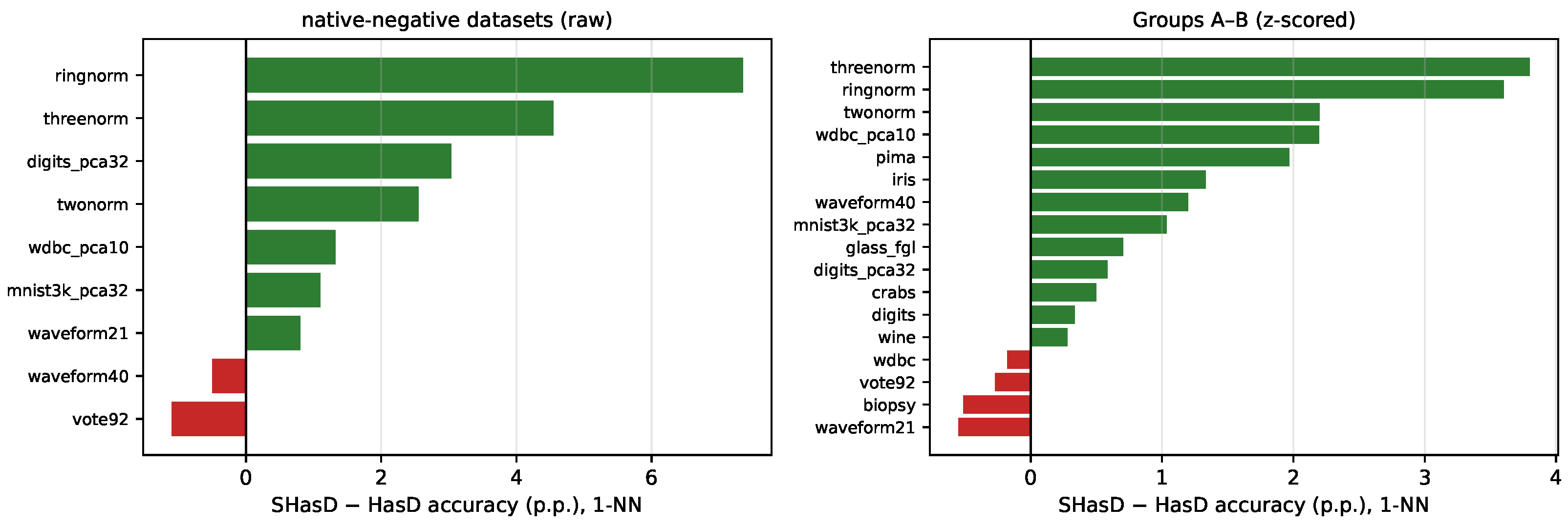
Table 3 reports 1-nearest-neighbor (1-NN) accuracy on the native-negative datasets (raw), and Table 4 on all 17 datasets after z-scoring. SHasD achieved the second-best mean rank among all ten measures on the z-scored suite after Bray–Curtis, and it improved significantly on HasD in both confirmatory comparisons: 7 wins/2 losses head-to-head on Group A raw (mean improvement + 2.1 percentage points, 95 % CI [ + 0.1 , + 4.1 ] , rank-biserial r = 0.78 ; exact Wilcoxon p = 0.039 , Holm-adjusted p = 0.040 ) and 13 wins/4 losses on the z-scored suite ( + 1.1 p.p. on average, 95 % CI [ + 0.4 , + 1.7 ] , r = 0.79 ; p = 0.0026 , Holm-adjusted p = 0.010 ). The largest improvements appear exactly where the sign structure matters: zero-centered Gaussian-mixture geometry (ringnorm + 7.4 p.p., threenorm + 4.6 p.p. raw) and PCA-projected real data (digits_pca32 + 3.0 p.p.). Figure 3 shows differences among the datasets. The monotone variant SHasD-R behaved similarly: it beat HasD on 8 of the 9 native-negative datasets ( + 2.0 p.p., 95 % CI [ 0.4 , + 4.3 ] , r = 0.96 ; p = 0.0078 , Holm-adjusted p = 0.023 ) and on 12 of the 17 z-scored datasets ( + 0.8 p.p., 95 % CI [ 0.1 , + 1.7 ] , r = 0.62 ; p = 0.0202 , Holm-adjusted p = 0.040 ), ranking just behind D s overall, consistent with its slightly more conservative treatment of sign-straddling pairs. All four confirmatory tests remained significant at α = 0.05 after Holm correction. Note that the two SHasD-R confidence intervals on the mean difference included zero: the dataset-level differences were heterogeneous (a few large gains alongside several small losses), and the rank-based statistics, which were less sensitive to the magnitude of single datasets, carried the inference here. Proposition 1 guaranteed that the distance matrices produced by the two measures on the Group B raw data would be identical to machine precision, and residual deviations were then only in sub-percent accuracy, due to the tie-breaking of neighbors in floating-point arithmetic.
  • Multi-measure rank analysis.
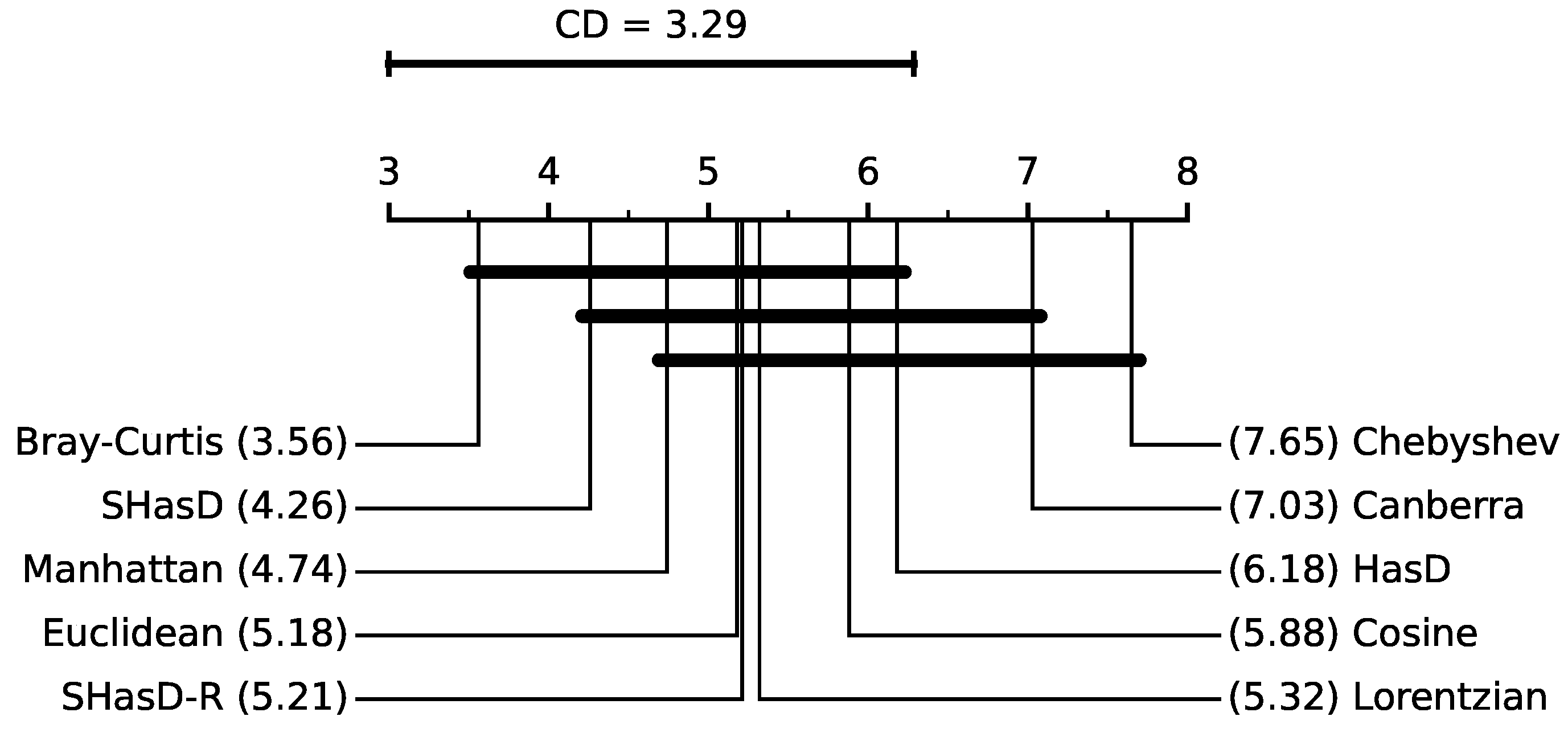
Figure 4 places the ten-measure comparison on the z-scored suite under the Demšar critical-difference lens [72]. The Friedman omnibus test rejected equality of the ten measures ( χ F 2 ( 9 ) = 25.6 , p 0.0024 ). The Nemenyi critical difference at α = 0.05 for ten measures on 17 datasets was CD = 3.29 : under this conservative all-pairs criterion only the largest separations were individually significant (Bray–Curtis and SHasD vs. Chebyshev; Bray–Curtis vs. Canberra). In particular, the  1.92 -rank gap between SHasD ( 4.26 ) and HasD ( 6.18 ) did not by itself exceed the critical difference. The evidence that SHasD improves on HasD therefore rests on the confirmatory paired Wilcoxon tests above—which were designed for precisely this one-to-one comparison and survived Holm correction—and not on the all-pairs rank analysis. Accordingly, we phrase all cross-measure statements in this paper descriptively (via mean ranks) and confine claims of statistical significance to the paired SHasD and SHasD-R vs. HasD comparisons on signed data.

7.2. Effect of k

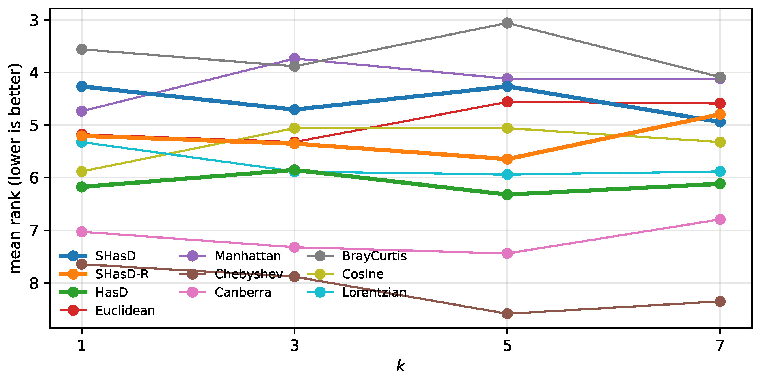
Figure 5 tracks the mean rank of each measure on the z-scored suite for k { 1 , 3 , 5 , 7 } . SHasD’s advantage over HasD is stable across k (rank gap between 0.8 and 1.8 ), indicating that the improvement is a property of the induced neighborhoods rather than of a particular k.

7.3. The Bounded [ 1 , 1 ] Regime

The comparison of groups A and B is presented in Table 5. Per-feature min–max scaling to [ 1 , 1 ] mimicked pipelines with bounded activations and normalized signal pathways. The difference between SHasD and HasD was effectively zero (10 wins, 7 losses, 0.0 p.p., p = 0.89 ; this comparison is exploratory). The sign-asymmetry distortion in (3) is proportional to feature magnitude and is numerically negligible for features in [ 1 , 1 ] . In this uniform-scale, outlier-free regime, the plain Manhattan and Euclidean metrics performed best, with BC’s adaptive-scale advantage reduced (mean rank 4.68 ) and Canberra’s performance deteriorating (mean rank 8.0 ) due to its sensitivity near the origin. This was not a failure of the method, but a scope statement: symmetrization matters only in unbounded signed contexts (e.g., z-scores, PCA, and embedding coordinates) and is neutral—never detrimental—on tightly bounded data.

7.4. Native Outliers: Group C

Table 6 reports the regime HasD was designed for—signed data whose outliers are real, not injected. Here SHasD attained the best mean rank of the ten measures ( 3.67 , vs. Lorentzian 3.75 , SHasD-R 4.17 , HasD 4.75 , Bray–Curtis 5.00 , Euclidean 6.83 ); with only six datasets the Nemenyi critical difference was 5.53 , so this ranking is descriptive (exploratory), and we do not claim statistical separation among the leading measures. BC’s clean-data advantage disappeared once heavy tails were native, and Euclidean paid the classical price (on twonorm_t it trailed SHasD by 6.6  p.p., having led on the clean twonorm). SHasD-R beat HasD on 4 of 6 datasets. We note for completeness that the two stock-volatility tasks carried weak class signal (51– 52 % , all measures within one point); the FX task and the contaminated generators carried the discrimination.

7.5. Robustness to Noise and Outliers

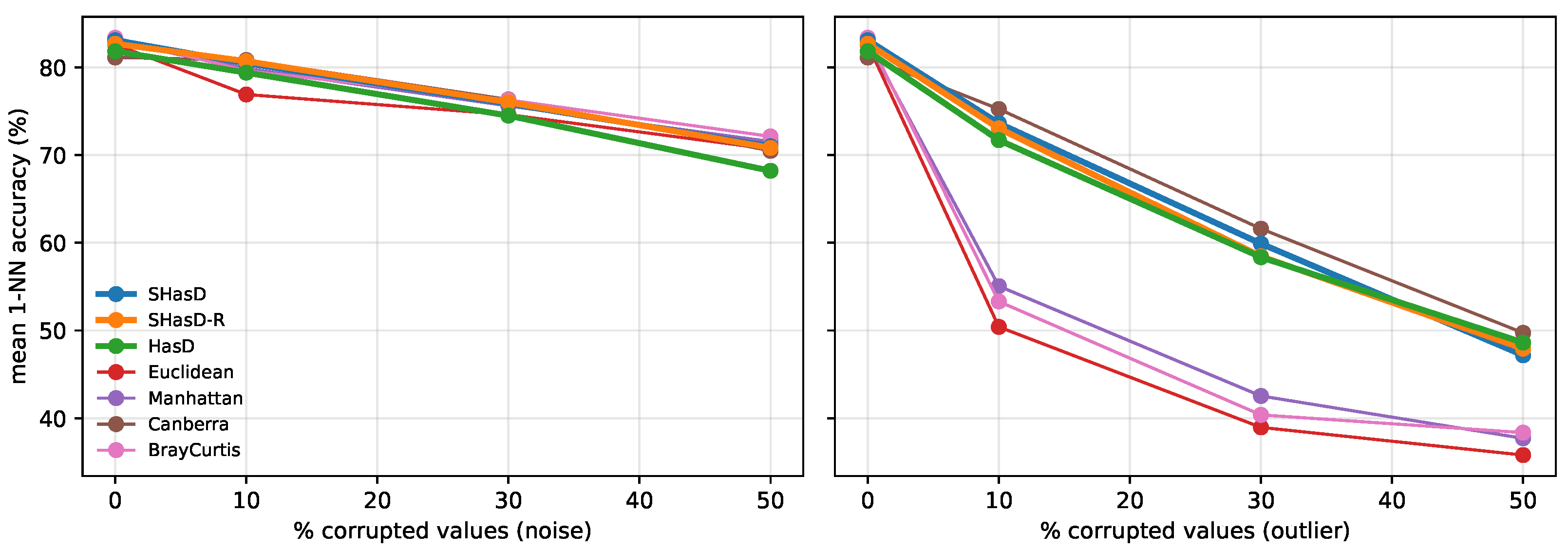
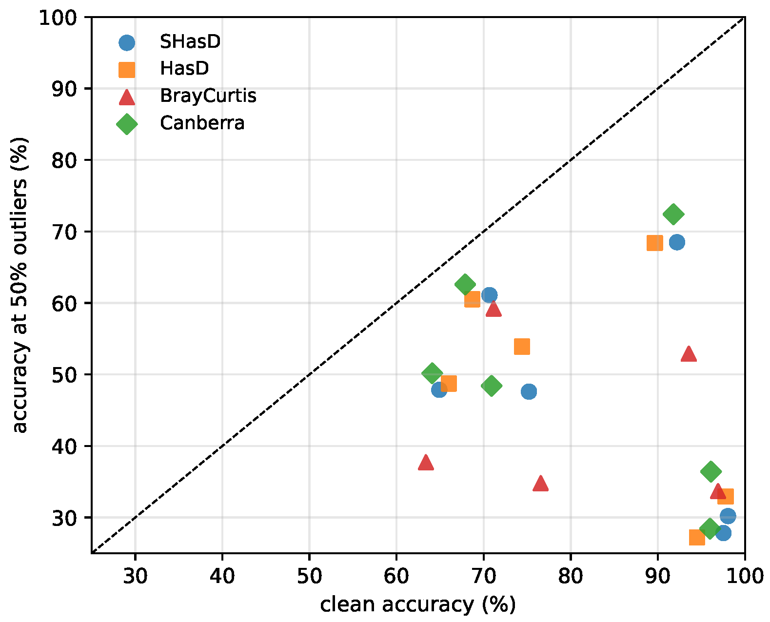
Table 7 and Figure 6 summarize accuracy under increasing corruption on six representative datasets. Under additive Gaussian noise the bounded measures degraded gracefully and SHasD remained ahead of HasD at every level. Under outlier substitution the picture is dramatic and confirms the HasD design philosophy: unbounded measures collapsed (Euclidean fell from 83% mean accuracy on clean data to 36% at 50 % corruption), while the per-dimension-bounded family (SHasD, HasD, Canberra) degraded far more slowly. SHasD preserved this hallmark robustness of HasD—it was among the top two measures at 10 % and 30 % outlier corruption—while additionally removing the sign asymmetry. Figure 7 condenses the trade-off: on clean data BC and SHasD were comparable, but under 50 % outlier substitution the BC points fell far below the SHasD points for every dataset.

7.6. Interpretability: Where and Why the Metrics Differ

Since all distances in the Hassanat family are a sum of per-dimension terms, each feature’s contribution to a given pairwise distance is given in closed form; the metric is self-explanatory, without the need for any post hoc approximation. We use this to explain the robust mechanism on three different levels:
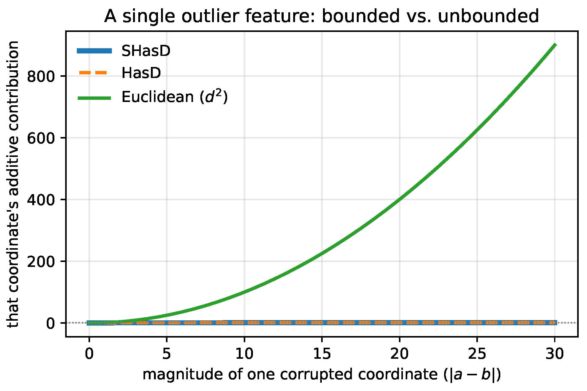
Mechanism (Figure 8). A single coordinate whose value is corrupted by | a b | contributes min ( · ) 1 under SHasD and HasD but grows without bound under Euclidean. One outlier feature can therefore dominate a Euclidean distance entirely, while it can shift a Hassanat distance by at most one unit.
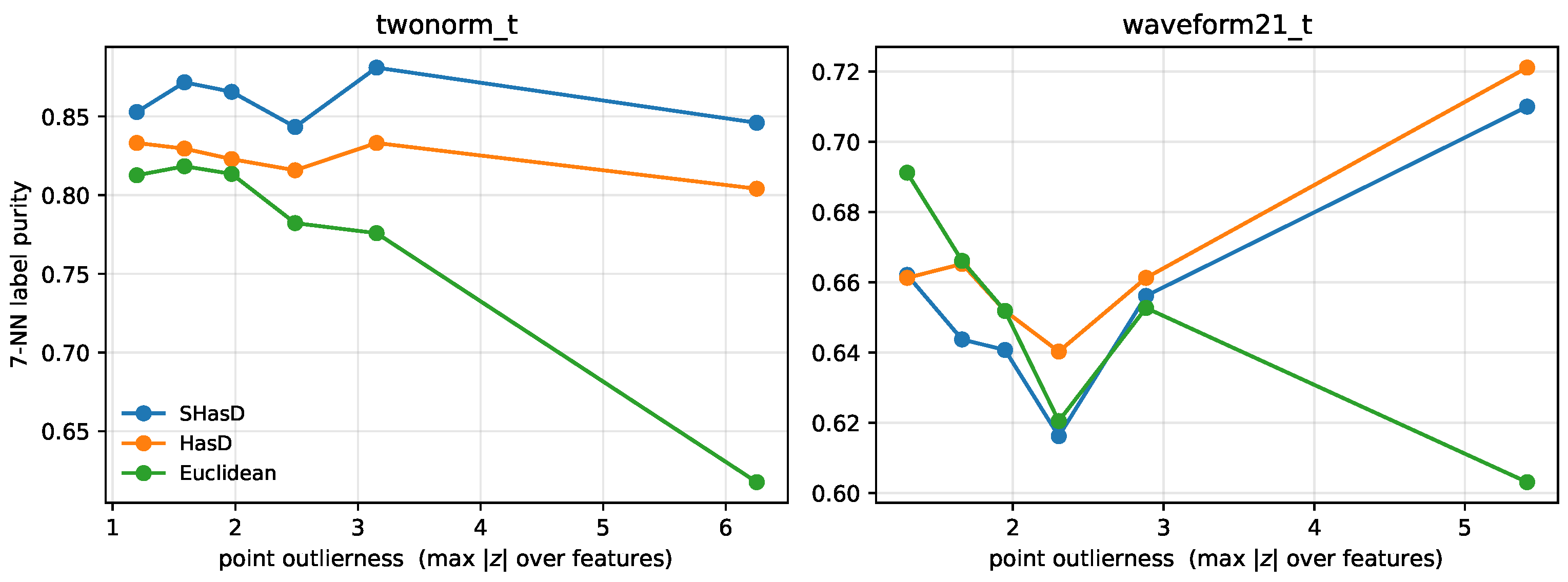
Population (Figure 9). Binning test points by outlierness (maximum | z | -score across features) and measuring the label purity of each point’s seven nearest neighbors, Euclidean purity falls steeply for the most extreme points (on twonorm_t, from  0.81 to 0.62 ) while SHasD stays essentially flat (≈0.85): the points SHasD “rescues” are precisely the high-magnitude ones.
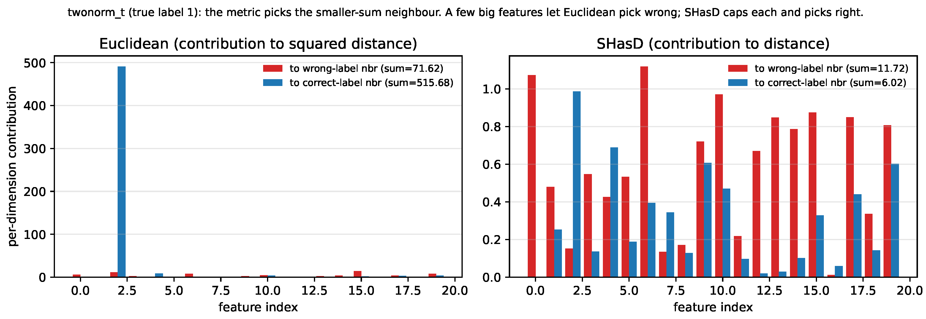
Instance (Figure 10). For a single test point that Euclidean misclassifies but SHasD classifies correctly, the per-dimension decomposition to the two candidate neighbors shows the cause directly: one heavy-tailed coordinate contributes ∼22 of Euclidean’s distance to the correct-label neighbor, pushing its total above the wrong-label neighbor; SHasD caps that same coordinate below 1, and the correct neighbor wins. The misclassification is explained by a single feature, and so is the fix.

7.7. Runtime

Because (4) is branch-free, SHasD is also cheaper to evaluate than (1): on a 1000 × 1000 × 32 pairwise-distance computation our vectorized implementation of SHasD ran about 2.9× faster than HasD ( 0.29 s vs. 0.84  s per million-pair block) ( numpy, single thread; see released code). Both measures are Θ ( m ) per pair; the gap is the constant-factor effect of branch elimination analyzed in Remark 4.

8. Discussion and Limitations

When does SHasD lose? On 2 of 9 native-negative and 4 of 17 z-scored datasets HasD was marginally better (at most 1.1 p.p.). These datasets (vote92, waveform variants, biopsy, wdbc) show no systematic pattern beyond small differences within fold noise; the Wilcoxon tests confirm the aggregate advantage is significant. Saturation and bounds. For sign-straddling pairs D s can exceed 1 and is not ray monotone in the saturated band (Section 5.3); applications that require the [ 0 , 1 ) bound or strict monotone-in-separation semantics should use SHasD-R, which provides both guarantees, remains significantly better than HasD, and trails D s by roughly one mean-rank point on the signed suites—only 0.2 0.4 percentage points of mean accuracy (Table 3, Table 4 and Table 6). Why not Bray–Curtis? BC attains the best mean rank on clean data in our suite, and it is worth explaining why this does not make it the answer. BC is the Manhattan distance normalized by the per-pair factor i | x i + y i | ; on zero-centered data this acts as a built-in adaptive scale with a cosine-like alignment effect, a good geometric fit to Gaussian and PCA-projected benchmarks (e.g., ringnorm, where class identity is carried largely by the vector norm). However, BC is not a metric, and on signed data this can be exhibited analytically rather than only empirically. Writing BC ( x , y ) = i | x i y i | / i | x i + y i | , take the one-dimensional triple x = 2 , y = 0 , z = 1 :
BC ( 2 , 0 ) = 2 2 = 1 , BC ( 0 , 1 ) = 1 1 = 1 ,
BC ( 2 , 1 ) = 3 1 = 3 > 2 = BC ( 2 , 0 ) + BC ( 0 , 1 ) ,
a violation of the triangle inequality by a factor of 3 2 ; and for sign-opposed vectors the denominator vanishes entirely ( BC ( t , t ) = 2 | t | / 0 is undefined). Consistent with this, in our analysis BC violated the triangle inequality on about 15 % of random signed triples; its [ 0 , 1 ] bound held only for non-negative numbers; and the vanishing denominator made it numerically unstable precisely on the signed data, which this paper targeted. It was also fragile under gross corruption, falling to 38.4 % mean accuracy at 50 % outliers versus 47– 49 % for the SHasD/HasD family (Table 7), because a single extreme value perturbed the global normalizer, whereas the HasD family capped each dimension’s contribution. BC is thus a strong clean-data heuristic, but not a substitute for a bounded, provable metric. Scope of experiments. Our suite mixed real data (12 datasets) with classic synthetic generators (5 Breiman benchmarks used precisely because their geometry is zero-centered); results on larger, high-dimensional embedding spaces (e.g., deep feature spaces, which are also sign-symmetric by construction) are a natural next step. Other learners and applicability beyond KNN. We isolate the distance with KNN, following standard practice; SHasD is directly applicable wherever HasD has been used (clustering, retrieval, oversampling validation, etc. [12]). Several such uses deserve comment. In clustering (k-medoids, DBSCAN, hierarchical linkage, graph-based partitioning [8]), SHasD can replace the dissimilarity directly, and its per-coordinate bound limits the leverage of outlying points on cluster shape; centroid-based methods such as k-means, however, require a mean that is optimal for the metric, which SHasD does not supply in closed form. In retrieval and nearest-neighbor search, the metric property matters concretely: triangle-inequality-based indexes (VP-trees, cover trees, metric trees) are sound for SHasD and SHasD-R but not for non-metric scores like Bray–Curtis, and the [ 0 , 1 ) per-dimension bound of SHasD-R gives calibrated, dimension-normalized thresholds. In metric learning, the sign-symmetric normalizer could serve as a fixed robust base metric on top of learned embeddings—which are zero-centered by construction, exactly the regime studied here. Limitations. Beyond the scope items above, three limitations are worth stating explicitly: (i) SHasD’s per-dimension sum ignores feature correlations (as do Manhattan, Canberra, and HasD); (ii) the saturated cross-sign band of D s (Section 5.3) trades ray monotonicity for adaptivity, and although SHasD-R repairs this, it trails D s by roughly one mean-rank point on the signed suites (a small fraction of a percentage point in mean accuracy, 0.2 0.4 p.p.); (iii) our evidence is confined to KNN classification on datasets of moderate size and dimension, and the behavior inside learned-embedding retrieval stacks and clustering objectives remains to be established empirically.

9. Conclusions

We showed that the negative branch of the Hassanat distance discards magnitude information and breaks reflection symmetry, and that the entire two-branch definition can be replaced by the single expression | a b | / ( 1 + max ( | a | , | b | ) ) ; a companion form, SHasD-R, normalizes by the range of { a , b , 0 } and additionally guarantees ray monotonicity and the [ 0 , 1 ) per-dimension bound. The reformulation is provably a metric, coincides exactly with HasD on non-negative data, restores sign symmetry, simplifies and accelerates computation, and in our experiments significantly outperformed HasD on data with negative values—which, through standardization and projection, covers much of the data seen in modern pipelines—while preserving HasD’s celebrated robustness to outliers. Under native heavy-tailed outliers—the regime the Hassanat family targets—SHasD attained the best mean rank of the ten measures compared, a descriptive result whose statistical confirmation on larger dataset collections we leave to future work. Beyond the empirical findings, the revised theoretical picture is that SHasD is topologically equivalent to the Euclidean metric, complete, and the unique backward-compatible member of a broader family of admissible sign-symmetric normalizations (Section 5.4 and Section 5.5).
  • Practical guidance.
Within the settings studied in this work—KNN classification on tabular data under the three normalization regimes considered—SHasD behaved as a reliable drop-in replacement for HasD: it is on par for non-negative data, outperformed HasD on signed data, and is more efficient; we therefore recommend it as the default choice in comparable settings, while noting that broader claims await evaluation on other tasks and learners. Use SHasD-R when the ray monotonicity or the [ 0 , 1 ) per-dimension constraint matters (metric indexing, calibrated thresholds). We study SHasD + ND for embedding-like, zero-centered data with class information in vector norm or orientation. We advise against Bray–Curtis when the data may contain outliers or metric assurances are needed.
  • Future directions.
Several extensions appear promising: weighted variants that assign per-feature weights inside the sign-symmetric normalizer; adaptive or parameterized members of the admissible family of Section 5.5 (e.g., ψ ( t ) = c t or ψ ( t ) = t α ), where the parameter is tuned to the data’s tail behavior; extensions of the sign-symmetric construction to generalized metric frameworks such as b-metrics, partial metrics, and fuzzy metric spaces (Section 2); a full characterization of pair-dependent admissible normalizers; and evaluation within clustering, retrieval, metric learning, and approximate nearest-neighbor indexing, where the completeness and boundedness properties established here are directly relevant.
  • Reproducibility.
All the datasets used in this paper are publicly available or generated by published generators with fixed seeds. The full experimental code (including data preparation, metrics, cross-validation, figures and tables) is provided with this paper and available from the corresponding author on reasonable request.

Author Contributions

Conceptualization, A.B.H. and A.S.T.; methodology, A.B.H., A.S.T., M.S.A. and G.N.A.; software, M.S.A. and G.N.A.; validation, A.B.H., A.S.T., M.S.A. and G.N.A.; formal analysis, A.B.H., A.S.T., M.S.A. and G.N.A.; investigation, A.B.H., A.S.T., M.S.A. and G.N.A.; resources, M.S.A. and G.N.A.; data curation, M.S.A. and G.N.A.; writing—original draft preparation, A.B.H., A.S.T., M.S.A. and G.N.A.; writing—review and editing, A.B.H., A.S.T., M.S.A. and G.N.A.; visualization, A.S.T.; supervision, A.B.H.; project administration, A.B.H. All authors have read and agreed to the published version of the manuscript.

Funding

This research received no external funding.

Data Availability Statement

All datasets are either publicly available or generated from published generators with fixed seeds. The code for all experiments is included with this paper and is available from the corresponding author upon reasonable request.

Acknowledgments

During the preparation of this manuscript, the authors used a generative AI assistant (Anthropic’s Claude, versions Sonnet 4 and Opus 4; Anthropic, San Francisco, CA, USA) to condense and copy-edit the Related Work section from author-supplied sources and a reference list compiled by the authors, to standardize the formatting of bibliography entries, and for minor language refinement, as well as to assist in verifying the computational reproducibility of the reported results by re-running the authors’ released code and cross-checking the resulting tables and figures. No AI tool was used to generate research data, design experiments, or produce original scientific claims. All AI-assisted outputs were reviewed, verified, and edited by the authors, who take full responsibility for the entire content of the manuscript.

Conflicts of Interest

The authors declare no conflicts of interest.

Appendix A. Implementation Validation

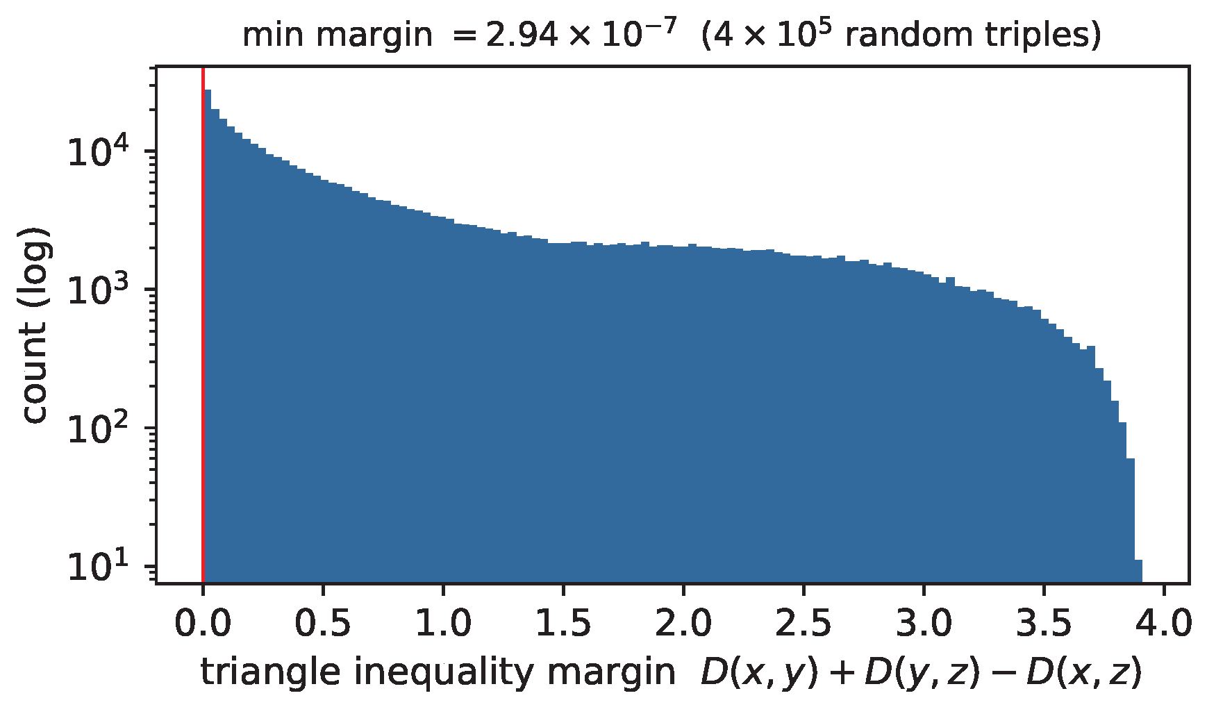
The metric property of D s and D r is established analytically by Theorems 1 and 2; the checks reported here are implementation diagnostics for the released code, not mathematical evidence. As a regression test of our vectorized implementation, we evaluated the triangle-inequality margin D s ( x , y ) + D s ( y , z ) D s ( x , z ) on 4 × 10 5 random triples drawn uniformly from [ 50 , 50 ] ; the margin was non-negative in every case (Figure A1), confirming that the implementation matches the analysis. The same harness is what detects the failures of the non-metric alternatives discussed in the main text (e.g., the vector-level normalization of Section 5.6 and Bray–Curtis, whose analytic counterexample is given in Section 8).
Figure A1. Empirical triangle-inequality margin of D s over 4 × 10 5 random triples in [ 50 , 50 ] , used as an implementation regression test. Consistent with Theorem 1, all margins are non-negative.
Symmetry 18 01225 g0a1

References

  1. Fix, E.; Hodges, J.L. Discriminatory Analysis, Nonparametric Discrimination: Consistency Properties; Technical Report; USAF School of Aviation Medicine: Dayton, OH, USA, 1951; p. 4. [Google Scholar]
  2. Cover, T.; Hart, P. Nearest neighbor pattern classification. IEEE Trans. Inf. Theory 1967, 13, 21–27. [Google Scholar] [CrossRef]
  3. Abu Alfeilat, H.A.; Hassanat, A.B.; Lasassmeh, O.; Tarawneh, A.S.; Alhasanat, M.B.; Eyal Salman, H.S.; Prasath, V.B.S. Effects of distance measure choice on k-nearest neighbor classifier performance: A review. Big Data 2019, 7, 221–248. [Google Scholar] [CrossRef] [PubMed]
  4. Cha, S.-H. Comprehensive survey on distance/similarity measures between probability density functions. Int. J. Math. Model. Methods Appl. Sci. 2007, 1, 300–307. [Google Scholar]
  5. Deza, M.M.; Deza, E. Encyclopedia of Distances; Springer: Berlin/Heidelberg, Germany, 2009. [Google Scholar]
  6. Li, J.; Li, J.; Wang, C.; Verbeek, F.J.; Schultz, T.; Liu, H. Outlier detection using iterative adaptive mini-minimum spanning tree generation with applications on medical data. Front. Physiol. 2023, 14, 1233341. [Google Scholar] [CrossRef] [PubMed]
  7. Dai, W.; Fan, R.; Nan, J. Simultaneous fault diagnosis for control valve using feature fusion and multilabel classification framework considering fault similarity. IEEE Trans. Instrum. Meas. 2025, 74, 3519211. [Google Scholar] [CrossRef]
  8. Geng, J.; Zhao, S.; Weizhe, W.; Li, Q. Adaptive graph partitioning for clustering datasets with heterogeneous density. ACM Trans. Knowl. Discov. Data 2025, 20, 2. [Google Scholar] [CrossRef]
  9. Zhang, H.; Jiang, L.; Yu, L. Attribute and instance weighted naive Bayes. Pattern Recognit. 2021, 111, 107674. [Google Scholar] [CrossRef]
  10. Moussaoui, A.; Radenović, S. Fuzzy metric spaces: A survey on fixed point results, contraction principles and simulation functions. Fixed Point Theory Algorithms Sci. Eng. 2025, 2025, 24. [Google Scholar] [CrossRef]
  11. Hassanat, A.B. Dimensionality invariant similarity measure. J. Am. Sci. 2014, 10, 221–226. [Google Scholar]
  12. Hassanat, A.; Alkafaween, E.; Tarawneh, A.S.; Elmougy, S. Applications review of Hassanat distance metric. In Proceedings of the 2022 International Conference on Emerging Trends in Computing and Engineering Applications (ETCEA22), Amman, Jordan; IEEE: Piscataway, NJ, USA, 2022; pp. 1–6. [Google Scholar]
  13. Tarawneh, A.S. HasLoss: A novel Hassanat distance-based loss function for binary classification. Front. Artif. Intell. 2026, 8, 1690830. [Google Scholar] [CrossRef] [PubMed]
  14. Hofer, E.; Mohrenschildt, M.V. Locally-Scaled Kernels and Confidence Voting. Mach. Learn. Knowl. Extr. 2024, 6, 1126–1144. [Google Scholar] [CrossRef]
  15. Jiřina, M.; Krayem, S. The Distance Function Optimization for the Near Neighbors-Based Classifiers. ACM Trans. Knowl. Discov. From Data 2022, 16, 101. [Google Scholar] [CrossRef] [PubMed]
  16. Uddin, S.; Haque, I.; Lu, H.; Moni, M.A.; Gide, E. Comparative performance analysis of K-nearest neighbour (KNN) algorithm and its different variants for disease prediction. Sci. Rep. 2022, 12, 6256. [Google Scholar] [CrossRef] [PubMed]
  17. Lin, K.Y.C. Optimizing variable selection and neighbourhood size in the K-nearest neighbour algorithm. Comput. Ind. Eng. 2024, 191, 110142. [Google Scholar] [CrossRef]
  18. Lin, K.Y.C. Optimizing hyperparameters in the k-NN classifier to maximize Fβ score. In Proceedings of the AIP Conference Proceedings; AIP Publishing LLC: Melville, NY, USA, 2025; p. 400027. [Google Scholar] [CrossRef]
  19. Hassanat, A.B.; Alkasasbeh, A.A.; Alkafaween, E.; Lasassmeh, O.; Almohammadi, K.; Alrashidi, M.; Alzahrani, A.; Alamri, M.; Tarawneh, A.S. On the Optimality of k = n in k-Nearest Neighbor Classification: Sub-Optimality Rates, Dimension-Aware Selection, and Hassanat Distance Comparison. Preprints 2026. [Google Scholar] [CrossRef]
  20. Guo, Z.; Liu, G.; Liu, W.; Ni, Z.; Jiang, F. GWKNN: An enhanced k-nearest neighbor algorithm with G metric reconstruction and Grey Wolf Optimizer. Sci. Rep. 2026, 16, 8857. [Google Scholar] [CrossRef] [PubMed]
  21. Hadi, D.; Kurniawan, I.; Mubais, A.; Sulistyawati, D.R. Feature selection and distance metric comparison of the k-nearest neighbor algorithm on large software effort estimation datasets. In Proceedings of the AIP Conference Proceedings; AIP Publishing LLC: Melville, NY, USA, 2026; p. 070067. [Google Scholar] [CrossRef]
  22. Hassanat, A.B.; Tarawneh, A.S.; Alhasanat, A.S.; Alghamdi, M.; Almohammadi, K.; Tarawneh, Z. ICT: Iterative clustering with training: Preliminary results. In Proceedings of the 2025 International Conference on New Trends in Computing Sciences (ICTCS); IEEE: Piscataway, NJ, USA, 2025; pp. 97–104. [Google Scholar] [CrossRef]
  23. Bidye, P.; Borkar, P.; Rakesh, N. High performance GPU implementation of KNN algorithm: A review. MethodsX 2025, 42, 103633. [Google Scholar] [CrossRef] [PubMed]
  24. Ehsani, R.; Drabløs, F. Robust distance measures for k-NN classification of cancer data. Cancer Inform. 2020, 19, 1176935120965542. [Google Scholar] [CrossRef] [PubMed]
  25. Na, J.; Wang, Z.; Lv, S.; Xu, Z. An extended k nearest neighbors-based classifier for epilepsy diagnosis. IEEE Access 2021, 9, 73910–73923. [Google Scholar] [CrossRef]
  26. Sujdha, C.; Selvi, R.T.; Bharathidason, S. Improving the Classification Performance for the Effective Diagnosis of Diseases Using Optimized Weighted KNN on Clinical Dataset. Indian J. Sci. Technol. 2025, 18, 215–222. [Google Scholar] [CrossRef]
  27. Al-Khlifeh, E.; Tarawneh, A.S.; Almohammadi, K.; Alrashidi, M.; Hassanat, R.; Hassanat, A.B. Decision tree-based learning and laboratory data mining: An efficient approach to amebiasis testing. Parasites Vectors 2025, 18, 33. [Google Scholar] [CrossRef] [PubMed]
  28. Yusran, M.; Sadik, K.; Soleh, A.M.; Suhaeni, C. Effect of Feature Normalization and Distance Metrics on K-Nearest Neighbors Performance for Diabetes Disease Classification. J. Math. Comput. Stat. 2025, 8, 341–354. [Google Scholar] [CrossRef]
  29. Febriani, S.M.N.N.; Setyoningrum, N.G.; Mulyani, E.D.S.; Putra, Y.P.; Fauzi, R.R. Sentiment analysis of public emotions on Twitter during COVID-19 pandemic using k-Nearest Neighbors algorithm. In Proceedings of the AIP Conference Proceedings; AIP Publishing LLC: Melville, NY, USA, 2025; p. 040011. [Google Scholar] [CrossRef]
  30. Nasiri, E.; Milanova, M.; Nasiri, A. Video Surveillance Framework Based on Real-Time Face Mask Detection and Recognition. In Proceedings of the 2021 International Conference on INnovations in Intelligent SysTems and Applications (INISTA); IEEE: Piscataway, NJ, USA, 2021; pp. 1–7. [Google Scholar] [CrossRef]
  31. Nasiri, E.; Milanova, M.; Nasiri, A. Masked face detection using artificial intelligent techniques. In New Approaches for Multidimensional Signal Processing: Proceedings of International Workshop, NAMSP 2021; Springer: Cham, Switzerland, 2022; pp. 3–34. [Google Scholar] [CrossRef]
  32. Anwar, M.; Hellwich, O. An Embedded Neural Network Approach for Reinforcing Deep Learning: Advancing Hand Gesture Recognition. J. Univers. Comput. Sci. 2024, 30, 957. [Google Scholar] [CrossRef]
  33. Zhu, J.; Ma, X.; Yu, D.; Li, Y.; Zhao, Y. Image quality difference perception ability: A BIQA model effectiveness metric based on model falsification method. Expert Syst. Appl. 2025, 260, 125349. [Google Scholar] [CrossRef]
  34. Wang, L.; Wu, H.; Yu, Y.; Yu, W.; Chen, S.; Wang, J. Gate-conv SVDD: An anomaly detection framework for fault inspection of photovoltaic panels using UAVs. IEEE Internet Things J. 2025, 12, 7890–7902. [Google Scholar] [CrossRef]
  35. Kancharla, C.R.; Vankeirsbilck, J.; Vanoost, D.; Boydens, J.; Hallez, H. Latent dimensions of auto-encoder as robust features for inter-conditional bearing fault diagnosis. Appl. Sci. 2022, 12, 965. [Google Scholar] [CrossRef]
  36. Bisht, K.S.; Ahamad, N.; Awasthi, S. Efficient Fault Classification in Distributed Generation Systems using M-KNN and Grid Search Techniques. Int. Energy J. 2025, 25, 45–56. [Google Scholar] [CrossRef]
  37. Bisht, K.S.; Ahamad, N.; Awasthi, S. A Comprehensive Analysis of Various KNN Algorithms for Fault Classification in a Smart Grid. J. Inst. Eng. Ser. B 2026, 107, 435–446. [Google Scholar] [CrossRef]
  38. Sarakum, T.; Sukpancharoen, S. Non-destructive sweetness classification of Khao Tang Kwa pomelos using machine learning with acoustic and image processing. J. Food Compos. Anal. 2025, 142, 107385. [Google Scholar] [CrossRef]
  39. Kozubal, J.V.; Kania, T.; Tarawneh, A.S.; Hassanat, A.; Lawal, R. Ultrasonic assessment of cement-stabilized soils: Deep learning experimental results. Measurement 2023, 223, 113793. [Google Scholar] [CrossRef]
  40. Hase, V.J.; Bhalerao, Y.J.; Verma, S.; Wakchaure, V.; Vikhe, G. Intelligent threshold prediction in hybrid mesh segmentation using machine learning classifiers. Int. J. Manag. Technol. Eng. 2018, 8, 1426–1442. [Google Scholar]
  41. Begovic, M.; Causevic, S.; Memic, B.; Haskovic, A. AI-aided traffic differentiated QoS routing and dynamic offloading in distributed fragmentation optimized SDN-IoT. Int. J. Eng. Res. Technol. 2020, 13, 1880–1895. [Google Scholar]
  42. Alkanhel, R.; Chaaf, A.; Samee, N.A.; Alohali, M.A.; Muthanna, M.S.A.; Poluektov, D.; Muthanna, A. DEDG: Cluster-based delay and energy-aware data gathering in 3D-UWSN with optimal movement of multi-AUV. Drones 2022, 6, 283. [Google Scholar] [CrossRef]
  43. Valenzuela, N.P.; Zabala-Blanco, D.; Guaña-Moya, J.; Játiva, P.P.; Cañizares, M.R.; Azurdia-Meza, C. Visible Light Positioning for 2D Indoor Environments via the Standard Extreme Learning Machine. In Proceedings of the 2025 IEEE Latin-American Conference on Communications (LATINCOM); IEEE: Piscataway, NJ, USA, 2025; pp. 219–224. [Google Scholar] [CrossRef]
  44. Shi, Q.; Bao, Y.; Shen, Q.; Shi, Z.; Gao, R. Dynamic and Multi-Graph Approaches for Connected Traffic Flow Prediction. In Connected Vehicles Traffic Prediction: Emerging GNN Methods; Springer: Cham, Switzerland, 2025; pp. 105–139. [Google Scholar] [CrossRef]
  45. Al-Nuaimi, D.H.; Isa, N.A.M.; Akbar, M.F.; Abidin, I.S.Z. AMC2-Pyramid: Intelligent pyramidal feature engineering and multi-distance decision making for automatic multi-carrier modulation classification. IEEE Access 2021, 9, 137560–137583. [Google Scholar] [CrossRef]
  46. Özarı, Ç.; Can, E.N.; Aliçi, A. Forecasting sustainable development level of selected Asian countries using M-EDAS and k-NN algorithm. Int. J. Soc. Sci. Educ. Res. 2023, 9, 101–112. [Google Scholar]
  47. Feng, L.; Sinchai, A. Time series forecasting using transfer learning with an attention-revamped transformer: A case study of financial instruments. Arab. J. Sci. Eng. 2025, 50, 19569–19595. [Google Scholar] [CrossRef]
  48. Torkzaban, M. Bankruptcy Prediction Models: A Comparative Analysis. Ph.D. Thesis, University of Padua, Padova, Italy, 2024. [Google Scholar]
  49. Pintong, K.P. Towards Lightweight Real-Time Identification, Classification, and Detection of Algorithm Behavior in Embedded Systems via the Power Side Channel. Ph.D. Thesis, State University of New York at Binghamton, Vestal, NY, USA, 2025. [Google Scholar]
  50. Veerachamy, R.; Ramar, R. Agricultural Irrigation Recommendation and Alert (AIRA) system using optimization and machine learning in Hadoop for sustainable agriculture. Environ. Sci. Pollut. Res. 2022, 29, 19955–19974. [Google Scholar] [CrossRef] [PubMed]
  51. Hazard, C.J.; Resnick, M.; Beel, J.; Xia, J.; Mack, C.; Glennie, D.; Fulp, M.; Maze, D.; Bassett, A.; Koistinen, M. A Theory of the Mechanics of Information: Generalization Through Measurement of Uncertainty (Learning is Measuring). arXiv 2025, arXiv:2510.22809. [Google Scholar] [CrossRef]
  52. Kartal, E.; Çalişkan, F.; Eskişehirli, B.B.; Özen, Z. P-adic distance and k-Nearest Neighbor classification. Neurocomputing 2024, 578, 127400. [Google Scholar] [CrossRef]
  53. Ondiek, J.O.; Ogada, K.; Mwalili, T. K-Nearest Neighbor Classification Accuracy Approach Using Weighted Distance Metrics and Three-Way. In Proceedings of Tenth International Congress on Information and Communication Technology: ICICT 2025; Springer Nature: Cham, Switzerland, 2025; Volume 4, p. 13. [Google Scholar]
  54. Czerwik, S. Contraction mappings in b-metric spaces. Acta Math. Et. Inform. Univ. Ostrav. 1993, 1, 5–11. [Google Scholar]
  55. Matthews, S.G. Partial metric topology. Ann. N. Y. Acad. Sci. 1994, 728, 183–197. [Google Scholar] [CrossRef]
  56. Amini-Harandi, A. Metric-like spaces, partial metric spaces and fixed points. Fixed Point Theory Appl. 2012, 2012, 204. [Google Scholar] [CrossRef]
  57. Kramosil, I.; Michálek, J. Fuzzy metrics and statistical metric spaces. Kybernetika 1975, 11, 336–344. [Google Scholar]
  58. George, A.; Veeramani, P. On some results in fuzzy metric spaces. Fuzzy Sets Syst. 1994, 64, 395–399. [Google Scholar] [CrossRef]
  59. Moussaoui, A.; Taş, N. New perturbed parametric metric spaces for distance modeling: Fixed-point analysis with applications to the fixed-circle problem. Fixed Point Theory Algorithms Sci. Eng. 2026, 2026, 15. [Google Scholar] [CrossRef]
  60. Corazza, P. Introduction to metric-preserving functions. Am. Math. Mon. 1999, 106, 309–323. [Google Scholar] [CrossRef][Green Version]
  61. Hassanat, A.B.; Alqaralleh, M.K.; Tarawneh, A.S.; Almohammadi, K.; Alamri, M.; Alzahrani, A.; Altarawneh, G.A.; Alhalaseh, R. A novel outlier-robust accuracy measure for machine learning regression using a non-convex distance metric. Mathematics 2024, 12, 3623. [Google Scholar] [CrossRef]
  62. Rockafellar, R.T. Convex Analysis; Princeton University Press: Princeton, NJ, USA, 1970. [Google Scholar]
  63. Pedregosa, F.; Varoquaux, G.; Gramfort, A.; Michel, V.; Thirion, B.; Grisel, O.; Blondel, M.; Prettenhofer, P.; Weiss, R.; Dubourg, V.; et al. Scikit-learn: Machine learning in Python. J. Mach. Learn. Res. 2011, 12, 2825–2830. [Google Scholar]
  64. Alvarez, R.M.; Nagler, J. Economics, issues and the Perot candidacy: Voter choice in the 1992 presidential election. Am. J. Political Sci. 1995, 39, 714–744. [Google Scholar] [CrossRef]
  65. LeCun, Y.; Bottou, L.; Bengio, Y.; Haffner, P. Gradient-based learning applied to document recognition. Proc. IEEE 1998, 86, 2278–2324. [Google Scholar] [CrossRef]
  66. Breiman, L. Bias, Variance, and Arcing Classifiers; Technical Report; Statistics Department, University of California: Berkeley, CA, USA, 1996; 460p. [Google Scholar]
  67. Breiman, L.; Friedman, J.; Olshen, R.; Stone, C. Classification and Regression Trees; Wadsworth: Belmont, CA, USA, 1984. [Google Scholar]
  68. Dua, D.; Graff, C. UCI Machine Learning Repository; University of California: Irvine, CA, USA, 2019. [Google Scholar]
  69. Venables, W.N.; Ripley, B.D. Modern Applied Statistics with S, 4th ed.; Springer: Berlin/Heidelberg, Germany, 2002. [Google Scholar]
  70. Huber, P.J. Robust estimation of a location parameter. Ann. Math. Stat. 1964, 35, 73–101. [Google Scholar] [CrossRef]
  71. Lance, G.N.; Williams, W.T. Computer programs for hierarchical polythetic classification (‘similarity analyses’). Comput. J. 1966, 9, 60–64. [Google Scholar] [CrossRef]
  72. Demšar, J. Statistical comparisons of classifiers over multiple data sets. J. Mach. Learn. Res. 2006, 7, 1–30. [Google Scholar]
Figure 1. Per-dimension distance to the fixed points 2 (solid) and 2 (dashed). (Left): HasD; the two profiles are not mirror images. (Middle): SHasD restores mirror symmetry, but its cross-sign tail decays after the peak at the mirror point. (Right): SHasD-R is mirror-symmetric and monotone along every ray. Note that each individual profile is intentionally asymmetric about its own anchor: the normalization by the larger magnitude makes the distance relative to scale (steeper toward zero, flatter away from it), the scale-adaptive behavior that defines the Hassanat family. Sign symmetry concerns the pair of profiles, not each profile alone; a profile symmetric about its anchor would imply translation invariance and forfeit boundedness.
Symmetry 18 01225 g001
Figure 2. Level sets (“balls”) of the two-dimensional distance to a center at ( 2 , 2 ) and at ( 2 , 2 ) . HasD balls (top) change shape when the center is reflected through the origin; SHasD balls (bottom) are reflections of one another. In each panel, the red “+” marks the center c; the colored curves are the level sets at r = 0.2 , 0.4 , , 1.2 , with inline labels and color both encoding the level r (darker = smaller r).
Symmetry 18 01225 g002
Figure 3. Head-to-head 1-NN accuracy difference, SHasD − HasD, in percentage points. (Left): native-negative datasets, raw. (Right): Groups A–B, z-scored. Green bars mark datasets on which SHasD improves on HasD (positive difference); red bars mark datasets on which HasD is better.
Symmetry 18 01225 g003
Figure 4. Critical-difference diagram (Nemenyi test, α = 0.05 ) for the ten measures on the 17 z-scored datasets. Lower mean rank is better; thick bars connect groups of measures whose mean ranks differ by less than CD = 3.29 and are therefore not separable by the conservative all-pairs test.
Symmetry 18 01225 g004
Figure 5. Mean rank (lower is better) over the 17 z-scored datasets as a function of k.
Symmetry 18 01225 g005
Figure 6. Mean 1-NN accuracy as the fraction of corrupted feature values grows, for additive Gaussian noise (left) and extreme-outlier substitution (right).
Symmetry 18 01225 g006
Figure 7. Clean accuracy vs. accuracy under 50 % outlier substitution, per dataset. The dashed line is no degradation; the bounded Hassanat family stays close to its clean performance while BC collapses.
Symmetry 18 01225 g007
Figure 8. Contribution of one corrupted coordinate to the distance, as its magnitude grows. SHasD and HasD saturate at 1; Euclidean is unbounded. The dotted horizontal line marks the per-coordinate saturation bound of 1; the SHasD and HasD curves coincide exactly on this configuration and are drawn with different line styles.
Symmetry 18 01225 g008
Figure 9. Seven-NN label purity vs. point outlierness. Euclidean degrades on the most outlying points; the bounded Hassanat measures do not.
Symmetry 18 01225 g009
Figure 10. Per-dimension decomposition of one flipped prediction (twonorm_t). Each metric selects the neighbor with the smaller total. A single high-magnitude feature dominates the Euclidean sums and selects the wrong-label neighbor; SHasD caps every feature and selects the correct one.
Symmetry 18 01225 g010
Table 1. Property summary: “=HasD” means equal distances on non-negative data. The only break of ray monotonicity for SHasD happens in the band where it is saturated with cross-signs ( D s > 1 ). The first five columns are structural (provable) properties; boundedness per coordinate is the structural ingredient behind outlier robustness. The last-but-one column, by contrast, is an empirical summary of the corruption experiments of Section 7 and should be read as observed, not guaranteed, behavior. A check mark (✓) indicates that the property holds; a cross (×) indicates that it does not.
MeasureMetricSign-SymmetricBounded/Coord.Ray-MonotoneRobust (Emp.)=HasD
HasD× [ 0 , 1 )
SHasD [ 0 , 2 ) partial
SHasD-R [ 0 , 1 )
SHasD + ND [ 0 , 2 ) moderate×
Bray–Curtis×unbounded×××
Canberra [ 0 , 1 ] ××
Euclideanunbounded××
Table 2. Datasets: “% Neg” is the percentage of negative feature values in the raw data.
DatasetSourcendClasses% Neg
digits_pca32UCI optdigits, PCA-32 (real)1797321049.8
mnist3k_pca32MNIST subset, PCA-32 (real)3000321050.1
ringnormBreiman 1996 generator [66]100020241.1
threenormBreiman 1996 generator [66]100020250.0
twonormBreiman 1996 generator [66]100020249.9
vote92R pscl::vote92 (real survey)9098313.3
waveform21Breiman et al. 1984 generator [67]100021319.8
waveform40Breiman et al. 1984 generator [67]100040333.8
wdbc_pca10UCI WDBC, z+PCA-10 (real)56910252.4
biopsyR MASS::biopsy = UCI BCW original (real)683920.0
crabsR MASS::crabs (real)200540.0
digitssklearn/UCI (real)179764100.0
glass_fglR MASS::fgl = UCI forensic glass (real)214966.4
irissklearn/UCI (real)150430.0
pimaR MASS::Pima = UCI Pima (real)532720.0
wdbcsklearn/UCI (real)5693020.0
winesklearn/UCI (real)1781330.0
bmw_volevir::bmw daily log-returns 1973–1996 (real)30005245.1
garch_fxEcdat::Garch FX log-returns 1980–1987 (real)18664250.3
siemens_volevir::siemens daily log-returns (real)30005244.6
threenorm_tthreenorm, t(2.5) noise (heavy-tailed synthetic)100020249.6
twonorm_ttwonorm, t(2.5) noise (heavy-tailed synthetic)100020250.0
waveform21_twaveform, t(2.5) noise (heavy-tailed synthetic)100021322.1
Table 3. 1-NN accuracy (%) on native-negative datasets (Group A, raw features). Best per row in bold.
DatasetSHasDSHasD-RHasDEuclid.Manh.Cheby.Canb.BrayC.CosineLorentz.
digits_pca3297.5296.9194.4998.8098.6497.9795.9998.7298.8097.69
mnist3k_pca3291.5791.0590.4793.2092.8891.3787.6793.2893.8091.85
ringnorm72.5574.9565.2068.0067.6565.2582.3086.8570.6566.70
threenorm74.8072.1070.2575.8075.2072.7071.7078.0078.2571.85
twonorm92.2091.1589.6593.7093.2092.0591.8093.5594.6092.10
vote9264.9165.7366.0164.4163.8763.2664.0863.3764.2464.85
waveform2175.2074.9074.4075.9076.1075.3070.9076.5573.7074.95
waveform4070.6571.5571.1578.0076.6074.2066.3574.8572.8074.05
wdbc_pca1093.7693.3292.4496.1396.9294.0388.2396.7595.8794.11
Mean81.4681.3079.3482.6682.3480.6879.8984.6682.5280.91
Mean rank5.676.568.333.004.006.448.332.893.895.89
Table 4. 1-NN accuracy (%) on all 17 datasets with z-score standardization (fitted per training fold). Best per row in bold.
DatasetSHasDSHasD-RHasDEuclid.Manh.Cheby.Canb.BrayC.CosineLorentz.
biopsy96.1996.7896.7195.4796.5694.9596.4196.8696.1296.56
crabs86.7586.7586.2589.2586.7588.7582.2586.0094.2586.75
digits97.8997.5297.5597.1497.9494.4496.2297.7897.2597.86
digits_pca3297.7297.3997.1497.4197.7592.5295.9998.1497.7297.66
glass_fgl75.7074.7575.0071.5274.0866.6276.1476.4271.6875.23
iris93.6793.6792.3394.6792.6795.3393.3393.3385.6792.33
mnist3k_pca3290.8590.4389.8291.8891.4886.2287.7092.4092.9290.32
pima70.6769.3668.7067.6668.1368.5867.8671.1470.1968.04
ringnorm70.1073.2066.5068.3567.5065.7082.5586.0063.4567.40
threenorm74.8572.8071.0575.7575.6072.7571.0577.0577.1572.20
twonorm91.8091.3089.6093.8593.2092.1592.2093.6094.6592.20
vote9264.5864.1964.8564.8064.1464.6964.3065.2964.6364.42
waveform2173.3573.4573.9074.9075.3071.9569.9572.3571.4074.60
waveform4073.0072.4571.8072.6574.1562.5071.1570.7567.2073.75
wdbc95.8795.6096.0595.2595.5294.1196.2295.3495.2695.96
wdbc_pca1091.9190.6889.7291.3990.3490.5188.0592.2790.1690.16
wine98.0698.0697.7895.2397.7692.6696.0996.9194.6698.59
Mean84.8884.6183.8184.5484.6482.0383.9785.9883.7984.35
Mean rank4.265.216.185.184.747.657.033.565.885.32
Table 5. 1-NN accuracy (%) under min–max [ 1 , 1 ] scaling (Groups A–B). Best per row in bold.
DatasetSHasDSHasD-RHasDEuclid.Manh.Cheby.Canb.BrayC.CosineLorentz.
biopsy96.3496.2096.5695.7696.7195.2596.2796.3495.9196.49
crabs87.2587.2586.2590.0086.7588.2583.2587.0091.0086.75
digits98.3398.2298.0898.8098.5897.9796.3898.5598.7898.39
digits_pca3298.1198.0598.0098.0898.3395.0295.7497.9798.0898.00
glass_fgl73.8673.6475.2570.1274.0667.1069.6173.5870.3574.53
iris94.0094.0093.6796.0094.0096.3393.3394.0090.0094.00
mnist3k_pca3291.5891.4391.3392.5391.9388.6788.0592.8292.7391.55
pima70.3869.9169.0768.7868.2371.2272.5571.0467.4768.79
ringnorm68.9070.0567.7568.4567.9065.7580.4087.0573.4067.75
threenorm73.8073.7572.4075.8574.9071.6570.2076.7077.1073.05
twonorm92.6592.5592.3593.5592.9592.0592.1093.2594.6092.20
vote9263.2663.9865.3564.2064.0861.7763.3763.8164.0966.01
waveform2174.2574.5574.7074.9575.3573.4569.6072.8071.1074.95
waveform4072.4073.1573.1074.2574.1065.6066.4569.9569.0573.60
wdbc95.3495.1795.3495.2695.1793.9495.0895.3494.2994.90
wdbc_pca1092.9793.2393.1493.7693.9493.4180.6793.0593.2393.94
wine96.6596.9398.0695.2597.2192.9695.7796.9395.5298.04
Mean84.7184.8384.7385.0384.9582.9682.8785.8984.5184.88
Mean rank5.155.445.504.093.887.888.004.685.444.94
Table 6. The 1-NN accuracy (%) on Group C: signed data with native heavy-tailed outliers (raw features). Best per row in bold.
DatasetSHasDSHasD-RHasDEuclid.Manh.Cheby.Canb.BrayC.CosineLorentz.
bmw_vol50.5550.5550.7350.5250.5851.0852.3550.6048.8050.68
garch_fx84.9784.9784.9784.3585.0283.7484.2284.6284.3085.02
siemens_vol52.1052.1052.0852.1752.0852.0851.8351.7249.3252.07
threenorm_t69.4068.1066.3064.1566.9059.5070.4070.3562.4568.65
twonorm_t87.1085.7083.9080.5083.1070.5086.3586.7577.2584.30
waveform21_t68.2568.6568.3563.7067.7058.1065.5566.2063.1069.15
Mean68.7368.3467.7265.9067.5662.5068.4568.3764.2068.31
Mean rank3.674.174.756.834.927.924.835.009.173.75
Table 7. Mean 1-NN accuracy (%) over six datasets under feature corruption. Best per row in bold.
ModeLevelSHasDSHasD-RHasDEuclid.Manh.Cheby.Canb.BrayC.CosineLorentz.
noise10%80.4680.7079.3976.9079.8774.0580.8379.5876.4080.60
noise30%75.8676.0274.5074.6175.6069.9476.3376.2874.3275.68
noise50%70.9970.8168.2070.6671.5367.4470.4872.1272.3071.47
outlier10%73.6273.0471.7150.4155.0546.5775.2553.3149.4870.69
outlier30%59.9058.4558.3538.9642.5437.8761.6040.3837.7952.24
outlier50%47.1847.9348.6235.8037.7134.7049.7338.3637.8443.65
Disclaimer/Publisher’s Note: The statements, opinions and data contained in all publications are solely those of the individual author(s) and contributor(s) and not of MDPI and/or the editor(s). MDPI and/or the editor(s) disclaim responsibility for any injury to people or property resulting from any ideas, methods, instructions or products referred to in the content.