Symmetric Complementarity of Co-Located Rail Systems on Urban Carbon Productivity

Abstract

Environmental protection has become a key priority for the Chinese government. This study examined the symmetric complementarity of spatial layouts between inter-city high-speed rail and urban subway systems. Their co-location formed a structurally symmetric low-carbon travel chain that bridged long-distance and short-distance trips. The study evaluated their joint effect on urban carbon productivity within a difference-in-differences framework. The baseline two-way fixed-effects DID estimate showed that the simultaneous operation of HSR and subway systems significantly improved urban carbon productivity, with an average increase of approximately 10.51% in treated cities relative to non-treated ones. This core finding remained qualitatively robust across a series of tests, including conditional coarsened exact matching (CEM), placebo simulations, sample exclusions, and decomposition of joint effects relative to individual rail impacts. Complementary nonparametric causal forest estimates yielded smaller but still significant effect sizes, providing supportive evidence for causal validity under weaker functional form assumptions. Heterogeneity analysis based on dynamic GDP grouping revealed that high-GDP cities experienced stronger emission reductions, while low-GDP cities benefited more from the economic growth dimension of carbon productivity. Empirical patterns aligned with the theoretical prediction of the transportation substitution mechanism. The positive effect of dual rail availability on carbon productivity was stronger in cities with higher private car stock, as shown by double machine learning interaction models. This finding only provided indirect evidence and did not constitute direct proof of actual modal shift behavior. The results exhibited magnitude asymmetry between parametric and nonparametric methods, yet all estimates consistently pointed to a positive qualitative direction. This consistency revealed directional symmetry in the causal conclusion. The study contributed by (1) examining the combined carbon productivity effect of co-located HSR and subway systems, (2) identifying the moderating role of private car stock in the transportation substitution mechanism, (3) revealing development-stage-based heterogeneity, (4) and combining machine learning methods with parametric causal inference as complementary robustness evidence. Policy implications suggested that high-GDP cities should prioritize expanding dual rail coverage and optimizing connections to amplify emission reductions, while low-GDP cities should focus on improving HSR connectivity with existing public transit systems and fostering low-carbon industrial development in line with local conditions.

1. Introduction

Global warming has become a major challenge for sustainable human development, and reducing greenhouse gas emissions, especially carbon dioxide emissions, has reached international consensus [1]. China has committed to peaking carbon emissions by 2030 and achieving carbon neutrality by 2060, and the task of reducing emissions is arduous [2]. As the world’s largest energy consumer and carbon emitter, China’s emission reduction actions are crucial to global climate governance, and improving the carbon productivity of cities that are the core carriers of carbon emissions is a key factor in achieving this goal [3]. By the end of 2023, China operated 159,000 km of railways including 45,000 km of high-speed rail. Around 80 percent of its “Eight Vertical and Eight Horizontal” high-speed rail corridors had entered service by October 2024. The country ran 256 metro lines stretching 9042.3 km and seven light rail lines with a length of 267.5 km in 2023 [4,5]. High-speed rail focuses on cross-regional long-distance transportation, while subway systems focuses on short-distance intra-city commuting. The two modes complement each other in spatial coverage and functional positioning. HSR and subway systems exhibit notable structural symmetry in spatial functions. The former serves cross-regional long-distance connections, while the latter focuses on intra-city short-distance commuting. This symmetric layout provides a physical basis for constructing a full-chain green transport system. Notably, this symmetry is confined to infrastructure co-location and does not imply station-level operational integration or seamless transfers.

Existing studies focus on the relationship between transportation infrastructure and carbon emissions, but there are obvious gaps. Firstly, the research perspective of existing studies focuses on a single mode of transportation, such as the inhibitory effect of high-speed rail (HSR) on carbon emissions of cities or enterprises [6], and the effects of subway systems on local pollutants such as PM2.5, ignoring the combined effects of inter-city HSR and urban subway systems; the environmental benefits of transport networks often stem from functional complementarity across multimodal infrastructure [7,8]. In addition, most existing studies examined changes in total carbon emissions separately [9], or only focused on economic growth effects [10], failing to integrate the dual dimensions for comprehensive evaluation. Third, heterogeneity analysis mostly revolved around urban scale and regional location [11], which lacked deeper discussion about the differences in economic development levels, making it difficult to explain the differences in policy effects in cities at different stages of development, and it cannot provide a basis for differentiated policy formulation. To directly address these three gaps, this study formulated the following core research questions: (1) Did the simultaneous operation of HSR and subway systems generate a combined effect on urban carbon productivity that differs from the simple sum of their individual impacts? (2) How did this joint effect operate through the dual channels of emission reduction and economic growth, and could it be decomposed to reveal the relative contributions of each channel? (3) Did the policy effect vary systematically across cities with different levels of economic development, and what role did the existing private car stock play in moderating the transportation substitution mechanism? To answer these questions, this paper incorporated both emission and growth dimensions into a unified carbon productivity framework, and adopted a dynamic GDP-based grouping strategy to capture development-stage heterogeneity, thereby providing a more nuanced empirical basis for differentiated transport policy design.

Based on this, the paper used a multi-period difference-in-differences (DID) model to identify the net effect. The marginal contributions of this paper include (1) evaluating the carbon productivity effect of having both HSR and subway systems available in the same city, addressing the limitation of single-mode transport studies, and enriching research on the environmental effects of multiple transport modes; (2) examining the dual effects of collaborative opening on both carbon emission reduction and economic growth, and exploring indirect evidence for a potential transportation substitution channel; (3) dividing the heterogeneous samples based on the level of economic development, and deeply analyzing the effect differences of cities at different development stages, so as to provide empirical support for the formulation of differentiated transportation policies; and (4) introducing machine learning methods, specifically causal forest for nonparametric causal inference and double machine learning (DML) for estimating interaction effects, to complement the parametric DID model. Unlike conventional robustness checks that rely on linear functional form assumptions, these machine learning approaches flexibly capture nonlinear confounder relationships, mitigate model misspecification bias through cross-fitting, and provide data-driven evidence on heterogeneous treatment effects and the moderating role of private car stock. This integration not only strengthens the credibility of the causal estimates, but also enables a more rigorous assessment of effect heterogeneity across cities, thereby enhancing both the robustness and the explanatory depth of empirical conclusions.

2. Literature Review

2.1. Research on the Influencing Factors of Carbon Productivity

As a core indicator to measure the coordination between economic development and carbon emissions, carbon productivity has been widely discussed, and existing research has been carried out from multiple dimensions such as policy, economy, technology, and infrastructure. At the policy level, the carbon trading pilot policy incentivizes enterprises to reduce emissions through the price mechanism [12,13], environmental regulation promotes green transformation through the dual effects [14], and green credit policies guide enterprises to invest in low-carbon projects through capital allocation [15]. At the economic level, the digital economy reduces carbon emission intensity through technological innovation and resource allocation optimization [16,17].

At the technical level, green technology innovation is the core driving force for carbon productivity improvement, and technology spillovers could further expand the scope of emission reductions for green innovation [18]. However, existing research mostly focuses on a single facility type, and there is a lack of research on the combined effects of multimodal transportation, which does not fully reflect the environmental benefits of transportation networks.

2.2. The Impact of High-Speed Rail on Carbon Emissions and Carbon Productivity

As a representative of green transportation, the environmental effects of HSR have received a lot of empirical support. From the perspective of macro cities, based on the panel data of 275 Chinese cities from 2003 to 2014, using the spatial difference-in-differences model, it was found that the improvement of high-speed rail service intensity significantly reduces urban CO₂ emissions through four mechanisms: transportation substitution, market integration, industrial structure upgrading, and technological innovation; moreover, the attenuation boundary of the spatial spillover effect was 1000 km [3]. Chen et al. (2023) pointed out that the opening of high-speed rail narrows the economic gap at the county level and indirectly optimizes the regional carbon emission pattern [19].

From the perspective of micro-enterprises, Chu and Chen used the multi-period DID model to confirm that the opening of HSR promoted green innovation. They used a multi-period DID model on a sample of listed industrial enterprises in China from 2007 to 2019; the results showed a decrease in financial constraints and a significant reduction in corporate carbon emissions. This effect was more significant in non-state-owned enterprises, heavy polluting enterprises, in cities with strict environmental regulations, and the central region [2].

However, the existing research is controversial. Some scholars believe that the consumption of building materials and energy input in the early stage of HSR construction may increase short-term emissions [20], and the agglomeration effect may lead to the expansion of transportation demand and offset some of the emission reduction effects. In addition, most studies focus on total carbon emissions and ignore the integrated consideration of economic growth [10]; therefore, the studies do not fully reflect the changes in carbon productivity or fully reveal the dual mechanisms of high-speed rail affecting carbon productivity.

2.3. The Impact of Subway Systems on Carbon Emissions and Carbon Productivity

In terms of carbon emissions, the emission reduction effect of subway systems mainly depends on the replacement of high-emission modes of transportation. Since subway systems are powered by electricity, the CO₂ emissions per passenger kilometer are only about 1/10 of that of private cars [21], and the expansion of subway network coverage can significantly reduce the carbon emission intensity of urban commuting [22,23]. Based on Seoul data, a well-developed subway network can significantly reduce commuting carbon emissions, and the emission reduction effect on suburban residents is stronger than that of urban residents [24].

However, there are two limitations of the existing research. First, it focuses more on the impact of a single metro network and does not consider coordination with cross-regional transportation, and the connection efficiency between cross-regional and urban transportation directly affects the overall emission reduction effect. Second, it focuses more on short-term emission changes, lacks long-term carbon productivity improvement mechanisms, and fails to integrate economic growth dimensions for comprehensive evaluation [22,25].

2.4. Research on Combined and Complementary Effects of Multimodal Transportation Infrastructure

The core of complementary effects is that different entities maximize the overall benefits through complementary functions, and the research on transportation infrastructure complementary effects mainly focuses on regional transportation integration, multi-mode transportation connection, and resource allocation optimization. In terms of regional transportation integration, taking the Shanghai–Nanjing high-speed railway as an example, it was found that high-speed rail can weaken urban administrative boundaries and promote regional market integration [8]. It was pointed out that the high-speed rail network in the Yangtze River Delta region can promote the agglomeration of productive service industries and optimize the regional industrial division of labor in terms of multi-mode transportation connection [26]. Chester and Horvath evaluated the effect of substituting highway and aviation with high-speed rail in the California corridor, and confirmed that it reduces greenhouse gas emissions during the life cycle through transportation substitution [27].

From a systematic policy design perspective, the Avoid–Shift–Improve (ASI) framework has been widely adopted as a mainstream analytical paradigm for structuring global transport decarbonization strategies. This coherent framework classifies low-carbon transport policies into three mutually reinforcing pathways. Avoid, which reduces unnecessary travel demand and shortens trip distances through integrated land use planning and travel demand management. Second, Shift, which redirects travel flows from high-emission private vehicles toward low-carbon public transport modes. Finally, Improve, which cut transport emission intensity via vehicle technology upgrades and clean energy substitution.

Against the backdrop of China’s rapid urbanization, accelerating private motorization, and the national strategic goal of achieving carbon neutrality by 2060, this framework gained particular policy relevance for guiding urban low-carbon transport transition using a provincial-level integrated assessment model covering 31 provinces in China. For instance, some researchers systematically evaluated 12 representative policy instruments under the ASI matrix, demonstrating that technology-focused Improve strategies yield the strongest carbon and air pollutant reduction effects, while Avoid and Shift strategies serve as indispensable complementary measures. Their study also documented pronounced regional disparities in policy effectiveness, highlighting the necessity of context-specific policy design [28].

City-level empirical evidence further corroborated the framework’s practical validity. Some researchers leveraged China’s Transit Metropolis Pilot program as a quasi-natural experiment and confirmed that comprehensive public transport policies achieve significant carbon abatement through all three ASI channels, with the Shift and Improve mechanisms contributing most prominently [29].

In the context of this study, the ASI framework, particularly its Shift component, offers a theoretically grounded lens for interpreting how the coordinated operation of high-speed rail (inter-city) and metro (intra-city) systems can substitute for private car use, thereby reducing transport-related carbon emissions and ultimately enhancing urban carbon productivity. Unlike previous studies that focused on either inter-city or intra-city transport in isolation, this study examined their combined impact, contributing to a more complete understanding of multi-level rail transit’s role in urban decarbonization.

Building upon the reviewed literature, several analytical issues motivated the present study. First, existing quantitative assessments typically treated inter-city high-speed rail and intra-city subway expansions as separate interventions. This separated approach left the networked effect from their co-location unquantified. Second, most empirical inquiries focused narrowly on aggregate emission volumes or local pollutant concentrations. Although carbon productivity as a dual-dimension indicator received conceptual attention in policy-oriented discussions, systematic econometric evaluation on multimodal rail integration and this metric remained absent. Third, while the ASI literature mentioned regional disparities in policy efficacy, what drives such heterogeneity, especially how city economic development stages moderate the shift from private cars to public transit, was not empirically tested. To address these issues, the present study evaluated the joint impact of opening HSR and subway systems on urban carbon productivity, with particular attention to the moderating pathways and stage-dependent characteristics, and investigated its heterogeneity mechanism.

3. Theoretical Analysis and Research Hypotheses

3.1. Coordinate the Opening of Mechanisms to Improve Urban Carbon Productivity

The complementary operation of high-speed rail and subway systems forms a multi-level green transport network. It reduces carbon emissions by replacing high-emission travel modes, and supports economic growth by improving travel efficiency, thereby enhancing urban carbon productivity. From a cross-regional perspective, HSR replaces some air and road passenger transport in medium- and long-distance travel with its advantages of high speed, low energy consumption, and low emissions. Per-passenger CO₂ emissions of aviation and highways are significantly higher than those of HSR. Åkerman confirmed that the life cycle greenhouse gas emissions of high-speed rail networks are significantly lower than those of road and aviation, and the emission reduction potential brought by the substitution effect is huge [30]. The life cycle assessment also showed that the replacement of high-speed rail by road and air can effectively reduce regional greenhouse gas emissions.

A study in the UK also confirmed that a well-developed subway network can significantly reduce the use of private cars and reduce commuting carbon emissions [23]. The combined coverage of the two systems formed a connected travel chain between inter-city and urban trips, reduced reliance on private cars during transfers, further expanded green transport coverage, lowered overall carbon intensity, improved travel efficiency and economic activity, and ultimately raised carbon productivity. The core value of dual rail systems lies in the complementarity of transport networks, which optimize resource allocation by improving spatial accessibility, thereby promoting green innovation and industrial upgrading and boosting carbon productivity. The joint operation of the two rail systems forms a spatially symmetric structure in substituting high-emission travel modes. HSR replaces aviation and inter-city road passenger transport, while subway systems displace private car usage within cities. This symmetric substitution reduces carbon emissions at both regional and urban scales, theoretically supporting the positive effect of co-location on carbon productivity.

Subway systems optimize the internal spatial structure of a city, shorten city commuting time, and improve the efficiency of the allocation of elements within a city [31]. The complementary operation of the two systems enables enterprises to more conveniently obtain cross-regional technology and human resources while reducing production and transaction costs in cities and promoting green technology innovation and industrial upgrading. By reducing carbon emissions, industrial upgrading can promote the decoupling of economic growth from carbon emissions [32] and ultimately achieve carbon productivity improvement.

Collaborative opening promotes the transformation of industrial structures to low-carbon systems by changing factor flow costs, thereby improving carbon productivity. On the one hand, the joint availability of high-speed rail and subway systems helps a city to attract knowledge-intensive and technology-intensive industrial agglomeration; the carbon emission intensity of such industries is significantly lower than that of traditional manufacturing.

On the other hand, the improvement of transportation networks reduces the living space of highly polluting enterprises, forcing them to carry out technological transformation or industrial transfer. At the same time, the commuting efficiency brought about by the collaborative opening promotes the joint availability of productive services and manufacturing, further optimizes the industrial structure, and achieves the decoupling of economic growth and carbon emissions [33].

Based on the above analysis, the joint opening of HSR and subway systems can reduce carbon emissions and promote economic growth through three mechanisms—transportation substitution, network coordination, and industrial structure upgrading—thereby improving urban carbon productivity. Among them, the traffic substitution effect is the most direct and observable transmission path for collaborative opening, so this paper empirically tested it as the core mechanism. The effect of network complementarity and industrial structure upgrading is more reflected in long-term and indirect structural effects, and its verification needs to rely on more microscopic data, which will be explained at the theoretical level and further deepened in future research. Based on this, the following hypotheses are proposed:

H1. 

The joint opening of high-speed rail and subway systems significantly improves urban carbon productivity.

3.2. The Heterogeneous Impact of Economic Development Level

The difference in the level of urban economic development led to different utilization efficiencies and mechanisms of transportation infrastructure, which in turn affected the carbon productivity effect of collaborative opening. On the one hand, high-GDP cities have a high number of private cars, strong commuting demand, and more space for subway substitution for private cars, resulting in more significant emission reduction effects. On the other hand, high-GDP cities have strong green innovation capabilities, sufficient R&D investment, and can amplify the carbon productivity improvement effect of collaborative opening through technological progress [34].

In low-GDP cities, the weak economic foundation may restrict the combined effect. First, the transportation network is not perfect in low-GDP cities, and the construction of transfer hubs lags behind, resulting in low connection efficiency between high-speed rail and subway systems, making it difficult to form effective complementary effects. Second, low-GDP cities are dominated by traditional manufacturing, with a low degree of low-carbon industrial structure, and the industrial upgrading effect brought about by collaborative opening is limited. Third, the financial pressure on low-GDP cities is high because the construction and operation costs of high-speed rail and subway systems may crowd out investment in green innovation and environmental governance and inhibit the improvement of carbon productivity. Fourth, low-GDP cities have low population density, scattered transportation demand, and insufficient utilization of high-speed rail and subway systems, which make it difficult to form scale effects [35]. Based on this, the following hypotheses were proposed:

H2. 

The effect of the joint opening of high-speed rail and subway systems on improving urban carbon productivity exhibits significant heterogeneity across cities with different levels of economic development.

3.3. Transportation Substitution Effect

Beyond the average carbon productivity effect and its heterogeneous patterns across development stages, the underlying mechanism driving this causal relationship remains to be systematically clarified. The transportation substitution effect, as the most direct and observable transmission channel, is extensively documented in the literature on rail transit and environmental performance. Chen and Whalley (2012) provide causal evidence from Chinese cities that urban rail transit generates significant air quality benefits by displacing on-road private vehicle trips, confirming the substitutive relationship between electric rail systems and gasoline-powered cars [36]. Li et al. (2019) further validate this mechanism with expanded city-level panel data, showing that subway expansions effectively curb urban air pollution through the modal shift from private automobiles to public rail transit [37]. Anderson (2014) adopted a quasi-experimental design based on public transit strikes in the United States and found that suspension of rail services led to sharp increases in highway congestion, which verified the traffic diversion effect of rail transit from a reverse perspective [38]. From the network perspective, Derrible and Kennedy pointed out that metro ridership was positively associated with network connectivity, coverage, and directness, meaning that a more optimized and integrated network structure can attract more private car users and amplify the substitution effect [39]. This logic implied that the coordinated operation of inter-city high-speed rail and intra-city subway systems, which formed a full-chain low-carbon travel network, could deliver a stronger substitution effect than any single transport mode. Ou et al. (2024) extended this line of research to inter-city transport, noting that the carbon reduction effect of high-speed rail mainly came from the replacement of high-emission road and air passenger transport, and the magnitude of such effect was closely tied to local pre-existing travel structures [40]. Most relevantly, Ou and Nam (2026) demonstrated that the strength of the road-to-rail mode shift varies significantly across cities, and the existing level of private car dependence is a core moderating factor [41]. Crucially, private car stock and private car growth rate operate through distinct channels and carry different implications for substitution potential. Private car stock represents the accumulated fleet size in a city and reflects the baseline scale of car-dependent travel behavior. A larger stock means more residents rely on private cars for daily commuting and inter-city trips. If the combined rail network delivers substitution effects, the residents have direct opportunities to switch from private cars to low-carbon rail transit, and the total emission reduction scales with the size of the existing car fleet.

Private car growth rate, in contrast, measures the annual percentage increase in car ownership. It captures the intensive margin of new car acquisition rather than the extensive margin of existing travel behavior. A high growth rate does not necessarily imply a high stock level or a large pool of current car users; a small city with rapid motorization could show a high growth rate but still have few cars on the road. Moreover, the growth rate is more susceptible to short-term economic fluctuations, policy incentives for new energy vehicles, and household income changes. These transient factors dilute its role as a stable indicator for the substitution potential of rail transit.

Therefore, if a transportation substitution mechanism exists, the moderating effect should primarily come from the stock level, which determines the size of the existing car-dependent population and the immediate addressable market for modal shift. The growth rate, as a marginal flow variable, has less relevance to the contemporaneous substitution behavior of current residents. This distinction justifies the focus on private car stock as the core moderating variable in the empirical analysis. Against this theoretical backdrop, the following hypothesis is proposed:

H3. 

The carbon productivity effect of dual rail coexistence is positively moderated by urban private car stock, which is a pattern consistent with the transportation substitution mechanism.

4. Empirical Analysis

4.1. Data

The data in this paper consist of selected panel data from Chinese cities from 2008 to 2024. The research subjects are Chinese cities, and the original sample consisted of 298 cities. After excluding the cities with many missing data of explanatory variables and explained variables, the data of a total of 287 Chinese cities were adopted, with an effective sample size of 4772, forming an unbalanced panel data. The data mainly came from the China Urban Statistical Yearbook, the Statistical Bulletin of National Economic and Social Development of various cities, CNRDS, CSMAR, and EDGAR [42], which are official data of the Chinese government or commercial databases with a good reputation in China, and the data content is reliable. For more detailed explanations regarding EDGAR, please refer to Appendix A.

4.2. Designs

The core object of this study is the impact of the joint opening of high-speed rail and subway systems on urban carbon productivity. This paper used the single-factor method to measure urban carbon productivity, and the calculation formula is:

$$C{P}_{i,t}={\displaystyle \frac{GD{P}_{i,t}}{TotalC{O}_{2_{i,t}}}}$$

(1)

To estimate the impact of the coordinated operation of high-speed rail (HSR) and subway systems on urban carbon productivity, this paper employed a staggered DID framework. The core treatment variable was defined as the joint availability status of HSR and subway systems, rather than a simple interaction term. Specifically, the treatment variable $Trea{t}_{it}$ was constructed as follows: $Trea{t}_{it}=1$ if city $i$ had both HSR and subway systems in operation in year $t$, and $0$ otherwise. This definition strictly followed the actual opening sequence of HSR and subway systems, and did not require simultaneous construction. It captured the transition from independent operation to joint availability of multimodal rail transit. Importantly, this variable measured only the coexistence of the two infrastructures at the city level; it did not measure operational integration, such as physical connections between stations, transfer times, or intermodal passenger flows.

The baseline econometric model is specified as:

$$lnC{P}_{it}={\beta }_0+{\beta }_{1}Trea{t}_{it}+\gamma X_{it}+{\mu }_i+{\lambda }_t+{ϵ}_{it}$$

(2)

where $lnC{P}_{it}$ denotes the natural logarithm of carbon productivity; $Trea{t}_{it}$ is the joint treatment variable representing the coordinated operation status. $X_{it}$ is a vector of the control variables. ${\mu }_i$ and ${\lambda }_t$ represent city fixed effects and year fixed effects, respectively. ${ϵ}_{it}$ is the random error term. Standard errors are clustered at the city level.

Notably, this study focuses on the combined causal effect of HSR and subway systems. Given the high correlation between HSR and subway system adoption and potential multicollinearity, separate HSR and subway system variables were not included in the baseline model. This specification is consistent with the research objective and econometric principles.

All exchange rate units involved in economic data at this stage were CNY. Furthermore, the dependent variable of this study is urban carbon productivity constructed by urban carbon emissions and GDP, where carbon emissions were measured in tons and GDP was measured in ten thousand yuan.

Table 1. Variable descriptions.

Variable Type	Variable Name	Definition and Measurement	Data Sources
Explained variable	lnCP	Natural logarithm of carbon productivity, calculated as GDP/total CO2 emissions	Urban Statistical Yearbook, EDGAR Database
Core explanatory variables	HSR	1 if the city has opened a high-speed rail system by year t, otherwise 0	CNRDS
	SUB	1 if the city has opened a subway system by year t, otherwise 0	Official websites of rail transit in each city
	DID	1 if the city has opened both HSR and subway systems by year t, otherwise 0	Calculated from HSR and SUB
Control variables	SEC	Share of secondary industry value added in GDP (%)	Urban Statistical Yearbook
	INV	Natural logarithm of urban fixed-asset investment	Urban Statistical Yearbook
	GOV_EXP	Natural logarithm of local government general budget expenditure	Urban Statistical Yearbook
	FDI	Ratio of foreign direct investment to GDP (%)	Urban Statistical Yearbook
	FIS	Ratio of government general budget expenditure to GDP (%)	Urban Statistical Yearbook
	POP	Natural logarithm of population density (person/km2)	Urban Statistical Yearbook and CSMAR
Other variables	lnCO2	Natural logarithm of total regional CO2 emissions	EDGAR
	lnGDP	Natural logarithm of regional GDP	Urban Statistical Yearbook
Mechanism variables	CAR	Private car ownership expressed in thousands of registered vehicles	Municipal Bureau of Statistics

presents the variable descriptions.

5. Results

5.1. Descriptive Statistics Result

The data collected in the public database are mainly shown in the table below. Due to the different levels of economic development among cities in China, the statistical requirements of local governments for some data are different, resulting in a lack of some data. But in general, the subsequent interpolation method and 1% tailing processing, as well as other methods, result in the missing data not affecting the data analysis and thus the conclusions of this paper. Because the CO₂ and GDP values carried small magnitudes, the study divided both indicators by 1000 to rescale the measurement units for clearer descriptive statistics. This unit adjustment only applied to summary statistics, and all subsequent empirical analyses adopted the unmodified original data. In addition, the mechanism variable CAR was obtained from the Municipal Bureau of Statistics. Because some cities did not consistently report vehicle registration statistics over the sample period, the effective sample size for CAR was 4461 observations, representing approximately 6.5% fewer observations than the full baseline sample (N = 4772). It should be noted that CAR was used exclusively in the mechanism analysis and was not included in the baseline DID model. Therefore, this reduction in sample size did not affect the validity of the main results. Moreover, the mechanism analysis retained 4461 observations, which were sufficient to ensure the statistical power of the tests performed.

Table 2. Descriptive statistics.

Variable	Obs	Mean	Std. Dev.	Min	Max
CO2	4772	32,162.9780	34,734.3912	555.8132	293,402.5619
GDP	4772	26,177.4089	42,065.0759	389.9000	539,267.1000
lnCO2	4772	16.7909	1.0662	13.2282	19.4971
lnGDP	4772	16.4666	1.0679	12.8736	20.1057
lnCP	4772	−0.3265	0.9077	−2.2614	1.9524
HSR	4772	0.6052	0.4889	0	1
SUB	4772	0.0920	0.2891	0	1
DID	4772	0.0892	0.2851	0	1
SEC	4772	43.5608	11.1463	15.7500	71.7200
INV	4772	2.3064	2.4031	−6.5496	7.1824
GOV_EXP	4772	14.8012	0.8509	12.6892	17.3133
FDI	4772	1.5591	1.9748	0	10.8874
POP	4772	5.7371	0.9968	1.3737	9.1101
CAR	4461	540.1743	752.7961	1.2440	8553.8890

depicts the specific data.

5.2. Benchmark Regression

Table 3. Benchmark regression (***, **, and * indicate significance at the statistical levels of 1%, 5%, and 10%, respectively. The brackets are the city-level clustering robust standard errors, and the coefficients are retained to four decimal places. All models were estimated using bidirectional fixed effects, with a base year of 2008.).

Variable	−1 lnCP	−2 lnCP	−3 lnCP	−4 lnCP
DID	0.9209 *** (0.1116)	0.1565 *** (0.0328)	0.1201 (0.1143)	0.0999 *** (0.0273)
SEC			−0.0162 *** (0.0053)	0.0017 (0.0016)
INV			−0.0011 (0.0209)	0.0010 (0.0041)
GOV_EXP			0.3400 *** (0.0543)	0.6216 *** (0.0709)
FDI			0.0305 (0.0209)	0.0003 (0.0042)
FIS			−1.4239 ** (0.5995)	−2.8411 *** (0.2120)
POP			0.0522 (0.0479)	−0.0046 (0.0188)
Control Variable	NO	NO	YES	YES
Urban FE	NO	YES	NO	YES
Year FE	NO	YES	NO	YES
N	4772	4772	4772	4772
Within R2	0.0032	0.6802	0.0458	0.7894

reports the regression results of the impact of core policies on urban carbon productivity. Column (1) shows the regression, and only includes the interaction term (DID), and the coefficient is positive, which preliminarily indicates a positive correlation between core policies and urban carbon productivity.

In column (3), additional control variables such as industrial structure, investment level, and government intervention were added. The regression results show that the DID coefficient becomes insignificant when only control variables are included without fixed effects, indicating that unobserved time-invariant city characteristics and common time shocks are critical confounding factors. The results controlling for the fixed effects of both cities and years are shown in columns (2) and (4). Column (4) presents the final benchmark regression result of this paper. After simultaneously including the control variables and two-way fixed effects, with standard errors clustered at the city level to correct for heteroscedasticity and serial correlation, the DID coefficient was estimated as 0.0999 and was statistically significant at the 1% level. This indicated that, compared to cities not affected by the policy, the implementation of joint HSR and subway system opening had a significant positive impact on the carbon productivity of pilot cities. Specifically, the carbon productivity of treated cities increased by approximately 10.51% (computed as e^0.0999 − 1) relative to non-treated cities after the policy implementation. The above results indicate that the implementation of core policies significantly improves the carbon productivity of pilot cities, providing robust empirical evidence for H1 proposed in this paper.

5.3. Parallel Trend and Dynamic Effect Test

The core premise of the multi-period DID model is the parallel trend assumption, that is, there was no significant difference between the carbon productivity trend of the treatment group (joint opening city) and the control group (non-joint opening city) before the policy implementation. In order to verify the validity of this premise of the hypothesis, this paper used the event research method to construct a dynamic effect model, which was set as follows:

$$ln C P_{i,t}={\alpha }_0+{\displaystyle \sum }_{k=-6 k\ne -1 }^{k\ge 6}{\beta }_{k}Even{t}_{i,t}^k+\gamma X_{i,t}+{\mu }_i+{\lambda }_t+{\epsilon }_{i,t}$$

(3)

where $Even{t}_{i,t}^k$ denotes a set of relative-time dummy variables, and $k$ indexes the time window relative to the year of joint rail opening. $k\le -6$ captures six or more years before policy implementation, while $k=-5,-4,-3,-2$ correspond to five, four, three, and two years prior to the policy, respectively. $k=0$ denotes the exact year of joint opening, $k=1$ to $k=5$ represent the 1st to 5th post-policy years, and $k\ge 6$ groups all periods six years and later after implementation. The dummy for $k=-1$ (one year before joint opening) was omitted as the reference baseline, so its corresponding coefficient, ${\beta }_{-1}$, was normalized to zero and not reported. $X_{i,t}$ is the vector of time-varying city-level controls; ${\mu }_i$ and ${\lambda }_t$ absorb city and year fixed effects, and ${\epsilon }_{i,t}$ is the idiosyncratic error term.

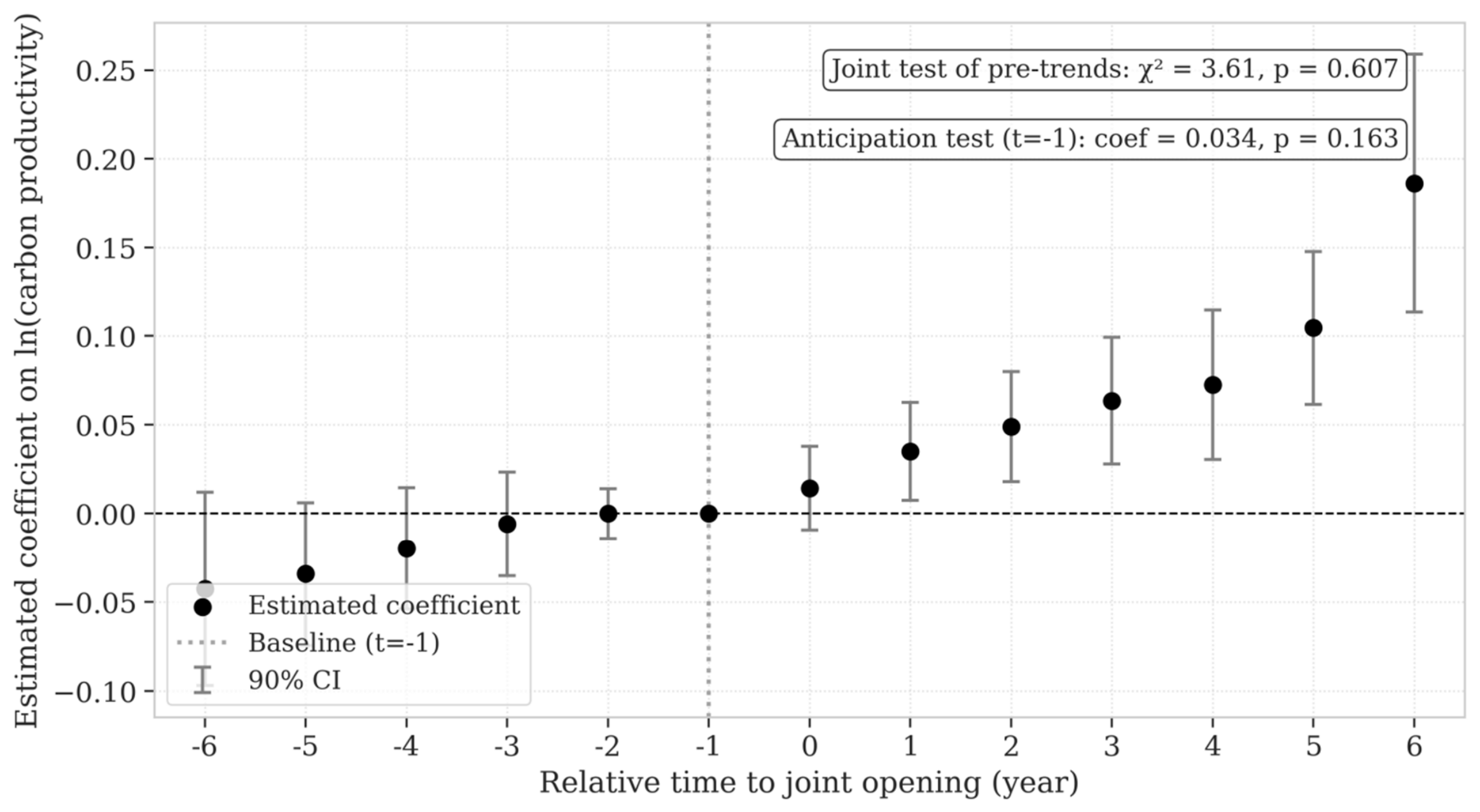
As illustrated in

Table 4. Parallel trend test (the first period before the implementation of the policy (pre1) was used as the base period, and the coefficients were omitted and not listed. ***, **, and * indicate significant at the statistical levels of 1%, 5%, and 10%, respectively).

Variable	lnCP
pre6 and earlier	−0.0424
	−0.0331
pre5	−0.0341
	−0.0244
pre4	−0.0197
	−0.0208
pre3	−0.0059
	−0.0178
pre2	0.0001
	−0.0086
current	0.0143
	−0.0143
post1	0.0351 **
	−0.0167
post2	0.0490 ***
	−0.0188
post3	0.0636 ***
	−0.0217
post4	0.0725 ***
	−0.0256
post5	0.1047 ***
	−0.0263
post6 plus	0.1861 ***
	−0.0442
Control variables	Yes
Urban FE	Yes
Year FE	Yes
Observation value N	4772

and Figure 1, all pre-treatment coefficients spanning pre6 and earlier to pre2 are statistically insignificant and numerically close to zero. The joint Wald test for all pre-policy dummies cannot reject the null hypothesis of parallel pre-trends, verifying that the treated and control cities follow indistinguishable carbon productivity paths before the coordinated rail opening, thus validating the core DID identification assumption.

In the policy contemporaneous year ($k=0$), the coefficient equals 0.0143 and lacks statistical significance, ruling out anticipation effects or immediate policy gains. Significant positive impacts only emerge from the first post-treatment year onward ($\beta =0.0351$, $p<0.05$) and rise monotonically across subsequent periods, reaching 0.1861 for windows six years and later ($p<0.01$). This gradually growing dynamic effect aligns with economic logic: integrating inter-city high-speed rail and urban subway networks, reshaping residents’ travel modal choices, and adjusting urban industrial structures all demand sustained time to materialize the full green benefits of combined transport infrastructure investment.

5.4. Heterogeneity Analysis: The Difference in the Effect of High- and Low-GDP Cities

To examine the heterogeneous effects across cities with different economic development levels, a dynamic grouping strategy was adopted based on the annual cross-sectional mean of GDP under the control of city fixed effects and year fixed effects.

Specifically, the study calculated the cross-sectional average GDP of all sample cities in each year during 2008—2024. For each city and year observation, the city was classified into the high-GDP city group if its annual GDP was higher than the annual cross-sectional mean, and into the low-GDP city group if its annual GDP was lower. This dynamic grouping approach avoids the bias introduced by static full-sample mean grouping, aligns with the panel data structure and two-way fixed-effects specification, and allows us to capture how the joint opening effect varies across cities at different stages of economic development over time.

Table 5. Heterogeneity analysis. (***, **, and * indicate significant at the statistical levels of 1%, 5%, and 10%, respectively).

Variable	(1) Low-GDP lnCP	(2) Low-GDP lnCO2	(3) Low-GDP lnGDP	(4) High-GDP lnCP	(5) High-GDP lnCO2	(6) High-GDP lnGDP
DID	0.0764 *** (0.0268)	−0.0330 * (0.0175)	0.0334 ** (0.0161)	0.0815 *** (0.0259)	−0.0745 *** (0.0180)	0.0207 (0.0159)
SEC	0.0010 (0.0015)	0.0040 *** (0.0013)	0.0052 *** (0.0008)	−0.0002 (0.0016)	0.0050 *** (0.0012)	0.0047 *** (0.0009)
INV	−0.0008 (0.0040)	0.0023 (0.0037)	0.0028 (0.0022)	−0.0055 (0.0041)	0.0141 *** (0.0034)	0.0086 *** (0.0022)
GOV_EXP	0.7189 *** (0.0690)	0.0653 (0.0428)	0.8039 *** (0.0571)	0.5243 *** (0.0647)	0.0635 (0.0411)	0.5764 *** (0.0532)
FDI	0.0041 (0.0041)	−0.0072 ** (0.0033)	−0.0047 ** (0.0019)	0.0033 (0.0038)	−0.0087 *** (0.0030)	0.0005 (0.0018)
FIS	−2.8818 *** (0.2061)	0.0136 (0.1579)	−2.8887 *** (0.1803)	−5.0443 *** (0.2092)	0.2578 (0.1547)	−4.8910 *** (0.1799)
POP	−0.0269 (0.0185)	0.0180 (0.0148)	−0.0080 (0.0096)	0.0373 ** (0.0179)	−0.0349 ** (0.0162)	−0.0126 (0.0094)
Urban FE	YES	YES	YES	YES	YES	YES
Year FE	YES	YES	YES	YES	YES	YES
N	3518	3518	3518	1254	1254	1254

reports the results of heterogeneity regression. There were significant differences in the level of economic development of policy effects. The joint opening has a significant effect on the carbon productivity of high- and low-GDP cities by 1%. Among them, the economic growth promotion effect of low-GDP cities was significant, and the economic growth effect of high-GDP cities was not significant. In terms of carbon productivity improvement, the DID coefficient of high-GDP cities was 0.0815 and 0.0764 for low-GDP cities, both of which were significantly positive at the 1% level, and the carbon productivity improvement effect of cities with high economic development level was stronger. In terms of carbon emission suppression, the DID coefficient of high-GDP cities was −0.0745 and −0.0330 for low-GDP cities, and the emission reduction in high-GDP cities was much greater than that of low-GDP cities. In terms of economic growth, the DID coefficients of both groups of cities were positive, and there was a positive trend of policies promoting the economic development of both types of cities. As shown in

Table 6. The adjustment effect of economic development level. (***, **, and * indicate significant at the statistical levels of 1%, 5%, and 10%, respectively).

Variable	(1) lnCP	(2) lnCO2	(3) lnGDP
DID	0.0736 ***	−0.0351 **	0.0278 **
DID_HIGHGDP	0.0298 **	−0.0579 ***	−0.0026
Control variables	YES	YES	YES
City and year fixed effects	YES	YES	YES

, the results of the moderating effect further verified the above conclusions. The DID_HIGHGDP interaction term was significantly positive in the carbon productivity model and negative in the carbon emission model, but not significant in the economic growth model, indicating that the economic development level mainly positively regulates the emission reduction effect of joint opening, but did not have a significant moderating effect on economic growth. The higher the level of urban economic development, the stronger the effect of the joint opening of high-speed rail and subway systems on improving carbon productivity and inhibiting carbon emissions, and the economic foundation is the key support for amplifying the green and economic effects of policies.

5.5. Mechanism Test: The Moderating Role of Private Car Stock in the Transportation Substitution Effect

The transportation substitution effect was a theoretically plausible channel through which the coexistence of HSR and subway systems might raise urban carbon productivity. The combined low-carbon travel network formed by dual rail systems could provide residents with full-chain low-carbon travel options, potentially reducing reliance on high-carbon modes such as private cars, thereby lowering carbon emissions while sustaining economic growth. In cities with higher private car stock, residents were more dependent on private vehicles on average and had higher travel-related carbon intensity. If the dual rail system displaced private car travel, the marginal carbon productivity gain would be larger in cities with a larger existing car fleet. For this reason, private car stock was used as a moderating variable to test whether the empirical pattern was consistent with the transportation substitution mechanism.

To estimate the moderating effect of private car stock, this study employed the Double/Debiased Machine Learning (DML) framework to estimate an interaction term model. Traditional linear interaction models are prone to biased estimates due to misspecification of the functional form of the control variables. DML, through orthogonalization and cross-fitting, flexibly controlled for high-dimensional nonlinear confounders and yielded unbiased and asymptotically normal interaction coefficients. The model was specified as:

$$lnC{P}_{it}={\theta }_0+{\theta }_{1}DI{D}_{it}+{\theta }_{2}Ca{r}_{it}+{\theta }_3\left(DI{D}_{it}\times Ca{r}_{it}\right)+g\left(W_{it}\right)+{\mu }_i+{\lambda }_t+{\epsilon }_{it}$$

(4)

where $lnC{P}_{it}$, $DI{D}_{it}$, ${\mu }_i$, ${\lambda }_t$, and ${\epsilon }_{it}$ were as defined previously. $Ca{r}_{it}$ represents private car stock, measured alternatively by its natural logarithm and a standardized value to remove scale effects. Also, to be more scientific, this model used the private car growth rate, based 2008, which was computed as:

$$Growt{h}_{it}={\displaystyle \frac{PrivateCa{r}_{it}}{PrivateCa{r}_{i,2008}}}-1$$

(5)

where $PrivateCa{r}_{i,2008}$ is the private car stock of city $i$ in year 2008. For cities without a 2008 observation, the earliest available pre-policy year was used as the base. $g\left(W_{it}\right)$ is a nonlinear function of the high-dimensional control variables that uses the same set as in the baseline regression, which is estimated via random forest. ${\theta }_3$ on the interaction term is the parameter of interest. A significantly positive ${\theta }_3$ indicates that private car stock positively moderates the policy effect, which is consistent with the transportation substitution mechanism.

As reported in

Table 7. Moderating effect of private car stock (the model was estimated using LinearDML with 5-fold cross-fitting and random forest as the first-stage learner. lnCAR: natural logarithm of private car stock; Std.CAR: standardized private car stock; and CGR: private car growth rate, based on 2008 data. ***, **, and * indicate significant at the statistical levels of 1%, 5%, and 10%, respectively).

Variable	Interaction Coefficient	Std. Err.	z-Value	95% CI
lnCAR	0.075 **	0.038	1.981	[0.0001, 0.149]
Std.CAR	0.220 ***	0.042	5.219	[0.137, 0.303]
CGR	−0.010	0.011	−0.892	[−0.033, 0.012]

, the interaction coefficient for lnCAR is 0.075, which is significant at the 5% level. The interaction coefficient for the standardized private car stock is 0.220, which is significant at the 1% level. In contrast, the coefficient for the cumulative growth rate is negative and statistically insignificant. This pattern indicates that the policy effect is closely associated with the stock level of private cars rather than their growth rate. Higher private car stock level is associated with a larger carbon productivity improvement due to dual rail coexistence.

This empirical pattern is consistent with the theoretical expectation that cities with higher car dependence possess greater emission reduction potential through modal shift, and that the combined low-carbon rail network could unlock this potential. The fact that the policy effect depended on the stock level rather than the growth rate suggests that the effect operates mainly through the existing travel structure, rather than through suppressing new car purchases.

Several reasons explain why the growth rate failed to produce a significant moderating effect. First, the growth rate captures annual fluctuations in new car registrations, which are heavily influenced by macroeconomic conditions, fuel prices, and government subsidies for electric vehicles. These short-term shocks introduce substantial noise into the growth rate measure and obscure its relationship with the substitution behavior of existing residents. Second, the growth rate reflects changes at the margin, whereas the substitution potential of rail transit depends on the stock of current private car users who could immediately switch to the newly available rail options. A city with a high growth rate but a low stock has few existing car users to substitute, limiting the emission reduction potential from the modal shift. Third, the growth rate primarily concerns new car buyers, whose travel habits are not yet firmly established; these individuals might adopt rail transit from the outset without experiencing a behavioral switch. Their contribution to the substitution effect thus differed fundamentally from that of long-term car-dependent residents captured by the stock measure. Fourth, the cumulative growth rate of private cars did not produce a significant moderating effect. This null finding might be explained by short-term fluctuations in macroeconomic conditions, fuel prices, and government subsidies for new energy vehicles, all of which introduce noise into the growth rate measure and obscure its relationship with existing residents’ travel behavior.

Importantly, this moderating effect result provides only indirect evidence compatible with the transportation substitution mechanism, and does not constitute direct proof of actual modal shift behavior. Private car stock was correlated with a range of urban characteristics, including city size, economic development level, urbanization rate, infrastructure quality, and commuting demand. The observed stronger effect in high-stock cities could not be exclusively attributed to residents switching from private cars to rail transit.

The mechanism test was further limited by the absence of direct intermediary variables. This study did not include data on metro or HSR passenger volumes, private car usage intensity, travel mode shares, traffic congestion levels, or transport-related fuel consumption. Without these variables, it was not possible to verify whether residents actually reduced car usage or shifted to rail transit after the simultaneous opening of both systems. The interaction between private car stock and the treatment variable could only suggest that cities with more cars exhibit larger carbon productivity gains—an observation consistent with the substitution logic, but not a direct test of behavioral change.

By ruling out estimation bias due to nonlinearities in the high-dimensional controls, the DML approach strengthened the credibility of the observed moderating pattern. Nevertheless, the empirical evidence offered only indirect support for the plausibility of the transportation substitution mechanism, and the mechanism analysis should be interpreted as exploratory rather than confirmatory.

5.6. Placebo Test Result

To validate the robustness of baseline findings, this study employed coarsened exact matching (CEM) as a preprocessing method, followed by re-estimation of the multi-period DID model on the matched sample. CEM, proposed by Iacus, King, and Porro, belongs to the class of Monotonic Imbalance Bounding (MIB) matching methods [43]. Unlike Propensity Score Matching (PSM), CEM does not rely on the correct specification of a propensity score model. Instead, it coarsens each covariate into substantively meaningful intervals and performs exact matching within each coarsened stratum. The core logic is straightforward: researchers define coarsening thresholds for each covariate based on prior knowledge; observations falling into the same coarsened stratum are considered matchable, thereby bounding the maximum allowable imbalance for each covariate ex ante.

CEM offers several notable advantages over PSM. First, PSM belongs to the Equal Percent Bias Reduction (EPBR) class of methods, where balance improvement is only guaranteed on average across repeated samples; a single application may actually increase covariate imbalance. In contrast, as an MIB method, CEM ensures that the imbalance bound for each covariate is predetermined by the researcher, and coarsening one variable has no effect on the imbalance bounds of other variables. Second, CEM eliminates the need to specify a propensity score model, thereby avoiding bias from model misspecification. Third, CEM simultaneously implements common support restriction and matching in a single step, unlike PSM, which requires separate procedures. Fourth, CEM exhibits approximate invariance to measurement error; empirical evidence shows that CEM retains over 95% of matched samples after data perturbation, compared to only approximately 70% for PSM.

Recent policy evaluation studies have increasingly adopted CEM. Zhou, Li, and Wen employed CEM-DID as a robustness check when examining the impact of digital infrastructure on carbon neutrality in Chinese cities, finding that CEM substantially improved model explanatory power while the policy coefficient remained significantly positive [44].

Following these studies, CEM was incorporated as a robustness check alongside baseline DID specification. The procedure involved three steps, including defining coarsening intervals for each covariate based on its distribution, performing exact matching within the coarsened multidimensional space, retaining only strata containing at least one treated unit and one control unit, and re-estimating the DID model on the matched sample. This approach enabled the study to effectively mitigate selection bias and verified that baseline conclusions are not driven by specific model assumptions.

Table 8. CEM-DID (CEM used coarsened exact matching with 4 bins per covariate; standard errors for matching estimates are based on bootstrapped paired differences with 500 replications. ***, **, and * indicate significant at the statistical levels of 1%, 5%, and 10%, respectively).

Variable	Two-Way FE (Baseline)	CEM-DID
DID/ATE coefficient	0.0999 ***	0.4253 ***
Standard error	(0.0265)	(0.0609)
z-value	—	6.98
p-value	—	0.0000
95% CI	—	[0.299, 0.538]
Effective sample (weighted)	4772	625
Covariates balanced (std. diff. < 10%)	—	Partial
City FE	YES	YES
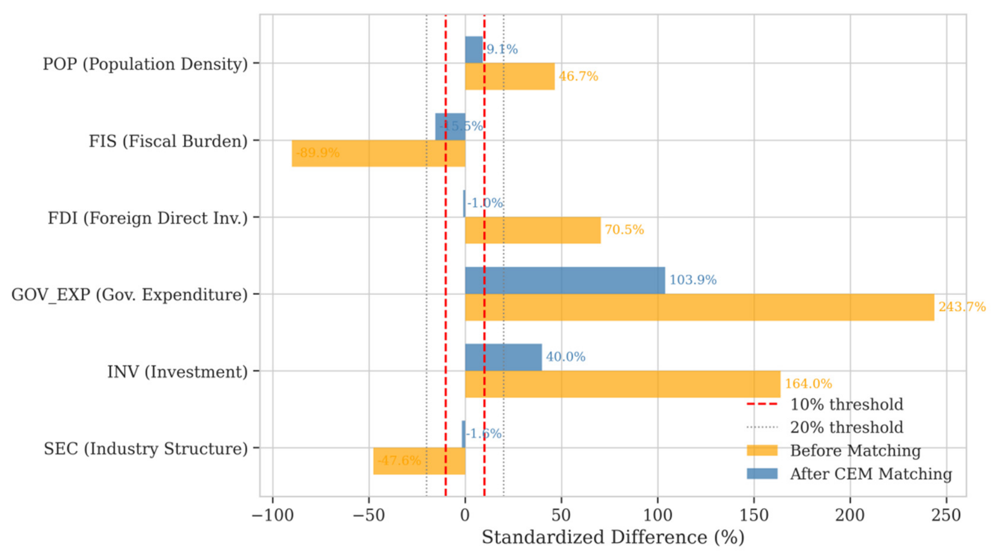
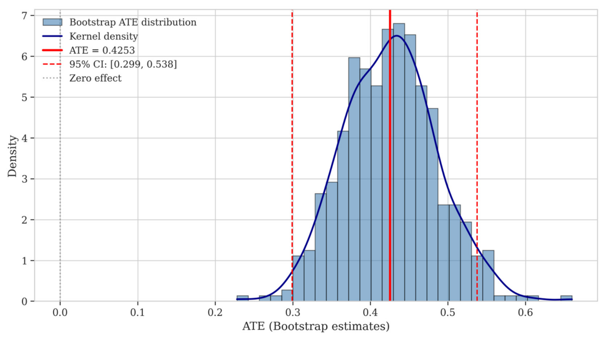
Year FE	YES	YES

reports the CEM-DID estimation results. The CEM-DID balance diagnostics and bootstrap distribution are shown in Figure 2 and Figure 3, respectively. To address potential selection bias, the study first estimated an unconditional CEM-DID model. The estimated ATE is 0.4253 and statistically significant. However, because the unconditional CEM estimate did not further adjust for remaining covariate imbalances after matching, and the effective sample size decreased substantially, this large estimate should be interpreted as a local average treatment effect for the matched subsample. The conditional CEM-TWFE model, which includes lagged covariates and two-way fixed effects, produced a coefficient of 0.0648, as shown in

Table 9. Conditional CEM-TWFE DID (single joint policy dummy, matched sample with lagged covariates. ***, **, and * indicate significant at the statistical levels of 1%, 5%, and 10%, respectively).

Variable	Coefficient (Standard Error)
Intercept	−1.7031(2.191)
DID (joint HSR and subway system policy dummy)	0.0648 ** (0.0284)
sec_lag1	0.0032(0.0044)
inv_lag1	0.0122(0.0149)
gov_exp_lag1	0.1190(0.1542)
fdi_lag1	−0.0025(0.0113)
fis_lag1	−1.6874 * (0.9181)
lnpop_lag1	0.0172(0.0269)
Model statistics
Within R2	0.2495
Total observations	1196
Number of cities	157
Number of CEM matching strata	39
City and year fixed effects	YES

, which is closer to the baseline DID estimate (0.0999) and remains statistically significant at the 5% level. This conditional result provides more comparable evidence for the baseline specification and confirms the positive direction of the effect. It confirms that the joint policy still exerts a significant positive impact after controlling for remaining covariate imbalances, which supports the robustness of the core conclusion. The difference between the unconditional and conditional CEM estimates stems from two sources. First, the unconditional estimate did not further control for confounding factors within the matched sample. Second, strict exact matching dropped a large number of off-support observations, and the unconditional result reflects a local average treatment effect for specific comparable subgroups. The conditional estimate with lagged controls is more comparable to the baseline model setting and serves as the core robustness result of the CEM test.

This conditional specification estimates the net effect of dual rail coexistence on the matched sample, and was not designed to decompose standalone HSR effects, standalone subway effects, or their additional joint impact.

Taken together, the full set of CEM-DID tests consistently supports the core baseline conclusion, which means that the joint opening of HSR and subway systems significantly improves urban carbon productivity.

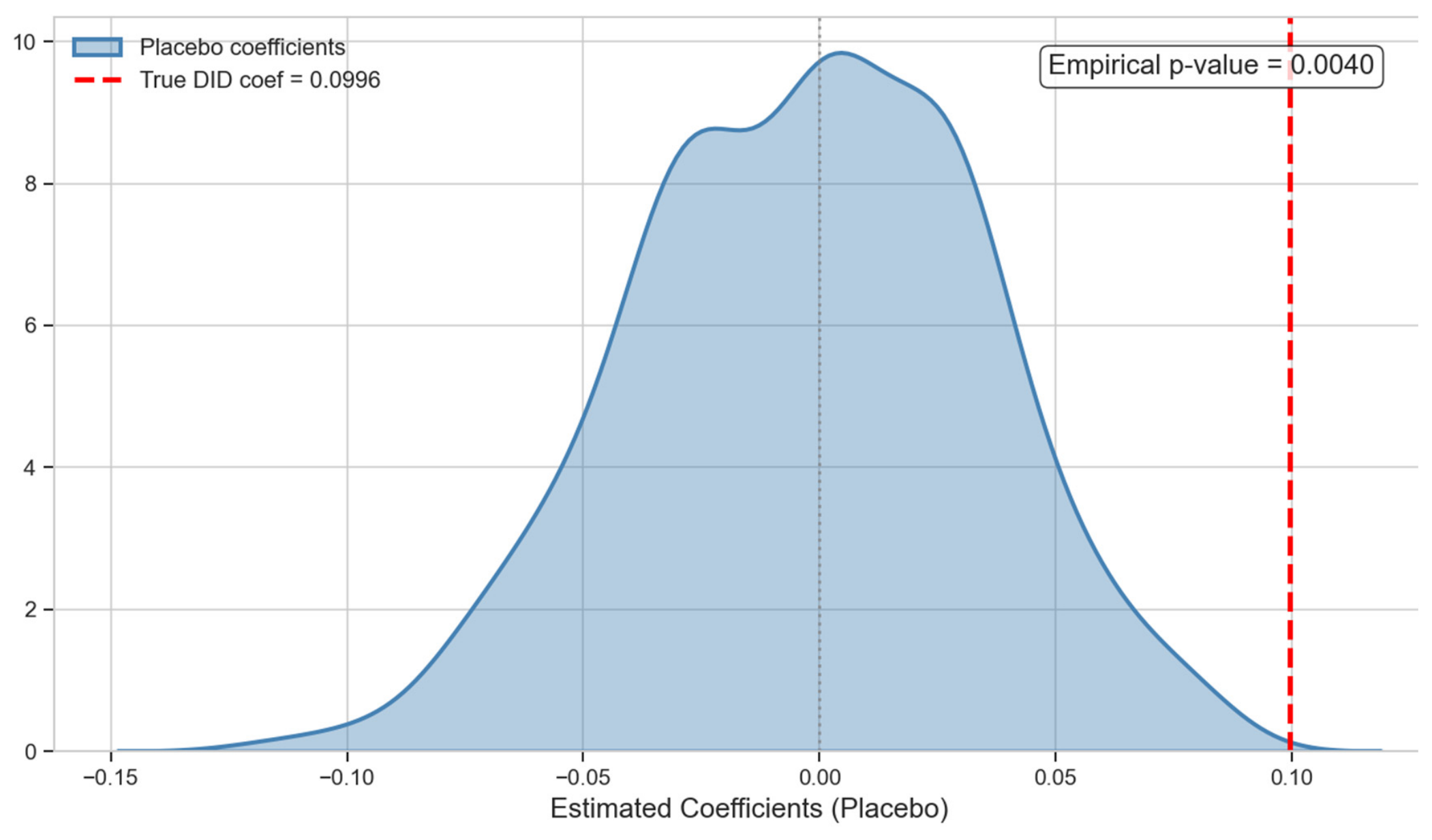
To exclude the interference of unobservable random shocks on baseline regression results and verify the validity and robustness of the estimated net policy effect, this paper conducted a placebo test via random assignment of treatment cities and policy implementation years. The test design strictly matched the specification of the baseline regression. Virtual treatment cities were randomly selected from all 287 sample cities and assigned a random policy implementation year between 2008 and 2024 to each selected city to construct a false DID interaction term, which fully preserved the multi-period panel structure. All simulated regressions adopted the two-way fixed-effect framework, an identical set of control variables, and city-level clustered standard errors as the baseline regression, with only the core DID variable replaced. The above random simulation procedure was repeated 500 times and the reliability of the baseline estimates was judged by comparing the distribution of the true policy coefficient and placebo coefficients.

The results in

Table 10. Placebo test (the empirical p-value is defined as the proportion of samples where the absolute value of the placebo coefficient exceeds that of the real coefficient among 500 simulations. Both the baseline regression and all placebo regressions controlled for city fixed effects, year fixed effects, and six control variables. ***, **, and * indicate significant at the statistical levels of 1%, 5%, and 10%, respectively).

Indicator	Estimated Value
DID	0.0999 *** (0.0273)
T-value	3.6593
Within R2	0.7894
Control variables	Yes
Total number of random simulations	500
Mean of placebo coefficients	0.0000
Std of placebo coefficients	0.0375
Median of placebo coefficients	0.0020
Empirical p-value	0.0060

show that the mean of placebo coefficients generated by 500 random simulations is close to zero, and the overall distribution is concentrated around zero, which indicates that randomly assigned fictitious policies exerted no systematic economic impact. The true DID estimate equaled 0.0999 and deviated substantially from the placebo distribution. The corresponding empirical p-value is 0.0060, meaning the null hypothesis that the policy effect was driven by random noise could be rejected at the 1% significance level. The placebo coefficient distribution is visualized in Figure 4.

These results fully validate the robustness of the baseline findings. The policy-induced promotion effect on urban carbon productivity was not derived from unobservable random shocks, measurement errors, or omitted variables, but reflects a clean and robust causal effect. Throughout the placebo simulation, the multi-period panel structure and two-way fixed-effect setup were fully retained, and the control variable set remained consistent with the baseline regression, which further guarantees the internal validity of this robustness test.

5.7. Robustness Test Result

To verify the reliability of the baseline regression results and mitigate potential biases from measurement errors, sample selection issues, and exogenous shocks, this study conducted five complementary robustness tests. All specifications retained the two-way fixed effects and city-level clustered standard errors consistent with the baseline model. The test procedures were as follows. The first test was the baseline regression, which used a full-sample regression with original variables as the reference benchmark. The second test applied GDP deflation and control variable normalization. Nominal GDP was deflated using the 2008-based GDP deflator to eliminate inflation effects, and all continuous control variables were normalized via the Min–Max method to remove dimensional interference. The third test excluded epidemic period samples. Samples from 2020 to 2024 were excluded to rule out exogenous shocks from COVID-19-related travel restrictions and economic disruptions. The fourth test excluded municipality samples. The four municipalities, including Beijing, Shanghai, Tianjin, and Chongqing, were excluded to eliminate bias from extreme and institutionally distinct samples. The fifth test applied double exclusion. Both epidemic period samples and municipality samples were excluded to address superimposed exogenous and extreme sample interference.

Table 11. Robustness test. (***, **, and * indicate significant at the statistical levels of 1%, 5%, and 10%, respectively).

Variable	(1)	(2)	(3)	(4)	(5)
DID	0.0999 ***	0.1055 ***	0.0781 ***	0.0864 ***	0.0672 ***
	(0.0265)	(0.0224)	(0.0208)	(0.0259)	(0.0201)
Control variables	Yes	Yes	Yes	Yes	Yes
Urban fixed effect	Yes	Yes	Yes	Yes	Yes
Year fixed effect	Yes	Yes	Yes	Yes	Yes
Observations	4772	4772	3457	4708	3409
Within-R2	0.7960	0.8087	0.7687	0.8008	0.7722

shows that all the robustness tests support the core conclusion. In those tests, the DID coefficients remain positive and significant at the 1% statistical level, and no sign reversal, loss of significance, or notable decline occurs in any test. This directly proves that the core conclusion, namely that the joint opening of high-speed rail and subway systems significantly improves urban carbon productivity, was not driven by data measurement methods, sample selection, or exogenous shocks.

This research constructed a unified two-way fixed-effects regression framework. The specification incorporated three core binary indicators: a dummy variable marking high-speed rail opening, a dummy variable marking subway system opening, and their cross-product interaction term hsr × sub. This interaction term quantified the additional joint effects beyond the sum of individual impacts generated when cities operate both transit systems simultaneously. The analysis retained the complete set of control variables adopted in the baseline regression, and all standard errors were clustered at the city level.

As shown in

Table 12. Tests for joint effects of HSR and subway systems beyond individual impacts (the bootstrap test used 500 replications and reported one-sided test results; severe multicollinearity among HSR, subway systems, and interaction terms caused frequent non-convergence during random resampling, so the delta method based on full-sample regressions serves as the robust benchmark for coefficient difference inference. ***, **, and * indicate significant at the statistical levels of 1%, 5%, and 10%, respectively).

Variable	Estimates
HSR	−0.0053
	(0.0167)
Subway	−0.1092
	(0.0776)
HSR × subway interaction (hsr × sub)	0.2016 ***
	(0.0747)
Control variables	Yes
City fixed effects	Yes
Year fixed effects	Yes
Wald test (hsr × sub = 0) χ2 statistic	7.27 ***
Bootstrap difference test	0.0092 **
Delta test	0.0093
Observations	4772
Number of cities	287
Within-R2	0.7785

, the standalone HSR coefficient equals −0.0053 and carries no statistical significance. The standalone subway system coefficient reached −0.1092, and this estimate also lacks significance. In contrast, the interaction term produced a positive coefficient of 0.2016. This estimate is statistically significant at the 1 percent level.

A Wald test was implemented to verify whether the joint effects differed from the simple linear sum of the two transit policies. The test established a null hypothesis that the interaction coefficient equaled zero. If the hypothesis held, the total effect of dual transit only equaled the added value of the standalone HSR and subway system effects. The test generated a chi-squared statistic of 7.27 with a p-value of 0.007. The result rejects the null hypothesis at the 1 percent level. The data confirm that simultaneous operation of HSR and subway systems generates an additional combined effect beyond their separate contributions. The total effect of dual rail operation in the unified interaction model was calculated as $\left({\beta }_{hsr}+{\beta }_{sub}+{\beta }_{hsr\times sub}\right)$, which is equal to about 0.0871. This value is close in magnitude and identical in direction to the baseline DID coefficient of 0.0999. The small numerical gap stems from different definitions of control groups. The baseline DID model classified cities with only HSR or only a subway system into the control group. The unified interaction model took cities with no rail infrastructure as the pure control group and separately estimated the standalone effect of each single transit system. Despite this grouping difference, both estimates are significantly positive at the 1 percent level, which supports the robustness of the core baseline conclusion. Importantly, the identified additional joint effect is a statistical result at the city level. It reflects that the combined impact of the two systems exceeds the simple sum of their individual effects, but does not directly represent operational synergy at the station level.

5.8. Robustness Check for Staggered DID: Goodman–Bacon Decomposition

Given that HSR and subway system openings occurred in different years across cities, the study featured a typical staggered adoption design. To assess whether the conventional two-way fixed-effect (TWFE) estimator was contaminated by heterogeneous treatment effects, the decomposition proposed by Goodman–Bacon was applied [45]. This method decomposed the aggregate TWFE estimator into a weighted average of all valid 2 × 2 DID pairwise comparisons, and identified which comparisons may carry problematic weights or introduce estimation bias. Notably, this decomposition was performed on the level value of carbon productivity, while the baseline regression used the natural logarithm form of carbon productivity. The two sets of results have different measurement units and are not directly comparable in numerical magnitude. The core function of the decomposition is to diagnose the direction of treatment effects and the structure of weight allocation, rather than matching the numerical scale of the baseline log-form estimate. Because the decomposition’s primary function is to diagnose the direction of treatment effects and the structure of weight allocation, rather than to provide a magnitude estimate comparable to the baseline log-form coefficient, the use of level carbon productivity did not undermine the diagnostic validity of the decomposition.

Table 13. Goodman–Bacon decomposition.

No.	Comparison Type	2 × 2 DID Estimate	Normalized Weight
1	Treated vs. Never-treated	2.9296	0.1323
2	Treated vs. Never-treated	1.8325	0.2396
3	Treated vs. Never-treated	1.0759	0.125
4	Early vs. Late (pre-late window)	2.1084	0.0372
5	Late vs. Early (post-early window)	0.7203	0.1265
6	Early vs. Late (pre-late window)	2.4267	0.0462
7	Late vs. Early (post-early window)	0.0009	0.0943
8	Early vs. Late (pre-late window)	1.5314	0.0586
9	Late vs. Early (post-early window)	0.6416	0.1405
—	Total	—	1.0002

reports the Goodman–Bacon decomposition results. The baseline aggregate TWFE coefficient equals 1.6730, while the weighted sum of all nine separate 2 × 2 DID estimates was 1.4225. The two values share identical positive signs, indicating that heterogeneous dynamic effects only caused mild attenuation of the overall policy effect, rather than reversing the core result.

Notable numerical gaps exist between individual subsample 2 × 2 estimates and the full-sample baseline coefficient. These gaps are explained systematically from three dimensions: comparison type, sample comparability, and normalized weight distribution.

First, comparisons between treated cities and never-treated cities delivered the most reliable identifying variation. No previously treated units appeared in the control groups within this category, so staggered adoption bias was absent. The three corresponding local estimates ranged from 1.0759 to 2.9296, which are all larger than the baseline value. Their combined normalized weight reached 0.4969 (49.69%). The larger point estimates arose because this subsample only included cities with limited initial rail infrastructure, which generated greater marginal policy gains. This category occupied nearly half of the total weights and dominated the sign of the final weighted average.

Second, comparisons that took early-adopting cities as treated units and not-yet-treated late cohorts as the controls (pre-late window) carried a total normalized weight of 0.1420. Their 2 × 2 estimates fell between 1.5314 and 2.4267, which is also above the baseline magnitude. The control units in this group had not yet received rail services during the observation window, so sample comparability remained sound. The small weight share limited their overall influence on the aggregate outcome.

Third, comparisons that treated late-opening cities as treated units and already-treated early cities as controls (post-early window) accounted for a total normalized weight of 0.3613. Local estimates in this group ranged from 0.0009 to 0.7203, which are all far smaller than the baseline coefficient. Comparability was weakened here: early cities had already gained long-term benefits from rail construction, which narrowed outcome gaps between treatment and control units and created downward estimation bias. Even with a weight share above one-third, these attenuated small values failed to reverse the positive direction of the weighted aggregate.

Taken together, the decomposition results clarify the scale difference, weight allocation, and comparability features of every subsample estimate relative to the baseline TWFE coefficient. While contaminated late-versus-early comparisons produced downward-biased small estimates, clean treated-versus-never-treated contrasts held dominant weights and maintained positive signals. Heterogeneous treatment effects only slightly reduced the economic scale of the aggregate estimate, without changing the core economic implication of the analysis.

5.9. Machine Learning Supplementary Verification: Based on DML Causal Forest

To complement the baseline parametric identification and verify whether the core conclusion depended on linear functional form assumptions, the causal effect of dual rail coexistence was estimated using a double machine learning (DML) causal forest estimator. Implemented via the Causal Forest DML module in the Python econml package, this approach integrated two core strengths: the double robustness of DML against confounding bias, and the flexibility of generalized random forests in capturing heterogeneous treatment effects without preset functional forms.

To align with the identification strategy of the baseline two-way fixed-effects DID model, city and year fixed effects were first absorbed by applying within-transformation to the outcome variable (carbon productivity) and all time-varying covariates. The binary treatment variable was retained in its original 0/1 integer form. The DML procedure was then implemented with 5-fold cross-fitting. For each fold, auxiliary prediction forests were trained on the remaining folds to residualize both the outcome and treatment variables against all observable confounders. This cross-sample residualization eliminated overfitting bias caused by using the same sample for both confounder adjustment and effect estimation, and ensured double-robust causal identification. The main estimation model employed 1000 decision trees with honest splitting to enhance out-of-sample reliability.

For statistical inference, a city-level clustered bootstrap procedure with 100 replications was adopted to compute standard errors and construct 95% percentile confidence intervals. This strategy explicitly accounted for within-city serial correlation in panel data, and was methodologically consistent with the city-clustered robust standard errors used in the baseline DID regression.

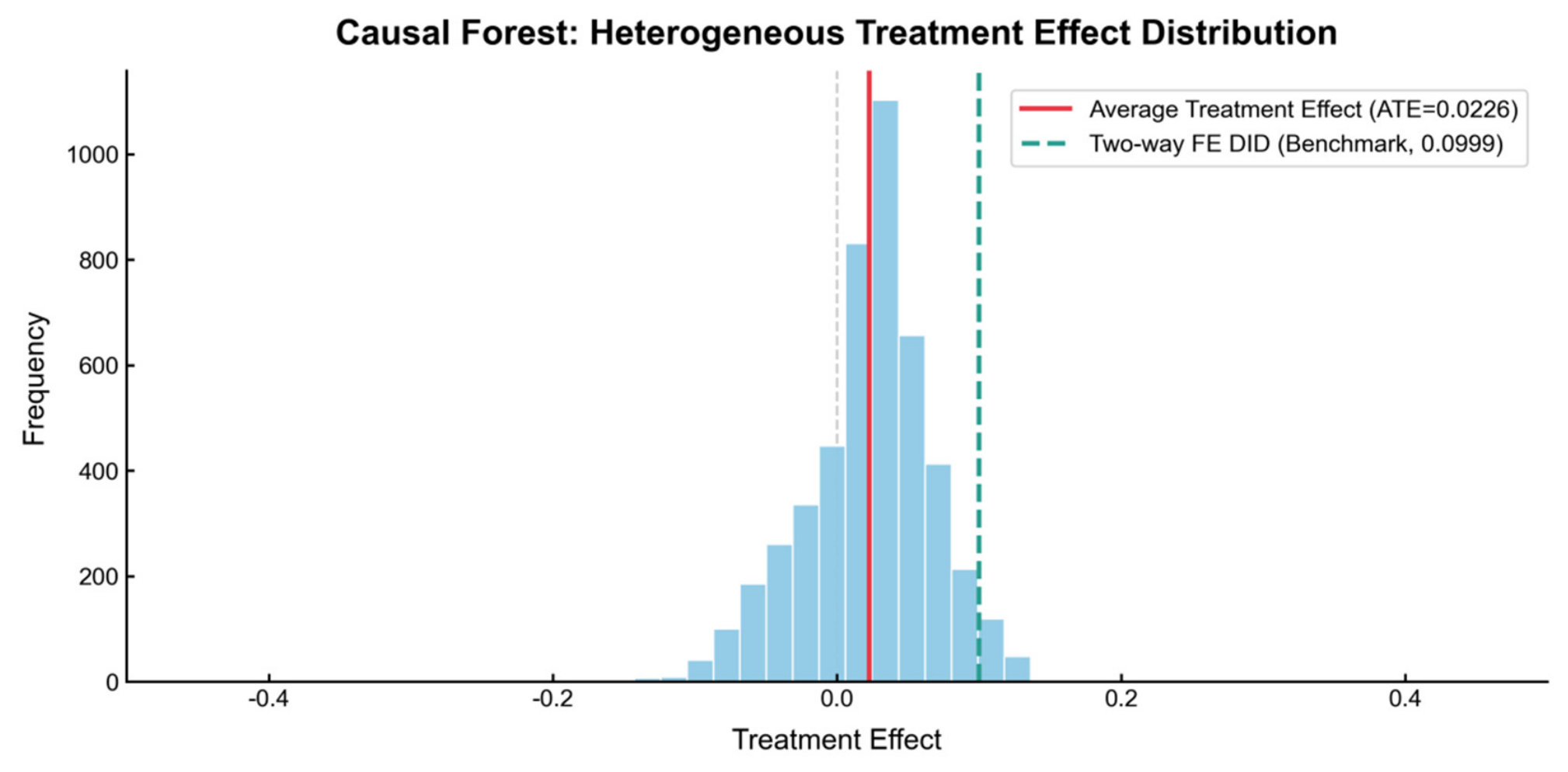
As shown in

Table 14. Comparison of parametric DID and nonparametric causal forest estimates (the causal forest estimates were based on two-way fixed-effects absorption, with standard errors and 95% confidence intervals calculated via 100-replication city-level clustered bootstrap. ***, **, and * indicate significant at the statistical levels of 1%, 5%, and 10%, respectively).

Method	Effect Value	Standard Error	95% Confidence Interval
DID	0.0999 ***	0.0265	—
Causal Forest (ATE)	0.0226 ***	0.0092	[0.0074, 0.0429]
Causal Forest (ATT)	0.0251 ***	0.0095	[0.0107, 0.0479]

, the causal forest yielded a full-sample average treatment effect (ATE) of 0.0226 and an average treatment effect on the treated (ATT) of 0.0251. Both estimates are statistically significant at the 1% level, confirming that the coexistence of HSR and subway systems exerts a positive net causal effect on urban carbon productivity, even under nonparametric assumptions. This finding is qualitatively consistent with the baseline DID results, providing supportive evidence for the causal validity of the core conclusion. A notable quantitative gap exists between the parametric DID estimate and the nonparametric causal forest estimates, with the latter having approximately one-quarter the magnitude of the former. This discrepancy was theoretically expected and methodologically explicable, and does not indicate instability of the core finding. Four key factors drove the magnitude difference. First, the two methods relied on different functional form assumptions. The TWFE DID model is a parametric specification that assumes linear covariate impacts and homogeneous treatment effects across all cities. Its estimate captures not only the pure net treatment effect, but also linear variation in outcomes correlated with observable city characteristics. In contrast, the DML causal forest is a nonparametric estimator that allows for flexible nonlinear relationships between covariates and carbon productivity. It removes confounding variation more thoroughly through cross-fitted residualization, and isolates only exogenous variation in treatment status to estimate the pure net causal effect. Second, a two-stage debiasing procedure was applied in the causal forest analysis. City and year fixed effects were first removed via within-transformation, and residualized confounders were further adjusted through cross-fitting. This double debiasing process absorbed more systematic variation in the outcome variable, which produced a more conservative estimate of the pure treatment effect. Third, the two estimators identified different weighted average parameters. Under the staggered DID design, the TWFE estimator assigned larger weights to cohorts that received treatment earlier and had longer post-policy observation periods. Since treatment effects grew gradually over time, as shown in the dynamic event study results, cohorts with longer exposure windows contributed larger effect sizes to the weighted average. The causal forest, by contrast, estimated individual treatment effects for each observation and aggregated them with approximately equal weights, producing a smaller overall average that reflected the full-sample effect distribution more evenly. Fourth, the two methods served different research purposes and carried different evidentiary weight. The TWFE DID is the baseline specification of the study, and its estimate provides the benchmark magnitude of the overall policy impact. The causal forest functioned as a robustness check that verified the existence and direction of the causal effect under weaker functional form assumptions. It was not intended to replace the baseline estimate as the reference effect size.

Taken together, despite the substantial difference in point estimates, both methods consistently identified a positive and statistically significant effect of dual rail coexistence on urban carbon productivity. The qualitative robustness of the core conclusion did not depend on specific functional form settings. The baseline TWFE estimate remained the primary reference for the economic magnitude of the policy effect, while the causal forest result provided supplementary support for the causal interpretation of the relationship. These differences in magnitude were expected because the two estimators relied on different assumptions and identified different weighted averages of treatment effects. The causal forest results are therefore viewed as confirmatory evidence of a positive causal relationship, rather than as an alternative quantification of the effect size.

As shown in Figure 5, the magnitude of the causal forest estimates was smaller than that of the baseline parametric DID estimate, which was theoretically expected and methodologically reasonable. The parametric DID model imposed assumptions of homogeneous treatment effects and linear covariate impacts, and its estimate captures both the net causal effect and linear confounding variation associated with city characteristics. In contrast, the DML causal forest relaxed these restrictive assumptions because it allowed for nonlinear relationships between covariates and outcomes, as well as heterogeneous treatment effects across cities, and removed confounding variation more rigorously through cross-fitted residualization, thus producing more conservative estimates of the pure net causal effect.

5.10. Discussion

This study employed a staggered DID design to identify the causal effect of co-existing HSR and subway systems on urban carbon productivity. Given that the timing of rail transit openings varied across cities, the study explicitly addressed methodological concerns regarding TWFE estimators under staggered adoption with heterogeneous treatment effects. To assess the validity of TWFE estimates, Goodman–Bacon decomposition was applied, which expresses the TWFE estimator as a weighted average of all possible 2 × 2 DID comparisons. The decomposition results indicated that while some timing-based comparisons might have introduced modest heterogeneity bias, they did not reverse the sign or materially alter the overall conclusion.

The Callaway–Sant’Anna group-time ATT estimator and the Sun–Abraham interaction-weighted estimator offered additional robustness against treatment effect heterogeneity by explicitly avoiding the use of already-treated units as controls [46,47]. However, these estimators required a balanced panel structure with sufficient pre-treatment periods and multiple distinct treatment cohorts. In the present dataset, the panel was unbalanced, with varying numbers of pre-treatment periods across cities, and the number of distinct treatment cohorts was small (three main cohorts). Applying these estimators to the current sample led to near-singular design matrices and unstable standard errors. Given that the Goodman–Bacon decomposition already demonstrated that the TWFE estimate was not driven by problematic comparisons, with clean treated-versus-never-treated comparisons carrying a dominant weight (49.69%) and all subsample estimates sharing the same positive sign, the staggered DID with two-way fixed effects was retained as the primary specification. Future research with longer and more balanced panel data could apply these advanced estimators to further characterize treatment effect heterogeneity across cohorts and over time.

The conclusion of this paper does not rely on a single model setting, but has stable credibility and explanatory power under the dual support of prediction verification and causal inference. Furthermore, in a related study, a recent investigation on Jiangsu Province using an interpretable XGBoost–SHAP framework also confirmed significant spatial heterogeneity in energy-related carbon emissions, with GDP, nighttime light intensity, and built-up land expansion identified as the dominant drivers exhibiting distinct nonlinear thresholds and synergistic interaction effects. This parallel evidence from a different regional context and methodological approach reinforces the broader relevance of machine learning-enhanced analysis for understanding the determinants of carbon emissions [48].

A further limitation concerns the definition of the treatment variable. The DID indicator captured only whether a city had both systems operating, not the degree of physical or operational linkage between them. Thus, the positive effects estimated in this study should be attributed to the co-location of the two rail modes, not to station integration, seamless transfers, or high intermodal ridership. Future research with detailed station-level data could examine whether operational integration strengthens or weakens the estimated effects.

6. Conclusions

Based on Chinese city-level panel data from 2008 to 2024, this study employed a multi-period DID design, complemented by causal forest for nonparametric inference and double machine learning for interaction effect estimation, to examine the impact of the joint opening of HSR and subway systems on urban carbon productivity. Employing a staggered difference-in-differences framework with two-way fixed effects, the study delivers a baseline estimate showing that the joint operation of HSR and subway systems generates a significant positive impact on urban carbon productivity, lifting the level in treated cities by roughly 10.51% on average compared with untreated counterparts. This core conclusion, a positive effect, is qualitatively supported by a comprehensive set of robustness checks, including parallel trend validation, placebo permutation tests, CEM-DID estimation, and multiple sample exclusion strategies. Although the estimated effect sizes varied across methods, all alternative specifications yielded coefficients with the same positive sign and statistical significance. As a nonparametric complement to the parametric baseline specification, causal forest estimates produced smaller yet consistently positive and statistically significant effect sizes, which corroborated the causal nature of the core relationship under weaker functional form assumptions. Heterogeneity analysis based on dynamic GDP grouping revealed that high-GDP cities experienced stronger emission reductions, while low-GDP cities benefited more from the economic growth side of carbon productivity. The mechanism analysis showed that the positive interaction between private car stock and the treatment variable was consistent with the transportation substitution logic. However, this evidence was indirect, as the study did not include direct intermediary variables such as rail passenger volumes, private car usage intensity, or travel mode shares. Therefore, the mechanism results should be interpreted as suggestive and exploratory, rather than as a confirmed test of actual modal shift behavior. This study reveals the spatial symmetric complementarity embedded in the co-location of HSR and subway systems. Although effect magnitudes fluctuated asymmetrically across different identification strategies, the qualitative direction of the positive causal relationship remained symmetric. This directional symmetry offers a new conceptual perspective for understanding the environmental and economic effects of multi-level rail transit.

6.1. Policy Recommendations

Based on the empirical findings, policy formulation should consider the matching degree between dual rail layout and urban development levels, and avoid one-size-fits-all promotion across cities. For high-GDP cities, priority could be given to improving the coverage of both HSR and subway systems, and optimizing the connection between inter-city and urban rail transit. These cities had stronger emission reduction effects under dual rail coexistence, which indicates that they had the economic foundation and commuting demand to translate rail transit investment into actual carbon reduction gains. For low-GDP cities, rail transit construction should be promoted step by step. Priority should be given to improving the connectivity between HSR and existing urban public transport, and supporting the development of local low-carbon industries. Subway system construction should not be launched blindly. These cities benefit more from the economic growth dimension of carbon productivity, which means that transport investment should balance economic development and emission reduction, and excessive rail construction that increases local fiscal pressure should be avoided. In general, cities should promote the coordinated layout of inter-city and urban rail transit according to their own development stages, expand the coverage of green travel networks, and promote the improvement of urban carbon productivity.

6.2. Limitations

Several limitations of this study should be acknowledged, which are discussed in the order of the empirical workflow: variable construction, treatment definition, estimation methodology, mechanism identification, and external validity.

First, regarding the measurement of carbon productivity, the ratio of GDP to total CO₂ emissions was used as the primary indicator. While this single-factor measure has been widely adopted in the literature, it did not account for other production inputs such as labor and capital. Moreover, although a deflation robustness check was conducted, the main analysis relied on nominal GDP values. Future research could employ total-factor carbon productivity estimated through DEA or stochastic frontier analysis to provide a more comprehensive measure that incorporates multiple inputs and addresses inflationary effects more systematically.

Second, concerning the definition of the treatment variable, the DID indicator was coded as 1 when a city had both HSR and subway systems in operation. This definition captured only the co-location of the two infrastructures at the city level. It did not measure operational integration, such as physical connections between subway stations and HSR stations, transfer times, service coordination, or actual intermodal passenger flows. Therefore, the positive effects estimated in this study should be attributed to the simultaneous availability of the two rail modes, rather than to seamless intermodal connectivity, station-level integration, or strong operational synergy. Future research could incorporate station-level variables to assess whether actual physical and operational integration amplifies or modifies the estimated effects, including the distance between subway and HSR stations, scheduled transfer time, network centrality, or intermodal ridership data. Furthermore, the symmetry discussed in this paper was strictly confined to city-level co-location of the two rail systems. It did not cover physical connections, schedule coordination, or actual transfer passenger flows between HSR and subway stations. Future research could utilize station-level data to further examine whether operational integration strengthens or weakens the spatial symmetric effects observed in this study.

Third, the estimated effect size varied considerably across alternative identification strategies. The baseline two-way fixed-effects DID model yielded a coefficient of 0.0999. The unconditional CEM-DID estimate was substantially larger (0.4253), while the conditional CEM-TWFE estimate with lagged covariates produced a coefficient of 0.0648. The nonparametric causal forest estimates (ATE = 0.0226, ATT = 0.0251) were smaller but remained statistically significant. These numerical differences arose because each method relied on different functional form assumptions, weighting schemes, and sample compositions. For instance, the unconditional CEM-DID estimate reflected a local average treatment effect for the matched subsample after dropping many off-support observations, and it did not further adjust for remaining covariate imbalances. The causal forest, by relaxing linearity assumptions and applying cross-fitting, removed confounding variation more rigorously and thus produced more conservative point estimates. Consequently, while the qualitative conclusion—a positive effect—was consistently supported across all specifications, the exact magnitude of the effect should be interpreted with caution and should not be treated as a fixed or universal parameter. The baseline DID estimate remained the primary reference for the economic magnitude, but its numerical value was not invariant to model choice.

Fourth, the positive interaction between private car stock and the DID variable provided indirect evidence consistent with the transportation substitution interpretation. This finding aligned with the theoretical prediction that cities with greater car dependence would exhibit stronger emission reduction potential. However, the analysis relied on the stock measure as a proxy for substitution potential, rather than on direct observations of modal shift. Furthermore, the growth rate of private cars did not show a significant moderating effect; this result is possibly due to short-term fluctuations in macroeconomic conditions, fuel prices, and new energy vehicle policies, which introduced noise into the growth rate measure.

More importantly, the mechanism test did not include direct intermediary variables such as metro or HSR passenger volumes, private car usage intensity, travel mode shares, traffic congestion levels, or transport-related fuel consumption. Without these variables, the study could not verify whether residents actually reduced car usage or shifted to rail transit after the opening of both systems. The interaction analysis could only suggest that cities with higher car stock experienced larger carbon productivity gains—an observation that was consistent with the substitution hypothesis but did not constitute a direct test of behavioral change. Future research could strengthen the mechanism test by incorporating the above-mentioned intermediary variables, which would allow for a more direct assessment of whether actual modal shifts occurred and how much they contributed to the observed carbon productivity improvements.

Fifth, the indirect mechanisms of network collaboration and industrial structure upgrading, although discussed at the theoretical level, were not empirically examined due to data limitations. These pathways may play important roles over the long term. Future research with more detailed industrial and firm-level data could investigate these indirect effects more thoroughly.

Sixth, regarding the staggered DID estimation, the Goodman–Bacon decomposition was used as the primary diagnostic tool for heterogeneous treatment effects. The decomposition was performed on the level of carbon productivity, while the baseline regression used the logarithmic form. This inconsistency arose because the decomposition required outcome variables in their original units to preserve the linear additive property of its weighting scheme; using log-transformed outcomes would have broken this property and made the weight interpretation economically ambiguous. The decomposition results were therefore used only to diagnose the sign and weight distribution of subsample comparisons, not to provide a magnitude reference comparable to the baseline log-form coefficient. The Callaway–Sant’Anna and Sun–Abraham estimators were not applied because the unbalanced panel structure and the limited number of treatment cohorts prevented reliable estimation of standard errors. Future research with longer and more balanced panel data could employ these advanced estimators to provide a more refined characterization of treatment effect heterogeneity across cohorts and over time.

Finally, this study is based exclusively on Chinese city-level data. Given the heterogeneous institutional backgrounds across countries, the findings may not be directly generalizable to other national contexts. Comparative studies across different institutional settings would be valuable for assessing the external validity of the conclusions.