1. Introduction
Metallurgy is one of the oldest human activities; metallurgy s became in a qualified work [
1,
2,
3,
4,
5]. At the beginning only metals with a low fusion temperature were possible to produce due to the limited capacity of heat generation [
3,
4,
5,
6,
7,
8,
9,
10]. Furthermore, steel was difficult to produce due to oxidation and reduction phenomena when heated until melting [
5,
6,
7,
10,
11,
12,
13,
14]. The techniques have been improved for thousands of years [
15,
16,
17,
18,
19,
20]. Nowadays, the variety of tools and components made with metallic materials is huge [
3,
4,
5]; and the need for better-quality steel products is evident. Many mechanical components are made with steels due to their extraordinary strength and resistance properties [
1,
2,
3,
4,
5,
6,
19,
20,
21,
22,
23,
24,
25,
26,
27]. Unfortunately, cast-iron, pig-iron and different kind of scraps are mixed with undesirable metals, residues and contaminants called inclusions [
11,
12,
13,
14,
15,
21,
22,
28,
29,
30,
31,
32]. These inclusions can be metallic or non-metallic and must be removed as much as possible to satisfy the standards of industrial production [
10,
11,
12,
13,
14,
15,
16,
21,
22,
28,
29,
30,
31,
32,
33,
34,
35,
36,
37]. Metallurgical industries are complex companies with all kind of problems from organization, logistics, administration and also engineering; consequently, many areas such as physics and mathematics are applied to solve metallurgical problems including topics related to heat and mass transfer and fluid flow analysis in order to find the best, the quickest and the cheapest approach to heating, casting, solidifying, manufacturing, processing and avoiding mechanical deformations, chemical composition problems, etc. Additionally, many authors have developed models to create metallic grain structures with properties [
3,
4,
5,
6,
7,
15,
16,
17,
18,
19,
20,
25,
26,
27,
33,
34,
35,
36,
37,
38]. New computer capacities have allowed managing huge quantities of data solving old problems to be considered complex. Thus, computer simulation and specifically Computational Fluid Dynamics (CFD) has become a powerful tool for analysis [
1,
2,
3,
4,
23,
24,
25,
39,
40]. Nowadays, the incremental growth of computer capacities allows us to solve complex problems easily in reduced times [
27,
33,
34,
35,
36,
37,
41,
42,
43,
44,
45].
Many authors have employed computational models for representing the steel bath dynamically. Computer simulation has many advantages, such as, the reproduction of industrial conditions that can be calculated without the need for a prototype or without making changes to industrial processes or operating conditions which can cause accidents, risks or production delays [
11,
12,
13,
14,
15,
23,
24,
25,
26,
27,
41,
42,
43,
44,
45]. In addition, computer simulation is a cheap way to validate theories [
1,
2,
3,
4,
7,
8,
9,
10,
11,
25,
26,
27,
33,
34,
35,
36,
37]. Furthermore, many authors have dedicated their works to modify industrial practices to obtain cleaner steels [
7,
8,
9,
10,
11,
12,
13,
14,
20,
21,
22,
26,
27,
28,
33,
34,
35,
36]. Some authors have advocated for hydrodynamic analysis to study liquid movement twirling and stirring to understand the steel baths inside furnaces, ladles, tundishes and molds [
4,
5,
6,
7,
8,
9,
26,
27,
33,
34,
41,
42,
43,
44,
45,
46]. Here some researchers have taken into account the efficient use of kinetic energy on every device during steelmaking processes. Some of these procedures are oxidation and decarburization based on the blowing of argon and oxygen towards the interior of the AOD converter; another is to allow the inclusions to float up using damps, boxes, filters, walls and other devices inside which re-drive the steel fluid flow [
11,
12,
13,
14,
17,
18,
19,
20,
21]. Additionally, authors have included some assumptions such as the probabilities for catching these inclusions; consequently, the importance of a good understanding of hydrodynamic behavior became critical to develop a good strategy for preparing steel [
6,
7,
8,
15,
16,
17,
23,
32,
39,
40]. Moreover, the computer simulation allows for the correction and improvement of industrial trials in virtual environments [
18,
19,
20,
21,
22,
28,
29]. The method to produce movement in the melting metal is different depending on which material is added; blade stirring is frequently used when solids are deposited in the melting metal, but different blowing systems are used when a gas is driven in.
The process in this work is well known as Argon Oxygen Decarburization (AOD) [
1,
2,
3,
4,
33,
34,
35,
36]. Decarburization is the loss of carbon from steel in oxygen-rich environments, which is used to form CO and CO
2; this is the previous stage to the addition of Cr which produces stainless steel [
7,
8,
9,
10,
16,
17,
18,
19,
20]. The main goal is for carbon atoms to migrate from everywhere in the melting steel and react with oxygen or additionally with hydrogen and then float up the slag. Consequently, it is so important to understand the momentum transfer and kinetic energy of the velocity distribution in the melting steel [
8,
9,
10,
11,
20,
21,
22,
23,
24,
25,
26,
27,
28,
29]. Recently, some researchers have worked on hydrodynamic analysis inside furnaces to promote movement of the melting steel [
12,
13,
14,
15,
16,
23,
24,
25,
39,
40]. Some of the criteria used for defining advantages of the computer simulation are exposed as the following:
- (a)
Metal movement inside furnaces is desirable to promote the contact of all the parts of the fluid inside. A longer time of contact between the metal and the blown gas increases the probability of decarburizing the steel.
- (b)
Chemical reactions occur between the gases blown towards the melting bath; thus, appropriate stirring can contribute to mixing.
- (c)
The residence time distribution of the fluids inside is an important parameter to know how long the entering gas flow is in contact with the melting bath.
- (d)
Knowing the velocity fields and the streamlines of the fluid is necessary to evaluate mixing.
- (e)
Dissipation and the efficient use of kinetic energy are so important for knowing the efficiency of the fluid flow injected over mixing.
Many works have been developed for the metallurgical process where stirring of melting metals are simulated to evaluate the mixing of materials added such as manganese, carbon and others with materials based on iron, aluminum and other alloys. Many authors dedicated their work to steel production; although many of them only consider one single phase, or authors only establish different properties. Here different phases are used to modify the original stationary melting metal and promote decarburization using two phases. Moreover, the approaching analysis was done to guarantee the reliability of the results; the configuration selected was a particular part of an industrial vessel. Here, Computational Fluid Dynamics (CFD) was used as a tool for the identification of phenomena like the twirling formation and evolution and identification of stagnant zones.
Decarburization is a process where oxygen reacts with the carbon in steel to form carbon monoxide, reducing the carbon content; the addition of argon during the AOD process allows for the removal of excess carbon, avoiding any additional reaction but increasing the contact of the gas blown with the melting metal as much as possible without allowing unnecessary oxidization [
1,
2,
3,
4,
20,
21,
22,
28,
29,
35,
36,
37,
38,
41].
2. Computational Simulation
The geometry of the model was computationally created with CAD software Salome. The discretization of the volume domain was inverted to find the real melting point using Open FOAM v2206 and the results of the simulations were post-analyzed with paraView. The method used for solving the problem is finite element analysis (FEA); the experimental simulation was solved using the model of volume of fluid (VOF) [
30,
31,
32]. The model for solver was a turbulence model known as Reynolds and Navier–Stokes (RAND) [
1,
2,
3,
4,
29,
30,
31,
32,
35]. Turbulence models in CFD are so useful and results obtained are so precise; moreover, validation and computational performance are also important to consider for the appropriate method for solving. Thus, the RANDS model is classified as a function of the transport equations solved in [
7,
8,
9,
10,
11,
27,
33,
34]. The model selected for this work was the k-ϖ [
22,
25,
26,
27,
28,
29,
33]. In this work an AOD converter scaled 1:4 was built; then, the inside melting metal volume was subtracted from the original volume limited by the AOD converter walls with a Boolean operation, and, defined as the computational domain, the fluids used for representing the steel simulation were a water–air system. The computational results were compared with others obtained previously by other authors showing similarities [
11,
12,
13,
14,
15,
16,
29,
30,
31]. The properties of the fluids used during the simulations are in
Table 1 which are considered as constant; and the working industrial conditions are shown in
Table 2 [
11,
12,
13,
14,
15,
16,
33,
34,
35,
36,
37,
38]. Here, the volume of the converter and the steel simulated and the simulated temperature at which the steel becomes liquid are indicated.
The use of dimensionless numbers such as Prantl, Reynolds Mach, Weber and others is a common methodology employed in physics and chemistry, and additionally, in hydraulics and aeronautics and by metallurgical or material science. Enthusiasm is similarly shared by developers to create physical models which can be treated under laboratory conditions and at low operational costs. The validation of dimensionless numbers includes changes in dimensions and the replacement of fluids and solids by others that are more easily controllable or cheaper.
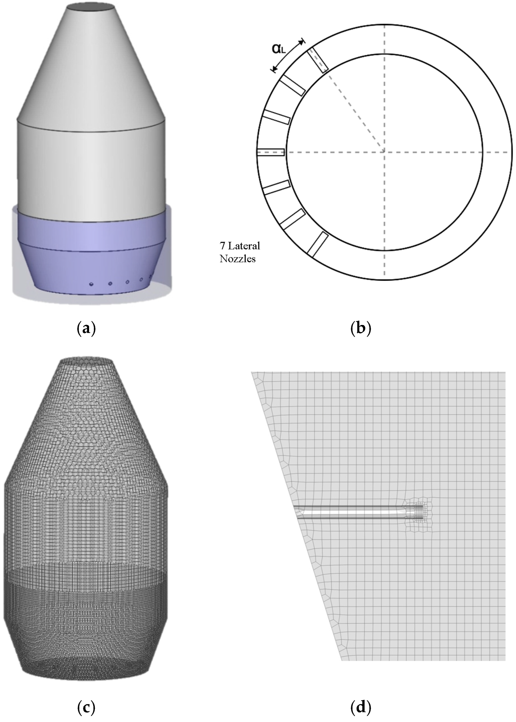
The simulated AOD converter in this work is shown in
Figure 1a; here, the seven lateral nozzles were placed in the conic inferior wall and the schematic upper view shown in
Figure 1b shows their disposal. It is an upper view where it can be appreciated that the nozzles are only on the left side; the purpose of this disposal is to avoid the gas fluxes in opposite directions that crash into each other. This fact hydro-dynamically supposes that these fluxes lose kinetic energy and turn back against the entering fluxes.
Figure 1c shows the meshing of the liquid volume for discretization.
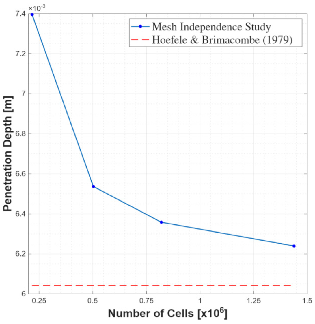
Figure 1d shows a meshing near the nozzle, evidencing that a fine mesh for discretization is required to obtain a good approach; this mesh employs 1.438 million nodes and it is a non-structured mesh with two adapted sizes, where the finest mesh is in the nozzles [
11,
12,
13,
14,
15,
16,
24,
25,
26,
27,
33,
34,
35,
36].
Inside the AOD converter, the melting steel is liquid and can be displaced by the intensity of the blowing gas which forms a horizontal penetration jet which when turned up forms a gas column additionally forming even bubbles or a constant column depending on the blowing conditions. The bubbles and columns are driven up due to its minor density; however, its contact allows for the displacement of a certain volume of the melting steel creating a turbulent fluid. During the AOD process, the gas behavior can be predicted using physical models or Computational Fluid Dynamics (CFD) [
11,
12,
13,
26,
27,
30,
31,
32,
33,
34,
39]. Additionally, the models can also employ the steel properties an air–water system for in laboratory experimentally controlled conditions, or, if the authors wish, can allow for the comparison of mathematical simulation results with a real physical model. The kinematic viscosity of steel at 1600 °C is 0.97 × 10
−6 m
2/s; in contrast, the water at 20 °C is 1 × 10
−6 m
2/s. Then, according to this similarity, a model based on Froude’s, Reynolds’s or Weber’s dimensionless numbers can be established for solving the simulation, and reliability is ensured [
11,
12,
13,
14,
15,
16,
30,
31,
32,
39].
Blowing is a typical industrial practice but frequently it is applied inefficiently due to unknown hydrodynamics; blowing inside an AOD converter is applied during decarburization to reduce the carbon content by chemical reaction with the oxygen in the gas column flowing out, consequently removing impurities. Then a high-carbon steel is converted into a low-carbon steel and then the other alloy elements can be added to produce different steel grades [
6,
7,
8,
9,
10,
26,
27,
33,
34].
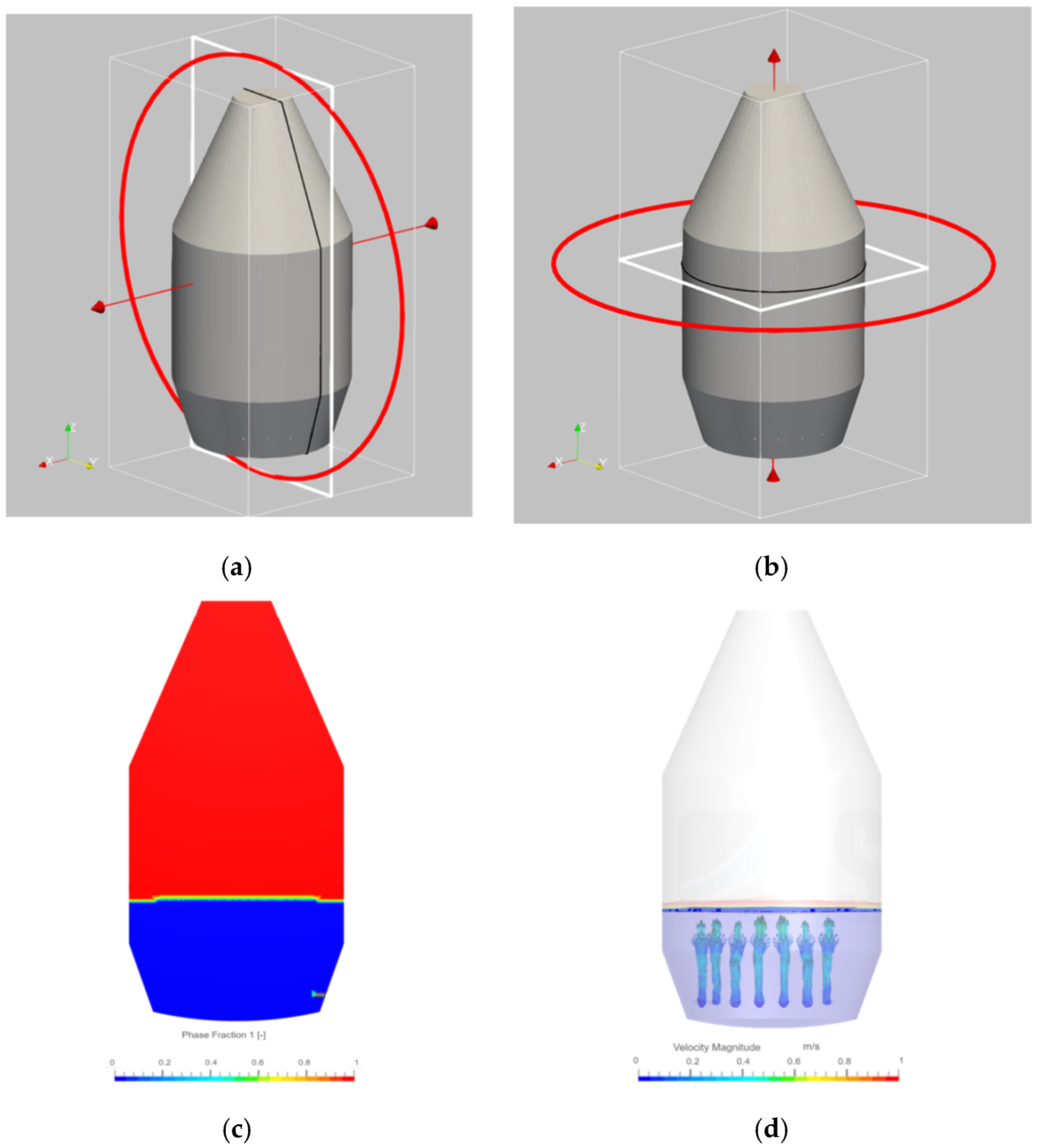
Figure 2a,b shows the cut planes where the hydrodynamical analysis is taken for calculation and comparison; the vertical plane in the middle location and the horizontal plane allow for the appreciation of the movement of the melting metal inside the bath and provide evidence of horizontal and vertical twirling formations. Considering two planes for analysis is helpful to understand 3D hydrodynamic behavior [
26,
27,
33,
34,
35,
43,
44,
45,
46,
47].
Additionally
Figure 2c,d shows the fractions inside the AOD converter for a time (t = 0) when the simulation is initially in a steady state and without movement.
Figure 2d shows the gas columns form when the argon and oxygen are blown and how these go up inside the melting bath [
1,
2,
3,
4,
11,
12,
13,
14,
18,
19,
20,
21,
43,
44,
45,
46,
47]. As in other pyro-metallurgical installations, walls of the converter are covered with refractory material to avoid thermal damage.
3. Assumptions for Numerical Simulation
The description of the math model is done by mentioning the assumptions and equations solved to show the hydrodynamical behavior of the melting steel. The following assumptions were taken into account for the simulated case.
- (a)
The simulation involves two fluids, the melting metal and the argon–oxygen gas mix; thus, the problem is assumed as two phases.
- (b)
Chemical activity between gas and the melting bath is not considered.
- (c)
It is assumed to be an isothermal process, and the melting bath is homogeneous; thus, the physical properties of the fluids remain constant.
- (d)
Water is used as the fluid to represent the liquid steel.
- (e)
No-slip condition in all AOD converter walls.
- (f)
Surface of the melting metal allows for waving. In consequence the meniscus level is the zone for the final dissipation of the kinetic energy applied to the melting metal.
- (g)
Maximum simulation time is ttotal = 50 s.
In this research only totally horizontal nozzles were simulated, but the possibility of a different angle of entry if the nozzles are angled towards the bottom or towards the upper-end of the melting bath can be considered.
The following equations were considered in the models for solving the discretized volume. Firstly, the Navier–Stokes Equations given by Claude-Louis Navier and George Gabriel Stokes represents the continuity of fluids. Equations (1) to (3) establish that divergence on the velocity field must be zero at every moment of the simulation.
Here u = u(x, t) is a vector field of the fluid in the position (x) at the time (t), p = p(x, t) is the pressure field at the same position and time, (v) is the kinematic viscosity,
is the gradient operator and
is the Lapalacian operator. Then, this equation can be written considering the density and the velocity of the fluids.
where (ρ) is the density of the fluid, (u) is the velocity vector, (p) is the pressure, (τ) is the tension tensor, (Cv) is the specific heat at constant volume and (Q) is the heat (T) is the temperature and (k) is the thermal conductivity; the equations of Navier–Stokes can be re-written as:
The turbulence models based on solving the Navier–Stokes equations and averaged by Reynolds are based on the evaluation of the effects of the turbulence fluctuations. The model m k-ϖ is used for considering the transport of adverse pressure gradients.
The model of volume of fluid (VOF) is used to simulate a system with two fluids: immiscible, considering an isothermal system, and uncompressible in a transitory state. Here a continuous velocity field between the interfaces is assumed, resulting in the following equation.
For a two-phase system with no miscible fluids, the continuity equation is modified resulting in Equations (7) and (8) respectively.
Here (U) is the velocity vector, (p) is the pressure of the fluid and (f
σ) is the surface force tension. (ρ) and (μ) are defined according to the fraction of the phase α as is shown in the equation:
The kinetic energy (KE) of the elements in a volume of fluid being stirred or in movement is a critical criterion to evaluate the efficiency of movement transferred. In a CFD simulation KE is calculated as a function of the velocity field at every time-step solving the equation.
As KE is an extensive quantity, it is necessary to solve the integral of the complete computational domino of the fluid to a continuous function, then
Thus, if (KE) is analyzed along with the time the progress of the transitory state can be evaluated and the maximum values remain stable or constant it is considered that a new steady state has been reached or the fluctuation of the kinetic energy and the turbulence have been minimized.
Although this was not considered, the explanation about the chemical reactions involved during decarburization are described in Equations (13) and (14).
Computational modeling involves the solution of the previous equations considered a no mass change during the simulation and the updating of the cells on the meshing with the percentages of the corresponding phase at every time-step (t + Δt).
5. Kinetic Energy Analysis
Decarburization is evaluated in the present work by considering the hydrodynamic behavior of the melting bath due to the chemical reaction between the gas blown and the melting metal. But the quantity of movement generated inside the melting bath can promote contact between gas and liquid molecules. The maximum simulation time is 50 s. This is considered to be a long enough time to consider the stability of forming twirling inside the bath. Then, it is assumed that for the rest of the time the hydrodynamics inside the bath variation is minimal.
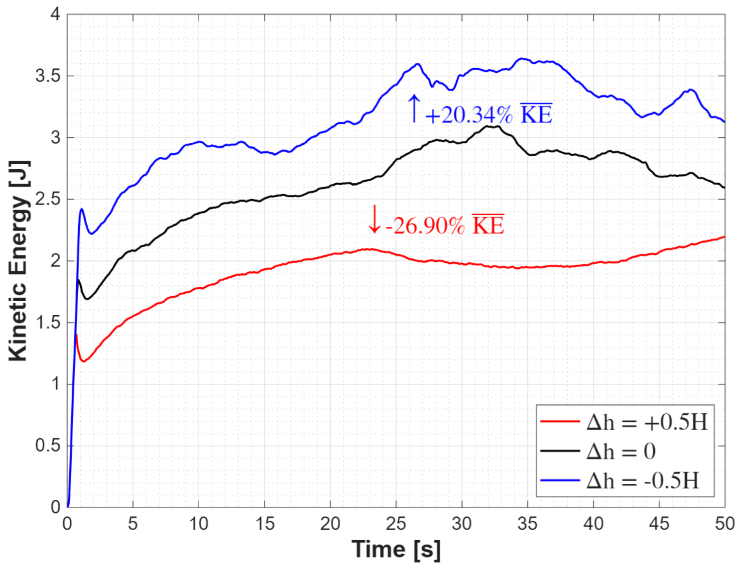
Kinetic energy (KE) was evaluated for the base case defined as (Δh = 0) but there are two more analyzed cases where (Δh = −0.5 H) and (Δh = +0.5 H) that evaluate the (KE) up and down the level where the nozzles were placed, as shown in
Figure 4. Here the fact that the major fluctuations are in the lower position due to the surface being near the gas-injected fluid can be appreciated; and the minor fluctuations are for the highest altitude of the melting steel.
The figure values of +20.34 and −26.90% result from the average between the measurements of kinetic energy for the cases +0.5 H and −0.5 H. The total fluctuations for the low volume in the AOD converter is slightly larger than for the upper volumes. Even if minor fluctuations in low volumes appreciate, kinetic energy and turbulence are also minor and consequently more predictable.
The analysis of the kinetic energy allows us to know the stability and un-stability of a fluid flow system.
Figure 4 shows the evaluation of the kinetic energy during the 50 s experiment testing three different altitudes inside the melting bath. The hydrodynamic analysis shows that at the beginning all curves began on the value for the kinetic energy (KE) = 0; because the steel is assumed as stationary and without movement, then the steel kinetic energy is immediately increased.
Here the curve above with the highest altitude (blue curve) also has the highest value due to the fact that in this position the fluid receives major kinetic energy. Values of this curve were taken at (Δh = −0.5 H), corresponding to the lowest altitude in the melting bath; here the kinetic energy has the highest values. After the initial simulation time, the three curves continue increasing their kinetic energy and having considerable fluctuations, but the fluctuation at the highest altitude also decreases; this means that the kinetic energy loses influence if it is so far from the application point. Due to the fact that a big heavy volume of fluid was displaced; before the 35 s experiment the fluctuation curves were reduced meaning that the motion of the melting steel tends to reduce fluctuation. In accordance with this, the kinetic energy changes as a function of the position inside the AOD converter where it is measured. The variation between the curves in this figure evidence that the dissipation of this energy is at the highest altitude at (Δh = +0.5 H) as demonstrated by the curve in the blue color, meaning the kinetic energy decreased as the analyzed fluid zone was far from the point where the blow (the nozzles) was applied. In addition, the curve in the red color has the lowest values of kinetic energy because a part of the kinetic energy has been already used to promote the movement of a certain volume of melting steel inside the bath. Nevertheless, as is shown in the figure, the kinetic energy also changes over time from an original stationary steady state, as the addition of an external force (argon and oxygen blowing) begins to displace the steel melting volume until the twirlings are completely formed and can be considered the final new stationary state. The curve in black presents an intermediate behavior with moderate fluctuations and less intense fluctuations.
The average distance between the curves evidence that the fluctuation of the kinetic energy and its consumption are due to the movement of a certain melting steel volume inside the bath. Perpendicular distances between these three curves are nearly the same for short times, but this distance is increased for simulation times between 30 and 40 s. Then the curves tend to reduce this variation, meaning sometimes the kinetic energy transmission and dissipation are different in accordance with the twirlings formed inside the bath. Additionally, the perpendicular distance between these curves means that a quantity of kinetic energy is used to displace the melting steel, while individual fluctuations mean certain instantaneous instability.
6. Hydrodynamic Analysis (Horizontal Profiles)
Figure 5,
Figure 6 and
Figure 7 show the results after the simulations. Here, the evolution of the fluid flow inside the melting bath considering a horizontal plane for analysis can be appreciated. A group of upper views are shown to illustrate the evolution of the fluid flow inside the bath.
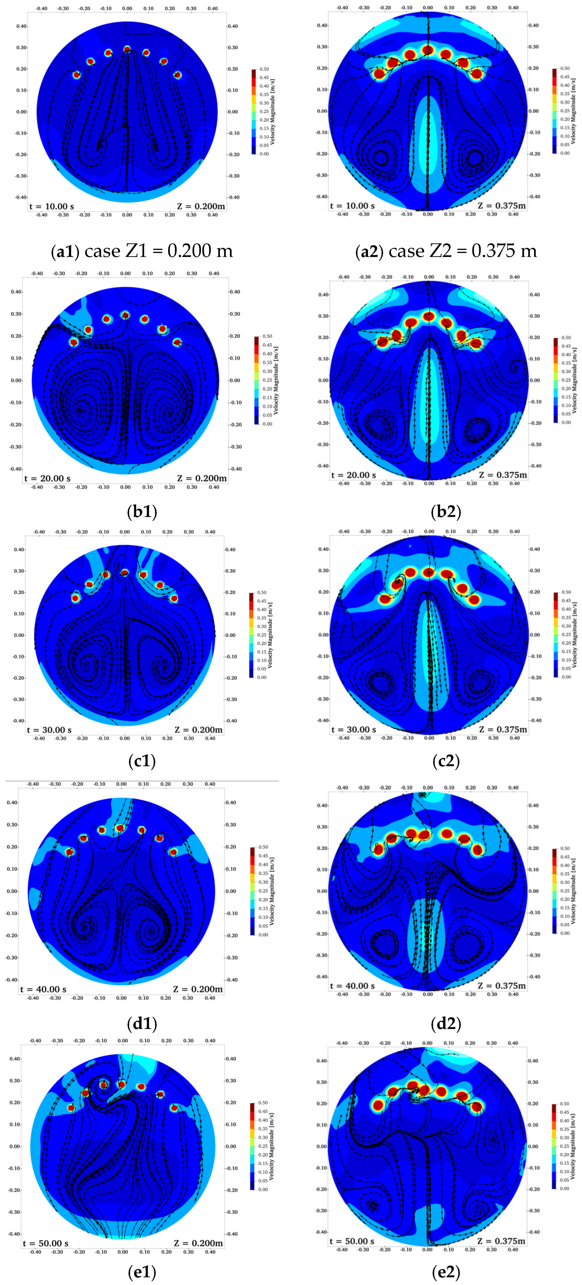
Figure 5 shows the basic case for different altitudes z1 = 0.200 and z2 = 0.375 m, considering the seven lateral nozzles case.
Figure 5 is divided to analyze two different altitudes inside the melting bath respectively; the hydrodynamic behavior studied at different simulation times and upper views were taken every 10 s. The analysis of the instability and hydrodynamic evolution can be appreciated in these figures.
Then, describing the basic case in
Figure 5, it is possible to describe the following hydrodynamic behaviors: In
Figure 5(a1) there are some points in the red color indicating the position of the nozzles placed, and consequently the highest velocity zones indicated in the red color appear; then, these are surrounded and push the fluid flow of melting steel towards the opposite AOD converter walls. The fluid crashed against the surrounding wall and in front the nozzles formed a quasi-symmetrical zone with a medium velocity, as indicated in the cyan color; the streamlines also indicate that the fluid was moved towards the opposite walls and some revolving behavior can be appreciated. Moreover, there are some streamlines behind the nozzles indicating that the fluid flow crashed against the AOD converter walls and turned back.
In
Figure 5(b1) here again the zones with high velocities are near the nozzles and here the zone of medium velocities in the opposite side of wall in the cyan color appear, but it is longer and more consolidated in comparison with the previous figure. Additionally, in this figure the streamlines indicate that the fluid flow forms big twirling zones which have certain influence over the melting steel movement.
In
Figure 5(c1) the nozzles continue with the highest velocity; but there are some areas of medium velocity surrounding them that appear. The other medium-velocity zone on the opposite side is early, constant and well formed. The streamline of the twirling looks more defined and some of the streamlines indicate that part of the fluid is sent back to near the nozzles to be re-circulated; in the middle zone of the AOD converter a zone of minimum speed remains.
Figure 5(d1) shows a 40 s measurement. Here, again the highest velocities are in the nozzles and surrounding them. In this figure some small zones near nozzles 1 and 7 and near the middle of the nozzles appear; the rest of the fluids in the middle of the AOD converter continue to have a very slow velocity. The streamlines indicate a pair of twirlings with a quasi-triangular external form being displaced towards the opposite wall side of the AOD converter. Moreover, these two twirlings tend to have a circular form in their centers and also have a few streamlines sent back towards the nozzles, again forming a re-circulating path.
Figure 5(e1) shows a 50 s measurement. Here in the middle of the AOD converter there is a low-velocity area and the middle velocity area which was formed in the opposite wall is the longest area and has been joined with the areas in the first and last nozzles. The streamlines indicate that twirlings have been pushed against the AOD converter walls, and a zone of instability has formed due to the twirlings’ crash.
Thus, for the basic case the gas is injected and the twirlings have an initiation stage; then a pair of twirling are formed quasi-symmetrically on the left and right sides for instance with a triangular perimetral form which tends to be circular in the central position. Then, these twirlings are pushed against the opposite walls of the AOD converter and finally collapse, crashing and re-driving the streamlines at the final simulation time (t = 50 s).
Now, analyzing the basic case for z2 = 0.375 it is possible to appreciate that in
Figure 5(a2) the highest velocities are again in the nozzle injection points; then, a quasi-symmetrical constant zone of the medium-velocity region on the walls near the nozzles can be appreciated. Additionally, quasi-symmetrical zones of medium velocity are formed beside the opposite side of the AOD converter wall. Moreover, in the middle of the AOD converter, other quasi-symmetrical regions with a medium velocity can be appreciated. The streamlines show quasi-symmetrical behavior with a pair of triangular twirlings with an elliptical center.
Figure 5(b2) shows some slightly bigger and deformed zones with a medium velocity surrounding the highest velocity areas where the influence of the gas blown by nozzles is appreciated. The areas on the opposite side of the AOD converter walls are increased and the areas of medium velocity behind the nozzles are separated. Streamlines show a triangular-centered twirling with an elliptical center being pushed against the lateral opposite sides, right and left, of the AOD converter walls.
In
Figure 5(c2), the same central area of medium velocity appears in the AOD converter; a big area of medium velocity surrounds the nozzles and triangular vortices become small with elliptical centers, but are pushed against the lateral sides of the AOD converter.
In
Figure 5(d2) the medium-velocity area surrounding the nozzles is almost a line and goes from side to side inside the AOD converter lateral walls. There are two isolated areas of medium velocity in the back wall near the central nozzles and are lightly displaced towards the opposite side of the AOD converter walls. The areas on the opposite sides became smaller. The streamlines show a pair of twirlings pushed against both sides of the AOD converter. The streamlines show a pair of defined triangular twirlings with a defined corridor in the central part of the AOD converter crashing into the opposite side of the AOD converter and being re-driven all around the AOD converter walls; and another path was formed when the twirling crashed into the streamlines pushed by the initial and latest nozzles, forming another pair of twirlings in the position near the first and latest nozzles.
In
Figure 5(e2) the twirling crashed and the streamlines disappeared. This is a collapse moment where only the gas columns blown by the nozzles can be appreciated and a small zone of medium velocity remains in the opposite side of the AOD converter walls.
After the previous description it is possible to affirm that there are many similarities between the profiles shown for the basic case, but the twirling morphologies and the velocity distributions also have certain particularities due to the altitude that they were taken. Moreover, it is so important to mention the following facts for the profiles shown:
- (a)
The percentage of colors indicate the total velocity generating movement in the analyzed surface of the AOD converter, which then can be related with the (KE) previous graphic in
Figure 4 indicating an overview about how this is being distributed and if it is being dissipated or conserved.
- (b)
The surfaces shown in
Figure 5 are taken at z1 = 0.200 m and 0.375 m from the AOD converter base surface; these are not aligned with the nozzle entries and consequently neither with the penetration of the gas jet. Consequently, for upper views it is not possible to appreciate the gas blown jets’ influence directly. The influence of the nozzles is circular or elliptical because we are watching the deformed form of the gas column flowing up.
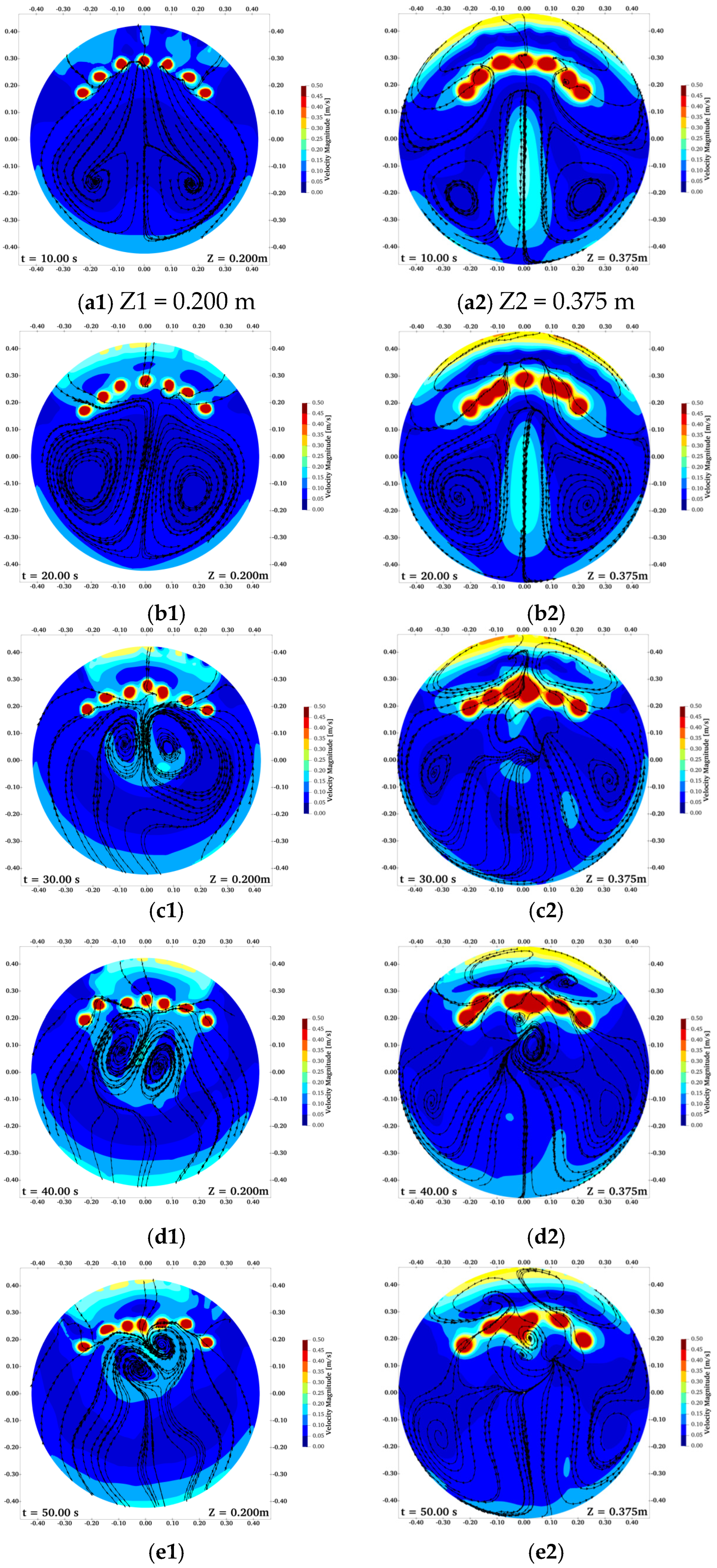
Figure 6 is shows the same altitudes, Z1 = 0.200 m. and z2 = 0.375 m., as
Figure 5 and were also analyzed for different simulation times considering the case h = −0.5 H. In
Figure 6(a1,a2) it is clear that the highest velocity zones are near the nozzles, but in
Figure 6(a2) there is a zone with medium velocity in the middle of the AOD converter. Moreover, there is a light but long area behind the nozzles (yellow zone), where the velocity is increased due to being crashed against the AOD converter walls. The zones of medium velocity appear in the opposite AOD converter walls; in both figures the streamlines let us see a pair of triangular twirlings but with particular differences. In
Figure 6(a1) the twirlings were formed from the fluid coming from an open driveway crash with the lateral walls, and then were re-driven towards the center; while in
Figure 6(a2) the twirlings were formed with the pushed flow.
Figure 6(b1,b2) are the corresponding figures for 20 s of simulation time. In
Figure 6(a1) there are some zones of medium velocity (cyan zone) surrounding the nozzles; there is another area quasi-symmetrically opposite to the AOD converter’s cylindrical wall. In the center there is a big area where velocity is so slow. The streamlines show a quasi-triangular pair of twirlings in the area of lowest velocities. In
Figure 6(b2) again there are two additional zones; the zone behind the nozzles with a high-velocity gradient is in yellow and the other is central, formed in the middle of the AOD converter.
Figure 6(c1,c2) are the corresponding figures for 30 s of simulation time. In
Figure 6(c1) the zone of medium velocity is nearly consolidated behind the nozzles. There is a zone of medium speed jumping out the center of the nozzles towards the middle of the AOD converter; the other zone on the opposite AOD converter wall has been increased and it is so thick. The twirling shows an elliptical morphology looking so defined and similar for the left and right sides, but in front of the twirlings there is a zone where the streamlines display a shocking behavior. In
Figure 6(c1), the zone with high-velocity (yellow zone) growth, the streamlines were dispersed along the cylindrical AOD converter walls behind the nozzles. There are a pair of isolated medium-velocity zones and two thin medium-velocity zones distributed along the opposite AOD converter wall. The streamlines form two isolated and small twirlings and in the middle of the AOD converter there are some poly-directional paths.
Figure 6(d1,d2) are the corresponding figures for 40 s of simulation time. Here the most notorious increase is the increase in the medium-velocity area on the opposite side of the AOD converter wall. Here, the middle of the zone with a slow velocity remains and the morphology of the area behind the nozzles is reduced but thicker; and there are two elliptical zones with a medium velocity just in front the seven nozzles. Here the streamlines in front of the seven nozzles form a pair of twirlings resulting from the backing fluid that crashed against the AOD converter opposite wall and which was re-driven against the original place from where it was moved. In contrast, in
Figure 6(d2) it is a bigger area of medium velocity in the opposite AOD converter wall and the area surrounding the central nozzles. Moreover, the yellow zone is now almost constant behind the nozzles; however, there is a zone of slow velocity between the yellow zone and the nozzles. The streamlines form a unique deviated twirling just in front of the central nozzles and the apparent quasi-formation of a pair of twirlings; but this is in angled position and not in the middle of the AOD converter.
Figure 6(e1,e2) are the corresponding figures for 50 s of simulation time. Here the zone of medium velocity in the opposite AOD converter walls continues growing alongside the area between the nozzles and behind the nozzles. With two areas of medium velocity that coincide with the direction of the streamlines indicating that the pair of twirlings have been formed near the nozzles, the fluid path in accordance with the streamlines was sent towards the AOD converter opposite walls and was sent back; even in
Figure 6(e2) a similar behavior can be appreciated.
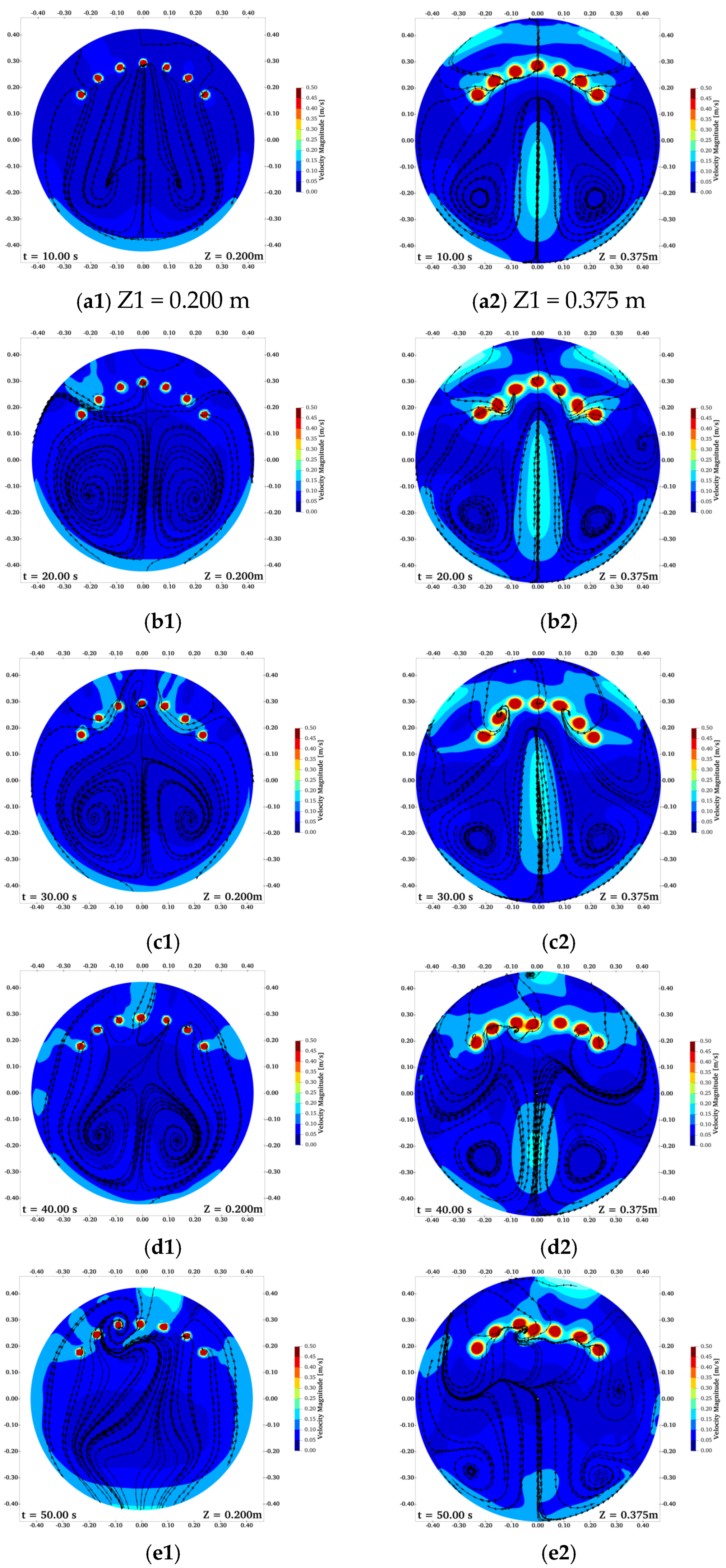
Figure 7 refers to the case h = +0.5 H; in
Figure 7 different altitudes are considered Z1 = 0.200 m and z2 = 0.375 m, as previously seen in
Figure 5 and
Figure 6. Again, these are analyzed to understand the hydrodynamic behavior of the steel bath inside the AOD converter. In
Figure 7(a1,a2) the injection of gas has begun. In
Figure 7(a1) only the nozzles appear as the zones with high velocity, and a zone on the opposite side of the AOD converter wall (cyan zone) has medium velocity; the rest of the AOD converter volume remains to have a very slow velocity. The streamlines are so straight because the fluids are just crashing in the middle zone of the AOD converter then streamlines are aligned towards the opposite wall and then the fluid is turned back to the zone near extreme side nozzles. In contrast,
Figure 7(a2) shows the central zone with a medium velocity in the middle of the AOD converter; there are two small zones on the AOD converter opposite wall, on the left and right sides. Moreover, a zone with a medium velocity is between the nozzles and the AOD converter back wall behind the nozzles. Here the streamlines form a quasi-symmetrical twirling from a triangular to a circular form in both sides of the AOD converter.
Figure 5,
Figure 6 and
Figure 7 show complimentary geometries for the velocity profiles inside the AOD converter. Then, the hydrodynamics at different altitudes evidence the re-driving of the fluid phenomena and the alignment of the streamlines. It is also appreciable that the maximum velocities are near the nozzles where the gas is blown. Moreover, the evolution of the fluid movement as a function of the simulation time can be followed. A zone of medium velocity is formed behind the nozzles; but zones with medium and slow velocities are in front of the nozzles due to the fact that there is a bigger steel volume to move.
Figure 5,
Figure 6 and
Figure 7 show almost a perfect symmetry for the horizontal profiles analyzed for the both left and right sides. Additionally, in accordance with the color scales in the profiles of
Figure 5,
Figure 6 and
Figure 7 the zones with high velocities are reduced and the influence of the gas columns to move the melting steel horizontally is limited.
Figure 7(c1,c2) represents 30 s of simulation time.
Figure 7(c1) looks so similar to the previous figure for 20 s of simulation time; but the streamlines seem to be inverted in comparison, and the quasi triangular twirling in the outside seems to be rotated.
Figure 7(c2) also looks similar to the previous figure, but the twirlings are more consolidated and were displaced towards the opposite AOD converter wall with a lightly lateral displacement.
Figure 7(d1) looks so similar to the previous figure with a big area in the middle zone of the AOD converter center, with the same tendency of the twirlings and only a few isolated zones with a medium velocity. In comparison
Figure 7(d2) is also similar to the previous figure but the zones in the middle of the AOD converter and surrounding the nozzles are bigger than in the previous figure. The streamlines form a central passage in the AOD converter and there are two quasi-symmetrical twirlings on the left and right sides. The back path makes a second pair of twirlings which are re-driven toward the nozzles and crash again being sent to the lateral walls.
Figure 7(e1,e2) are different because in both cases the twirlings were pushed towards the AOD converter wall excessively and then collapsed re-distributing the velocity profiles and the directions of the streamlines.
7. Hydrodynamic Analysis (Vertical Profiles)
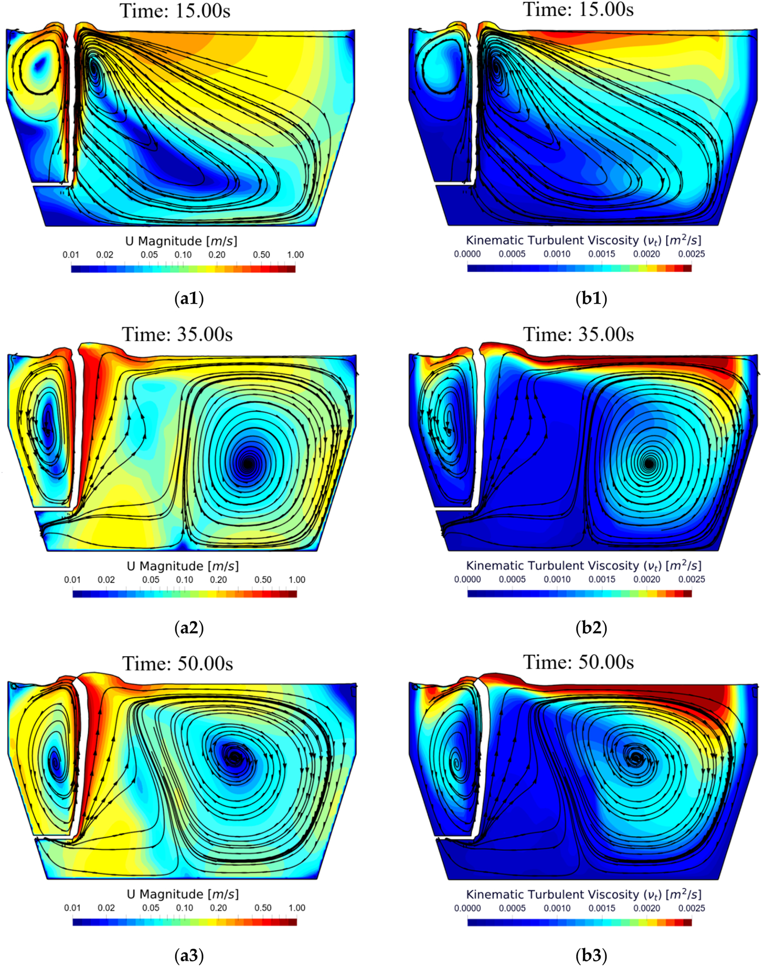
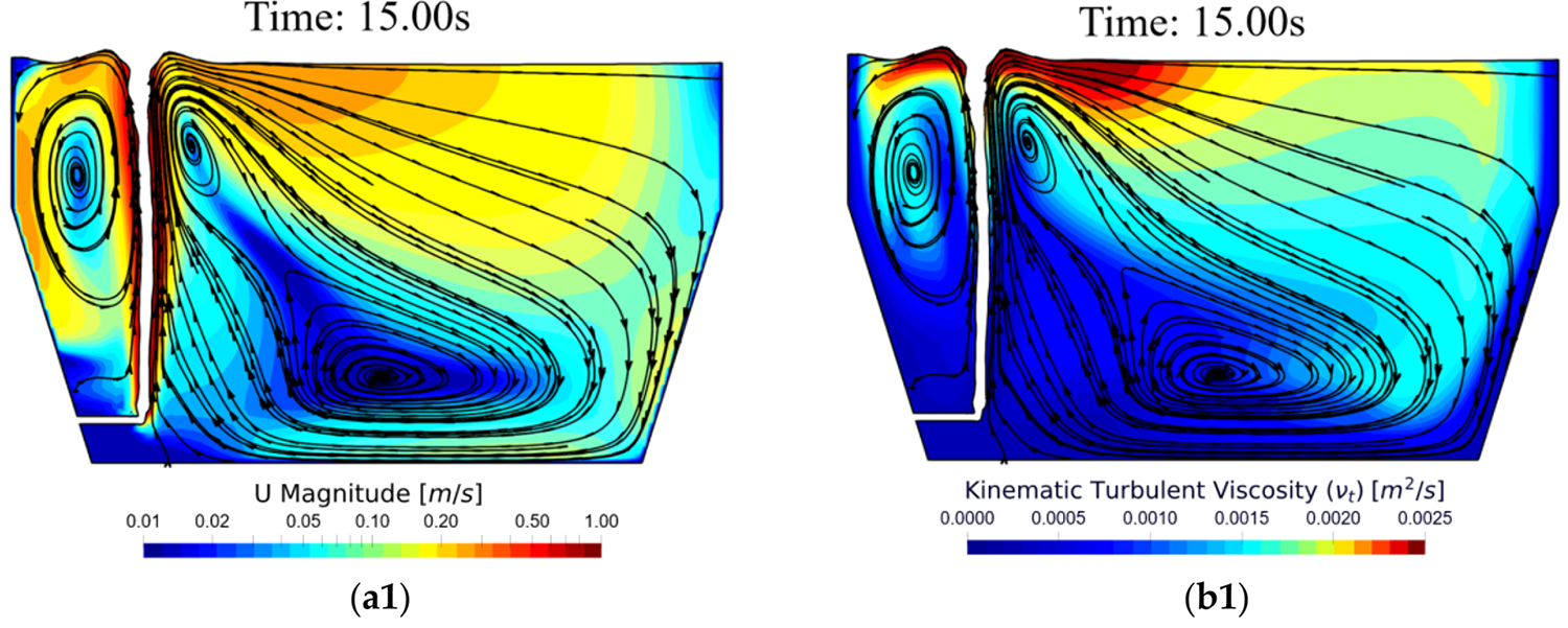
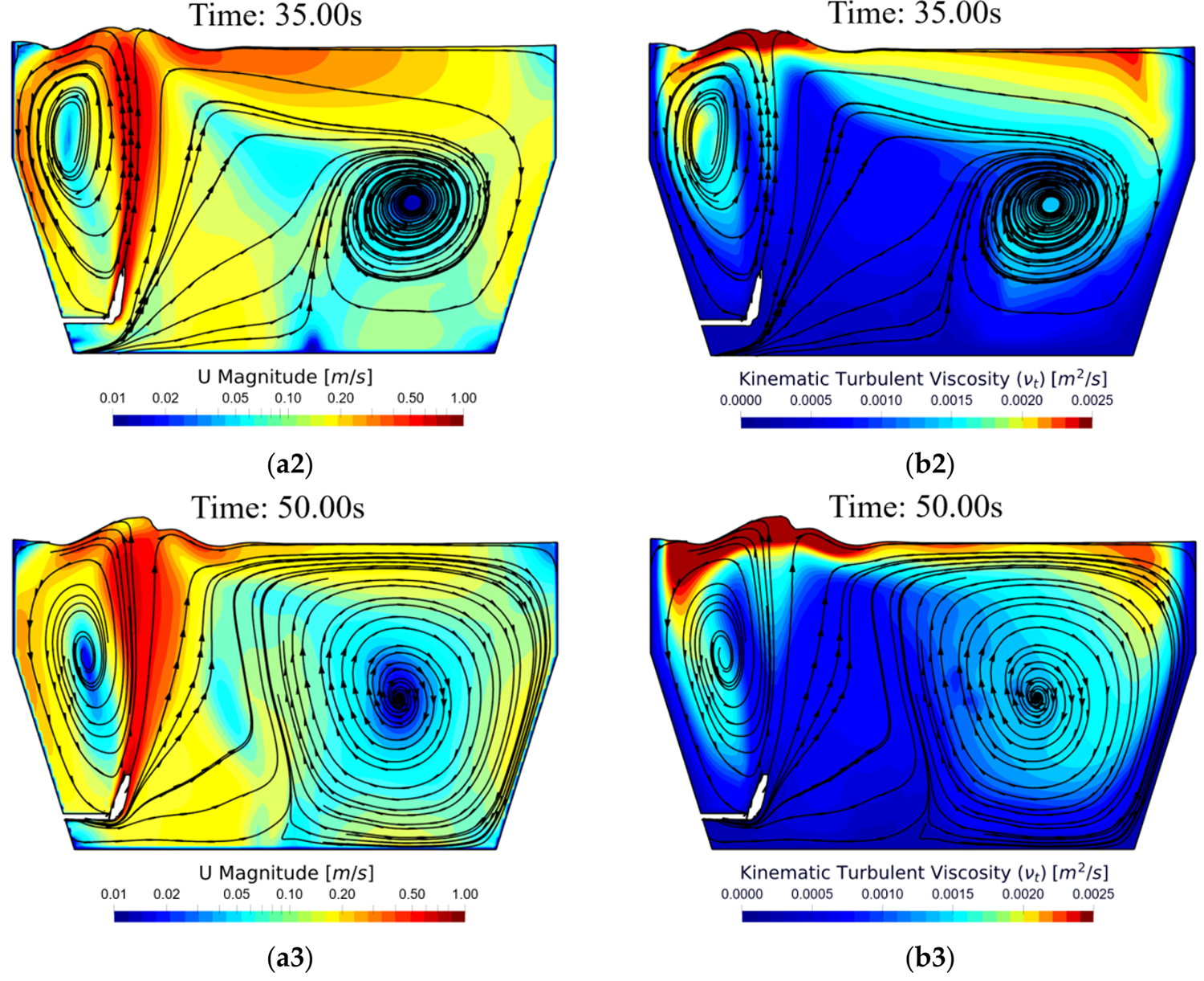
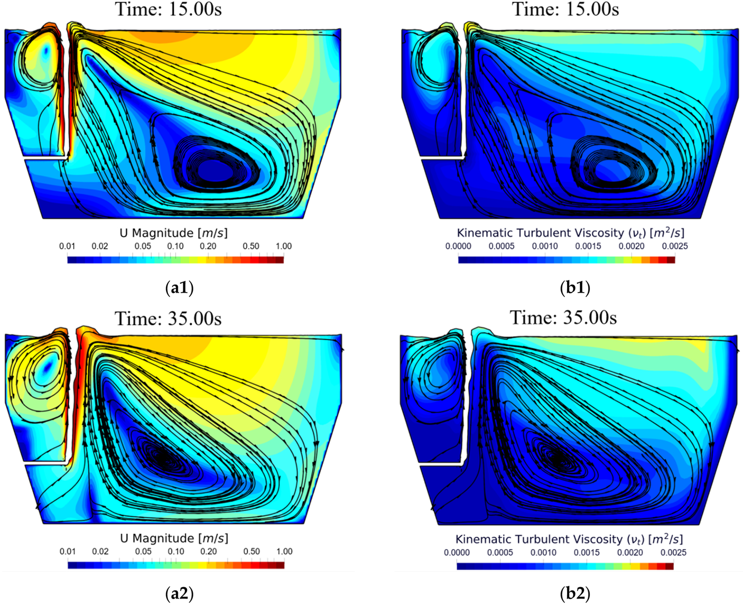
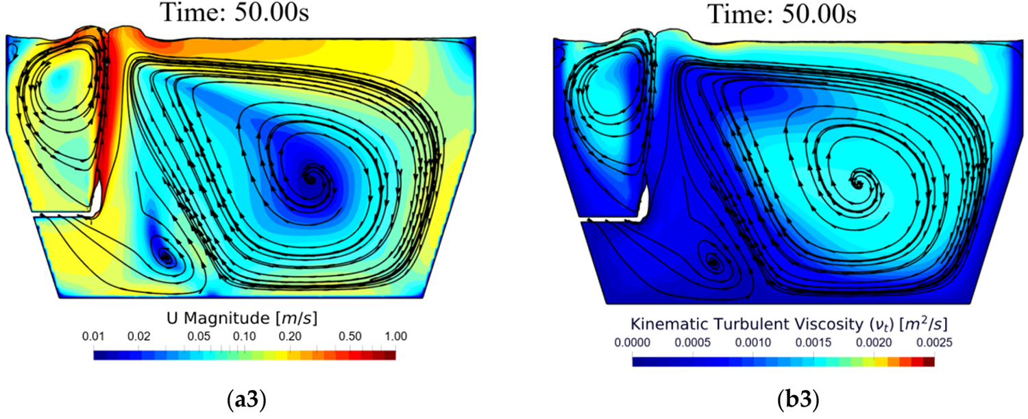
Figure 8,
Figure 9 and
Figure 10 show the velocity and the kinematic turbulent viscosity gradients and the streamline for the analyzed case in this work considering the vertical plane at the middle plane for the AOD converter. Thus,
Figure 8 is divided into two columns and the rows indicate the simulation time. Here the evolution of the twirlings can be appreciated.
Figure 8(a1) represents 15 s of simulation time. Then, the gas is blown inside the metallic bath and the jet penetrates a certain distance inside the melting steel bath, but promptly a gas column is formed indicating that the gas tends to go up towards the surface because the buoyancy forces begin to control its motion and its propulsion towards the surface. At this stage, the fluid, initially stationary, begins to be moved by the induced force of the gas blown from the nozzle. Here the streamlines result from displacement with a twirling pushed to the lower positions of the AOD converter. The gas going out of the melting steel’s surface tries to push the metal lower. Then, the twirling in the right side is deformed and pushed towards the opposite conical–cylindrical surface of the AOD converter and a secondary small twirling is formed behind the nozzle in the upper zone.
Figure 8(a2) shows the kinematic turbulent surface profiles; in this section the zones with major kinematic turbulent viscosity can be identified according to color. This is the case for the lowest and deepest zones of the AOD converter and near the nozzle. Here the streamlines are more similar than those in
Figure 8(a1).
Figure 8(b1,b2) correspond to 35 s. Here, there are more defined twirlings by the streamlines in the right side and also a defined quasi-elliptical small twirling in the left side (behind the gas column). In these figures the twirlings in the right side are also similar and a major jump displacement can be appreciated in the outlet surface area of the melting bath. The geometry of the twirling is almost defined; moreover, in both figures the twirlings formed with the streamlines have been pushed towards the opposite conic walls of the AOD converter. The twirling on the right side almost has a rectangular quasi-squared form in the perimeter and a circle in the middle altitude of the melting bath. Additionally, the twirling behind the nozzles is much more consolidated with a vertical elliptical form. Moreover, there is a stagnant zone in the middle of the AOD converter. The gas columns remain with a defined form showing a lightly deformed passage channel for leaking out.
In
Figure 8(c1,c2) the form of the twirlings are so consolidated and have been pushed to the opposite AOD converter walls for 50 s. of the simulation time; in both figures the twirlings on the right are lightly deformed due to some streamlines coming from the nozzle’s influence on the AOD converter. The twirling on the left side behind the nozzle gas jet is of a much more consolidate form; nevertheless the column is lightly deformed when the column of gas is near the bath’s surface. Here the gas column is curved and generates a waving movement when it arrives to the melting surface.
In all of
Figure 8, the highest velocity values are near the gas column appearing (red zone) in concordance with the perpendicular views shown in
Figure 5,
Figure 6 and
Figure 7. Another high-velocity zone is on the melting surface which indicates that the gas blown by nozzles is driven out and displaces the fluid creating a wave. The slower fluid displacements are in the deepest areas and the opposite side of the AOD converter. The zones in red promote the twirling formation but the zones in blue evidence that the mass of fluid is complicated to be displaced; in contrast the kinetic energy gradients show that the highest values are in the gas column but also in the surface of the melting bath. The column of gas is lightly deformed as a function of the dynamic buoyancy force and due to the hydrostatic pressure of the surrounding fluid; and it does not form a cylindrically defined or constant form. Moreover, there are zones in the twirling where velocity changes; then, there are zones where the fluid is accelerated or decelerated.
Figure 9 correspond to the analyzed case at (Δh = −0.5 H).
Figure 8 is divided into two columns, the first column shows the velocity gradient and the streamlines and the second column shows the kinematic viscosity; then,
Figure 9(a1,a2) show similar behaviors, the gradients of velocity and viscosity and the streamlines. In these figures, the twirling behind the gas column forms a small vertical quasi-elliptical. The twirling in the right side is also in formation. As the streamlines are sent to the depths and surface of the melting bath the twirling form is triangular in the right side; the gas column is nearly cylindrical. These profiles show the initial formation of the twirling. Thus, the morphology of the twirlings and velocity profiles change as simulation time goes on. During the initial 15 s of simulation time, the twirling on the right side was so deep inside the melting bath and there was a big stagnant zone on the upper side of the AOD converter wall opposite to the nozzles.
Figure 9(b1,b2) correspond to 35 s of simulation time. These figures also show a pair of unstable profiles. The twirling on the left side behind the gas column becomes elliptical but is deformed; the twirling on the right side is formed but remains so small. In comparison with the previous figures,
Figure 9(a1,a2), the streamlines have become a medium-size centered quasi-squared twirling in the perimeter, aligned with a quasi-circular twirling center.
These figures show the next step in the evolution of the twirlings on the left and right. But the gas column flowing up seems disappear due to sometimes being displaced because of the weight of the melting steel pushing against it. A high-velocity zone appeared in the gas path; thus, the gas was possibly compromised by the hydrostatic pressure of the metallic bath which formed a thin high-velocity gas column covered with a wall formed by the melting bath which was also pushed up and then displaced horizontally in accordance with the streamlines’ direction. But at the end the buoyancy force formed a bubble floating up.
Figure 9(c1,c2) show the consolidation of the twirlings. Here the twirling on the left side changes from an elliptical form to a little elliptical, and the twirling on the right side turns from a quasi-trapezoidal form in the perimeter to a vertical elliptical in the center of the melting bath. The twirlings in the right side have a medium velocity in the perimeter area but a slow velocity in the twirling center.
Figure 10 corresponds to the analyzed case at (Δh = +0.5 H). Here again there are two analyzed sub-cases in the columns; as can be appreciated for short times t = 10 s of the simulation time, the morphology of the twirlings in the left and right sides begin to be created and have a triangular form in concordance with the previous findings in
Figure 8 and
Figure 9. In the same way the figures for the times t = 15 s and 35 s are similar to those in the previous figures but show a delay in transformation because the undefined form in the twirling on the left side is evident and the triangular form in the right twirling also remains until 35 s. The profiles and streamlines for times 35 s and 50 s also have similarities; at the beginning of the simulation a triangular profile with a base in the deepest area of the AOD converter can be appreciated. Although, it changes into a squared twirling as the simulation time goes on; moreover, the right twirling influence is reduced near the bath surface in the opposite side of the AOD converter. The form of the twirling tends to be squared but in the center it is elliptical with a slow velocity and minimal streamlines.
The hydrodynamic behavior exposed in
Figure 8,
Figure 9 and
Figure 10 evidence the influence of the seven nozzles in pushing the melting steel over the velocity zones and the streamlines formed in the bath.
The profiles were taken over the analysis plane at different times showing some similarities and providing complimentary coherent information about the hydrodynamics inside the melting bath. In
Figure 8,
Figure 9 and
Figure 10 this can be appreciated again as the same hydrodynamic description is complimentary and shows similar behavior as was shown in
Figure 5,
Figure 6 and
Figure 7. Moreover, the information on vertical and horizontal analysis planes confirms the coherence of the calculus and can be used to build a 3D evolution of the twirling history.
9. Conclusions
In accordance with the velocities profiles and the kinetic energy analysis done, it is possible to conclude that kinetic energy is preferred for promoting the displacement of liquid metal inside the BOF with certain efficiency. Kinetic energy and turbulence are induced to the bath by the gas blown towards the BOF creating a pair of twirlings. One behind and one in front of the nozzles.
Decarburization only happens in the external face of the gas column because it is the only place where the carbon in the melting steel and the oxygen blown can be in contact; thus, hydrodynamic analysis is so important because it promotes steel movement and causes a chemical reaction with other components added to clean the steel.
The highest velocity zones are always near the nozzles who blow the gas, and this is the way to introduce kinetic energy to the stationary bath. Meanwhile medium-velocity zones are formed on the opposite side of the wall to the nozzle of the BOF and in the middle of the BOFs due to a convergence and alignment of the flux ejected by the central nozzles. As part of the hydrodynamic analysis, the kinetic energy produces a waving movement over the melting metal surface, becoming a zone in the dissipation energy area. Although the contact efficiency obtained from the hydrodynamic analysis calculated is promised, further analysis is necessary for a better understanding of the movements inside the melting bath. Some suggestions are listed below:
- (1)
Verifying the stability of system by measurement of kinetic energy and then plotting the hydrodynamic profiles using longer simulation times to understand the fluid flow movement entirely.
- (2)
Different steel casters: iron-making and steelmaking industries have different BOF configurations and dimensions; therefore, particular geometrical furnace configurations must be built and the corresponding simulations must be calculated for every one.
- (3)
Analyze the gas blown propulsion force or modify the nozzle length, angle or diameter to change the penetration depth of the gas as a part of a simulation with different geometrical configurations and parameter modifications because these are industrial variables that can be modified during real trials.
- (4)
Modify the angle disposed between the nozzles around the BOF body in order to assess more narrow or more spread out nozzle disposal. Include different volumes of melting steel in the same BOF which can cause different results in velocity and kinematic energy profiles.
- (5)
The influence of the gas blown out of the nozzles has a stronger influence over the vertical formation of twirling in contrast with the horizontal melting movement.
- (6)
After analyzing the horizontal and vertical profiles of the velocity and turbulence of kinetic energy it is possible to affirm that the gas column has a strong influence over the vertical movement of the fluid inside the AOD converter, but the influence is weak respectively to the horizontal movement. This is concluded analyzing color scales in both profiles.
- (7)
The vortexes are formed because the gas column injected inside the bath creates a displacement of the originally stationary melting steel; this movement causes melting when, at any point, it is in touch with the gas column. This increases the probability of a chemical reaction with the mix of argon and oxygen and the elimination of a certain volume of carbon. We promote this avenue for future research.
From the fluid mechanics point of view, the gas columns have a strong influence on vertical twirling; nevertheless, the twirling shown in the horizontal views is due to the influence of the lateral gas columns blown by the other seven nozzles surrounding the converter. Moreover, as these nozzles are distributed symmetrically, the horizontal twirlings are almost symmetrical.




 ,
,