Favard-Type Inequality on Symmetric Quantum Calculus

Abstract

In this paper, we establish a fundamental lemma based on symmetric quantum monotonicity within the framework of symmetric quantum calculus. Using this lemma, we derive the symmetric quantum Favard inequality and its Berwald-type extensions, together with generalizations to products of multiple functions and broader concavity classes. Numerical examples and comparative analyses demonstrate that the upper bounds obtained in the symmetric quantum framework are closer to the true integral values than those from the asymmetric quantum setting. This work establishes, for the first time, a complete theory of Favard–Berwald-type inequalities in symmetric quantum calculus, filling a gap in the literature and providing new analytical tools for quantum optimization and discrete integral estimation.

1. Introduction

The classical Favard inequality was first introduced by the French mathematician Jean Favard in 1933 [1]. It states that if $\psi \left(\theta \right)$ is a nonnegative concave function on $[a,b]$, then for any real number $p\ge 1$,

$$\frac{1}{b-a}{\int }_a^b{\psi }^p\left(\theta \right)\mathrm{d}\theta \le \frac{2^p}{p+1}{\left(\frac{1}{b-a}{\int }_a^b\psi \left(\theta \right)\mathrm{d}\theta \right)}^p.$$

(1)

This inequality provides a concise and powerful upper bound for the integral power of a concave function, with equality holding when $p=1$. Since its inception, the Favard inequality has attracted sustained research interest. In 1995, Maligranda et al. [2] established a more general weighted version, which further stimulated applications in approximation theory and physics, and led to the construction of Favard-type operators and related developments.

In recent years, quantum calculus [3], as a q-deformation of classical calculus, has demonstrated strong vitality in orthogonal polynomials, special functions, combinatorics, and approximation theory [4,5]. Within this framework, Yu [6] established in 2025 a q-Favard-type inequality in the asymmetric quantum setting:

$$\frac{1}{b-a}{\int }_a^b{\psi }^p\left(\theta \right){}_a\mathrm{d}_q\theta \le \frac{{\left[2\right]}_q^p}{{[p+1]}_q}{\left(\frac{1}{b-a}{\int }_a^b\psi \left(\theta \right){}_a\mathrm{d}_q\theta \right)}^p.$$

(2)

This result provided a new avenue for upper-bound estimation of quantum integrals and has potential applications in discrete energy estimation problems.

Meanwhile, fractional calculus, as a powerful tool for handling memory effects and nonlocal phenomena, has been widely applied in mathematical biology and epidemic modeling. Recently, Yunus et al. [7,8,9,10,11,12] systematically established fractional-order models for the transmission dynamics of several infectious diseases, employing Caputo fractional derivatives and the Laplace–Adomian decomposition method (LADM) to obtain analytical approximate solutions, and assessing the impact of vaccination, public awareness campaigns, and other intervention strategies on disease spread. These studies indicate that establishing refined integral inequalities within different calculus frameworks plays an important supporting role in the quantitative analysis of complex dynamical systems.

To obtain tighter upper bounds for integrals in the quantum setting than those available in the asymmetric case, Bilal et al. [13] and Vivas-Cortez et al. [14] introduced symmetric quantum calculus. This theory, by symmetrizing the q-derivative and q-integral, preserves the duality $q\leftrightarrow q^{-1}$, yielding inequalities that are not only more symmetric in form but also numerically sharper [15,16]. However, Favard-type inequalities in the symmetric quantum calculus framework have not been investigated previously.

In this paper, we establish, for the first time, Favard-type inequalities and their Berwald-type extensions within the symmetric quantum calculus framework. We first prove a fundamental lemma based on symmetric quantum monotonicity (Lemma 3), from which we derive the symmetric quantum Favard inequality (Theorem 3) and extend it to a broader class of functions for which ${\psi }^{1/\delta }$ is concave (Theorem 4). Furthermore, we obtain related inequalities for products of multiple functions (Theorems 5 and 6) and the symmetric quantum Berwald inequality (Theorems 7 and 8). Numerical examples and comparative analyses demonstrate that the upper bounds obtained in our symmetric framework are closer to the actual integral values than their asymmetric quantum counterparts, thereby validating the superiority of the symmetric approach. These results fill a gap in the theory of Favard-type inequalities in symmetric quantum calculus and provide new analytical tools for quantum optimization, discrete integral estimation, and related mathematical and physical problems.

2. Primary Knowledge

In symmetric quantum calculus, a fundamental concept is the symmetric quantum integer ${}_s\left[\alpha \right]_q$, which is defined in [4] as:

$${}_s\left[\alpha \right]_q=\frac{q^{-\alpha }-q^{\alpha }}{q^{-1}-q},\alpha \in \mathbb{R}.$$

(3)

Here, q is the quantum parameter, varying randomly within the interval $(0,1)$.

Definition 1

([8]). Let $\phi :I\to \mathbb{R}$ be a continuous mapping. For any $a,b\in I$ with $a<b$, the symmetric quantum derivative of the function φ at a point $\theta \in [a,b]$ is defined as:

$${}_{a}D_q^s\phi \left(\theta \right)=\frac{\phi (q^{-1}\theta +(1-q^{-1})a)-\phi (q\theta +(1-q)a)}{(q^{-1}-q)(\theta -a)},\theta \ne a.$$

(4)

At $\theta =a$, we define ${}_{a}D_q^s\phi \left(a\right)={\displaystyle \underset{\theta \to a^{+}}{lim}}{}_{a}D_q^s\phi \left(\theta \right)$. If $a=0$, the above symmetric quantum derivative reduces to the Jackson-type symmetric quantum derivative (see [4]).

In Definition 1, since $q\in (0,1)$, for any $\theta \in [a,b]\subset I$, it is straightforward to obtain:

$$q^{-1}\theta +(1-q^{-1})a-[q\theta +(1-q)a]=(q^{-1}-q)(\theta -a)\ge 0.$$

(5)

Hence,

$$q^{-1}\theta +(1-q^{-1})a\ge q\theta +(1-q)a.$$

(6)

Therefore, if ${}_{a}D_q^s\phi \left(\theta \right)\ge 0$, the function $\phi \left(\theta \right)$ is said to be symmetric quantum monotone increasing on the interval I; otherwise, it is called symmetric quantum monotone decreasing. In fact, if a function $\phi \left(\theta \right)$ is classically monotone increasing on I, then it is necessarily symmetric quantum monotone increasing on I. This property is crucial for establishing the Favard inequality on symmetric quantum integrals in Section 3 of this paper.

If both $\phi$ and $\varphi$ are symmetric quantum differentiable on I, then for any $[a,b]\subset I$ and any real numbers ${\mu }_1,{\mu }_2$, the symmetric quantum derivative satisfies the following operational rules:

Theorem 1

([8]). Let $\phi ,\varphi :I\to \mathbb{R}$ be continuous mappings. Then for any $[a,b]\subset I$ and any real numbers ${\mu }_1,{\mu }_2$, we have:

$$\begin{array}{cc}\hfill & \left(1\right){}_{a}D_q^s[{\mu }_1\phi \left(\theta \right)+{\mu }_2\varphi \left(\theta \right)]={\mu }_1{}_{a}D_q^s\phi \left(\theta \right)+{\mu }_2{}_{a}D_q^s\varphi \left(\theta \right);\hfill \\ \hfill & \left(2\right){}_{a}D_q^s[\phi \left(\theta \right)·\varphi \left(\theta \right)]=\phi (q^{-1}\theta +(1-q^{-1})a){}_{a}D_q^s\varphi \left(\theta \right)+\varphi (q\theta +(1-q)a){}_{a}D_q^s\phi \left(\theta \right);\hfill \\ \hfill & \left(3\right){}_{a}D_q^s\frac{\phi \left(\theta \right)}{\varphi \left(\theta \right)}=\frac{\varphi (q\theta +(1-q)a){}_{a}D_q^s\phi \left(\theta \right)-\phi (q\theta +(1-q)a){}_{a}D_q^s\varphi \left(\theta \right)}{\varphi (q\theta +(1-q)a)\varphi (q^{-1}\theta +(1-q^{-1})a)},\varphi \left(\theta \right)\ne 0.\hfill \end{array}$$

If ${}_{a}D_q^s{\rm Y}\left(\theta \right)=\phi \left(\theta \right)$ for $\theta \in [a,b]$, then the function ${\rm Y}\left(\theta \right)$ is called a symmetric quantum antiderivative (or primitive) of $\phi \left(\theta \right)$ on $[a,b]$. From the definition of the symmetric quantum derivative, it is easy to verify that:

$$\begin{array}{cc}\hfill {}_{a}D_q^s{(\theta -a)}^{\alpha +1}& =\frac{{(q^{-1}\theta +(1-q^{-1})a-a)}^{\alpha +1}-{(q\theta +(1-q)a-a)}^{\alpha +1}}{(q^{-1}-q)(\theta -a)}\hfill \\ \hfill & ={}_s[\alpha +1]_q{(\theta -a)}^{\alpha }.\hfill \end{array}$$

Consequently, the function ${\rm Y}\left(\theta \right)=\frac{1}{{}_s[\alpha +1]_q}{(\theta -a)}^{\alpha +1}$ is a symmetric quantum antiderivative of the function $\phi \left(\theta \right)={(\theta -a)}^{\alpha }$ on [a, b], where $\alpha \ne -1$.

Definition 2

([8]). Let $\phi :I\to \mathbb{R}$ be a continuous mapping. For any $a,b\in I$ with $a<b$, the symmetric quantum integral of the function φ over the interval $[a,b]\subset I$ is defined as:

$${\int }_a^b\phi \left(\theta \right){}_{a}d_q^s\theta =(b-a)(1-q^2){\displaystyle \sum _{n=0}^{\infty }}{q}^{2n}\phi (q^{2n+1}b+(1-q^{2n+1})a).$$

(7)

If the series ${\displaystyle \sum _{n=0}^{\infty }}{q}^{2n}\phi (q^{2n+1}b+(1-q^{2n+1})a)$ converges, then φ is said to be symmetric quantum integrable on I.

For continuous functions $\phi \left(t\right)$ and $\varphi \left(t\right)$, if $\phi \left(t\right)\ge \varphi \left(t\right)$ holds for all $t\in I$, then for each n we have:

$$(t-a)(1-q^2)\phi (q^{2n+1}t+(1-q^{2n+1})a)\ge (t-a)(1-q^2)\varphi (q^{2n+1}t+(1-q^{2n+1})a).$$

(8)

Summing the above inequalities yields:

$${\int }_a^t\phi \left(\theta \right){}_a\mathrm{d}_q^s\theta \ge {\int }_a^t\varphi \left(\theta \right){}_a\mathrm{d}_q^s\theta ,$$

(9)

which shows that the symmetric quantum integral satisfies the order-preserving property.

From the definition of the symmetric quantum integral, the following change-of-variable formulas are readily derived:

$$\begin{array}{cc}\hfill {\int }_a^{qb+(1-q)a}\phi \left(\theta \right){}_a\mathrm{d}_q^s\theta & =q(b-a)(1-q^2){\displaystyle \sum _{n=0}^{\infty }}{q}^{2n}\phi (q^{2n+2}b+q^{2n+1}(1-q)a+(1-q^{2n+1})a)\hfill \\ \hfill & =q(b-a)(1-q^2){\displaystyle \sum _{n=0}^{\infty }}{q}^{2n}\phi (q^{2n+2}b-q^{2n+2}a+a)\hfill \\ \hfill & =q(b-a)(1-q^2){\displaystyle \sum _{n=0}^{\infty }}{q}^{2n}\phi (q(q^{2n+1}b+(1-q^{2n+1})a)+(1-q)a)\hfill \\ \hfill & =q{\int }_a^b\phi (q\theta +(1-q)a){}_a\mathrm{d}_q^s\theta .\hfill \end{array}$$

Similarly, we obtain:

$${\int }_a^{q^{-1}b+(1-q^{-1})a}\phi \left(\theta \right){}_a\mathrm{d}_q^s\theta =q^{-1}{\int }_a^b\phi (q^{-1}\theta +(1-q^{-1})a){}_a\mathrm{d}_q^s\theta .$$

Thus, we have the following lemma:

Lemma 1.

Let $\phi ,\varphi :I\to \mathbb{R}$ be continuous mappings. Then for any $[a,b]\subset I$, we have:

$$\begin{array}{cc}\hfill & \left(1\right){\int }_a^{qb+(1-q)a}\phi \left(\theta \right){}_{a}d_q^s\theta =q{\int }_a^b\phi (q\theta +(1-q)a){}_{a}d_q^s\theta ;\hfill \\ \hfill & \left(2\right){\int }_a^{q^{-1}b+(1-q^{-1})a}\phi \left(\theta \right){}_{a}d_q^s\theta =q^{-1}{\int }_a^b\phi (q^{-1}\theta +(1-q^{-1})a){}_{a}d_q^s\theta .\hfill \end{array}$$

The symmetric quantum integral obeys the following operational rules:

Theorem 2

([9]). Let $\phi ,\varphi :I\to \mathbb{R}$ be continuous mappings. Then for any $t\in [a,b]\subset I$ and any real numbers ${\mu }_1,{\mu }_2$, we have:

$$\begin{array}{cc}\hfill & \left(1\right){\int }_a^b[{\mu }_1\phi \left(\theta \right)+{\mu }_2\varphi \left(\theta \right)]{}_{a}d_q^s\theta ={\mu }_1{\int }_a^b\phi \left(\theta \right){}_{a}d_q^s\theta +{\mu }_2{\int }_a^b\varphi \left(\theta \right){}_{a}d_q^s\theta ;\hfill \\ \hfill & \left(2\right){\int }_a^t{}_{a}D_q^s\phi \left(\theta \right){}_{a}d_q^s\theta ={\left.\phi \left(\theta \right)\right|}_a^t=\phi \left(t\right)-\phi \left(a\right);\hfill \\ \hfill & \left(3\right){}_{a}D_q^s{\int }_a^t\phi \left(\theta \right){}_{a}d_q^s\theta =\phi \left(t\right);\hfill \\ \hfill & \left(4\right){\int }_a^b\phi (q^{-1}\theta +(1-q^{-1})a){}_{a}D_q^s\varphi \left(\theta \right){}_{a}d_q^s\theta ={\left.\phi \left(\theta \right)\varphi \left(\theta \right)\right|}_a^b-{\int }_a^b\varphi (q\theta +(1-q)a){}_{a}D_q^s\phi \left(\theta \right){}_{a}d_q^s\theta .\hfill \end{array}$$

In Theorem 2, Formula (4) is called the integration by parts formula for the symmetric quantum integral. It is obtained by applying the symmetric quantum integral to both sides of Formula (2) in Theorem 1. Similarly, we can also derive:

$${\int }_a^b\varphi (q\theta +(1-q)a){}_{a}D_q^s\phi \left(\theta \right){}_a\mathrm{d}_q^s\theta ={\left.\phi \left(\theta \right)\varphi \left(\theta \right)\right|}_a^b-{\int }_a^b\phi (q^{-1}\theta +(1-q^{-1})a){}_{a}D_q^s\varphi \left(\theta \right){}_a\mathrm{d}_q^s\theta .$$

Clearly, since ${\rm Y}\left(\theta \right)=\frac{1}{{}_s[\alpha +1]_q}{(\theta -a)}^{\alpha +1}$ is a symmetric quantum antiderivative of $\phi \left(\theta \right)={(\theta -a)}^{\alpha }$ on the interval $[a,b]$ (where $\alpha \ne -1$), it follows that:

$${\int }_a^b{(\theta -a)}^{\alpha }{}_a\mathrm{d}_q^s\theta ={\left.\frac{1}{{}_s[\alpha +1]_q}{(\theta -a)}^{\alpha +1}\right|}_a^b=\frac{{(b-a)}^{\alpha +1}}{{}_s[\alpha +1]_q}.$$

(10)

From Formula (3) in Theorem 1, we obtain the following lemma:

Lemma 2.

Let $\varphi :I\to \mathbb{R}$ be a continuous positive mapping, and let $\phi \left(t\right)=k{(t-a)}^{\alpha }$, where $k\in \mathbb{R}$ and $\alpha >0$. Then for every $t\in (a,b]\subset I$, the function

$$\mathsf{\Psi }\left(t\right)=\frac{{\int }_a^t\phi \left(\theta \right)\varphi \left(\theta \right){}_{a}d_q^s\theta }{{\int }_a^t\phi \left(\theta \right){}_{a}d_q^s\theta }.$$

(11)

has the same monotonicity as $\varphi \left(t\right)$ on $(a,b]$.

Proof. 

Take arbitrary $t_1,t_2\in (a,b]$ with $t_1<t_2$. Then,

$$\begin{array}{cc}\hfill \mathsf{\Psi }\left(t_2\right)-\mathsf{\Psi }\left(t_1\right)& =\frac{{\int }_a^{t_2}\phi \left(\theta \right)\varphi \left(\theta \right){}_a\mathrm{d}_q^s\theta }{{\int }_a^{t_2}\phi \left(\theta \right){}_a\mathrm{d}_q^s\theta }-\frac{{\int }_a^{t_1}\phi \left(\theta \right)\varphi \left(\theta \right){}_a\mathrm{d}_q^s\theta }{{\int }_a^{t_1}\phi \left(\theta \right){}_a\mathrm{d}_q^s\theta }\hfill \\ \hfill & =\frac{{\int }_a^{t_1}\phi \left(\theta \right){}_a\mathrm{d}_q^s\theta ·{\int }_a^{t_2}\phi \left(\theta \right)\varphi \left(\theta \right){}_a\mathrm{d}_q^s\theta -{\int }_a^{t_2}\phi \left(\theta \right){}_a\mathrm{d}_q^s\theta ·{\int }_a^{t_1}\phi \left(\theta \right)\varphi \left(\theta \right){}_a\mathrm{d}_q^s\theta }{{\int }_a^{t_1}\phi \left(\theta \right){}_a\mathrm{d}_q^s\theta ·{\int }_a^{t_2}\phi \left(\theta \right){}_a\mathrm{d}_q^s\theta }\hfill \\ \hfill & =\frac{\frac{{(t_1 - a)}^{\alpha +1}}{{}_s[\alpha +1]_q}·{\int }_a^{t_2}{(\theta -a)}^{\alpha }\varphi \left(\theta \right){}_a\mathrm{d}_q^s\theta -\frac{{(t_2 - a)}^{\alpha +1}}{{}_s[\alpha +1]_q}·{\int }_a^{t_1}{(\theta -a)}^{\alpha }\varphi \left(\theta \right){}_a\mathrm{d}_q^s\theta }{\frac{{(t_1 - a)}^{\alpha +1}}{{}_s[\alpha +1]_q}·\frac{{(t_2 - a)}^{\alpha +1}}{{}_s[\alpha +1]_q}}\hfill \\ \hfill & =\frac{{(t_1-a)}^{\alpha +1}·{\int }_a^{t_2}{(\theta -a)}^{\alpha }\varphi \left(\theta \right){}_a\mathrm{d}_q^s\theta -{(t_2-a)}^{\alpha +1}·{\int }_a^{t_1}{(\theta -a)}^{\alpha }\varphi \left(\theta \right){}_a\mathrm{d}_q^s\theta }{{(t_1-a)}^{\alpha +1}·{(t_2-a)}^{\alpha +1}}\hfill \\ \hfill & ·{}_s[\alpha +1]_q.\hfill \end{array}$$

Now consider the numerator difference:

$$\begin{array}{cc}\hfill & {(t_1-a)}^{\alpha +1}·{\int }_a^{t_2}{(\theta -a)}^{\alpha }\varphi \left(\theta \right){}_a\mathrm{d}_q^s\theta -{(t_2-a)}^{\alpha +1}·{\int }_a^{t_1}{(\theta -a)}^{\alpha }\varphi \left(\theta \right){}_a\mathrm{d}_q^s\theta \hfill \\ \hfill & ={(t_1-a)}^{\alpha +1}·(t_2-a)(q^{-1}-q){\displaystyle \sum _{n=0}^{\infty }}{q}^{2n+1}{(q^{2n+1}{t}_2-q^{2n+1}a)}^{\alpha }\varphi (q^{2n+1}{t}_2+(1-q^{2n+1})a)\hfill \\ \hfill & -{(t_2-a)}^{\alpha +1}·(t_1-a)(q^{-1}-q){\displaystyle \sum _{n=0}^{\infty }}{q}^{2n+1}{(q^{2n+1}{t}_1-q^{2n+1}a)}^{\alpha }\varphi (q^{2n+1}{t}_1+(1-q^{2n+1})a)\hfill \\ \hfill & ={(t_1-a)}^{\alpha +1}·{(t_2-a)}^{\alpha +1}(q^{-1}-q)·\hfill \\ \hfill & {\displaystyle \sum _{n=0}^{\infty }}{q}^{2n+1}{\left(q^{2n+1}\right)}^{\alpha }[\varphi (q^{2n+1}{t}_2+(1-q^{2n+1})a)-\varphi (q^{2n+1}{t}_1+(1-q^{2n+1})a)].\hfill \end{array}$$

Since $\phi \left(t\right)>0$, the sign of ${}_{a}D_q^s\mathsf{\Psi }\left(t\right)$ is determined by $\varphi \left(t\right)-\varphi \left(\theta \right)$. Noting that

$$a\le \theta \le qt+(1-q)a\le t,$$

(12)

we conclude that if $\varphi \left(t\right)$ is symmetric quantum monotone increasing, then $\varphi \left(t\right)-\varphi \left(\theta \right)\ge 0$ and consequently ${}_{a}D_q^s\mathsf{\Psi }\left(t\right)\ge 0$. This implies that $\mathsf{\Psi }\left(t\right)$ is also symmetric quantum increasing on $(a,b]$. If $\varphi \left(t\right)$ is symmetric quantum monotone decreasing, then ${}_{a}D_q^s\mathsf{\Psi }\left(t\right)\le 0$, and thus, the function $\mathsf{\Psi }\left(t\right)$ is symmetric quantum decreasing on $(a,b]$. This completes the proof of Lemma 2. □

3. Main Results

Lemma 3.

Let $\phi ,\varphi :I\to \mathbb{R}$ be nonnegative mappings, and both are symmetric quantum integrable. If they satisfy:

$$\begin{array}{cc}\hfill & \left(i\right){\int }_a^{qt+(1-q)a}\phi \left(\theta \right){}_{a}d_q^s\theta \le {\int }_a^{qt+(1-q)a}\varphi \left(\theta \right){}_{a}d_q^s\theta ,t\in [a,b);\hfill \\ \hfill & \left(ii\right){\int }_a^{qb+(1-q)a}\phi \left(\theta \right){}_{a}d_q^s\theta ={\int }_a^{qb+(1-q)a}\varphi \left(\theta \right){}_{a}d_q^s\theta .\hfill \end{array}$$

Then for any constant $p\ge 1$, we have:

(1) When φ is monotone decreasing on $[a,b]$:

$${\int }_a^{qb+(1-q)a}{\phi }^p\left(\theta \right){}_{a}d_q^s\theta \le {\int }_a^{qb+(1-q)a}{\varphi }^p\left(\theta \right){}_{a}d_q^s\theta ;$$

(13)

(2) When ϕ is monotone increasing on $[a,b]$:

$${\int }_a^{qb+(1-q)a}{\varphi }^p\left(\theta \right){}_{a}d_q^s\theta \le {\int }_a^{qb+(1-q)a}{\phi }^p\left(\theta \right){}_{a}d_q^s\theta .$$

(14)

Proof. 

Consider the function $\delta \left(t\right)=t^p$. Since $p\ge 1$, $\delta \left(t\right)$ is convex on the interval I. Therefore, for any ${\omega }_1,{\omega }_2\in I$, and ${\omega }_1,{\omega }_2>0$.

$${\omega }_1^p-{\omega }_2^p\le p{\omega }_1^{p-1}({\omega }_1-{\omega }_2),$$

(15)

it follows that

$$\begin{array}{cc}\hfill & {\phi }^p(qt+(1-q)a)-{\varphi }^p(qt+(1-q)a)\hfill \\ \hfill & \le p{\phi }^{p-1}(qt+(1-q)a)[\phi (qt+(1-q)a)-\varphi (qt+(1-q)a)].\hfill \end{array}$$

(16)

Construct an auxiliary function:

$$\begin{array}{cc}\hfill {\rm Y}\left(t\right)& ={\int }_a^{qt+(1-q)a}[\phi \left(\theta \right)-\varphi \left(\theta \right)]{}_a\mathrm{d}_q^s\theta \hfill \\ \hfill & =q{\int }_a^t[\phi (q\theta +(1-q)a)-\varphi (q\theta +(1-q)a)]{}_a\mathrm{d}_q^s\theta \hfill \end{array}$$

(17)

Then on the interval $[a,b)$, we have ${\rm Y}\left(t\right)\le 0$, and ${\rm Y}\left(a\right)={\rm Y}\left(b\right)=0$. Also,

$${}_{a}D_q^s{\rm Y}\left(t\right)=q[\phi (qt+(1-q)a)-\varphi (qt+(1-q)a)].$$

(18)

(1) When $\phi \left(t\right)$ is monotonically decreasing, by the integration by parts for symmetric quantum integrals (Formula (4) of Theorem 2),

$$\begin{array}{cc}\hfill & {\int }_a^{qb+(1-q)a}[{\phi }^p\left(\theta \right)-{\varphi }^p\left(\theta \right)]{}_a\mathrm{d}_q^s\theta \hfill \\ \hfill & =q{\int }_a^b[{\phi }^p(q\theta +(1-q)a)-{\varphi }^p(q\theta +(1-q)a)]{}_a\mathrm{d}_q^s\theta \hfill \\ \hfill & \le pq{\int }_a^b{\phi }^{p-1}(q\theta +(1-q)a)[\phi (q\theta +(1-q)a)-\varphi (q\theta +(1-q)a)]{}_a\mathrm{d}_q^s\theta \hfill \\ \hfill & =p{\int }_a^b{\phi }^{p-1}(q\theta +(1-q)a)·{}_{a}D_q^s{\rm Y}\left(\theta \right){}_a\mathrm{d}_q^s\theta \hfill \\ \hfill & ={\left.p{\phi }^{p-1}\left(\theta \right){\rm Y}\left(\theta \right)\right|}_a^b-p{\int }_a^b{\rm Y}(q^{-1}\theta +(1-q^{-1})a)·{}_{a}D_q^s{\phi }^{p-1}\left(\theta \right){}_a\mathrm{d}_q^s\theta .\hfill \end{array}$$

Here, the boundary terms vanish because ${\rm Y}\left(a\right)={\rm Y}\left(b\right)=0$. Since $\phi \left(t\right)$ is monotonically decreasing, the symmetric quantum is also monotonically decreasing, we have ${}_{a}D_q^s{\phi }^{p-1}\left(\theta \right)\le 0$. Also, from condition (i), we have ${\rm Y}\left(t\right)\le 0$ on $[a,b]$. Therefore, ${\rm Y}(q^{-1}\theta +(1-q^{-1})a)·{}_{a}D_q^s{\phi }^{p-1}\left(\theta \right)\ge 0$ and hence the integral term is nonnegative. Taking the negative sign yields the desired inequality. Thus, we obtain:

$${\int }_a^{qb+(1-q)a}{\phi }^p\left(\theta \right){}_a\mathrm{d}_q^s\theta \le {\int }_a^{qb+(1-q)a}{\varphi }^p\left(\theta \right){}_a\mathrm{d}_q^s\theta .$$

(2) When $\varphi \left(t\right)$ is symmetric quantum monotone increasing on $[a,b]$, since

$$\begin{array}{cc}\hfill & {\varphi }^p(qt+(1-q)a)-{\phi }^p(qt+(1-q)a)\hfill \\ \hfill & \le p{\varphi }^{p-1}(qt+(1-q)a)[\varphi (qt+(1-q)a)-\phi (qt+(1-q)a)],\hfill \end{array}$$

(19)

we have

$$\begin{array}{cc}\hfill & {\int }_a^{qb+(1-q)a}[{\varphi }^p\left(\theta \right)-{\phi }^p\left(\theta \right)]{}_a\mathrm{d}_q^s\theta \hfill \\ \hfill & =q{\int }_a^b[{\varphi }^p(q\theta +(1-q)a)-{\phi }^p(q\theta +(1-q)a)]{}_a\mathrm{d}_q^s\theta \hfill \\ \hfill & \le pq{\int }_a^b{\varphi }^{p-1}(q\theta +(1-q)a)[\varphi (q\theta +(1-q)a)-\phi (q\theta +(1-q)a)]{}_a\mathrm{d}_q^s\theta \hfill \\ \hfill & =-p{\int }_a^b{\varphi }^{p-1}(q\theta +(1-q)a)·{}_{a}D_q^s{\rm Y}\left(\theta \right){}_a\mathrm{d}_q^s\theta \hfill \\ \hfill & ={\left.-p{\varphi }^{p-1}\left(\theta \right)·{\rm Y}\left(\theta \right)\right|}_a^b+p{\int }_a^b{\rm Y}(q^{-1}\theta +(1-q^{-1})a)·{}_{a}D_q^s{\varphi }^{p-1}\left(\theta \right){}_a\mathrm{d}_q^s\theta \hfill \\ \hfill & =p{\int }_a^b{\rm Y}(q^{-1}\theta +(1-q^{-1})a)·{}_{a}D_q^s{\varphi }^{p-1}\left(\theta \right){}_a\mathrm{d}_q^s\theta \hfill \\ \hfill & \le 0.\hfill \end{array}$$

Hence,

$${\int }_a^b{\varphi }^p(q\theta +(1-q)a){}_a\mathrm{d}_q^s\theta \le {\int }_a^b{\phi }^p(q\theta +(1-q)a){}_a\mathrm{d}_q^s\theta$$

(20)

and applying Lemma 1 gives the desired result.

In Lemma 3, if the integration interval $[a,qb+(1-q\left)a\right]$ is adjusted to $[a,q^{-1}b+(1-q^{-1})a]$, a similar conclusion holds. □

Theorem 3

(Symmetric quantum Favard inequality). Let the function $\psi :I\to \mathbb{R}$ be continuous, nonnegative, concave and monotone increasing. Then for any constant $p\ge 1$ and any $a,b\in I$ with $a<b$, we have:

$$\frac{1}{q(b-a)}{\int }_a^{qb+(1-q)a}{\psi }^p\left(\theta \right){}_{a}d_q^s\theta \le \frac{{}_s\left[2\right]_q^p}{{}_s[p+1]_q}{\left(\frac{1}{q(b-a)}{\int }_a^{qb+(1-q)a}\psi \left(\theta \right){}_{a}d_q^s\theta \right)}^p.$$

(21)

Proof. 

Since $\psi$ is nonnegative concave on $[a,b]$, $\forall {\theta }_1,{\theta }_2\in (a,b]$ with ${\theta }_1<{\theta }_2$, we have:

$$\begin{array}{cc}\hfill \psi \left({\theta }_1\right)& =\psi \left(\frac{{\theta }_1-a}{{\theta }_2-a}{\theta }_2+\left(1-\frac{{\theta }_1-a}{{\theta }_2-a}\right)a\right)\hfill \\ \hfill & \ge \frac{{\theta }_1-a}{{\theta }_2-a}\psi \left({\theta }_2\right)+\left(1-\frac{{\theta }_1-a}{{\theta }_2-a}\right)\psi \left(a\right)\hfill \\ \hfill & \ge \frac{{\theta }_1-a}{{\theta }_2-a}\psi \left({\theta }_2\right)\hfill \end{array}$$

and hence,

$$\frac{\psi \left({\theta }_1\right)}{{\theta }_1-a}\ge \frac{\psi \left({\theta }_2\right)}{{\theta }_2-a}.$$

(22)

Therefore, the function $\frac{\psi \left(\theta \right)}{\theta -a}$ is monotonically decreasing, and consequently symmetric quantum monotone decreasing, on $(a,b]$.

Take the functions $\varphi \left(\theta \right)=\frac{\psi (q\theta +(1-q\left)a\right)}{q\theta +(1-q)a-a}$ and $\phi \left(\theta \right)=\theta -a$. By Lemma 2, the function

$$\mathsf{\Psi }\left(t\right)=\frac{{\int }_a^t\psi (q\theta +(1-q)a){}_a\mathrm{d}_q^s\theta }{{\int }_a^t(\theta -a){}_a\mathrm{d}_q^s\theta }=\frac{q{\int }_a^t(\theta -a)·\frac{\psi (q\theta + (1 - q\left)a\right)}{q\theta + (1 - q)a - a}{}_a\mathrm{d}_q^s\theta }{{\int }_a^t(\theta -a){}_a\mathrm{d}_q^s\theta }.$$

(23)

is symmetric quantum monotone decreasing on the interval $(a,b]$. Thus, $\mathsf{\Psi }\left(b\right)\le \mathsf{\Psi }\left(t\right)$, i.e.,

$$\frac{{\int }_a^b\psi (q\theta +(1-q)a){}_a\mathrm{d}_q^s\theta }{{\int }_a^b(\theta -a){}_a\mathrm{d}_q^s\theta }\le \frac{{\int }_a^t\psi (q\theta +(1-q)a){}_a\mathrm{d}_q^s\theta }{{\int }_a^t(\theta -a){}_a\mathrm{d}_q^s\theta }.$$

(24)

This yields:

$$\frac{{}_s\left[2\right]_q}{{(b-a)}^2}{\int }_a^b\psi (q\theta +(1-q)a){}_a\mathrm{d}_q^s\theta ·{\int }_a^t(\theta -a){}_a\mathrm{d}_q^s\theta \le {\int }_a^t\psi (q\theta +(1-q)a){}_a\mathrm{d}_q^s\theta .$$

(25)

Denote $m_s=\frac{1}{q(b-a)}{\int }_a^{qb+(1-q)a}\psi \left(\theta \right){}_a\mathrm{d}_q^s\theta =\frac{1}{b-a}{\int }_a^b\psi (q\theta +(1-q)a){}_a\mathrm{d}_q^s\theta$. Since

$$\frac{{}_s\left[2\right]_q·m_s}{q^2(b-a)}·q{\int }_a^t(q\theta +(1-q)a-a){}_a\mathrm{d}_q^s\theta =\frac{{}_s\left[2\right]_q·m_s}{q^2(b-a)}·{\int }_a^{qt+(1-q)a}(\theta -a){}_a\mathrm{d}_q^s\theta$$

(26)

and

$${\int }_a^t\psi (q\theta +(1-q)a){}_a\mathrm{d}_q^s\theta =\frac{1}{q}{\int }_a^{qt+(1-q)a}\psi \left(\theta \right){}_a\mathrm{d}_q^s\theta ,$$

(27)

we obtain:

$$\frac{{}_s\left[2\right]_q·m_s}{q(b-a)}·{\int }_a^{qt+(1-q)a}(\theta -a){}_a\mathrm{d}_q^s\theta \le {\int }_a^{qt+(1-q)a}\psi \left(\theta \right){}_a\mathrm{d}_q^s\theta ,$$

(28)

with equality holding when $t=b$. Take the functions $\varphi \left(t\right)=\psi \left(t\right)\left(\mathrm{increasing}\right),\phi \left(t\right)=(t-a)$, by Lemma 3, for any constant $p\ge 1$, we have:

$$\begin{array}{cc}\hfill {\int }_a^{qb+(1-q)a}{\psi }^p\left(\theta \right){}_a\mathrm{d}_q^s\theta & \le {\left(\frac{{}_s\left[2\right]_q·m_s}{q(b-a)}\right)}^p·{\int }_a^{qb+(1-q)a}{(\theta -a)}^p{}_a\mathrm{d}_q^s\theta \hfill \\ \hfill & =\frac{{}_s\left[2\right]_q^p·m_s^p}{q^p·{(b-a)}^p}·\frac{{(qb+(1-q)a-a)}^{p+1}}{{}_s[p+1]_q}\hfill \\ \hfill & =\frac{{}_s\left[2\right]_q^p·(b-a)}{q^{p-1}·{}_s[p+1]_q}{\left(\frac{1}{b-a}{\int }_a^{qb+(1-q)a}\psi \left(\theta \right){}_a\mathrm{d}_q^s\theta \right)}^p.\hfill \end{array}$$

Consequently,

$$\frac{1}{b-a}{\int }_a^{qb+(1-q)a}{\psi }^p\left(\theta \right){}_a\mathrm{d}_q^s\theta \le \frac{{}_s\left[2\right]_q^p}{q^{p-1}·{}_s[p+1]_q}{\left(\frac{1}{b-a}{\int }_a^{qb+(1-q)a}\psi \left(\theta \right){}_a\mathrm{d}_q^s\theta \right)}^p.$$

(29)

This completes the proof. □

Similarly, taking the functions $\varphi \left(\theta \right)=\frac{\psi (q^{-1}\theta +(1-q^{-1})a)}{q^{-1}\theta +(1-q^{-1})a-a}$ and $\phi \left(\theta \right)=\theta -a$, Lemma 2 implies that the function

$$\mathsf{\Psi }\left(t\right)=\frac{{\int }_a^t\psi (q^{-1}\theta +(1-q^{-1})a){}_a\mathrm{d}_q^s\theta }{{\int }_a^t(\theta -a){}_a\mathrm{d}_q^s\theta }=\frac{q^{-1}{\int }_a^t(\theta -a)·\frac{\psi (q^{-1}\theta + (1 - q^{-1})a)}{q^{-1}\theta + (1 - q^{-1})a - a}{}_a\mathrm{d}_q^s\theta }{{\int }_a^t(\theta -a){}_a\mathrm{d}_q^s\theta }$$

(30)

is symmetric quantum monotone decreasing on $(a,b]$. Following an analogous derivation, we obtain:

$$\frac{1}{b-a}{\int }_a^{q^{-1}b+(1-q^{-1})a}{\psi }^p\left(\theta \right){}_a\mathrm{d}_q^s\theta \le \frac{q^{p-1}·{}_s\left[2\right]_q^p}{{}_s[p+1]_q}{\left(\frac{1}{b-a}{\int }_a^{q^{-1}b+(1-q^{-1})a}\psi \left(\theta \right){}_a\mathrm{d}_q^s\theta \right)}^p.$$

Hence, we have the following corollary:

Corollary 1.

Let the function $\psi :I\to \mathbb{R}$ satisfy all conditions of Theorem 3. Then:

$$\frac{q}{b-a}{\int }_a^{q^{-1}b+(1-q^{-1})a}{\psi }^p\left(\theta \right){}_{a}d_q^s\theta \le \frac{{}_s\left[2\right]_q^p}{{}_s[p+1]_q}{\left(\frac{q}{b-a}{\int }_a^{q^{-1}b+(1-q^{-1})a}\psi \left(\theta \right){}_{a}d_q^s\theta \right)}^p.$$

(31)

Both Theorem 3 and Corollary 1 are referred to as the Favard inequality for symmetric quantum integrals.

Theorem 4.

Let the function $\psi :I\to \mathbb{R}$ be continuous, nonnegative and symmetric quantum monotone increasing. If there exists a constant $\delta >0$ such that ${\psi }^{\frac{1}{\delta }}$ is concave, then for any constant $p\ge 1$ and any $a,b\in I$ with $a<b$, we have:

$$\frac{1}{q(b-a)}{\int }_a^{qb+(1-q)a}{\psi }^p\left(\theta \right){}_{a}d_q^s\theta \le \frac{{}_s[\delta +1]_q^p}{{}_s[p\delta +1]_q}·{\left(\frac{1}{q(b-a)}{\int }_a^{qb+(1-q)a}\psi \left(\theta \right){}_{a}d_q^s\theta \right)}^p.$$

(32)

Proof. 

It suffices to prove the first inequality; the proof for the second one is analogous. Since ${\psi }^{\frac{1}{\delta }}\left(\theta \right)\ge 0$ and is a concave function, for any ${\theta }_1,{\theta }_2\in (a,b]$ with ${\theta }_1<{\theta }_2$, we have:

$$\begin{array}{cc}\hfill {\psi }^{\frac{1}{\delta }}\left({\theta }_1\right)& ={\psi }^{\frac{1}{\delta }}\left(\frac{{\theta }_1-a}{{\theta }_2-a}{\theta }_2+\left(1-\frac{{\theta }_1-a}{{\theta }_2-a}\right)a\right)\hfill \\ \hfill & \ge \frac{{\theta }_1-a}{{\theta }_2-a}{\psi }^{\frac{1}{\delta }}\left({\theta }_2\right)+\left(1-\frac{{\theta }_1-a}{{\theta }_2-a}\right){\psi }^{\frac{1}{\delta }}\left(a\right)\hfill \\ \hfill & \ge \frac{{\theta }_1-a}{{\theta }_2-a}{\psi }^{\frac{1}{\delta }}\left({\theta }_2\right)\hfill \end{array}$$

and hence,

$$\frac{{\psi }^{\frac{1}{\delta }}\left({\theta }_1\right)}{{\theta }_1-a}\ge \frac{{\psi }^{\frac{1}{\delta }}\left({\theta }_2\right)}{{\theta }_2-a}.$$

(33)

Raising both sides to the power $\delta$ yields:

$$\frac{\psi \left({\theta }_1\right)}{{({\theta }_1-a)}^{\delta }}\ge \frac{\psi \left({\theta }_2\right)}{{({\theta }_2-a)}^{\delta }}.$$

(34)

Therefore, the function $\frac{\psi \left(\theta \right)}{{(\theta -a)}^{\delta }}$ is monotonically decreasing, and thus symmetric quantum monotone decreasing, on $(a,b]$. Take the functions $\varphi \left(\theta \right)=\frac{\psi (q\theta +(1-q\left)a\right)}{{(q\theta +(1-q)a-a)}^{\delta }}$ and $\phi \left(\theta \right)={(\theta -a)}^{\delta }$. By Lemma 2, the function

$${\rm Y}\left(t\right)=\frac{{\int }_a^t\psi (q\theta +(1-q)a){}_a\mathrm{d}_q^s\theta }{{\int }_a^t{(\theta -a)}^{\delta }{}_a\mathrm{d}_q^s\theta }=\frac{q^{\delta }{\int }_a^t{(\theta -a)}^{\delta }·\frac{\psi (q\theta + (1 - q\left)a\right)}{{(q\theta + (1 - q)a - a)}^{\delta }}{}_a\mathrm{d}_q^s\theta }{{\int }_a^t{(\theta -a)}^{\delta }{}_a\mathrm{d}_q^s\theta }$$

(35)

is also symmetric quantum monotone decreasing on the interval $(a,b]$. Consequently,

$$\frac{{\int }_a^b\psi (q\theta +(1-q)a){}_a\mathrm{d}_q^s\theta }{{\int }_a^b{(\theta -a)}^{\delta }{}_a\mathrm{d}_q^s\theta }\le \frac{{\int }_a^t\psi (q\theta +(1-q)a){}_a\mathrm{d}_q^s\theta }{{\int }_a^t{(\theta -a)}^{\delta }{}_a\mathrm{d}_q^s\theta }.$$

(36)

This leads to:

$$\frac{{}_s[\delta +1]_q·m_s}{q^{\delta }{(b-a)}^{\delta }}{\int }_a^{qt+(1-q)a}{(\theta -a)}^{\delta }{}_a\mathrm{d}_q^s\theta \le {\int }_a^{qt+(1-q)a}\psi \left(\theta \right){}_a\mathrm{d}_q^s\theta$$

(37)

with equality holding when $t=b$.

Here, we denote $m_s=\frac{1}{q(b-a)}{\int }_a^{qb+(1-q)a}\psi \left(\theta \right){}_a\mathrm{d}_q^s\theta =\frac{1}{b-a}{\int }_a^b\psi (q\theta +(1-q)a){}_a\mathrm{d}_q^s\theta$. Therefore, applying Lemma 3, we obtain:

$$\begin{array}{cc}\hfill {\int }_a^{qb+(1-q)a}{\psi }^p\left(\theta \right){}_a\mathrm{d}_q^s\theta & \le {\left(\frac{{}_s[\delta +1]_q·m_s}{q^{\delta }{(b-a)}^{\delta }}\right)}^p{\int }_a^{qb+(1-q)a}{(\theta -a)}^{p\delta }{}_a\mathrm{d}_q^s\theta \hfill \\ \hfill & =\frac{{}_s[\delta +1]_q^p·(b-a)}{{q^{p-1}}_s{[p\delta +1]}_q}·{\left(\frac{1}{b-a}{\int }_a^{qb+(1-q)a}\psi \left(\theta \right){}_a\mathrm{d}_q^s\theta \right)}^p.\hfill \end{array}$$

Thus,

$$\frac{1}{b-a}{\int }_a^{qb+(1-q)a}{\psi }^p\left(\theta \right){}_a\mathrm{d}_q^s\theta \le \frac{{}_s[\delta +1]_q^p}{{q^{p-1}}_s{[p\delta +1]}_q}·{\left(\frac{1}{b-a}{\int }_a^{qb+(1-q)a}\psi \left(\theta \right){}_a\mathrm{d}_q^s\theta \right)}^p.$$

(38)

This completes the proof. □

Corollary 2.

Let the function $\psi :I\to \mathbb{R}$ satisfy all conditions of Theorem 4. Then we have:

$$\frac{q}{b-a}{\int }_a^{q^{-1}b+(1-q^{-1})a}{\psi }^p\left(\theta \right){}_{a}d_q^s\theta \le \frac{{}_s[\delta +1]_q^p}{{}_s[p\delta +1]_q}·{\left(\frac{q}{b-a}{\int }_a^{q^{-1}b+(1-q^{-1})a}\psi \left(\theta \right){}_{a}d_q^s\theta \right)}^p.$$

(39)

In Theorem 4 and Corollary 2, if $\delta =1$, then the function $\psi$ is concave on $[a,b]$, and the theorem reduces to Theorem 3. If $\delta \ne 1$, then $\psi$ itself is not necessarily concave, and Theorem 3 is not applicable. However, as long as there exists a constant $\delta >0$ such that ${\psi }^{\frac{1}{\delta }}$ is concave, a symmetric quantum Favard inequality analogous to Theorem 3 still holds. This conclusion significantly extends the class of functions for which such upper bounds of symmetric quantum integrals can be determined.

Theorem 5.

Let the functions $\psi ,\phi :I\to \mathbb{R}$ be continuous, nonnegative, and symmetric quantum monotone increasing. If there exist constants ${\delta }_1,{\delta }_2>0$ such that ${\psi }^{\frac{1}{{\delta }_1}}$ and ${\phi }^{\frac{1}{{\delta }_2}}$ are concave, then for any constant $p\ge 1$ and any $a,b\in I$ with $a<b$, we have:

$$\begin{array}{cc}\hfill {\int }_a^{qb+(1-q)a}{\psi }^p\left(\theta \right){}_{a}d_q^s\theta ·{\int }_a^{qb+(1-q)a}{\phi }^p\left(\theta \right){}_{a}d_q^s\theta \le & \frac{{}_s[{\delta }_1+1]_q^p·{}_s[{\delta }_2+1]_q^p·{(b-a)}^{2-p}}{q^{p-2}·{}_s[p{\delta }_1+1]_q{}_s[p{\delta }_2+1]_q}·\hfill \\ \hfill & {\left({\int }_a^{qb+(1-q)a}\psi \left(\theta \right)\phi \left(\theta \right){}_{a}d_q^s\theta \right)}^p.\hfill \end{array}$$

(40)

Proof. 

Since $\psi$ and $\phi$ satisfy the conditions, by Theorem 4, we have:

$$\frac{1}{b-a}{\int }_a^{qb+(1-q)a}{\psi }^p\left(\theta \right){}_a\mathrm{d}_q^s\theta \le \frac{{}_s[{\delta }_1+1]_q^p}{q^{p-1}·{}_s[p{\delta }_1+1]_q}{\left(\frac{1}{b-a}{\int }_a^{qb+(1-q)a}\psi \left(\theta \right){}_a\mathrm{d}_q^s\theta \right)}^p$$

and

$$\frac{1}{b-a}{\int }_a^{qb+(1-q)a}{\phi }^p\left(\theta \right){}_a\mathrm{d}_q^s\theta \le \frac{{}_s[{\delta }_2+1]_q^p}{q^{p-1}·{}_s[p{\delta }_2+1]_q}{\left(\frac{1}{b-a}{\int }_a^{qb+(1-q)a}\phi \left(\theta \right){}_a\mathrm{d}_q^s\theta \right)}^p.$$

Multiplying these two inequalities yields:

$$\begin{array}{cc}\hfill & {\int }_a^{qb+(1-q)a}{\psi }^p\left(\theta \right){}_a\mathrm{d}_q^s\theta ·{\int }_a^{qb+(1-q)a}{\phi }^p\left(\theta \right){}_a\mathrm{d}_q^s\theta \hfill \\ \hfill & \le \frac{{}_s[{\delta }_1+1]_q^p{·}_s{[{\delta }_2+1]}_q^p{(b-a)}^2}{q^{2p-2}·{}_s[p{\delta }_1+1]_q{}_s[p{\delta }_2+1]_q}{\left(\frac{1}{{(b-a)}^2}{\int }_a^{qb+(1-q)a}\psi \left(\theta \right){}_a\mathrm{d}_q^s\theta ·{\int }_a^{qb+(1-q)a}\phi \left(\theta \right){}_a\mathrm{d}_q^s\theta \right)}^p,\hfill \end{array}$$

since

$$\begin{array}{cc}\hfill & {\int }_a^{qb+(1-q)a}\psi \left(\theta \right){}_a\mathrm{d}_q^s\theta ·{\int }_a^{qb+(1-q)a}\phi \left(\theta \right){}_a\mathrm{d}_q^s\theta \hfill \\ \hfill & =q^2{(b-a)}^2\left((1-q^2){\displaystyle \sum _{n=0}^{\infty }}{q}^{2n+1}\psi (q^{2n+2}b-q^{2n+2}a+a)\right)\hfill \\ \hfill & ·\left((1-q^2){\displaystyle \sum _{n=0}^{\infty }}{q}^{2n+1}\phi (q^{2n+2}b-q^{2n+2}a+a)\right)\hfill \end{array}$$

and noting that $(1-q^2){\displaystyle \sum _{n=0}^{\infty }}{q}^{2n}=(1-q^2)·\frac{1}{1-q^2}=1$. Because $\psi$ and $\phi$ are both monotone increasing, applying the discrete weighted Chebyshev inequality gives:

$$\begin{array}{cc}\hfill & \left({\displaystyle \sum _{n=0}^{\infty }}(1-q^2)q^{2n}\psi (q^{2n+2}b-q^{2n+2}a+a)\right)·\left({\displaystyle \sum _{n=0}^{\infty }}(1-q^2)q^{2n}\phi (q^{2n+2}b-q^{2n+2}a+a)\right)\hfill \\ \hfill & \le {\displaystyle \sum _{n=0}^{\infty }}(1-q^2)q^{2n}\psi (q^{2n+2}b-q^{2n+2}a+a)\phi (q^{2n+2}b-q^{2n+2}a+a).\hfill \end{array}$$

Therefore,

$$\begin{array}{cc}\hfill & \left(q(b-a)(1-q^2){\displaystyle \sum _{n=0}^{\infty }}{q}^{2n}\psi (q^{2n+2}b-q^{2n+2}a+a)\right)\hfill \\ \hfill & ·\left(q(b-a)(1-q^2){\displaystyle \sum _{n=0}^{\infty }}{q}^{2n}\phi (q^{2n+2}b-q^{2n+2}a+a)\right)\hfill \\ \hfill & \le q^2{(b-a)}^2(1-q^2){\displaystyle \sum _{n=0}^{\infty }}{q}^{2n}\psi (q^{2n+2}b-q^{2n+2}a+a)\phi (q^{2n+2}b-q^{2n+2}a+a).\hfill \end{array}$$

From this, we obtain:

$${\int }_a^{qb+(1-q)a}\psi \left(\theta \right){}_a\mathrm{d}_q^s\theta ·{\int }_a^{qb+(1-q)a}\phi \left(\theta \right){}_a\mathrm{d}_q^s\theta \le q(b-a)·{\int }_a^{qb+(1-q)a}\psi \left(\theta \right)\phi \left(\theta \right){}_a\mathrm{d}_q^s\theta .$$

(41)

Consequently,

$$\begin{array}{cc}\hfill {\int }_a^{qb+(1-q)a}{\psi }^p\left(\theta \right){}_a\mathrm{d}_q^s\theta ·{\int }_a^{qb+(1-q)a}{\phi }^p\left(\theta \right){}_a\mathrm{d}_q^s\theta & \le \frac{{}_s[{\delta }_1+1]_q^p·{}_s[{\delta }_2+1]_q^p·{(b-a)}^{2-p}}{q^{p-2}·{}_s[p{\delta }_1+1]_q{}_s[p{\delta }_2+1]_q}·\hfill \\ \hfill & {\left({\int }_a^{qb+(1-q)a}\psi \left(\theta \right)\phi \left(\theta \right){}_a\mathrm{d}_q^s\theta \right)}^p.\hfill \end{array}$$

This completes the proof. □

Corollary 3.

Let the functions $\psi ,\phi :I\to \mathbb{R}$ be continuous, nonnegative, concave, and symmetric quantum monotone increasing. Then for any $a,b\in I$ with $a<b$, we have:

$${\int }_a^{qb+(1-q)a}{\psi }^2\left(\theta \right){}_{a}d_q^s\theta ·{\int }_a^{qb+(1-q)a}{\phi }^2\left(\theta \right){}_{a}d_q^s\theta \le \frac{{}_s\left[2\right]_q^4}{{}_s\left[3\right]_q^2}{\left({\int }_a^{qb+(1-q)a}\psi \left(\theta \right)\phi \left(\theta \right){}_{a}d_q^s\theta \right)}^2.$$

(42)

This corollary follows from Theorem 5 by taking $p=2$ and ${\delta }_1={\delta }_2=1$. More generally, considering a sequence of functions leads to the following theorem:

Theorem 6.

Let the sequence of functions ${\left\{{\psi }_i\right\}}_{i=1}^n:I\to \mathbb{R}$ be nonnegative, continuous, and all symmetry quantum monotone increasing. If there exist constants ${\delta }_i>0$ ($i=1,2,\cdots ,n$) such that $\{{\psi }_i^{\frac{1}{{\delta }_i}}{\}}_{i=1}^n$ is a sequence of concave functions, then for any constant $p\ge 1$ and any $a,b\in I$ with $a<b$, we have:

$${\displaystyle \prod _{i=1}^n}\frac{1}{q(b-a)}{\int }_a^{qb+(1-q)a}{\psi }_i^p\left(\theta \right){}_{a}d_q^s\theta \le \frac{{\displaystyle \prod _{i=1}^n}{}_s[{\delta }_i+1]_q^p}{{\displaystyle \prod _{i=1}^n}{}_s[p{\delta }_i+1]_q}{\left(\frac{1}{q(b-a)}{\int }_a^{qb+(1-q)a}{\displaystyle \prod _{i=1}^n}{\psi }_i\left(\theta \right){}_{a}d_q^s\theta \right)}^p.$$

(43)

Proof. 

By Theorem 4, for each $i=1,2,\cdots ,n$, we have

$$\frac{1}{b-a}{\int }_a^{qb+(1-q)a}{\psi }_i^p\left(\theta \right){}_a\mathrm{d}_q^s\theta \le \frac{{}_s[{\delta }_i+1]_q^p}{q^{p-1}·{}_s[p{\delta }_i+1]_q}{\left(\frac{1}{b-a}{\int }_a^{qb+(1-q)a}{\psi }_i\left(\theta \right){}_a\mathrm{d}_q^s\theta \right)}^p.$$

(44)

Multiplying these n inequalities yields

$$\begin{array}{cc}\hfill {\displaystyle \prod _{i=1}^n}{\int }_a^{qb+(1-q)a}{\psi }_i^p\left(\theta \right){}_a\mathrm{d}_q^s\theta & \le \frac{{(b-a)}^n·{\displaystyle \prod _{i=1}^n}{}_s[{\delta }_i+1]_q^p}{q^{np-n}·{\displaystyle \prod _{i=1}^n}{}_s[p{\delta }_i+1]_q}{\displaystyle \prod _{i=1}^n}{\left(\frac{1}{b-a}{\int }_a^{qb+(1-q)a}{\psi }_i\left(\theta \right){}_a\mathrm{d}_q^s\theta \right)}^p\hfill \\ \hfill & =\frac{{(b-a)}^{n(1-p)}·{\displaystyle \prod _{i=1}^n}{}_s[{\delta }_i+1]_q^p}{q^{np-n}·{\displaystyle \prod _{i=1}^n}{}_s[p{\delta }_i+1]_q}{\left({\displaystyle \prod _{i=1}^n}{\int }_a^{qb+(1-q)a}{\psi }_i\left(\theta \right){}_a\mathrm{d}_q^s\theta \right)}^p.\hfill \end{array}$$

Note that

$${\displaystyle \prod _{i=1}^n}{\int }_a^{qb+(1-q)a}{\psi }_i\left(\theta \right){}_a\mathrm{d}_q^s\theta =q^n{(b-a)}^n{\displaystyle \prod _{i=1}^n}(1-q^2){\displaystyle \sum _{n=0}^{\infty }}{q}^{2n}{\psi }_i(q^{2n+2}b-q^{2n+2}a+a).$$

(45)

We prove by mathematical induction that

$${\displaystyle \prod _{i=1}^n}(1-q^2){\displaystyle \sum _{n=0}^{\infty }}{q}^{2n}{\psi }_i(q^{2n+2}b-q^{2n+2}a+a)\le (1-q^2){\displaystyle \sum _{n=0}^{\infty }}{q}^{2n}{\displaystyle \prod _{i=1}^n}{\psi }_i(q^{2n+2}b-q^{2n+2}a+a).$$

(46)

For $n=2$, the inequality holds as shown in the proof of Theorem 5. Assume the inequality holds for $n-1$, i.e.,

$${\displaystyle \prod _{i=1}^{n-1}}(1-q^2){\displaystyle \sum _{n=0}^{\infty }}{q}^{2n}{\psi }_i(q^{2n+2}b-q^{2n+2}a+a)\le (1-q^2){\displaystyle \sum _{n=0}^{\infty }}{q}^{2n}{\displaystyle \prod _{i=1}^{n-1}}{\psi }_i(q^{2n+2}b-q^{2n+2}a+a).$$

(47)

Then,

$$\begin{array}{cc}\hfill & {\displaystyle \prod _{i=1}^n}(1-q^2){\displaystyle \sum _{n=0}^{\infty }}{q}^{2n}{\psi }_i(q^{2n+2}b-q^{2n+2}a+a)\hfill \\ \hfill & =\left((1-q^2){\displaystyle \sum _{n=0}^{\infty }}{q}^{2n}{\psi }_n(q^{2n+2}b-q^{2n+2}a+a)\right)\left({\displaystyle \prod _{i=1}^{n-1}}(1-q^2){\displaystyle \sum _{n=0}^{\infty }}{q}^{2n}{\psi }_i(q^{2n+2}b-q^{2n+2}a+a)\right)\hfill \\ \hfill & \le \left((1-q^2){\displaystyle \sum _{n=0}^{\infty }}{q}^{2n}{\psi }_n(q^{2n+2}b-q^{2n+2}a+a)\right)\left((1-q^2){\displaystyle \sum _{n=0}^{\infty }}{q}^{2n}{\displaystyle \prod _{i=1}^{n-1}}{\psi }_i(q^{2n+2}b-q^{2n+2}a+a)\right)\hfill \\ \hfill & \le (1-q^2){\displaystyle \sum _{n=0}^{\infty }}{q}^{2n}{\displaystyle \prod _{i=1}^n}{\psi }_i(q^{2n+2}b-q^{2n+2}a+a).\hfill \end{array}$$

Therefore,

$$\begin{array}{cc}\hfill {\displaystyle \prod _{i=1}^n}{\int }_a^{qb+(1-q)a}{\psi }_i\left(\theta \right){}_a\mathrm{d}_q^s\theta & =q^n{(b-a)}^n{\displaystyle \prod _{i=1}^n}(1-q^2){\displaystyle \sum _{n=0}^{\infty }}{q}^{2n}{\psi }_i(q^{2n+2}b-q^{2n+2}a+a)\hfill \\ \hfill & \le q^{n-1}{(b-a)}^{n-1}q(b-a){\displaystyle \sum _{n=0}^{\infty }}{q}^{2n}{\displaystyle \prod _{i=1}^n}{\psi }_i(q^{2n+2}b-q^{2n+2}a+a)\hfill \\ \hfill & =q^{n-1}{(b-a)}^{n-1}{\int }_a^{qb+(1-q)a}{\displaystyle \prod _{i=1}^n}{\psi }_i\left(\theta \right){}_a\mathrm{d}_q^s\theta .\hfill \end{array}$$

Consequently,

$$\begin{array}{cc}\hfill & {\displaystyle \prod _{i=1}^n}{\int }_a^{qb+(1-q)a}{\psi }_i^p\left(\theta \right){}_a\mathrm{d}_q^s\theta \hfill \\ \hfill & \le \frac{{(b-a)}^{n(1-p)}·{\displaystyle \prod _{i=1}^n}{}_s[{\delta }_i+1]_q^p}{q^{np-n}·{\displaystyle \prod _{i=1}^n}{}_s[p{\delta }_i+1]_q}{\left(q^{n-1}{(b-a)}^{n-1}{\int }_a^{qb+(1-q)a}{\displaystyle \prod _{i=1}^n}{\psi }_i\left(\theta \right){}_a\mathrm{d}_q^s\theta \right)}^p\hfill \\ \hfill & =\frac{{(b-a)}^{n-p}·{\displaystyle \prod _{i=1}^n}{}_s[{\delta }_i+1]_q^p}{q^{p-n}·{\displaystyle \prod _{i=1}^n}{}_s[p{\delta }_i+1]_q}{\left({\int }_a^{qb+(1-q)a}{\displaystyle \prod _{i=1}^n}{\psi }_i\left(\theta \right){}_a\mathrm{d}_q^s\theta \right)}^p.\hfill \end{array}$$

This completes the proof. □

In Theorem 6, if ${\delta }_i=1$ for all i, then the function sequence ${\left\{{\psi }_i\right\}}_{i=1}^n$ consists entirely of concave functions, leading to the following corollary:

Corollary 4.

Let the sequence of functions ${\left\{{\psi }_i\right\}}_{i=1}^n:I\to \mathbb{R}$ be continuous, nonnegative, concave, and all symmetry quantum monotone increasing. Then for any constant $p\ge 1$ and any $a,b\in I$ with $a<b$, we have:

$${\displaystyle \prod _{i=1}^n}\frac{1}{q(b-a)}{\int }_a^{qb+(1-q)a}{\psi }_i^p\left(\theta \right){}_{a}d_q^s\theta \le \frac{{}_s\left[2\right]_q^{np}}{{}_s[p+1]_q^n}{\left(\frac{1}{q(b-a)}{\int }_a^{qb+(1-q)a}{\displaystyle \prod _{i=1}^n}{\psi }_i\left(\theta \right){}_{a}d_q^s\theta \right)}^p.$$

(48)

Theorem 7

(Symmetric quantum Berwald inequality). Let the function $\psi :I\to \mathbb{R}$ be nonnegative, continuous, concave and symmetry quantum monotone increasing. Then for any constants $\eta >\xi >0$ and any $a,b\in I$ with $a<b$, we have:

$${\left(\frac{{}_s[\eta +1]_q}{q(b-a)}{\int }_a^{qb+(1-q)a}{\psi }^{\eta }\left(\theta \right){}_{a}d_q^s\theta \right)}^{\frac{1}{\eta }}\le {\left(\frac{{}_s[\xi +1]_q}{q(b-a)}{\int }_a^{qb+(1-q)a}{\psi }^{\xi }\left(\theta \right){}_{a}d_q^s\theta \right)}^{\frac{1}{\xi }}.$$

(49)

Proof. 

Since $\eta \ge \xi >0$, we have $\frac{\eta }{\xi }\ge 1$. Because $\psi$ is concave on $[a,b]$, the function $\frac{\psi \left(\theta \right)}{\theta -a}$ is monotone decreasing on $(a,b]$, and consequently $\frac{{\psi }^{\xi }\left(\theta \right)}{{(\theta -a)}^{\xi }}$ is also monotone decreasing on $(a,b]$.

Take the function

$$\varphi \left(\theta \right)=\frac{{\psi }^{\xi }(q\theta +(1-q)a)}{{(q\theta +(1-q)a-a)}^{\xi }},$$

(50)

which is symmetric quantum monotone decreasing on $(a,b]$. By Lemma 2, the function

$$\mathsf{\Psi }\left(t\right)=\frac{{\int }_a^t{\psi }^{\xi }(q\theta +(1-q)a){}_a\mathrm{d}_q^s\theta }{{\int }_a^t{(\theta -a)}^{\xi }{}_a\mathrm{d}_q^s\theta }=\frac{q^{\xi }{\int }_a^t{(\theta -a)}^{\xi }\frac{{\psi }^{\xi }(q\theta + (1 - q)a)}{{(q\theta + (1 - q)a - a)}^{\xi }}{}_a\mathrm{d}_q^s\theta }{{\int }_a^t{(\theta -a)}^{\xi }{}_a\mathrm{d}_q^s\theta }$$

(51)

is symmetric quantum monotone decreasing on the interval $(a,b]$. Therefore,

$$\frac{{\int }_a^b{\psi }^{\xi }(q\theta +(1-q)a){}_a\mathrm{d}_q^s\theta }{{\int }_a^b{(\theta -a)}^{\xi }{}_a\mathrm{d}_q^s\theta }\le \frac{{\int }_a^t{\psi }^{\xi }(q\theta +(1-q)a){}_a\mathrm{d}_q^s\theta }{{\int }_a^t{(\theta -a)}^{\xi }{}_a\mathrm{d}_q^s\theta },$$

(52)

that is,

$$\frac{{}_s[\xi +1]_q{\int }_a^b{\psi }^{\xi }(q\theta +(1-q)a){}_a\mathrm{d}_q^s\theta }{{(b-a)}^{\xi +1}}·{\int }_a^t{(\theta -a)}^{\xi }{}_a\mathrm{d}_q^s\theta \le {\int }_a^t{\psi }^{\xi }(q\theta +(1-q)a){}_a\mathrm{d}_q^s\theta .$$

(53)

Denote $M_s=\frac{1}{b-a}{\int }_a^b{\psi }^{\xi }(q\theta +(1-q)a){}_a\mathrm{d}_q^s\theta =\frac{1}{q(b-a)}{\int }_a^{qb+(1-q)a}{\psi }^{\xi }\left(\theta \right){}_a\mathrm{d}_q^s\theta$. Then the above inequality can be written as:

$$\frac{{}_s[\xi +1]_q·M_s}{{(b-a)}^{\xi }}·{\int }_a^t{(\theta -a)}^{\xi }{}_a\mathrm{d}_q^s\theta \le {\int }_a^t{\psi }^{\xi }(q\theta +(1-q)a){}_a\mathrm{d}_q^s\theta .$$

(54)

Applying Lemma 1 yields:

$$\frac{{}_s[\xi +1]_q·M_s}{q^{\xi }{(b-a)}^{\xi }}·{\int }_a^{qt+(1-q)a}{(\theta -a)}^{\xi }{}_a\mathrm{d}_q^s\theta \le {\int }_a^{qt+(1-q)a}{\psi }^{\xi }\left(\theta \right){}_a\mathrm{d}_q^s\theta ,$$

(55)

with equality holding when $t=b$. Take $p=\frac{\eta }{\xi }\ge 1$. Then by Lemma 3, we have:

$$\begin{array}{cc}\hfill {\int }_a^{qb+(1-q)a}{\psi }^{\eta }\left(\theta \right){}_a\mathrm{d}_q^s\theta & \le {\left(\frac{{}_s[\xi +1]_q·M_s}{q^{\xi }{(b-a)}^{\xi }}\right)}^{\frac{\eta }{\xi }}·{\int }_a^{qb+(1-q)a}{(\theta -a)}^{\eta }{}_a\mathrm{d}_q^s\theta \hfill \\ \hfill & ={\left(\frac{{}_s[\xi +1]_q·M_s}{q^{\xi }{(b-a)}^{\xi }}\right)}^{\frac{\eta }{\xi }}·\frac{q^{\eta +1}{(b-a)}^{\eta +1}}{{}_s[\eta +1]_q}\hfill \\ \hfill & =\frac{q(b-a)}{{}_s[\eta +1]_q}·{\left(\frac{{}_s[\xi +1]_q}{q(b-a)}{\int }_a^{qb+(1-q)a}{\psi }^{\xi }\left(\theta \right){}_a\mathrm{d}_q^s\theta \right)}^{\frac{\eta }{\xi }}.\hfill \end{array}$$

Simplifying, we obtain:

$$\frac{{}_s[\eta +1]_q}{q(b-a)}{\int }_a^{qb+(1-q)a}{\psi }^{\eta }\left(\theta \right){}_a\mathrm{d}_q^s\theta \le {\left(\frac{{}_s[\xi +1]_q}{q(b-a)}{\int }_a^{qb+(1-q)a}{\psi }^{\xi }\left(\theta \right){}_a\mathrm{d}_q^s\theta \right)}^{\frac{\eta }{\xi }}.$$

(56)

Taking the $\eta$-th root of both sides completes the proof of Theorem 7. □

Corollary 5.

Let the function $\psi :I\to \mathbb{R}$ satisfy all conditions of Theorem 7. Then:

$${\left(\frac{q·{}_s[\eta +1]_q}{b-a}{\int }_a^{q^{-1}b+(1-q^{-1})a}{\psi }^{\eta }\left(\theta \right){}_{a}d_q^s\theta \right)}^{\frac{1}{\eta }}\le {\left(\frac{q·{}_s[\xi +1]_q}{b-a}{\int }_a^{q^{-1}b+(1-q^{-1})a}{\psi }^{\xi }\left(\theta \right){}_{a}d_q^s\theta \right)}^{\frac{1}{\xi }}.$$

(57)

We refer to Theorem 7 and Corollary 5 as the Berwald inequality in symmetric quantum calculus. If $\xi =1$, Theorem 7 reduces to the symmetric quantum Favard inequality in Theorem 3. Analogous to Theorem 4, we now consider a more general form of the symmetric quantum Berwald inequality under specific conditions.

Theorem 8.

Let the function $\psi :I\to \mathbb{R}$ be nonnegative, continuous and symmetry quantum monotone increasing. If there exists a constant $\delta >0$ such that ${\psi }^{\frac{1}{\delta }}$ is concave, then for any constants $\eta >\xi >0$ and any $a,b\in I$ with $a<b$, we have:

$${\left(\frac{{}_s[\delta ·\eta +1]_q}{q(b-a)}{\int }_a^{qb+(1-q)a}{\psi }^{\eta }\left(\theta \right){}_{a}d_q^s\theta \right)}^{\frac{1}{\eta }}\le {\left(\frac{{}_s[\delta ·\xi +1]_q}{q(b-a)}{\int }_a^{qb+(1-q)a}{\psi }^{\xi }\left(\theta \right){}_{a}d_q^s\theta \right)}^{\frac{1}{\xi }};$$

(58)

and

$${\left(\frac{{}_s[\delta ·\eta +1]_q}{q^{-1}(b-a)}{\int }_a^{q^{-1}b+(1-q^{-1})a}{\psi }^{\eta }\left(\theta \right){}_{a}d_q^s\theta \right)}^{\frac{1}{\eta }}\le {\left(\frac{{}_s[\delta ·\xi +1]_q}{q^{-1}(b-a)}{\int }_a^{q^{-1}b+(1-q^{-1})a}{\psi }^{\xi }\left(\theta \right){}_{a}d_q^s\theta \right)}^{\frac{1}{\xi }}.$$

(59)

Proof. 

Since ${\psi }^{\frac{1}{\delta }}$ is concave, the function $\frac{\psi \left(\theta \right)}{{(\theta -a)}^{\delta }}$ is monotonically decreasing on $(a,b]$. Consequently, $\frac{{\psi }^{\xi }\left(\theta \right)}{{(\theta -a)}^{\delta ·\xi }}$ is also monotonically decreasing, and hence symmetric quantum monotone decreasing, on $(a,b]$. Following a similar argument as in the proof of Theorem 7, we have:

$$\frac{{\int }_a^b{\psi }^{\xi }(q\theta +(1-q)a){}_a\mathrm{d}_q^s\theta }{{\int }_a^b{(\theta -a)}^{\delta ·\xi }{}_a\mathrm{d}_q^s\theta }\le \frac{{\int }_a^t{\psi }^{\xi }(q\theta +(1-q)a){}_a\mathrm{d}_q^s\theta }{{\int }_a^t{(\theta -a)}^{\delta ·\xi }{}_a\mathrm{d}_q^s\theta },$$

(60)

that is,

$$\frac{{}_s[\delta ·\xi +1]_q{\int }_a^b{\psi }^{\xi }(q\theta +(1-q)a){}_a\mathrm{d}_q^s\theta }{{(b-a)}^{\delta ·\xi +1}}·{\int }_a^t{(\theta -a)}^{\delta ·\xi }{}_a\mathrm{d}_q^s\theta \le {\int }_a^t{\psi }^{\xi }(q\theta +(1-q)a){}_a\mathrm{d}_q^s\theta ,$$

(61)

or equivalently,

$$\frac{{}_s[\delta ·\xi +1]_q·M_s}{{(b-a)}^{\delta ·\xi }}·{\int }_a^t{(\theta -a)}^{\delta ·\xi }{}_a\mathrm{d}_q^s\theta \le {\int }_a^t{\psi }^{\xi }(q\theta +(1-q)a){}_a\mathrm{d}_q^s\theta$$

(62)

with equality when $t=b$. Here,

$$M_s=\frac{1}{b-a}{\int }_a^b{\psi }^{\xi }(q\theta +(1-q)a){}_a\mathrm{d}_q^s\theta =\frac{1}{q(b-a)}{\int }_a^{qb+(1-q)a}{\psi }^{\xi }\left(\theta \right){}_a\mathrm{d}_q^s\theta .$$

Since $\frac{\eta }{\xi }\ge 1$, it follows that:

$${\int }_a^t{\left({\psi }^{\xi }(q\theta +(1-q)a)\right)}^{\frac{\eta }{\xi }}{}_a\mathrm{d}_q^s\theta \le {\left(\frac{{}_s[\delta ·\xi +1]_q·M_s}{{(b-a)}^{\delta ·\xi }}\right)}^{\frac{\eta }{\xi }}·{\int }_a^t{\left({(q\theta +(1-q)a-a)}^{\delta ·\xi }\right)}^{\frac{\eta }{\xi }}{}_a\mathrm{d}_q^s\theta .$$

(63)

Simplifying yields:

$${\left(\frac{{}_s[\delta ·\eta +1]_q}{q(b-a)}{\int }_a^{qb+(1-q)a}{\psi }^{\eta }\left(\theta \right){}_a\mathrm{d}_q^s\theta \right)}^{\frac{1}{\eta }}\le {\left(\frac{{}_s[\delta ·\xi +1]_q}{q(b-a)}{\int }_a^{qb+(1-q)a}{\psi }^{\xi }\left(\theta \right){}_a\mathrm{d}_q^s\theta \right)}^{\frac{1}{\xi }}.$$

(64)

We refer to Theorem 8 as the generalized version of Theorem 7. If the function $\psi$ is concave, its Berwald inequality is given by Theorem 7. If $\psi$ is not concave but ${\psi }^{\frac{1}{\delta }}$ is concave, then the symmetric quantum Berwald inequality in the form of Theorem 8 can be applied. □

4. Examples and Applications

Example 1

(Numerical verification of the symmetric quantum Favard inequality). Consider the function $\psi \left(\theta \right)=\sqrt[3]{\theta -a}$, which is a monotonically increasing concave function on the interval $[a,b]$. Taking $p=3$, we first verify the inequality in Theorem 3.

$$\begin{array}{cc}\hfill LHS& =\frac{1}{b-a}{\int }_a^{qb+(1-q)a}(\theta -a){}_{a}d_q^s\theta =\frac{q^2(b-a)}{{}_s\left[2\right]_q};\hfill \\ \hfill RHS& =\frac{{}_s\left[2\right]_q^3}{q^2·{}_s\left[4\right]_q}{\left(\frac{1}{b-a}{\int }_a^{qb+(1-q)a}{(\theta -a)}^{\frac{1}{3}}{}_{a}d_q^s\theta \right)}^3=\frac{q^2·{}_s\left[2\right]_q^3(b-a)}{{}_s\left[4\right]_q{·}_q{[4/3]}_q^3}.\hfill \end{array}$$

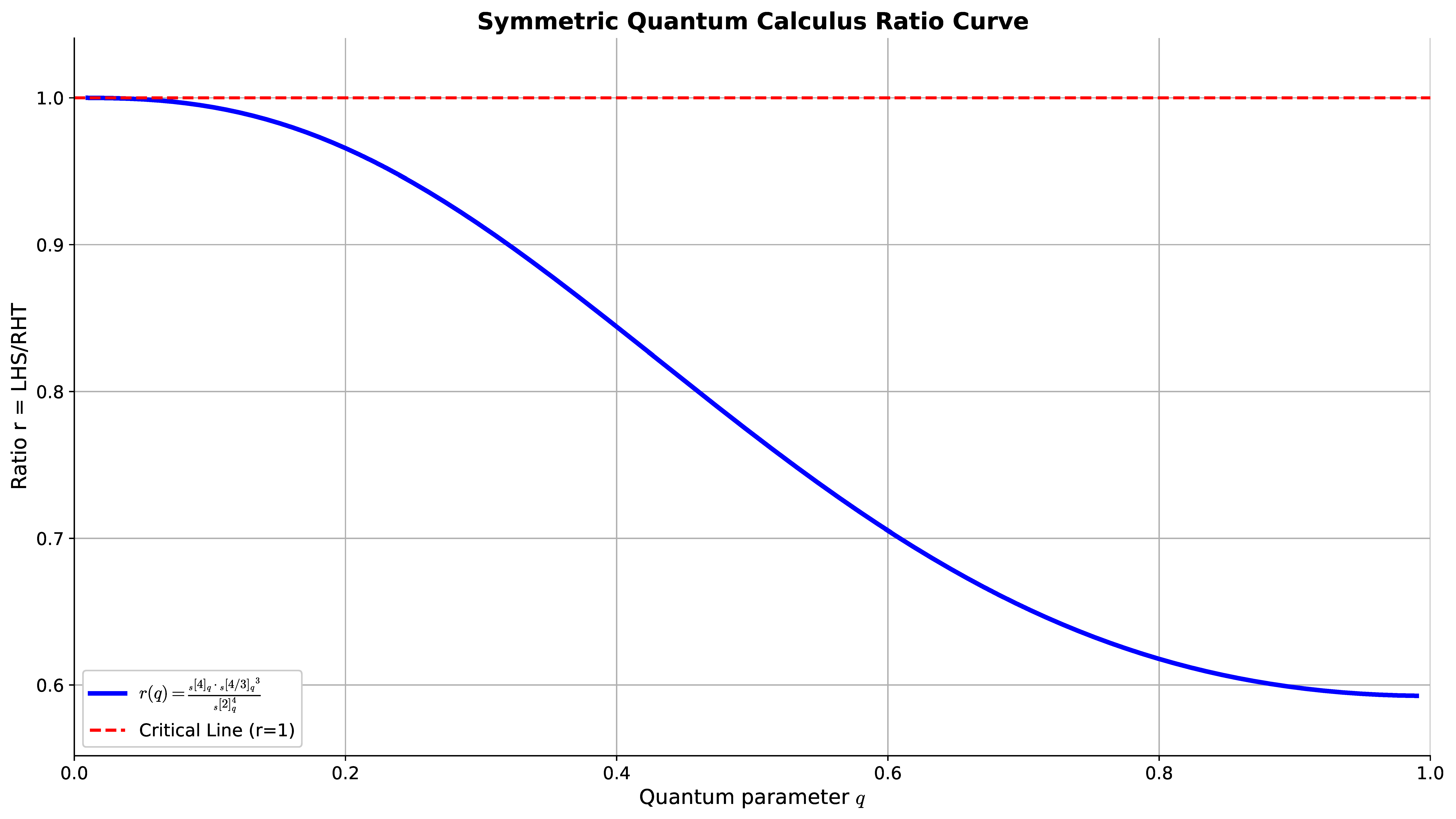
Define the ratio $r=\frac{\mathrm{LHS}}{\mathrm{RHS}}=\frac{{}_s\left[4\right]_q·{}_s[4/3]_q^3}{{}_s\left[2\right]_q^4}$. If the ratio $r\in (0,1)$, the inequality holds. We plot this ratio curve over the quantum parameter $q\in (0,1)$, as shown in Figure 1.

Figure 1 displays the ratio r as a function of q over the interval $(0,1)$. The ratio is strictly less than 1 throughout, confirming the validity of Theorem 3. Notably, for small values of q, the ratio is close to 1, implying that the upper bound is particularly tight in the strongly quantum regime. As q increases toward 1, the ratio decreases gradually but remains bounded below 1, ensuring the inequality holds for all admissible parameter values.

Now, we verify Corollary 1 using the same test function.

$$\begin{array}{cc}\hfill \mathrm{LHT}& =\frac{1}{b-a}{\int }_a^{q^{-1}b+(1-q^{-1})a}(\theta -a){}_a\mathrm{d}_q^s\theta =\frac{b-a}{q^2·{}_s\left[2\right]_q};\hfill \\ \hfill \mathrm{RHT}& =\frac{q^2·{}_s\left[2\right]_q^3}{{}_s\left[4\right]_q}{\left(\frac{1}{b-a}{\int }_a^{q^{-1}b+(1-q^{-1})a}{(\theta -a)}^{1/3}{}_a\mathrm{d}_q^s\theta \right)}^3=\frac{{}_s\left[2\right]_q^3·(b-a)}{q^2·{}_s\left[4\right]_q{·}_s{[4/3]}_q^3}.\hfill \end{array}$$

Consequently, the two inequalities in Theorem 3 and Corollary 1 share the same ratio r. We select the integration interval as $[2,5]$ and take different quantum parameters $q=0.1,0.3,0.5,0.7,0.9,0.99$. The numerical comparison for the two inequalities is presented in

Table 1. Numerical comparison of the left-hand and right-hand sides for the two symmetric quantum Favard inequalities in Example 1.

q	LHT	RHT	LHS	RHS	r
0.1	29.70297030	29.8838236	0.002970297	0.002988382	0.993948120
0.3	9.174311927	10.04873492	0.074311927	0.081394753	0.912981783
0.5	4.800000000	6.224452223	0.300000000	0.389028264	0.771152196
0.7	2.876318313	4.40339475	0.690604027	1.057255079	0.653204738
0.9	1.841620626	3.077639141	1.208287293	2.019239041	0.598387446
0.99	1.530378784	2.582282364	1.470075754	2.480530136	0.592645795

.

Table 1 provides detailed numerical values for the left and right sides of both Theorem 3 and Corollary 1, evaluated at selected discrete values of q. The results demonstrate that although the two inequalities operate over different integration intervals, their ratios r are exactly equal, which is consistent with our theoretical derivation. Furthermore, as q increases, the values on both sides increase and their differences diminish, reflecting the smooth transition to the classical integral as $q\to 1^{-}$. This numerical evidence supports the consistency and correctness of the two formulations. Here, $\mathrm{LHT}$ and $\mathrm{RHT}$ correspond to Corollary 1, while $\mathrm{LHS}$ and $\mathrm{RHS}$ correspond to Theorem 3; the last column r gives their ratio. The ratios for both forms are identical, and as $q\to 1^{-}$, the left and right sides converge.

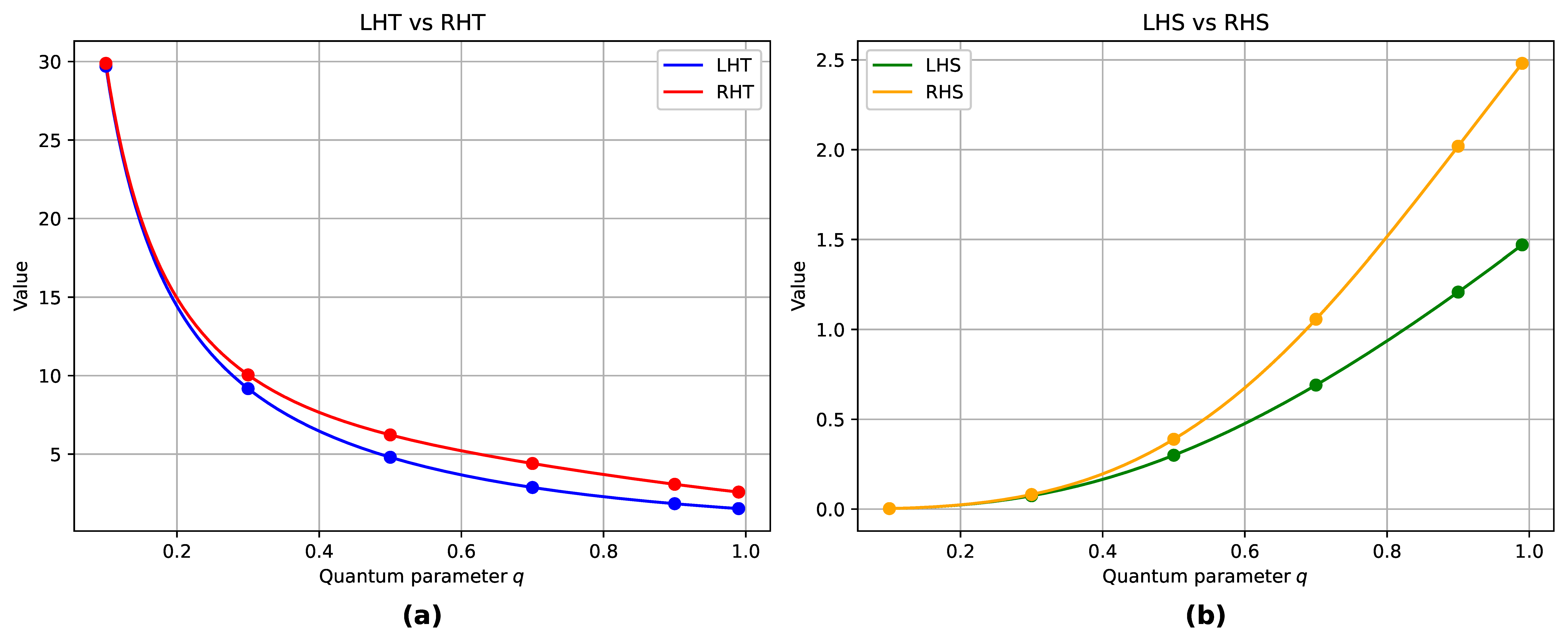
When the quantum parameter q varies continuously over the interval $(0,1)$, we obtain the curves shown in Figure 2.

Figure 2 illustrates the dependence of both sides of the symmetric quantum Favard inequality on the quantum parameter q, for the two distinct integration intervals given in Theorem 3 and Corollary 1. In each subfigure, the upper curve represents the right-hand side, which consistently dominates the lower curve representing the left-hand side. As $q\to 1^{-}$, the two curves coalesce, since the symmetric quantum integral reduces to the classical Riemann integral in the limit. Although the absolute numerical values differ between the two interval settings, their corresponding ratios remain identical, as reported in Table 1.

In [6], Yu established the q-Favard inequality (asymmetric version) in q-calculus:

$$\frac{1}{b-a}{\int }_a^b{\psi }^p\left(\theta \right){}_a\mathrm{d}_q\theta \le \frac{{\left[2\right]}_q^p}{{[p+1]}_q}{\left(\frac{1}{b-a}{\int }_a^b\psi \left(\theta \right){}_a\mathrm{d}_q\theta \right)}^p.$$

(65)

For comparison with the results of this paper, we adopt the same test function and parameters as in Example 1. Then, for the asymmetric result:

$$\begin{array}{cc}\hfill \mathrm{LHS}& =\frac{1}{b-a}{\int }_a^b{\psi }^p\left(\theta \right){}_a\mathrm{d}_q\theta =\frac{1}{b-a}{\int }_a^b(\theta -a){}_a\mathrm{d}_q\theta =\frac{b-a}{{\left[2\right]}_q};\hfill \\ \hfill \mathrm{RHS}& =\frac{{\left[2\right]}_q^p}{{[p+1]}_q}{\left(\frac{1}{b-a}{\int }_a^b\psi \left(\theta \right){}_a\mathrm{d}_q\theta \right)}^p\hfill \\ \hfill & =\frac{{\left[2\right]}_q^3}{{\left[4\right]}_q}{\left(\frac{1}{b-a}{\int }_a^b{(\theta -a)}^{\frac{1}{3}}{}_a\mathrm{d}_q\theta \right)}^3\hfill \\ \hfill & =\frac{{\left[2\right]}_q^3·(b-a)}{{\left[4\right]}_q·{[4/3]}_q^3}.\hfill \end{array}$$

Thus, the ratio for the asymmetric q-Favard inequality is:

$$r\left(q\right)=\frac{\mathrm{LHS}}{\mathrm{RHS}}=\frac{{\left[4\right]}_q·{[4/3]}_q^3}{{\left[2\right]}_q^4}.$$

(66)

For comparison, we select quantum parameter points $q=0.1,0.3,0.5,0.7,0.9,0.99$ and obtain the ratio comparison table between the symmetric and asymmetric versions, as shown in

Table 2. Numerical comparison of the ratios for the symmetric and asymmetric quantum Favard inequalities.

q	r (Symmetric Quantum)	$\mathit{r}\mathbf{\left(}\mathit{q}\mathbf{\right)}$ (Asymmetric Quantum)
0.1	0.9939481204	0.9025947625
0.2	0.9656825234	0.8093935207
0.4	0.8440658757	0.6865942807
0.6	0.7052095122	0.6252052783
0.8	0.6177911650	0.5990837399
0.9	0.5983874462	0.5940511318
0.99	0.5926457947	0.5926058939

.

For each tested value of q, the symmetric ratio is larger than the asymmetric one, confirming that the symmetric framework yields a tighter upper bound. Both ratios converge to the same value as $q\to 1^{-}$, as expected from the classical limit. Table 2 compares the ratios of the symmetric and asymmetric quantum Favard inequalities under identical test conditions. For every tested value of q, the symmetric ratio is larger than the asymmetric one, which quantitatively demonstrates that the symmetric framework provides a tighter upper bound estimate. The difference is most significant for small q (e.g., at $q=0.1$, the symmetric ratio exceeds the asymmetric one by more than $0.09$), while the two ratios converge as q approaches 1. This comparison clearly validates the advantage of the symmetric quantum calculus approach for integral upper-bound estimation.

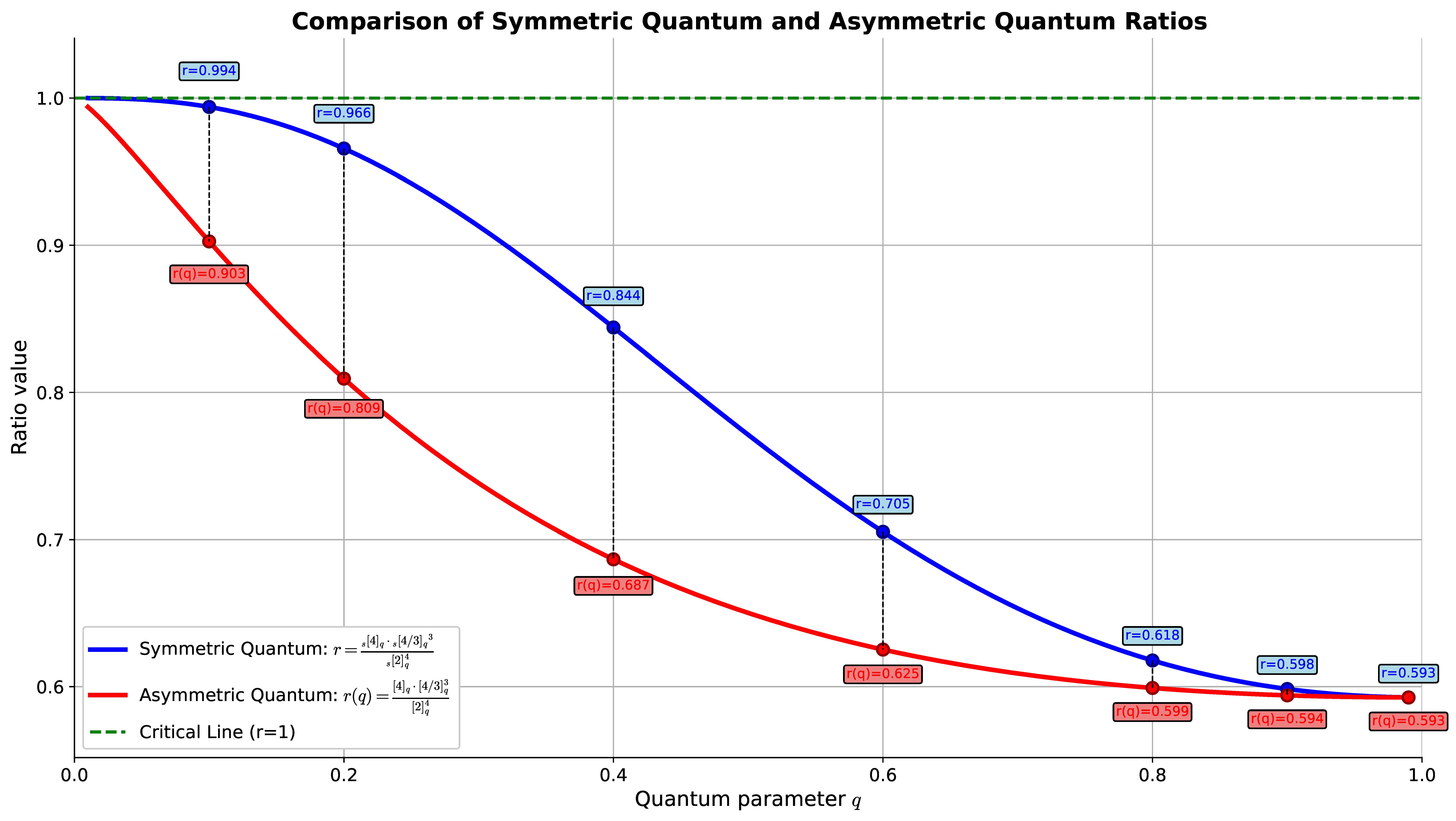
When the quantum parameter q varies continuously over the interval $(0,1)$, we obtain the ratio comparison curves shown in Figure 3.

Figure 3 presents a side-by-side comparison of the ratio r for the symmetric quantum Favard inequality (blue curve) and its asymmetric quantum counterpart (red curve). The latter is taken from the recent result of Yu [6]. Over the entire range $q\in (0,1)$, both curves lie below the horizontal line $r=1$, confirming that both inequalities are valid. More importantly, the symmetric curve is consistently higher than the asymmetric one, meaning that the symmetric inequality yields an upper bound that is closer to the true integral value. This advantage is especially pronounced for small q; for example, at $q=0.4$, the symmetric ratio is approximately $0.844$, whereas the asymmetric ratio is about $0.687$. As q approaches 1, the two curves merge, as expected from the classical limit. These observations strongly support the superiority of the symmetric quantum calculus approach.

Example 2 (Numerical verification of the symmetric quantum Berwald inequality).

Consider the function $\psi \left(\theta \right)=\sqrt[3]{\theta -a}$, which is a monotonically increasing concave function on the interval $[a,b]$. Taking $\eta =3$ and $\xi =2$, we have:

$$\begin{array}{cc}\hfill LHS& ={\left(\frac{{}_s\left[4\right]_q}{q(b-a)}{\int }_a^{qb+(1-q)a}(\theta -a){}_{a}d_q^s\theta \right)}^{\frac{1}{\eta }}={\left(\frac{{}_s\left[4\right]_q}{{}_s\left[2\right]_q}\right)}^{\frac{1}{3}}{q}^{\frac{1}{3}}{(b-a)}^{\frac{1}{3}};\hfill \\ \hfill RHS& ={\left(\frac{{}_s\left[3\right]_q}{q(b-a)}{\int }_a^{qb+(1-q)a}{(\theta -a)}^{\frac{2}{3}}{}_{a}d_q^s\theta \right)}^{\frac{1}{2}}={\left(\frac{{}_s\left[3\right]_q}{{}_s[5/3]_q}\right)}^{\frac{1}{2}}{q}^{\frac{1}{3}}{(b-a)}^{\frac{1}{3}}.\hfill \end{array}$$

Thus, the ratio is:

$$r=\frac{\mathrm{LHS}}{\mathrm{RHS}}={\left(\frac{{}_s\left[4\right]_q}{{}_s\left[2\right]_q}\right)}^{\frac{1}{3}}·{\left(\frac{{}_s[5/3]_q}{{}_s\left[3\right]_q}\right)}^{\frac{1}{2}}.$$

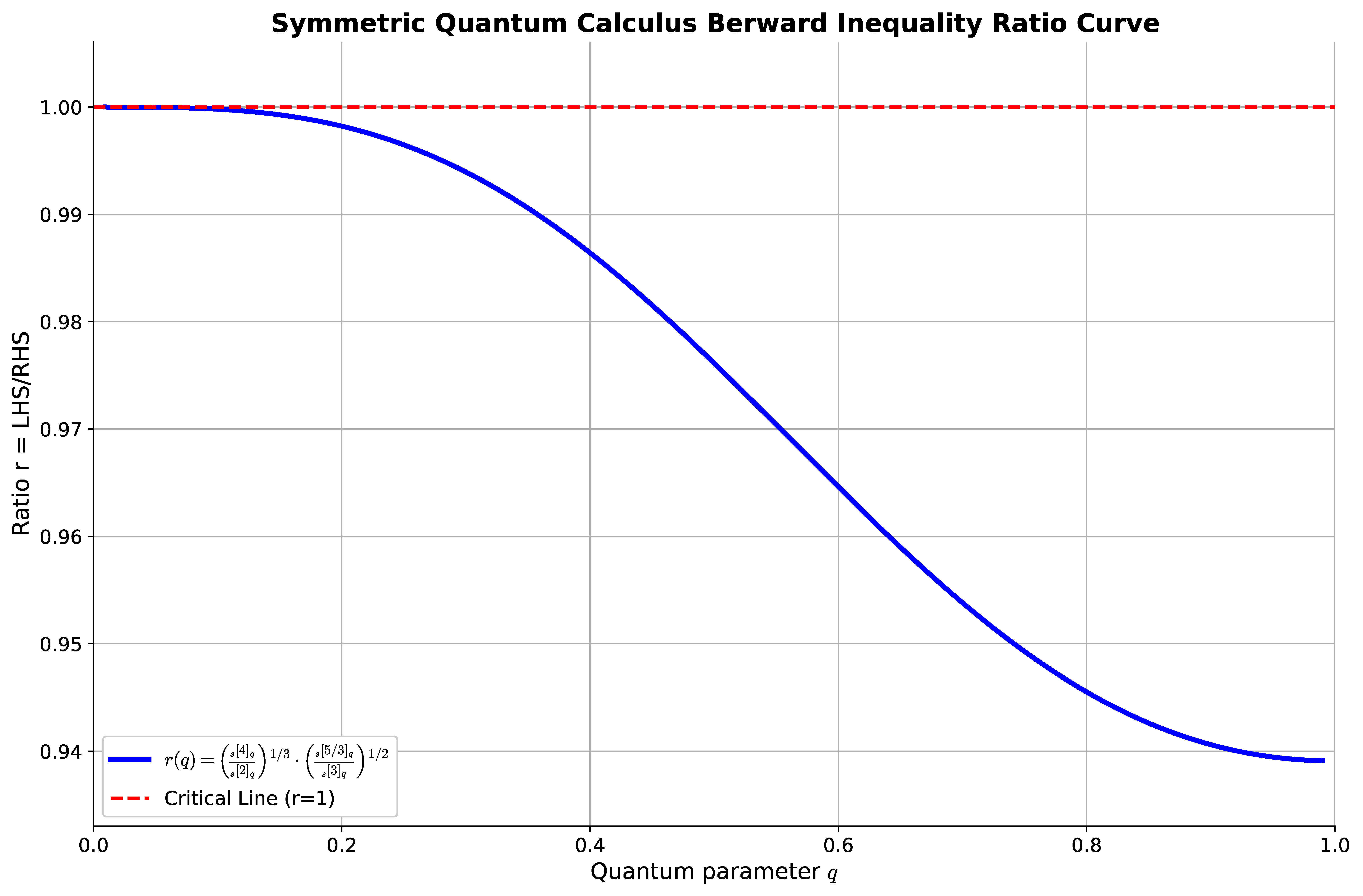
Similarly, we visualize this ratio curve over $q\in (0,1)$, as shown in Figure 4.

Figure 4 shows the ratio r for the symmetric quantum Berwald inequality established in Theorem 7, plotted against the quantum parameter q. The curve lies strictly below 1 for all $q\in (0,1)$, verifying the validity of the Berwald-type inequality in the symmetric quantum setting. The ratio decreases monotonically with q, indicating that the gap between the two sides expands as q increases. In the limit $q\to 0^{+}$, the ratio approaches 1, suggesting that the estimate is extremely sharp in the strongly quantum regime. This behavior is consistent with the theoretical predictions and further demonstrates the utility of the symmetric quantum framework.

The symmetric quantum Favard inequality established in this paper can be potentially applied to energy estimation problems in sensor networks. Consider a linear array of wireless sensor nodes deployed along a one dimensional interval $[a,b]$. Due to hardware constraints or intentional non-uniform clustering, the node positions follow the symmetric quantum lattice

$${\theta }_n=q^{2n+1}b+(1-q^{2n+1})a,n=0,1,2,\cdots ,$$

which is precisely the evaluation node set of the symmetric quantum integral (2.5). The quantum parameter $q\in (0,1)$ controls the concentration of nodes near the endpoint a: as $q\to 0$ the nodes accumulate near a, while as $q\to 1$ they tend to be uniformly distributed. The symmetry of this distribution, reflected by the duality $q\leftrightarrow q^{-1}$, guarantees balanced coverage when the network operates simultaneously in forward and backward directions.

Suppose the energy consumed by a node located at $\theta$ is given by a non-negative, concave and increasing function $\psi \left(\theta \right)$, which often originates from signal attenuation laws or data fusion costs. A typical example is $\psi \left(\theta \right)=\sqrt[3]{\theta -a}$, capturing the cube-root characteristic of distance-dependent path loss. The network operator is interested in the p-th moment of energy consumption, which can be expressed via the symmetric quantum integral as

$$E_p^{\left(s\right)}[a,qb+(1-q)a]=\frac{1}{q(b-a)}{\int }_a^{qb+(1-q)a}{\psi }^p\left(\theta \right){}_a\mathrm{d}_q^s\theta .$$

For large-scale deployments, computing this moment exactly may be costly; hence a tight upper bound is highly valuable for capacity planning and worst-case analysis.

By Theorem 3, since $\psi \left(\theta \right)$ satisfies all the required conditions, we immediately obtain the analytic upper bound

$$E_p^{\left(s\right)}\le B_p^{\left(s\right)}:=\frac{{}_s\left[2\right]_q^p}{{}_s[p+1]_q}{\left(\frac{1}{q(b-a)}{\int }_a^{qb+(1-q)a}\psi \left(\theta \right){}_a\mathrm{d}_q^s\theta \right)}^p.$$

This bound depends only on the average energy consumption $E^{\left(s\right)}$ and the symmetric quantum integers ${}_s[·]_q^p$, and can be computed directly from the node positions without explicitly summing over all sensors.

Compared with the asymmetric counterpart, Table 2 lists the ratios for various values of q. The symmetric quantum inequality consistently gives ratios closer to 1, implying a tighter upper bound and therefore greater practical value for resource provisioning. For instance, at $q=0.4$ the symmetric bound exceeds the true value by only about $15.6\%$ (i.e., $1-r\approx 0.156$), whereas the asymmetric bound exceeds it by about $31.4\%$. Such a difference can translate into substantial energy savings in network design.

When it is necessary to compare energy consumption at two different orders $\eta >\xi >0$ (e.g., peak power versus average power), the symmetric quantum Berwald inequality (Theorem 7) provides the relation:

$${\left({}_s[\eta +1]_q{E}_{\eta }^{\left(s\right)}\right)}^{1/\eta }\le {\left({}_s[\xi +1]_q{E}_{\xi }^{\left(s\right)}\right)}^{1/\xi }$$

in which only measurable average quantities are required. Using this relation, the operator can infer the worst-case peak energy from the average consumption without detailed node-level monitoring.

Symmetric quantum lattices arise naturally in systems that are invariant under the exchange $q\leftrightarrow q^{-1}$, such as certain topological insulator edge states or discretised models with built-in particle-hole symmetry. The Favard-type inequalities established in this work provide a rigorous mathematical tool for energy estimation in such platforms, and as demonstrated above, the symmetric formulation consistently yields tighter upper bounds than its asymmetric counterpart, offering a notable advantage.

5. Conclusions

In this paper, we have systematically established, for the first time, the theory of Favard-type and Berwald-type inequalities within the framework of symmetric quantum calculus. This work fills a notable gap in the literature, as previous studies on quantum integral inequalities were predominantly confined to the asymmetric quantum setting, while the symmetric counterpart, which naturally preserves the duality $q\leftrightarrow q^{-1}$, remained largely unexplored in the context of Favard-type estimates. The results obtained herein not only enrich the theoretical landscape of symmetric quantum calculus but also provide practical tools for obtaining sharper upper bounds in discrete integral estimation problems.

The main theoretical contributions of this paper are threefold. First, we established a fundamental comparison lemma (Lemma 3) based on symmetric quantum monotonicity, which serves as a cornerstone for deriving subsequent inequalities. Second, building upon this lemma, we derived the symmetric quantum Favard inequality (Theorem 3) and its extended version for functions for which ${\psi }^{1/\delta }$ is concave (Theorem 4), thereby substantially broadening the class of admissible functions beyond the classical concave setting. Third, we obtained generalized inequalities for products of multiple functions (Theorems 5 and 6) and established the symmetric quantum Berwald inequality (Theorems 7 and 8), providing a complete framework for comparing integral means of different orders. These results collectively form a coherent theory of Favard–Berwald-type inequalities in symmetric quantum calculus.

Numerical examples and comparative analyses further substantiate the theoretical findings. For the test function $\psi \left(\theta \right)=\sqrt[3]{\theta -a}$, our results demonstrate that the symmetric quantum framework consistently yields upper bound estimates that are closer to the true integral values than those obtained from the asymmetric quantum setting, particularly for small values of the quantum parameter q. This advantage is quantitatively reflected in the ratios presented in Table 2, where the symmetric ratios are uniformly larger than their asymmetric counterparts across the entire range $q\in (0,1)$. These observations not only verify the correctness of the established inequalities but also highlight the practical superiority of the symmetric approach.

Several promising directions warrant further investigation. First, the establishment of weighted symmetric quantum Favard and Berwald inequalities would extend the applicability of the present results to a broader class of problems involving non-uniform measures. Second, exploring reverse inequalities, i.e., lower bound estimates, within the symmetric quantum framework remains an open problem of both theoretical and practical interest. Third, constructing novel symmetric quantum integral-type operators and analyzing their approximation–theoretic properties could bridge the gap between the present theory and applications in numerical analysis and signal processing. Fourth, the extension of the current results to $(p,q)$-symmetric quantum calculus or to higher-dimensional settings may yield new insights. We believe that further exploration along these directions will significantly advance the development of symmetric quantum calculus and foster its integration with related fields such as computational mathematics, convex analysis, and mathematical physics.

References

1. Favard, J. Sur les valeures moyennes. Bull. Sci. Math. 1933, 57, 54–64. [Google Scholar]
2. Maligranda, L.; Pečarić, J.E.; Persson, L.E. Weighted Favard and Berwald inequalities. J. Math. Anal. Appl. 1995, 190, 248–262. [Google Scholar] [CrossRef] [Scilit]
3. Kac, V.; Cheung, P. Quantum Calculus; Springer: New York, NY, USA, 2001. [Google Scholar]
4. Mishra, O.; Porwal, S. Quantum approach on linear combination of harmonic univalent mappings. arXiv 2021, arXiv:2108.04714. [Google Scholar] [CrossRef] [Scilit]
5. Mursaleen, M.A.; Kilicman, A.; Nasiruzzaman, M. Approximation by q-Bernstein-Kantorovich operators with shiftedknots of real parameters. Filomat 2022, 36, 1179–1194. [Google Scholar] [CrossRef] [Scilit]
6. Yu, J. Quantum integral Favard-type inequality. Appl. Math. Comput. 2025, 500, 129452. [Google Scholar] [CrossRef] [Scilit]
7. Yunus, A.O.; Olanrewaju, O.A. Fractional-order modeling and optimal control of lassa fever with non-pharmaceutical interventions. MethodsX 2026, 16, 103932. [Google Scholar] [CrossRef] [Scilit] [PubMed]
8. Yunus, A.O.; Olanrewaju, O.A. Fractional-order modeling of vaccination strategies for measles transmission incorporating immune memory. Virus Res. 2026, 367, 199718. [Google Scholar] [CrossRef] [Scilit] [PubMed]
9. Yunus, A.O.; Olayiwola, M.O. A mathematical model for assessing vaccination’s efficacy as a preventative strategy against newly emerging COVID-19 variants. Vacunas 2025, 26, 500392. [Google Scholar] [CrossRef] [Scilit]
10. Yunus, A.O. Modeling and analysis of microbial dynamics in malaria and measles co-infections with public awareness interventions via numerical simulation. Microbe 2025, 9, 100613. [Google Scholar] [CrossRef] [Scilit]
11. Yunus, A.O.; Olayiwola, M.O. Mathematical modeling of malaria epidemic dynamics with enlightenment and therapy intervention using the Laplace-Adomian decomposition method and Caputo fractional order. Frankl. Open 2024, 8, 100147. [Google Scholar] [CrossRef] [Scilit]
12. Yunus, A.O.; Olayiwola, M.O.; Abanikanda, M.O. Modeling a fractional-order chlamydia dynamic with protected intimacy as a strategic control intervention. Discov. Public Health 2025, 22, 491. [Google Scholar] [CrossRef] [Scilit]
13. Bilal, M.; Iqbal, A.; Rastogi, S. Quantum symmetric analogues of various integral inequalities over finite intervals. J. Math. Inequal. 2023, 17, 615–627. [Google Scholar] [CrossRef] [Scilit]
14. Vivas-Cortez, M.; Javed, M.Z.; Awan, M.U.; Dragomir, S.S.; Zidan, A.M. Properties and Applications of Symmetric Quantum Calculus. Fractal Fract. 2024, 8, 107. [Google Scholar] [CrossRef] [Scilit]
15. Nosheen, A.; Ijaz, S.; Khan, K.A.; Awan, K.M.; Albahar, M.A.; Thanoon, M. Some q-symmetric integral inequalities involving s-convex functions. Symmetry 2023, 15, 1169. [Google Scholar] [CrossRef] [Scilit]
16. Liu, Q.; Javed, M.Z.; Awan, M.U.; Ciurdariu, L.; Alkahtani, B.S. Hermite-Hadamard’s like inequalities via symmetric quantum calculus. Ain Shams Eng. J. 2025, 16, 103372. [Google Scholar] [CrossRef] [Scilit]
Figure 1. Ratio curve r = LHS / RHS of the symmetric quantum Favard inequality in Example 1 as a function of the quantum parameter q ( 0 , 1 ) . The ratio remains below 1 for all q, verifying the validity of Theorem 3; the closer r is to 1, the tighter the upper bound estimate. For small q, the ratio approaches 1, indicating sharper estimates in the strongly quantum regime.
Symmetry 18 01156 g001
Figure 2. Comparison of the left-hand side (LHS) and right-hand side (RHS) of the symmetric quantum Favard inequality as functions of q. Subfigure (a) corresponds to the interval [ a , q b + ( 1 q ) a ] (Theorem 3), and subfigure (b) corresponds to [ a , q 1 b + ( 1 q 1 ) a ] (Corollary 1). In both panels, the solid curves represent the LHS and the dashed curves represent the RHS. The RHS always lies above the LHS, and both sides converge as q 1 , consistent with the classical limit.
Symmetry 18 01156 g002
Figure 3. Comparison of the ratio r for the symmetric quantum Favard inequality (upper blue curve) and the asymmetric quantum Favard inequality (lower red curve). Both curves remain below 1, confirming the validity of both inequalities. However, the symmetric curve consistently lies above the asymmetric one over the entire range q ( 0 , 1 ) , demonstrating that the symmetric quantum framework provides tighter upper bounds than its asymmetric counterpart.
Symmetry 18 01156 g003
Figure 4. Ratio curve r = LHS / RHS of the symmetric quantum Berwald inequality in Example 2 as a function of q ( 0 , 1 ) . The ratio remains below 1 for all q, verifying Theorem 7. As q increases, the ratio decreases monotonically, indicating that the gap between the two sides widens as the quantum parameter approaches 1.
Symmetry 18 01156 g004