Hierarchical TSK Fuzzy Classification Through Positive Intervention for Teaching Evaluation

Abstract

Currently, most existing traditional teaching evaluation models are difficult to truly reflect the contribution and guiding role of administrative policies in teaching decision-making, and lack the interpretability of teaching semantics in assessing actual teaching methods and effectiveness. In addition, the substantive strategies of intervention are also difficult to quantify and evaluate. This study proposes a hierarchical Takagi–Sugeno–Kang (TSK) fuzzy classification model (Pgt-TC) with positive intervention guidance ability. The study stacks several interpretable zero-order TSK fuzzy classifiers as the basic training units (BTUs), ensuring that the final model has high interpretability of teaching semantics. Firstly, the fuzzy rule base corresponding to BTUs is determined according to the contribution level of each rule, and residual is used to reduce the error interference between adjacent BTUs, achieving the goal of improving the generalization ability of the training model. In addition, this study designed a strategy to generate posterior parameters by solving the approximation error of adjacent BTUs, which improved the classification and generalization performance of the fuzzy system. The proposed model is evaluated on five datasets, including one core educational research dataset (177 samples, 19 features) and four UCI benchmark datasets (163–5000 samples, 4–27 features). Results are reported using 5-fold cross-validation with mean values. Experimental results show that Pgt-TC achieves competitive classification performance across all datasets. On the educational dataset, it attains an average test accuracy of 93.47 and an average test SE value of 98.60, while also offering interpretability to explain educational intervention decisions.

1. Introduction

The digitalization of educational resources is profoundly reshaping the global education ecosystem and has become a core driving force in promoting teaching reform. Digital technologies provide systematic solutions for the transformation of educational modernization by expanding the supply of high-quality resources, innovating teaching models, and enhancing educational quality. UNESCO notes in the 2024 Global Education Monitoring Report (GEMR) that digital technologies are redefining the control and quality of education, offering technical support to bridge educational gaps by expanding resource coverage and facilitating personalized learning [1]. The OECD’s policy survey on the digital transformation of schooling indicates that over 60% of countries have developed dedicated strategies for educational digitalization, driving holistic changes in education systems [2]. According to the China smart education development report (2024–2025), the national smart education platform has surpassed 164 million registered users. By adopting an integrated, intelligent, and international (i.e., III) approach, digital technologies have been deeply integrated into the entire teaching process, effectively addressing issues such as uneven resource distribution and shortages of high-quality teachers [3]. Educational digitalization is transitioning from instrumental application to systemic transformation. Its core value lies in expanding educational opportunities and optimizing resource allocation through technological means, ultimately realizing the vision of lifelong learning where “everyone can learn, everywhere can be a place of learning, and learning can happen at any time.” This transformation is not merely an emergency response to current challenges, but a strategic choice for the future of education.

Under the traditional digital educational resource application model, related research primarily revolves around three core directions. In the research on teaching evaluation indicator systems, scholars attempt to quantify teaching effectiveness and provide basis for resource optimization by establishing multi-dimensional, multi-level evaluation frameworks. Chen L. et al. proposed a “four-dimensional evaluation model for digital teaching resources” [4], constructing a systematic evaluation system from technical, pedagogical, usability, and sustainability dimensions. Yin H. et al. constructed a smart classroom evaluation indicator system [5], establishing operable evaluation criteria covering seven first-level dimensions such as smart environment, smart resources, and smart teaching activities. Of course, most of these methods lack the ability to capture teaching policies during the teaching process, and are also difficult to truly reflect real-time interactions and dynamic changes in the teaching process.

In teaching process intervention research, scholars primarily employ digital means to intervene in and optimize teaching implementation processes. Baker et al. proposed a “learning analytics-based teaching intervention model” [6], achieving dynamic intervention decisions through real-time monitoring of learning behavior data. Chen Li et al. developed a “smart teaching intervention mechanism” [7], constructing a teaching intervention framework based on multi-source data fusion. However, intervention strategies suffer from a “black box” problem, with most intervention models lacking interpretability.

In teaching intervention effectiveness research, the focus is on validating the actual effects of digital teaching interventions. Hattie verified the effectiveness of various teaching intervention strategies through meta-analysis [8], while Zhang Yi et al. conducted empirical research on intelligent teaching intervention effects, validating the differences in effectiveness among different intervention models through comparative experiments [9]. However, the evaluation dimensions are overly simplified, lacking long-term tracking and sustainability verification of intervention effects.

Previous applications of fuzzy theory in teaching [10,11,12] have been limited, the direct integration of fuzzy methods into teaching interventions remains even scarcer [13]. Meanwhile, although TSK (Takagi–Sugeno–Kang) fuzzy classifiers have been applied to student performance prediction and dropout early warning due to their superior nonlinear mapping capabilities and rule interpretability [14,15], they have not yet been sufficiently extended to the hierarchical modeling of teaching behavior intervention indicators or to reflective evaluation feedback grounded in the OBE (Outcome-Based Education) philosophy.

Guided by the OBE philosophy, this study addresses the incompleteness of behavioral objectives, the untimely feedback in evaluation, and the shortcomings in data analysis within the teaching assessment process.

By expanding behavioral intervention indicators and providing reflective evaluation, a hierarchical TSK fuzzy classifier is designed to leverage its high performance and strong interpretability in resolving these issues. Based on the above considerations, this study proposes a novel hierarchical fuzzy classifier.

This study proposes a new rule generation algorithm that fully explores and screens important rules in the current training unit, and transfers the key information characterized by these rules to the next training unit, effectively improving the model’s generalization ability.

The original input space of the model proposed in this study differs from that of other models. The input space consists of two subspaces: the first subspace serves as the fundamental input space and simultaneously constitutes the output space of the initial basic building unit. The second subspace is formed by augmenting the first subspace with four additional features, and it functions as the original input space for the second basic building unit, as well as all subsequent basic building units. The true labels for the overall input space are manually assigned based on the characteristics of the first subspace (i.e., the input subspace before feature augmentation). The construction of the second subspace (the input subspace after feature augmentation) aims to enhance the descriptive capacity of the input space for each sample. The decision not to directly employ the second subspace as the entire model’s input space is intended to verify whether these newly added features can effectively assist schools in identifying students who require teaching process interventions.

To ensure that the input space of each basic building unit shares the same physical interpretation, thereby enhancing the overall interpretability of the model, this study proposes a novel method for constructing the input space. This method projects the residual between the output of the current basic building unit and the output of the first basic building unit onto the original input space (where the original input space refers to the second input subspace mentioned above).

In order to ensure consistency in approximation ability between different training units, this study proposes an optimization method for solving model output weights by reducing error accumulation.

This study will begin by systematically reviewing existing research achievements and theoretical foundations. Based on this groundwork, a research model will be constructed, and the validity of the model will be verified and analyzed through multi-dimensional experimental data. Ultimately, conclusions with both theoretical support and practical value will be drawn.

The rest of this study is structured as follows. Section 2 covers materials and methods, including the baseline TSK classifier, the proposed Pgt-TC model, its training algorithm, complexity, and comparisons. Section 3 presents experiments, results, and analyses. Section 4 is the conclusion, including a summary of this study and future outlook.

2. Materials and Methods

Generally, fuzzy neural networks possess stronger interpretability and generalization performance compared to traditional neural networks. Therefore, most researchers typically aim to further improve fuzzy neural networks in terms of both generalization performance and interpretability. In our previous work, we developed an interpretable multi-level stacked-structure TSK fuzzy classifier, D-TSK-FC [16], which is constructed by stacking zero-order TSK fuzzy classifiers layer by layer. This model uses the random offset of the predicted output from the current layer combined with the original data space to form the input for the next layer. This approach not only ensures that the input at each layer maintains the same physical interpretation as the original data space but also enhances the model’s generalization performance. Other researchers have also approached the improvement of interpretability and generalization performance from different perspectives, such as Xie [17], who proposed a TSK fuzzy classifier that does not require any clustering strategy. Since no clustering strategy is employed, each sub-classifier is trained in parallel, and the researchers developed a corresponding incremental learning algorithm to dynamically update the model structure. Compared to certain traditional models that rely on aggregation methods such as weighting or averaging, this structure offers higher interpretability and generalization performance. The model proposed in this study is a multi-level TSK fuzzy neural network based on zero-order TSK fuzzy classifiers. Therefore, before introducing the proposed model in detail, we first review the zero-order TSK fuzzy classifier.

2.1. Classical Zero-Order TSK Fuzzy Classifier

Typically, TSK fuzzy classifiers are categorized into first-order and zero-order types. Although the zero-order TSK fuzzy classifier may sacrifice some performance compared to its first-order counterpart, it offers more concise interpretability. This aspect is of significant practical importance for this study, particularly when analyzing scenarios before and after feature augmentation. Furthermore, the model proposed in this research can substantially compensate for the performance loss inherent in the zero-order TSK fuzzy classifier. Therefore, this study adopts the zero-order TSK fuzzy classifier as the fundamental building unit of the model.

The expression for the k-th fuzzy rule is given as follows [18]:

$$\begin{array}{l}{R}_k:\mathrm{IF} {\mathit{x}}_1 is A_1^k and{ \mathit{x}}_2 is A_2^k and \dots and{ \mathit{x}}_j is A_j^k and\dots and x_d is A_d^k,\\ \mathrm{THEN} {\mathrm{y}}_k=p_0^k,k=1,2,\dots \dots K,\end{array}$$

where $x_j$ represents the j-th feature, $R_k$ denotes the k-th rule, $A_j^k$ is the fuzzy set corresponding to the input vector $\mathbf{x}$ in the k-th rule, and $p_0^k$ indicates the output corresponding to the k-th fuzzy rule.

The final output is then obtained through a series of operations and defuzzification [19].

$$y_0={\displaystyle \frac{{\displaystyle \sum _{k=1}^K{\mu }^k(x)p_0^k}}{{\displaystyle \sum _{k=1}^K{\mu }^{k^{\prime }}(x)}}}={\displaystyle {\displaystyle \sum _{k=1}^K}{\tilde{\mu }}^k(x)p_0^k=}{\displaystyle {\displaystyle \sum _{k=1}^K}{\mu }^k(x)p_0^k}$$

(1)

Here, ${\mu }^k(x)$ can be expressed as Equation (2):

$${\mu }^k(x)={\displaystyle \prod _{i=1}^d{\mu }_{A_i}^k(x_i)}$$

(2)

and ${\tilde{\mu }}^k(x)$ can be represented as Equation (3):

$${\tilde{\mu }}^k(x)={\displaystyle \frac{{\mu }^k(x)}{{\displaystyle \sum _{k^{\prime }=1}^K{\mu }^{k^{\prime }}(x)}}}$$

(3)

Membership functions typically come in various shapes, such as triangular membership functions [20], trapezoidal membership functions [21], Gaussian membership functions [22], and so on. Since Gaussian membership functions are differentiable everywhere, this study adopts the most commonly used Gaussian membership function as the membership function for fuzzy rules [16,17]. Its expression is given by Equation (4):

$${\mu }_{A_i}^k(x_i)=\exp ({\displaystyle \frac{-{(x_i-c_i^k)}^2}{2{\delta }_i^k}})$$

(4)

Here, ${\mu }_{A_i}^k(x_i)$ represents the membership degree of the j-th feature in the k-th fuzzy rule. The parameters $c_i^k$ and ${\delta }_i^k$ are obtained through FCM [23] or other clustering algorithms.

2.2. Training Model Construction

In this section, we will elaborate on the specific structure of the model and the optimization approach for the basic building units. The optimization problem for the basic building units typically aims to minimize the error between the predicted output and the actual labels. In order to ensure consistency in approximation ability between different basic building units, this study proposes an optimization method for solving model output weights by reducing error accumulation.

2.2.1. Optimization of Antecedent Parameters in the Basic Building Units

The basic building unit of the model proposed in this study is a zero-order TSK fuzzy classifier. To better adapt it to the specific problem addressed in this research, the improvement and optimization of its antecedent parameters are considered as follows:

In previous studies, researchers commonly employed Gaussian functions as membership functions and predefined the number of fuzzy partitions. For example, Zhou et al. [16] divided the fuzzy interval into five equally spaced fuzzy partitions, with the centers of membership fixed at [0, 0.25, 0.5, 0.75, 1], and assigned physical meanings to each partition. Additionally, in some studies, researchers used clustering algorithms such as FCM to generate the centers and variances of the fuzzy partitions. While these methods ensure concise interpretability for each fuzzy partition, this study specifically focuses on the problem of teaching process intervention. If the antecedent parameters are set manually or arbitrarily, it remains uncertain whether such parameters can achieve optimal model performance for teaching process intervention. Therefore, building upon previous methods, this study proposes a novel approach for generating antecedent parameters.

Considering that an excessive number of fuzzy partitions may increase the computational cost of the model and complicate the fuzzy rules, thereby reducing interpretability, this study sets the number of fuzzy partitions to five. Gaussian membership functions are adopted for these partitions. The cluster centers for each fuzzy partition are determined using the FCM algorithm, and the physical meanings of these cluster centers are defined as “very low,” “low,” “medium,” “high,” and “very high,” respectively. This approach ensures the interpretability of the zero-order TSK fuzzy classifier.

The Gaussian membership function value for the j-th feature of the i-th sample is calculated by the expression:

$${\mu }_j^i(x_{ij},c)=\exp (-{(x_{ij}-a_c)}^2/2{\sigma }_c^2),$$

where $a_c$ denotes the k-th fuzzy cluster center, ${\sigma }_c^2$ is the variance, and both $a_c$ and ${\sigma }_c^2$ are generated by the FCM algorithm.

Additionally, this study employs a weighted average of the C Gaussian membership function values for each feature $x_{ij}$, expressed as Equation (5):

$${\mu }_{\mathit{ij}}={\displaystyle \frac{{\displaystyle \sum _{r=1}^C{\mu }_j^i(x_{ij},c)D_{\mu }\left({\mu }_j^i(x_{ij},c)\right)}}{{\displaystyle \sum _{r=1}^C{D}_{\mu }\left({\mu }_j^i(x_{ij},c)\right)}}}$$

(5)

which is then used to construct a feature membership matrix ${\mathsf{\mu }}_{N\times \mathit{d}}$, where N denotes the number of samples and d represents the number of features.

Subsequently, based on the obtained feature membership matrix ${\mathsf{\mu }}_{N\times \mathit{d}}$, the output weight of each rule for every sample is calculated and expressed as Equation (6):

$$W_i^l={\displaystyle {\displaystyle \prod _{j=1}^d}\mathit{\mu }(\mathit{i},\mathit{j})}\times \mathit{\psi }(\mathit{j},\mathit{l})$$

(6)

where $\mathit{\psi }(\mathit{j},\mathit{l})$ is an information certainty matrix, $l$ denotes the number of rules, and each element of this matrix is a random number within the interval [0, 1].

Finally, based on the rule output weights, a rule output matrix can be expressed as:

$$\mathbf{H}={\left(\begin{array}{ccc}{\omega }_{11}& \dots & {\omega }_{1l}\\ ⋮& \ddots & ⋮\\ {\omega }_{N1}& \dots & {\omega }_{Nl}\end{array}\right)}_{N\times l}$$

(7)

2.2.2. Optimization of Consequent Parameters

Given two datasets $D_1\{{\mathit{x}}_i,y_i\}$ and $D_2\{{\mathit{x}}_j,y_j\}$, where $i=1,2,\cdots ,N_1$, $j=1,2,\cdots ,N_2$ and $N_1<N_2$. Here, ${\mathit{x}}_i$ and ${\mathit{x}}_j$ represent the input samples of the two datasets, while $y_i$ and $y_j$ denote the corresponding labels of the input samples. Since the main objective of this study is to distinguish between students who require academic intervention and those who do not by analyzing their academic performance, the labels are binary, represented as $y_i\in \{+1,-1\}$, $y_j\in \{+1,-1\}$. Let ${\mathbf{X}}_1=[x_1,x_2,\cdots ,x_{N_1}]$, ${\mathbf{T}}_1=[y_1,y_2,\cdots ,y_{N_1}]$; ${\mathbf{X}}_2=[x_1,x_2,\cdots ,x_{N_2}]$, ${\mathbf{T}}_2=[y_1,y_2,\cdots ,y_{N_2}]$, given that both datasets describe the academic performance of the same group of students, the labels for the two datasets are identical and are uniformly denoted here as $\mathbf{T}$.

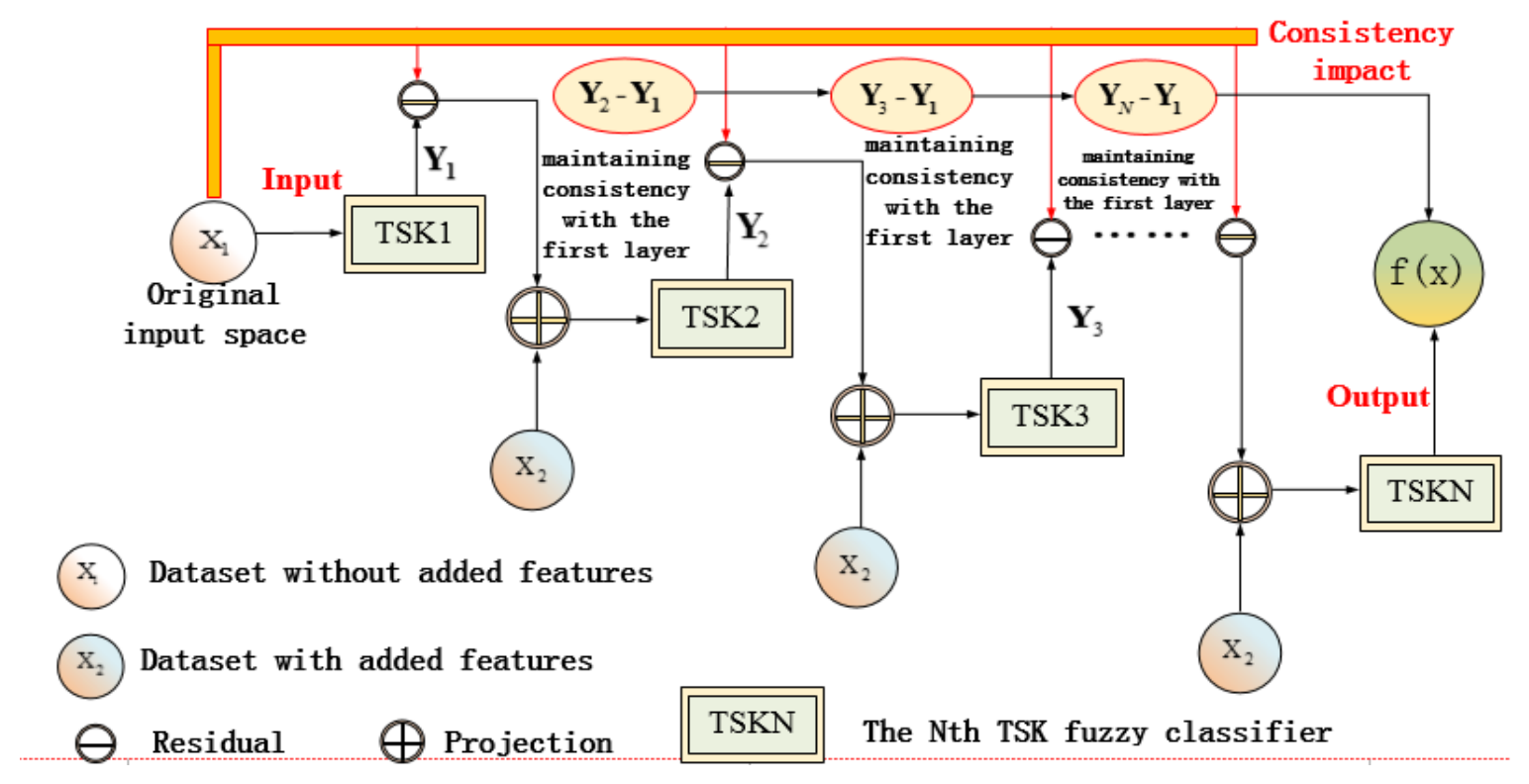
This study aims to analyze whether newly added features can enhance the description of original samples through a fuzzy classifier. Therefore, it is necessary to compare the classification performance before and after the addition of features. Accordingly, the input to the first-layer basic building unit of the proposed multi-level fuzzy classifier consists of the original samples, while the inputs to subsequent basic building units are the sample spaces after the addition of features. By comparing the performance of the classifier before and after feature augmentation, we ultimately determine whether the added features in the dataset can better describe students’ academic performance as a whole. On this basis, this study attempts to improve the overall generalization ability of the model through a stacked structure. The model’s structure can be referred to in Figure 1.

Figure 1 shows the Pgt-TC architecture. The data flow is as follows: (1) Subspace 1 samples enter BTU₁, producing initial predictions via FCM-based TSK rules. (2) Subspace 2 samples (four extra features) feed BTU₂ and later BTUs. (3) For each BTU (td ≥ 2), the input is the residual between its output and BTU₁’s output, projected onto Subspace 2 with a random offset. (4) Each BTU’s output weights are optimized to minimize both local error and discrepancy with adjacent BTUs. (5) Final classification aggregates all BTU outputs.

Ridge regression [24,25] is an improved linear regression algorithm used to compute the consequent parameter weights. In the first and second basic building units of this study, we directly employ ridge regression to calculate the output weight parameters. Next, we will focus on introducing the computation process of consequent parameters for other basic building units.

If each subsequent basic building unit uses ridge regression to compute the consequent parameters, then, while these subsequent units can reflect the relationship before and after feature augmentation to some extent based on the stacked structure, this relationship is confined to the input space. Therefore, the proposed new method for computing consequent parameters in the basic building units needs to ensure consistency with the first and second basic building units. We aim to enhance the classification performance of the model by strengthening consistency among the units.

First, the objective function is defined, which is similar to that in [26]. In order to enhance the generalization ability of the model, this study considers both the consistency between different basic building units and the approximation ability and differences between different basic building units when setting the objective function. Based on the above analysis, we provide the following definition.

Definition 1.

$$F_{\mathit{td}}=({\mathbf{H}}_{\mathit{td}}{\mathbf{\beta }}_{\mathit{td}}-\mathbf{T}{)}^2+{\lambda }_1({\mathbf{H}}_{\mathit{td}}{\mathbf{\beta }}_{\mathit{td}}-{\mathbf{Y}}_1{)}^2+{\lambda }_2({\mathbf{H}}_{\mathit{td}}{\mathbf{\beta }}_{\mathit{td}}-{\mathbf{Y}}_{\mathit{td}-\mathbf{1}}{)}^2$$

(8)

Solution Steps for Equation (1) are provided in the proof below.

Proof. 

In order to achieve the minimum training error, we let ${\displaystyle \frac{\mathsf{\partial }{F}_{\mathit{td}}}{\mathsf{\partial }{\mathbf{\beta }}_{\mathit{td}}}}$ = 0. It is evident that the solution for Equation (1) can be expressed as

$${\mathbf{\beta }}_{\mathit{td}}={\displaystyle \frac{1}{1+{\lambda }_1+{\lambda }_2}}\times {({{\mathbf{H}}_{\mathit{td}}}^{\mathrm{T}}{\mathbf{H}}_{\mathit{td}})}^{-1}({{\mathbf{H}}_{\mathit{td}}}^{\mathrm{T}}\mathbf{T}+{\lambda }_1{{\mathbf{H}}_{\mathit{td}}}^{\mathrm{T}}{\mathbf{Y}}_1+{\lambda }_2{{\mathbf{H}}_{\mathit{td}}}^{\mathrm{T}}{\mathbf{Y}}_{td-1})$$

(9)

The proof is complete. Where ${\mathbf{H}}_{\mathit{td}}$ and ${\mathbf{\beta }}_{\mathit{td}}$ represent the antecedent parameters and consequent parameters of the current basic building unit, respectively, while ${\mathbf{Y}}_1$ and ${\mathbf{Y}}_{td-1}$ denote the outputs of the first basic building unit and the (td − 1)-th basic building unit, respectively. □

Next, we will provide two explanations for the above analysis.

Explanation 1.

The first squared term $({\mathbf{H}}_{\mathit{td}}{\mathbf{\beta }}_{\mathit{td}}-\mathbf{T}{)}^2$ in the objective function ensures consistency within the td-th basic building unit, indicating that the output of the td-th layer should approximate the actual target as closely as possible. The second squared term ${\lambda }_1({\mathbf{H}}_{\mathit{td}}{\mathbf{\beta }}_{\mathit{td}}-{\mathbf{Y}}_1{)}^2$ and the third squared term ${\lambda }_2({\mathbf{H}}_{\mathit{td}}{\mathbf{\beta }}_{\mathit{td}}-{\mathbf{Y}}_{\mathit{td}-\mathbf{1}}{)}^2$ provide consistency between the td-th basic building unit and the first basic building unit, as well as the (td − 1)-th basic building unit, respectively.

Explanation 2.

Equation (2) indicates that the calculation of the output weight vector ${\mathbf{\beta }}_{\mathit{td}}$ does not require iterative processing. Furthermore, this formulation also accounts for the influence of the outputs from the first basic building unit and the (td − 1)-th basic building unit, as well as the impact of the true labels on the overall classifier performance.

Remark 1.

In Algorithm 1, the first Basic Training Unit (BTU₁) predefines K fuzzy rules. The firing strength of each rule is computed by multiplying the feature membership degree with a random information certainty matrix $\mathit{\psi }(\mathit{j},\mathit{l})$. This matrix acts as a soft selector, determining the contribution of each feature to different rules, thereby encouraging rule diversity at the initial stage. For subsequent BTUs, an adaptive rule generation strategy is employed: the number of newly generated rules is reduced to $K_{td}=K-\mathit{t}$, while the original rule matrix H₁ from BTU₁ is retained and concatenated to form an expanded rule base ${\mathbf{H}}_{\mathrm{td}}$. This design ensures that the knowledge embedded in the original interpretable rules is preserved, while new rules can supplement and refine them.

Algorithm 1: Training Procedure of Pgt-TC

Input: Original input sample space $X_1$, Newly added feature input sample space $X_2$ Output: Corresponding output based on inputs $X_1$, $X_2$     Initialize parameters for each basic building unit Function: Original sample calculation ($X_1$)     Call the FCM function to generate cluster centers and variances.     Calculate the membership degree of each feature for all input samples: Repeat:                                           ${\mu }_j^i(x_{ij},c)=\exp (-{(x_{ij}-a_c)}^2/2{\sigma }_c^2)$ Until: $X_1$ end     Calculate the fuzzy rule output weights. Repeat:                                                   $W_i^l={\displaystyle {\displaystyle \prod _{j=1}^d}\mathit{\mu }(\mathit{i},\mathit{j})}\times \mathit{\psi }(\mathit{j},\mathit{l})$ Until     Calculate the fuzzy rule output matrix.                                               $\mathbf{H}={\left(\begin{array}{ccc}{\omega }_{11}& \dots & {\omega }_{1l}\\ ⋮& \ddots & ⋮\\ {\omega }_{N1}& \dots & {\omega }_{Nl}\end{array}\right)}_{N\times l}$     LLM calculates the output weights $\mathbf{\beta }$                                                           ${\mathbf{Y}}_1=\mathbf{H}\mathbf{\beta }$ Return ${\mathbf{Y}}_1$ Function: Optimize sample calculation ($X_2$, ${\mathbf{Y}}_1$, ${\mathbf{H}}_{\mathrm{t}}$)     Calculate the input for this basic building unit:                                              $X_{td}={\mathbf{X}}_2+\alpha \times ({\mathbf{Y}}_{\mathit{td}-1}-{\mathbf{Y}}_1)\times \mathbf{Z}$     Number of rules to be newly generated: $K_{td}=K-\mathit{t}$     Repeat steps 2–8 to calculate the rule output matrix ${\mathbf{H}}_{N\times L_{td}}$                                                       ${\mathbf{H}}_{td}=[{\mathbf{H}}_{N\times L_{td}};{\mathit{H}}_{\mathit{t}}]$     Calculate the output weights ${\mathbf{\beta }}_{td}$:                         ${\mathbf{\beta }}_{\mathit{td}}={\displaystyle \frac{1}{1+{\lambda }_1+{\lambda }_2}}\times {({{\mathbf{H}}_{\mathit{td}}}^{\mathrm{T}}{\mathbf{H}}_{\mathit{td}})}^{-1}({{\mathbf{H}}_{\mathit{td}}}^{\mathrm{T}}\mathbf{T}+{\lambda }_1{{\mathbf{H}}_{\mathit{td}}}^{\mathrm{T}}{\mathbf{Y}}_1+{\lambda }_2{{\mathbf{H}}_{\mathit{td}}}^{\mathrm{T}}{\mathbf{Y}}_2)$     Calculate the output of the basic building unit:                                                            ${\mathbf{Y}}_{td}={\mathbf{H}}_{td}{\mathbf{\beta }}_{td}$ Return ${\mathbf{Y}}_{td}$     Original sample calculation ($X_1$) Repeat:     Optimize sample calculation ($X_2$, ${\mathbf{Y}}_1$, ${\mathbf{H}}_{\mathrm{t}}$) Until: dp = P

Remark 2.

Algorithm 1 proposes a consistency-driven output weight solving method, which differs from traditional independent ridge regression. The objective function consists of three constraint terms: the first term ensures the current unit’s output approximates the true labels; the second term, controlled by λ₁, constrains the current unit’s output to remain consistent with the baseline output of BTU₁, preventing the model from deviating too far from the initial interpretable solution; the third term, controlled by λ₂, enforces smooth transitions between adjacent units, enabling gradual error correction. This objective function has a closed-form solution requiring no iterative training, which effectively reduces cross-layer error accumulation while maintaining efficiency, thereby improving the model’s generalization ability and overall consistency.

Finally, this study introduces a similar stacked structure. The stacked structure mentioned in [16] is based on the principle of stacking generalization. By integrating the random offset of the previous basic building unit into the original input space, it helps ensure consistent physical interpretation across each basic building unit while simultaneously separating the manifold of the original data space to achieve stronger generalization.

According to this kind of stacked structure, this study proposes a novel quasi-stacked structure which integrates the outputs of the td basic building units and the random offset of the residuals from the first basic building unit into the feature-augmented input space. The aim is to enable the model to better capture complex features within the input dataset, thereby enhancing both the interpretability and generalization of the model. Its specific formulation is as follows:

$${\mathbf{X}}_{\mathit{td}}={\mathbf{X}}_2+\alpha \times ({\mathbf{Y}}_{\mathit{td}-1}-{\mathbf{Y}}_1)\times \mathbf{Z}$$

(10)

where $\alpha$ is a given small constant, $\mathbf{Z}$ is a random projection matrix composed of 0 s and 1 s.

2.3. Time Complexity

When constructing the first basic building unit, i.e., when DP = 1, the time complexity for computing the membership matrix ${\mu }_j^i(x_{ij},c)$ is $O\left(cNd\right)$, where c is the number of clusters, N is the number of samples, and d is the number of features. The time complexity for the rule output matrix is $O(KcN{d}^2)$, where K represents the number of rules. The time complexity for the output weight $\mathbf{\beta }$ is $O(K^3+NK+Nm)$, where m denotes the number of classes. The time complexity for the output matrix ${\mathbf{Y}}_1$ is $O(NKm)$. Thus, the total time complexity for the first basic building unit is $O(cNd+KcN{d}^2+K^3+NK+Nm+NKm)$ $\approx$ $O(K^3+cKN{d}^2)$.

When DP > 1, compared to the first basic building unit, there is an additional step for constructing the input set, with a time complexity of $O(Nd+Nmd)$. Therefore, the time complexity for the td-th basic building unit is $O(cNd+KcN{d}^2+K^3+NK+Nm+NKm+Nd+Nmd)$ $\approx$ $O(K^3+cKN{d}^2)$. It can be observed that although an extra step for constructing the input set is added compared to the first layer, the overall time complexity remains unchanged in terms of order.

Therefore, the time complexity of the entire training model can be roughly expressed as $O(DP\times (K^3+cKN{d}^2))$.

2.4. Comparison with Related Hierarchical TSK Models

To clarify the distinctive features of the proposed algorithm, this subsection briefly elaborates its differences from other stacked TSK classifiers.

Table 1. Differences among the three stacked TSK fuzzy classifiers.

Comparison Dimension	Pgt-TC	D-TSK-FC [16]	HID-TSK-FC [27]
Input Construction	Two distinct subspaces; Subspace 2 augments Subspace 1 with 4 features	Original input adds random offset of previous layer prediction	Original input adds label prediction from previous layer as enhanced features
Rules Generation	Contribution-based rule screening; selective transfer of important rules between BTUs	Fixed 5-rule partition per layer; no screening mechanism	Layer-wise rule generation; no explicit rule screening
Output Weight Optimization	Posterior parameter generation minimizing approximation error between adjacent BTUs (Equations (7) and (8))	Standard ridge regression at each layer independently	Gradient-based optimization with label information from previous layers
Time Complexity	O(c·N·d + K·N·d + K3 + N·d)	O(c·N·d + K·N·d + K3)	O(c·N·d + K·N·d + K3 + N·d·L)

summarizes the key distinctions.

As shown in Table 1, the key distinctions of Pgt-TC from existing hierarchical TSK models are summarized as follows:

(a)

Input Construction: Unlike D-TSK-FC’s concatenation of original input with prediction offsets, Pgt-TC uses two distinct subspaces—the second augmenting the first with four task-specific features—enabling controlled validation of the added features’ contribution to classification.

(b)

Rule Generation: Pgt-TC evaluates each rule’s contribution through leave-one-rule-out ablation; only rules whose removal causes accuracy drop exceeding threshold Ω are retained and transferred to subsequent BTUs, while low-contribution rules are discarded.

(c)

Consequent Parameter Optimization: The objective function (Equations (7) and (8)) incorporates consistency terms coupling the current BTU with BTU₁ and the preceding BTU, reducing cross-layer error accumulation—a mechanism absent in the independent ridge regression used in D-TSK-FC.

(d)

Complexity: Pgt-TC incurs an additional O(Nd) per BTU for input set construction compared to D-TSK-FC, but the overall time complexity O(DP·(cN + KN + K³)) remains comparable to other hierarchical TSK models.

3. Experimental Results and Discussion

In this section, we will compare the descriptive ability of the teaching research dataset for samples before and after adding new features based on the experimental results of Pgt-TC, and verify the classification performance of Pgt-TC in this scenario. Additionally, we selected four UCI datasets under similar conditions to validate the classification performance of the model for this type of problem. In this study, two algorithms from the KEEL toolbox [28], D-TSK-FC [16], HID-TSK-FC [27], and zero-order TSK fuzzy classifier [18] are selected for comparison with Pgt-TC.

3.1. Introduction of Datasets, Model Parameter Settings, and Comparison Algorithms

To validate the effectiveness of this study, the course “Electrical Control and PLC Technology” at a university in Jiangsu Province was taken as an example. Data were collected from the 2019 cohort of the Electrical Engineering and Automation major, spanning from the first semester of the 2020–2021 academic year to the second semester of the 2022–2023 academic year. The collected data primarily include prerequisite course data, online behavioral data (such as the number of videos watched, viewing duration, online quizzes, online assignments, and discussion interactions), and offline behavioral data (such as offline assignments, experiment preparations, experiment reports, and regular grades), totaling 15 features.

Label 0 indicates non-intervened students, while Label 1 indicates intervened students. The determination of intervention is based on a comprehensive assessment of online and offline test performance. According to the university’s examination regulations, students with offline test scores below 45 or online test scores below 60 are identified as requiring process intervention. Furthermore, to enhance the accuracy of the university’s decisions regarding teaching process interventions, educational researchers added four additional features (four types of scores) to the dataset, providing a more comprehensive description of each sample.

In addition, this study selected four UCI datasets: GPS_Trajectories, Hepatitis, Horse_colic and Waveform. Each of these four datasets consists of two sub-datasets: the dataset before feature addition and the dataset after feature addition. Together with the educational research dataset, these datasets are used in comparative experiments to verify the impact of added features on classification performance.

Table 2. Main Characteristics OF Real Datasets.

Datasets	Number of Features	Number of Samples	Number of Classes/Category Proportion
Educational research dataset 2	19	177	2/(83.6%, 16.4%)
GPS_Trajectories1	4	163	2/(53.4%, 46.6%)
GPS_Trajectories2	8	163	2/(53.4%, 46.6%)
Hepatitis1	15	155	2/(20.6%, 79.4%)
Hepatitis2	19	155	2/(20.6%, 79.4%)
Horse_colic1	27	300	2/(63.7%, 36.3%)
Horse_colic2	23	300	2/(63.7%, 36.3%)
Waveform1	17	5000	2/(33.1%, 66.9%)
Waveform2	21	5000	2/(33.1%, 66.9%)

lists the main characteristics of the selected datasets. All datasets are normalized before training and testing. For each dataset, a 5-fold cross-validation procedure is performed, where the data are randomly partitioned into five equal-sized subsets; in each fold, four subsets are used for training and the remaining one for testing.

The experiment involves several parameters that need to be set in advance, namely the number of basic building units DP, the number of fuzzy rules K, the number of cluster centers C, and the coefficient λ. The detailed settings are provided in

Table 3. Experimental parameter settings.

Parameter	Value
Depth of training DP	4
Number of fuzzy rules K	20~35
Number of cluster centers C	5
λ	(0.2, 0.3)
Ω	(0, 0.01)

.

This study selected two KEEL classification algorithms, D-TSK-FC, HID-TSK-FC, and zero-order TSK fuzzy classifier for comparison with Pgt-TC. KEEL SOFTWARE SUITE 3.0-Open Source-V2015-03-23 is a Java-based machine learning algorithm software, which can be downloaded at http://www.example.com. D-TSK-FC is a multi-level stacked fuzzy neural network algorithm. HID-TSK-FC is a deep fuzzy neural network algorithm that utilizes the label prediction information from the previous layer in the stacked structure as enhanced features to help unfold the manifold structure of the sample space. Zero-order TSK is an algorithm that uses FCM to obtain fuzzy rules.

3.2. Performance of Classifiers

In this section, we present our experimental results to demonstrate the classification performance of Pgt-TC and compare it with five other classifiers in terms of training/test accuracy, specificity, and runtime. All results are obtained by averaging the performances over five folds based on 5-fold cross-validation.

3.2.1. Experimental Results

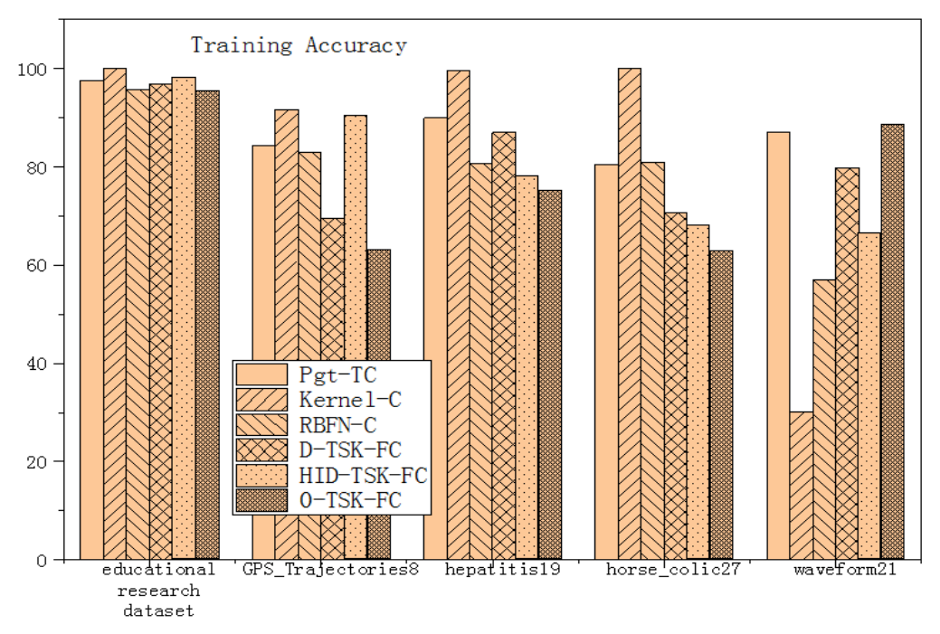
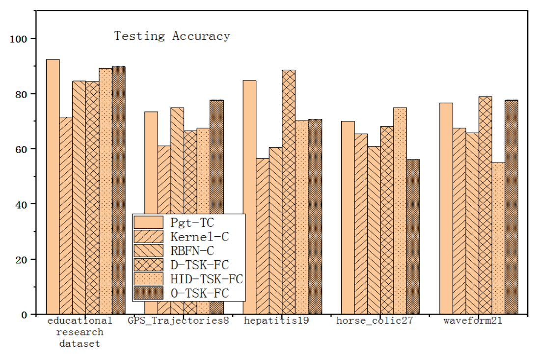
Based on Figure 2 and Figure 3, for the educational research dataset, although the non-fuzzy classifier Kernel-C achieved the highest top training accuracy, Pgt-TC’s top training accuracy is superior compared to other fuzzy classifiers. Furthermore, Pgt-TC ranks first in top testing accuracy among all compared algorithms. For the other four UCI datasets, the training accuracy of Pgt-TC also leads most classifiers. Although it did not achieve the top position on some datasets, it primarily lagged behind the non-fuzzy classifier Kernel-C. It is noteworthy that the Kernel-C algorithm is an unexplainable “black-box” algorithm. In terms of top testing accuracy, Pgt-TC still outperforms the majority of classifiers and demonstrates relatively stable performance, with rare instances of testing accuracy being significantly lower than training accuracy, indicating excellent generalization capability.

To further evaluate the stability and reliability of the experimental results, each method was independently run five times under the same experimental settings. The mean testing accuracy and standard deviation were calculated and reported in

Table 4. Statistical results of testing accuracy over five independent runs (%).

Dataset	Pgt-TC	Kernel-C	RBFS-C	D-TSK-FC	HTD-TSK-FC	O-TSK-FC
Educational research dataset	92.36 ± 0.61	71.48 ± 1.35	84.72 ± 0.92	84.31 ± 0.97	88.76 ± 0.74	89.53 ± 0.68
GPS trajectories	73.42 ± 1.18	61.36 ± 1.64	74.58 ± 1.09	66.71 ± 1.43	67.52 ± 1.37	77.38 ± 1.02
Hepatitis	84.67 ± 0.88	56.83 ± 1.72	60.74 ± 1.55	88.61 ± 0.76	70.45 ± 1.28	70.62 ± 1.31
Horse colic	70.18 ± 1.22	65.47 ± 1.41	61.35 ± 1.66	68.42 ± 1.34	74.63 ± 1.07	55.86 ± 1.83
Waveform	76.58 ± 1.04	67.36 ± 1.39	65.82 ± 1.45	78.52 ± 0.96	55.27 ± 1.89	77.41 ± 1.01

. Compared with only reporting a single accuracy value, the use of mean accuracy and standard deviation can more clearly reflect the average performance and fluctuation of different methods.

As shown in

Table 5. Overall statistical comparison of testing accuracy (%).

Method	Average Testing Accuracy	Average Standard Deviation	Average Rank
Pgt-TC	79.44	0.99	2.2
Kernel-C	64.5	1.5	5.2
RBFS-C	69.44	1.33	4.2
D-TSK-FC	77.31	1.09	3
HTD-TSK-FC	71.33	1.27	3.6
O-TSK-FC	74.16	1.17	2.8

, the proposed Pgt-TC model achieves the highest average testing accuracy among all comparison methods. Although Pgt-TC does not obtain the best result on every dataset, it shows competitive performance across different datasets and maintains the smallest average standard deviation. This indicates that the proposed method has good robustness and stable generalization ability. In addition, the average rank of Pgt-TC is also the best among all methods, which further demonstrates the overall effectiveness of the proposed model.

3.2.2. Comparison of SE Values

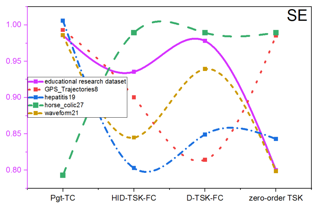
This subsection discusses the average SE values of the four fuzzy classifiers across the five datasets. In the context of research on teaching process intervention, taking the educational research dataset as an example, the SE value reflects the model’s effectiveness in identifying students requiring instructional intervention. As shown in Figure 4, Pgt-TC achieves an average SE value of 98.60, ranking highest among all fuzzy classifiers.

3.3. Parameter Sensitivity Study

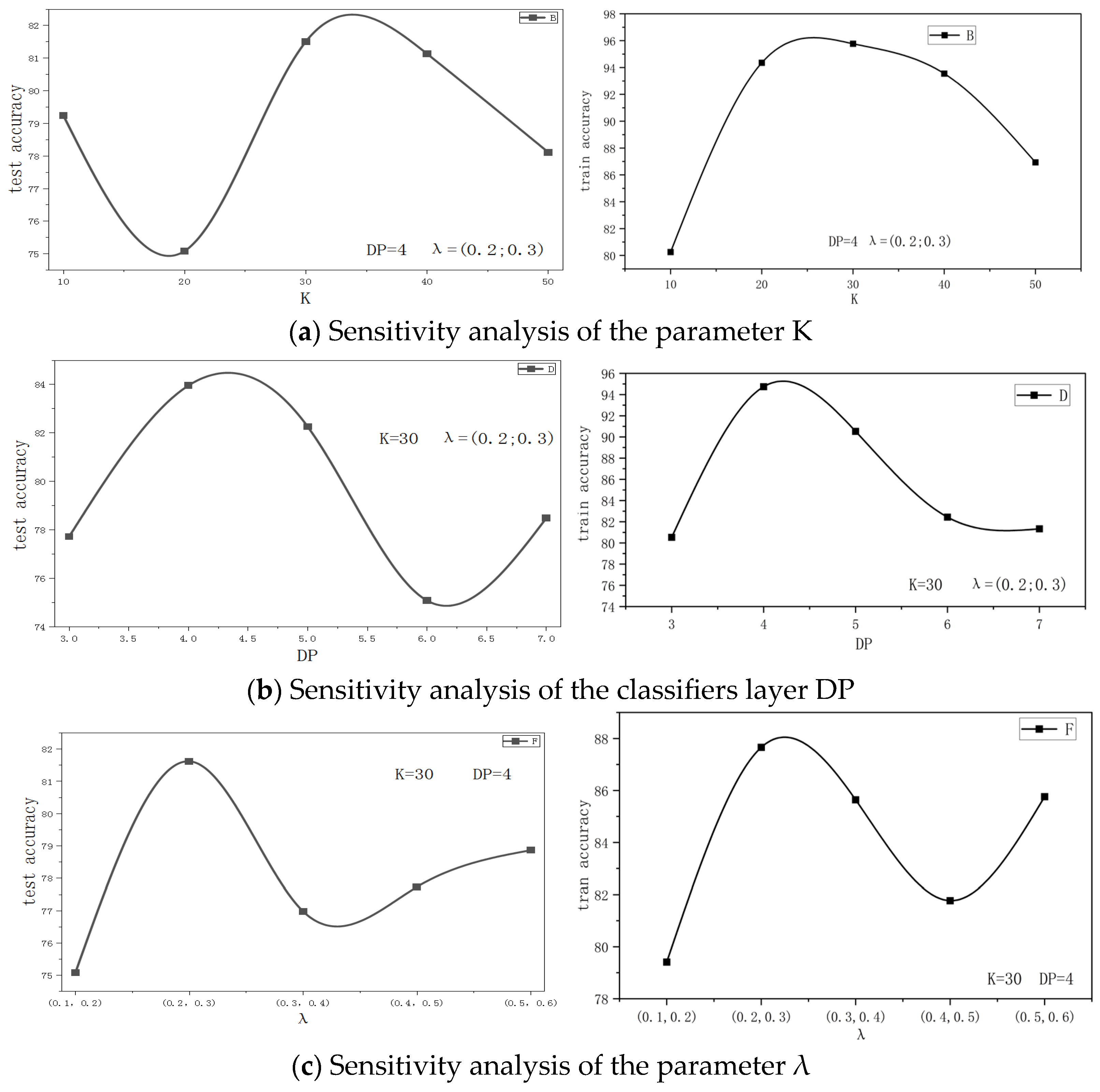
Clearly, the number of fuzzy rules K, the depth of the model DP, and the disturbance parameter $\lambda$ all have an impact on the experimental results. Therefore, in this section, using the educational research dataset as an example, each experiment was independently repeated five times under the same experimental settings, and the mean test accuracy and standard deviation were reported to evaluate both the average performance and stability of the model.

According to Figure 5a, when the number of fuzzy rules is below 30, Pgt-TC is relatively sensitive to this parameter. When the number of fuzzy rules exceeds 30, the improvement in the best test accuracy becomes less significant. Moreover, when the total number of fuzzy rules far exceeds 30, overfitting may occur, leading to a decline in test accuracy. Considering that too many fuzzy rules can reduce the model’s interpretability, while too few rules may oversimplify the model, this study sets the number of fuzzy rules (K) to 30. The training accuracy also reaches a relatively high level around K = 30, indicating that this setting can maintain sufficient fitting ability on the training set while avoiding excessive rule complexity.

According to Figure 5b, the test accuracy shows an initial increase followed by a decrease as the training depth increases. In other words, when the training depth becomes too large, Pgt-TC exhibits overfitting. Therefore, after comprehensive consideration, the training depth (dp) is set to 4. From the training accuracy curve, DP = 4 also achieves the best fitting performance on the training set, which further supports the rationality of selecting this depth.

Figure 5c illustrates the impact of the two disturbance parameters (λ) on the test accuracy. To determine the optimal values for these parameters, this study employed a grid search method with a step size of 0.1. It can be observed that the test accuracy reaches its peak when the values of the two λ parameters are set to (0.2, 0.3). The training accuracy under this parameter combination is also relatively high, suggesting that λ = (0.2, 0.3) provides a better balance between training-set fitting and test-set generalization.

3.4. Nonparametric Statistical Analysis

This study conducted a Friedman test [29] on the best test accuracy achieved by the six algorithms across the five datasets to evaluate whether there were significant differences among them. According to

Table 6. Average rankings of the algorithms.

Algorithm	Ranking	p-Value
Kernel-C	2.6	0.118536
RBFN-C	3.6
D-TSK-FC	4
HID-TSK-FC	4.2
0-order TSK	4.8
Pgt-TC	1.8

, the average rankings of the six algorithms is the first.

To further examine pairwise differences among the algorithms, a post hoc Holm test was performed. The null hypothesis assumes that there is no significant performance difference between the proposed method and each compared algorithm. A p-value less than or equal to 0.05 indicates a statistically significant difference, allowing us to reject the null hypothesis. As shown in

Table 7. Post hoc comparison table for α = 0.05.

i	Algorithm	z = (R0 − Ri)/SE	p	Holm = α/i	Null Hypothesis
5	0-order TSK-FC fuzzy classifier	2.535463	0.01123	0.01	Reject
4	HID-TSK-FC	2.02837	0.042522	0.0125	Reject
3	D-TSK-FC	1.859339	0.062979	0.016667	Not Reject
2	RBFN-C	1.521278	0.12819	0.025	Not Reject
1	Kernel-C	0.676123	0.498962	0.05	Not Reject

, although the null hypotheses for Kernel-C, RBFN-C, and D-TSK-FC are not rejected, the experimental results in Section 3.2 demonstrate that the proposed method still achieves superior or comparable average performance across all datasets. Moreover, Kernel-C and RBFN-C are black-box models with limited interpretability. Although D-TSK-FC is more interpretable due to its fuzzy-rule-based structure, it relies on stochastic mechanisms in feature selection, rule generation, and hierarchical construction, which may lead to performance fluctuations and reduced stability. In contrast, the proposed method achieves competitive performance while offering a more stable and interpretable modeling process, making it suitable for tasks requiring both accuracy and transparency.

3.5. Semantic Interpretability Analysis

The semantic interpretability of the proposed Pgt-TC model is crucial for assisting educational institutions in implementing targeted teaching interventions for students. Using the educational research dataset as an example, this section explains the logical interpretation of each fuzzy rule.

Table 8. Antecedent and Consequent Parameters of the six rules and Gaussian Membership Function.

	#	Rule 1	Rule 2	Rule 3	Rule 4	Rule 5	Rule 6
F1	$e^{-\frac{1}{2}{\left(\frac{x-c_1^k}{{\sigma }_1^k}\right)}^2}$	$e^{-\frac{1}{2}{\left(\frac{x-0}{1}\right)}^2}$	$e^{-\frac{1}{2}{\left(\frac{x-0.9234}{0.9873}\right)}^2}$	$e^{-\frac{1}{2}{\left(\frac{x-1}{0.9923}\right)}^2}$	$e^{-\frac{1}{2}{\left(\frac{x-0.6157}{0.9443}\right)}^2}$	$e^{-\frac{1}{2}{\left(\frac{x-0}{1}\right)}^2}$	$e^{-\frac{1}{2}{\left(\frac{x-0}{1}\right)}^2}$
F2	$e^{-\frac{1}{2}{\left(\frac{x-c_2^k}{{\sigma }_2^k}\right)}^2}$	$e^{-\frac{1}{2}{\left(\frac{x-0.0289}{0.9918}\right)}^2}$	$e^{-\frac{1}{2}{\left(\frac{x-1}{0.9901}\right)}^2}$	$e^{-\frac{1}{2}{\left(\frac{x-0.7004}{0.9478}\right)}^2}$	$e^{-\frac{1}{2}{\left(\frac{x-0.2312}{0.9414}\right)}^2}$	$e^{-\frac{1}{2}{\left(\frac{x-0.2649}{0.9245}\right)}^2}$	$e^{-\frac{1}{2}{\left(\frac{x-1}{0.9651}\right)}^2}$
F3	$e^{-\frac{1}{2}{\left(\frac{x-c_3^k}{{\sigma }_3^k}\right)}^2}$	$e^{-\frac{1}{2}{\left(\frac{x-1}{0.9828}\right)}^2}$	$e^{-\frac{1}{2}{\left(\frac{x-0.2619}{0.9867}\right)}^2}$	$e^{-\frac{1}{2}{\left(\frac{x-0.0219}{0.9938}\right)}^2}$	$e^{-\frac{1}{2}{\left(\frac{x-0.1451}{0.9496}\right)}^2}$	$e^{-\frac{1}{2}{\left(\frac{x-0.8589}{0.9139}\right)}^2}$	$e^{-\frac{1}{2}{\left(\frac{x-0.4309}{0.9280}\right)}^2}$
F4	$e^{-\frac{1}{2}{\left(\frac{x-c_4^k}{{\sigma }_4^k}\right)}^2}$	$e^{-\frac{1}{2}{\left(\frac{x-0.8503}{0.9601}\right)}^2}$	$e^{-\frac{1}{2}{\left(\frac{x-0}{1}\right)}^2}$	$e^{-\frac{1}{2}{\left(\frac{x-0.6940}{0.9473}\right)}^2}$	$e^{-\frac{1}{2}{\left(\frac{x-1}{1}\right)}^2}$	$e^{-\frac{1}{2}{\left(\frac{x-1}{0.9336}\right)}^2}$	$e^{-\frac{1}{2}{\left(\frac{x-0.2212}{0.9052}\right)}^2}$
F5	$e^{-\frac{1}{2}{\left(\frac{x-c_5^k}{{\sigma }_5^k}\right)}^2}$	$e^{-\frac{1}{2}{\left(\frac{x-0.6746}{0.9501}\right)}^2}$	$e^{-\frac{1}{2}{\left(\frac{x-0.6918}{0.9822}\right)}^2}$	$e^{-\frac{1}{2}{\left(\frac{x-0}{1}\right)}^2}$	$e^{-\frac{1}{2}{\left(\frac{x-0}{0.9733}\right)}^2}$	$e^{-\frac{1}{2}{\left(\frac{x-0.7102}{0.9014}\right)}^2}$	$e^{-\frac{1}{2}{\left(\frac{x-0.9960}{0.9644}\right)}^2}$
$\cdots$		$\cdots$	$\cdots$	$\cdots$	$\cdots$	$\cdots$	$\cdots$
	p	0.6775	0.5747	0.8395	0.6214	0.9140	0.7081

provides explanations for six representative rules from the dataset.

In this study, the cluster centers c were normalized to fall within the interval [0, 1]. Corresponding logical interpretations were assigned to these cluster centers by dividing the interval into five equal segments: (0.0–0.2], (0.2–0.4], (0.4–0.6], (0.6–0.8], and (0.8–1.0]. These segments correspond to the linguistic labels Very Low, Low, Medium, High, and Very High, respectively. Each cluster center receives an interpretation based on the specific sub-interval in which its value lies.

Each rule should be concise and straightforward, which facilitates the application of the model in the field of blended learning intervention research and enhances interpretability. Taking the “IF-THEN” form of the first rule as an example:

IF       Prerequisite Course 1 is very low
               Prerequisite Course 2 is very low
                 Prerequisite Course 3 is very high
                               the number of videos watched is very high
                       the number of videos watched is high
               …   …
THEN      f¹(x) = 0.6775                                  

4. Conclusions

This study addresses challenges in educational intervention by introducing a hierarchical TSK fuzzy classifier, leveraging its high performance and strong interpretability to provide teachers with more accurate instructional recommendations.

A novel rule generation method was proposed to filter important rules and propagate them to subsequent basic building units, ensuring overall model performance. Two input subspaces were established based on identical samples but different feature dimensions to validate the effectiveness of newly added features for teaching intervention.

A new output weight optimization mechanism was introduced to reduce approximation errors between different basic building units, thereby enhancing model consistency and interpretability. Through a stacked structure and quasi-stacked architecture, the model’s generalization capability and consistency were ensured, leading to improved classifier performance.

Experimental results demonstrate that Pgt-TC exhibits strong classification performance and interpretability in monitoring the actual teaching process and evaluation of teaching effectiveness.

This study also has some unresolved issues: (1) Pgt-TC identifies students needing intervention and provides feature-level diagnostic information, but does not prescribe specific intervention strategies. Translating diagnostics into concrete teaching actions remains the teacher’s responsibility. Future work could integrate Pgt-TC’s diagnostic capability with an intervention strategy recommendation module. (2) Pgt-TC is currently evaluated only in an offline experimental setting. Its usability, acceptance, and effectiveness in real educational environments—where teachers use rule-based explanations to make decisions—have not been assessed. User studies involving teachers and administrators would offer valuable insights into its practical utility.

References

1. UNESCO. Global Education Monitoring Report 2024: Technology in Education—A Tool on Whose Terms? UNESCO: Paris, France, 2024. [Google Scholar]
2. Boeskens, L.; Meyer, K. Policies for the Digital Transformation of School Education: Evidence from the Policy Survey on School Education in the Digital Age; OECD Education Working Papers, No. 328; OECD Publishing: Paris, France, 2025. [Google Scholar] [CrossRef]
3. Ministry of Education of the People’s Republic of China. China Smart Education Development Report (2024–2025); Educational Science Publishing House: Beijing, China, 2025.
4. Chen, L.; Wang, W.; Li, P. Research on digital educational resource evaluation and standard development. E-Educ. Res. 2013, 34, 61–66. (In Chinese) [Google Scholar]
5. Yin, H.; Yu, Z.; Yi, Q. Construction of an evaluation index system for smart classrooms. Mod. Educ. Technol. 2020, 30, 80–87. (In Chinese) [Google Scholar]
6. Baker, R.S.; Siemens, G. Educational data mining and learning analytics. In Encyclopedia of the Sciences of Learning; Springer: New York, NY, USA, 2014; pp. 1–4. [Google Scholar] [CrossRef]
7. Chen, L.; Ren, P.; Zhang, W. Post-pandemic era educational innovation: New horizons and China’s exemplary explorations—Reflections on attending the 2020 Global Artificial Intelligence and Education Big Data Conference. China Educ. Technol. 2021, 5, 1–9. (In Chinese) [Google Scholar] [CrossRef]
8. Hattie, J. Visible Learning: A Synthesis of over 800 Meta-Analyses Relating to Achievement; Routledge: Abingdon, UK, 2017. [Google Scholar]
9. Zhang, Y.; Wang, Q.; Li, H. An empirical study on the effect of intelligent teaching intervention. J. Distance Educ. 2022, 40, 45–54. (In Chinese) [Google Scholar]
10. Hu, Y.; Duan, L. Decision Support Framework for Digital Music Integration in Education Reform Using Picture Fuzzy FUCA and Industry–Academia Collaboration. Symmetry 2026, 18, 145. [Google Scholar] [CrossRef]
11. Rojas, J.A.; Espitia, H.E.; Bejarano, L.A. Design and Optimization of a Fuzzy Logic System for Academic Performance Prediction. Symmetry 2021, 13, 133. [Google Scholar] [CrossRef]
12. Jaukovic Jocic, K.; Jocic, G.; Karabasevic, D.; Popovic, G.; Stanujkic, D.; Zavadskas, E.K.; Thanh Nguyen, P. A Novel Integrated PIPRECIA–Interval-Valued Triangular Fuzzy ARAS Model: E-Learning Course Selection. Symmetry 2020, 12, 928. [Google Scholar] [CrossRef]
13. Albaity, M.; Mahmood, T.; Ali, Z. Analysis and Applications of Artificial Intelligence in Digital Education Based on Complex Fuzzy Clustering Algorithms. Mathematics 2023, 11, 3184. [Google Scholar] [CrossRef]
14. Maitra, S.; Madan, S.; Mahajan, P. An Adaptive Neural Fuzzy Inference System for prediction of student performance in Higher Education. In Proceedings of the 2018 International Conference on Advances in Computing, Communication Control and Net-working (ICACCCN), Greater Noida, India, 12–13 October 2018; pp. 1158–1163. [Google Scholar] [CrossRef]
15. de Jesus, C.G.; Ledda, M.K.C. Intervention Support Program for Students at Risk of Dropping Out Using Fuzzy Logic-Based Prescriptive Analytics. In Proceedings of the 2021 IEEE 17th International Colloquium on Signal Processing & Its Applications (CSPA), Langkawi, Malaysia, 5–6 March 2021; pp. 160–165. [Google Scholar] [CrossRef]
16. Zhou, T.; Chung, F.-L.; Wang, S. Deep TSK Fuzzy Classifier With Stacked Generalization and Triplely Concise Interpretability Guarantee for Large Data. IEEE Trans. Fuzzy Syst. 2017, 25, 1207–1221. [Google Scholar]
17. Xie, R.; Wang, S. A wide interpretable Gaussian Takagi–Sugeno–Kang fuzzy classifier and its incremental learning. Knowl.-Based Syst. 2022, 241, 108203. [Google Scholar] [CrossRef]
18. Takagi, T.; Sugeno, M. Fuzzy identification of systems and its application to modeling and control. IEEE Trans. Syst. Man Cybern. 1985, 15, 116–132. [Google Scholar] [CrossRef]
19. Deng, Z.; Cao, L.; Jiang, Y.; Wang, S. Minimax probability TSK fuzzy system classifier: A more transparent and highly interpretable classification model. IEEE Trans. Fuzzy Syst. 2015, 23, 813–826. [Google Scholar]
20. Azam, M.H.; Hasan, M.H.; Hassan, S.; Abdulkadir, S.J. Fuzzy Type-1 Triangular Membership Function Approximation Using Fuzzy C-Means. In Proceedings of the 2020 International Conference on Computational Intelligence, Bandar Seri Iskandar, Malaysia, 8–9 October 2020; pp. 115–120. [Google Scholar]
21. Murata, T.; Ishibuchi, H. Adjusting membership functions of fuzzy classification rules by genetic algorithms. In Proceedings of the 1995 IEEE International Conference on Fuzzy Systems, Yokohama, Japan, 20–24 March 1995; Volume 4, pp. 1819–1824. [Google Scholar]
22. Benitez-Diaz, D.; Garcia-Quesada, J. Learning algorithm with Gaussian membership function for Fuzzy RBF neural networks. In Proceedings of the International Workshop on Artificial Neural Networks, Malaga-Torremolinos, Spain, 7–9 June 1995; pp. 527–534. [Google Scholar]
23. Bezdek, J.C.; Ehrlich, R.; Full, W.E. FCM: The fuzzy c-means clustering algorithm. Comput. Geosci. 1984, 10, 191–203. [Google Scholar] [CrossRef]
24. Bayindir, R.; Gok, M.; Kabalci, E.; Kaplan, O. An intelligent power factor correction approach based on linear regression and ridge regression methods. In Proceedings of the 2011 10th International Conference on Machine Learning and Applications and Workshops, Honolulu, HI, USA, 18–21 December 2011; pp. 313–315. [Google Scholar]
25. Deng, Z.; Choi, K.; Jiang, Y.; Wang, S. Generalized hidden-mapping ridge regression, knowledge-leveraged inductive transfer learning for neural networks, fuzzy systems and kernel methods. IEEE Trans. Cybern. 2014, 44, 2585–2599. [Google Scholar] [PubMed]
26. Zhou, T.; Zhou, Y.; Gao, S. Quantitative-integration-based TSK fuzzy classification through improving the consistency of multi-hierarchical structure. Appl. Soft Comput. 2021, 106, 107350. [Google Scholar]
27. Zhang, Y.; Ishibuchi, H.; Wang, S. Deep Takagi–Sugeno–Kang Fuzzy Classifier With Shared Linguistic Fuzzy Rules. IEEE Trans. Fuzzy Syst. 2018, 26, 1535–1549. [Google Scholar]
28. Alcalá-Fdez, J.; Fernández, A.; Luengo, J.; Derrac, J.; García, S.; Sánchez, L.; Herrera, F. Keel data-mining software tool: Data set repository, integration of algorithms and experimental analysis framework. J. Mult.-Valued Log. Soft Comput. 2011, 17, 255–287. [Google Scholar]
29. Demsar, J. Statistical comparisons of classifiers over multiple data sets. J. Mach. Learn. Res. 2006, 7, 1–30. [Google Scholar]
Figure 1. Model Figure.
Symmetry 18 01137 g001
Figure 2. Comparison of Training Accuracies of Six Classifiers on Five Datasets.
Symmetry 18 01137 g002
Figure 3. Comparison of Testing Accuracies of Six classifiers on Five Datasets.
Symmetry 18 01137 g003
Figure 4. Comparison of SE Values for Six Algorithms.
Symmetry 18 01137 g004
Figure 5. Comparison of Parameter Sensitivity.
Symmetry 18 01137 g005