Article

Dual-Domain Symmetry: A Frequency-Aware Residual U-Net for High-Fidelity EEG Artifact Removal

1
School of Mechanical and Electrical Engineering, Chengdu University of Technology, Chengdu 610059, China
2
School of Computer and Network Security, Chengdu University of Technology, Chengdu 610059, China
*
Author to whom correspondence should be addressed.
Symmetry 2026, 18(6), 988; https://doi.org/10.3390/sym18060988
Submission received: 23 April 2026 / Revised: 30 May 2026 / Accepted: 5 June 2026 / Published: 8 June 2026

Abstract

Electroencephalography (EEG) is a non-invasive technique used to monitor brain activity but is prone to physiological artifacts, especially eye movements (EOG) and muscle contractions (EMG). These artifacts are non-stationary and frequently overlap with neural oscillation bands, making them difficult to separate accurately from genuine EEG activity. Conventional single-domain filters often fail to eliminate such interference, resulting in either residual noise or the unintended suppression of authentic EEG data. To address these limitations, we propose a Frequency-Aware Residual U-Net (FARU-Net), a dual-domain, frequency-aware residual architecture for EEG artifact removal designed to improve restoration fidelity. Unlike models based solely on temporal features, FARU-Net explicitly modulates the spectral properties of the signal in the latent space through a Frequency-aware Bottleneck Module (FBM), while simultaneously refining temporal details. Additionally, Attention Gates (AGs) are integrated into the skip connections to refine feature fusion and reduce residual noise while preserving salient waveform structures. Comparative experiments on the EEGdenoiseNet benchmark demonstrate that FARU-Net achieves strong overall performance for single-channel EEG restoration. Across five independent test groups, the proposed model attains a mean Pearson correlation coefficient (CC) of 0.9681 and a mean signal-to-noise ratio improvement (ΔSNR) of 26.66 dB. These results indicate that the proposed method effectively preserves both waveform morphology and spectral structure compared with conventional U-Net variants and CNN-based models.

1. Introduction

Electroencephalography (EEG) is a non-invasive technique for monitoring brain activity with high temporal resolution, making it valuable for applications such as brain-computer interfaces (BCIs) and clinical diagnostics [1]. Recent advances in wearable electronics have extended EEG monitoring from laboratory-only use to daily life applications. Mobile health (mHealth) applications have enabled out-of-clinic EEG monitoring through portable single-channel sensors. However, because these devices use a single-channel design and lack spatial redundancy, the acquired signals are highly susceptible to interference. Consequently, physiological artifacts such as eye movements (EOG) and muscle contractions (EMG) can interfere considerably with the neural signals hiding significant brain rhythms (i.e., α , β , γ ) and decreasing the precision of further analysis [2,3]. Despite advances in artifact removal techniques, a universal and robust solution remains elusive. Furthermore, research indicates that high-quality denoising can improve the performance of downstream EEG tasks [4].
Traditional techniques, such as Independent Component Analysis (ICA) and regression-based methods, have been widely used because they are relatively interpretable [1]. However, these methods often depend on strict statistical assumptions or require manual adjustments. Moreover, when the spectra of artifacts overlap with neural signals, linear decomposition can result in “over-denoising,” where crucial neural information is inadvertently removed. To address these shortcomings, deep learning (DL) has emerged as a promising data-driven approach for EEG restoration [3]. Furthermore, the architectural evolution from standard U-Nets to nested structures like UNet++ [5] has significantly enhanced feature fusion efficiency through dense skip connections. Recent models, such as Convolutional Neural Networks (CNNs) [6] and U-Net-based architectures [7,8], have shown strong performance in capturing complex, non-linear relationships. Notably, the IC-U-Net [8] framework demonstrated the efficacy of using U-Net structures for sample-level EEG reconstruction by leveraging independent component mixtures. For single-channel EEG recordings, where spatial correlations are absent, dual-branch architectures [9] and Transformer-based models [10], as well as hybrid CNN–Transformer designs [11], have been explored to effectively separate clean neural signals from contaminants. Meanwhile, efficient networks such as EDGeNet [12] have been developed to enable fast and lightweight EEG denoising for real-time wearable applications.
Beyond the hardware constraints of portable devices, EEG artifact removal faces several intertwined challenges that span signal characteristics, algorithmic design, and deployment requirements. Physiological artifacts such as EOG and EMG are inherently non-stationary and exhibit substantial inter-subject variability [2,3], rendering static filtering or manual thresholding ineffective [1]. Moreover, the intrinsic spectral overlap between artifacts and neural oscillations (e.g., δ / θ rhythms with ocular activity, γ -band with myogenic bursts) fundamentally limits purely temporal optimization strategies, which often suffer from spectral blurring or unintended suppression of neurophysiological content [13]. Concurrently, the growing demand for real-time ambulatory monitoring imposes strict computational constraints, necessitating architectures that balance reconstruction fidelity with inference efficiency [12]. Finally, the absence of ground-truth clean EEG in real-world recordings complicates both model training and objective evaluation, highlighting the need for generalizable, dual-domain learning strategies that do not rely solely on synthetic data assumptions [4,14]. While single-channel designs intensify these challenges due to the lack of spatial redundancy, they collectively motivate the development of adaptive [15], frequency-aware frameworks capable of disentangling non-stationary interference from genuine neural dynamics [16,17]. To address this limitation, we propose FARU-Net, a frequency-aware residual U-Net architecture that jointly models temporal and spectral features. By incorporating explicit frequency-domain constraints into the learning process, the proposed framework aims to improve both waveform reconstruction accuracy and spectral fidelity.
Conventional deep learning filters often rely solely on time-domain supervision, such as Mean Squared Error (MSE). This approach can lead to the over-smoothing of high-frequency neural rhythms, causing spectral blurring. To address this, we present a spectral–temporal joint optimization framework [18]. By explicitly applying frequency-domain magnitude constraints through the Frequency-aware Bottleneck Module (FBM), the proposed method prevents the loss of critical neurophysiological features [19]. Furthermore, this joint-domain approach is adaptable. This framework can also be integrated into existing time-domain denoising models as a regularization strategy, improving both morphological accuracy and spectral fidelity.
The main contributions of this work are as follows:
  • We propose FARU-Net, a residual encoder–decoder architecture designed for high-fidelity EEG signal restoration.
  • A Frequency-aware Bottleneck Module (FBM) is introduced to perform spectral recalibration in the latent space, enabling adaptive emphasis on task-relevant neural rhythms.
  • Attention Gates (AGs) are incorporated into skip connections to refine feature fusion and suppress irrelevant components.
  • A spectral–temporal joint loss function is developed to preserve both waveform morphology and frequency-domain characteristics.
The structure of this paper is organized as follows: Section 2 provides an overview of the existing EEG denoising literature, setting the theoretical context [1,2]. Section 3 presents the mathematical formulation of the FARU-Net architecture and the hybrid loss function. The proposed method is thoroughly evaluated through comparative experiments in Section 4, with Section 5 concluding with a discussion on future research directions [20].

2. Related Work

2.1. Traditional EEG Artifact Removal

Standard EEG artifact removal often relies on classical signal processing, such as regression-based methods, Independent Component Analysis (ICA), and wavelet transforms [1]. ICA decomposes multichannel EEG signals into statistically independent components to isolate artifacts, while wavelet-based methods adjust coefficients across multiple scales [21]. Although these approaches are interpretable, they typically require specific statistical assumptions or manual parameter selection [2]. Furthermore, when artifact spectra overlap with neural oscillations, linear decomposition can lead to the loss of neural information, affecting signal fidelity.

2.2. Deep Learning-Based EEG Denoising

The EEGdenoiseNet benchmark [14] has facilitated the development of data-driven methods for EEG restoration [3]. These approaches encompass various paradigms, including Fully Convolutional Neural Networks (FCNN), Recurrent Neural Networks (RNN), and specialized Convolutional Neural Network (CNN) topologies. For instance, 1D-ResCNN architectures utilize skip connections and residual learning to extract features from myogenic artifacts [22,23]. Furthermore, CNN-based approaches have been successfully applied to simultaneously remove concurrent EOG and EMG artifacts that frequently contaminate real-world EEG recordings [6]. To provide a theoretical framework for these diverse developments, a recent systematic exploration by Rakhmatulin et al. [24] categorized EEG feature extraction models into four primary archetypes: Standard, Recurrent, Decoder, and Combined architectures [25]. Crucially, they highlighted that decoder-based structures are particularly advantageous for high-fidelity signal reconstruction tasks, such as denoising.
U-Net-style architectures have been widely explored for EEG artifact removal due to their strong signal reconstruction ability. The residual U-Net paradigm has also demonstrated strong reconstruction capability in cross-domain tasks such as remote sensing road extraction [26], further validating its architectural generality for 1D signal restoration. CleanEEG employs a standard U-Net framework to achieve robust suppression of clinical artifacts while preserving critical epileptiform and oscillatory features [27]. On this basis, U-Net-style architectures, such as IC-U-Net [8], have been applied to achieve multi-scale signal restoration. Building upon this, Chang et al. [28] proposed an enhanced variant of IC-U-Net by incorporating nested dense skip connections to bridge the semantic gap between encoder and decoder features. This architectural refinement allows for higher feature reuse efficiency, achieving superior denoising performance with only half the parameter count of the original IC-U-Net. The landscape of deep learning has been further reshaped by the introduction of attention mechanisms, notably the Transformer architecture [29], which utilizes self-attention to capture long-range dependencies. Inspired by this paradigm shift, the integration of Attention Gates (AGs) [30] aims to enhance feature transfer between layers by focusing on specific regions of interest. AGs, originally developed for medical image segmentation [31], are used in FARU-Net to manage the feature fusion process within skip connections. Other developments involve specialized models for ocular artifact suppression [13] and hybrid architectures for non-stationary EEG signals, such as CNN-LSTM [32] and dual-pathway networks [33].

2.3. Design Rationale of FARU-Net

A variety of EEG artifact removal strategies have been developed for BCI applications [34]. However, current EEG denoising models often emphasize time-domain processing, which can limit their effectiveness in complex spectral environments. FARU-Net addresses these conditions through a dual-domain recalibration strategy. Advances in sequential signal processing have also demonstrated the effectiveness of joint time-frequency modeling for noise robust representation learning [16,35]. In contrast to dual-branch architectures [9,11], FARU-Net utilizes a single-branch symmetric structure with a Frequency-aware Bottleneck Module (FBM) to achieve spectral awareness. This architectural choice is informed by the success of adaptive gating mechanisms [36], which demonstrate that embedding multi-level context gating into encoder–decoder frameworks can significantly refine feature representation by weighting inter-dependencies between feature channels.
The FBM implements spectral recalibration at a reduced scale: by performing the Real-valued Discrete Fourier Transform (R-DFT) on latent features downsampled to 1 / 16 of their original length, the module captures global spectral dependencies with lower computational requirements compared to full-scale transforms. This allows the model to differentiate rhythms (e.g., 40 Hz Gamma oscillations) from broadband EMG noise that may be less distinguishable to purely temporal filters. By applying a joint loss function with a normalized magnitude constraint, FARU-Net aims to maintain spectral consistency, addressing the potential for spectral blurring in models optimized solely through Mean Squared Error (MSE).

3. Methodology

3.1. Problem Formulation

Let x R L denote the clean EEG signal and a R L represent the physiological artifacts.The observed EEG signal y can be expressed as the sum of the clean signal and the artifacts:
y = x + a
The goal is to learn a non-linear mapping function f θ ( · ) that reconstructs the clean signal, x ^ = f θ ( y ) , by minimizing the difference between the reconstructed signal and the original clean signal x in both the time and frequency domains.

3.2. Overall Architecture of FARU-Net

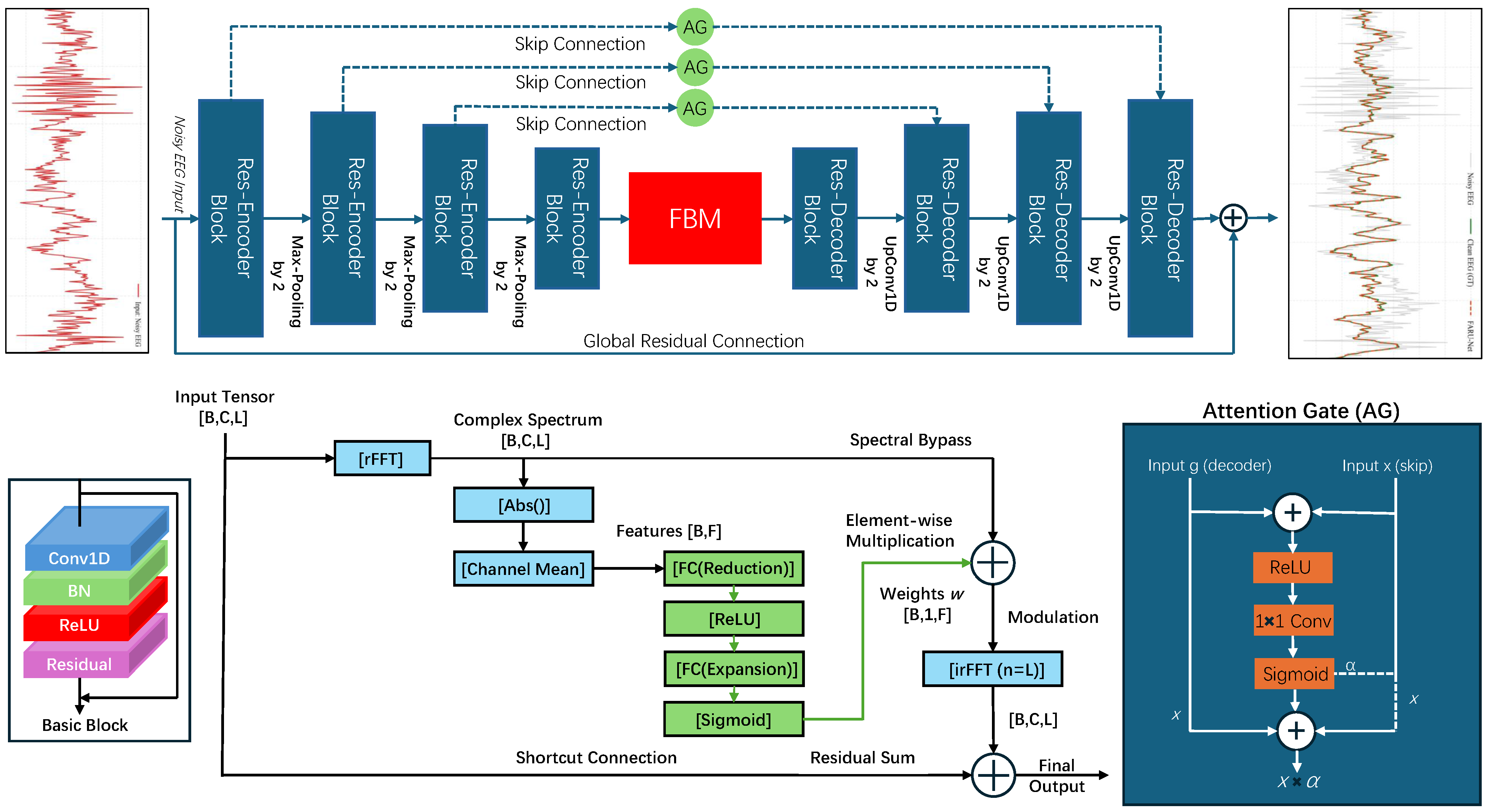
As illustrated in Figure 1, FARU-Net employs a symmetric encoder–decoder framework tailored for 1D physiological signal restoration. The backbone consists of stacked residual convolutional blocks that hierarchically extract multi-scale temporal features. To facilitate precise cross-scale information flow, each skip connection is augmented with an Attention Gate (AG), which dynamically modulates the relevance of skip features based on the decoder’s contextual signal before element-wise fusion. At the latent bottleneck, the network incorporates a Frequency-aware Bottleneck Module (FBM) to perform global spectral recalibration. Specifically, the FBM transforms intermediate features into the complex frequency domain via a real-valued FFT (rFFT), where a spectral bypass pathway and channel-wise modulation mechanism recalibrate rhythmic dependencies. This modulation is implemented through channel mean pooling, fully connected (FC) reduction/expansion layers, and a Sigmoid gating function. The recalibrated complex spectrum is then restored to the time domain via an inverse FFT (iFFT) and aggregated through a residual shortcut connection. By integrating local time-domain residual learning with this dual-domain recalibration strategy, FARU-Net effectively captures global rhythmic dependencies while adaptively refining multi-scale time-frequency features, enabling robust noise suppression without distorting critical physiological rhythms.

3.3. Frequency-Aware Bottleneck Module (FBM)

The FBM serves as the spectral core of the network, performing global spectral recalibration in the latent space. The specific symbolic flow of the dimension transformation within FBM is described as follows: Consider an intermediate feature map H R C × L at the deepest bottleneck (where L = L / 16 due to four successive downsampling stages). To generate a channel-independent spectral profile, we first apply global average pooling over the channel dimension to obtain h a v g = AvgPool C ( H ) R 1 × L . Strategically embedding this frequency-aware mechanism at the bottleneck enables the latent bottleneck to mitigate the receptive field constraints inherent in purely temporal convolutions. While 1D kernels extract local morphological patterns, they exhibit limited discriminative capacity for broadband EMG noise that overlaps with narrowband neural oscillations. By mapping latent features into the frequency domain via R-DFT at a compressed scale ( L / 16 ), the architecture implements global spectral recalibration, facilitating the frequency-selective prioritization of rhythms such as the 40 Hz Gamma oscillation.
We then perform the Real-valued Discrete Fourier Transform (R-DFT) on h a v g to obtain the magnitude spectrum M R 1 × ( L 2 + 1 ) . A learnable spectral weight vector w R 1 × ( L 2 + 1 ) is then computed via a two-layer structure:
w = σ W 2 · ReLU W 1 · M
where W 1 and W 2 are learnable parameters. The full spectral recalibration is achieved by applying the weights to the original latent spectrum: F ^ ( H ) = F ( H ) w , where ⊙ denotes frequency-wise multiplication. Finally, the signal is projected back to the time domain using the Inverse R-DFT:
H ^ = F 1 ( F ^ ( H ) ) + H
By processing downsampled features at the bottleneck, the computational complexity of the R-DFT is constrained to O ( L 16 log L 16 ) . This design ensures that the frequency-aware recalibration remains highly efficient compared to the O ( L · C 2 ) complexity of standard temporal convolutions.

3.4. Architectural Modules and Optimization Setup

The encoder and decoder stages are constructed using residual convolutional blocks, each comprising two sequential 1D convolutional layers ( k = 3 ) followed by batch normalization and ReLU activation. This design facilitates gradient flow and stabilizes training across deep layers. To bridge the semantic gap between encoder and decoder features, Attention Gates (AGs) are integrated into the skip connections. The AG utilizes an upsampled gating signal g to refine the encoder features x l by computing an attention coefficient α as:
q a t t = ψ T ReLU ( W g g + W x x l + b g ) + b ψ
α = σ ( BN ( q a t t ) )
This yields a refined feature map x ^ l = x l · α , which adaptively filters irrelevant components and ensures that only salient neural patterns are propagated to the decoder. To achieve high-fidelity EEG restoration, FARU-Net is optimized via a multi-objective framework that jointly constrains the model in both the time and frequency domains. First, we define the temporal loss L t i m e using Mean Squared Error (MSE) to minimize point-wise reconstruction errors:
L t i m e = 1 N i = 1 N x ^ i x i 2 2
Complementing this, we introduce a frequency-domain loss L f r e q that enforces spectral consistency by comparing normalized magnitude spectra:
L f r e q = E | F ( x ^ ) | mean ( | F ( x ^ ) | ) | F ( x ) | mean ( | F ( x ) | ) 1
Minimizing L f r e q encourages the network to preserve intrinsic rhythmic patterns while suppressing artifacts. These components are integrated into a unified objective function, weighted by the coefficient λ f :
L t o t a l = L t i m e + λ f L f r e q
This spectral–temporal joint optimization ensures that the model captures both the precise waveform morphology and the underlying spectral hierarchy of the EEG signals.
For training data generation, we adopt a linear additive contamination model aligned with the EEGdenoiseNetbenchmark [14]. Given a clean segment x ( t ) , composite artifacts a ( t ) are formed by randomly pairing EOG and EMG segments, yielding noisy observations y ( t ) = x ( t ) + λ · a ( t ) . The scaling factor λ is dynamically determined by a target SNR sampled uniformly from [ 7 , 2 ] dB, governed by the RMS power constraint:
λ = RMS ( x ) RMS ( a ) · 10 SNR 10
This synthesis protocol ensures that the simulated interference strictly adheres to established physiological characteristics and maintains consistency with prior comparative studies in the literature.

3.5. Evaluation Metrics

To quantitatively assess the reconstruction fidelity and generalization capability of the model, three primary evaluation metrics are employed. The relative root mean square error in the time domain ( R R M S E t i m e ) measures the overall morphological deviation between the denoised signal f ( y ) and the ground-truth x:
R R M S E t i m e = R M S ( f ( y ) x ) R M S ( x )
To evaluate spectral integrity, the relative root mean square error in the frequency domain ( R R M S E f r e q ) is calculated by comparing the power spectral density (PSD) of the signals:
R R M S E f r e q = R M S ( | F ( f ( y ) ) | | F ( x ) | ) R M S ( | F ( x ) | )
Furthermore, the Pearson correlation coefficient (CC) is utilized to determine the linear alignment and structural similarity between the reconstructed and clean EEG segments:
C C = C o v ( f ( y ) , x ) V a r ( f ( y ) ) V a r ( x )
Furthermore, to quantify the improvement in signal quality relative to the initial contamination level, we employ the Signal-to-Noise Ratio improvement (ΔSNR), defined as:
Δ SNR = SNRdenoised SNRnoisy
For R R M S E metrics, lower values represent higher reconstruction accuracy, while higher C C and Δ SNR values indicate superior waveform preservation and effective artifact suppression, respectively.

4. Experiments

4.1. Data Preparation and Preprocessing

The proposed FARU-Net was primarily evaluated using the EEGdenoiseNet benchmark, a large-scale dataset comprising 4514 clean EEG segments, 3400 EOG segments, and 5598 EMG segments. To ensure scientific rigor and prevent data leakage, a systematic processing protocol was implemented. Following the benchmark’s standard partition scheme, the raw segments were independently split into training, validation, and test sets with an 80:10:10 ratio. Specifically, the 4514 clean EEG segments were partitioned into 3611 training, 452 validation, and 451 test segments. The corresponding EOG and EMG artifact segments were segregated using an identical splitting strategy to guarantee that artifact morphologies encountered during training remained strictly absent from the evaluation phases. All segments were subsequently center-cropped or reflect-padded to a uniform length of 512 samples to ensure consistent temporal alignment across the pipeline.
To further verify the practical utility of the denoised signals in real-world brain-computer interface (BCI) applications, downstream classification experiments were conducted using the PhysioNet Motor Imagery dataset. EEG recordings from the first 30 subjects (S001–S030) were selected from runs 4, 8, and 12, which correspond to left- and right-hand motor imagery tasks. The original signals, sampled at 160 Hz, were preprocessed using a 1–40 Hz FIR bandpass filter to suppress baseline drift and high-frequency noise. Task-related epochs spanning 0 to 3.19375 s post-stimulus were extracted and uniformly resampled to 512 points to match the input dimensionality of FARU-Net. Finally, the event labels corresponding to left- and right-hand imagery (original codes 2 and 3) were mapped to binary labels (0 and 1) for classification evaluation.

4.2. Implementation Details

The detailed hardware configurations, software environment, and hyperparameter settings are summarized in Table 1. Following the EEGdenoiseNet protocol, we synthesized the dataset by linearly mixing clean EEG segments with EOG and EMG artifacts, yielding SNRs uniformly distributed between 7 dB and 2 dB [14]. All experiments were conducted on a workstation equipped with an NVIDIA RTX 4090 GPU (24 GB VRAM), an Intel Xeon Gold 6430 CPU, and 120 GB of RAM, running Ubuntu 22.04. The implementation leverages Python 3.12 and PyTorch 2.8.0 with CUDA 12.8.
For FARU-Net, optimization was performed using the Adam optimizer with an initial learning rate of 2.43 × 10 4 and a batch size of 128, trained over 150 epochs under a cosine annealing scheduler. To ensure a fair and rigorous comparison, the hyperparameters for all baseline models were similarly optimized using the Optuna framework with a TPE sampler. The resulting optimal configurations were: DAE1D (Adam, LR: 7.22 × 10 4 , Batch: 32), Complex CNN (Adam, LR: 8.25 × 10 4 , Batch: 64), and Simple CNN (Adam, LR: 9.09 × 10 4 , Batch: 32). Architecturally, FARU-Net employs a base channel width of 128 with a depth of 4. Each input segment spans 512 samples (corresponding to a 2 s window at 256 Hz), which are transformed via torch.fft.rfft into a 257-bin frequency representation, achieving a resolution of 0.5 Hz. The critical frequency-domain weight coefficient λ f was determined via the Optuna framework using a TPE sampler. Across 200 optimization trials, the optimal value was identified as 2.16 × 10 4 (Table 1), with subsequent ablation studies (Section 4.4) confirming it provides the ideal trade-off between artifact suppression and rhythmic preservation.

4.3. Comparison with Baseline Models

To provide a thorough evaluation of FARU-Net, we compare its performance with several representative baseline models, all trained and tested under the same setup. These include DAE1D, Complex CNN, Simple CNN, MultiRes-UNet3+, LinkNet, U-Net [7] and FPN. The comparison results are summarized in Table 2. While our primary evaluation focuses on a challenging signal-to-noise ratio (SNR) range of −7 dB to 2 dB to rigorously assess the model’s performance [14]. Further discussion of these results can be found in Section 5.
As detailed in Table 2, FARU-Net outperformed the compared models across the evaluated metrics, with the clearest advantage observed under high-noise conditions. At the 7 dB SNR level, FARU-Net yields a RRMSE time of 0.4753, which constitutes a reduction in error of approximately 57.9% relative to the Simple CNN (1.1286) and 47.5% relative to the Complex CNN (0.9056). Compared to the most competitive baseline at this intensity, MultiRes-UNet3+ (0.7830), the proposed architecture maintains a distinct performance margin with a 39.3% improvement in temporal reconstruction accuracy. Furthermore, the model yields a substantial SNR improvement, as evidenced by the performance trends in Table 2, where FARU-Net consistently suppresses mixed artifacts more effectively than the standard U-Net baseline (0.8122 for RRMSE time ) [7].
This degree of morphological preservation is attributed to the Frequency-aware Bottleneck Module (FBM), which facilitates the extraction of global spectral dependencies that temporal-only filters typically omit, thereby maintaining the integrity of neurophysiological oscillations. While FARU-Net achieves competitive performance, we conduct an incremental ablation study to better understand the contribution of each module.

4.4. Comparison with Recent Methods

In addition to the baseline model comparisons presented above, we further supplement comparisons with two EEG denoising models proposed in 2024–2025: EEGDiR [40] (Computers in Biology and Medicine) and TF-Denoiser [16] (Electronics). Both methods were originally designed for single-artifact removal (EOG-only or EMG-only). For fair comparison, we retrained FARU-Net under the same single-artifact protocol using the public EEGDenoiseNet dataset [14], with identical train/test splits and SNR ranges ( 7 to 2 dB). The quantitative results for EMG and EOG artifact removal are presented in Table 3 and Table 4, respectively.
Notably, while EEGDiR employs the Retentive Network for temporal modeling and TF-Denoiser uses joint time-frequency optimization with multi-attention mechanisms, FARU-Net’s single-path architecture with explicit spectral bottleneck yields consistently better reconstruction fidelity. This suggests that targeted frequency-domain regularization combined with temporal modeling may be more critical than pure temporal or naive time-frequency approaches for EEG denoising tasks.

4.5. Ablation Study

4.5.1. Impact of Architectural Components and Network Depth

To evaluate the contribution of each individual component in FARU-Net, we conducted an incremental ablation study. The results, averaged over five independent test groups, are summarized in Table 5. As shown in Table 5, starting from the baseline ResU-Net (a) [23], adding the Frequency-aware Bottleneck Module (b) yields the most significant performance improvement, underscoring the critical role of global spectral recalibration. Interestingly, integrating Attention Gates (AG) alone (Case c) causes a marginal CC drop (0.9682 to 0.9677), suggesting that without explicit spectral constraints, AGs may inadvertently suppress salient neural features amidst high-amplitude artifacts. However, introducing the spectral magnitude constraint L mag (Case d) fully realizes the synergy between global recalibration and local feature refinement, notably increasing ΔSNR from 26.40 dB (Case f) to 26.66 dB. This confirms that AGs act as fine-grained refiners only when operating under spectral supervision.
A key design choice in FARU-Net is the intentional omission of phase supervision in the loss function, distinguishing it from many existing dual-domain frameworks. This decision is rooted in the non-stationary nature of EEG signals; in single-channel scenarios, phase information is highly susceptible to stochastic artifacts and baseline drifts, making robust recovery exceptionally difficult. Our incremental ablation study in Table 5 justifies this strategy: the introduction of phase constraints (Setting e) failed to yield performance gains and even slightly degraded the CC and ΔSNR. This confirms that spectral magnitude serves as a more stable indicator for neural oscillation recovery than the volatile phase. Consequently, by prioritizing magnitude consistency, FARU-Net achieves superior restoration while maintaining computational efficiency for real-time applications.
Beyond modular components, the optimal network depth was rigorously determined through a dual-validation strategy. Manual ablation across depths of 2, 3, and 4 (Table 6) demonstrated that depth = 4 achieves peak reconstruction fidelity by optimally balancing receptive field expansion and feature preservation. This empirical finding was independently corroborated by the Optuna framework, which consistently identified depth = 4 as the global optimum across 200 independent trials.

4.5.2. Necessity of Time-Domain Supervision

To address whether frequency-domain supervision alone is sufficient for high-fidelity EEG reconstruction, we conducted a dedicated ablation study comparing three loss configurations: time-domain only ( L time ), frequency-domain only ( L freq ), and the proposed joint optimization. The quantitative results are summarized in Table 7. As shown in Table 7, relying solely on frequency-domain supervision leads to a severe degradation in amplitude-related metrics, despite maintaining a relatively high correlation coefficient. This phenomenon can be attributed to the scale ambiguity introduced by global magnitude normalization. While the normalized spectral loss effectively guides the model to learn the correct distribution of neural rhythms, it is mathematically invariant to absolute signal energy. Consequently, the model converges to a solution that matches the spectral shape but produces arbitrarily scaled outputs, resulting in catastrophic RRMSE and negative ΔSNR values.
This scale ambiguity is visually corroborated in Figure 2, which displays the time-domain waveforms reconstructed by the frequency-only model. As evident from the plots, although the model preserves the general oscillatory phase structure (consistent with the non-zero CC), the amplitude of the reconstructed signal diverges drastically from the ground truth, exhibiting severe scaling distortion. This qualitative evidence confirms that the reported quantitative degradation is intrinsic to the loss formulation rather than an artifact of training instability, and underscores why time-domain constraints are fundamentally necessary to anchor the absolute signal energy.
Conversely, the time-domain baseline successfully anchors the absolute amplitude and energy conservation, yet suffers from the well-documented “spectral blurring” effect, where high-frequency neural oscillations are unintentionally smoothed alongside artifacts. The proposed joint optimization elegantly resolves this trade-off: the time-domain MSE acts as a strict amplitude anchor, reducing scale ambiguity effectively, while the frequency-aware bottleneck retains fine-grained spectral characteristics. This synergistic mechanism confirms that time-domain constraints are not redundant but fundamentally necessary to ground the spectral learning process, enabling FARU-Net to achieve simultaneous temporal and spectral fidelity.

4.6. Qualitative Evaluation and Visualization

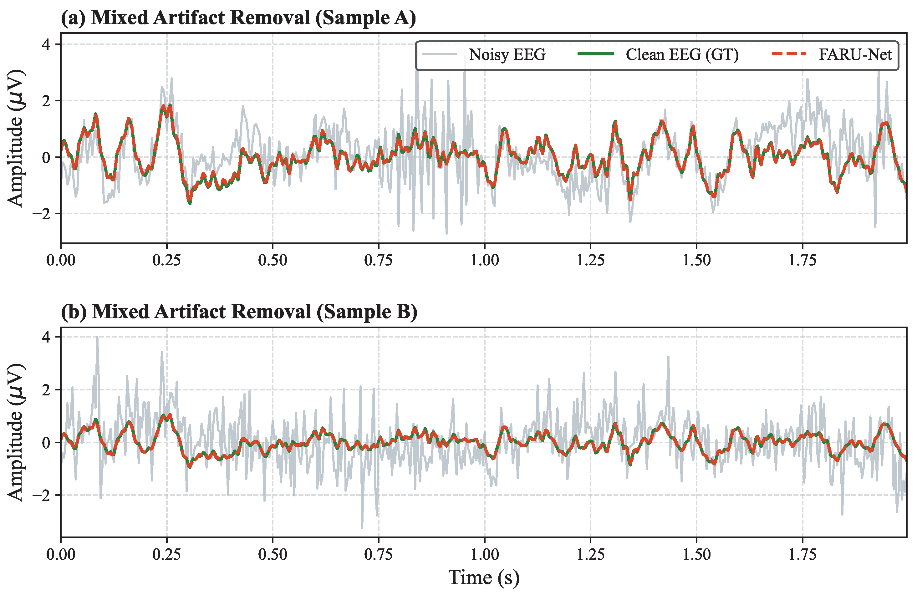
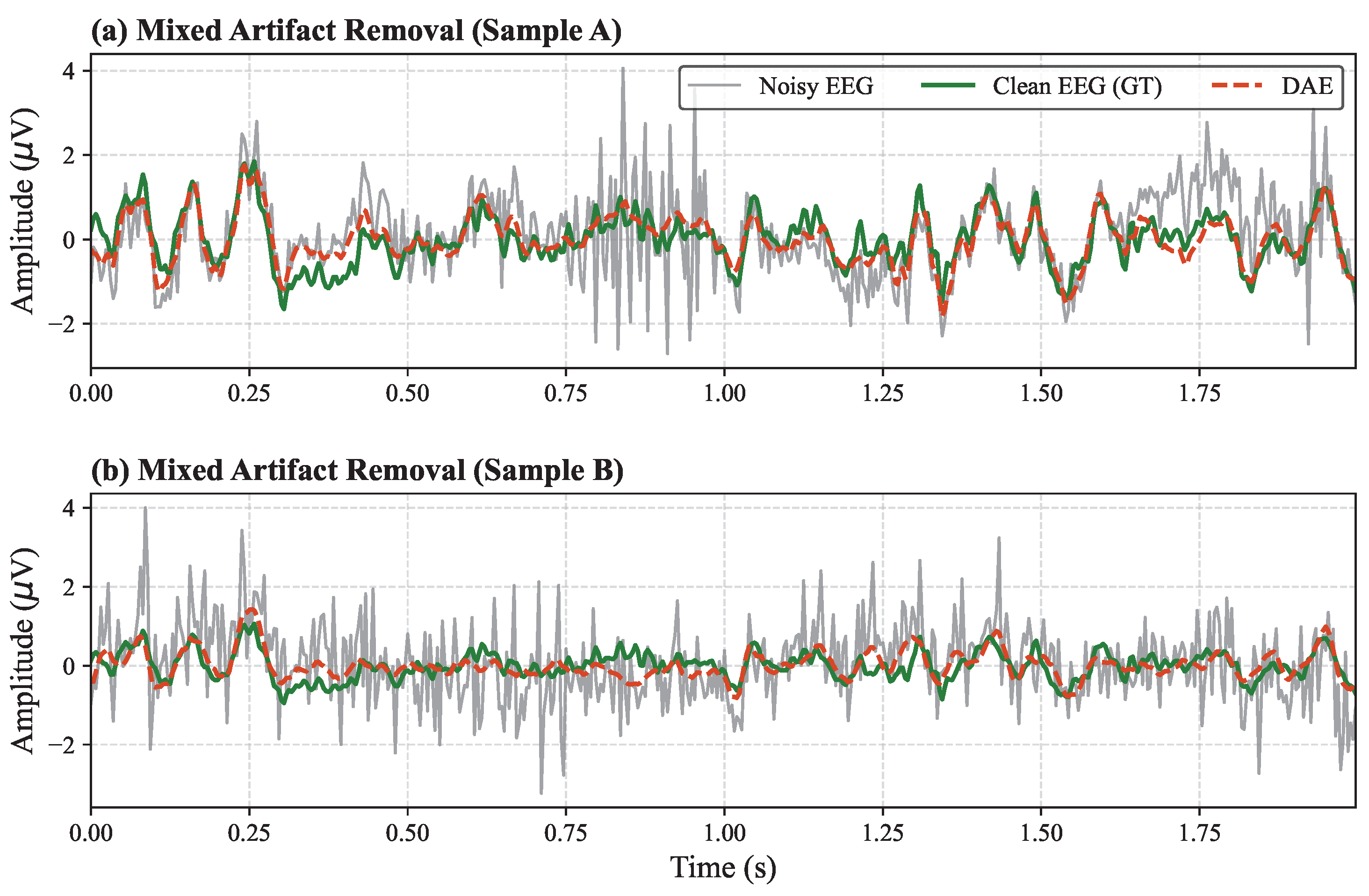
To better illustrate the denoising performance, we visualize both the temporal and spectral aspects of the reconstructed signals. Figure 3 shows the time-domain waveforms of two randomly selected EEG segments, each heavily corrupted by mixed physiological artifacts [14]. The noisy signals (solid grey lines) exhibit large amplitude fluctuations and high-frequency spikes that obscure the underlying neural activity. In contrast, the denoised signals generated by FARU-Net (dashed orange lines) closely match the ground-truth clean EEG (solid green lines), effectively preserving transient neural features [41]. For comparison, Figure 4 presents the results of the baseline DAE model under identical conditions. While the DAE model suppresses some broadband noise, it exhibits noticeable residual artifacts and morphological distortion, particularly around sharp signal transitions, indicating a limited capacity for precise temporal reconstruction.
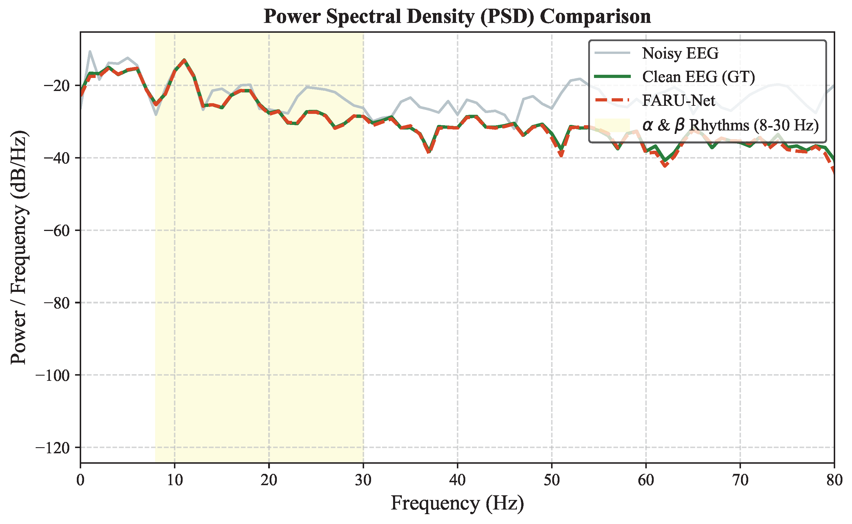
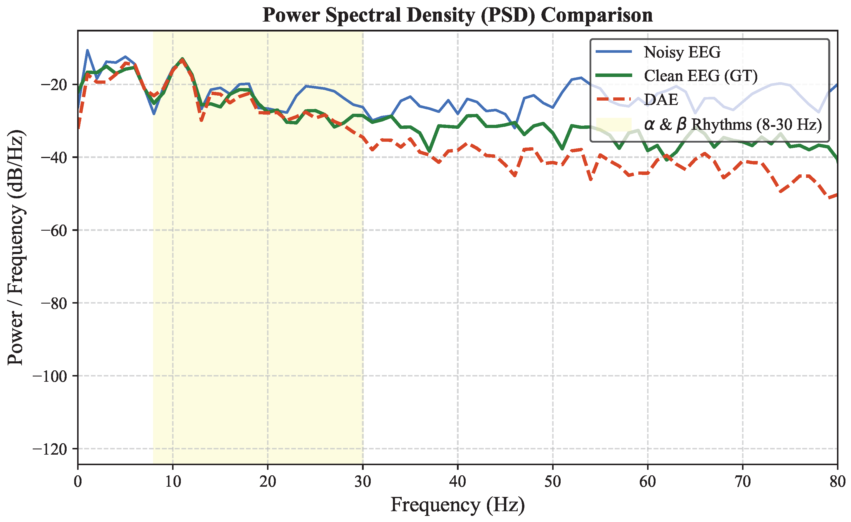
We also evaluate the spectral fidelity of the reconstructed signals through Power Spectral Density (PSD) analysis, as shown in Figure 5. Deep learning models optimized only for the time domain often face the issue of “spectral blurring,” where high-frequency neural signals are unintentionally suppressed along with the artifacts. However, FARU-Net, utilizing the Frequency-aware Bottleneck Module (FBM), maintains excellent spectral consistency. In the yellow-shaded region corresponding to the α and β rhythms (8–30 Hz), FARU-Net closely matches the power distribution of the clean ground truth. At higher frequencies (>30 Hz), FARU-Net effectively attenuates the abnormal energy spikes caused by EMG artifacts, reducing them to the physiological noise floor. Conversely, the PSD curve of the DAE baseline (Figure 6) reveals significant spectral leakage and incomplete artifact suppression in the high-frequency band, further corroborating its suboptimal generalization in mixed-noise scenarios. This qualitative comparison across both time and frequency domains highlights the architectural superiority of FARU-Net in disentangling neural oscillations from complex physiological interference.
While Figure 3, Figure 4, Figure 5 and Figure 6 provide qualitative evidence of FARU-Net’s denoising capability, we further quantify its statistical robustness through 20-fold cross-validation across varying signal-to-noise ratios (Table 8). The fine-grained partitioning ( k = 20 ) provides a more conservative estimate of generalization performance by minimizing the variance introduced by data splitting.

4.7. Cross-Dataset Robustness Evaluation

To evaluate the generalization performance of FARU-Net under unsupervised, real-world conditions, we conducted a zero-shot validation using the C3 channel recordings from the first 30 subjects (S001–S030) of the PhysioNet Motor Imagery (MI) dataset [42]. Unlike the controlled synthetic mixtures used in training, this dataset presents diverse physiological profiles and unmodeled instrumental noise. Given the intrinsic unavailability of ground-truth clean EEG in such scenarios, the Power Reduction Ratio (PRR) is employed as a quantitative proxy for denoising effectiveness, defined as:
PRR = 1 t = 1 T x ^ 2 ( t ) t = 1 T y 2 ( t ) × 100 %
where y ( t ) represents the original contaminated EEG, x ^ ( t ) is the denoised signal generated by FARU-Net, and T is the total length of the recording. Table 9 presents the PRR results across these 30 subjects. It should be noted that while PRR serves as a quantitative proxy for denoising effectiveness in real-world data where ground-truth is unavailable, it is not an absolute denoising metric. A high PRR value does not inherently guarantee signal fidelity, as indiscriminate attenuation of neural components could also yield high values. Therefore, the validity of PRR results must be interpreted alongside the model’s adaptive behavior across diverse noise intensities.
The selection of the first 30 subjects (S001–S030) for zero-shot validation is based on two primary considerations:
  • Coverage of Physiological Diversity:As observed from Table 9, the PRR exhibits significant individual variability, ranging from a minimal noise level (e.g., S025 at 0.91%) to extreme high-intensity artifact interference (e.g., S005 at 48.32%). This broad spectrum indicates that the sample size provides sufficient inter-subject variability to validate the adaptive suppression capability of FARU-Net across diverse physiological profiles.
  • Balance Between Computational Efficiency and Evaluation Depth: Since FARU-Net is designed for high-precision, point-to-point reconstruction, this refined processing workflow incurs substantial computational overhead when applied to the full dataset. Selecting these 30 representative subjects facilitates a comprehensive performance assessment within a resource-constrained environment while maintaining a rigorous depth of evaluation.
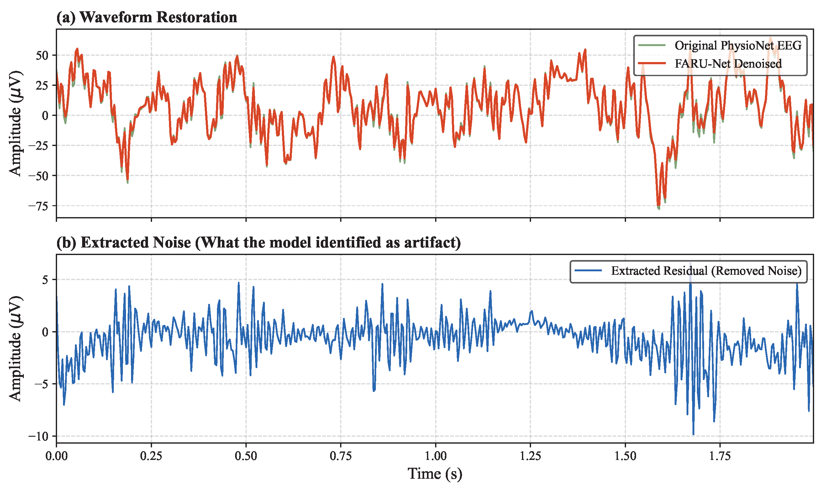
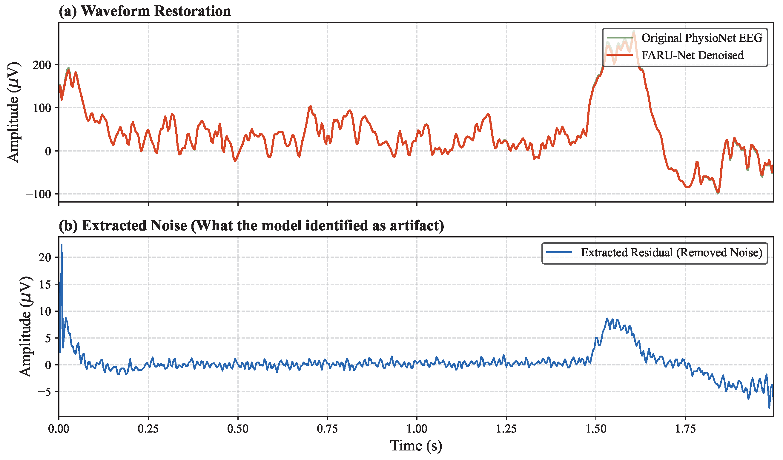
To gain qualitative insight into the model’s adaptability, a comparative residual analysis was conducted under varying recording conditions. As illustrated in Figure 7 and Figure 8, FARU-Net dynamically adjusts its suppression intensity based on the input noise morphology and signal dynamics. Crucially, as detailed in Section 4.8, the subsequent improvement in Motor Imagery classification accuracy (from 79.69% to 81.23%) provides empirical evidence that the power reduction primarily eliminates non-neural interference. If the observed PRR were a result of excessive neural signal attenuation, the downstream decoding performance would inevitably degrade.
In segments characterized by continuous, fine-grained myogenic interference (Figure 7), the residual remains focused on micro-scale stochastic spikes, effectively refining the neural waveform without excessive attenuation of low-amplitude oscillations. Conversely, in scenarios involving extreme signal fluctuations and large-scale baseline drifts (Figure 8), FARU-Net scales its suppression strength to isolate high-amplitude artifacts reaching up to 20 μV. This adaptive, scale-aware mechanism ensures that the model maintains the integrity of rhythmic neural activity even when the signal-to-noise ratio is severely compromised by non-stationary physiological interference [17].
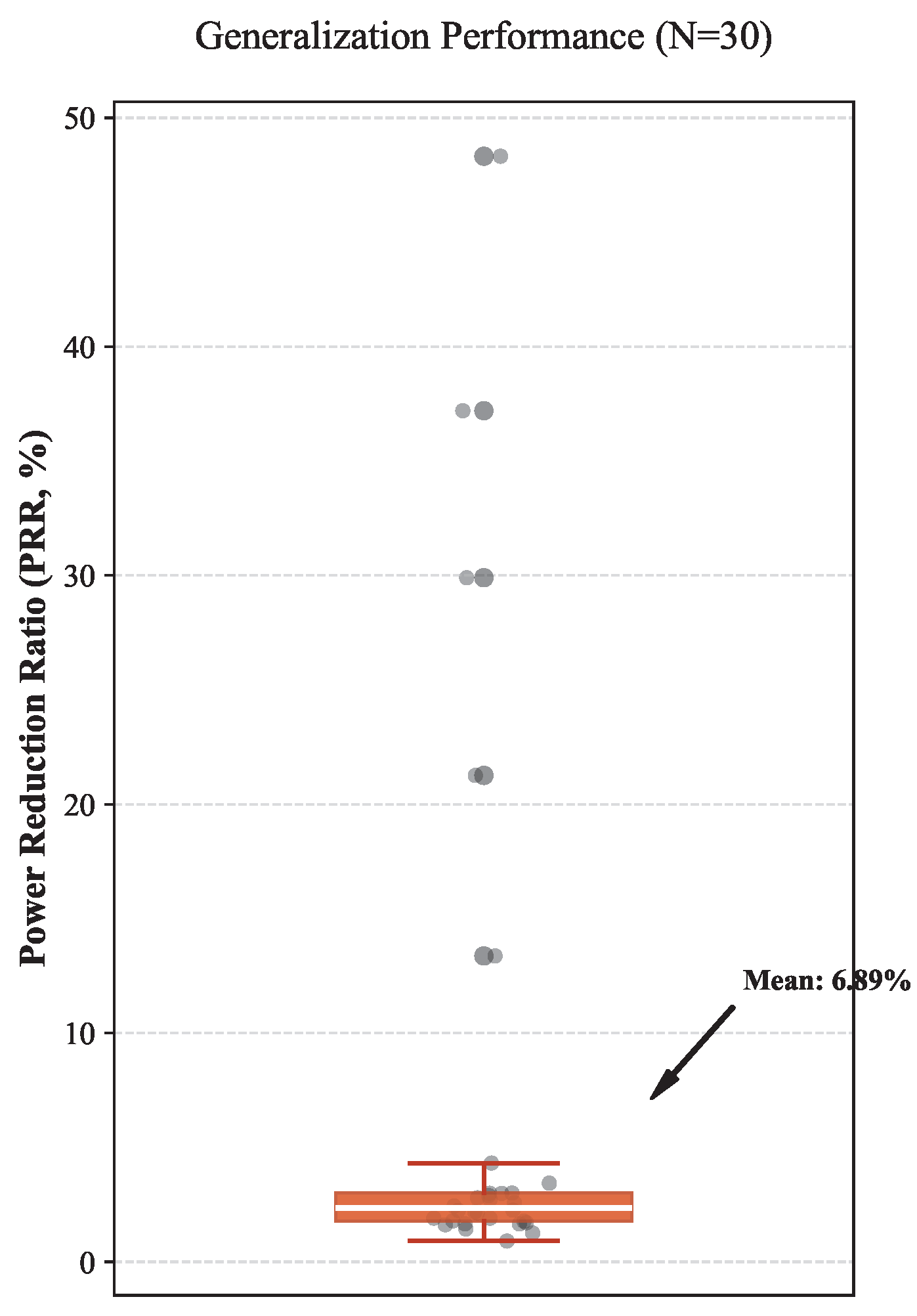
The statistical distribution of PRR values, summarized in Figure 9, further confirms this adaptability. The clear long-tail pattern, with a narrow interquartile range (Median ≈ 2.4%), indicates that the architecture remains conservative for low-noise recordings. Meanwhile, the prominent outliers (up to 48.32%) highlight the model’s capacity to adjust dynamically to suppress high-intensity artifacts when required.

4.8. Downstream BCI Task Validation and Spectral Analysis

While standard metrics like CC and RMSE measure morphological similarity, the practical value of EEG denoising is ultimately reflected in the performance of subsequent analytical tasks. We utilized EEG recordings from the first 30 subjects (S001–S030) of the PhysioNet Motor Movement/Imagery dataset [42,43], specifically the left-hand and right-hand motor imagery trials (runs 4, 8 and 12), to evaluate FARU-Net’s effectiveness in downstream binary classification. To focus the evaluation exclusively on signal quality, we employed a standard, lightweight convolutional classifier (EEGNet [44]) to categorize left- versus right-hand motor execution across three distinct data conditions: raw contaminated EEG, EEG denoised via traditional ICA [21], and EEG denoised by our proposed FARU-Net. The band-specific absolute power of three denoised EEG signals and the classification accuracy of EEGNet model under three kinds of EEG signals are adopted as core evaluation metrics.
To mathematically substantiate the classification results, we conducted a quantitative spectral analysis. The average Absolute Band Power (ABP) was computed using Welch’s method across three key physiological bands: the low-frequency band (1–8 Hz), the motor-imagery specific μ and β band (8–30 Hz), and the high-frequency myogenic band (30–40 Hz). As demonstrated in our spectral analysis (Table 10), FARU-Net achieves a superior balance between artifact suppression and neural signal preservation. While ICA aggressively attenuates low-frequency components, it inadvertently causes a substantial power deficit in the crucial 8–30 Hz neural band (dropping to 267.86 compared to 282.75 for FARU-Net). In contrast, FARU-Net effectively suppresses high-frequency myogenic artifacts (reducing 30–40 Hz power to 48.13) while maintaining robust spectral energy in the task-relevant neural region.
This spectral fidelity is complemented by exceptional preservation of temporal signal integrity (Table 11). Unlike ICA, which severely distorts the signal distribution by reducing kurtosis to 0.4712 (a 60.6% drop from raw) and skewness to 0.2894, FARU-Net maintains the intrinsic non-Gaussian characteristics of neural activity (kurtosis: 1.1169; skewness: 0.5065), closely matching the raw signal statistics. Furthermore, FARU-Net achieves a high correlation with raw EEG ( R = 0.9382 ) and a minimal RMSE ( 2.09 × 10 6 ), confirming that our method removes interference without introducing the waveform distortion or over-smoothing typical of blind source separation techniques.
Collectively, these dual-domain advantages directly translate to enhanced downstream utility. The classifier trained on FARU-Net denoised signals achieved the highest accuracy of 81.23%, outperforming both the raw contaminated data (79.69%) and the ICA baseline (78.93%). This empirical evidence confirms that FARU-Net’s adaptive recalibration effectively reduces non-neural interference while preserving valid EEG signals.

5. Discussion

5.1. Analysis of Performance Margins

The substantial performance advantage of FARU-Net over the baseline models (Table 2) can be attributed to its architectural ability to overcome the inherent limitations of purely temporal or local feature extraction methods. Recent advancements in EEG denoising architectures highlight two critical factors that differentiate superior reconstruction fidelity: (1) the capacity for global temporal modeling and (2) explicit frequency-domain modeling. FARU-Net effectively integrates these capabilities through its Dual-Domain Recalibrationstrategy.
  • Global Dependency Modeling: Conventional baselines such as DAE1D and Simple CNNs typically rely on local convolutional kernels or limited temporal receptive fields. As discussed in recent literature [40], such local operations often struggle to capture long-range dependencies across the EEG sequence. This limitation frequently leads to “spectral blurring”, where the model fails to distinguish between transient neural spikes and broadband artifacts. FARU-Net addresses this by incorporating global temporal modeling mechanisms, which capture context and preserve the temporal continuity of physiological signals far more effectively than standard CNNs.
  • Spectral Fidelity via Frequency-Aware Processing: Models optimized solely in the time domain frequently suffer from spectral distortion, where artifact suppression comes at the cost of attenuating legitimate neural oscillations. Drawing on the insights from time-frequency joint modeling [16], FARU-Net utilizes the Frequency-aware Bottleneck Module (FBM) to perform explicit spectral recalibration. This allows the network to learn distinct representations for artifact components versus neural content in the frequency domain. By isolating and suppressing artifact-dominant frequencies (e.g., high-frequency EMG noise) while protecting the spectral integrity of α and β rhythms, FARU-Net achieves the significant improvements in RRMSE f r e q and SNR observed in the experimental results.
In summary, the significant margin of improvement is not merely a result of deeper networks, but rather the fundamental shift from local, time-domain-only smoothing to a global, dual-domain recalibration process that respects the spectral physiology of EEG signals.

5.2. Phase vs. Magnitude: Robustness in Non-Stationary Signals

The lack of performance gain from explicit phase constraints (Table 5) can be attributed to the intrinsic non-stationarity of EEG signals and the architectural characteristics of FARU-Net. The symmetric skip-connection framework functions as a temporal anchor, facilitating the direct transfer of high-resolution morphological features to the decoder, which maintains sample-level alignment during reconstruction. Furthermore, the FBM utilizes real-valued spectral weights to implement a zero-phase response. This allows for artifact suppression in the latent space without introducing the group delay or temporal shifts characteristic of conventional time-domain filters. Consequently, the dual-domain synergy prioritizes normalized magnitude consistency, which serves as a more stable indicator of underlying brain activity than the volatile phase information. Rapid fluctuations in neural synchrony and phase-locking variability make phase recovery especially difficult in the presence of high-amplitude, stochastic artifacts.
On the other hand, the spectral magnitude constraint focuses on the power distribution of neural rhythms, which serves as a more stable and reliable indicator of underlying brain activity. By prioritizing normalized magnitude consistency, FARU-Net stabilizes the reconstruction process, resulting in the significant ΔSNR improvement observed in the final configuration.

5.3. Physiological Interpretability: The 40 Hz Gamma Focus

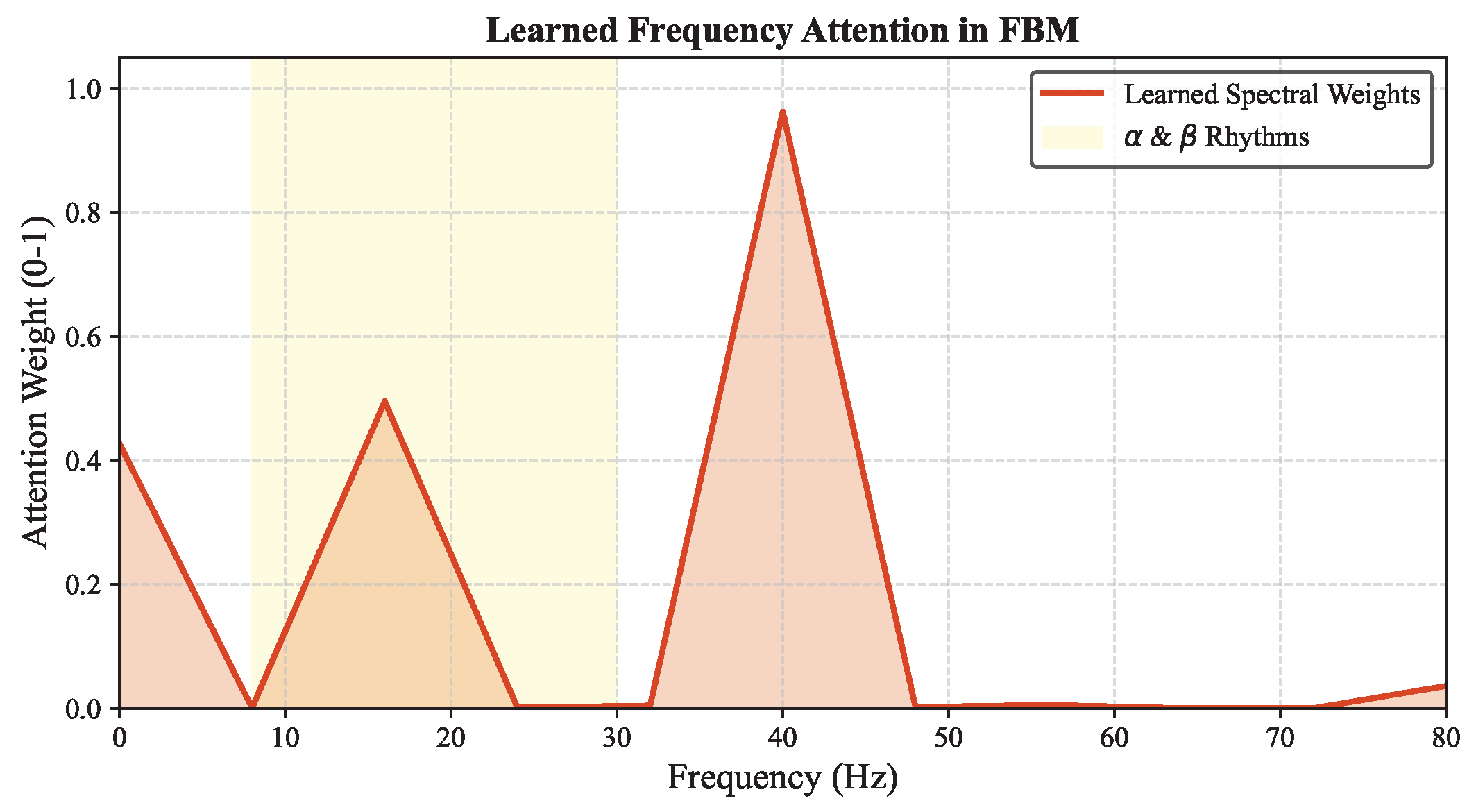
Interpretability analysis of the learned spectral weights w identifies a prominent peak at 40 Hz (Figure 10). This prioritization is a deterministic outcome of data-driven optimization on the EEGdenoiseNet benchmark. Physiologically, the FBM adapts to the frequency-domain SNR profile inherent in the training data: as EOG and EMG spectral power predominantly occupy the sub-8 Hz and supra-50 Hz bands, the 40 Hz region represents a high-fidelity spectral window. The model assigns its highest weights to this band to maximize spectral consistency, reflecting a data-driven convergence to the rhythmic properties of the EEG segments rather than a heuristic assumption.

5.4. Temporal Attention Distribution: Context-Aware Modulation of Skip Features

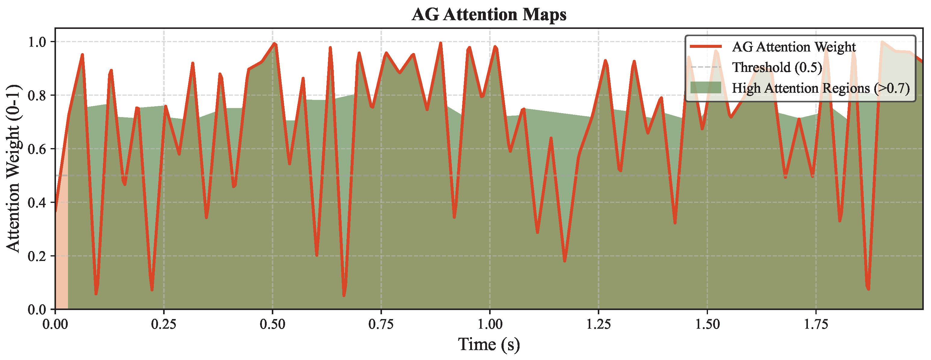
While the FBM governs global spectral consistency, the Attention Gates (AGs) embedded in the skip connections orchestrate local temporal fidelity through a highly dynamic, signal-dependent gating mechanism. Interpretability analysis of the learned temporal attention coefficients α reveals a non-uniform distribution across the time axis (Figure 11), where weights exhibit rapid fluctuations that closely track the instantaneous morphological integrity of the input waveform. Specifically, elevated attention regions ( α > 0.7 , green-shaded zones) consistently align with segments preserving neural oscillations and sharp physiological transients, whereas pronounced troughs ( α < 0.3 , pink-shaded zones) correspond temporally to high-amplitude artifact bursts such as saccadic EOG spikes or broadband myogenic contractions. By dynamically attenuating skip-connection flow during these contaminated intervals, the AG module prevents the decoder from inheriting unrefined noise, effectively bridging the semantic gap between shallow encoder details and deep decoder representations. This data-driven, context-aware “soft thresholding” strategy marks a clear architectural departure from standard U-Net variants, where skip connections often act as passive conduits for residual interference. Ultimately, this localized temporal suppression operates synergistically with the FBM’s global spectral recalibration, collectively enabling high-fidelity signal restoration that preserves both morphological salience and temporal resolution.

5.5. Adaptive Denoising Behavior in Dynamic Environments

A primary challenge in ambulatory EEG monitoring is the non-stationary nature of physiological artifacts. Fixed-threshold filters often struggle in such dynamic environments, leading to either insufficient noise removal or the loss of actual neural data. The cross-dataset validation results and the Power Reduction Ratio (PRR) distribution shown in Figure 6 indicate that FARU-Net exhibits adaptive attenuation behavior. For low-noise segments, the model maintains a low PRR (Median ≈ 2.4%), acting similarly to an identity mapping to preserve signal morphology. During high-amplitude contamination, such as burst EMG, the suppression level increases correspondingly, as shown by the long-tail outliers reaching up to 48.32%. This threshold-free scaling allows the model to respond to varying interference levels. Such adaptability is necessary for practical Brain-Computer Interfaces (BCIs), enabling selective noise reduction while maintaining neural synchrony.

5.6. Computational Efficiency for Wearable Devices

Moreover, FARU-Net achieves this adaptive capability with high computational efficiency through its strategic architectural design. As illustrated in Figure 1, the encoder utilizes four successive downsampling stages via max-pooling, which reduces the temporal dimension of the latent features from the original length L to L = L / 2 4 = L / 16 . Consequently, the Frequency-aware Bottleneck Module (FBM) operates on these highly compressed features. The core computational cost of FBM is dominated by the Real-valued Discrete Fourier Transform (R-DFT). Given that the complexity of a standard Fast Fourier Transform (FFT) for a sequence of length N is O ( N log N ) , the R-DFT complexity in our bottleneck is strictly constrained to O ( L 16 log L 16 ) . For a typical EEG segment where L = 512 , the processing length is reduced to only 32 samples, making the spectral recalibration overhead negligible. In contrast, the initial 1D convolutional layers at the input stage possess a significantly higher complexity of O ( L · C 2 ) , where C is the number of channels.
This scale-aware design facilitates real-time signal restoration without increasing parameter overhead, as quantitatively summarized in Table 12. Although FARU-Net exhibits higher computational complexity than lightweight baselines due to its dual-domain architecture, it maintains an inference speed of 331.65 FPS, well above the 30 FPS threshold required for real-time EEG processing. This favorable trade-off between reconstruction fidelity and computational cost demonstrates that strategically positioning the frequency-aware module at the compressed bottleneck effectively balances performance and efficiency, thereby validating the model’s feasibility for deployment on resource-constrained wearable devices.

6. Conclusions and Future Work

This paper introduced FARU-Net, a dual-domain frequency-aware residual framework designed for high-fidelity EEG artifact removal. By modeling both temporal patterns and spectral hierarchies, the proposed approach addresses the receptive field constraints inherent in traditional time-domain-based deep learning models. The key findings of this study are summarized as follows:
  • Architectural Effectiveness: FARU-Net achieves competitive and effective performance, outperforming baseline models with a mean CC of 0.9681 and a ΔSNR of 26.66 dB.
  • Spectral Recalibration: The Frequency-aware Bottleneck Module (FBM) was instrumental in recalibrating the latent spectrum, enabling adaptive prioritization of crucial neural rhythms.
  • Improved Feature Fusion: The integration of Attention Gates (AGs) successfully reduced the semantic gap between encoder and decoder features, ensuring targeted suppression of residual noise.
  • Dual-Domain Consistency: The joint loss function maintained high consistency between time-domain waveforms and frequency-domain power distributions.
Despite these achievements, several challenges remain. The current model is optimized for single-channel denoising, failing to exploit the strong spatial correlations among multi-channel EEG signals. Restricted by the adopted dataset, this work only targets artifact removal of EOG and EMG interference, without considering other types of noise. Future research will extend the frequency-aware module to multi-channel networks via spatial-temporal-frequency attention mechanisms. We will also explore denoising methods for diverse noise types and improve computational efficiency, facilitating real-time application in wearable EEG monitoring and portable brain-computer interfaces.


Author Contributions

Conceptualization, J.Z. and T.L.; methodology, J.Z.; software, J.Z. and T.C.; validation, J.Z.; formal analysis, J.Z.; investigation, J.Z.; resources, T.L.; data curation, J.Z. and T.C.; writing—original draft preparation, J.Z.; writing—review and editing, T.L., F.L. and Y.J.; visualization, J.Z.; supervision, T.L., F.L. and Y.J. All authors have read and agreed to the published version of the manuscript.

Funding

This research received no external funding.

Data Availability Statement

The data presented in this study are available in the EEGdenoiseNet repository.

Acknowledgments

We thank the contributors of the EEGdenoiseNet dataset.

Conflicts of Interest

The authors declare no conflicts of interest.

References

  1. Mannan, M.M.N.; Kamran, M.A.; Jeong, M.Y. Identification and removal of physiological artifacts from electroencephalogram signals: A review. IEEE Access 2018, 6, 30630–30652. [Google Scholar] [CrossRef]
  2. Jiang, X.; Bian, G.B.; Tian, Z. Removal of artifacts from EEG signals: A review. Sensors 2019, 19, 987. [Google Scholar] [CrossRef] [PubMed]
  3. Raj, V.A.; Parupudi, T.; Thalengala, A.; Nayak, S.G. A comprehensive review of deep learning models for denoising EEG signals: Challenges, advances, and future directions. Discov. Appl. Sci. 2025, 7, 1268. [Google Scholar] [CrossRef]
  4. Thwe, Y.; Maneetham, D.; Crisnapati, P.N. Integrating EEG Artifact Removal with Deep Learning for Accurate Motor Imagery Classification in Acute Stroke. Eng. Technol. Appl. Sci. Res. 2026, 16, 31880–31886. [Google Scholar] [CrossRef]
  5. Zhou, Z.; Rahman Siddiquee, M.M.; Tajbakhsh, N.; Liang, J. Unet++: A nested u-net architecture for medical image segmentation. In Proceedings of the International Workshop on Deep Learning in Medical Image Analysis; Springer: Cham, Switzerland, 2018; pp. 3–11. [Google Scholar]
  6. Azhar, M.; Shafique, T.; Amjad, A. A convolutional neural network for the removal of simultaneous ocular and myogenic artifacts from EEG signals. Electronics 2024, 13, 4576. [Google Scholar] [CrossRef]
  7. Ronneberger, O.; Fischer, P.; Brox, T. U-net: Convolutional networks for biomedical image segmentation. In Proceedings of the International Conference on Medical Image Computing and Computer-Assisted Intervention; Springer: Cham, Switzerland, 2015; pp. 234–241. [Google Scholar]
  8. Chuang, C.H.; Chang, K.Y.; Huang, C.S.; Jung, T.P. IC-U-Net: A U-Net-based denoising autoencoder using mixtures of independent components for automatic EEG artifact removal. NeuroImage 2022, 263, 119586. [Google Scholar] [CrossRef]
  9. Cui, H.; Li, C.; Liu, A.; Qian, R.; Chen, X. A dual-branch interactive fusion network to remove artifacts from single-channel EEG. IEEE Trans. Instrum. Meas. 2023, 73, 4001912. [Google Scholar] [CrossRef]
  10. Chen, J.; Pi, D.; Jiang, X.; Xu, Y.; Chen, Y.; Wang, X. Denosieformer: A transformer-based approach for single-channel EEG artifact removal. IEEE Trans. Instrum. Meas. 2023, 73, 2501116. [Google Scholar] [CrossRef]
  11. Cai, Y.; Meng, Z.; Huang, D. DHCT-GAN: Improving EEG signal quality with a dual-branch hybrid CNN–transformer network. Sensors 2025, 25, 231. [Google Scholar] [CrossRef]
  12. Dewan, D.; Srivastava, A.; Sheet, D. EDGeNet: Electroencephalography Denoising Efficient Network for Fast Artifact Removal. In Proceedings of the 2025 47th Annual International Conference of the IEEE Engineering in Medicine and Biology Society (EMBC); IEEE: Piscataway, NJ, USA, 2025; pp. 1–7. [Google Scholar]
  13. Yin, J.; Liu, A.; Li, C.; Qian, R.; Chen, X. Frequency information enhanced deep EEG denoising network for ocular artifact removal. IEEE Sens. J. 2022, 22, 21855–21865. [Google Scholar] [CrossRef]
  14. Zhang, H.; Zhao, M.; Wei, C.; Mantini, D.; Li, Z.; Liu, Q. EEGdenoiseNet: A benchmark dataset for deep learning solutions of EEG denoising. J. Neural Eng. 2021, 18, 056057. [Google Scholar] [CrossRef]
  15. Wang, H.; Zhang, X.; Xia, Y.; Wu, X. A differential privacy-preserving deep learning caching framework for heterogeneous communication network systems. Int. J. Intell. Syst. 2022, 37, 11142–11166. [Google Scholar] [CrossRef]
  16. Meng, Y.; Yuan, C.; Feng, W.; Li, D.; Nan, J.; Xia, Y.; Zhu, F.; Song, J. TF-Denoiser: A Time-Frequency Domain Joint Method for EEG Artifact Removal. Electronics 2025, 15, 132. [Google Scholar] [CrossRef]
  17. Gabardi, M.; Saibene, A.; Gasparini, F.; Rizzo, D.; Stella, F.A. A multi-artifact EEG denoising by frequency-based deep learning. arXiv 2023, arXiv:2310.17335. [Google Scholar]
  18. Wu, X.; Wang, H.; Zhang, Y.; Li, R. A secure visual framework for multi-index protection evaluation in networks. Digit. Commun. Netw. 2023, 9, 327–336. [Google Scholar] [CrossRef]
  19. Chen, L. Beyond external constraints: The missing dimension of AI governance. SSRN Prepr. 2026. [Google Scholar] [CrossRef]
  20. Chen, J.; Shao, Z.; Zhu, H.; Chen, Y.; Li, Y.; Zeng, Z.; Yang, Y.; Wu, J.; Hu, B. Sustainable interior design: A new approach to intelligent design and automated manufacturing based on Grasshopper. Comput. Ind. Eng. 2023, 183, 109509. [Google Scholar] [CrossRef]
  21. Mammone, N.; La Foresta, F.; Morabito, F.C. Automatic artifact rejection from multichannel scalp EEG by wavelet ICA. IEEE Sens. J. 2011, 12, 533–542. [Google Scholar] [CrossRef]
  22. Zhang, H.; Wei, C.; Zhao, M.; Liu, Q.; Wu, H. A novel convolutional neural network model to remove muscle artifacts from EEG. In Proceedings of the ICASSP 2021–2021 IEEE International Conference on Acoustics, Speech and Signal Processing (ICASSP); IEEE: Piscataway, NJ, USA, 2021; pp. 1265–1269. [Google Scholar]
  23. He, K.; Zhang, X.; Ren, S.; Sun, J. Deep residual learning for image recognition. In Proceedings of the IEEE Conference on Computer Vision and Pattern Recognition, Las Vegas, NV, USA, 27–30 June 2016; pp. 770–778. [Google Scholar]
  24. Rakhmatulin, I.; Dao, M.S.; Nassibi, A.; Mandic, D. Exploring convolutional neural network architectures for EEG feature extraction. Sensors 2024, 24, 877. [Google Scholar] [CrossRef]
  25. Liu, B.; Liu, F.; Song, F. Coupling sPCA-Based Statistical Modeling with Deep Residual Networks Considering Thermal Effect for Deformation Forecasting in High Dams. Struct. Control Health Monit. 2025, 2025, 6688960. [Google Scholar] [CrossRef]
  26. Zhang, Z.; Liu, Q.; Wang, Y. Road Extraction From High-Resolution Remote Sensing Imagery Using Deep Residual U-Net. IEEE Geosci. Remote Sens. Lett. 2018, 15, 749–753. [Google Scholar] [CrossRef]
  27. Achar, D.P.; Bilakeri, S.; Kotegar, K.A.; Radhakrishnan, K. CleanEEG: A U-Net Based Deep Learning Framework for Robust EEG Artifact Removal. Neurosci. Inform. 2026, 6, 100264. [Google Scholar] [CrossRef]
  28. Chang, K.Y.; Huang, Y.C.; Chuang, C.H. Enhancing EEG artifact removal efficiency by introducing dense skip connections to IC-U-Net. In Proceedings of the 2023 45th Annual International Conference of the IEEE Engineering in Medicine & Biology Society (EMBC); IEEE: Piscataway, NJ, USA, 2023; pp. 1–4. [Google Scholar]
  29. Vaswani, A.; Shazeer, N.; Parmar, N.; Uszkoreit, J.; Jones, L.; Gomez, A.N.; Kaiser, Ł.; Polosukhin, I. Attention is all you need. In Advances in Neural Information Processing Systems; NIPS: Red Hook, NY, USA, 2017; Volume 30. [Google Scholar]
  30. Oktay, O.; Schlemper, J.; Folgoc, L.L.; Lee, M.; Heinrich, M.; Misawa, K.; Mori, K.; McDonagh, S.; Hammerla, N.Y.; Kainz, B.; et al. Attention u-net: Learning where to look for the pancreas. arXiv 2018, arXiv:1804.03999. [Google Scholar] [CrossRef]
  31. Lv, H.; Li, C.; Dai, J.; Zhang, Y.; Fan, Z.; Tan, Y.; Wang, D.; Xie, B. Lightweight Framework for Underground Pipeline Recognition and Spatial Localization Based on Multiview 2-D GPR Images. IEEE Trans. Geosci. Remote Sens. 2025, 63, 5110115. [Google Scholar] [CrossRef]
  32. Kołodziej, M.; Jurczak, M.; Majkowski, A.; Rysz, A.; Świderski, B. A hybrid CNN-LSTM approach for muscle artifact removal from EEG using additional EMG signal recording. Appl. Sci. 2025, 15, 4953. [Google Scholar] [CrossRef]
  33. Xiong, W.; Ma, L.; Li, H. A general dual-pathway network for EEG denoising. Front. Neurosci. 2024, 17, 1258024. [Google Scholar] [CrossRef] [PubMed]
  34. Thottempudi, P.; Kumar, V.; Deevi, N. EEG artifact removal strategies for BCI applications: A survey. Majlesi J. Electr. Eng. 2024, 18, 57–72. [Google Scholar]
  35. Jiang, X.; Sun, X.; Hao, Y.; Cai, Q.; Hou, H.; Xia, L.; Li, H.; Li, G.; Gao, Z. WNOTNet: A hybrid wavelet neural operator and transformer framework for enhanced EEG denoising. IEEE Trans. Instrum. Meas. 2025, 74, 1–15. [Google Scholar] [CrossRef]
  36. Asadi-Aghbolaghi, M.; Azad, R.; Fathy, M.; Escalera, S. Multi-level context gating of embedded collective knowledge for medical image segmentation. arXiv 2020, arXiv:2003.05056. [Google Scholar] [CrossRef]
  37. Hossain, M.S.; Mahmud, S.; Khandakar, A.; Al-Emadi, N.; Chowdhury, F.A.; Mahbub, Z.B.; Reaz, M.B.I.; Chowdhury, M.E. MultiResUNet3+: A full-scale connected multi-residual UNet model to denoise electrooculogram and electromyogram artifacts from corrupted electroencephalogram signals. Bioengineering 2023, 10, 579. [Google Scholar] [CrossRef]
  38. Chaurasia, A.; Culurciello, E. Linknet: Exploiting encoder representations for efficient semantic segmentation. In Proceedings of the 2017 IEEE Visual Communications and Image Processing (VCIP); IEEE: Piscataway, NJ, USA, 2017; pp. 1–4. [Google Scholar]
  39. Lin, T.Y.; Dollár, P.; Girshick, R.; He, K.; Hariharan, B.; Belongie, S. Feature pyramid networks for object detection. In Proceedings of the IEEE Conference on Computer Vision and Pattern Recognition, Honolulu, HI, USA, 21–26 July 2017; pp. 2117–2125. [Google Scholar]
  40. Wang, B.; Deng, F.; Jiang, P. EEGDiR: Electroencephalogram denoising network for temporal information storage and global modeling through Retentive Network. Comput. Biol. Med. 2024, 177, 108626. [Google Scholar] [CrossRef] [PubMed]
  41. Wang, D.; Lv, H.; Zhang, Y.; Fan, Z.; Ni, Y.; Lv, S.; Shen, P.; Tang, F.; Wu, H. Monitoring and Detection Technologies and AI-Powered Development Toward Transparent Roads. Engineering 2025, in press. [Google Scholar] [CrossRef]
  42. Schalk, G.; McFarland, D.J.; Hinterberger, T.; Birbaumer, N.; Wolpaw, J.R. BCI2000: A general-purpose brain-computer interface (BCI) system. IEEE Trans. Biomed. Eng. 2004, 51, 1034–1043. [Google Scholar] [CrossRef]
  43. Goldberger, A.L.; Amaral, L.A.; Glass, L.; Hausdorff, J.M.; Ivanov, P.C.; Mark, R.G.; Mietus, J.E.; Moody, G.B.; Peng, C.K.; Stanley, H.E. PhysioBank, PhysioToolkit, and PhysioNet: Components of a new research resource for complex physiologic signals. Circulation 2000, 101, e215–e220. [Google Scholar] [CrossRef]
  44. Lawhern, V.J.; Solon, A.J.; Waytowich, N.R.; Gordon, S.M.; Hung, C.P.; Lance, B.J. EEGNet: A compact convolutional neural network for EEG-based brain–computer interfaces. J. Neural Eng. 2018, 15, 056013. [Google Scholar] [CrossRef] [PubMed]
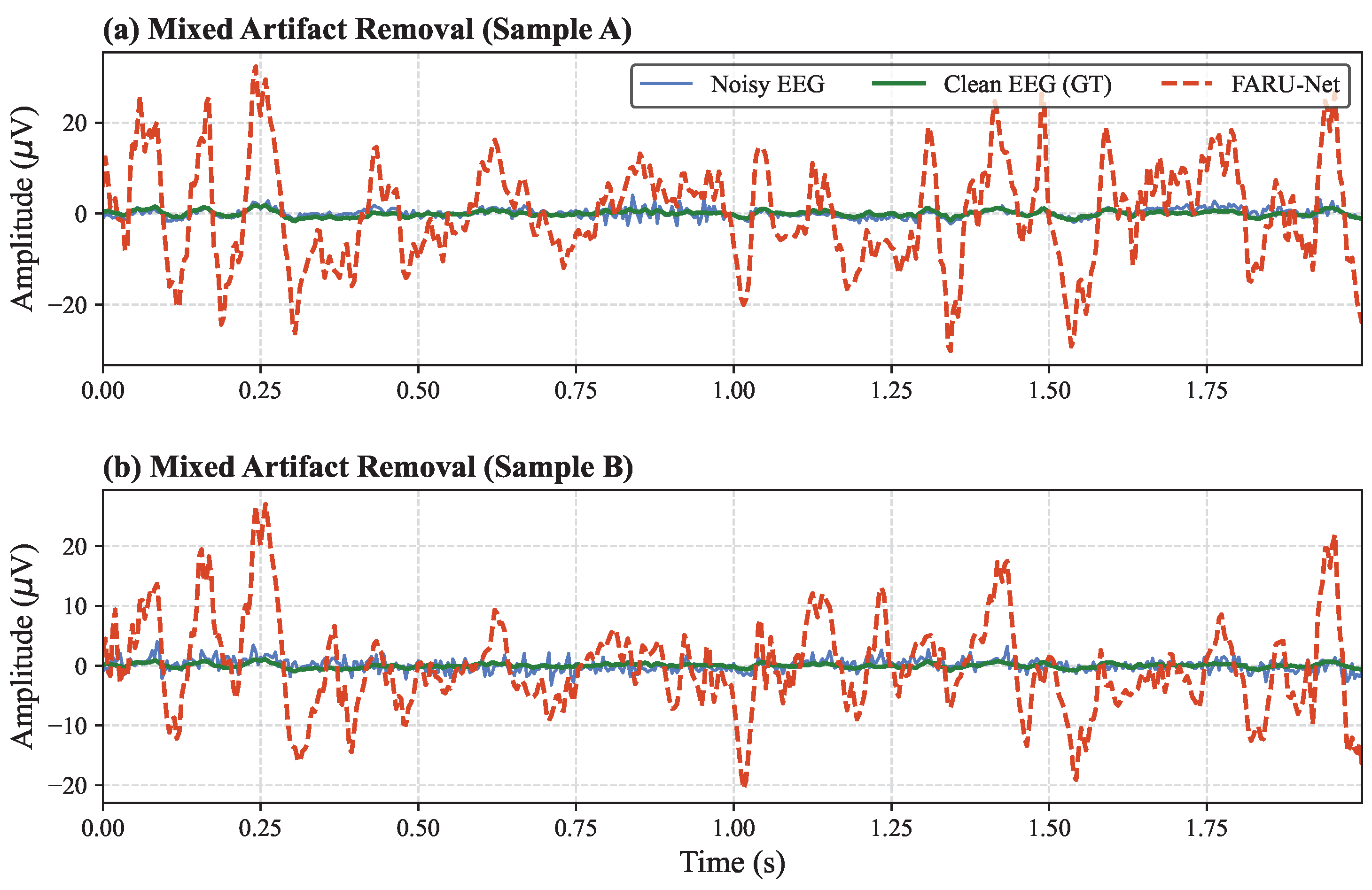
Figure 1. Schematic of the proposed FARU-Net architecture for EEG signal denoising.
Symmetry 18 00988 g001
Figure 2. Time-domain waveforms of the frequency-only model for two representative samples.
Symmetry 18 00988 g002
Figure 3. FARU-Net time-domain denoising results: (a) EOG-contaminated segment; (b) EMG-contaminated segment. The proposed method effectively suppresses artifacts while preserving neural morphology.
Symmetry 18 00988 g003
Figure 4. DAE baseline time-domain denoising results: (a) EOG–contaminated segment; (b) EMG-contaminated segment. Note the residual artifacts compared to FARU–Net.
Symmetry 18 00988 g004
Figure 5. FARU–Net frequency-domain PSD analysis. The yellow region highlights α and β rhythms (8–30 Hz) where FARU–Net demonstrates superior spectral preservation.
Symmetry 18 00988 g005
Figure 6. DAE baseline frequency-domain PSD analysis. Compared to FARU–Net (Figure 5), DAE exhibits greater spectral distortion in the neural band.
Symmetry 18 00988 g006
Figure 7. Adaptive behavior in a segment with fine-grained myogenic interference (standard signal range: ±50 μV).
Symmetry 18 00988 g007
Figure 8. Adaptive behavior in an extreme noise segment featuring large-scale baseline drifts (extreme signal range: + 200 to −100 μV).
Symmetry 18 00988 g008
Figure 9. Statistical distribution of the Power Reduction Ratio (PRR) across 30 subjects. The boxplot reveals a highly adaptive denoising behavior.
Symmetry 18 00988 g009
Figure 10. Spectral interpretive analysis of the FBM. The visualization represents the global frequency attention weights w derived from the EEGdenoiseNet benchmark. The learned profile reveals a strategic prioritization of task-relevant neural oscillations, specifically highlighting the 40 Hz Gamma rhythm and the α / β bands (8–30 Hz). Simultaneously, the module demonstrates an adaptive suppression mechanism targeting non-neural interference, including low-frequency baseline drifts (<8 Hz) and high-frequency broadband myogenic artifacts (>50 Hz).
Symmetry 18 00988 g010
Figure 11. Temporal interpretive analysis of the Attention Gates (AGs). The learned attention coefficients α exhibit dynamic fluctuations across time steps, with high-attention regions ( α > 0.7 ) strategically aligned to salient neural morphology and low-attention troughs ( α < 0.3 ) corresponding to artifact-contaminated segments. This visualization confirms the AG’s role in context-aware feature refinement within skip connections.
Symmetry 18 00988 g011
Table 1. Hardware configurations and hyperparameter settings.
CategoryParameters/Specifications
Hardware
GPUNVIDIA RTX 4090 (24 GB)
CPUIntel Xeon Gold 6430
RAM120 GB
Software
OSUbuntu 22.04
EnvironmentPython 3.12, PyTorch 2.8.0, CUDA 12.8
Training Settings (FARU-Net)
OptimizerAdam
Initial Learning Rate 2.43 × 10 4
Batch Size128
LR SchedulerCosine Annealing (150 epochs)
Training Settings (Baseline Models)
DAE1DAdam, LR: 7.22 × 10 4 , Batch: 32
Complex CNNAdam, LR: 8.25 × 10 4 , Batch: 64
Simple CNNAdam, LR: 9.09 × 10 4 , Batch: 32
FARU-Net Specific
Base Channels/Depth128/4
Optimal λ f 2.16 × 10 4 (Optuna Optimized)
Input Length (L)512 samples (2 s at 256 Hz)
R-DFT Configurationtorch.fft.rfft(real-valued)
Frequency Dimension (F)257 bins ( L / 2 + 1 )
Frequency Resolution0.5 Hz ( f s / L )
Table 2. Performance Comparison of the Proposed FARU-Net and Baseline Models across Various SNR Levels.
MethodMetricSNR (dB)
7 6 5 4 3 2 1 012
FARU-Net R R M S E t i m e 0.47530.38400.31260.25690.21360.18010.15420.13490.12150.1144
R R M S E f r e q 0.36280.28780.23030.18640.15310.12790.10890.09500.08550.0806
C C 0.90960.92640.94020.95190.96190.97030.97720.98260.98650.9891
DAE1D R R M S E t i m e 0.89660.77680.68690.61860.56510.52080.48170.44570.41150.3791
R R M S E f r e q 0.57280.49990.45200.41900.39400.37240.35180.33120.31100.2917
C C 0.65260.70860.75590.79460.82640.85270.87500.89440.91140.9263
Complex CNN R R M S E t i m e 0.90560.77910.68390.61160.55510.50900.46950.43380.40040.3686
R R M S E f r e q 0.57440.49610.44470.40950.38340.36150.34140.32160.30180.2827
C C 0.64960.70830.75820.79930.83250.85930.88140.90010.91620.9302
Simple CNN R R M S E t i m e 1.12860.96360.83830.74210.66610.60300.54820.49840.45280.4116
R R M S E f r e q 0.69330.58960.52550.48590.45830.43490.41140.38680.36150.3372
C C 0.49310.56450.63340.69670.75250.79980.83900.87110.89710.9176
MultiRes-UNet3+ [37] R R M S E t i m e 0.78300.74460.68830.54040.56750.51080.44800.38210.33750.2867
R R M S E f r e q 0.70170.65870.58790.44010.47680.41880.35770.29340.25420.2142
C C 0.61520.65820.71880.81910.82450.85800.89340.92280.94110.9579
LinkNet [38] R R M S E t i m e 0.79890.76380.70880.65320.59940.5370.48210.41430.36100.3107
R R M S E f r e q 0.74470.73990.65780.59690.55590.49720.42620.35760.30480.2622
C C 0.59870.65120.70520.75760.8010.84310.87800.90980.93320.9506
U-Net [7] R R M S E t i m e 0.81220.77550.71890.65240.60170.54580.47360.420770.36030.3118
R R M S E f r e q 0.79030.74290.70880.59990.53410.50270.42870.37630.31340.2635
C C 0.58560.63550.70390.75650.80030.84280.88030.90840.93250.9504
FPN [39] R R M S E t i m e 0.81980.77580.72470.67060.61080.54380.48710.43380.36640.3159
R R M S E f r e q 0.82020.78420.72220.68120.61360.52160.47010.39450.32890.2716
C C 0.57710.6370.69320.75070.79820.84230.87570.90250.93080.9496
Table 3. EMG Artifact Removal: Comparison with Recent Methods (2024–2025) on EEGDenoiseNet (average over SNR 7 to 2 dB).
Method (Year) C C R R M S E t i m e R R M S E f r e q
EEGDiR (2024) [40]0.80720.53220.5004
TF-Denoiser (2025) [16]0.82030.51910.5334
FARU-Net0.90060.35600.2400
Table 4. EOG Artifact Removal: Comparison with Recent Methods (2024–2025) on EEGDenoiseNet (average over SNR 7 to 2 dB).
Method (Year) C C R R M S E t i m e R R M S E f r e q
EEGDiR (2024) [40]0.93290.32790.3616
TF-Denoiser (2025) [16]0.94150.30260.3241
FARU-Net (Ours)0.98560.13860.0997
Table 5. Incremental Ablation Study on Architectural Components. Results are averaged over 5 independent test groups.
ConfigurationCC ↑ RRMSE t RRMSE f ΔSNR (dB) ↑
(a) Base (ResU-Net)0.96550.19460.143823.96
(b) (a) + FBM0.96820.17320.129326.00
(c) (b) + AG0.96770.17740.133425.74
(d) FARU-Net0.96810.17060.127526.66
(e) (d) + L phase 0.96790.17580.132725.95
(f) (b) + L mag 0.96800.17200.128826.40
Table 6. Ablation Study on Network Depth (Number of Downsampling Operations).
DepthCC ↑ RRMSE t RRMSE f ΔSNR (dB) ↑
20.9306 ± 0.00070.3579 ± 0.00190.2529 ± 0.001515.31 ± 0.07
30.9603 ± 0.00060.2287 ± 0.00230.1665 ± 0.002021.44 ± 0.08
4 (Ours)0.9681 ± 0.00070.1706 ± 0.00260.1275 ± 0.002226.66 ± 0.08
Table 7. Ablation Study on Loss Function Components. Results are averaged over 5 independent test groups.
Loss ConfigurationCC ↑ RRMSE t RRMSE f ΔSNR (dB) ↑
Time-only ( L time )0.96770.17740.133425.74
Frequency-only ( L freq )0.860420.402120.3037 20.99
Joint (Ours)0.96810.17060.127526.66
Table 8. Twenty-fold cross-validation performance across varying SNR levels (mean ± std).
SNR (dB)CC ↑ RRMSE t RRMSE f ΔSNR (dB) ↑
7.0 0.9387 ± 0.01220.3231 ± 0.04860.2577 ± 0.041021.34 ± 0.38
6.0 0.9461 ± 0.01090.2666 ± 0.03860.2075 ± 0.031523.12 ± 0.31
5.0 0.9548 ± 0.00910.2189 ± 0.03010.1668 ± 0.024324.67 ± 0.27
4.0 0.9621 ± 0.00780.1824 ± 0.02470.1342 ± 0.019525.89 ± 0.23
3.0 0.9682 ± 0.00650.1609 ± 0.01940.1170 ± 0.014126.71 ± 0.19
2.0 0.9735 ± 0.00510.1421 ± 0.01520.1015 ± 0.010827.28 ± 0.16
1.0 0.9781 ± 0.00390.1268 ± 0.01210.0891 ± 0.008427.69 ± 0.13
0.0 0.9849 ± 0.00280.1085 ± 0.01010.0765 ± 0.006728.15 ± 0.11
1.0 0.9883 ± 0.00190.0992 ± 0.00780.0701 ± 0.005328.42 ± 0.09
2.0 0.9910 ± 0.00150.0928 ± 0.00690.0654 ± 0.004628.61 ± 0.08
Table 9. Quantitative Generalization Performance Across 30 Subjects (PhysioNet MI).
IDPRR (%) σ IDPRR (%) σ
S0011.711.4874S0161.621.8272
S0024.327.3738S01721.269.3757
S0032.251.7807S0183.002.0826
S0042.992.5681S0191.661.8161
S00548.3211.1589S0203.012.4450
S0062.592.0919S0211.441.1330
S00729.908.7613S0222.191.6431
S0081.911.7021S0232.902.5184
S00913.378.1613S02437.208.0927
S0101.661.6771S0250.911.3775
S0112.262.0100S0263.442.5782
S0122.801.9133S0272.142.3390
S0131.782.0392S0282.732.4589
S0141.792.0442S0291.911.6098
S0151.261.4690S0302.442.4199
Overall Average PRR: 6.89%
Table 10. Quantitative comparison of average Absolute Band Power (ABP) across key physiological frequency bands and classification accuracy. Values are scaled by 10 12 for readability. The neural band emphasizes signal preservation, while the EMG band emphasizes artifact suppression.
Data ConditionLow-Freq (1–8 Hz)Neural Band (8–30 Hz)EMG Band (30–40 Hz)Accuracy (%)
Raw Contaminated827.79300.9367.1779.69
ICA Denoised263.81267.8662.9978.93
FARU-Net (Ours)814.55282.7548.1381.23
Table 11. Temporal-domain characteristics comparison across different denoising conditions on PhysioNet Motor Imagery dataset.
MethodKurtosis (↓)|Skewness| (↓)R (vs. Raw)RMSE (vs. Raw)
Raw EEG1.19650.52061.0000 (baseline)0.0000
ICA Denoised0.47120.28940.7827 1.65 × 10 5
FARU-Net (Ours)1.11690.50650.9382 2.09 × 10 6
Table 12. Computational Efficiency Comparison.
ModelFLOPsInference Speed (FPS)
Simple_CNN12.075 M8007.43
DAE1D34.767 M2533.26
Complex_CNN139.919 M3237.20
U-Net1D80.118 M992.43
FARU-Net (Ours)3.302 G331.65
Disclaimer/Publisher’s Note: The statements, opinions and data contained in all publications are solely those of the individual author(s) and contributor(s) and not of MDPI and/or the editor(s). MDPI and/or the editor(s) disclaim responsibility for any injury to people or property resulting from any ideas, methods, instructions or products referred to in the content.