Canal Hypersurfaces Generated by Pseudo-Null Curves with Bishop Frame in Lorentz–Minkowski 4-Space

Abstract

In this paper, we deal with the canal hypersurfaces that are formed as the envelope of a family of pseudo-hyperspheres or pseudo-hyperbolic hyperspheres with centers lying on a pseudo-null curve with Bishop vector fields in four-dimensional Lorentz–Minkowski space. We give main theorems which contain the parametric expressions of these canal hypersurfaces along with their Gaussian, mean, and principal curvatures and important geometric characterizations. We also provide these characterizations for tubular hypersurfaces. Finally, we construct an example to allow for better understanding and comprehension of the results.

1. Introduction

The geometry of hypersurfaces in four-dimensional Lorentz–Minkowski space ${\mathbb{E}}_1^4$, consisting of a semi-Riemannian manifold equipped with an indefinite metric having signature $(-,+,+,+)$, has been a significant subject of study in differential geometry due to its deep connections with mathematical physics, particularly general relativity and the theory of spacetime. Hypersurfaces in ${\mathbb{E}}_1^4$ can be classified as spacelike, timelike, or lightlike according to the causal character of their normal vector fields, leading to a rich variety of geometric and physical behaviors. Exploiting these classifications, several types of (hyper)surfaces (meridian, rotational, canal, dini-type helicoidal, etc.) were examined in [1,2,3,4,5,6]. Among these special hypersurfaces, tubular surfaces are defined as the envelopes of a family of spheres with constant radius having centers that trace a regular space curve. Canal surfaces generalize this concept by allowing the radius to vary smoothly along the curve in [7]. These surfaces play an essential role in understanding the local and global behavior of submanifolds in Euclidean and pseudo-Riemannian settings, particularly due to their well-structured curvature properties and explicit parameterizations. Tubular and canal surfaces naturally arise in various applied contexts where modeling smooth transitions along spatial paths or analyzing flow structures is crucial, including computer-aided geometric design (CAGD), robotics, medical imaging, and fluid dynamics. Their intrinsic and extrinsic geometries provide fertile ground for studying shape operators, geodesics, and curvature invariants, which makes them valuable both from a theoretical perspective and in practical engineering and visualization problems. Taking this into consideration, previous authors have introduced some properties in [8,9,10,11,12,13], while others have addressed applications in [14,15,16,17,18].

As a special class of curves in Lorentzian and more broadly pseudo-Riemannian manifolds, pseudo-null curves have attracted significant interest not only in the realm of differential geometry but also in various applications in theoretical physics. Their intrinsic properties make them valuable tools in the study of spacetime models, particularly within the framework of general relativity, where they can describe degenerate lightlike trajectories or asymptotic causal structures. Moreover, pseudo-null curves emerge in the geometric analysis of wavefronts, gravitational lensing phenomena, and conformal field theories. In mathematical physics, they provide insights into the geometric behavior of solitonic structures and integrable systems. Their role in constructing adapted Frenet frames in Lorentzian geometry further enhances their utility in modeling null-like propagation in relativistic and optical media. Consequently, the study of pseudo-null curves offers not only rich geometric characterizations but also a bridge between abstract mathematical structures and physically meaningful models, as seen in [19,20,21,22,23,24,25].

This paper aims to contribute to the growing body of research by defining canal hypersurfaces generated by pseudo-null curves with Bishop frame in ${\mathbb{E}}_1^4$, with a focus on their differential geometric interpretations in Theorem 1. Additionally, Weingarten maps and Gaussian, mean, and principal curvatures are calculated in Theorem 2. Taking these calculations into consideration, the flatness, minimality, and Weingarten properties of the canal hypersurfaces have been interpreted in Theorem 3. Hence, this study is organized as follows.

In Section 2, some basic definitions and theorems are mentioned about the Bishop frame of a pseudo-null curve and hypersurface theory in Minkowski spacetime. In Section 3, the main theorems of the paper (Theorem 1, Theorem 2, and Theorem 3) are proved in detail. Section 4 contains the geometric properties of tubular hypersurfaces and Section 5 is about the application of the consequences, with some illustrative examples provided to validate the results. Finally, Section 6 summarizes the conclusions and possibilities for further research.

It must be noted that throughout this study we will state $r_s={\displaystyle \frac{dr\left(s\right)}{ds}}$ and $r_{ss}={\displaystyle \frac{d^{2}r\left(s\right)}{d{s}^2}}$. In the sequelae, the factors ${(-1)}^{i!}$ and ${(-\lambda )}^{(5-i)!}$ are used only as compact sign conventions to encode the signs corresponding to the five families and to write them in a unified form.

Theorem 1.

The canal hypersurfaces that are formed as the envelope of a family of pseudo-hyperspheres ($\lambda =1;$$i=1,2,3,4$) or pseudo-hyperbolic hyperspheres ($\lambda =-1;$$i=5$) with centers lying on a pseudo-null curve $\beta \left(s\right)$ with Bishop vector fields $N_j,$ $j\in \{1,2,3,4\}$ in $E_1^4$ can be parametrized by

$$\begin{array}{cc}\hfill & X_i(s,t,w)=\beta \left(s\right)-\lambda r\left(s\right)r_s\left(s\right)N_1\left(s\right)\hfill \\ \hfill & \mp r\left(s\right)\sqrt{{\left(-\lambda \right)}^{(5-i)!}\left(1-\lambda {\left(r_s\left(s\right)\right)}^2\right)}\left(m_{i2}\mathfrak{h}(t,w)N_2\left(s\right)+m_{i3}{N}_3\left(s\right)+{\displaystyle \frac{m_{i4}}{2\mathfrak{h}(t,w)}}{N}_4\left(s\right)\right),\hfill \end{array}$$

(1)

where

$$\left.\begin{array}{c}{m}_{12}=m_{14}=m_{23}=\sin \left(\mathfrak{f}\left(t,w\right)\right),\hfill \\ m_{13}=m_{22}=m_{24}=\cos \left(\mathfrak{f}\left(t,w\right)\right),\hfill \\ m_{32}=m_{43}=m_{53}=-m_{34}=\sinh \left(\mathfrak{f}\left(t,w\right)\right),\hfill \\ m_{33}=m_{42}=m_{52}=-m_{44}=-m_{54}=\cosh \left(\mathfrak{f}\left(t,w\right)\right).\hfill \end{array}\right\}$$

(2)

Here, $r\left(s\right)$ is the radius function, the canal hypersurfaces $X_1(s,t,w),$ $X_2(s,t,w),$ $X_3(s,t,w),$ $X_4(s,t,w)$ are timelike, and the canal hypersurface $X_5(s,t,w)$ is spacelike. We also suppose that ${\left(-\lambda \right)}^{(5-i)!}\left(1-\lambda {\left(r_s\left(s\right)\right)}^2\right)>0;$$\mathfrak{f}\left(t,w\right)$ and $\mathfrak{h}\left(t,w\right)$ are nonzero differentiable functions of t and w, and that the functions $m_{ij}$ are nonzero.

It must be noted here that we give our results (Theorems 2 and 3) and produce their proofs by taking “∓” in (1) as “+”. One can obtain the results by taking “∓” in (1) as “−”. Also, to simplify the notation in the curvature formulas, we introduce the auxiliary functions

$$\Delta \left(s\right)=-\lambda +{\left(r_s\left(s\right)\right)}^2+r\left(s\right)r_{ss}\left(s\right)$$

and

$${\mathsf{\Omega }}_i\left(s\right)=\sqrt{{(-\lambda )}^{(5-i)!}\left(1-\lambda {\left(r_s\left(s\right)\right)}^2\right)}.$$

These notations will be used in the following Gaussian, mean, and principal curvature formulas.

Theorem 2.

The Gaussian curvatures $K_i(s,t,w)$ and mean curvatures $H_i(s,t,w)$ of the canal hypersurfaces $X_i(s,t,w),$ $i\in \{1,2,3,4,5\},$ given by (1) in $E_1^4$ satisfy

$$3H_i(s,t,w)-r^2\left(s\right)K_i(s,t,w)+{\displaystyle \frac{2\lambda {\left(-1\right)}^{i!}}{r\left(s\right)}}=0,$$

(3)

where

$$K_i(s,t,w)={\displaystyle \frac{{\left(-1\right)}^{i!}\left(m_{i2}\mathfrak{h}(t,w){\sigma }_1\left(s\right){\mathsf{\Omega }}_i\left(s\right)-\lambda r_{ss}\left(s\right)\right)}{r^2\left(s\right)\left(\begin{array}{c}\Delta \left(s\right)-\lambda m_{i2}\mathfrak{h}(t,w){\sigma }_1\left(s\right)r\left(s\right){\mathsf{\Omega }}_i\left(s\right)\hfill \end{array}\right)}}$$

(4)

and

$$H_i(s,t,w)={\displaystyle \frac{{\left(-1\right)}^{i!}\left(\begin{array}{c}-3{\left(m_{i2}\right)}^2{\mathfrak{h}}^2(t,w){\left({\sigma }_1\left(s\right)\right)}^2{r}^2\left(s\right){\left({\mathsf{\Omega }}_i\left(s\right)\right)}^2\hfill \\ +{\left(-\lambda \right)}^{(5-i)!}{m}_{i2}\mathfrak{h}(t,w){\sigma }_1\left(s\right)r\left(s\right){\left({\mathsf{\Omega }}_i\left(s\right)\right)}^3\hfill \\ +\Delta \left(s\right)\left(2\Delta \left(s\right)+r\left(s\right)r_{ss}\left(s\right)\right)\hfill \end{array}\right)}{3r\left(s\right)\left(\begin{array}{c}{\left(m_{i2}\right)}^2{\mathfrak{h}}^2(t,w){\left({\sigma }_1\left(s\right)\right)}^2{r}^2\left(s\right)\lambda {\left({\mathsf{\Omega }}_i\left(s\right)\right)}^2-\lambda {\left(\Delta \left(s\right)\right)}^2\hfill \end{array}\right)}}.$$

(5)

Also, the principal curvatures of the canal hypersurfaces $X_i(s,t,w),$ $i\in \{1,2,3,4,5\}$ given by (1) in $E_1^4$ are:

$$\left.\begin{array}{c}{\left(p_1\right)}_i(s,t,w)={\displaystyle \frac{\lambda {(-1)}^{i!}{\sigma }_1\left(s\right){\mathsf{\Omega }}_i\left(s\right)m_{i2}\mathfrak{h}(t,w)-{\left(-1\right)}^{i!}{r}_{ss}\left(s\right)}{\Delta \left(s\right)-\lambda {\sigma }_1\left(s\right)r\left(s\right){\mathsf{\Omega }}_i\left(s\right)m_{i2}\mathfrak{h}(t,w)}},\hfill \\ {\left(p_2\right)}_i(s,t,w)={\left(p_3\right)}_i(s,t,w)={\displaystyle \frac{-{\left(-1\right)}^{i!}}{r\left(s\right)}}.\hfill \end{array}\right\}$$

(6)

Here, ${\sigma }_i\left(s\right)$ are Bishop curvatures of the pseudo null curve and $m_{i2}$ are the coefficient functions given in (2).

Theorem 3.

The canal hypersurfaces $X_i(s,t,w),$ $i\in \{1,2,3,4,5\},$ given by (1) in $E_1^4$ (for $c\in \mathbb{R}$) are

(i) flat if and only if $\mathfrak{h}(t,w)={\displaystyle \frac{c}{m_{i2}}}$ and ${\sigma }_1\left(s\right)={\displaystyle \frac{\lambda r_{ss}\left(s\right)}{c{\mathsf{\Omega }}_i\left(s\right)}}$ hold;

(ii) minimal if and only if $\mathfrak{h}(t,w)={\displaystyle \frac{c}{m_{i2}}}$ and ${\sigma }_1\left(s\right)={\displaystyle \frac{-2+\lambda \left(2{\left(r_s\left(s\right)\right)}^2+3r\left(s\right)r_{ss}\left(s\right)\right)}{3cr\left(s\right){\mathsf{\Omega }}_i\left(s\right)}}$ hold;

(iii) ${\left(H,K\right)}_{st}$-Weingarten and ${\left(H,K\right)}_{sw}$-Weingarten if and only if $\mathfrak{h}(t,w)={\displaystyle \frac{c}{m_{i2}}}$ hold. In addition, they are ${\left(H,K\right)}_{tw}$-Weingarten hypersurfaces.

Here, $m_{i2}$ are the coefficient functions given in (2).

2. Preliminaries

Four-dimensional Lorentz–Minkowski space $E_1^4$ is the real vector space $E^4$ equipped with the standard indefinite flat metric $g(.,.)$ defined for any two vectors $u=(u_1,u_2,u_3,u_4)$ and $v=(v_1,v_2,v_3,v_4)$ in $E_1^4$ by

$$g(u,v)=-u_1{v}_1+u_2{v}_2+u_3{v}_3+u_4{v}_4.$$

A nonzero vector u in $E_1^4$ is spacelike, timelike, or null (lightlike) if $g(u,u)$ is positive, negative, or zero, respectively; in particular, the vector $u=0$ is spacelike. The norm (length) of a vector $u\in E_1^4$ is given by $\parallel u\parallel =\sqrt{\left|g\right(u,u\left)\right|}$. Also, a curve $\beta :I\to E_1^4$ can be locally spacelike, timelike, or null (lightlike) if all of its velocity vectors ${\beta }_s\left(s\right)$ are spacelike, timelike, or null, respectively, where ${\beta }_s\left(s\right)={\displaystyle \frac{d\beta \left(s\right)}{ds}}$ [26].

A pseudo-null curve $\beta :I\to E_1^4$ with Frenet frame $\{T\left(s\right),N\left(s\right),B_1\left(s\right),B_2\left(s\right)\}$ is a spacelike curve for which the principal normal vector $N\left(s\right)$ and second binormal vector $B_2\left(s\right)$ are null vectors. Also, the following conditions are satisfied for a pseudo-null curve:

$$\left.\begin{array}{c}g(T\left(s\right),T\left(s\right))=g(B_1\left(s\right),B_1\left(s\right))=g(N\left(s\right),B_2\left(s\right))=1,\hfill \\ g(N\left(s\right),N\left(s\right))=g(B_2\left(s\right),B_2\left(s\right))=g(T\left(s\right),N\left(s\right))=g(T\left(s\right),B_1\left(s\right))\hfill \\ =g(N\left(s\right),B_1\left(s\right))=g(T\left(s\right),B_2\left(s\right))=g(B_1\left(s\right),B_2\left(s\right))=0.\hfill \end{array}\right\}$$

(7)

The Frenet equations of a pseudo-null curve $\beta \left(s\right)$ in $E_1^4$ are

$$\left.\begin{array}{c}{T}_s\left(s\right)={\kappa }_1\left(s\right)N\left(s\right),N_s\left(s\right)={\kappa }_2\left(s\right)B_1\left(s\right),\hfill \\ {\left(B_1\right)}_s\left(s\right)={\kappa }_3\left(s\right)N\left(s\right)-{\kappa }_2\left(s\right)B_2\left(s\right),{\left(B_2\right)}_s\left(s\right)=-{\kappa }_1\left(s\right)T\left(s\right)-{\kappa }_3\left(s\right)B_1\left(s\right),\hfill \end{array}\right\}$$

(8)

where ${\kappa }_1\left(s\right),$ ${\kappa }_2\left(s\right)$, and ${\kappa }_3\left(s\right)$ are the first, second, and third Frenet curvatures of $\beta \left(s\right)$, respectively, and ${\kappa }_1\left(s\right)=0$ when $\beta \left(s\right)$ is a straight line or ${\kappa }_1\left(s\right)=1$ in all other cases [27,28]. Here, we state $T_s\left(s\right)={\displaystyle \frac{dT\left(s\right)}{ds}}$ and so on. The Frenet frame $\{T\left(s\right),N\left(s\right),B_1\left(s\right),B_2\left(s\right)\}$ is positively oriented if

$$g(T\left(s\right),N\left(s\right)\times B_1\left(s\right)\times B_2\left(s\right))=\det (T\left(s\right),N\left(s\right),B_1\left(s\right),B_2\left(s\right))=1.$$

Note that if $\beta \left(s\right)$ has Frenet curvatures ${\kappa }_2\left(s\right)\ne 0$ and ${\kappa }_3\left(s\right)=0$, then it also lies in $E_1^4$ according to its Frenet Equation (Equation (8)).

In [27], the authors introduced the Bishop frame of a pseudo-null curve $\beta \left(s\right)$ in $E_1^4$ with Frenet curvatures ${\kappa }_1\left(s\right)=1,$ ${\kappa }_2\left(s\right)\ne 0,$ and ${\kappa }_3\left(s\right)=0$ or ${\kappa }_3\left(s\right)\ne 0$. For this purpose, there is a new frame $\{N_1\left(s\right),N_2\left(s\right),N_3\left(s\right),N_4\left(s\right)\}$ along $\beta \left(s\right)$, where $N_2\left(s\right)=N\left(s\right)$ is the principal normal vector field, $N_1\left(s\right)$ and $N_3\left(s\right)$ are spacelike vector fields, and $N_4\left(s\right)$ is a lightlike transversal vector field satisfying

$$\left.\begin{array}{c}g(N_1\left(s\right),N_1\left(s\right))=g(N_3\left(s\right),N_3\left(s\right))=g(N_2\left(s\right),N_4\left(s\right))=1,\hfill \\ g(N_2\left(s\right),N_2\left(s\right))=g(N_4\left(s\right),N_4\left(s\right))=g(N_1\left(s\right),N_2\left(s\right))=g(N_1\left(s\right),N_3\left(s\right))\hfill \\ =g(N_1\left(s\right),N_4\left(s\right))=g(N_2\left(s\right),N_3\left(s\right))=g(N_3\left(s\right),N_4\left(s\right))=0.\hfill \end{array}\right\}$$

(9)

They called the Bishop frame $\{N_1\left(s\right),N_2\left(s\right),N_3\left(s\right),N_4\left(s\right)\}$ of a pseudo-null curve $\beta \left(s\right)$ in $E_1^4$ a positively-oriented pseudo-orthonormal frame containing principal normal vector field $N_2\left(s\right)=N\left(s\right)$, relatively parallel spacelike vector fields $N_1\left(s\right)$ and $N_3\left(s\right)$, and relatively parallel lightlike transversal vector field $N_4\left(s\right)$ satisfying the conditions in (9).

The Bishop frame $\{N_1\left(s\right),N_2\left(s\right),N_3\left(s\right),N_4\left(s\right)\}$ is positively oriented if

$$g(N_1\left(s\right),N_2\left(s\right)\times N_3\left(s\right)\times N_4\left(s\right))=\det (N_1\left(s\right),N_2\left(s\right),N_3\left(s\right),N_4\left(s\right))=1.$$

In [27], the authors proved the following theorem which contains the formulas for pseudo-null curves with Bishop frame.

Theorem 4

([27]). Let $\beta \left(s\right)$ be a pseudo-null curve in $E_1^4$ parameterized by arc length s with Frenet curvatures ${\kappa }_1\left(s\right)=1,$ ${\kappa }_2\left(s\right)\ne 0$, and ${\kappa }_3\left(s\right)$. Then, the Bishop frame $\{N_1\left(s\right),N_2\left(s\right),N_3\left(s\right),N_4\left(s\right)\}$ and Frenet frame $\{T\left(s\right),N\left(s\right),B_1\left(s\right),B_2\left(s\right)\}$ of $\beta \left(s\right)$ are related by

$$\left.\begin{array}{c}{N}_1\left(s\right)={\displaystyle \frac{{\sigma }_2\left(s\right)}{\sqrt{{\left({\sigma }_1\left(s\right)\right)}^2+{\left({\sigma }_2\left(s\right)\right)}^2}}}T\left(s\right)+\left({\displaystyle \frac{{\left({\sigma }_1\left(s\right)\right)}^2{\sigma }_2\left(s\right){\left(\frac{{\sigma }_2\left(s\right)}{{\sigma }_1\left(s\right)}\right)}_s}{{\left({\left({\sigma }_1\left(s\right)\right)}^2+{\left({\sigma }_2\left(s\right)\right)}^2\right)}^2}}-{\displaystyle \frac{{\sigma }_1\left(s\right){\sigma }_3\left(s\right)}{{\left({\sigma }_1\left(s\right)\right)}^2+{\left({\sigma }_2\left(s\right)\right)}^2}}\right)N\left(s\right)\hfill \\ +{\displaystyle \frac{{\sigma }_1\left(s\right)}{\sqrt{{\left({\sigma }_1\left(s\right)\right)}^2+{\left({\sigma }_2\left(s\right)\right)}^2}}}{B}_1\left(s\right),\hfill \\ \\ N_2\left(s\right)=N\left(s\right),\hfill \\ \\ N_3\left(s\right)=-{\displaystyle \frac{{\sigma }_1\left(s\right)}{\sqrt{{\left({\sigma }_1\left(s\right)\right)}^2+{\left({\sigma }_2\left(s\right)\right)}^2}}}T\left(s\right)-\left({\displaystyle \frac{{\left({\sigma }_1\left(s\right)\right)}^3{\left(\frac{{\sigma }_2\left(s\right)}{{\sigma }_1\left(s\right)}\right)}_s}{{\left({\left({\sigma }_1\left(s\right)\right)}^2+{\left({\sigma }_2\left(s\right)\right)}^2\right)}^2}}+{\displaystyle \frac{{\sigma }_2\left(s\right){\sigma }_3\left(s\right)}{{\left({\sigma }_1\left(s\right)\right)}^2+{\left({\sigma }_2\left(s\right)\right)}^2}}\right)N\left(s\right)\hfill \\ +{\displaystyle \frac{{\sigma }_2\left(s\right)}{\sqrt{{\left({\sigma }_1\left(s\right)\right)}^2+{\left({\sigma }_2\left(s\right)\right)}^2}}}{B}_1\left(s\right),\hfill \\ \\ N_4\left(s\right)=-{\displaystyle \frac{{\left({\sigma }_1\left(s\right)\right)}^2{\left(\frac{{\sigma }_2\left(s\right)}{{\sigma }_1\left(s\right)}\right)}_s}{{\left({\left({\sigma }_1\left(s\right)\right)}^2+{\left({\sigma }_2\left(s\right)\right)}^2\right)}^{3/2}}}T\left(s\right)-{\displaystyle \frac{1}{2}}\left({\displaystyle \frac{{\left({\sigma }_3\left(s\right)\right)}^2}{{\left({\sigma }_1\left(s\right)\right)}^2+{\left({\sigma }_2\left(s\right)\right)}^2}}+{\displaystyle \frac{{\left({\left(\frac{{\sigma }_2\left(s\right)}{{\sigma }_1\left(s\right)}\right)}_s\right)}^2{\left({\sigma }_1\left(s\right)\right)}^4}{{\left({\left({\sigma }_1\left(s\right)\right)}^2+{\left({\sigma }_2\left(s\right)\right)}^2\right)}^3}}\right)N\left(s\right)\hfill \\ +{\displaystyle \frac{{\sigma }_3\left(s\right)}{\sqrt{{\left({\sigma }_1\left(s\right)\right)}^2+{\left({\sigma }_2\left(s\right)\right)}^2}}}{B}_1\left(s\right)+B_2\left(s\right)\hfill \end{array}\right\}$$

(10)

and the equations for the Bishop frame read

$$\left[\begin{array}{c}{\left(N_1\left(s\right)\right)}_s\\ {\left(N_2\left(s\right)\right)}_s\\ {\left(N_3\left(s\right)\right)}_s\\ {\left(N_4\left(s\right)\right)}_s\end{array}\right]=\left[\begin{array}{cccc}0& 0& 0& -{\sigma }_1\left(s\right)\\ {\sigma }_1\left(s\right)& {\sigma }_3\left(s\right)& {\sigma }_2\left(s\right)& 0\\ 0& 0& 0& -{\sigma }_2\left(s\right)\\ 0& 0& 0& -{\sigma }_3\left(s\right)\end{array}\right]\left[\begin{array}{c}{N}_1\left(s\right)\\ N_2\left(s\right)\\ N_3\left(s\right)\\ N_4\left(s\right)\end{array}\right],$$

(11)

where the Bishop curvatures ${\sigma }_1\left(s\right),$ ${\sigma }_2\left(s\right)$, and ${\sigma }_3\left(s\right)$ of $\beta \left(s\right)$ have the form

$$\left.\begin{array}{c}{\sigma }_1\left(s\right)={\kappa }_2\left(s\right)\cos \theta \left(s\right),\hfill \\ {\sigma }_2\left(s\right)={\kappa }_2\left(s\right)\sin \theta \left(s\right),\hfill \\ {\sigma }_3\left(s\right)=-{\displaystyle \frac{{\kappa }_2\left(s\right)}{{\theta }_s\left(s\right)}}\left(1+{\left({\displaystyle \frac{{\theta }_s\left(s\right)}{{\kappa }_2\left(s\right)}}\right)}_s\right)\hfill \end{array}\right\}$$

(12)

and the function $\theta \left(s\right)\ne$ constant satisfies the third-order nonlinear differential equation

$$\begin{array}{c}{\left({\displaystyle \frac{1}{{\theta }_s\left(s\right)}}+{\displaystyle \frac{1}{{\theta }_s\left(s\right)}}{\left({\displaystyle \frac{{\theta }_s\left(s\right)}{{\kappa }_2\left(s\right)}}\right)}_s\right)}_s-{\displaystyle \frac{{\kappa }_2\left(s\right)}{2}}{\left({\displaystyle \frac{1}{{\theta }_s\left(s\right)}}+{\displaystyle \frac{1}{{\theta }_s\left(s\right)}}{\left({\displaystyle \frac{{\theta }_s\left(s\right)}{{\kappa }_2\left(s\right)}}\right)}_s\right)}^2\hfill \\ +{\displaystyle \frac{{\left({\theta }_s\left(s\right)\right)}^2}{2{\kappa }_2\left(s\right)}}+{\kappa }_3\left(s\right)=0.\hfill \end{array}$$

(13)

From this theorem, we will assume throughout this study that ${\kappa }_1\left(s\right)=1$ and ${\kappa }_2\left(s\right)\ne 0.$ Hence, from (12), the Bishop curvatures ${\sigma }_1\left(s\right)$ and ${\sigma }_2\left(s\right)$ cannot be zero.

On the other hand, in recent years geometers have been studying the crucial geometric characterizations for various kinds of (hyper)surfaces in four-dimensional spaces ([2,12,29,30,31,32]).

Now, let X be a hypersurface in $E_1^4$ given by

$$\begin{array}{cc}\hfill X:U\subset E^3& ⟶E_1^4\hfill \\ \hfill (s,t,w)& ⟶X(s,t,w)=(X_1(s,t,w),X_2(s,t,w),X_3(s,t,w),X_4(s,t,w)).\hfill \end{array}$$

(14)

The Gauss map (i.e., the unit normal vector field) and the matrix forms of the first and second fundamental forms are

$$\mathcal{N}={\displaystyle \frac{X_s\times X_t\times X_w}{∥X_s\times X_t\times X_w∥}},\left[g_{ij}\right]=\left[\begin{array}{ccc}{g}_{11}& g_{12}& g_{13}\\ g_{21}& g_{22}& g_{23}\\ g_{31}& g_{32}& g_{33}\end{array}\right],\left[h_{ij}\right]=\left[\begin{array}{ccc}{h}_{11}& h_{12}& h_{13}\\ h_{21}& h_{22}& h_{23}\\ h_{31}& h_{32}& h_{33}\end{array}\right],$$

(15)

respectively. Here, $g_{11}=〈X_s,X_s〉,$ $g_{12}=g_{21}=〈X_s,X_t〉,$ $g_{13}=g_{31}=〈X_s,X_w〉,$ $g_{22}=〈X_t,X_t〉,$ $g_{23}=g_{32}=〈X_t,X_w〉,$ $g_{33}=〈X_w,X_w〉;$$h_{11}=〈x_{ss},\mathcal{N}〉,$ $h_{12}=h_{21}=〈x_{st},\mathcal{N}〉,$ $h_{13}=h_{31}=〈x_{sw},\mathcal{N}〉,$ $h_{22}=〈x_{tt},\mathcal{N}〉,$ $h_{23}=h_{32}=〈x_{tw},\mathcal{N}〉,$ $h_{33}=〈x_{ww},\mathcal{N}〉,$ $X_s={\displaystyle \frac{\partial X(s,t,w)}{\partial s}},$ $X_{st}={\displaystyle \frac{{\partial }^{2}X(s,t,w)}{\partial s\partial t}},$ and so on. Also, the matrix of the shape operator of the hypersurface in (14) is

$$S=\left[a_{ij}\right]={\left[g_{ij}\right]}^{-1}\left[h_{ij}\right],$$

(16)

where ${\left[g_{ij}\right]}^{-1}$ is the inverse matrix of $\left[g_{ij}\right]$. With the aid of (15) and (16), the Gaussian curvature and mean curvature of a hypersurface in $E_1^4$ are given by

$$K=\epsilon {\displaystyle \frac{\det \left[h_{ij}\right]}{\det \left[g_{ij}\right]}}\mathrm{and}3\epsilon H=tr\left(S\right),$$

(17)

respectively, where $\epsilon =〈\mathcal{N},\mathcal{N}〉.$ We say that a hypersurface is flat or minimal if it has zero Gaussian or zero mean curvature, respectively. For more details about hypersurfaces in $E_1^4,$ we refer to [30,33], etc.

3. The Proofs of the Main Theorems

3.1. The Proof of Theorem 1

Let the center curve $\beta :I\subseteq \mathbb{R}\to E_1^4$ be a pseudo-null curve with nonzero curvatures with Bishop vector fields $N_1\left(s\right),$ $N_2\left(s\right),$ $N_3\left(s\right),$ $N_4\left(s\right)$. Here, we obtain the canal hypersurfaces that are formed as the envelope of a family of pseudo-hyperspheres and pseudo-hyperbolic hyperspheres with centers lying on a pseudo-null curve $\beta \left(s\right)$ with Bishop vector fields $N_j,$ $j\in \{1,2,3,4\},$ in $E_1^4$.

First, the parameterization of the envelope of pseudo-hyperspheres defining the canal hypersurfaces $X(s,t,w)$ in $E_1^4$ can be given by

$$X(s,t,w)-\beta \left(s\right)=a(s,t,w)N_1\left(s\right)+b(s,t,w)N_2\left(s\right)+c(s,t,w)N_3\left(s\right)+d(s,t,w)N_4\left(s\right),$$

(18)

where $a(s,t,w),$ $b(s,t,w),$ $c(s,t,w),$ and $d(s,t,w)$ are differentiable functions of $s,t,w$ on the interval I. Furthermore, if $X(s,t,w)$ lies on the pseudo-hyperspheres, then it must satisfy the condition

$$g(X(s,t,w)-\beta \left(s\right),X(s,t,w)-\beta \left(s\right))=r^2\left(s\right),$$

(19)

where $r\left(s\right)$ is the radius function. Thus, by using (9) and (18) in (19), we get

$$a^2(s,t,w)+c^2(s,t,w)+2b(s,t,w)d(s,t,w)=r^2\left(s\right).$$

(20)

If we take the derivatives of the expressions in (18) and (20) with respect to s, then we obtain from (11) that

$$\begin{array}{cc}\hfill X_s(s,t,w)& =(1+a_s(s,t,w)+b(s,t,w){\sigma }_1\left(s\right))N_1\left(s\right)\hfill \\ \hfill & +(b_s(s,t,w)+b(s,t,w){\sigma }_3\left(s\right))N_2\left(s\right)\hfill \\ \hfill & +(b(s,t,w){\sigma }_2\left(s\right)+c_s(s,t,w))N_3\left(s\right)\hfill \\ \hfill & +(-a(s,t,w){\sigma }_1\left(s\right)-c(s,t,w){\sigma }_2\left(s\right)+d_s(s,t,w)-d(s,t,w){\sigma }_3\left(s\right))N_4\left(s\right)\hfill \end{array}$$

(21)

and

$$\begin{array}{c}a(s,t,w)a_s(s,t,w)+c(s,t,w)c_s(s,t,w)+b_s(s,t,w)d(s,t,w)+b(s,t,w)d_s(s,t,w)\hfill \\ =r\left(s\right)r_s\left(s\right),\hfill \end{array}$$

(22)

respectively. Moreover, since $X(s,t,w)-\beta \left(s\right)$ is a normal vector to the canal hypersurface, we have

$$g(X(s,t,w)-\beta \left(s\right),X_s(s,t,w))=0.$$

(23)

Thus, from (18), (21), and (23), we reach

$$\begin{array}{c}a(s,t,w)(1+a_s(s,t,w)+b(s,t,w){\sigma }_1\left(s\right))\hfill \\ + b(s,t,w)(-a(s,t,w){\sigma }_1\left(s\right)-c(s,t,w){\sigma }_2\left(s\right)+d_s(s,t,w)-d(s,t,w){\sigma }_3\left(s\right))\hfill \\ + c(s,t,w)(b(s,t,w){\sigma }_2\left(s\right)+c_s(s,t,w))\hfill \\ + d(s,t,w)(b_s(s,t,w)+b(s,t,w){\sigma }_3\left(s\right))=0.\hfill \end{array}$$

(24)

If (22) is used in expression (24), we get

$$a(s,t,w)=-r\left(s\right)r_s\left(s\right),$$

(25)

while if (25) is used in expression (20) we obtain

$$c^2(s,t,w)+2b(s,t,w)d(s,t,w)=r^2\left(s\right)\left(1-{\left(r_s\left(s\right)\right)}^2\right).$$

(26)

From (26), we can write the cases shown below.

• Case 1: $\left\{\begin{array}{c}{b}_1(s,t,w)=\mp r\left(s\right)\sqrt{1-{\left(r_s\left(s\right)\right)}^2}\mathfrak{h}\left(t,w\right)\sin \left(\mathfrak{f}\left(t,w\right)\right)\hfill \\ c_1(s,t,w)=\mp r\left(s\right)\sqrt{1-{\left(r_s\left(s\right)\right)}^2}\cos \left(\mathfrak{f}\left(t,w\right)\right)\hfill \\ d_1(s,t,w)=\mp {\displaystyle \frac{r\left(s\right)\sqrt{1-{\left(r_s\left(s\right)\right)}^2}}{2\mathfrak{h}\left(t,w\right)}}\sin \left(\mathfrak{f}\left(t,w\right)\right)\hfill \end{array}\right\}$
• Case 2: $\left\{\begin{array}{c}{b}_2(s,t,w)=\mp r\left(s\right)\sqrt{1-{\left(r_s\left(s\right)\right)}^2}\mathfrak{h}\left(t,w\right)\cos \left(\mathfrak{f}\left(t,w\right)\right)\hfill \\ c_2(s,t,w)=\mp r\left(s\right)\sqrt{1-{\left(r_s\left(s\right)\right)}^2}\sin \left(\mathfrak{f}\left(t,w\right)\right)\hfill \\ d_2(s,t,w)=\mp {\displaystyle \frac{r\left(s\right)\sqrt{1-{\left(r_s\left(s\right)\right)}^2}}{2\mathfrak{h}\left(t,w\right)}}\cos \left(\mathfrak{f}\left(t,w\right)\right)\hfill \end{array}\right\}$
• Case 3: $\left\{\begin{array}{c}{b}_3(s,t,w)=\mp r\left(s\right)\sqrt{1-{\left(r_s\left(s\right)\right)}^2}\mathfrak{h}\left(t,w\right)\sinh \left(\mathfrak{f}\left(t,w\right)\right)\hfill \\ c_3(s,t,w)=\mp r\left(s\right)\sqrt{1-{\left(r_s\left(s\right)\right)}^2}\cosh \left(\mathfrak{f}\left(t,w\right)\right)\hfill \\ d_3(s,t,w)=\pm {\displaystyle \frac{r\left(s\right)\sqrt{1-{\left(r_s\left(s\right)\right)}^2}}{2\mathfrak{h}\left(t,w\right)}}\sinh \left(\mathfrak{f}\left(t,w\right)\right)\hfill \end{array}\right\}$
• Case 4: $\left\{\begin{array}{c}{b}_4(s,t,w)=\mp r\left(s\right)\sqrt{-1+{\left(r_s\left(s\right)\right)}^2}\mathfrak{h}\left(t,w\right)\cosh \left(\mathfrak{f}\left(t,w\right)\right)\hfill \\ c_4(s,t,w)=\mp r\left(s\right)\sqrt{-1+{\left(r_s\left(s\right)\right)}^2}\sinh \left(\mathfrak{f}\left(t,w\right)\right)\hfill \\ d_4(s,t,w)=\pm {\displaystyle \frac{r\left(s\right)\sqrt{-1+{\left(r_s\left(s\right)\right)}^2}}{2\mathfrak{h}\left(t,w\right)}}\cosh \left(\mathfrak{f}\left(t,w\right)\right)\hfill \end{array}\right\}$
• Therefore, the canal hypersurfaces are represented for $i=1,2,3,4$ by

$$\left.\begin{array}{c}{X}_1(s,t,w)=\beta \left(s\right)-r\left(s\right)r_s\left(s\right)N_1\left(s\right)\hfill \\ \mp r\left(s\right)\sqrt{1-{\left(r_s\left(s\right)\right)}^2}\left(\begin{array}{c}\mathfrak{h}\left(t,w\right)\sin \left(\mathfrak{f}\left(t,w\right)\right)N_2\left(s\right)+\cos \left(\mathfrak{f}\left(t,w\right)\right)N_3\left(s\right)\hfill \\ +{\displaystyle \frac{\sin \left(f\left(t,w\right)\right)}{2\mathfrak{h}\left(t,w\right)}}{N}_4\left(s\right)\hfill \end{array}\right),\hfill \\ X_2(s,t,w)=\beta \left(s\right)-r\left(s\right)r_s\left(s\right)N_1\left(s\right)\hfill \\ \mp r\left(s\right)\sqrt{1-{\left(r_s\left(s\right)\right)}^2}\left(\begin{array}{c}\mathfrak{h}\left(t,w\right)\cos \left(\mathfrak{f}\left(t,w\right)\right)N_2\left(s\right)+\sin \left(\mathfrak{f}\left(t,w\right)\right)N_3\left(s\right)\hfill \\ +{\displaystyle \frac{\cos \left(\mathfrak{f}\left(t,w\right)\right)}{2\mathfrak{h}\left(t,w\right)}}{N}_4\left(s\right)\hfill \end{array}\right),\hfill \\ X_3(s,t,w)=\beta \left(s\right)-r\left(s\right)r_s\left(s\right)N_1\left(s\right)\hfill \\ \mp r\left(s\right)\sqrt{1-{\left(r_s\left(s\right)\right)}^2}\left(\begin{array}{c}\mathfrak{h}\left(t,w\right)\sinh \left(\mathfrak{f}\left(t,w\right)\right)N_2\left(s\right)+\cosh \left(\mathfrak{f}\left(t,w\right)\right)N_3\left(s\right)\hfill \\ -{\displaystyle \frac{\sinh \left(\mathfrak{f}\left(t,w\right)\right)}{2\mathfrak{h}\left(t,w\right)}}{N}_4\left(s\right)\hfill \end{array}\right),\hfill \\ X_4(s,t,w)=\beta \left(s\right)-r\left(s\right)r_s\left(s\right)N_1\left(s\right)\hfill \\ \mp r\left(s\right)\sqrt{-1+{\left(r_s\left(s\right)\right)}^2}\left(\begin{array}{c}\mathfrak{h}\left(t,w\right)\cosh \left(\mathfrak{f}\left(t,w\right)\right)N_2\left(s\right)+\sinh \left(\mathfrak{f}\left(t,w\right)\right)N_3\left(s\right)\hfill \\ -{\displaystyle \frac{\cosh \left(\mathfrak{f}\left(t,w\right)\right)}{2\mathfrak{h}\left(t,w\right)}}{N}_4\left(s\right)\hfill \end{array}\right),\hfill \end{array}\right\}$$

(27)

which are the first four cases ($i=1,2,3,4$) of the expression in (1).

Second, if $X(s,t,w)$ lies on the pseudo-hyperbolic hyperspheres, then it must satisfy the condition

$$g(X(s,t,w)-\beta \left(s\right),X(s,t,w)-\beta \left(s\right))=-r^2\left(s\right).$$

(28)

Through a similar method as above, by using (28) we have $a(s,t,w)=r\left(s\right)r_s\left(s\right)$ and

• Case 5: $\left\{\begin{array}{c}{b}_5(s,t,w)=\mp r\left(s\right)\sqrt{1+{\left(r_s\left(s\right)\right)}^2}\mathfrak{h}\left(t,w\right)\cosh \left(\mathfrak{f}\left(t,w\right)\right)\hfill \\ c_5(s,t,w)=\mp r\left(s\right)\sqrt{1+{\left(r_s\left(s\right)\right)}^2}\sinh \left(\mathfrak{f}\left(t,w\right)\right)\hfill \\ d_5(s,t,w)=\pm {\displaystyle \frac{r\left(s\right)\sqrt{1+{\left(r_s\left(s\right)\right)}^2}}{2\mathfrak{h}\left(t,w\right)}}\cosh \left(\mathfrak{f}\left(t,w\right)\right)\hfill \end{array}\right\}$
• and so

$$\begin{array}{cc}\hfill & X_5(s,t,w)=\beta \left(s\right)+r\left(s\right)r_s\left(s\right)N_1\left(s\right)\hfill \\ \hfill & \mp r\left(s\right)\sqrt{1+{\left(r_s\left(s\right)\right)}^2}\left(\begin{array}{c}\mathfrak{h}\left(t,w\right)\cosh \left(\mathfrak{f}\left(t,w\right)\right)N_2\left(s\right)+\sinh \left(\mathfrak{f}\left(t,w\right)\right)N_3\left(s\right)\hfill \\ -{\displaystyle \frac{\cosh \left(\mathfrak{f}\left(t,w\right)\right)}{2\mathfrak{h}\left(t,w\right)}}{N}_4\left(s\right)\hfill \end{array}\right),\hfill \end{array}$$

(29)

which is the fifth case ($i=5$) of the expression in (1). Thus, the proof is complete.

3.2. The Proof of Theorem 2

In this subsection, we will give the proof for the canal hypersurface $X_1(s,t,w)$. The proofs for the other canal hypersurfaces $X_i,$ $(i=2,3,4,5)$ can be done similarly.

Here, it must be noted that from now on we will state $N_i=N_i\left(s\right)$, $\mathfrak{f}=\mathfrak{f}(t,w)$, $\mathfrak{h}=\mathfrak{h}(t,w),$ $\sin \mathfrak{f}=\sin \left(\mathfrak{f}\right(t,w\left)\right),$ ${\mathfrak{f}}_t={\displaystyle \frac{\partial \mathfrak{f}(t,w)}{\partial t}},$ ${\mathfrak{f}}_{tt}={\displaystyle \frac{{\partial }^2\mathfrak{f}(t,w)}{\partial t^2}},$ and so on. Also, all results below are considered on the regular part of the parameterization, where the first fundamental form is non-degenerate. In particular, we assume $\det \left(g_{ij}\right)\ne 0$. We also assume that all denominator terms appearing in the curvature formulas are nonzero.

First, from (11), the first derivatives according to $s,$ $t,$ and w of the canal hypersurface $X_1(s,t,w)$ are obtained as

$$\left.\begin{array}{c}{\left(X_1\right)}_s=\left(1-r_s^2+{\sigma }_{1}r\sqrt{1-r_s^2}\mathfrak{h}\sin \mathfrak{f}-r{r}_{ss}\right)N_1\hfill \\ +{\displaystyle \frac{\left(\left({\sigma }_{3}r+r_s\right)\left(1-r_s^2\right)-r{r}_s{r}_{ss}\right)\mathfrak{h}\sin \mathfrak{f}}{\sqrt{1-r_s^2}}}{N}_2+{\displaystyle \frac{{\sigma }_{2}r\left(1-r_s^2\right)\mathfrak{h}\sin \mathfrak{f}-r_s\left(-1+r_s^2+r{r}_{ss}\right)\cos \mathfrak{f}}{\sqrt{1-r_s^2}}}{N}_3\hfill \\ +{\displaystyle \frac{2r\mathfrak{h}\left({\sigma }_1{r}_s\sqrt{1-r_s^2}-{\sigma }_2\left(1-r_s^2\right)\cos \mathfrak{f}\right)-\left(\left({\sigma }_{3}r-r_s\right)\left(1-r_s^2\right)+r{r}_s{r}_{ss}\right)\sin \mathfrak{f}}{2\sqrt{1-r_s^2}\mathfrak{h}}}{N}_4,\hfill \\ {\left(X_1\right)}_t=r\sqrt{1-r_s^2}\left({\mathfrak{hf}}_t\cos \mathfrak{f}+{\mathfrak{h}}_t\sin \mathfrak{f}\right)N_2-r\sqrt{1-r_s^2}{\mathfrak{f}}_t\sin \mathfrak{f}{N}_3\hfill \\ +{\displaystyle \frac{r\sqrt{1-r_s^2}\left({\mathfrak{hf}}_t\cos \mathfrak{f}-{\mathfrak{h}}_t\sin \mathfrak{f}\right)}{2{\mathfrak{h}}^2}}{N}_4,\hfill \\ {\left(X_1\right)}_w=r\sqrt{1-r_s^2}\left({\mathfrak{hf}}_w\cos \mathfrak{f}+{\mathfrak{h}}_w\sin \mathfrak{f}\right)N_2-r\sqrt{1-r_s^2}{\mathfrak{f}}_w\sin \mathfrak{f}{N}_3\hfill \\ +{\displaystyle \frac{r\sqrt{1-r_s^2}\left({\mathfrak{hf}}_w\cos \mathfrak{f}-{\mathfrak{h}}_w\sin \mathfrak{f}\right)}{2{\mathfrak{h}}^2}}{N}_4,\hfill \end{array}\right\}$$

(30)

respectively. From (15) and (30), the unit normal vector field ${\mathcal{N}}_1$ of $X_1$ in $E_1^4$ is

$${\mathcal{N}}_1=r_s{N}_1-\sqrt{1-r_s^2}\mathfrak{h}\sin \mathfrak{f}{N}_2-\sqrt{1-r_s^2}\cos \mathfrak{f}{N}_3-{\displaystyle \frac{1}{2\mathfrak{h}}}\sqrt{1-r_s^2}\sin \mathfrak{f}{N}_4,$$

(31)

and so we get

$$ϵ=g({\mathcal{N}}_1,{\mathcal{N}}_1)=1.$$

(32)

Also, the coefficients of the first fundamental form of $X_1$ are

$$\left.\begin{array}{c}{\left(g_{11}\right)}_1={\displaystyle \frac{\left(\begin{array}{c}{r}^2\left({\sigma }_1^2+{\sigma }_2^2\right){\left(-1+r_s^2\right)}^2{\mathfrak{h}}^2{\sin }^2\mathfrak{f}-{\sigma }_3^2{r}^2{\left(-1+r_s^2\right)}^2{\sin }^2\mathfrak{f}\hfill \\ +{\left(-1+r_s^2+r{r}_{ss}\right)}^2\hfill \\ -2r\mathfrak{h}\sin \mathfrak{f}\left(\begin{array}{c}r{\left(-1+r_s^2\right)}^2{\sigma }_2{\sigma }_3\cos \mathfrak{f}\hfill \\ +{\sigma }_1\sqrt{1-r_s^2}\left(\left(1+{\sigma }_{3}r{r}_s\right)\left(-1+r_s^2\right)+r{r}_{ss}\right)\hfill \end{array}\right)\hfill \end{array}\right)}{1-r_s^2}},\hfill \\ {\left(g_{12}\right)}_1={\left(g_{21}\right)}_1={\displaystyle \frac{r^2\left(\begin{array}{c}{\mathfrak{h}}^2\left({\sigma }_1{r}_s\sqrt{1-r_s^2}\cos \mathfrak{f}+{\sigma }_2\left(-1+r_s^2\right)\right){\mathfrak{f}}_t\hfill \\ +{\sigma }_3\left(-1+r_s^2\right){\mathfrak{h}}_t{\sin }^2\mathfrak{f}\hfill \\ +\mathfrak{h}\sin \mathfrak{f}\left({\sigma }_1{r}_s\sqrt{1-r_s^2}+{\sigma }_2\left(-1+r_s^2\right)\cos \mathfrak{f}\right){\mathfrak{h}}_t\hfill \end{array}\right)}{\mathfrak{h}}},\hfill \\ {\left(g_{13}\right)}_1={\left(g_{31}\right)}_1={\displaystyle \frac{r^2\left(\begin{array}{c}{\mathfrak{h}}^2\left({\sigma }_1{r}_s\sqrt{1-r_s^2}\cos \mathfrak{f}+{\sigma }_2\left(-1+r_s^2\right)\right){\mathfrak{f}}_w\hfill \\ +{\sigma }_3\left(-1+r_s^2\right){\mathfrak{h}}_w{\sin }^2\mathfrak{f}\hfill \\ +\mathfrak{h}\sin \mathfrak{f}\left({\sigma }_1{r}_s\sqrt{1-r_s^2}+{\sigma }_2\left(-1+r_s^2\right)\cos \mathfrak{f}\right){\mathfrak{h}}_w\hfill \end{array}\right)}{\mathfrak{h}}},\hfill \\ {\left(g_{22}\right)}_1=-{\displaystyle \frac{r^2\left(-1+r_s^2\right)\left({\mathfrak{f}}_t^2{\mathfrak{h}}^2-{\mathfrak{h}}_t^2{\sin }^2\mathfrak{f}\right)}{{\mathfrak{h}}^2}},\hfill \\ {\left(g_{23}\right)}_1={\left(g_{32}\right)}_1=-{\displaystyle \frac{r^2\left(-1+r_s^2\right)\left({\mathfrak{f}}_t{\mathfrak{f}}_w{\mathfrak{h}}^2-{\mathfrak{h}}_t{\mathfrak{h}}_w{\sin }^2\mathfrak{f}\right)}{{\mathfrak{h}}^2}},\hfill \\ {\left(g_{33}\right)}_1=-{\displaystyle \frac{r^2\left(-1+r_s^2\right)\left({\mathfrak{f}}_w^2{\mathfrak{h}}^2-{\mathfrak{h}}_w^2{\sin }^2\mathfrak{f}\right)}{{\mathfrak{h}}^2}}\hfill \end{array}\right\}$$

(33)

and it follows that

$$\begin{array}{cc}\hfill & \det \left[{\left(g_{ij}\right)}_1\right]\hfill \\ \hfill & ={\displaystyle \frac{r^4}{{\mathfrak{h}}^2}}\left(-1+r_s^2\right){\sin }^2\mathfrak{f}{\left({\sigma }_{1}r\sqrt{1-r_s^2}\mathfrak{h}\sin \mathfrak{f}-\left(-1+r_s^2+r{r}_{ss}\right)\right)}^2{\left({\mathfrak{f}}_t{\mathfrak{h}}_w-{\mathfrak{f}}_w{\mathfrak{h}}_t\right)}^2.\hfill \end{array}$$

(34)

By using (11) in (30) and obtaining the second derivatives ${\left(X_1\right)}_{ss},$ ${\left(X_1\right)}_{st},$ ${\left(X_1\right)}_{sw},$ ${\left(X_1\right)}_{tt},$ ${\left(X_1\right)}_{tw}$, and ${\left(X_1\right)}_{ww}$ of $X_1$, we obtain the coefficients of the second fundamental form of $X_1$ from (31) as follows:

$$\left.\begin{array}{c}{\left(h_{11}\right)}_1={\displaystyle \frac{\left(\begin{array}{c}2\left({\sigma }_1^2+{\sigma }_2^2\right)r{\left(-1+r_s^2\right)}^2{\mathfrak{h}}^2{\sin }^2\mathfrak{f}-2{\sigma }_3^{2}r{\left(-1+r_s^2\right)}^2{\sin }^2\mathfrak{f}\hfill \\ +2r_{ss}\left(-1+r_s^2+r{r}_{ss}\right)\hfill \\ -2\mathfrak{h}\sin \mathfrak{f}\left(\begin{array}{c}2{\sigma }_2{\sigma }_{3}r{\left(-1+r_s^2\right)}^2\cos \mathfrak{f}\hfill \\ +{\sigma }_1\sqrt{1-r_s^2}\left(\left(1+2{\sigma }_{3}r{r}_s\right)\left(-1+r_s^2\right)+2r{r}_{ss}\right)\hfill \end{array}\right)\hfill \end{array}\right)}{2\left(1-r_s^2\right)}},\hfill \\ {\left(h_{12}\right)}_1={\left(h_{21}\right)}_1=r\left(\begin{array}{c}\mathfrak{h}\left({\sigma }_1{r}_s\sqrt{1-r_s^2}\cos \mathfrak{f}+{\sigma }_2\left(-1+r_s^2\right)\right){\mathfrak{f}}_t\hfill \\ +{\displaystyle \frac{1}{\mathfrak{h}}}{\sigma }_3\left(-1+r_s^2\right){\mathfrak{h}}_t{\sin }^2\mathfrak{f}\hfill \\ +\sin \mathfrak{f}\left({\sigma }_1{r}_s\sqrt{1-r_s^2}+{\sigma }_2\left(-1+r_s^2\right)\cos \mathfrak{f}\right){\mathfrak{h}}_t\hfill \end{array}\right),\hfill \\ {\left(h_{13}\right)}_1={\left(h_{31}\right)}_1=r\left(\begin{array}{c}\mathfrak{h}\left({\sigma }_1{r}_s\sqrt{1-r_s^2}\cos \mathfrak{f}+{\sigma }_2\left(-1+r_s^2\right)\right){\mathfrak{f}}_w\hfill \\ +{\displaystyle \frac{1}{\mathfrak{h}}}{\sigma }_3\left(-1+r_s^2\right){\mathfrak{h}}_w{\sin }^2\mathfrak{f}\hfill \\ +\sin \mathfrak{f}\left({\sigma }_1{r}_s\sqrt{1-r_s^2}+{\sigma }_2\left(-1+r_s^2\right)\cos \mathfrak{f}\right){\mathfrak{h}}_w\hfill \end{array}\right),\hfill \\ {\left(h_{22}\right)}_1=-{\displaystyle \frac{1}{{\mathfrak{h}}^2}}r\left(-1+r_s^2\right)\left({\mathfrak{f}}_t^2{\mathfrak{h}}^2-{\mathfrak{h}}_t^2{\sin }^2\mathfrak{f}\right),\hfill \\ {\left(h_{23}\right)}_1={\left(h_{32}\right)}_1=-{\displaystyle \frac{1}{{\mathfrak{h}}^2}}r\left(-1+r_s^2\right)\left({\mathfrak{f}}_t{\mathfrak{f}}_w{\mathfrak{h}}^2-{\mathfrak{h}}_t{\mathfrak{h}}_w{\sin }^2\mathfrak{f}\right),\hfill \\ {\left(h_{33}\right)}_1=-{\displaystyle \frac{1}{{\mathfrak{h}}^2}}r\left(-1+r_s^2\right)\left({\mathfrak{f}}_w^2{\mathfrak{h}}^2-{\mathfrak{h}}_w^2{\sin }^2\mathfrak{f}\right)\hfill \end{array}\right\}$$

(35)

and so

$$\begin{array}{cc}\hfill & \det \left[{\left(h_{ij}\right)}_1\right]\hfill \\ \hfill & =-{\displaystyle \frac{r^2\left(-1+r_s^2\right){\sin }^2\mathfrak{f}{\left({\mathfrak{f}}_t{\mathfrak{h}}_w-{\mathfrak{h}}_t{\mathfrak{f}}_w\right)}^2}{{\mathfrak{h}}^2}}\left(\begin{array}{c}{\sigma }_1^{2}r\left(-1+r_s^2\right){\mathfrak{h}}^2{\sin }^2\mathfrak{f}\hfill \\ -r_{ss}\left(-1+r_s^2+r{r}_{ss}\right)\hfill \\ +{\sigma }_1\sqrt{1-r_s^2}\left(-1+r_s^2+2r{r}_{ss}\right)\mathfrak{h}\sin \mathfrak{f}\hfill \end{array}\right).\hfill \end{array}$$

(36)

Thus, from (17), (34), and (36) we obtain the Gaussian curvature of $X_1$ as

$$K_1={\displaystyle \frac{-{\sigma }_1\sqrt{1-r_s^2}\mathfrak{h}\sin \mathfrak{f}+r_{ss}}{r^2\left(-1+r_s^2-{\sigma }_{1}r\sqrt{1-r_s^2}\mathfrak{h}\sin \mathfrak{f}+r{r}_{ss}\right)}}.$$

(37)

Using (16), (33), and (35), we obtain the components of the shape operator matrix

$$S_1=\left[\begin{array}{ccc}{\left(S_1\right)}_{11}& {\left(S_1\right)}_{12}& {\left(S_1\right)}_{13}\\ {\left(S_1\right)}_{21}& {\left(S_1\right)}_{22}& {\left(S_1\right)}_{23}\\ {\left(S_1\right)}_{31}& {\left(S_1\right)}_{32}& {\left(S_1\right)}_{33}\end{array}\right]$$

(38)

as

$$\left.\begin{array}{c}{\left(S_1\right)}_{11}={\displaystyle \frac{{\sigma }_1^{2}r\left(-1+r_s^2\right){\mathfrak{h}}^2{\sin }^2\mathfrak{f}-r_{ss}\left(-1+r_s^2+r{r}_{ss}\right)+{\sigma }_1\sqrt{1-r_s^2}\mathfrak{h}\sin \mathfrak{f}\left(-1+r_s^2+2r{r}_{ss}\right)}{{\sigma }_1^2{r}^2\left(-1+r_s^2\right){\mathfrak{h}}^2{\sin }^2\mathfrak{f}+2{\sigma }_{1}r\sqrt{1-r_s^2}\left(-1+r_s^2+r{r}_{ss}\right)\mathfrak{h}\sin \mathfrak{f}-{\left(-1+r_s^2+r{r}_{ss}\right)}^2}},\hfill \\ {\left(S_1\right)}_{21}=\hfill \\ {\displaystyle \frac{\begin{array}{c}{\sigma }_{1}r\left(-1+r_s^2\right){\mathfrak{h}}^3\left({\sigma }_1{r}_s-{\sigma }_2\sqrt{1-r_s^2}\cos \mathfrak{f}\right){\mathfrak{f}}_w\hfill \\ +\mathfrak{h}\left(-1+r_s^2+r{r}_{ss}\right)\left({\sigma }_1{r}_s\sqrt{1-r_s^2}{\mathfrak{h}}_w\cos \mathfrak{f}+\left(-1+r_s^2\right)\left({\sigma }_3{\mathfrak{f}}_w+{\sigma }_2{\mathfrak{h}}_w\right)\right)\hfill \\ +{\mathfrak{h}}^2\left(\begin{array}{c}{\sigma }_1\sqrt{1-r_s^2}\csc \mathfrak{f}(-\left(({\sigma }_{3}r{\sin }^2\mathfrak{f}-r_s)\left(-1+r_s^2\right)\right)+r{r}_s{r}_{ss}){\mathfrak{f}}_w\hfill \\ +\cos \mathfrak{f}\sin \mathfrak{f}{\sigma }_1^{2}r{r}_s\left(-1+r_s^2\right){\mathfrak{h}}_w\hfill \\ +{\sigma }_2\left(-1+r_s^2\right)\left(\begin{array}{c}\cot \mathfrak{f}\left(-1+r_s^2+r{r}_{ss}\right){\mathfrak{f}}_w\\ -{\sigma }_{1}r\sqrt{1-r_s^2}{\mathfrak{h}}_w\sin \mathfrak{f}\left)\right)\end{array}\right)\hfill \end{array}\right)\hfill \end{array}}{r\left({\sigma }_1^2{r}^2\left(-1+r_s^2\right){\mathfrak{h}}^2{\sin }^2\mathfrak{f}+2{\sigma }_{1}r\sqrt{1-r_s^2}\left(-1+r_s^2+r{r}_{ss}\right)\mathfrak{h}\sin \mathfrak{f}-{\left(-1+r_s^2+r{r}_{ss}\right)}^2\right)\left({\mathfrak{f}}_t{\mathfrak{h}}_w-{\mathfrak{h}}_t{\mathfrak{f}}_w\right)}},\hfill \\ {\left(S_1\right)}_{31}=\hfill \\ {\displaystyle \frac{\begin{array}{c}-4{\sigma }_{1}r\left(-1+r_s^2\right){\mathfrak{h}}^3\left({\sigma }_1{r}_s-{\sigma }_2\sqrt{1-r_s^2}\cos \mathfrak{f}\right){\mathfrak{f}}_t\hfill \\ -4\mathfrak{h}\left(-1+r_s^2+r{r}_{ss}\right)\left({\sigma }_1{r}_s\sqrt{1-r_s^2}{\mathfrak{h}}_t\cos \mathfrak{f}+\left(-1+r_s^2\right)\left({\sigma }_3{\mathfrak{f}}_t+{\sigma }_2{\mathfrak{h}}_t\right)\right)\hfill \\ +4{\mathfrak{h}}^2\left(\begin{array}{c}-{\sigma }_1\sqrt{1-r_s^2}\csc \mathfrak{f}\left(-\left(({\sigma }_{3}r{\sin }^2\mathfrak{f}-r_s)\left(-1+r_s^2\right)\right)+r{r}_s{r}_{ss}\right){\mathfrak{f}}_t\hfill \\ -\frac{1}{2}{\sigma }_1^{2}r{r}_s\left(-1+r_s^2\right)\sin \left(2\mathfrak{f}\right){\mathfrak{h}}_t\hfill \\ -{\sigma }_2\left(-1+r_s^2\right)\left(\begin{array}{c}\cot \mathfrak{f}\left(-1+r_s^2+r{r}_{ss}\right){\mathfrak{f}}_t\\ -{\sigma }_{1}r\sqrt{1-r_s^2}{\mathfrak{h}}_t\sin \mathfrak{f}\left)\right)\end{array}\right)\hfill \end{array}\right)\hfill \end{array}}{4r\left({\sigma }_1^2{r}^2\left(-1+r_s^2\right){\mathfrak{h}}^2{\sin }^2\mathfrak{f}+2{\sigma }_{1}r\sqrt{1-r_s^2}\left(-1+r_s^2+r{r}_{ss}\right)\mathfrak{h}\sin \mathfrak{f}-{\left(-1+r_s^2+r{r}_{ss}\right)}^2\right)\left({\mathfrak{f}}_t{\mathfrak{h}}_w-{\mathfrak{h}}_t{\mathfrak{f}}_w\right)}},\hfill \\ {\left(S_1\right)}_{12}={\left(S_1\right)}_{13}={\left(S_1\right)}_{23}={\left(S_1\right)}_{32}=0,{\left(S_1\right)}_{22}={\left(S_1\right)}_{33}={\displaystyle \frac{1}{r}}.\hfill \end{array}\right\}$$

(39)

Thus, from (17) and (39) we obtain the mean curvature of $X_1$ as

$$H_1={\displaystyle \frac{\left(\begin{array}{c}3{\sigma }_1^2{r}^2\left(-1+r_s^2\right){\mathfrak{h}}^2{\sin }^2\mathfrak{f}+{\sigma }_{1}r{\left(1-r_s^2\right)}^{3/2}\mathfrak{h}\sin \mathfrak{f}\hfill \\ +\left(-1+r_s^2+r{r}_{ss}\right)\left(-2+2r_s^2+3r{r}_{ss}\right)\hfill \end{array}\right)}{3r\left({\sigma }_1^2{r}^2\left(-1+r_s^2\right){\mathfrak{h}}^2{\sin }^2\mathfrak{f}+{\left(-1+r_s^2+r{r}_{ss}\right)}^2\right)}}.$$

(40)

Therefore, we obtain the relation between the Gaussian and mean curvatures of the canal hypersurface $X_1$ from (37) and (40) as

$$3H_1-r^2\left(s\right)K_1-{\displaystyle \frac{2}{r\left(s\right)}}=0.$$

(41)

Now, we can find the principal curvatures ${\left(p_1\right)}_1$, ${\left(p_2\right)}_1$ and ${\left(p_3\right)}_1$ of $X_1$ with the help of characteristic values under the condition

$$\det (S_1-{\left(p\right)}_1{I}_3)=0.$$

(42)

Using (39) in (42), we get

$${\left(p_1\right)}_1={\displaystyle \frac{-{\sigma }_1\sqrt{1-r_s^2}\mathfrak{h}\sin \mathfrak{f}+r_{ss}}{-1+r_s^2-{\sigma }_{1}r\sqrt{1-r_s^2}\mathfrak{h}\sin \mathfrak{f}+r{r}_{ss}}},{\left(p_2\right)}_1={\left(p_3\right)}_1={\displaystyle \frac{1}{r}}.$$

(43)

Hence (37), (40), (41), and (43) prove Theorem 2 for canal hypersurface $X_1$. Using a similar procedure for the other canal hypersurfaces $X_i,$ $i=2,3,4,5,$ we can obtain their Gaussian curvatures $K_i$, mean curvatures $H_i$, and principal curvatures ${\left(p_1\right)}_i$, ${\left(p_2\right)}_i$, and ${\left(p_3\right)}_i$ as

$$\left.\begin{array}{c}{K}_2={\displaystyle \frac{{\sigma }_1\sqrt{1-r_s^2}\mathfrak{h}\cos \mathfrak{f}-r_{ss}}{r^2\left(-1+r_s^2-{\sigma }_{1}r\sqrt{1-r_s^2}\mathfrak{h}\cos \mathfrak{f}+r{r}_{ss}\right)}}\hfill \\ K_3={\displaystyle \frac{{\sigma }_1\sqrt{1-r_s^2}\mathfrak{h}\sinh \mathfrak{f}-r_{ss}}{r^2\left(-1+r_s^2-{\sigma }_{1}r\sqrt{1-r_s^2}\mathfrak{h}\sinh \mathfrak{f}+r{r}_{ss}\right)}}\hfill \\ K_4={\displaystyle \frac{{\sigma }_1\sqrt{-1+r_s^2}\mathfrak{h}\cosh \mathfrak{f}-r_{ss}}{r^2\left(-1+r_s^2-{\sigma }_{1}r\sqrt{-1+r_s^2}\mathfrak{h}\cosh \mathfrak{f}+r{r}_{ss}\right)}}\hfill \\ K_5={\displaystyle \frac{{\sigma }_1\sqrt{1+r_s^2}\mathfrak{h}\cosh \mathfrak{f}+r_{ss}}{r^2\left(1+r_s^2+{\sigma }_{1}r\sqrt{1+r_s^2}\mathfrak{h}\cosh \mathfrak{f}+r{r}_{ss}\right)}}\hfill \end{array}\right\}$$

(44)

$$\left.\begin{array}{c}{H}_2=-{\displaystyle \frac{3{\sigma }_1^2{r}^2\left(-1+r_s^2\right){\mathfrak{h}}^2{\cos }^2\mathfrak{f}+{\sigma }_{1}r{\left(1-r_s^2\right)}^{3/2}\mathfrak{h}\cos \mathfrak{f}+\left(-1+r_s^2+r{r}_{ss}\right)\left(-2+2r_s^2+3r{r}_{ss}\right)}{3r\left({\sigma }_1^2{r}^2\left(-1+r_s^2\right){\mathfrak{h}}^2{\cos }^2\mathfrak{f}+{\left(-1+r_s^2+r{r}_{ss}\right)}^2\right)}}\hfill \\ H_3=-{\displaystyle \frac{3{\sigma }_1^2{r}^2\left(-1+r_s^2\right){\mathfrak{h}}^2{\sinh }^2\mathfrak{f}+{\sigma }_{1}r{\left(1-r_s^2\right)}^{3/2}\mathfrak{h}\sinh \mathfrak{f}+\left(-1+r_s^2+r{r}_{ss}\right)\left(-2+2r_s^2+3r{r}_{ss}\right)}{3r\left({\sigma }_1^2{r}^2\left(-1+r_s^2\right){\mathfrak{h}}^2{\sinh }^2\mathfrak{f}+{\left(-1+r_s^2+r{r}_{ss}\right)}^2\right)}}\hfill \\ H_4=-{\displaystyle \frac{3{\sigma }_1^2{r}^2\left(1-r_s^2\right){\mathfrak{h}}^2{\cosh }^2\mathfrak{f}-{\sigma }_{1}r{\left(-1+r_s^2\right)}^{3/2}\mathfrak{h}\cosh \mathfrak{f}+\left(-1+r_s^2+r{r}_{ss}\right)\left(-2+2r_s^2+3r{r}_{ss}\right)}{3r\left({\sigma }_1^2{r}^2\left(1-r_s^2\right){\mathfrak{h}}^2{\cosh }^2\mathfrak{f}+{\left(-1+r_s^2+r{r}_{ss}\right)}^2\right)}}\hfill \\ H_5=-{\displaystyle \frac{3{\sigma }_1^2{r}^2\left(-1-r_s^2\right){\mathfrak{h}}^2{\cosh }^2\mathfrak{f}+{\sigma }_{1}r{\left(1+r_s^2\right)}^{3/2}\mathfrak{h}\cosh \mathfrak{f}+\left(1+r_s^2+r{r}_{ss}\right)\left(2+2r_s^2+3r{r}_{ss}\right)}{3r\left({\sigma }_1^2{r}^2\left(1+r_s^2\right){\mathfrak{h}}^2{\cosh }^2\mathfrak{f}-{\left(1+r_s^2+r{r}_{ss}\right)}^2\right)}}\hfill \end{array}\right\}$$

(45)

$$\left.\begin{array}{c}\left\{{\left(p_1\right)}_2={\displaystyle \frac{{\sigma }_1\sqrt{1-r_s^2}\mathfrak{h}\cos \mathfrak{f}-r_{ss}}{-1+r_s^2-{\sigma }_{1}r\sqrt{1-r_s^2}\mathfrak{h}\cos \mathfrak{f}+r{r}_{ss}}},{\left(p_2\right)}_2={\left(p_3\right)}_2=-{\displaystyle \frac{1}{r}}\right\}\hfill \\ \left\{{\left(p_1\right)}_3={\displaystyle \frac{{\sigma }_1\sqrt{1-r_s^2}\mathfrak{h}\sinh \mathfrak{f}-r_{ss}}{-1+r_s^2-{\sigma }_{1}r\sqrt{1-r_s^2}\mathfrak{h}\sinh \mathfrak{f}+r{r}_{ss}}},{\left(p_2\right)}_3={\left(p_3\right)}_3=-{\displaystyle \frac{1}{r}}\right\}\hfill \\ \left\{{\left(p_1\right)}_4={\displaystyle \frac{{\sigma }_1\sqrt{-1+r_s^2}\mathfrak{h}\cosh \mathfrak{f}-r_{ss}}{-1+r_s^2-{\sigma }_{1}r\sqrt{-1+r_s^2}\mathfrak{h}\cosh \mathfrak{f}+r{r}_{ss}}},{\left(p_2\right)}_4={\left(p_3\right)}_4=-{\displaystyle \frac{1}{r}}\right\}\hfill \\ \left\{{\left(p_1\right)}_5={\displaystyle \frac{-{\sigma }_1\sqrt{1+r_s^2}\mathfrak{h}\cosh \mathfrak{f}-r_{ss}}{1+r_s^2+{\sigma }_{1}r\sqrt{1+r_s^2}\mathfrak{h}\cosh \mathfrak{f}+r{r}_{ss}}},{\left(p_2\right)}_5={\left(p_3\right)}_5=-{\displaystyle \frac{1}{r}}\right\}\hfill \end{array}\right\}$$

(46)

and the relations between the Gaussian and mean curvatures as

$$\left.\begin{array}{c}3H_2-r^2{K}_2+{\displaystyle \frac{2}{r}}=0\hfill \\ 3H_3-r^2{K}_3+{\displaystyle \frac{2}{r}}=0\hfill \\ 3H_4-r^2{K}_4+{\displaystyle \frac{2}{r}}=0\hfill \\ 3H_5-r^2{K}_5-{\displaystyle \frac{2}{r}}=0.\hfill \end{array}\right\}$$

(47)

Thus, the proof is complete.

3.3. The Proof of Theorem 3

We will prove this theorem for $X_1$; the proofs for the other canal hypersurfaces can be performed similarly.

(i) From (37), if the canal hypersurface $X_1$ is flat, then we have

$$\mathfrak{h}\sin \mathfrak{f}={\displaystyle \frac{r_{ss}}{{\sigma }_1\sqrt{1-r_s^2}}}.$$

(48)

Since the left side of (48) depends on $\{t,w\}$ and the right side depends on s, both sides of Equation (48) must be constant. Taking

$$\mathfrak{h}\sin \mathfrak{f}={\displaystyle \frac{r_{ss}}{{\sigma }_1\sqrt{1-r_s^2}}}=c,(c\in \mathbb{R}),$$

we get $\mathfrak{h}={\displaystyle \frac{c}{\sin \mathfrak{f}}}$ and ${\sigma }_1={\displaystyle \frac{r_{ss}}{c\sqrt{1-r_s^2}}}$. Conversely, if we take $\mathfrak{h}={\displaystyle \frac{c}{\sin \mathfrak{f}}}$ and ${\sigma }_1={\displaystyle \frac{r_{ss}}{c\sqrt{1-r_s^2}}}$ in (37), we get $K_1=0$, meaning that $X_1$ is flat.

(ii) From (40), if the canal hypersurface $X_1$ is minimal, then we have

$$\begin{array}{c}3{\sigma }_1^2{r}^2\left(-1+r_s^2\right){\mathfrak{h}}^2{\sin }^2\mathfrak{f}+{\sigma }_{1}r{\left(1-r_s^2\right)}^{3/2}\mathfrak{h}\sin \mathfrak{f}\hfill \\ +\left(-1+r_s^2+r{r}_{ss}\right)\left(-2+2r_s^2+3r{r}_{ss}\right)=0.\hfill \end{array}$$

(49)

From (49), it must be the case that $\mathfrak{h}={\displaystyle \frac{c}{\sin f}},$ ($c\in \mathbb{R}$). Using this in (40), we obtain $H_1$ as

$$H_1={\displaystyle \frac{cr\left(3cr{\sigma }_1\left(-1+r_s^2\right)+\sqrt{1-r_s^2}\left(-2+2r_s^2+3r{r}_{ss}\right)\right)}{3c{r}^2\sqrt{1-r_s^2}\left(-1+r_s^2-cr{\sigma }_1\sqrt{1-r_s^2}+r{r}_{ss}\right)}}.$$

(50)

If $X_1$ is minimal, then from (50) we get

$$cr\left(3cr{\sigma }_1\left(-1+r_s^2\right)+\sqrt{1-r_s^2}\left(-2+2r_s^2+3r{r}_{ss}\right)\right)=0,$$

and by solving this equation we have ${\sigma }_1={\displaystyle \frac{-2+2r_s^2+3r{r}_{ss}}{3cr\sqrt{1-r_s^2}}}$. Conversely, if $\mathfrak{h}={\displaystyle \frac{c}{\sin \mathfrak{f}}}$ and ${\sigma }_1={\displaystyle \frac{-2+2r_s^2+3r{r}_{ss}}{3cr\sqrt{1-r_s^2}}}$ ($c\in \mathbb{R}$), then we have $H_1=0$, meaning that $X_1$ is minimal.

(iii) From (37) and (40), we get

$${\left(H_1\right)}_s{\left(K_1\right)}_t-{\left(K_1\right)}_s{\left(H_1\right)}_t=-{\displaystyle \frac{2{\sigma }_1{r}_s{\left(1-r_s^2\right)}^{5/2}\left({\mathfrak{hf}}_t\cos \mathfrak{f}+{\mathfrak{h}}_t\sin \mathfrak{f}\right)}{3r_s^4{\left(1-r_s^2+{\sigma }_{1}r\sqrt{1-r_s^2}\mathfrak{h}\sin \mathfrak{f}-r{r}_{ss}\right)}^3}}.$$

(51)

From (51), the canal hypersurface $X_1$ is ${\left(H,K\right)}_{st}$-Weingarten if and only if

$$2{\sigma }_1{r}_s{\left(1-r_s^2\right)}^{5/2}\left({\mathfrak{hf}}_t\cos \mathfrak{f}+{\mathfrak{h}}_t\sin \mathfrak{f}\right)=0.$$

(52)

By solving (52), we get $\mathfrak{h}=c\csc \mathfrak{f}$ ($c\in \mathbb{R}$).

From (37) and (40), we get

$${\left(H_1\right)}_s{\left(K_1\right)}_w-{\left(K_1\right)}_s{\left(H_1\right)}_w=-{\displaystyle \frac{2{\sigma }_1{r}_s{\left(1-r_s^2\right)}^{5/2}\left({\mathfrak{hf}}_w\cos \mathfrak{f}+{\mathfrak{h}}_w\sin \mathfrak{f}\right)}{3r_s^4{\left(1-r_s^2+{\sigma }_{1}r\sqrt{1-r_s^2}\mathfrak{h}\sin \mathfrak{f}-r{r}_{ss}\right)}^3}}.$$

(53)

From (53), the canal hypersurface $X_1$ is ${\left(H,K\right)}_{sw}$-Weingarten if and only if

$$2{\sigma }_1{r}_s{\left(1-r_s^2\right)}^{5/2}\left({\mathfrak{hf}}_w\cos \mathfrak{f}+{\mathfrak{h}}_w\sin \mathfrak{f}\right)=0.$$

(54)

By solving (54), we get $\mathfrak{h}=c\csc \mathfrak{f}$ ($c\in \mathbb{R}$).

From (37) and (40), we get

$${\left(H_1\right)}_t{\left(K_1\right)}_w-{\left(K_1\right)}_t{\left(H_1\right)}_w=0.$$

(55)

Thus, the proof is complete.

4. Characterizations for Tubular Hypersurfaces Generated by Pseudo-Null Curves with Bishop Frame in ${\mathit{E}}_{\mathbf{1}}^{\mathbf{4}}$

In this section, we present some characterizations for tubular hypersurfaces generated by pseudo-null curves with Bishop frame in ${\mathbb{E}}_1^4$. A tubular hypersurface can be regarded as a canal hypersurface with constant radius function, say, $r\left(s\right)=r>0$; hence, $r_s\left(s\right)=0$ and $r_{ss}\left(s\right)=0$. Under this assumption, the construction and curvature computations are carried out using the same geometric procedure as in the previous section. Since the computations are similar to those for canal hypersurfaces, the detailed proofs are omitted. All formulas are considered on the regular part of the parameterization.

Theorem 5.

The tubular hypersurfaces that are formed as the envelope of a family of pseudo-hyperspheres ($\lambda =1;$$i=1,2,3$) or pseudo-hyperbolic hyperspheres ($\lambda =-1;$$i=5$) with centers lying on a pseudo-null curve $\beta \left(s\right)$ with Bishop vector fields $N_j,$ $j\in \{1,2,3,4\},$ in $E_1^4$ can be parameterized by

$$T_i(s,t,w)=\beta \left(s\right)\mp r\left(m_{i2}\mathfrak{h}\left(t,w\right)N_2\left(s\right)+m_{i3}{N}_3\left(s\right)+{\displaystyle \frac{m_{i4}}{2\mathfrak{h}\left(t,w\right)}}{N}_4\left(s\right)\right),$$

(56)

where r is the constant radius and $m_{ij}$ are given by (2).

Theorem 6.

The Gaussian curvatures $K_i(s,t,w)$ and mean curvatures $H_i(s,t,w)$ of the tubular hypersurfaces $T_i(s,t,w),$ $i\in \{1,2,3,5\}$ given by (56) in $E_1^4$ satisfy

$$3H_i(s,t,w)-r^2{K}_i(s,t,w)+{\displaystyle \frac{2\lambda {\left(-1\right)}^{i!}}{r}}=0,$$

(57)

where

$$K_i(s,t,w)={\left(-1\right)}^{i!}{\displaystyle \frac{m_{i2}\mathfrak{h}\left(t,w\right){\sigma }_1\left(s\right)}{r^2\left(-\lambda -\lambda r{m}_{i2}\mathfrak{h}\left(t,w\right){\sigma }_1\left(s\right)\right)}}$$

(58)

and

$$H_i(s,t,w)=-\lambda {\left(-1\right)}^{i!}{\displaystyle \frac{2+3r{m}_{i2}\mathfrak{h}\left(t,w\right){\sigma }_1\left(s\right)}{3r+3r^2{m}_{i2}\mathfrak{h}\left(t,w\right){\sigma }_1\left(s\right)}}.$$

(59)

Also, the principal curvatures of the tubular hypersurfaces $T_i(s,t,w),$ $i\in \{1,2,3,5\}$ given by (56) in $E_1^4$ are

$$\left.\begin{array}{c}{\left(p_1\right)}_i(s,t,w)={\displaystyle \frac{-{(-1)}^{i!}{\sigma }_1\left(s\right)\mathfrak{h}(t,w)m_{i2}}{1+r{\sigma }_1\left(s\right)\mathfrak{h}(t,w)m_{i2}}},\hfill \\ {\left(p_2\right)}_i(s,t,w)={\left(p_3\right)}_i(s,t,w)={\displaystyle \frac{-{\left(-1\right)}^{i!}}{r}}.\hfill \end{array}\right\}$$

(60)

Theorem 7.

The tubular hypersurfaces $T_i(s,t,w),$ $i\in \{1,2,3,5\}$ given by (56) in $E_1^4$

(i) 

cannot be flat;

(ii) 

are minimal if and only if $\mathfrak{h}\left(t,w\right)={\displaystyle \frac{c}{m_{i2}}},$ ($c\in \mathbb{R}$) and ${\sigma }_1\left(s\right)={\displaystyle \frac{-2}{3cr}}$;

(iii) 

are ${\left(H,K\right)}_{st}$-Weingarten, ${\left(H,K\right)}_{sw}$-Weingarten, and ${\left(H,K\right)}_{tw}$-Weingarten.

5. Example

Let us consider the following pseudo-null helix (given in [27])

$$\gamma \left(s\right)={\displaystyle \frac{3}{\sqrt{10}}}\left({\displaystyle \frac{1}{9}}\cosh \left(3s\right),{\displaystyle \frac{1}{9}}\sinh \left(3s\right),\sin s,-\cos s\right)$$

(61)

in $E_1^4$. The Frenet vectors and curvatures of the curve in (61) are

$$\left.\begin{array}{c}T\left(s\right)={\displaystyle \frac{3}{\sqrt{10}}}\left({\displaystyle \frac{1}{3}}\sinh \left(3s\right),{\displaystyle \frac{1}{3}}\cosh \left(3s\right),\cos s,\sin s\right),\hfill \\ N\left(s\right)={\displaystyle \frac{3}{\sqrt{10}}}\left(\cosh \left(3s\right),\sinh \left(3s\right),-\sin s,\cos s\right),\hfill \\ B_1\left(s\right)={\displaystyle \frac{1}{\sqrt{10}}}\left(3\sinh \left(3s\right),3\cosh \left(3s\right),-\cos s,-\sin s\right),\hfill \\ B_2\left(s\right)={\displaystyle \frac{5}{3\sqrt{10}}}\left(-\cosh \left(3s\right),-\sinh \left(3s\right),-\sin s,\cos s\right),\hfill \\ {\kappa }_1\left(s\right)=1,{\kappa }_2\left(s\right)=3,{\kappa }_3\left(s\right)={\displaystyle \frac{4}{3}}.\hfill \end{array}\right\}$$

(62)

From (13) and (62), we can take $\theta \left(s\right)=s.$ Thus, we obtain the Bishop curvatures of $\gamma$ from (13) as

$${\sigma }_1\left(s\right)=3\cos s,{\sigma }_2\left(s\right)=3\sin s,{\sigma }_3\left(s\right)=-3.$$

(63)

Using (10) and (63), the Bishop frame of the pseudo-null helix in (61) is obtained as

$$\left.\begin{array}{c}{N}_1\left(s\right)=\sin sT\left(s\right)+\left({\displaystyle \frac{1}{3}}\sin s+\cos s\right)N\left(s\right)+\cos s{B}_1\left(s\right)\hfill \\ ={\displaystyle \frac{1}{\sqrt{10}}}\left(e^{3s}\left(3\cos s+\sin s\right),e^{3s}\left(3\cos s+\sin s\right),-1,3\right),\hfill \\ N_2\left(s\right)=N\left(s\right)\hfill \\ ={\displaystyle \frac{3}{\sqrt{10}}}\left(\cosh \left(3s\right),\sinh \left(3s\right),-\sin s,\cos s\right),\hfill \\ N_3\left(s\right)=-\cos sT\left(s\right)+\left(-{\displaystyle \frac{1}{3}}\cos s+\sin s\right)N\left(s\right)+\sin s{B}_1\left(s\right)\hfill \\ ={\displaystyle \frac{-1}{\sqrt{10}}}\left(e^{3s}\left(\cos s-3\sin s\right),e^{3s}\left(\cos s-3\sin s\right),3,1\right),\hfill \\ N_4\left(s\right)=-{\displaystyle \frac{1}{3}}T\left(s\right)-{\displaystyle \frac{5}{9}}N\left(s\right)-B_1\left(s\right)+B_2\left(s\right)\hfill \\ =-{\displaystyle \frac{\sqrt{10}}{3}}\left(e^{3s},e^{3s},0,0\right).\hfill \end{array}\right\}$$

(64)

If we use (64) and assume that $\mathfrak{h}(t,w)=t+w$ and $\mathfrak{f}(t,w)=t^2+w^2$ in the canal hypersurface $X_1(s,t,w)$ given as the first one of (27) formed as the envelope of a family of pseudo-hyperspheres with centers lying on the pseudo-null helix $\gamma \left(s\right)$ with Bishop vector fields in $E_1^4$, then $X_1(s,t,w)$ can be parameterized by

$$\begin{array}{cc}\hfill & X_1(s,t,w)=\hfill \\ \hfill & \left(\begin{array}{c}{\displaystyle \frac{\left(\begin{array}{c}s{e}^{3s}\left(\begin{array}{c}-3\cos s\left(3+\sqrt{3}\cos (t^2+w^2)\right)\hfill \\ +\sin s\left(-3+9\sqrt{3}\cos (t^2+w^2)\right)\hfill \\ -\frac{5\sqrt{3}\sin (t^2+w^2)}{t+w}\hfill \end{array}\right)\\ +\cosh \left(3s\right)\left(4+9\sqrt{3}s(t+w)\sin (t^2+w^2)\right)\end{array}\right)}{12\sqrt{10}}},\hfill \\ {\displaystyle \frac{\left(\begin{array}{c}s{e}^{3s}\left(\begin{array}{c}-3\cos s\left(3+\sqrt{3}\cos (t^2+w^2)\right)\hfill \\ +\sin s\left(-3+9\sqrt{3}\cos (t^2+w^2)\right)\hfill \\ -\frac{5\sqrt{3}\sin (t^2+w^2)}{t+w}\hfill \end{array}\right)\\ +\sinh \left(3s\right)(4+9\sqrt{3}s(t+w)\sin (t^2+w^2))\end{array}\right)}{12\sqrt{10}}},\hfill \\ {\displaystyle \frac{s+12\sin s-3\sqrt{3}s\left(\cos (t^2+w^2)+(t+w)\sin s\sin (t^2+w^2)\right)}{4\sqrt{10}}},\hfill \\ {\displaystyle \frac{-s\left(3+\sqrt{3}\cos (t^2+w^2)\right)+3\cos s\left(-4+\sqrt{3}s(t+w)\sin (t^2+w^2)\right)}{4\sqrt{10}}}\hfill \end{array}\right),\hfill \end{array}$$

(65)

where the radius function has been taken as $r\left(s\right)={\displaystyle \frac{s}{2}}.$ Since $X_1(s,t,w)$ is obtained from the first parameterization in (27), direct substitution verifies that $g(X_1(s,t,w)-\gamma \left(s\right),X_1(s,t,w)-\gamma \left(s\right))={\displaystyle \frac{s^2}{4}}=r^2\left(s\right).$ Thus, (65) satisfies the defining pseudo-hypersphere condition.

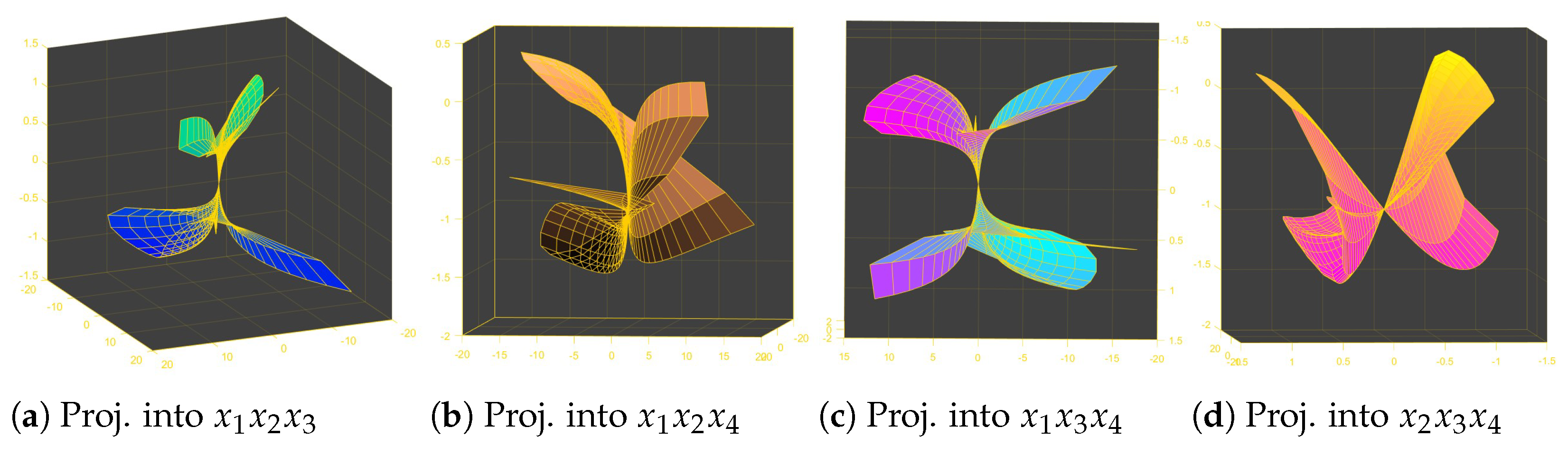
In Figure 1a, Figure 1b, Figure 1c, and Figure 1d, one can see the projections of the canal hypersurface (65) for $w=2$ into $x_1{x}_2{x}_3,$ $x_1{x}_2{x}_4,$ $x_1{x}_3{x}_4,$ and $x_2{x}_3{x}_4$−spaces, respectively.

From (37), (40), and (43) the Gaussian, mean, and principal curvatures of the canal hypersurface $X_1$ are obtained as

$$\left.\begin{array}{c}{K}_1(s,t,w)={\displaystyle \frac{24\left(t+w\right)}{s^2\left(3s\left(t+w\right)+\sqrt{3}\csc (t^2+w^2)\sec s\right)}},\hfill \\ H_1(s,t,w)=-{\displaystyle \frac{2\left(2+s(t+w)\sin (t^2+w^2)\cos s\left(\sqrt{3}-9s\left(t+w\right)\sin (t^2+w^2)\cos s\right)\right)}{3s\left(-1+3s^2{\left(t+w\right)}^2{\sin }^2(t^2+w^2){\cos }^{2}s\right)}},\hfill \\ {\left(p_1\right)}_1(s,t,w)={\displaystyle \frac{6(t+w)}{3s(t+w)+\sqrt{3}\sec s\csc (t^2+w^2)}},\hfill \\ {\left(p_2\right)}_1(s,t,w)={\left(p_3\right)}_1(s,t,w)={\displaystyle \frac{2}{s}}.\hfill \end{array}\right\}$$

(66)

In Figure 2a, Figure 2b, Figure 2c, and Figure 2d, one can see the graphics of the Gaussian, mean, first principal, and second–third principal curvature functions of the canal hypersurface $X_1$ for $w=2$, respectively.

If we use (64) and assume that $\mathfrak{h}(t,w)=t+w$ and $\mathfrak{f}(t,w)=t^2+w^2$ in the canal hypersurface $X_5(s,t,w)$ given as (29) formed as the envelope of a family of pseudo-hyperbolic hyperspheres with centers lying on the pseudo-null helix $\gamma \left(s\right)$ with Bishop vector fields in $E_1^4$, then $X_5(s,t,w)$ can be parameterized by

$$\begin{array}{ccc}& & X_5(s,t,w)\hfill \\ & & =\left(\begin{array}{c}{\displaystyle \frac{\left(\begin{array}{c}s{e}^{3s}\left(\begin{array}{c}25\cosh (t^2+w^2)\hfill \\ +3(t+w)\left(\begin{array}{c}\sqrt{5}\left(3\cos s+\sin s\right)\hfill \\ -5\left(\cos s-3\sin s\right)\sinh (t^2+w^2)\hfill \end{array}\right)\hfill \end{array}\right)\hfill \\ +(t+w)\cosh \left(3s\right)\left(4\sqrt{5}+45s(t+w)\cosh (t^2+w^2)\right)\hfill \end{array}\right)}{60\sqrt{2}(t+w)}},\hfill \\ {\displaystyle \frac{\left(\begin{array}{c}(t+w)\left(\begin{array}{c}4\sqrt{5}\sinh \left(3s\right)\hfill \\ +3s{e}^{3s}\left(\begin{array}{c}\sqrt{5}\left(3\cos s+\sin s\right)\hfill \\ -5\left(\cos s-3\sin s\right)\sinh (t^2+w^2)\hfill \end{array}\right)\hfill \end{array}\right)\hfill \\ +5s\cosh (t^2+w^2)\left(5e^{3s}+9{(t+w)}^2\sinh \left(3s\right)\right)\hfill \end{array}\right)}{60\sqrt{2}(t+w)}},\hfill \\ -{\displaystyle \frac{s-12\sin s+3\sqrt{5}s\left((t+w)\sin s\cosh (t^2+w^2)+\sinh (t^2+w^2)\right)}{4\sqrt{10}}},\hfill \\ {\displaystyle \frac{3(s-4\cos s)+\sqrt{5}s\left(3(t+w)\cos s\cosh (t^2+w^2)-\sinh (t^2+w^2)\right)}{4\sqrt{10}}}\hfill \end{array}\right),\hfill \end{array}$$

(67)

where the radius function has been taken as $r\left(s\right)={\displaystyle \frac{s}{2}}.$ Since $X_5(s,t,w)$ is obtained from (29), direct substitution verifies that $g(X_5(s,t,w)-\gamma \left(s\right),X_5(s,t,w)-\gamma \left(s\right))=-{\displaystyle \frac{s^2}{4}}=-r^2\left(s\right).$ Thus, (67) satisfies the defining pseudo-hyperbolic hypersphere condition.

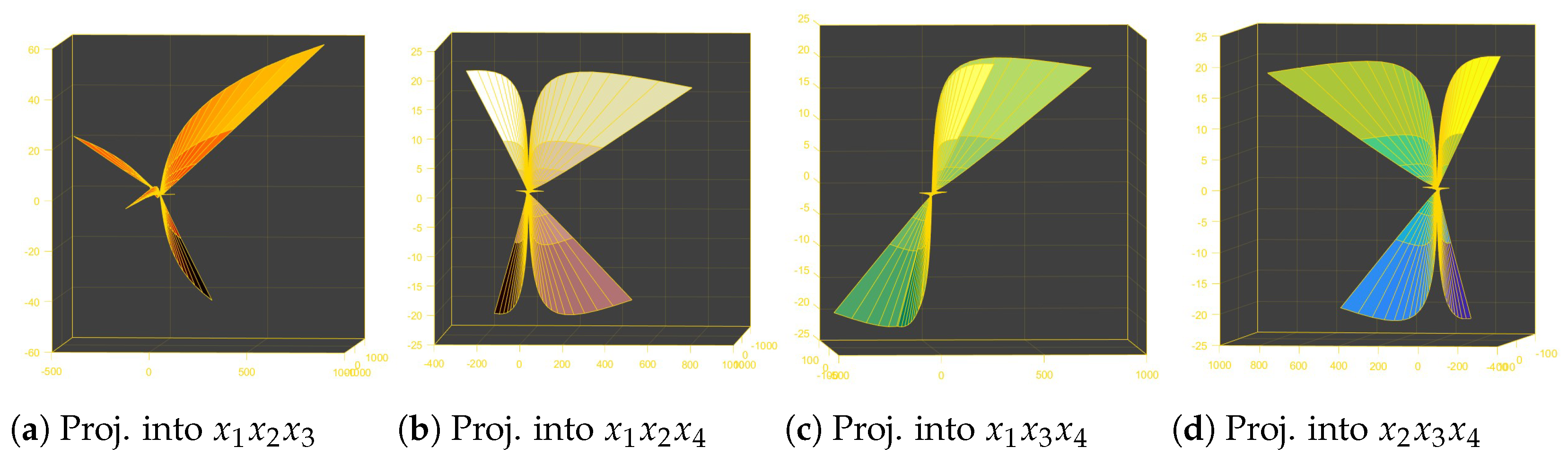
In Figure 3a, Figure 3b, Figure 3c, and Figure 3d, one can see the projections of the canal hypersurface (67) for $w=0.1$ into $x_1{x}_2{x}_3,$ $x_1{x}_2{x}_4,$ $x_1{x}_3{x}_4,$ and $x_2{x}_3{x}_4$−spaces, respectively.

From (44), (45), and (46) the Gaussian, mean, and principal curvatures of the canal hypersurface $X_5$ are obtained as

$$\left.\begin{array}{c}{K}_5(s,t,w)={\displaystyle \frac{24\left(t+w\right)}{s^2\left(3s(t+w)+\sqrt{5}\sec s\sec h(t^2+w^2)\right)}},\hfill \\ H_5(s,t,w)={\displaystyle \frac{-20+6s(t+w)\cos s\cosh (t^2+w^2)\left(-\sqrt{5}+9s(t+w)\cos s\cosh (t^2+w^2)\right)}{3s\left(-5+9s^2{(t+w)}^2{\cos }^{2}s{\cosh }^2(t^2+w^2)\right)}},\hfill \\ {\left(p_1\right)}_5(s,t,w)=-{\displaystyle \frac{6\left(t+w\right)}{3s(t+w)+\sqrt{5}\sec s\sec h(t^2+w^2)}},\hfill \\ {\left(p_2\right)}_5(s,t,w)={\left(p_3\right)}_5(s,t,w)=-{\displaystyle \frac{2}{s}}.\hfill \end{array}\right\}$$

(68)

In Figure 4a, Figure 4b, Figure 4c, and Figure 4d, one can see the graphics of the Gaussian, mean, first principal, and second–third principal curvature functions of the canal hypersurface $X_5$ for $w=0.1$, respectively.

The parametric expressions of the canal hypersurfaces $X_2(s,t,w)$, $X_3(s,t,w)$, and $X_4(s,t,w)$ along with their curvatures and figures can be obtained similarly.

6. Conclusions and Future Research

The present study introduces the canal hypersurfaces formed as the envelope of a family of pseudo-hyperspheres and pseudo-hyperbolic hyperspheres with centers lying on a pseudo-null curve with Bishop vector fields in four-dimensional Lorentz–Minkowski space. Parametric expressions for these canal hypersurfaces are obtained and geometric properties such as the Gaussian, mean, and principal curvatures are studied in detail. Furthermore, significant geometric characterizations are developed that provide a better understanding of these hypersurfaces.

Accordingly, our results allow for deeper study of hypersurfaces in Lorentz geometry while offering new avenues to investigate the properties of pseudo-null curves with Bishop frames in higher-dimensional spaces as well as the complex connections between geometry, curvature, and properties.

The study of these hypersurfaces is crucial for understanding how geometric structures behave, particularly in theoretical physics and general relativity.

In future research, the current results can be extended to more general families of hypersurfaces, particularly considering the geometric effects of higher-dimensional pseudo-null curves equipped with different structures. In this context, several open problems naturally arise, including the classification of canal hypersurfaces generated by pseudo-null curves in higher dimensions and the characterization of curvature properties under different frame choices. For example, to determine whether the hypersurfaces given in this study are Einstein or quasi-Einstein, the role of canal hypersurfaces in Einstein manifolds and spacetime geometry can be investigated. How frame choice and associated curvature functions affect these geometric properties remains a largely unexplored area. Additionally, investigating the stability and long-term behavior of canal hypersurfaces under geometric flows such as mean curvature flow and Ricci flow constitutes another challenging open direction for future research.

In conclusion, we think that the concepts developed in this study open up new avenues of application in fields where the geometry of hypersurfaces plays a fundamental role, including mathematical physics and differential geometry.

References

1. Altın, M.; Kazan, A. Rotational Hypersurfaces in Lorentz-Minkowski 4-Space. Hacet. J. Math. Stat. 2021, 50, 1409–1433. [Google Scholar] [CrossRef]
2. Altın, M.; Kazan, A.; Yoon, D.W. Canal Hypersurfaces generated by Non-Null Curves in Lorentz-Minkowski 4-Space. Bull. Korean Math. Soc. 2023, 60, 1299–1320. [Google Scholar] [CrossRef]
3. Bencheva, V.; Milousheva, V. Basic classes of timelike general rotational surfaces in the four-dimensional Minkowski space. Filomat 2023, 37, 8505–8519. [Google Scholar] [CrossRef]
4. Bencheva, V.; Milousheva, V. Timelike meridian surfaces of elliptic type in the Minkowski 4-space. arXiv 2025, arXiv:2504.00570. [Google Scholar] [CrossRef]
5. Güler, E.; Kişi, Ö. Dini-type helicoidal hypersurfaces with timelike axis in Minkowski 4-space E 1 4 . Mathematics 2019, 7, 205. [Google Scholar] [CrossRef]
6. Izumiya, S.; Fuster, M.D.C.R.; Saji, K. Flat lightlike hypersurfaces in Lorentz-Minkowski 4-space. J. Geom. Phys. 2009, 59, 1528–1546. [Google Scholar] [CrossRef]
7. Do Carmo, M.P. Differential Geometry of Curves and Surfaces; Prentice-Hall: Englewood Cliffs, NJ, USA, 1976; ISBN 0-13-212589-7. [Google Scholar]
8. Aslan, S.; Yaylı, Y. Canal surfaces with quaternions. Adv. Appl. Clifford Algebr. 2016, 26, 31–38. [Google Scholar] [CrossRef]
9. Bulca, B.; Aslan, K.; Bayram, B.; Öztürk, G. Canal surfaces in 4-dimensional Euclidean space. Int. J. Optim. Control Theor. Appl. 2017, 7, 83–89. [Google Scholar] [CrossRef]
10. Garcia, R.; Llibre, J.; Sotomayor, J. Lines of principal curvature on canal surfaces in R 3 . An. Acad. Bras. Cienc. 2006, 78, 405–415. [Google Scholar] [CrossRef] [PubMed]
11. Karacan, M.K.; Es, H.; Yaylı, Y. Singular points of tubular surfaces in Minkowski 3-space. Sarajev. J. Math. 2006, 2, 73–82. [Google Scholar] [CrossRef]
12. Kazan, A.; Altın, M.; Yoon, D.W. Geometric characterizations of canal hypersurfaces in Euclidean spaces. Filomat 2023, 37, 5909–5920. [Google Scholar] [CrossRef]
13. Xu, Z.; Feng, R.; Sun, J.-G. Analytic and algebraic properties of canal surfaces. J. Comput. Appl. Math. 2006, 195, 220–228. [Google Scholar] [CrossRef]
14. Ahmadzadeh, S.R.; Rana, M.A.; Chernova, S. Generalized cylinders for learning, reproduction, generalization, and refinement of robot skills. Robot. Sci. Syst. 2017, 1, 1–10. [Google Scholar] [CrossRef]
15. Ambrosini, P.; Ruijters, D.; Niessen, W.J.; Moelker, A.; van Walsum, T. Fully automatic and real-time catheter segmentation in x-ray fluoroscopy. In International Conference on Medical Image Computing and Computer-Assisted Intervention; Springer: Cham, Switzerland, 2017; pp. 577–585. [Google Scholar] [CrossRef]
16. Nour, M.A.; Hussain, M.M. A review of the real-time monitoring of fluid-properties in tubular architectures for industrial applications. Sensor 2020, 20, 3907. [Google Scholar] [CrossRef]
17. Nunez-Valdes, J.; Almagro, I.O. Canal surfaces and its application to the CAGD. Am. J. Eng. Res. (AJER) 2021, 10, 19–31. [Google Scholar]
18. Shen, C.; Gao, B.; Lv, K.; Yao, H. Computational fluid dynamics in root canal irrigation. Int. J. Numer. Methods Biomed. Eng. 2023, 39, e3738. [Google Scholar] [CrossRef] [PubMed]
19. Camcı, Ç.; Uçum, A.; İlarslan, K. New results concerning Cartan null and pseudo null curves in Minkowski 3-space. J. Geom. 2023, 114, 15. [Google Scholar] [CrossRef]
20. Çimdiker Aslan, M. Geometry of the non-degenerate Hasimoto-like surfaces for the classification of pseudo-null curve evolution using Darboux triad. Int. J. Geom. Methods Mod. Phys. 2025, 22, 2550120. [Google Scholar] [CrossRef]
21. Erdoğdu, M. Electromagnetic waves along pseudo null curves in Minkowski space. Heliyon 2022, 8, e10061. [Google Scholar] [CrossRef]
22. Ertuğ Gürbüz, N. The pseudo-null geometric phase along optical fiber. Int. J. Geom. Methods Mod. Phys. 2021, 18, 2150230. [Google Scholar] [CrossRef]
23. Ertuğ Gürbüz, N. The variation of the electric field along optic fiber for null Cartan and pseudo-null frames. Int. J. Geom. Methods Mod. Phys. 2021, 18, 2150122. [Google Scholar] [CrossRef]
24. Ünlütürk, Y.; Ünal, D. A new glimpse into the directional curves associated with a pseudo-null curve via Bishop frame. Waves Random Complex Media 2025, 35, 2083–2094. [Google Scholar] [CrossRef]
25. Yavuz, A.; Erdoğdu, M. Congruence of degenerate surface along pseudo null curve and Landau-Lifshitz equation. J. Geom. Phys. 2022, 178, 104553. [Google Scholar] [CrossRef]
26. O’Neill, B. Semi-Riemannian Geometry with Applications to Relativity; Academic Press: New York, NY, USA, 1983. [Google Scholar]
27. Djordjevic, J.; Nesovic, E. On Bishop frame of a pseudo null curve in Minkowski space-time. Turk. J. Math. 2020, 44, 870–882. [Google Scholar] [CrossRef]
28. Walrave, J. Curves and Surfaces in Minkowski Space. Doctoral Thesis, KU Leuven, Faculty of Science, Leuven, Brussels, 1995. [Google Scholar]
29. Aydın, M.E.; Mihai, I. On certain surfaces in the isotropic 4-space. Math. Commun. 2017, 22, 41–51. [Google Scholar]
30. Güler, E. Helical Hypersurfaces in Minkowski Geometry E 1 4 . Symmetry 2020, 12, 1206. [Google Scholar] [CrossRef]
31. Kazan, A. Canal Hypersurfaces according to one of the Extended Darboux Frame Field in Euclidean 4-Space. Therm. Sci. 2022, 26, 3029–3041. [Google Scholar] [CrossRef]
32. Kişi, İ.; Öztürk, G.; Arslan, K. A new type of canal surface in Euclidean 4-space E4. Sak. Univ. J. Sci. 2019, 23, 801–809. [Google Scholar] [CrossRef][Green Version]
33. Lee, J.M. Riemannian Manifolds-An Introduction to Curvature; Springer: New York, NY, USA, 1997. [Google Scholar]
Figure 1. The projections of the canal hypersurface in (65).
Symmetry 18 00935 g001
Figure 2. The graphics of the curvature functions in (66).
Symmetry 18 00935 g002
Figure 3. The projections of the canal hypersurface in (67).
Symmetry 18 00935 g003
Figure 4. The graphics of the curvature functions in (68).
Symmetry 18 00935 g004
Disclaimer/Publisher’s Note: The statements, opinions and data contained in all publications are solely those of the individual author(s) and contributor(s) and not of MDPI and/or the editor(s). MDPI and/or the editor(s) disclaim responsibility for any injury to people or property resulting from any ideas, methods, instructions or products referred to in the content.