Tensor Completion via Linear Combination of Nuclear Norms

Abstract

Tensor completion is commonly formulated by minimizing a convex combination of nuclear norms of mode-wise unfolding matrices. Although effective, the non-negative weight constraint can limit the flexibility of mode balancing, especially when different modes contribute unequally to the reconstruction. In this paper, we propose a tensor completion model based on a linear combination of nuclear norms, where the weights are allowed to take signed values under a normalization constraint. To implement this model, we develop an ADMM-based algorithm, termed FlexHaLRTC, which extends the standard singular value thresholding update to handle both shrinkage for positive weights and expansion for negative weights. Experiments on color image inpainting and video completion show that the proposed method achieves competitive PSNR, SSIM, and RSE results, with more noticeable gains in high-missing-rate settings.

1. Introduction

Tensor completion aims to recover missing entries of partially observed multi-dimensional data by exploiting structural regularity across different modes [1,2,3,4,5,6,7,8]. Because tensors preserve multi-way relationships that are often lost under matrix flattening, tensor-based models have been widely used in image restoration, video processing, recommendation systems, and other applications involving high-dimensional structured data [1,9,10,11,12,13,14,15,16,17]. In many practical scenarios, however, tensor observations are incomplete due to occlusion, transmission errors, sensing limitations, or data corruption [1,18,19], making reliable recovery of missing entries a central problem.

A common modeling assumption is that the underlying tensor admits approximately low-rank structures across its mode unfoldings. Under this assumption, tensor completion can be viewed as a rank minimization problem constrained by the observed entries [20]. Since direct tensor-rank minimization is NP-hard [21], practical methods typically replace rank with tractable surrogates, often employing advanced optimization algorithms such as accelerated gradient or coordinate descent methods [22,23,24]. One of the most widely used formulations minimizes a weighted sum of nuclear norms of the unfolding matrices [11,13,25], leading to the convex combination model

$$\underset{\mathcal{X}}{\min }{\displaystyle \sum _{i=1}^n}{\alpha }_i{\parallel {\mathcal{X}}_{\left(i\right)}\parallel }_{*}\mathrm{s}.\mathrm{t}.{\mathcal{X}}_{\mathsf{\Omega }}={\mathcal{T}}_{\mathsf{\Omega }},{\alpha }_i\ge 0,$$

(1)

where ${\alpha }_i\ge 0$ and ${\sum }_{i=1}^n{\alpha }_i=1$. This formulation has shown good empirical performance and underlies several influential tensor completion methods, including high-accuracy low-rank tensor completion (HaLRTC) [1].

Despite its practical success, the convex-combination formulation imposes a restrictive weighting rule: all mode weights must be non-negative. This requirement is natural from the convex-analysis viewpoint, but it may also limit the flexibility with which different tensor modes are balanced in reconstruction. In particular, when different modes exhibit heterogeneous structural roles, a purely non-negative weighting scheme may be too rigid to express mode-dependent emphasis or relaxation. Motivated by this observation, we study whether allowing signed weights can provide a useful extension of unfolding-based nuclear-norm regularization.

Based on this idea, we consider the following linear combination model:

$$\underset{\mathcal{X}}{\min }{\displaystyle \sum _{i=1}^n}{\alpha }_i{\parallel {\mathcal{X}}_{\left(i\right)}\parallel }_{*}\mathrm{s}.\mathrm{t}.{\mathcal{X}}_{\mathsf{\Omega }}={\mathcal{T}}_{\mathsf{\Omega }},{\alpha }_i\in \mathbb{R},{\displaystyle \sum _{i=1}^n}{\alpha }_i=1.$$

(2)

where ${\alpha }_i\in \mathbb{R}$ are predetermined weights satisfying ${\sum }_{i=1}^n{\alpha }_i=1$. Relative to the standard convex combination, this model enlarges the admissible weighting space while retaining the same unfolding-based nuclear-norm structure. To solve it numerically, we build on the ADMM framework of HaLRTC and introduce an extended singular value thresholding-style update that handles both positive and negative weights.

Our main contributions are threefold:

• Model formulation. We extend the standard convex-combination weighting rule to a signed linear-combination framework for unfolding-based tensor nuclear norms.
• Algorithm design. We develop an ADMM-based algorithm, FlexHaLRTC, with an extended SVT-style update to implement the signed-weight model.
• Empirical evaluation. We report competitive results on image inpainting and video completion, with more noticeable gains in several high-missing-rate settings.

The remainder of this paper is organized as follows. Section 2 introduces the notation and preliminaries. Section 3 presents our FlexHaLRTC (flexible high-accuracy low-rank tensor completion) algorithm, an ADMM-based method for solving the proposed linear combination model. Section 4 provides experimental results on color image inpainting. Section 5 extends the evaluation to video completion tasks. Section 6 concludes with discussions and future directions.

2. Notation and Preliminaries

We follow standard mathematical conventions. Uppercase letters (e.g., X) denote matrices, lowercase letters (e.g., $x_{ij}$) denote scalars, and calligraphic letters (e.g., $\mathcal{X}$) denote tensors. For a matrix $X\in {\mathbb{R}}^{m\times n}$, the Frobenius norm is defined as ${\parallel X\parallel }_F:=\sqrt{{\sum }_{i,j}{x}_{ij}^2}$, and the nuclear norm as ${\parallel X\parallel }_{*}:={\sum }_i{\sigma }_i\left(X\right)$, where ${\sigma }_i\left(X\right)$ denotes the i-th largest singular value. The nuclear norm is the tightest convex relaxation of the matrix rank function [26,27]. The singular value decomposition (SVD) of X is denoted as $X=U\Sigma V^T$, where $U\in {\mathbb{R}}^{m\times r}$ and $V\in {\mathbb{R}}^{n\times r}$ have orthonormal columns, $\Sigma =\mathrm{diag}({\sigma }_1,\dots ,{\sigma }_r)$ with ${\sigma }_1\ge {\sigma }_2\ge \cdots \ge {\sigma }_r>0$, and $r=\mathrm{rank}\left(X\right)$. For an n-th order tensor $\mathcal{X}\in {\mathbb{R}}^{I_1\times I_2\times \cdots \times I_n}$, a mode-i fiber is a vector obtained by fixing all indices except the i-th one, and the mode-i unfolding ${\mathcal{X}}_{\left(i\right)}\in {\mathbb{R}}^{I_i\times {\prod }_{j\ne i}{I}_j}$ is a matrix formed by arranging all mode-i fibers as its columns. The Tucker rank of $\mathcal{X}$ is the tuple $(r_1,r_2,\dots ,r_n)$ where $r_i=\mathrm{rank}\left({\mathcal{X}}_{\left(i\right)}\right)$. When we refer to $\mathrm{rank}\left(\mathcal{X}\right)$ in optimization problems, it denotes the Tucker rank unless otherwise specified. The Frobenius norm of tensor $\mathcal{X}$ is defined as ${\parallel \mathcal{X}\parallel }_F:=\sqrt{{\sum }_{i_1,\dots ,i_n}{\mathcal{X}}_{i_1,\dots ,i_n}^2}$, which satisfies ${\parallel \mathcal{X}\parallel }_F={\parallel {\mathcal{X}}_{\left(i\right)}\parallel }_F$ for all i.

For the tensor completion problem, $\mathsf{\Omega }\subseteq \{1,\dots ,I_1\}\times \cdots \times \{1,\dots ,I_n\}$ denotes the set of indices of observed entries, ${\mathcal{X}}_{\mathsf{\Omega }}$ denotes the restriction of tensor $\mathcal{X}$ to $\mathsf{\Omega }$, and ${\mathcal{T}}_{\mathsf{\Omega }}$ denotes the observed values. Given weight parameters ${\alpha }_1,\dots ,{\alpha }_n$, a convex combination requires ${\alpha }_i\ge 0$ and ${\sum }_{i=1}^n{\alpha }_i=1$, while a linear combination allows ${\alpha }_i\in \mathbb{R}$ with the normalization constraint ${\sum }_{i=1}^n{\alpha }_i=1$. In the ADMM algorithm, $M_i^{\left(k\right)}$ denotes the auxiliary matrix variable for mode i at iteration k, $Y_i^{\left(k\right)}$ denotes the Lagrange multiplier matrix, and $\rho >0$ is the penalty parameter.

The singular value thresholding (SVT) operator [28] serves as the proximal operator of the nuclear norm. For a matrix A with SVD $A=U\Sigma V^T$, where $\Sigma =\mathrm{diag}({\sigma }_1,\dots ,{\sigma }_r)$ and threshold $\tau \ge 0$, the standard SVT is ${\mathcal{D}}_{\tau }\left(A\right)=U\mathrm{diag}\left(\max ({\sigma }_i-\tau ,0)\right)V^T$, which solves $\arg {\min }_X{\displaystyle \frac{1}{2}}{\parallel X-A\parallel }_F^2+\tau {\parallel X\parallel }_{*}$ and promotes low-rank structure through soft thresholding. To accommodate negative weights, we introduce an extended SVT-style update for negative thresholds: for $\tau <0$, we define ${\mathcal{D}}_{\tau }\left(A\right)=U\mathrm{diag}({\sigma }_i+\left|\tau \right|)V^T$. This extension should be viewed as an algorithmic rule that symmetrically expands singular values when the corresponding weight is negative, rather than as the proximal operator of a convex penalty. The unified definition is

$${\mathcal{D}}_{\tau }\left(A\right)=\left\{\begin{array}{cc}U\mathrm{diag}\left(\max ({\sigma }_i-\tau ,0)\right)V^T,\hfill & \mathrm{if}\tau \ge 0,\hfill \\ U\mathrm{diag}({\sigma }_i+\left|\tau \right|)V^T,\hfill & \mathrm{if}\tau <0.\hfill \end{array}\right.$$

(3)

In our ADMM framework, the threshold for mode i is ${\tau }_i={\alpha }_i/\rho$. Consequently, when ${\alpha }_i>0$, ${\mathcal{D}}_{{\tau }_i}$ induces rank reduction via shrinkage; when ${\alpha }_i<0$, it induces rank enhancement via expansion; when ${\alpha }_i=0$, no thresholding is applied.

3. Optimization Algorithm

As discussed in the previous section, the linear combination model is intended to relax the expressiveness limitations of the traditional convex combination framework by allowing the weights ${\alpha }_i$ to take arbitrary real values, subject only to the normalization constraint ${\sum }_{i=1}^n{\alpha }_i=1$. This added flexibility also introduces additional challenges in the optimization procedure.

To efficiently solve the resulting optimization problem, we adopt an Alternating Direction Method of Multipliers (ADMM) framework [29], which is based on the successful HaLRTC algorithm. The ADMM framework is well suited to this problem because it decomposes the objective into simpler subproblems that can be handled efficiently. Our algorithm follows the overall structure of HaLRTC, with the main modification being the singular value thresholding (SVT) step, which is extended to accommodate both positive and negative weights.

3.1. HaLRTC ADMM Framework

The HaLRTC algorithm solves the convex combination tensor completion problem using ADMM. The optimization problem is reformulated by introducing auxiliary variables $M_i\in {\mathbb{R}}^{I_i\times {\prod }_{j\ne i}{I}_j}$ for each mode i, representing the low-rank approximations of the mode-unfolding matrices:

$$\underset{\mathcal{X},{\left\{M_i\right\}}_{i=1}^n}{\min }{\displaystyle \sum _{i=1}^n}{\alpha }_i{\parallel M_i\parallel }_{*}\mathrm{s}.\mathrm{t}.\left\{\begin{array}{cc}{\mathcal{X}}_{\left(i\right)}=M_i,\hfill & i=1,\dots ,n\hfill \\ {\mathcal{X}}_{\mathsf{\Omega }}={\mathcal{T}}_{\mathsf{\Omega }}\hfill & \end{array}\right.,$$

(4)

where ${\alpha }_i\ge 0$ and ${\sum }_{i=1}^n{\alpha }_i=1$. The augmented Lagrangian function is

$$\begin{array}{cc}\hfill L_{\rho }(\mathcal{X},M_1,\dots ,M_n,Y_1,\dots ,Y_n)& \\ \hfill =& {\displaystyle \sum _{i=1}^n}{\alpha }_i\parallel M_i{\parallel }_{*}+{\displaystyle \sum _{i=1}^n}〈Y_i,{\mathcal{X}}_{\left(i\right)}-M_i〉+{\displaystyle \frac{\rho }{2}}{\displaystyle \sum _{i=1}^n}{\parallel {\mathcal{X}}_{\left(i\right)}-M_i\parallel }_F^2.\hfill \end{array}$$

(5)

The ADMM algorithm iteratively updates the variables as follows:

• Update $M_i^{(k+1)}$ for $i=1,\dots ,n$:

This step involves minimizing the augmented Lagrangian with respect to $M_i$:

$$\underset{M_i}{\min }{\alpha }_i{\parallel M_i\parallel }_{*}+{\displaystyle \frac{\rho }{2}}{∥{\mathcal{X}}_{\left(i\right)}^{\left(k\right)}-M_i+{\rho }^{-1}{Y}_i^{\left(k\right)}∥}_F^2.$$

(6)

The solution is obtained via the singular value thresholding (SVT) operator:

$$M_i^{(k+1)}={\mathcal{D}}_{{\tau }_i}\left({\mathcal{X}}_{\left(i\right)}^{\left(k\right)}+{\rho }^{-1}{Y}_i^{\left(k\right)}\right),$$

(7)

where ${\tau }_i={\alpha }_i/\rho$. Since ${\alpha }_i\ge 0$ in HaLRTC, the threshold ${\tau }_i$ is non-negative, and the SVT operator shrinks singular values via soft thresholding.

• Update ${\mathcal{X}}^{(k+1)}$:

This step minimizes the augmented Lagrangian with respect to $\mathcal{X}$:

$$\underset{\mathcal{X}:{\mathcal{X}}_{\mathsf{\Omega }}={\mathcal{T}}_{\mathsf{\Omega }}}{\min }{\displaystyle \sum _{i=1}^n}\parallel {\mathcal{X}}_{\left(i\right)}-\left(M_i^{(k+1)}-{\rho }^{-1}{Y}_i^{\left(k\right)}\right){\parallel }_F^2.$$

(8)

The solution is

$${\mathcal{X}}^{(k+1)}={\mathcal{P}}_{\mathsf{\Omega }}\left(\mathcal{T}\right)+{\mathcal{P}}_{{\mathsf{\Omega }}^c}\left({\displaystyle \frac{1}{n}}{\displaystyle \sum _{i=1}^n}{\mathcal{Q}}_i^{(k+1)}\right),$$

(9)

where ${\mathcal{Q}}_i^{(k+1)}={\mathrm{fold}}_i(M_i^{(k+1)}-{\rho }^{-1}{Y}_i^{\left(k\right)})$ denotes the tensor reconstructed by folding the matrix back along mode i.

• Update $Y_i^{(k+1)}$ for $i=1,\dots ,n$:

The Lagrange multipliers are updated using

$$Y_i^{(k+1)}=Y_i^{\left(k\right)}+\rho \left({\mathcal{X}}_{\left(i\right)}^{(k+1)}-M_i^{(k+1)}\right).$$

(10)

3.2. Extension to Linear Combination

We now extend the HaLRTC framework to allow arbitrary real-valued weights ${\alpha }_i\in \mathbb{R}$ subject to the constraint ${\sum }_{i=1}^n{\alpha }_i=1$. We refer to this extended algorithm as FlexHaLRTC to emphasize its flexibility in handling both positive and negative weights. Because the signed weights relax the standard non-negativity constraint, the resulting objective should be viewed as a heuristic extension of the original convex-combination model rather than a standard convex optimization problem. The key modification lies in the singular value thresholding step, where the threshold ${\tau }_i={\alpha }_i/\rho$ can now be negative.

Following the unified SVT definition from Section 2, the $M_i$ update becomes

$$M_i^{(k+1)}={\mathcal{D}}_{{\tau }_i}\left({\mathcal{X}}_{\left(i\right)}^{\left(k\right)}+{\rho }^{-1}{Y}_i^{\left(k\right)}\right),$$

(11)

where the extended SVT operator is defined as

$${\mathcal{D}}_{\tau }\left(A\right)=\left\{\begin{array}{cc}U\mathrm{diag}\left(\max ({\sigma }_i-\tau ,0)\right)V^T,\hfill & \mathrm{if}\tau \ge 0,\hfill \\ U\mathrm{diag}({\sigma }_i+\left|\tau \right|)V^T,\hfill & \mathrm{if}\tau <0,\hfill \end{array}\right.$$

(12)

and $A=U\mathrm{diag}({\sigma }_1,\dots ,{\sigma }_r)V^T$ is the singular value decomposition of A.

When ${\alpha }_i\ge 0$ (positive weight), we have ${\tau }_i\ge 0$, and the SVT operator performs soft thresholding. The element-wise transformation is

$${\tilde{\sigma }}_j=\max ({\sigma }_j-{\tau }_i,0)=\left\{\begin{array}{cc}{\sigma }_j-{\tau }_i,\hfill & \mathrm{if}{\sigma }_j>{\tau }_i,\hfill \\ 0,\hfill & \mathrm{if}{\sigma }_j\le {\tau }_i.\hfill \end{array}\right.$$

(13)

This shrinkage operation promotes low-rank structures by eliminating small singular values and reducing the magnitude of larger ones.

When ${\alpha }_i<0$ (negative weight), we have ${\tau }_i<0$, and the SVT operator expands the singular values. The element-wise transformation is

$${\tilde{\sigma }}_j={\sigma }_j+\left|{\tau }_i\right|,\forall j.$$

(14)

Since ${\tau }_i<0$, we have $|{\tau }_i|=-{\tau }_i$; thus, this operation uniformly increases all singular values by $|{\tau }_i|$. In algorithmic terms, this expansion increases the influence of mode i in the reconstruction and can counterbalance over-aggressive low-rank shrinkage when the data contains a richer structure than a purely low-rank model can capture.

The negative weights can therefore be interpreted as a flexible way to modulate the relative influence of different tensor modes, rather than enforcing low-rank regularization uniformly across all unfoldings. This interpretation is particularly reasonable for RGB data, where the color mode has only three channels and is structurally different from the spatial modes; using a slightly negative weight helps avoid over-constraining inter-channel variation while preserving the dominant spatial low-rank structure. A heuristic interpretation of this extended SVT update is provided in Appendix A.

The mathematical formulation for our linear combination model is identical to (4), except that the weights ${\alpha }_i$ are no longer constrained to be non-negative. The update rules for $\mathcal{X}$ and $Y_i$ remain the same as in HaLRTC, with only the $M_i$ update step modified to handle negative thresholds through the extended SVT-style update.

3.3. Weight Parameter Selection

In the FlexHaLRTC framework, the weights ${\left\{{\alpha }_i\right\}}_{i=1}^n$ are treated as hyperparameters. While theoretical guidelines for optimal weight selection remain an open research question, we adopt an empirical approach. The weights can be chosen based on prior knowledge about the data or tuned on a validation set. For instance, if one mode is known to be more corrupted or less structured, it could be assigned a negative or smaller positive weight. In practice, we found that a mild negative weight on the color mode, such as ${\alpha }_3=-0.1$ in the image experiments, is more stable than using a large negative value. This provides a mechanism for mode-dependent regularization.

In our experiments (Section 4), we demonstrate this process by conducting a grid search on a validation image to identify an effective weight configuration, which is then applied to the entire test set. The complete procedure of our proposed method is summarized in Algorithm 1.

Algorithm 1 FlexHaLRTC algorithm.

Require: Observed entries ${\mathcal{T}}_{\mathsf{\Omega }}$, observation index set $\mathsf{\Omega }$, weights ${\left\{{\alpha }_i\right\}}_{i=1}^n$ with ${\sum }_{i=1}^n{\alpha }_i=1$

(may be negative), penalty parameter $\rho >0$, maximum iterations K

Ensure: Completed tensor $\mathcal{X}$

1: Initialize $Y_i=0$, $M_i=0$ for $i=1,\dots ,n$   2: Initialize ${\mathcal{X}}_{\mathsf{\Omega }}={\mathcal{T}}_{\mathsf{\Omega }}$ and ${\mathcal{X}}_{{\mathsf{\Omega }}^c}=0$   3: for $k=1$ to K do   4:       for $i=1$ to n do   5:             $Q_i\leftarrow {\mathrm{unfold}}_i\left(\mathcal{X}\right)+Y_i/\rho$   6:             Compute the SVD $Q_i=U\Sigma V^T$ and let $\sigma =\mathrm{diag}(\Sigma )$   7:             ${\tau }_i\leftarrow {\alpha }_i/\rho$   8:             if ${\tau }_i\ge 0$ then   9:                   $M_i\leftarrow U\mathrm{diag}\left(\max (\sigma -{\tau }_i,0)\right)V^T$ 10:             else 11:                   $M_i\leftarrow U\mathrm{diag}(\sigma + |{\tau }_i\left|\right)V^T$ 12:             end if 13:       end for 14:       ${\mathcal{X}}_{{\mathsf{\Omega }}^c}\leftarrow {\left({\displaystyle \frac{1}{n}}{\sum }_{i=1}^n{\mathrm{fold}}_i(M_i-{\rho }^{-1}{Y}_i)\right)}_{{\mathsf{\Omega }}^c}$ 15:       ${\mathcal{X}}_{\mathsf{\Omega }}\leftarrow {\mathcal{T}}_{\mathsf{\Omega }}$ 16:       for $i=1$ to n do 17:             $Y_i\leftarrow Y_i+\rho ({\mathrm{unfold}}_i\left(\mathcal{X}\right)-M_i)$ 18:       end for 19: end for 20: return  $\mathcal{X}$

FlexHaLRTC extends the traditional ADMM framework by allowing signed weights in the unfolding-based regularization term and by incorporating the corresponding extended SVT-style update. This generalization provides a more flexible mode-dependent regularization mechanism while retaining a simple implementation. In practice, the algorithm exhibits stable empirical behavior under moderate negative weights for the parameter ranges considered in our experiments.

4. Experimental Results

4.1. Experimental Configuration and Implementation Details

To ensure reproducibility and facilitate a fair comparison, we provide comprehensive implementation details for all experiments conducted in this study.

4.1.1. Hardware and Software Environment

All experiments were conducted on a laptop with an Intel Core i5-10200H CPU and 16 GB RAM running Windows 11 (64-bit). We used MATLAB R2021a and Python 3.8.10 (NumPy 1.21.2, SciPy 1.7.1, PyTorch 1.9.0, OpenCV 4.5.3, Matplotlib 3.4.3, scikit-image 0.18.3, Pillow 8.3.1). The seven test images (Airplane, Baboon, Cloudy, House, Panda, Peppers, and Parrot) and the Foreman/Akiyo video sequences are standard public benchmarks widely used in the image and video processing community (e.g., from the USC-SIPI Image Database and other open research repositories). These datasets are publicly available for academic research purposes.

4.1.2. Algorithm-Specific Hyperparameters

For a fair comparison, we used the parameter settings recommended in the original publications for all baselines.

For the proposed FlexHaLRTC and the baseline HaLRTC algorithms, we utilized a fixed-iteration stopping criterion. Specifically, we set the penalty parameter $\rho ={10}^{-5}$ and fixed the maximum iterations at $K=150$. HaLRTC utilized its default uniform weights $\mathit{\alpha }=[1/3,1/3,1/3]$. Conversely, for FlexHaLRTC, the weight configuration $\mathit{\alpha }=[0.6,0.5,-0.1]$ was determined via a grid search on validation data, where the negative weight on the color mode enables more flexible inter-channel correlation modeling.

For other competing methods, we strictly followed the default parameter settings optimized in their original publications. Specifically, SILRTC [1] was restricted to $K=150$ with $\mathit{\alpha }=[0.2,0.7,0.1]$. TNN [13] and WSTNN [30] utilized adaptive penalty updates with their default tolerance $ϵ={10}^{-5}$. Lp-TNN [31] was set with truncation parameter $p=0.5$ and truncation rank $r=10$. Both tensor ring methods (NTRC and FANTRC [32]) employed regularization parameter $\lambda =28$ with $K=1000$.

4.2. Color Image Restoration Under Random Missing Patterns

4.2.1. Test Dataset and Evaluation Metrics

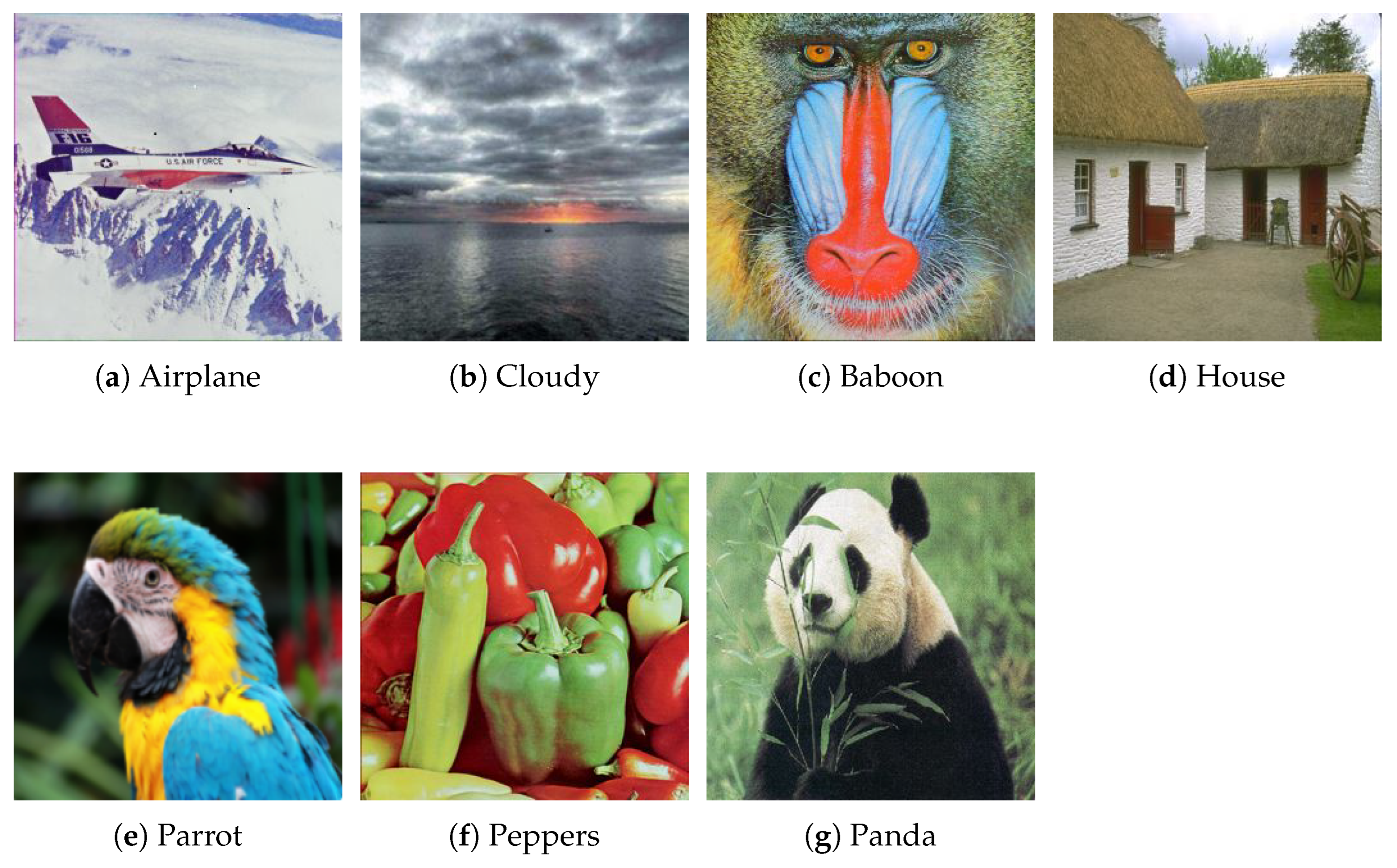
To evaluate our algorithm under random pixel missing scenarios, we selected seven representative $256\times 256$ RGB images (Figure 1) covering natural scenes and complex textures. We simulated uniform random pixel loss from 30% to 90% and compared FlexHaLRTC with seven state-of-the-art tensor completion algorithms (HaLRTC [1], SILRTC [1], TNN [13], WSTNN [30], Lp-TNN [31], NTRC [32], and FANTRC [32]).

The restoration performance was quantitatively evaluated using PSNR, SSIM, and RSE. The peak signal-to-noise ratio (PSNR) is defined as

$$\mathrm{PSNR}=10·{\log }_{10}\left({\displaystyle \frac{{\mathrm{MAX}}^2}{\mathrm{MSE}}}\right),$$

(15)

where MAX is the maximum possible pixel value (e.g., 255 for 8-bit images) and $\mathrm{MSE}={\displaystyle \frac{1}{mn}}{\sum }_{i,j}{(X_{ij}-{\widehat{X}}_{ij})}^2$ is the mean squared error between the original image X and the reconstructed image $\widehat{X}$. The structural similarity index (SSIM) is defined as

$$\mathrm{SSIM}(X,\widehat{X})={\displaystyle \frac{(2{\mu }_X{\mu }_{\widehat{X}}+c_1)(2{\sigma }_{X\widehat{X}}+c_2)}{({\mu }_X^2+{\mu }_{\widehat{X}}^2+c_1)({\sigma }_X^2+{\sigma }_{\widehat{X}}^2+c_2)}},$$

(16)

where ${\mu }_X$ and ${\mu }_{\widehat{X}}$ are the mean values, ${\sigma }_X^2$ and ${\sigma }_{\widehat{X}}^2$ are the variances, ${\sigma }_{X\widehat{X}}$ is the covariance, and $c_1$ and $c_2$ are small constants for numerical stability. The relative squared error (RSE) is defined as

$$\mathrm{RSE}={\displaystyle \frac{\parallel \mathcal{X}-\widehat{\mathcal{X}}{\parallel }_F}{{\parallel \mathcal{X}\parallel }_F}},$$

(17)

where $\mathcal{X}$ and $\widehat{\mathcal{X}}$ denote the original and reconstructed tensors, respectively. Higher PSNR and SSIM values indicate better reconstruction quality, while lower RSE values are preferred.

4.2.2. Empirical Convergence Analysis

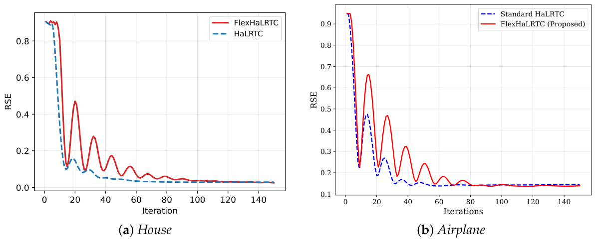
Due to the introduction of negative weights in the proposed linear-combination model, establishing a rigorous theoretical convergence proof is non-trivial. Therefore, we provide an empirical convergence study on two representative images, House and Airplane, under a 90% missing rate. We compare FlexHaLRTC with the standard HaLRTC using the same observation masks and report the relative squared error (RSE) along the iterations.

As shown in Figure 2, both methods exhibit stable empirical convergence behavior across different image contents. The RSE curves for both images gradually flatten after approximately 120 iterations. Notably, FlexHaLRTC attains a lower final reconstruction error than HaLRTC in both cases, with final RSE values reaching steady states significantly earlier. These results provide empirical evidence that the proposed algorithm remains stable and robust in practice despite the use of moderate negative weights.

It is worth noting that while the introduction of negative weights provides significant flexibility and performance gains, it also poses a non-trivial challenge for a rigorous theoretical convergence proof, as the objective function may deviate from standard convexity. However, the comprehensive empirical studies conducted on various images consistently demonstrate that FlexHaLRTC maintains a stable and monotonic convergence behavior in practice. We regard the formal mathematical derivation of the convergence boundaries for this flexible weighting scheme as a significant direction for our future research.

4.2.3. Sensitivity Analysis of Weight Parameter ${\alpha }_3$

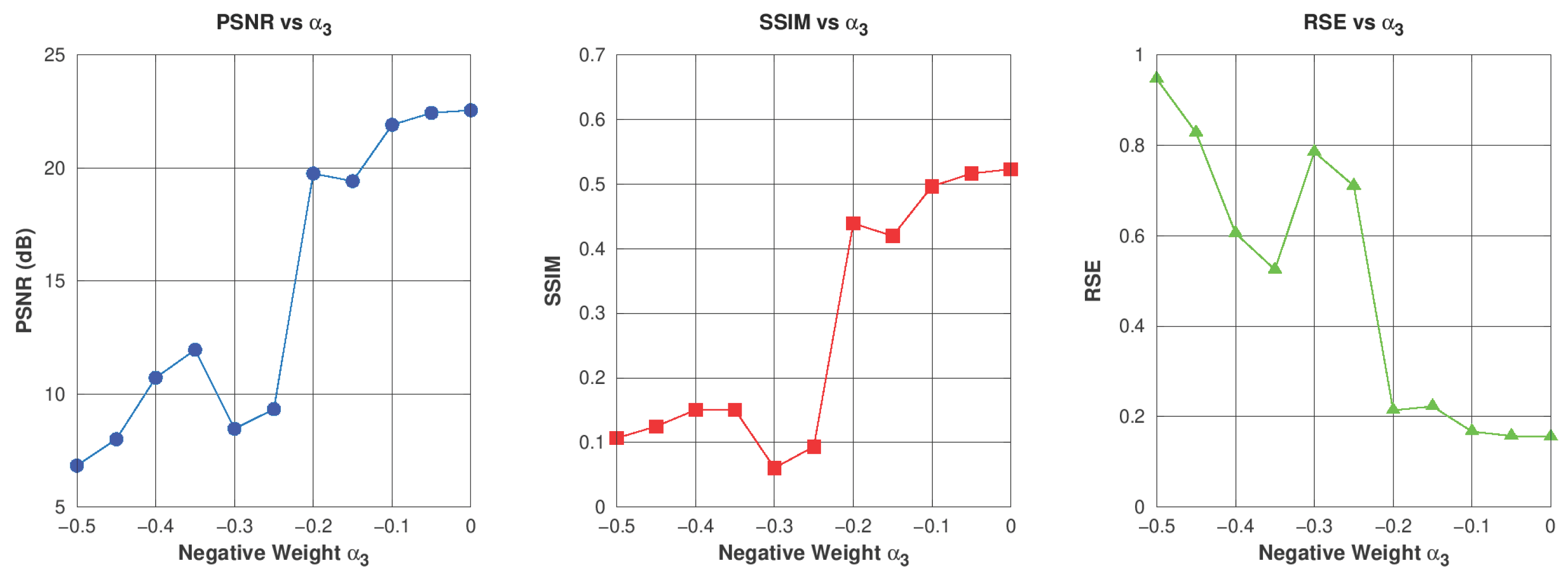
The weight parameters $\mathit{\alpha }=[{\alpha }_1,{\alpha }_2,{\alpha }_3]$ balance the contributions of different tensor modes in FlexHaLRTC. To investigate the impact of the negative weight parameter ${\alpha }_3$, we conducted sensitivity experiments on the Baboon image at a 90% missing rate, varying ${\alpha }_3$ from $-0.5$ to 0 while maintaining ${\alpha }_1={\alpha }_2=(1-{\alpha }_3)/2$.

As shown in Figure 3, moderate negative weights in the color mode (${\alpha }_3\in [-0.3,-0.05]$) consistently outperform purely positive configurations, with a clear PSNR improvement peak. However, extreme negative weights (${\alpha }_3<-0.4$) lead to a sharp degradation in performance and potential numerical instability. This empirical observation supports our choice of ${\alpha }_3=-0.1$ as a robust default for natural image completion.

4.2.4. Sensitivity Analysis of Penalty Parameter $\rho$

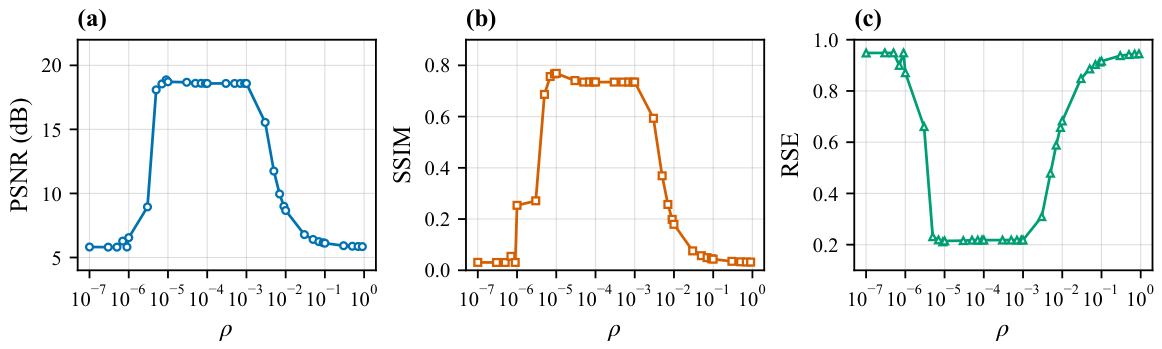
The penalty parameter $\rho$ in the ADMM framework plays a critical role in balancing the convergence speed and solution accuracy. To systematically analyze the impact of $\rho$, we conducted sensitivity experiments on the Baboon image at a 90% missing rate, testing 35 different $\rho$ values spanning seven orders of magnitude from $1\times {10}^{-7}$ to $1\times {10}^{-1}$.

Figure 4 illustrates the performance variation with respect to the penalty parameter $\rho$. The results suggest an effective plateau region roughly between $5\times {10}^{-6}$ and $1\times {10}^{-3}$, where the model maintains good reconstruction accuracy and limited sensitivity to parameter variations. Outside this region, performance degrades due to either insufficient regularization or excessive penalty. Consequently, we set $\rho =1\times {10}^{-5}$ as the default parameter, which lies within this effective range and provides a practical balance between reconstruction quality and numerical stability.

4.2.5. Algorithm Stability Analysis

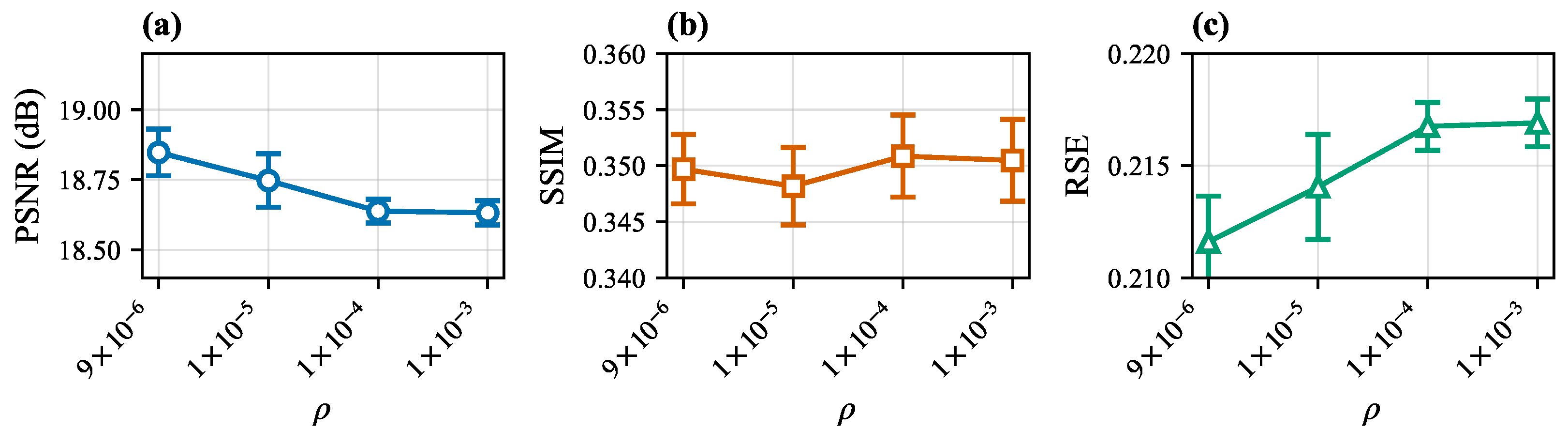
To assess robustness, we repeated the experiment 10 times with different random seeds (42–51) at four representative values of $\rho$ ($9\times {10}^{-6}$, $1\times {10}^{-5}$, $1\times {10}^{-4}$, and $1\times {10}^{-3}$).

Figure 5 shows low run-to-run variance in the effective $\rho$ range (PSNR standard deviation below 0.1 dB; RSE standard deviation below 0.003), suggesting stable empirical behavior under random missing patterns. Since this trend is consistent with the $\rho$-sensitivity results, we treat stability as a supplementary robustness check rather than a separate core finding.

4.2.6. Visual Quality Assessment

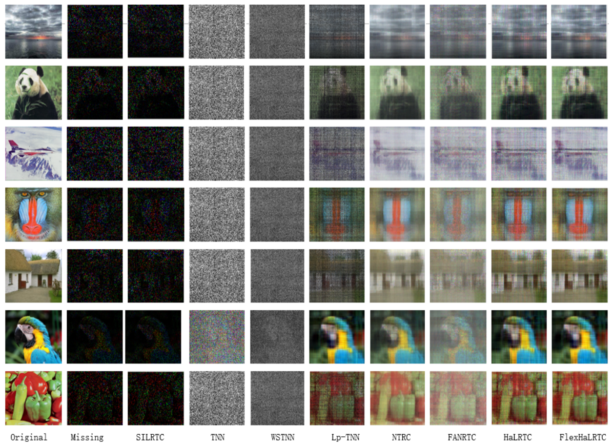
To visually demonstrate the effectiveness of our method, Figure 6 presents a comprehensive comparison of reconstruction results for seven test images at a 90% missing rate.

FlexHaLRTC generally provides competitive visual quality (Figure 6), with improved edge preservation and artifact suppression on several images. For instance, it recovers the structural details of House and the textures of Baboon more clearly than SILRTC and TNN. However, the latest results also show that HaLRTC performs better on some highly smooth or strongly correlated cases (such as Cloudy), while Pepper remains an exception, where HaLRTC is clearly better. To support this observation, we computed RGB inter-channel correlations on the seven test images: the mean pairwise correlation of Pepper is 0.5315 (R-G: 0.2944, R-B: 0.4341, G-B: 0.8661), lower than highly correlated images, such as Cloudy (0.9699), House (0.9567), and Panda (0.9678). This weaker cross-channel coupling may partly explain the reduced benefit of a negative color-mode weight on Pepper. Overall, the visual ranking is broadly consistent with the quantitative results.

4.2.7. Quantitative Performance Analysis

Table 1. Quantitative comparison of image completion methods at a 90% missing rate. Blue indicates best performance.

Missing Rate = 90%		Method
Image	Evaluation	SILRTC	WSTNN	Lp-TNN	TNN	NTRC	FANTRC	HaLRTC	FlexHaLRTC
Cloudy	RSE	0.997	0.495	0.494	0.783	0.153	0.400	0.103	0.118
	PSNR	5.43	11.51	11.49	7.48	22.27	15.46	25.17	23.96
	SSIM	0.0161	0.0430	0.1427	0.0074	0.5924	0.3136	0.6654	0.6057
	time	7.9	42.6	4.5	4.2	55.1	26.9	62.0	62.7
Panda	RSE	0.999	0.569	0.552	0.929	0.237	0.570	0.196	0.190
	PSNR	6.32	11.29	11.48	6.60	19.71	13.89	20.48	20.72
	SSIM	0.0189	0.0428	0.1396	0.0093	0.4724	0.2169	0.4690	0.4397
	time	8.0	21.2	4.3	2.5	56.1	27.8	64.4	65.0
Airplane	RSE	0.999	0.513	0.544	0.620	0.175	0.341	0.141	0.139
	PSNR	2.69	7.70	8.01	6.04	18.37	13.61	19.68	19.84
	SSIM	0.0109	0.0383	0.0690	0.0124	0.4526	0.1654	0.4807	0.4790
	time	8.3	21.2	4.3	1.9	54.3	26.1	62.8	64.1
Baboon	RSE	0.998	0.508	0.547	0.799	0.267	0.517	0.236	0.215
	PSNR	5.36	11.23	10.34	7.31	17.80	13.31	17.89	18.72
	SSIM	0.0287	0.0572	0.1107	0.101	0.3487	0.1843	0.3362	0.3480
	time	8.3	21.2	4.3	2.2	59.1	27.7	62.4	65.9
House	RSE	0.998	0.488	0.541	0.734	0.221	0.489	0.169	0.158
	PSNR	5.13	10.90	11.26	7.31	19.43	13.95	20.92	21.49
	SSIM	0.0576	0.0458	0.0101	0.0186	0.5048	0.2684	0.5365	0.5239
	time	8.0	21.1	4.4	2.2	60.2	29.4	64.4	65.7
Parrot	RSE	0.898	0.730	0.661	1.163	0.386	0.882	0.306	0.295
	PSNR	8.11	10.39	11.14	6.34	17.66	12.60	17.94	18.26
	SSIM	0.0699	0.0331	0.3985	0.0096	0.4756	0.1985	0.4744	0.4340
	time	7.8	20.9	4.4	0.7	56.7	27.3	65.7	63.7
Pepper	RSE	0.998	0.598	0.586	0.917	0.339	0.588	0.283	0.339
	PSNR	6.06	10.62	9.91	6.81	16.74	13.15	17.00	15.45
	SSIM	0.0889	0.0401	0.1147	0.0102	0.4009	0.1552	0.3442	0.2639
	time	7.8	20.7	4.3	2.6	57.5	26.8	65.9	64.2

reports the quantitative evaluation at a 90% missing rate. The results demonstrate that FlexHaLRTC achieves superior performance on the majority of the test set, attaining the highest PSNR or lowest RSE on five out of seven images. Compared to the baseline HaLRTC, FlexHaLRTC provides consistent improvements across most natural scenes, such as House (21.49 dB vs. 20.92 dB) and Baboon (18.72 dB vs. 17.89 dB).

While the average PSNR across all seven images shows a marginal decrease of 0.09 dB, this is primarily attributed to the significant performance gap observed in two specific cases: Cloudy and Pepper. As discussed in Section 3.3, our weight configuration ${\alpha }_3=-0.1$ leverages inter-channel correlations. In images like Pepper, where the cross-channel coupling is relatively weak (mean correlation 0.5315), the benefit of negative color-mode weighting is diminished. However, the consistent gains on the other five images suggest that the proposed signed-weight strategy effectively enhances the expressive power of the unfolding-based model for general natural images. In terms of efficiency, both FlexHaLRTC and HaLRTC exhibit comparable computational costs, typically requiring 62–66 s per image.

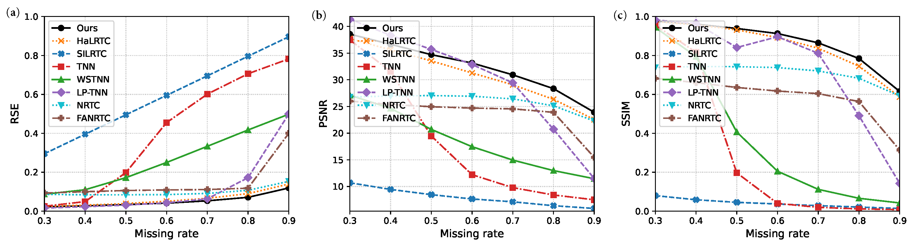
Figure 7 illustrates performance trends from a 30% to 90% missing rate on the Cloudy image. The three panels report RSE, PSNR, and SSIM, respectively. FlexHaLRTC performs competitively across the full range and shows more noticeable advantages at higher missing rates. In particular, the gap to HaLRTC becomes more visible beyond 70%, suggesting that the linear-combination weighting is especially useful in high-sparsity settings.

4.3. Cross-Dataset Generalization on Hyperspectral Imaging

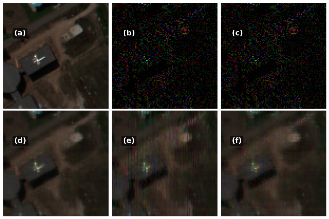
To demonstrate the cross-dataset generalization capability of the proposed algorithm, we evaluated its performance on the standard Pavia University hyperspectral image (HSI) dataset. The original data were cropped to a $100\times 100\times 103$ sub-volume to serve as a 3-way tensor. We simulated a severe missing scenario with an 80% random missing rate.

Using the weight configuration $\mathit{\alpha }=[0.6,0.5,-0.1]$, FlexHaLRTC successfully reconstructed the hyperspectral data, achieving a PSNR of 28.01 dB, an SSIM of 0.7674, and an RSE of 0.180. These results were compared with several baseline methods: SiLRTC (PSNR: 14.10 dB), HaLRTC (PSNR: 31.21 dB), and Matrix Completion (MC) (PSNR: 27.01 dB). These quantitative results confirm that the proposed linear combination model and its corresponding optimization framework maintain stable execution and robust recovery performance across diverse data modalities, extending beyond standard RGB natural images. The visual comparison is shown in Figure 8.

4.4. Color Image Restoration Under Structured Block Missing

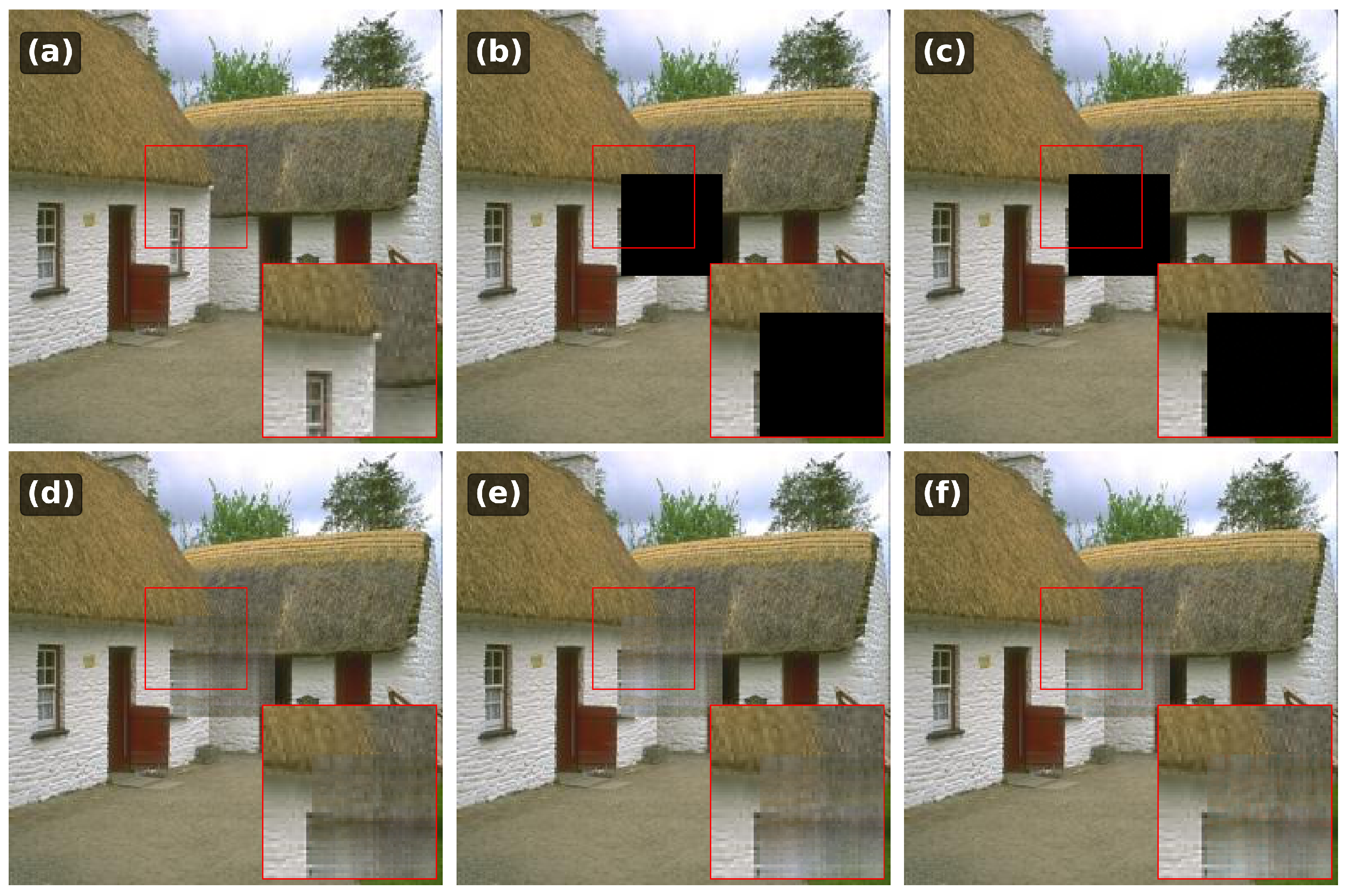
In practical applications, missing data often appears in contiguous structured blocks rather than random isolated pixels. To evaluate the robustness of FlexHaLRTC against such challenging scenarios, we conducted a structured block missing experiment on the standard House image ($256\times 256$). A contiguous $60\times 60$ block of data was removed from the center of the image, severely disrupting the continuous structural information of the scene.

FlexHaLRTC was comprehensively compared against standard algorithms, including HaLRTC and SiLRTC, with Matrix Completion (MC) being applied on the unfolded matrix. The quantitative results demonstrate the significant advantage of the proposed method: FlexHaLRTC achieved a PSNR of 29.47 dB, SSIM of 0.9623, and RSE of 0.063. It outperformed not only HaLRTC (PSNR: 28.17 dB) and SiLRTC (PSNR: 18.32 dB) by a large margin, but also marginally surpassed the Matrix Completion (MC) baseline (PSNR: 29.35 dB). Visually, FlexHaLRTC better preserves the geometric continuity of the occluded regions, confirming that the flexible weight adjustment provides critical regularizations for structured missing data recovery. The visual results with zoom-in details are presented in Figure 9.

5. Video Completion Experiments

5.1. Video Dataset and Experimental Configuration

To further assess the capabilities of FlexHaLRTC in temporal data completion, we evaluate its performance on video completion tasks using the standard Akiyo and Cricket video sequences, widely used benchmarks in video processing research. The original video sequences consist of frames at a CIF resolution ($352\times 288$ pixels). For computational efficiency and a fair comparison with baseline methods, we resized all frames to $176\times 144$ pixels using bicubic interpolation while preserving the aspect ratio. We selected frames 1–100 for our experiments to ensure sufficient temporal correlation while maintaining reasonable computational cost.

5.1.1. Video-Specific Implementation Details

For video completion experiments, we employed two distinct tensor formulations. The first approach is single-frame completion, where each frame is treated independently as a 3D tensor with dimensions of height, width, and color channels. The second approach is multi-frame completion, where consecutive frames are stacked into a 4D tensor with dimensions of height, width, color channels, and time. The 4D formulation enables exploitation of temporal correlations across frames, leading to improved temporal consistency.

We simulated random pixel loss at four distinct missing rates of 20%, 40%, 60%, and 80%. For each missing rate, we generated 5 different random missing patterns and reported average performance metrics. The missing patterns were generated using uniform random sampling without replacement, consistent with the image completion experiments.

5.1.2. Algorithm Configuration for Video Completion

For video experiments, we compared FlexHaLRTC against three representative baselines (NTRC, FANTRC, and HaLRTC). We limited the baseline set to methods that are directly applicable to video tensors under our computational budget and implementation setting—to keep the comparison protocol consistent and tractable. To maintain consistency with the image experiments, we followed the same parameter-selection rationale rather than tuning separate settings for each missing rate or test case. Specifically, the penalty parameter and iteration budget were kept unchanged ($\rho ={10}^{-5}$ and $K=150$ for both FlexHaLRTC and HaLRTC). For FlexHaLRTC, the single-frame setting directly adopts the 3D image configuration $\mathit{\alpha }=[0.6,0.5,-0.1]$. In the multi-frame setting, this design principle is extended to the temporal mode: positive weights are assigned to the two spatial modes and the temporal mode, while a mild negative weight is retained on the color mode to avoid over-regularizing inter-channel correlations, leading to $\mathit{\alpha }=[0.5,0.5,-0.3,0.3]$.

HaLRTC: Uniform weights ($\mathit{\alpha }=[0.25,0.25,0.25,0.25]$ for 4D, and $[1/3,1/3,1/3]$ for 3D), penalty parameter $\rho ={10}^{-5}$, and fixed maximum iterations $K=150$.

NTRC: Tensor ring rank $(r_1,r_2,r_3,r_4)=(8,8,8,8)$ for 4D tensors, learning rate $\eta =0.01$, maximum iterations $K=300$, convergence tolerance $ϵ={10}^{-5}$.

FANTRC: Adaptive tensor ring rank with maximum rank 12, learning rate $\eta =0.01$, maximum iterations $K=300$, convergence tolerance $ϵ={10}^{-5}$.

5.2. Single-Frame Completion Results

In the single-frame scenario, each video frame is treated independently as a 3D tensor with the following dimensions: height × width × color channels. This formulation allows for a direct application of the image completion methodology to video data. While this approach does not exploit temporal correlations between frames, it provides a useful reference setting and remains computationally simple.

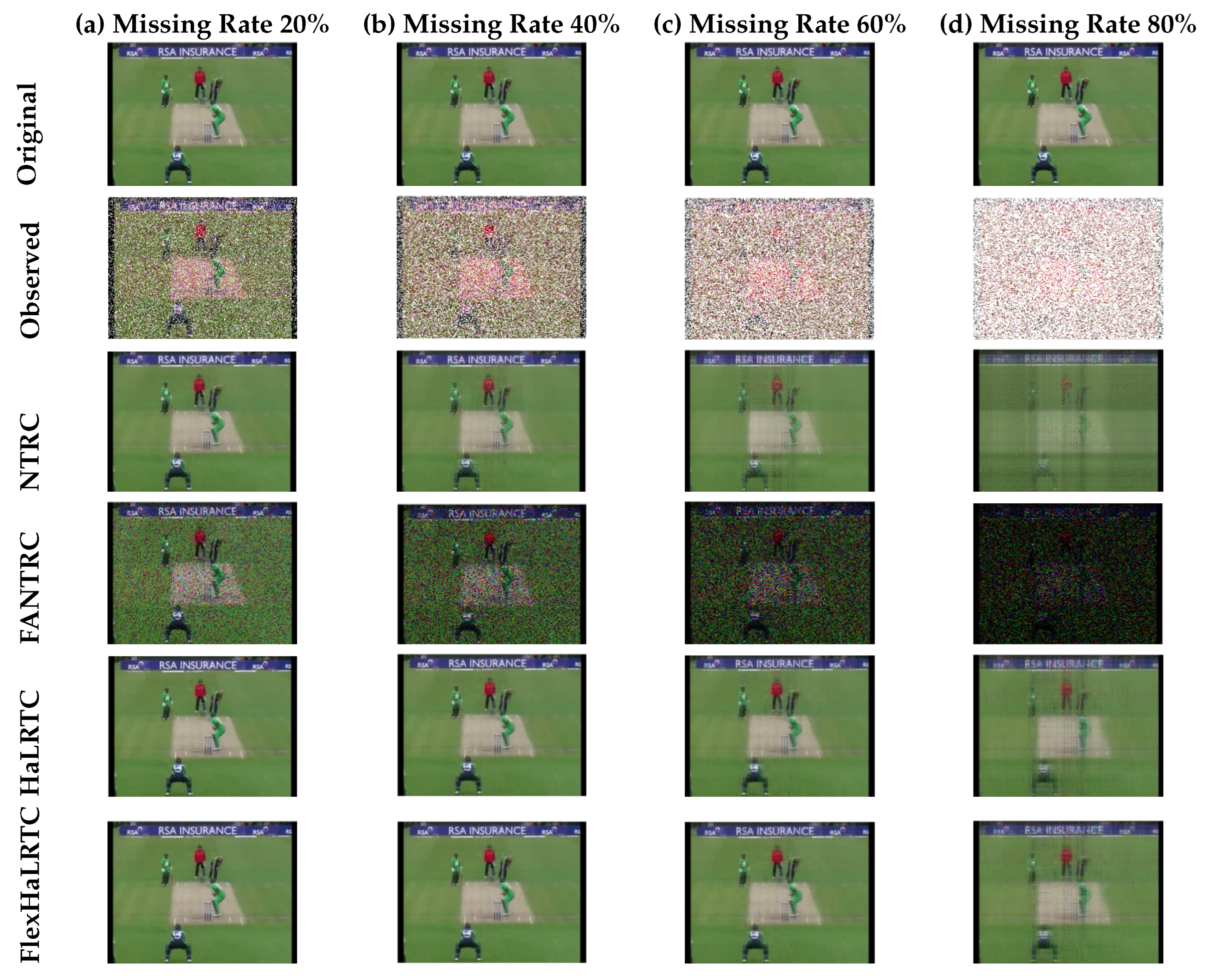
Figure 10 presents a visual comparison of reconstruction results across four missing rates (20%, 40%, 60%, and 80%) for a representative frame from the Akiyo sequence.

As shown in Figure 10, visual differences become more pronounced as the missing rate increases. At a 20% missing rate, most methods produce acceptable results, while FlexHaLRTC and HaLRTC preserve finer details. At 40% and 60%, NTRC shows increasing blur and FANTRC degrades more noticeably; FlexHaLRTC remains visually competitive with clearer facial structures. At 80%, FlexHaLRTC and HaLRTC still recover recognizable facial content, with FlexHaLRTC showing fewer visible artifacts in this example.

Table 2. Quantitative comparison of single-frame video completion. Blue indicates best; bold indicates second best.

Missing Rate	Metric	NTRC	FANTRC	HaLRTC	FlexHaLRTC
20%	PSNR (dB)	33.21	14.51	39.52	40.38
	SSIM	0.942	0.178	0.983	0.980
	RSE	0.0027	0.2002	0.0006	0.0005
40%	PSNR (dB)	28.67	11.50	33.66	35.60
	SSIM	0.870	0.118	0.949	0.957
	RSE	0.0077	0.4000	0.0024	0.0016
60%	PSNR (dB)	25.60	9.75	29.09	30.73
	SSIM	0.802	0.081	0.881	0.904
	RSE	0.0155	0.5991	0.0070	0.0048
80%	PSNR (dB)	21.32	8.49	24.37	25.38
	SSIM	0.627	0.052	0.743	0.771
	RSE	0.0417	0.7996	0.0207	0.0164

provides the quantitative evaluation and broadly agrees with the visual comparison.

FlexHaLRTC achieves the highest PSNR and lowest RSE in this table across all missing rates. For example, at a 40% missing rate, it improves over HaLRTC by 1.94 dB. At a 80% missing rate, it attains 25.38 dB PSNR and 0.771 SSIM, indicating that the reconstruction quality remains reasonable under severe sparsity.

While single-frame completion treats each frame independently, video data exhibits strong temporal correlations that can be exploited for improved reconstruction quality. In multi-frame completion, we stack consecutive frames into a 4D tensor with the following dimensions: height × width × color × time. This formulation allows the algorithm to leverage temporal redundancy, where similar content appears across adjacent frames.

The key challenge in multi-frame video completion is maintaining temporal consistency—ensuring smooth transitions between reconstructed frames without flickering artifacts. Traditional frame-independent methods often produce temporarily inconsistent results, where reconstruction quality varies significantly from frame to frame.

Table 3. Quantitative performance of FlexHaLRTC for multi-frame video completion at a 50% missing rate.

Sequence	Missing Rate	Avg. PSNR (dB)	Avg. SSIM	Avg. RSE
Akiyo	50%	30.12	0.9116	0.0048
Cricket	50%	30.31	0.9056	0.0053

summarizes the quantitative performance of FlexHaLRTC across two representative video sequences with different motion characteristics. The Akiyo sequence contains a relatively static background and slow head motion, while the Cricket sequence involves rapid athletic movements.

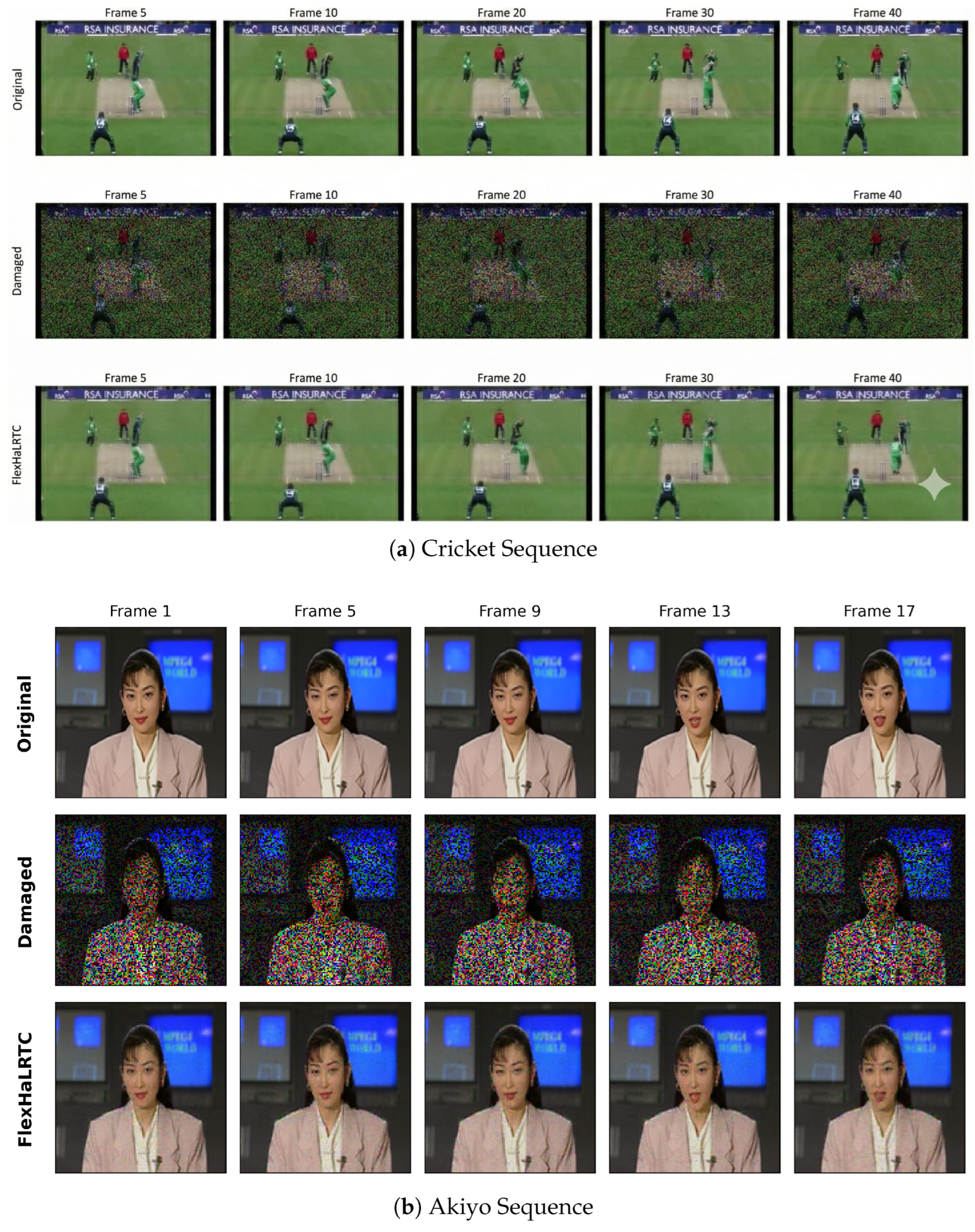
Figure 11 shows consecutive frames from the Cricket (a) and Akiyo (b) sequences at a 50% missing rate. The reconstructed sequences appear temporally smooth and visually consistent. For the Akiyo sequence, FlexHaLRTC achieves an average PSNR of 30.12 dB and SSIM of 0.9116, as shown in Table 3, demonstrating its high restoration quality even at high missing rates.

Across 100 frames of the Akiyo sequence, the average PSNR/SSIM values are 28.45 dB/0.876 versus 26.08 dB/0.831 for frame-independent processing. These results suggest that the linear-combination framework can be extended to 4D tensors and that it effectively improves temporal consistency in this setting.

6. Conclusions

This paper introduced FlexHaLRTC, a tensor completion method that replaces the standard convex combination of nuclear norms with a linear combination, allowing for negative weight parameters to be obtained. We proposed an extended singular value thresholding (SVT)-style update to handle both shrinkage (for positive weights) and expansion (for negative weights) of singular values within an ADMM-based algorithm.

Experiments on color image inpainting and video completion indicate that FlexHaLRTC performs competitively against the compared baselines, with more noticeable gains in several high-missing-rate settings. Negative weights appear to be useful for modeling mode interactions in many cases, yielding improvements in PSNR, SSIM, and RSE on most tested images. In addition, the video experiments follow the same parameter-selection rationale as the image experiments, suggesting that the proposed signed-weight strategy may transfer beyond a single data modality. However, the current weight selection relies on a grid search, and its generalization across broader data types still requires further study.

Future research directions include (1) developing adaptive or data-driven methods for automatic weight selection, (2) extending the linear combination framework to other tensor decomposition models such as tensor train and Tucker decomposition, and (3) providing a more rigorous theoretical analysis of the optimization dynamics induced by signed weights.