ARQ2: Toward Stability-Aware Hybrid Optimization on Complex and Noisy Search Problems

Abstract

ARQ2 is introduced as a next-generation extension of the ARQ (Archive-guided Roulette-based with Quarantine) optimization framework, which was originally established as a cohesive strategy for achieving stable performance on difficult and noisy search landscapes. While rooted in the core principles of the original design, ARQ2 advances this foundation through a more refined integration of adaptive search, archive-guided exploration, controlled replacement, and robustness-aware population management. In doing so, it moves beyond the level of a simple algorithmic modification and emerges as a distinct methodological development within hybrid continuous optimization. Its significance lies in shaping a more mature and experimentally substantiated variant that promotes dependable behavior, consistent search quality, and balanced exploration–exploitation dynamics across diverse optimization environments. Empirical evaluation against nine established optimizers on 36 continuous optimization problems yields an overall average rank of 1.958, with 25 rank-1 placements and a mean-value improvement over ARQ on 21 out of 36 problems, confirming the stronger robustness and repeated-run reliability of the proposed design. As such, ARQ2 contributes to the ongoing development of stability-oriented optimization methodologies and reinforces the scientific relevance of this design line in the contemporary literature.

1. Introduction

This study considers continuous black-box minimization over a bounded hyper-rectangular domain, where only pointwise evaluations of the objective function are assumed to be available and derivative information may be unavailable. In constrained settings, the search is restricted to the feasible subset of the bounded domain, while bound violations may be repaired through projection and more general constraint violations may be absorbed through penalty-based formulations. This viewpoint is standard in derivative-free and constrained optimization, especially when the objective function is nonlinear, multimodal, noisy, or computationally expensive [1,2].

$$\underset{\mathbf{x}\in \Omega }{\min }f\left(\mathbf{x}\right),\Omega ={\displaystyle \prod _{j=1}^n}[l_j,u_j]\subset {\mathbb{R}}^n$$

(1)

Given an evaluation budget N, an optimizer produces candidate points ${\mathbf{x}}^{\left(1\right)},{\mathbf{x}}^{\left(2\right)},\dots ,{\mathbf{x}}^{\left(N\right)}$ and tracks the best-so-far objective value defined by

$$f^{★}\left(m\right)=\underset{1\le \tau \le m}{\min }f\left({\mathbf{x}}^{\left(\tau \right)}\right)$$

(2)

Over R independent runs, terminal performance is summarized by

$$\mathrm{Best}=\underset{1\le r\le R}{\min }{f}_r^{★}\left(N\right),\mathrm{Mean}={\displaystyle \frac{1}{R}}{\displaystyle \sum _{r=1}^R}{f}_r^{★}\left(N\right)$$

(3)

This compact formulation is sufficient for benchmarking derivative-free optimizers under a fixed computational budget and for comparing their terminal effectiveness across repeated runs [1].

The modern optimization literature contains a wide spectrum of algorithmic paradigms developed for hard nonlinear and black-box search problems. Representative examples include simulated annealing [3], particle swarm optimization [4], covariance matrix adaptation evolution strategy [5], ant system [6], tabu search [7], scatter search [8], harmony search [9], artificial bee colony [10], firefly algorithm [11], cuckoo search [12], bat algorithm [13], teaching–learning-based optimization [14], gravitational search algorithm [15], grey wolf optimizer [16], whale optimization algorithm [17], biogeography-based optimization [18], invasive weed optimization [19], shuffled frog-leaping algorithm [20], memetic algorithms [21], and estimation of distribution algorithms [22].

This methodological diversity highlights a central feature of continuous optimization: no single search mechanism is uniformly reliable across all problem classes, and practical performance depends strongly on how exploration, exploitation, adaptation, and population diversity are coordinated. As a result, contemporary research has increasingly emphasized robust search behavior, parameter control, and strategy adaptation rather than purely static algorithmic designs [1,21,22].

Within this broad landscape, Differential Evolution (DE) has become one of the most influential frameworks for real-parameter optimization [23,24,25]. Its compact algorithmic structure can induce markedly different search behaviors through the choice of mutation base vector, difference scheme, and crossover operator. Classical strategies range from the exploratory DE/rand/1/bin, which uses a randomly selected base vector and promotes diversity, to the exploitative DE/best/1/bin, which perturbs the incumbent solution and accelerates local convergence at the risk of premature convergence [23,24,25]. Intermediate schemes such as DE/current-to-best/1/bin balance these tendencies by simultaneously attracting each individual toward the best solution and injecting a differential perturbation term [23,25]. The most influential modern realization of this principle is DE/current-to-pbest/1/bin, popularized by JADE [26], which replaces the unique best individual with a solution drawn from the top p% of the population and extends the difference vector to include an external archive, thereby combining directed elite guidance with historical diversity. The suffix/bin denotes binomial crossover, where each coordinate is updated independently, in contrast to/exp crossover, which updates a contiguous block [23,25]. The same strategic sensitivity applies to the control parameters F and CR, motivating a large body of work on self-adaptation, strategy adaptation, archive usage, and success-history-based parameter control, with representative milestones such as JADE, CoDE [27], SHADE [28], and L-SHADE [29]. Taken together, these developments established that the effectiveness of DE depends on the coordinated interaction of mutation strategy, crossover policy, parameter memories, archive usage, and population management, providing the conceptual basis from which modern hybrid, adaptive, and stability-oriented optimizers are constructed [24,25,26,27,28,29].

The empirical study further situates the proposed ARQ2 against a heterogeneous set of established and recent optimizers, namely its predecessor ARQ [30], the cooperative ensemble EA4Eig [31,32], the competition-oriented jSO [33], the classical self-adaptive DE variant jDE [34], the recent multi-operator mLSHADE-RL [35], the swarm-based CLPSO [36], the hybrid DE framework TRIDENT-DE [37], the constrained-optimization-oriented UDE-III [38] etc. This selection was designed to cover multiple search philosophies, including success-history adaptation, self-adaptation, strategy adaptation, cooperative and ensemble search, archive-assisted differential evolution, swarm intelligence, and hybrid restart mechanisms, thereby avoiding a comparison restricted to a single algorithmic family.

Several of these competitors are also closely connected to the IEEE Congress on Evolutionary Computation (CEC) ecosystem. jSO [33] was introduced in the context of the CEC 2017 single-objective real-parameter optimization track, EA4Eig [31,32] originates from the cooperative model proposed for the CEC 2022 single-objective numerical optimization setting and was later analyzed as the winner of that competition, mLSHADE-RL [35] was proposed for the CEC 2024 single-objective bound-constrained competition while explicitly extending LSHADE-cnEpSin, one of the winning lines from CEC 2017, and UDE-III [38] was developed for the CEC 2024 constrained real-parameter competition while building on IUDE/UDE-II, which achieved first rank in the CEC 2018 constrained-optimization competition. By contrast, jDE [34], SaDE [39], and CLPSO [36] serve as canonical literature baselines, whereas ARQ [30] and TRIDENT-DE [37] represent recent methodological baselines from the broader optimization literature rather than direct competition submissions.

This competition-aware choice of baselines is further consistent with the benchmark culture documented by the Al-Roomi repository [40], which curates IEEE CEC databases and disseminates collections including the CEC 2011 real-world optimization suite as well as later real-parameter and constrained benchmark tracks. Consequently, the present study is positioned not only against widely cited standalone optimizers, but also against methods shaped by the evaluation practices of modern CEC benchmark campaigns.

Overall, the preceding discussion highlights that modern continuous optimization is shaped not only by the quality of individual search operators, but also by the way mutation strategies, parameter adaptation, archive usage, population management, and robustness mechanisms are combined into a coherent search design. Although the literature offers a rich set of competitive optimizers, including several methods associated with CEC benchmark campaigns, their behavior remains problem-dependent and no single scheme can be assumed to provide uniformly stable performance across heterogeneous search landscapes. This observation motivates the development of new optimization designs that place greater emphasis on consistency, controlled search dynamics, and robustness under demanding conditions. Against this background, it is worth clarifying how ARQ2 specifically addresses noisy and multimodal search landscapes. With respect to noisy environments, three complementary mechanisms reduce the distorting influence of stochastic fitness perturbations: the quarantine stage suppresses noise-inflated solutions by relocating outliers around the centroid of the better half of the population, the restricted tournament replacement prevents fortuitous noise-driven improvements from displacing well-positioned individuals, and the success-history adaptation accumulates evidence from genuinely successful trials across multiple iterations, making parameter estimates less susceptible to isolated noisy outcomes. With respect to multimodal landscapes, the IDE branch contributes a structurally distinct search dynamic that reduces concentration around a single attractor, the roulette-based scheduler dynamically reallocates resources between branches based on observed credit histories, and the progress-dependent attraction coefficient $K\left(\pi \right)$ provides a principled transition from broader exploration in early stages to focused refinement in later stages, a property that is particularly beneficial in landscapes with multiple competing local optima.

Against this background, the principal contributions of the present study can be summarized as follows. First, ARQ2 introduces an asymmetric hybrid architecture in which two internal search branches, ARQ and IDE, operate on a shared population and a shared external archive, while the quarantine and micro-restart stabilization mechanisms remain attached exclusively to the ARQ side, preserving the corrective role of the original design without duplicating its machinery in the auxiliary branch. Second, an endogenous roulette-based branch scheduler is proposed, which dynamically reallocates computational resources between branches based on observed credit histories and prevents permanent dominance through a principled credit-reset mechanism. Third, a bootstrap phase is introduced to stabilize early credit statistics before competitive branch selection begins. Fourth, the ARQ-side mutation rule is enriched by a progress-dependent attraction coefficient $K\left(\pi \right)$ that modulates elite guidance as a function of the optimization progress ratio, making the inherited search dynamic more flexible within the hybrid environment. Collectively, these contributions define ARQ2 as an integrated hybrid architecture rather than a straightforward combination of existing components.

The remainder of the article is organized as follows. Section 2 presents the design overview of ARQ2 and its relation to ARQ (Section 2.1), followed by the overall workflow and roulette-based scheduling mechanism (Section 2.2). Section 3 describes the experimental configuration and reproducibility protocol (Section 3.1) and the benchmark testbed, covering real-world (Section 3.2.1) and classical non-real-world problems (Section 3.2.2). Section 4 presents the comparative results, including overall rankings and statistical significance analysis, followed by empirical convergence complexity and runtime overhead (Section 4.1), parameter sensitivity analysis (Section 4.2), and strengths and weaknesses of the proposed method (Section 4.3). Section 5 summarizes the principal findings and concluding remarks.

2. ARQ2: A Roulette-Guided Hybrid Extension of ARQ

2.1. Design Overview and Relation to ARQ

ARQ2 is introduced as a hybrid extension of the previously published ARQ framework rather than as a minor operator-level modification. The original ARQ was designed as a cohesive optimization scheme that combines archive-assisted pbest differential evolution, success-history parameter adaptation, restricted tournament replacement, and an event-driven stabilization mechanism based on quarantine and targeted micro-restarts. Since these core components have already been presented in detail in the original ARQ study, they are not repeated here exhaustively. Instead, the present section focuses on the architectural modifications through which ARQ2 extends that design line [30].

The central idea behind ARQ2 is to preserve the stability-oriented backbone of ARQ while embedding a second internal search branch derived from IDE within the same optimization process. In contrast to ARQ, which evolves the population through a single cohesive update cycle, ARQ2 operates through a controller-driven hybrid structure in which two internal heuristics, namely an ARQ branch and an IDE branch, act on a shared population and a shared external archive. The method explicitly implements this hybrid identity at the design level, as reflected by its own definition as an “ARQ/IDE roulette” scheme with quarantine, ARQ-only micro-restart, and a jSO-style attraction coefficient. This already indicates that the proposed method should be interpreted not as a reformulation of ARQ, but as a broader search architecture built upon it [30,33].

More specifically, ARQ2 retains from ARQ the archive-based search memory, the success-history adaptation of F and CR, the neighborhood-aware RTR replacement logic, and the robustness-oriented maintenance philosophy. However, it augments this inherited core in four important ways. First, it introduces an IDE-based branch with its own search dynamics and per-individual parameter memories. Second, it employs a roulette-guided branch scheduler that dynamically decides which internal heuristic will be activated at each iteration. Third, it includes an early bootstrap phase that temporarily favors the ARQ branch before the branch-selection statistics become informative. Fourth, the ARQ-side trial construction is enriched by a jSO-style coefficient K, which modulates the attraction toward elite exemplars and makes the inherited ARQ mutation rule more flexible inside the hybrid environment. These additions collectively define the methodological identity of ARQ2 [17,30,31,33].

An equally important aspect of the design is that the hybridization remains intentionally asymmetric. Although ARQ2 contains two internal branches, the quarantine mechanism and the targeted micro-restart remain attached only to the ARQ side. This choice is not incidental, rather, it preserves the corrective and regenerative role that distinguished ARQ in the first place, while allowing the IDE branch to contribute behavioral diversity without duplicating the same stabilization machinery. In addition, the two branches are not fully isolated from one another, since they operate on shared population state and archive memory, while ARQ-side events may also trigger IDE-parameter inheritance or reset actions. Consequently, ARQ2 is better characterized as an integrated hybrid architecture than as a simple portfolio of independently running optimizers [30].

From this perspective, the contribution of ARQ2 lies less in the invention of a single new search operator and more in the coordinated redesign of the optimization workflow. The method extends ARQ by combining a stability-aware DE backbone with an auxiliary IDE search regime, an endogenous heuristic-selection controller, and asymmetric maintenance mechanisms that preserve robustness while broadening the search behavior. For this reason, the proposed method is presented in the following subsections primarily through its workflow and architectural interactions, rather than through a full rederivation of the already published ARQ components [30].

2.2. Overall Workflow and Roulette-Based Hybrid Scheduling

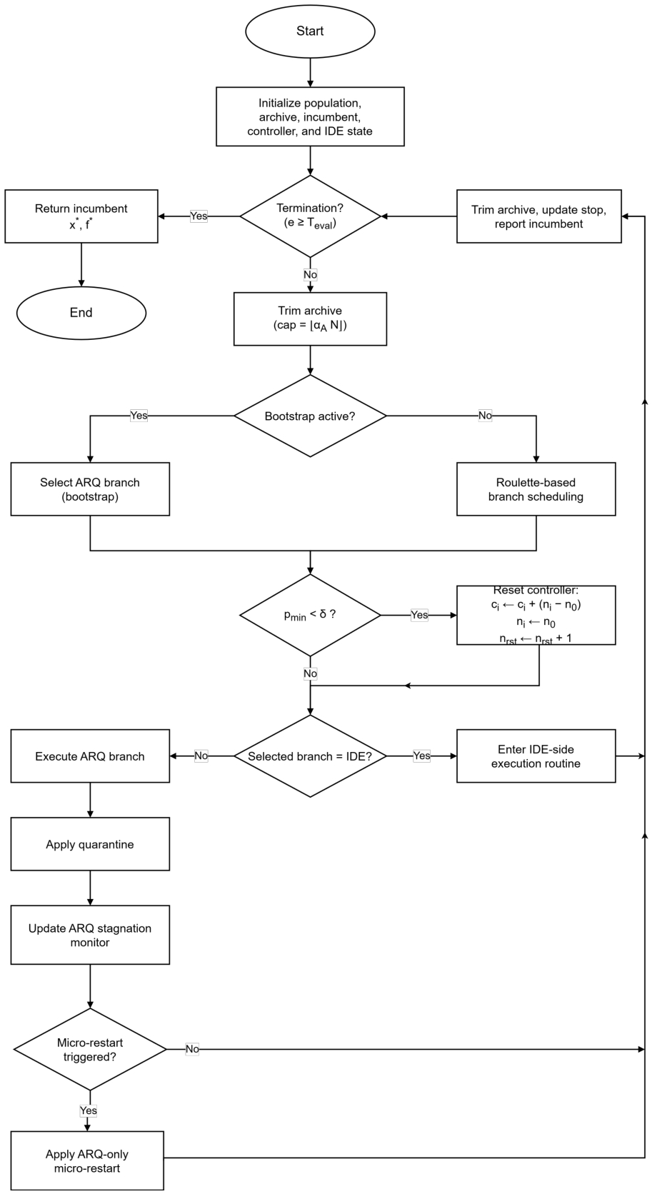
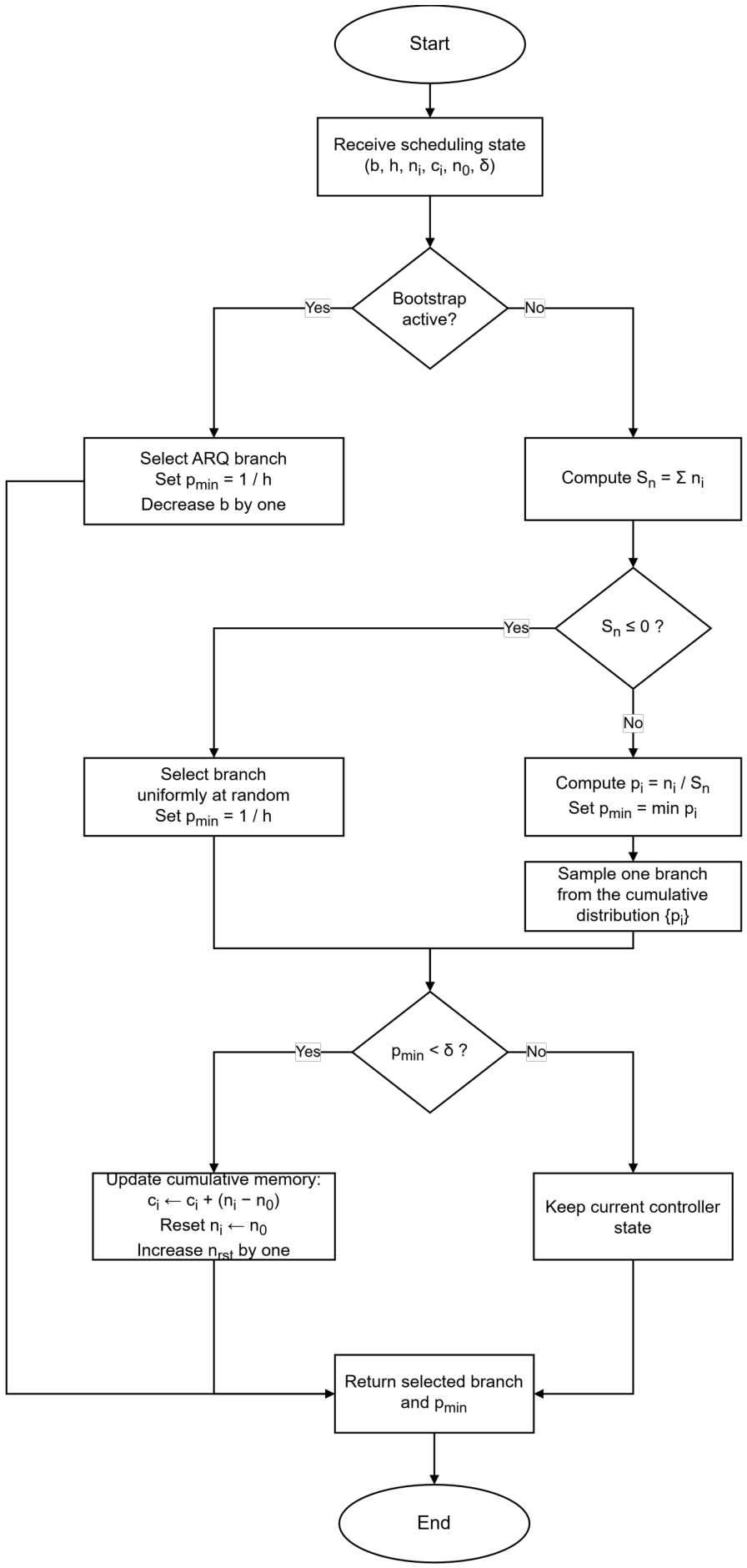
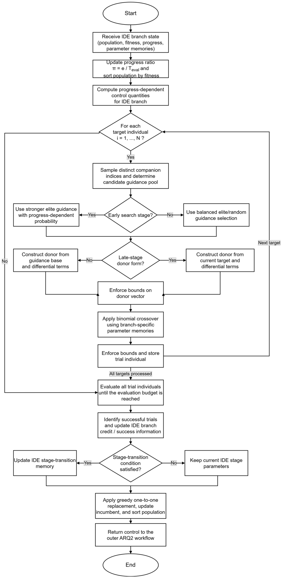
ARQ2 evolves a single population under a hybrid controller that activates one of two internal search branches at each iteration. Let $X={\left\{x_i\right\}}_{i=1}^N$ denote the current population, let A denote the external archive, and let $(x^{*},f^{*})$ denote the incumbent best solution and its objective value. Instead of relying on a single homogeneous update rule, the method follows a controller-driven workflow in which archive maintenance, branch scheduling, branch execution, branch-dependent stabilization, and stopping checks are performed in a fixed sequence. The overall workflow, the roulette-based scheduler, and the IDE-side routine are therefore presented separately in Figure 1, Figure 2 and Figure 3, and in Algorithms 1, 2 and 3, respectively.

At initialization, the method evaluates the initial population, constructs the archive, and identifies the initial incumbent. It also initializes a stagnation monitor through a reference best value $f^{\mathrm{prev}}$ and a non-improvement counter s. The branch scheduler is configured for $h=2$ competing branches, corresponding to ARQ and IDE. A baseline branch credit $n_0$ is assigned to each branch, the reset threshold is set to $\delta =1/\left(5h\right)$, the initial active credits satisfy $n_i=n_0$ for $i=1,2$, the cumulative credit-memory terms satisfy $c_i=0$, and the reset counter is initialized as $n_{\mathrm{rst}}=0$. In addition, a bootstrap counter b is used to enforce the ARQ branch during the first scheduled iterations. To maintain a common notion of search progress across the two branches, the algorithm uses the evaluation-based progress ratio. The value $\delta =1/\left(5h\right)$ was selected to ensure that a reset is triggered before any branch is reduced to near-zero selection probability, while remaining tolerant enough to allow meaningful credit differentiation between branches. For $h=2$, this yields $\delta =0.1$, meaning a reset occurs when one branch holds less than ten percent of the total selection probability.

$$\pi ={\displaystyle \frac{e}{T_{\mathrm{eval}}}},$$

where e denotes the number of consumed function evaluations and $T_{\mathrm{eval}}$ denotes the total evaluation budget.

Algorithm 1 Main workflow of ARQ2

INPUT - f: objective function - $\Omega$: box-constrained search domain - N: population size - $T_{\mathrm{eval}}$: maximum number of function evaluations - p: elite fraction in the ARQ branch - $\xi$: update fraction in the ARQ branch - ${\mu }_F,{\mu }_{CR}$: ARQ parameter means - ${\alpha }_A$: archive-rate coefficient - ${\alpha }_o,{\rho }_o,{\sigma }_q$: quarantine parameters - ${\rho }_w,{\sigma }_r,\tau$: ARQ micro-restart parameters - $h,n_0,\delta ,b$: scheduler parameters - ${\pi }_t,\lambda$: IDE phase-threshold and patience parameters OUTPUT - $x^{*},f^{*}$ INITIALIZATION - Initialize population $X={\left\{x_i\right\}}_{i=1}^N\subset \Omega$ and evaluate all individuals - Set archive $A\leftarrow ⌀$ - Identify the incumbent best pair $(x^{*},f^{*})$ - Set $f^{\mathrm{prev}}\leftarrow f^{*}$ and $s\leftarrow 0$ - Set $n_i\leftarrow n_0$ and $c_i\leftarrow 0$ for $i=1,\dots ,h$ - Set $n_{\mathrm{rst}}\leftarrow 0$ - Set $e\leftarrow N$ - Initialize the bootstrap counter b, the IDE phase threshold ${\pi }_t$, the patience window $\lambda$, the counter ${\lambda }_c\leftarrow 0$, and the individual IDE memories ${\{F_i^{\mathrm{IDE}},C{R}_i^{\mathrm{IDE}}\}}_{i=1}^N$ ARQ2 main pseudocode 01 While $e<T_{\mathrm{eval}}$ do 02       Trim A to size $\lfloor {\alpha }_{A}N\rfloor$ 03       Obtain the selected branch and the updated scheduler state from Algorithm 2 04       If the IDE branch is selected then 05             Apply the IDE branch update according to Algorithm 3 06       Else 07             Apply the ARQ branch update to X and A 08             Apply quarantine-based correction using ${\alpha }_o,{\rho }_o,{\sigma }_q$ 09             If $f^{*}<f^{\mathrm{prev}}$ then 10                  Set $f^{\mathrm{prev}}\leftarrow f^{*}$ 11                  Set $s\leftarrow 0$ 12             Else 13                  Set $s\leftarrow s+1$ 14             Endif 15             If $s\ge \tau$ then 16                  Apply ARQ-only micro-restart to the $\lfloor {\rho }_{w}N\rfloor$ worst individuals around $x^{*}$ 17                  Set $s\leftarrow 0$ 18             Endif 19       Endif 20       Trim A again to size $\lfloor {\alpha }_{A}N\rfloor$ 21       Update the stopping state and report the current incumbent 22       Set e equal to the current number of function evaluations 23 Endwhile 24 Return $x^{*},f^{*}$

At the beginning of each iteration, the archive is first trimmed so that its capacity does not exceed

$$\lfloor {\alpha }_{A}N\rfloor ,$$

where ${\alpha }_A$ is the archive-size coefficient. The controller then determines which branch will be executed. If $b>0$, the ARQ branch is selected deterministically and the bootstrap counter is decreased by one. This is the only stage in which ARQ has strict priority. After the bootstrap stage has ended, neither ARQ nor IDE has permanent priority; instead, both branches compete under the same credit-based scheduler.

Algorithm 2 Roulette-based branch scheduling and credit reset in ARQ2

INPUT - h: number of internal search branches - $n_0$: baseline branch credit - $\delta$: reset threshold - b: bootstrap counter - ${\left\{n_i\right\}}_{i=1}^h$: active branch-credit vector - ${\left\{c_i\right\}}_{i=1}^h$: cumulative reset-memory vector - $n_{\mathrm{rst}}$: reset counter OUTPUT - Selected branch, minimum branch probability, and updated scheduler state Roulette-based branch scheduling and credit reset 01 If $b>0$ then 02      Select the ARQ branch 03      Set $b\leftarrow b-1$ 04      Set $p_{\min }\leftarrow 1/h$ 05      Return the ARQ branch and the updated scheduler state 06 Endif 07 If ${\sum }_{i=1}^h{n}_i\le 0$ then 08      Set $p_i\leftarrow 1/h$ for $i=1,\dots ,h$ 09 Else 10      Set $p_i\leftarrow {\displaystyle \frac{n_i}{{\sum }_{k=1}^h{n}_k}}$ for $i=1,\dots ,h$ 11 Endif 12 Set $p_{\min }\leftarrow {\min }_{1\le i\le h}{p}_i$ 13 Draw $u\sim U(0,1)$ 14 If $u\le p_1$ then select the ARQ branch; otherwise select the IDE branch 15 If $p_{\min }<\delta$ then 16      For $i=1$ to h do 17          Set $c_i\leftarrow c_i+(n_i-n_0)$ 18          Set $n_i\leftarrow n_0$ 19      Endfor 20      Set $n_{\mathrm{rst}}\leftarrow n_{\mathrm{rst}}+1$ 21 Endif 22 Return the selected branch and the updated scheduler state

If

$${\displaystyle \sum _{i=1}^h}{n}_i\le 0,$$

the selection degenerates to a uniform random choice and the minimum branch probability becomes

$$p_{\min }={\displaystyle \frac{1}{h}}.$$

Otherwise, the controller normalizes the active branch credits according to

$$p_i={\displaystyle \frac{n_i}{{\sum }_{k=1}^h{n}_k}},i=1,\dots ,h,$$

and defines

$$p_{\min }=\underset{1\le i\le h}{\min }{p}_i.$$

A branch is then sampled from the cumulative distribution induced by ${\left\{p_i\right\}}_{i=1}^h$. If $p_{\min }<\delta$, the controller performs a reset according to

$$c_i\leftarrow c_i+(n_i-n_0),n_i\leftarrow n_0,i=1,\dots ,h,$$

and increases $n_{\mathrm{rst}}$ by one. Branch credits are updated in proportion to the number of successful individual replacements, so that more productive branches receive higher selection probability. Premature dominance is prevented by two mechanisms: the bootstrap phase stabilizes early credit statistics, and the reset triggered when $p_{\min }<\delta$ restores both branches to their baseline credit $n0$, ensuring sustained competition throughout the search. From an analytical standpoint, the credit-reset mechanism can be interpreted as a safeguard against degenerate branch probability distributions. Without resetting, a transient performance advantage of one branch early in the search could reduce the competitor to a near-zero selection probability, effectively collapsing the hybrid into a single-branch method and eliminating the behavioral diversity that motivates the hybrid design. The reset restores both branches to a common baseline while transferring accumulated deviation to the cumulative memory $c_i$, thereby preserving historical information without allowing it to permanently suppress branch competition. This design is consistent with the theoretical rationale of exploration preservation in adaptive operator selection frameworks, where maintaining a minimum selection probability for all operators is known to prevent premature specialization. Consequently, future branch probabilities are computed from the reset active-credit vector ${\left\{n_i\right\}}_{i=1}^h$, whereas ${\left\{c_i\right\}}_{i=1}^h$ acts only as an accumulated bookkeeping memory.

If the selected branch is ARQ, the method applies a stability-oriented differential update to a subset of $m=\lceil \xi N\rceil$ individuals, where $\xi \in (0,1]$ is the agent-update fraction. For a target vector $x_i$, a trial donor is generated in the form

$$v_i=x_i+K\left(\pi \right)\left(x_{p\mathrm{best}}-x_i\right)+F_i\left(x_{r_1}-{\tilde{x}}_{r_2}\right),$$

where $x_{p\mathrm{best}}$ is selected from the top $\lceil pN\rceil$ individuals, ${\tilde{x}}_{r_2}$ is drawn either from the current population or from the archive, and $F_i$ is the scaling factor sampled from the ARQ success-history mechanism. In the present ARQ2 realization, the attraction coefficient is piecewise defined as

$$K\left(\pi \right)=\left\{\begin{array}{cc}0.7F_i,\hfill & \pi <0.2,\hfill \\ 0.8F_i,\hfill & 0.2\le \pi <0.4,\hfill \\ 1.2F_i,\hfill & \pi \ge 0.4.\hfill \end{array}\right.$$

The offspring vector is then produced through binomial crossover,

$$u_{ij}=\left\{\begin{array}{cc}{v}_{ij},\hfill & {\mathrm{rand}}_{ij}\le C{R}_i\mathrm{or}j=j_{\mathrm{rand}},\hfill \\ x_{ij},\hfill & \mathrm{otherwise},\hfill \end{array}\right.$$

followed by bound handling and replacement through the ARQ acceptance logic. Thus, the ARQ branch preserves the core current-to-pbest differential structure of the original method while using the modified attraction term $K\left(\pi \right)$ and the common outer scheduler.

If the selected branch is IDE, the method applies a progress-dependent differential update with branch-specific memories for mutation and crossover control. To preserve notation consistency with the rest of the manuscript, the IDE-side behavior is also expressed through the same global progress ratio $\pi$. The branch first defines the progress-sensitive elite-pressure term

$${\epsilon }_{\mathrm{IDE}}\left(\pi \right)=0.1+0.9·{10}^{5(\pi -1)}.$$

This quantity determines the size of the elite-guided pool,

$$H\left(\pi \right)=max\{2,\mathrm{round}\left({\epsilon }_{\mathrm{IDE}}\left(\pi \right)N\right)\}.$$

Algorithm 3 IDE branch update in ARQ2

INPUT - $X={\left\{x_i\right\}}_{i=1}^N$: current population - f: objective function - $\Omega$: feasible search domain - $e,T_{\mathrm{eval}}$: current and maximum numbers of function evaluations - ${\pi }_t$: phase-switch progress threshold - $\lambda ,{\lambda }_c$: patience window and consecutive low-success counter - ${\{F_i^{\mathrm{IDE}},C{R}_i^{\mathrm{IDE}}\}}_{i=1}^N$: individual IDE parameter memories - $n_{\mathrm{IDE}}$: credit of the IDE branch OUTPUT - Updated population, incumbent pair, IDE state, and IDE branch credit IDE branch update in ARQ2 01 Set $\pi \leftarrow e/T_{\mathrm{eval}}$ 02 Sort X in nondecreasing objective value 03 Set $\epsilon \left(\pi \right)\leftarrow 0.1+0.9·{10}^{5(\pi -1)}$ 04 If $\pi <{\pi }_t$ then set $S_{\mathrm{th}}\leftarrow 0$; otherwise set $S_{\mathrm{th}}\leftarrow 0.1$ 05 For each $i=1,\dots ,N$ do 06      Sample distinct indices $o,r_1,r_2,r_3\ne i$ 07      Set $m\left(\pi \right)\leftarrow max\{2,\mathrm{round}(\epsilon \left(\pi \right)N\left)\right\}$ 08      If $\pi \le {\pi }_t$ then 09          With probability $0.9\epsilon \left(\pi \right)$, choose $r_1^{★}$ from the best $m\left(\pi \right)$ individuals; otherwise set $r_1^{★}\leftarrow r_1$ 10      Else 11          With probability $0.5$, choose $r_1^{★}$ from the best $m\left(\pi \right)$ individuals; otherwise set $r_1^{★}\leftarrow r_1$ 12      Endif 13      If $\pi >{\pi }_t$ and a Bernoulli trial with parameter $0.5$ succeeds then 14          Set $v_i\leftarrow x_i+F_i^{\mathrm{IDE}}(x_{r_1^{★}}-x_o)+F_i^{\mathrm{IDE}}(x_{r_2}-x_{r_3})$ 15      Else 16          Set $v_i\leftarrow x_o+F_i^{\mathrm{IDE}}(x_{r_1^{★}}-x_o)+F_i^{\mathrm{IDE}}(x_{r_2}-x_{r_3})$ 17      Endif 18      Repair $v_i$ to $\Omega$ 19      Construct trial vector $y_i$ by binomial crossover between $x_i$ and $v_i$ with rate $C{R}_i^{\mathrm{IDE}}$ 20      Repair $y_i$ to $\Omega$, evaluate $f\left(y_i\right)$, and update e 21 Endfor 22 Define the success set $I_s=\{i:f\left(y_i\right)<f\left(x_i\right)\}$ 23 Set $SR\leftarrow |I_s|/N$ 24 Increase $n_{\mathrm{IDE}}$ in proportion to the number of successful replacements 25 If $\pi <{\pi }_t$ then 26      If $SR\le S_{\mathrm{th}}$ then set ${\lambda }_c\leftarrow {\lambda }_c+1$; otherwise set ${\lambda }_c\leftarrow 0$ 27      If ${\lambda }_c\ge \lambda$ then set ${\pi }_t\leftarrow \pi$ 28 Endif 29 For each $i\in I_s$ do 30      Replace $x_i$ with $y_i$ 31      Update the incumbent pair $(x^{*},f^{*})$ if improved 32 Endfor 33 Return the updated IDE state and population

Accordingly, the donor construction follows a progress-dependent mixed strategy. In its guidance-oriented regime, the branch uses

$$v_i=x_o+F_i(x_{r_1}-x_o)+F_i(x_{r_2}-x_{r_3}),$$

where $x_{r_1}$ is selected either from the elite pool of size $H\left(\pi \right)$ or from a standard random index. In the later current-based regime, it may instead use

$$v_i=x_i+F_i(x_{r_1}-x_o)+F_i(x_{r_2}-x_{r_3}).$$

The trial vector is then generated by the same binomial crossover form as above, but with branch-specific crossover memory $C{R}_i$. After evaluation, the IDE branch applies greedy one-to-one replacement. Denoting the offspring by $u_i$, replacement occurs when

$$f\left(u_i\right)\le f\left(x_i\right),$$

or, in the strict variant, when $f\left(u_i\right)<f\left(x_i\right)$. The IDE-side success rate is then

$$SR={\displaystyle \frac{\left|S\right|}{N}},$$

where S is the set of successful offspring. Therefore, within ARQ2, IDE acts as a complete complementary search routine rather than as a single isolated mutation formula.

After branch execution, additional stabilization is applied only when the selected branch is ARQ. The first layer is quarantine-based correction. Let $Q_3$ denote the third quartile of the fitness distribution and let $IQR$ denote the interquartile range. Fitness outliers are identified through

$$\theta =Q_3+{\alpha }_Q·IQR,$$

where ${\alpha }_Q$ is the outlier-sensitivity coefficient. A fraction ${\rho }_Q$ of the detected outliers is then relocated around the center of the better half of the population using Gaussian perturbations scaled by ${\sigma }_Q$. The second layer is an ARQ-only micro-restart activated when

$$s\ge \tau ,$$

where $\tau$ is the stagnation threshold. In that case, the method perturbs the incumbent neighborhood and attempts to replace the worst fraction $\omega$ of the population using Gaussian noise scaled by ${\sigma }_R$.

Finally, the iteration ends with a second archive-trimming stage, followed by the update of the stopping state and the reporting of the current incumbent. Consequently, the execution order of ARQ2 is: archive maintenance, bootstrap-or-roulette scheduling, optional controller reset, execution of the selected branch, ARQ-only stabilization when applicable, and final bookkeeping. This hierarchy also defines the natural order in which the overall flowchart, the roulette-based flowchart, the IDE flowchart, and the three corresponding pseudocodes should appear in the manuscript.

3. Empirical Evaluation Protocol and Benchmark Landscape

3.1. Experimental Configuration and Reproducibility Protocol

All algorithms, including the proposed method and the baseline competitors, were implemented in efficient ANSI C++ and integrated into the open-source OptimSolution framework, which was created by Vasileios Charilogis. The source code is publicly available through the GitHub repository: https://github.com/charilog/optimsolution (accessed: 16 March 2026). Compilation and execution were carried out under Debian 12.12 using GCC 13.4. The experimental platform was a high-performance system equipped with an AMD Ryzen 9 9950X3D processor (16 cores, 32 threads) and 64 GB of DDR4 memory, also running Debian Linux. To capture the stochastic behavior of the methods, each benchmark function was executed in 30 independent runs with different random seeds, while the same fixed objective-function evaluation budget was enforced for all solvers. The budget of 150,000 function evaluations follows the termination criterion established by the CEC 2011 real-world numerical optimization benchmark suite [41], ensuring direct comparability with the related literature. For higher-dimensional problems such as test2n (D = 200), this budget is more restrictive but is retained deliberately so that all methods operate under a uniform computational constraint. The primary reported performance measures were the best and mean objective values obtained at termination, computed over the 30 independent runs for each test problem. In the comparative tables, first-ranked entries are highlighted in green and second-ranked entries in blue, while all parameter settings follow exactly the values reported in

Table 1. ARQ2 parameter settings used in the experiments.

Name	Value	Description
N	100	Population size
$T_{\mathrm{eval}}$	150,000	Maximum number of function evaluations
p	0.12	Top fraction for p-best selection in the ARQ branch
$\xi$	0.60	Agent-update fraction in the ARQ branch
${\mu }_F$	0.60	Initial mean of the scaling factor in the ARQ branch
${\mu }_{CR}$	0.85	Initial mean of the crossover rate in the ARQ branch
$F_{lo}$	0.05	Lower bound imposed on the ARQ scaling factor
$F_{hi}$	1.40	Upper bound imposed on the ARQ scaling factor
${\alpha }_Q$	1.0	Outlier-sensitivity coefficient in the quarantine stage
${\rho }_Q$	0.08	Fraction of detected outliers repaired by quarantine
${\sigma }_Q$	0.10	Gaussian perturbation scale used in quarantine
$\omega$	0.08	Worst-population fraction used in the ARQ micro-restart
${\sigma }_R$	0.18	Gaussian perturbation scale used in the ARQ micro-restart
$\tau$	24	Stagnation threshold for triggering the ARQ micro-restart
${\eta }_{SH}$	0.10	Success-history smoothing coefficient in the ARQ branch
${\alpha }_A$	1.5	Archive-size coefficient
$r_{RTR}$	14	Candidate-pool size used by restricted tournament replacement
h	2	Number of internal branches in the roulette controller
$n_0$	2	Baseline credit assigned to each branch
$\delta$	0.10	Controller reset threshold
b	2	Bootstrap length during which the ARQ branch is enforced
${\pi }_t^{\left(0\right)}$	0.5	Initial phase-switch threshold in the IDE branch
$\lambda$	150	Patience window in the IDE branch

and

Table 2. Parameters of other methods.

Name	Value	Description
N	100	Population size for all methods
JSO
$N{P}_{factor}$	18	Initial population size $N{P}_0=N{P}_{factor}\times Dim$
H	20	Memory size for success-history means $MF$/$MCR$
$pbest$	0.11	Fraction for p-best selection (top-p set).
$archiv{e}_{rate}$	1	Archive size as multiple of NP0 (i.e., archiveMax = archive_rate × NP0).
CLPSO
$c{l}_p$	0.3	Comprehensive learning probability
$cognitiv{e}_{weight}$	1.49445	Cognitive weight
$inerti{a}_{weight}$	0.729	Inertia weight
$mutatio{n}_{rate}$	0.01	Mutation rate
$socia{l}_{weight}$	1.49445	Social weight
EA4Eig
$archiv{e}_{size}$	100	Archive size for JADE-style mutation
$ei{g}_{interval}$	5	Recompute eigenbasis every k iterations
$C{R}_{max}$	1	Upper bound for $CR$
$F_{max}$	1	Upper bound for F
$C{R}_{min}$	0	Lower bound for $CR$
$F_{min}$	0.1	Lower bound for F
$p_{best}$	0.2	pbest fraction (current-to-pbest/1/bin)
$C{R}_{tau}$	0.1	Self-adaptation prob. for $CR$
$F_{tau}$	0.1	Self-adaptation prob. for F
mLSHADE_RL
$archiv{e}_{size}$	500	Archive size
$Memor{y}_{size}$	10	Success-history memory size
$Populatio{n}_{min}$	4	Minimum population size
$p_{bes{t}_{max}}$	0.2	Maximum pbest fraction
$p_{bes{t}_{min}}$	0.05	Minimum pbest fraction
SaDE
$C{R}_{sigma}$	0.1	Std for $CR$ sampling
$F_{gamma}$	0.1	Scale for Cauchy F sampling
$C{R}_{init}$	0.5	Initial $CR$ mean
$F_{init}$	0.7	Initial F mean
$learnin{g}_{period}$	25	Iterations per adaptation window
UDE3
$Populatio{n}_{min}$	4	Minimum population size.
$Memor{y}_{size}$	10	Success-history memory size
$archiv{e}_{size}$	100	Archive size
$p_{bes{t}_{min}}$	0.05	Minimum pbest fraction
$p_{bes{t}_{max}}$	0.2	Maximum pbest fraction.
TRIDENT-DE: See Table 1 here [37]

. Although some competitors such as JSO employ a variable initial population size determined by a problem-dimension-dependent factor, fairness across all compared methods is ensured at the level of the total function evaluation budget rather than at the level of population size. Since all solvers are subject to the same fixed limit of 150,000 function evaluations, differences in population initialization strategy affect only the internal allocation of that budget and do not grant any method an additional computational advantage. To ensure a fair comparison on equal computational terms, local search components embedded in certain competitors were disabled in the present experimental setting. Specifically, the eigenvector-based local refinement of EA4Eig was deactivated, as it introduces an additional layer of exploitation that is absent from the remaining methods and would otherwise render the comparison asymmetric with respect to the per-evaluation computational effort.

3.2. Real-World and Classic Optimization Testbed

Section 3.2 is structured around two complementary benchmark groups in Section 3.2.1 and Section 3.2.2. The first group consists of real-world optimization problems and is included to evaluate the practical utility of ARQ2 under constrained, black-box, simulator-driven, and application-oriented conditions. The second group consists of classical hard benchmark functions and is used to examine core search behavior under controlled settings, including multimodality, ruggedness, ill-conditioning, separability or non-separability, and sensitivity to increasing dimensionality. The joint use of these two benchmark categories reduces the risk of drawing conclusions from a single problem family and supports a more balanced assessment of ARQ2, both in terms of practical applicability and in terms of fundamental robustness across heterogeneous optimization landscapes.

3.2.1. Real World Benchmark Functions

• Uniform Linear Antenna Array Design (half-wavelength spacing, amplitude taper) [antennaarray] [42]
  Objective:
  $AF\left(\theta \right)={\sum }_{n=0}^{N-1}{w}_n{e}^{j\pi ncos\left(\theta \right)},\widehat{AF}\left(\theta \right)={\displaystyle \frac{\left|AF\right(\theta \left)\right|}{{\sum }_{n=0}^{N-1}{w}_n}}.$
  $f\left(w\right)=5{\left(1-\widehat{AF}\left(0\right)\right)}^2+{\displaystyle \frac{1}{|{\Theta }_{\mathrm{sll}}|}}{\sum }_{\theta \in {\Theta }_{\mathrm{sll}}}{\left|\widehat{AF}\left(\theta \right)\right|}^4+0.01{\sum }_{n=0}^{N-2}{(w_{n+1}-w_n)}^2.$
  Dimension: 6
  Bounds: $x_i\in [-6.4,6.35]$
• Uniform Linear Array (half-wavelength spacing, amplitude taper) [antennaula] [42]
  Objective:
  $f\left(w\right)=5{\left(1-A{F}_{\mathrm{norm}}\left(0\right)\right)}^2+{\displaystyle \frac{1}{|{\Theta }_{\mathrm{sll}}|}}{\sum }_{\theta \in {\Theta }_{\mathrm{sll}}}{\left|A{F}_{\mathrm{norm}}\left(\theta \right)\right|}^4+0.01{\sum }_{n=0}^{N-2}{(w_{n+1}-w_n)}^2$
  Dimension: 10
  Bounds: $w_n\in [0,1],n=0,1,\dots ,N-1$
• Bifunctional Catalyst Blend Optimal Control (1D control) [bifunctionalcatalyst] [43,44,45]
  Vars: catalyst blend $u\left(t\right)$ along the reactor
  Bounds: $0.6\le u\left(t\right)\le 0.9$.
  States: $x_1,\dots ,x_7$ (mole fractions) governed b
  ${\dot{x}}_1=-k_1{x}_1,{\dot{x}}_2=k_1{x}_1-(k_2+k_3)x_2+k_4{x}_5,{\dot{x}}_3=k_2{x}_2,{\dot{x}}_4=-k_6{x}_4+k_5{x}_5,$
  ${\dot{x}}_5=-k_3{x}_2+k_6{x}_4-(k_4+k_5+k_6)x_5+k_7{x}_6+k_{10}{x}_7,{\dot{x}}_6=k_8{x}_5-k_9{x}_6,{\dot{x}}_7=k_9{x}_5-k_{10}{x}_7,$
  with $k_i=c_{i1}+c_{i2}u+c_{i3}{u}^2+c_{i4}{u}^3$ (coefficients $c_{ij}$ given) and $x\left(0\right)={[1,0,0,0,0,0,0]}^{\top }$.
  Objective: maximize benzene at outlet $J={10}^3{x}_7\left(t_f\right)$, we minimize $-J$.
  Dimension: 1
  Bounds: $u\in [0.6,0.9]$
• Dynamic Economic Dispatch 1 [ded1] [41]
  Objective:
  ${\min }_{\mathbf{P}}f\left(\mathbf{P}\right)={\sum }_{t=1}^{24}{\sum }_{i=1}^5\left(a_i{P}_{i,t}^2+b_i{P}_{i,t}+c_i\right)$
  $P_i^{\min }\le P_{i,t}\le P_i^{max},\forall i=1,\dots ,5,t=1,\dots ,24$
  ${\sum }_{i=1}^5{P}_{i,t}=D_t,\forall t=1,\dots ,24$
  $P_{\min }=[10,20,30,40,50]$
  $P_{max}=[75,125,175,250,300]$
  Dimension: 10
  Bounds: $P_i^{\min }\le P_{i,t}\le P_i^{max}$
• Dynamic Economic Dispatch 2 [ded2] [41]
  Objective:
  ${\min }_{\mathbf{P}}f\left(\mathbf{P}\right)={\sum }_{t=1}^{24}{\sum }_{i=1}^9\left(a_i{P}_{i,t}^2+b_i{P}_{i,t}+c_i\right)$
  $P_i^{\min }\le P_{i,t}\le P_i^{max},\forall i=1,\dots ,5,t=1,\dots ,24$
  ${\sum }_{i=1}^5{P}_{i,t}=D_t,\forall t=1,\dots ,24$
  $P_{\min }=[150,135,73,60,73,57,20,47,20]$
  $P_{max}=[470,460,340,300,243,160,130,120,80]$
  Dimension: 10
  Bounds: $P_i^{\min }\le P_{i,t}\le P_i^{max}$
• Static Economic Load Dispatch 1, 2, 3, 4 and 5 [eld] [41]
  Objective:
  ${\min }_{P_1,\dots ,P_{N_G}}F={\sum }_{i=1}^{N_G}{f}_i\left(P_i\right)$
  $f_i\left(P_i\right)=a_i{P}_i^2+b_i{P}_i+c_i,i=1,2,\dots ,N_G$
  $f_i\left(P_i\right)=a_i{P}_i^2+b_i{P}_i+c_i+|e_{i}sin\left(f_i(P_i^{\min }-P_i)\right)|$
  $P_i^{\min }\le P_i\le P_i^{max},i=1,2,\dots ,N_G$
  ${\sum }_{i=1}^{N_G}{P}_i=P_D+P_L$
  $P_L={\sum }_{i=1}^{N_G}{\sum }_{j=1}^{N_G}{P}_i{B}_{ij}{P}_j+{\sum }_{i=1}^{N_G}{B}_{0i}{P}_i+B_{00}$
  $P_i-P_i^0\le U{R}_i{P}_i^0-P_i\le D{R}_i$
  Dimension: 6, 13, 15, 40, 140
  Bounds: See Technical Report of CEC2011
• Idealized gas cycle efficiency (Brayton-type) [gascycle] [41]
  Objective:
  Let $\gamma =1.4$ and pressure ratio $r=P_3/P_1$.The cycle efficiency is
  $\eta =1-{\displaystyle \frac{1}{r^{(\gamma -1)/\gamma }}}{\displaystyle \frac{T_1}{T_3}}.$
  Since the framework performs minimization, the optimized objective is $f\left(x\right)=-\eta .$
  Dimension: Intrinsic dimension: $D=4$
  Decision variables:

  –

  $x_1=T_1$: inlet temperature.

  –

  $x_2=T_3$: turbine inlet temperature.

  –

  $x_3=P_1$: low pressure.

  –

  $x_4=P_3$: high pressure

  Bounds: $300\le T_1\le 1500,$  $1200\le T_3\le 2000,$ $1\le P_1\le 20,$ $1\le P_3\le 20.$
• Hydrothermal scheduling (smooth penalty model) [hydrothermal] [41]
  Objective:
  Reservoir dynamics:
  $V_{j,t+1}=V_{j,t}+I_{j,t}-Q_{j,t}.$
  Mid-step storage and hydro power:
  ${\overline{V}}_{j,t}={\displaystyle \frac{V_{j,t}+V_{j,t+1}}{2}},H_{j,t}={\kappa }_j\left(h_{0,j}+{\beta }_j{\overline{V}}_{j,t}\right)Q_{j,t}.$
  Objective:
  $f\left(x\right)={\sum }_{t=1}^{24}{\sum }_{i=1}^3\left(a_i{P}_{i,t}^2+b_i{P}_{i,t}+c_i\right)+w_{bal}{\sum }_{t=1}^{24}{\left({\sum }_{i=1}^3{P}_{i,t}+{\sum }_{j=1}^2{H}_{j,t}-D_t\right)}^2+$
  $w_V{\Phi }_V+w_{QP}{\Phi }_{QP}+w_{final}{\sum }_{j=1}^2{\left(V_{j,24}-V_j^{final}\right)}^2$
  Penalty weights: $w_{bal}=0.1$, $w_V=5.0$, $w_{QP}=1.0$, $w_{final}=10.0$.
  Dimension: $D=NG·T+NH·T=3·24+2·24=120$
  Bounds:

  –

  $P_{1,t}\in [50,200],P_{2,t}\in [60,250],P_{3,t}\in [100,300].$

  –

  $Q_{1,t}\in [20,100],Q_{2,t}\in [25,120].$

  –

  $V_{j,t}\in [100,500],V^{init}=[200,250],V^{final}=[200,250].$

• ik6dof (PUMA 560 real-world IK) [ik6dof] [46]
  Objective:
  ${\min }_{q\in \Omega }f\left(q\right)=\parallel p\left(q\right)-p^{*}{\parallel }_2^2+\lambda {\parallel \varphi \left(q\right)-{\varphi }^{*}\parallel }_2^2$
  Dimnsion: 6.
  Bounds:

  –

  $\Omega =[-2.7925,2.7925]\times [-1.9199,1.9199]\times [-2.3562,2.3562]\times [-4.6426,4.6426]\times [-1.7453,1.7453]\times [-4.6426,4.6426]$

  –

  In degrees: $[-160,160],[-110,110],[-135,135],[-266,266],$ $[-100,100],$$[-266,266]$

• Minimum-Delta-V Interplanetary Trajectory Optimization for the Messenger Spacecraft [messenger] [47]
  Objective:
  $\min f\left(x\right)=d{V}_{total}.$
  $d{V}_{total}=d{V}_{launch}+d{V}_{legs}+d{V}_{DSM\_cost}+d{V}_{Mercury}-d{V}_{DSM\_help}-d{V}_{Venus\_gain}+P.$
  $d{V}_{launch}=max\left(6.5,10.0-2.5log\left(1+{\displaystyle \frac{T_1}{180}}\right)\right).$
  $d{V}_{legs}={\sum }_{i=1}^{5}16{\displaystyle \frac{1}{1+2r_i}},r_i=\mathrm{clamp}\left({\displaystyle \frac{T_i}{220}},0.25,4\right).$
  $d{V}_{Mercury}=6{\displaystyle \frac{1}{\sqrt{\mathrm{clamp}(T_5/300,0.2,4)}}}(1-0.3r_p)(1-0.2(k_1+k_2)).$
  Soft penalty: $P=0.008(T_1+T_2+T_3+T_4+T_5-1400)$ for total time above 1400 days, plus hard bound penalties.
  Dimension: 14
  Decision vector: $x=(t_0,T_1,T_2,T_3,T_4,T_5,s_1,s_2,s_3,s_4,s_5,r_p,k_1,k_2).$
  Bounds: $t_0\in [7000,10000],T_1\in [30,400],T_2\in [30,400],$$T_3\in [30,600],T_4\in [30,600],$$T_5\in [30,700],$$s_1,\dots ,s_5,r_p,k_1,k_2\in [0,1].$
• OFDM Power Allocation [ofdmpower] [41]
  Objective:
  $f\left(p\right)=-{\sum }_{i=0}^{N-1}{log}_2\left(1+{\displaystyle \frac{h_i{p}_i}{N_0}}\right)+w_{sum}max{\left(0,{\sum }_{i=0}^{N-1}{p}_i-P_{tot}\right)}^2.$
  Dimension: $D=N,N\ge 2.$
  Decision vector: $p=(p_0,p_1,\dots ,p_{N-1}).$
  Bounds: $0\le p_i\le P_{max}=1,i=0,1,\dots ,N-1.$
  Channel profile: $h_i={\displaystyle \frac{1}{1+\alpha i}},\alpha =0.15.$ For $N\ge 3$, the code applies small deterministic corrections to $h_{\lfloor N/3\rfloor }$ and $h_{\lfloor 2N/3\rfloor }$.
• Spread Spectrum Radar Polyphase Code Design [polyphase] [48]
  Objective:
  ${\min }_{x\in X}f\left(x\right)=max\left\{|{\phi }_1\left(x\right)|,|{\phi }_2\left(x\right)|,\dots ,|{\phi }_m\left(x\right)|\right\}$
  $X=\{x\in {\mathbb{R}}^n\mid 0\le x_j\le 2\pi ,j=1,\dots ,n\}m=2n-1$
  ${\phi }_j\left(x\right)=\left\{\begin{array}{cc}{\displaystyle {\displaystyle \sum _{k=1}^{n-j}}cos(x_k-x_{k+j})}\hfill & \mathrm{for}j=1,\dots ,n-1\hfill \\ {\displaystyle n}\hfill & \mathrm{for}j=n\hfill \\ {\displaystyle {\phi }_{2n-j}\left(x\right)}\hfill & \mathrm{for}j=n+1,\dots ,2n-1\hfill \end{array}\right.$
  ${\phi }_j\left(x\right)={\sum }_{k=1}^{n-j}cos(x_k-x_{k+j}),j=1,\dots ,n-1$
  ${\phi }_n\left(x\right)=n$, ${\phi }_{n+\ell }\left(x\right)={\phi }_{n-\ell }\left(x\right),\ell =1,\dots ,n-1$
  Dimension: 20
  Bounds: $x_j\in [0,2\pi ]$
• Lennard-Jones Potential [potential] [49]
  Oblective:
  ${\min }_{x\in {\mathbb{R}}^{3N-6}}f\left(x\right)=4{\sum }_{i=1}^{N-1}{\sum }_{j=i+1}^N\left[{\left({\displaystyle \frac{1}{r_{ij}}}\right)}^{12}-{\left({\displaystyle \frac{1}{r_{ij}}}\right)}^6\right]$
  Dimension: 38
  Bounds:

  –

  $x_0\in (0,0,0)$

  –

  $x_1,x_2\in [0,4]$

  –

  $x_3\in [0,\pi ]$

  –

  $x_{3k-3}$

  –

  $x_{3k-2}$

  –

  $x_i\in [-b_k,+b_k]$

• Markowitz Mean-Variance Portfolio (long-only, soft sum-to-one) [portfoliomv] [50]
  Objective:
  $f\left(w\right)=w_{\mathrm{risk}}\left(w^T\Sigma w\right)-w_{\mathrm{ret}}\left({\mu }^{T}w\right)+w_{\mathrm{sum}}{\left({\sum }_{i=0}^{N-1}{w}_i-1\right)}^2.$
  $w_{\mathrm{risk}}=1,w_{\mathrm{ret}}=0.5,w_{\mathrm{sum}}=50.$
  Dimension: $D=N,N\ge 2.$
  Decision vector: $w={\left[w_0,w_1,\dots ,w_{N-1}\right]}^T.$
  Bounds: $0\le w_i\le 1,i=0,1,\dots ,N-1.$
  Expected-return profile: ${\mu }_i=0.02+0.06{\displaystyle \frac{i}{N-1}},i=0,1,\dots ,N-1.$
  Covariance model: ${\sigma }_i=0.20\left(1+0.2{\displaystyle \frac{i}{N-1}}\right),$ ${\Sigma }_{ij}={\sigma }_i{\sigma }_j{\rho }^{\left|i-j\right|}+{10}^{-6}{\delta }_{ij},\rho =0.3.$
• Space Trajectory: TANDEM (MGA-1DSM Surrogate) [tandem] [47]
  Objective:
  ${\min }_{\mathbf{x}}\Delta V_{\mathrm{tot}}=\Delta V_{\mathrm{launch}}\left(T_1\right)+{\sum }_{i=1}^4\Delta V_{\mathrm{leg}}\left(T_i\right)+\Delta V_{\mathrm{branch}}(T_{5A},s_{5A},k_{A1},k_{A2})+$
  $\Delta V_{\mathrm{branch}}(T_{5B},s_{5B},k_{B1},k_{B2})+{\sum }_{i=1}^4\Delta V_{\mathrm{DSM}}\left(s_i\right)-$
  $G_{\mathrm{GA}}(T_1,T_2,T_3)-G_{\mathrm{J}}\left(T_4\right)+{\Pi }_{\mathrm{ToF}}+{\Pi }_{\mathrm{bounds}}.$
  Compact component forms (surrogate):$\Delta V_{\mathrm{leg}}\left(T\right)={\ell }_s/(1+2\mathrm{clip}(T/t_r,0.2,4))$,
  $\Delta V_{\mathrm{DSM}}\left(s\right)=c_{\mathrm{DSM}}(0.25+0.75s)$,
  $\Delta V_{\mathrm{branch}}(·)$
  adds DSM shaping terms with $r_p,k_{·}$, $G_{\mathrm{GA}},G_{\mathrm{J}}$ are decreasing functions of leg times, ${\Pi }_{\mathrm{ToF}}=\beta {[(T_1+T_2+T_3+T_4+\frac{1}{2}(T_{5A}+T_{5B}))-T_{\mathrm{soft}}]}_{+}$.
  Dimension: 18, $\mathbf{x}={[t_0,T_1,T_2,T_3,T_4,T_{5A},T_{5B},s_1,s_2,s_3,s_4,s_{5A},s_{5B},r_p,k_{A1},k_{A2},k_{B1},k_{B2}]}^{\top }$
  Bounds: $t_0\in [7000,10000]$ (MJD2000 d), $T_1\in [30,500]$, $T_2\in [30,600]$, $T_3\in [30,1200]$, $T_4\in [30,1600]$, $T_{5A},T_{5B}\in [30,2000]$ d, $s_{•},r_p,k_{•}\in [0,1]$.
• Tersoff Potential for model Si (B) [tersoffb] [51]
  Objective:
  ${\min }_{\mathbf{x}\in \Omega }f\left(\mathbf{x}\right)={\sum }_{i=1}^{N}E\left({\mathbf{x}}_i\right)$
  $E\left({\mathbf{x}}_i\right)={\displaystyle \frac{1}{2}}{\sum }_{j\ne i}{f}_c\left(r_{ij}\right)\left[V_R\left(r_{ij}\right)-B_{ij}{V}_A\left(r_{ij}\right)\right]$
  where $r_{ij}=\parallel {\mathbf{x}}_i-{\mathbf{x}}_j\parallel$, $V_R\left(r\right)=Aexp(-{\lambda }_{1}r)$
  $V_A\left(r\right)=Bexp(-{\lambda }_{2}r)$
  $f_c\left(r\right)$: cutoff function with $f_c\left(r\right)$: angle parameter
  Dimension: 30
  Bounds: $x_1\in [0,4]$ $x_2\in [0,4]$ $x_3\in [0,\pi ]$ $x_i\in \left[{\displaystyle \frac{4(i-3)}{4}},4\right]$
• Tersoff Potential for model Si (C) [tersoffc] [52]
  Objective:
  ${\min }_{\mathbf{x}}V\left(\mathbf{x}\right)={\sum }_{i=1}^N{\sum }_{j>i}^N{f}_C\left(r_{ij}\right)\left[a_{ij}{f}_R\left(r_{ij}\right)+b_{ij}{f}_A\left(r_{ij}\right)\right]$
  $f_C\left(r\right)=\left\{\begin{array}{cc}1,\hfill & r<R-D\hfill \\ {\displaystyle \frac{1}{2}}+{\displaystyle \frac{1}{2}}cos\left({\displaystyle \frac{\pi (r-R+D)}{2D}}\right),\hfill & |r-R|\le D\hfill \\ 0,\hfill & r>R+D\hfill \end{array}\right.$
  $f_R\left(r\right)=Aexp(-{\lambda }_{1}r)$
  $f_A\left(r\right)=-Bexp(-{\lambda }_{2}r)$
  $b_{ij}={\left[1+\left({\beta }^n\right){\zeta }_{ij}^n\right]}^{-1/\left(2n\right)}$
  ${\sum }_{k\ne i,j}{f}_C\left(r_{ik}\right)g\left({\theta }_{ijk}\right)exp\left[{\lambda }_3^3{(r_{ij}-r_{ik})}^3\right]$
  Dimension: 30
  Bounds: $x_1\in [0,4]$$x_2\in [0,4]$$x_3\in [0,\pi ]$$x_i\in \left[{\displaystyle \frac{4(i-3)}{4}},4\right]$
• Electricity Transmission Pricing [transmissionpricing] [53,54]
  Objective:
  ${\min }_{x}f\left(x\right)={\sum }_{i=1}^{N_g}{\left({\displaystyle \frac{C_i^{gen}}{P_i^{gen}}}-R_i^{gen}\right)}^2+{\sum }_{j=1}^{N_d}{\left({\displaystyle \frac{C_j^{load}}{P_j^{load}}}-R_j^{load}\right)}^2$
  ${\sum }_{j}G{D}_{i,j}+{\sum }_{j}B{T}_{i,j}=P_i^{gen},\forall i$
  ${\sum }_{i}G{D}_{i,j}+{\sum }_{i}B{T}_{i,j}=P_j^{load},\forall j$
  $G{D}_{i,j}^{max}=\min (P_i^{gen}-B{T}_{i,j},P_j^{load}-B{T}_{i,j})$
  Dimension: 126
  Bounds: $G{D}_{i,j}\in [0,G{D}_{i,j}^{max}]$
• Base-excited SDOF isolation platform design [vibratingplatform] [41]
  Objective:
  $f\left(x\right)={\mathrm{avg}}_{f\in [5,200]}{\left|H\left(f\right)\right|}^2+P_{\delta }+P_{disp}+P_{\zeta }+P_{f_n}.$
  $\delta ={\displaystyle \frac{mg}{k}}\le {\delta }_{max},{\delta }_{max}=0.005\mathrm{m}.$
  Work-frequency displacement constraint at $f_{work}=30$ Hz:
  $X_{work}=\left|H\left(f_{work}\right)\right|Y_0\le x_{max},Y_0=5·{10}^{-4}\mathrm{m},x_{max}=2{\delta }_{max}.$
  Decision variables: $x_1=k$: spring stiffness $[\mathrm{N}/\mathrm{m}]$, $x_2=c$: viscous damping $[\mathrm{N}\mathrm{s}/\mathrm{m}]$.
  Dimension: 2
  Bounds: $k\in [{10}^3,2·{10}^5],c\in [50,5·{10}^3].$
  Additional soft bounds: $\zeta \in [0.02,0.30]$ and $f_n\in [2,20]$ Hz.
  Penalty weights: $w_{\delta }=100$, $w_{disp}=100$, $w_{\zeta }=25$, $w_{f_n}=25$.
  Derived quantities: ${\omega }_n=\sqrt{{\displaystyle \frac{k}{m}}},f_n={\displaystyle \frac{{\omega }_n}{2\pi }},\zeta ={\displaystyle \frac{c}{2\sqrt{km}}}.$ with $m=50$ kg.
• Wireless Coverage Antenna Placement [wirelesscoverage] [55]
  Objective:
  $x_i,y_i\in \mathbb{R}\left(\mathrm{position}\right),P_i\in {\mathbb{R}}_{\ge 0}\left(\mathrm{transmission}\mathrm{power}\right).$
  $S_{iu}(x_i,y_i,P_i)={\displaystyle \frac{G{P}_i}{{\left({(x_i-x_u)}^2+{(y_i-y_u)}^2\right)}^{\alpha /2}+\epsilon }},$
  ${\min }_{x,y,P}\underset{\mathrm{coverage}\mathrm{deficiency}}{\underbrace{{\displaystyle \sum _{u\in \mathcal{U}}}{\left[\tau -S_u(x,P)\right]}_{+}}}+{\lambda }_P{\sum }_{i=1}^N{P}_i+,$
  ${\lambda }_O{\sum }_{u\in \mathcal{U}}{\sum }_{i<j}{\left[\min \{S_{iu},S_{ju}\}-\kappa \right]}_{+}$
  $S_u(x,P)={max}_{i=1,\dots ,N}{S}_{iu}(x_i,y_i,P_i).$
  Dimension: 6
  Bounds: $0\le x_i\le W,$$0\le y_i\le H,$$0\le P_i\le P_{max}$

3.2.2. Non-Real-World Benchmark Functions

• Buche–Rastrigin function (BBOB-style variant) [bucherastrigin] [56]
  Objective:
  $f\left(x\right)=10D+{\sum }_{i=1}^D\left(z_i^2-10cos\left(2\pi z_i\right)\right)$
  $z_i=s_i{x}_i,s_i={10}^{{\displaystyle \frac{1}{2}}{\displaystyle \frac{i-1}{D-1}}}$
  Dimension(D): 50
  Bounds: ${[-5,5]}^D$
• Gallagher’s Gaussian 101-me Peaks Function [gallagher101] [56]
  Objective:
  $f\left(\mathbf{x}\right)={max}_{i=1}^{101}\left[h_i-w_i\sqrt{{\sum }_{j=1}^n{(x_j-c_{ij})}^2}\right]$$min:100+1$
  Dimension(D): 10
  Bounds: ${[-5,5]}^D$
• Gallagher’s Gaussian 21-me Peaks Function [gallagher21] [56]
  Objective:
  $f\left(\mathbf{x}\right)={max}_{i=1}^{21}\left[h_i-w_i\sqrt{{\sum }_{j=1}^n{(x_j-c_{ij})}^2}\right]$$min:10+10+1$
  Dimension(D): 10
  Bounds: ${[-100,100]}^D$
• Levy N.13 function [levy] [57]
  Objective:
  $w_i=1+{\displaystyle \frac{x_i-1}{4}}$$f\left(\mathbf{x}\right)={sin}^2\left(\pi w_1\right)+{\sum }_{i=1}^{D-1}{(w_i-1)}^2\left[1+10{sin}^2(\pi w_i+1)\right]+{(w_D-1)}^2\left[1+{sin}^2\left(2\pi w_D\right)\right]$
  Dimension(D): 24
  Bounds: ${[-10,10]}^D$
• Lunacek bi-Rastrigin function [lunacekbirastrigin] [56]
  Objective:
  $f\left(\mathbf{x}\right)=\min \left\{{\sum }_{i=1}^D{(x_i-{\mu }_1)}^2,dD+s{\sum }_{i=1}^D{(x_i-{\mu }_2)}^2\right\}+10\left(D-{\sum }_{i=1}^{D}cos\left(2\pi (x_i-{\mu }_1)\right)\right)$
  Dimension(D): 40
  Bounds: ${[-5,5]}^D$
• Rotated Rosenbrock function [rotatedrosenbrock] [56]
  Objective:
  $\mathbf{y}=R\mathbf{x}$$f\left(\mathbf{x}\right)={\sum }_{i=1}^{D-1}\left[100{(y_{i+1}-y_i^2)}^2+{(1-y_i)}^2\right]$
  Dimension(D): 50
  Bounds: ${[-5,10]}^D$
• Schaffer N.2 (F6) function [schaffer] [57]
  Objective:
  $f(x_1,x_2)=0.5+{\displaystyle \frac{{sin}^2(x_1^2-x_2^2)-0.5}{{\left[1+0.001(x_1^2+x_2^2)\right]}^2}}$
  Dimension(D): $D=2$
  Bounds: ${[-100,100]}^D$
• Schwefel 2.26 function [schwefel] [57]
  Objective:
  $f\left(\mathbf{x}\right)=418.9829D-{\sum }_{i=1}^D{x}_{i}sin\left(\sqrt{|x_i|}\right)$
  Dimension(D): 16
  Bounds: ${[-500,500]}^D$
• Multidimensional sinusoidal test function [sinusoidal] [58]
  Objective:
  $z=\pi /6$$f\left(\mathbf{x}\right)=-2.5{\prod }_{i=1}^{D}sin(x_i-z)-{\prod }_{i=1}^{D}sin\left(5(x_i-z)\right)$
  Dimension(D): 100, 150
  Bounds: ${[0,\pi ]}^D$
• Separable quartic polynomial [test2n] [58]
  Objective:
  $f\left(\mathbf{x}\right)={\displaystyle \frac{1}{2}}{\sum }_{i=1}^D\left(x_i^4-16x_i^2+5x_i\right)$
  Dimension(D): 200
  Bounds: ${[-5,5]}^D$
• Weierstrass function [weierstrass] [57]
  Objective:
  $f\left(\mathbf{x}\right)={\sum }_{i=1}^D{\sum }_{k=0}^{k_{max}}{a}^{k}cos\left(2\pi b^k(x_i+0.5)\right)-D{\sum }_{k=0}^{k_{max}}{a}^{k}cos\left(2\pi b^k·0.5\right)$$a=0.5,$$b=3,$$k_{max}=20$
  Dimension (D): 50
  Bounds: ${[-0.5,0.5]}^D$

4. Comparative Results and Discussion

This section presents the comparative results of ARQ2 on the complete benchmark suite considered in the present study. The suite includes both real-world and non-real-world continuous optimization problems. The real-world subset consists of the following 24 problems: antennaarray, antennaula, bifunctionalcatalyst, ded1, ded2, eld1, eld2, eld3, eld4, eld5, gascycle, hydrothermal, ik6dof, messenger, ofdmpower, polyphase, potential, portfoliomv, tandem, tersoffb, tersoffc, transmissionpricing, vibratingplatform, and wirelesscoverage. The remaining problems belong to the non-real-world subset and correspond to classical benchmark functions with diverse landscape characteristics and different levels of optimization difficulty. The analysis developed in this section is organized in three stages: first, through a direct comparison between ARQ2 and ARQ; second, through value-based comparisons across all competing methods; and third, through ranking-based summaries over the entire benchmark suite.

Table 3. Problem-wise comparison between ARQ and ARQ2 in terms of best value, mean value, success rate, and standard deviation.

Problem	DIM	ARQ2 (Value)	arq2 (Mean)	arq2 (Rate %)	arq2 (SD)	arq (Value)	arq (Mean)	arq (Rate %)	arq (SD)
antennaarray	12	0.006809638	0.006809638	100	1.76438 × 10−18	0.006809638	0.006814607	60	1.13846 × 10−5
antennaula	10	0.156148726	0.156148726	100	2.82301 × 10−17	0.156148726	0.156148726	100	2.82301 × 10−17
bifunctionalcatalyst	1	−0.000286591	−0.000286591	100	1.65411 × 10−19	−0.000286591	−0.000286591	100	1.65411 × 10−19
ded1	120	130,643.1173	130,644.0295	3	0.790347448	130,642.8253	130,644.1172	3	1.183284384
ded2	216	165,100.4854	165,630.3981	3	191.7300742	165,392.3848	165,702.2717	3	194.9889023
eld1	6	2967.248685	2967.55679	50	0.313371917	2967.248685	2978.567999	7	3.769126793
eld2	13	17,863.39418	17,870.03444	10	10.96963604	17,866.8974	17,899.27459	3	43.6305781
eld3	15	32,367.32959	32,382.4149	7	8.18835239	32,367.5755	32,539.30342	20	135.2952829
eld4	40	121,063.556	121,175.8183	3	82.49268251	121,093.4444	121,262.9192	7	177.291323
eld5	140	508,614.245	508,615.0056	3	1.968272158	508,614.1719	508,622.5152	3	12.14676629
gascycle	4	−0.936266407	−0.936266407	100	5.64601 × 10−16	−0.936266407	−0.936266407	100	5.64601 × 10−16
hydrothermal	96	141,655.8613	141,658.8105	3	3.858780879	141,655.8409	141,658.4642	20	4.879250405
ik6dof	6	0	0	100	0	0	0	100	0
messenger	26	26.7175125	26.7175125	100	7.2269 × 10−15	26.7175125	26.7175125	100	7.2269 × 10−15
ofdmpower	24	−101.8705234	−101.8705234	100	2.89076 × 10−14	−101.8705234	−101.8705234	100	2.89076 × 10−14
polyphase	20	3.25557 × 10−5	0.230556928	3	0.135946864	0.004096055	0.354119483	3	0.210604799
potential	38	−150.2515808	−128.6723683	3	7.31065441	−157.6571018	−126.8635663	3	8.104886274
portfoliomv	10	−0.018812121	−0.018812121	100	3.52876 × 10−18	−0.018812121	−0.018812121	100	3.52876 × 10−18
tandem	18	27.6130642	27.6130642	100	7.2269 × 10−15	27.6130642	27.6130642	100	7.2269 × 10−15
tersoffb	24	−29.17677849	−28.19488019	3	0.488738984	−29.73160411	−28.16410971	3	0.637513963
tersoffc	24	−34.27199799	−33.00250659	3	0.452228391	−34.21257763	−32.7350102	3	0.633890193
transmissionpricing	126	4.536053551	4.538323192	7	0.005294879	4.536053537	4.536057241	10	1.24326 × 10−5
vibratingplatform	5	0.105405901	0.105406033	3	1.87553 × 10−7	0.105405901	0.1054063	3	4.26608 × 10−7
wirelesscoverage	6	0.946350736	0.946371148	73	7.71712 × 10−5	0.946350736	0.946429402	20	0.000424401
bucherastrigin	50	12.00486003	28.62607667	3	9.437208171	25.86892541	65.89928216	3	30.50550469
gallagher101	10	0	0.110715144	90	0.387050514	0	0.82851063	47	0.902992502
gallagher21	10	0	0.023061897	97	0.126315212	0	0.95778189	57	2.16473339
levy	24	0	0	100	0	0	0	100	0
lunacekbirastrigin	40	0	31.72736217	3	18.87449655	0	32.02514524	10	17.537745
rotatedrosenbrock	50	1.1947 × 10−5	10.40831991	3	4.351407339	0	3.551509569	3	3.193071091
schaffer	2	0	0	100	0	0	0	100	0
schwefel	16	0.000203641	0.000203641	100	2.75684 × 10−20	0.000203641	71.21491036	67	114.9313578
sinusoidal	100	−3.5	−3.5	100	0	−3.5	−3.5	100	0
sinusoidal	150	−3.5	−3.499995867	93	2.26342 × 10−5	−3.5	−3.5	100	9.25995 × 10−12
test2n	200	−7646.623805	−7199.350996	3	227.5347758	−6900.209227	−6721.615766	3	92.77370651
weierstrass	50	0	0.00105748	20	0.00180638	0.400261665	2.530872787	3	1.074977869

presents the direct comparison between ARQ2 and ARQ over all benchmark problems. For each problem, the table reports the best value, the mean value, the success rate, and the standard deviation of the two methods. This table has particular methodological importance because ARQ2 is introduced as an extension of ARQ. The comparison reported in Table 3 therefore establishes, at the most immediate level, whether the proposed modifications are associated with systematic differences in peak performance, average behavior, success frequency, and variability across the benchmark suite.

The direct comparison reported in Table 3 shows that the transition from ARQ to ARQ2 is associated with a clearer improvement in average-case behavior than in isolated best-case outcomes. In terms of best values, ARQ2 performs better than ARQ on 10 benchmark problems, matches it on 18 problems, and is worse on eight problems. In terms of mean values, however, ARQ2 improves upon ARQ on 21 problems, matches it on 11, and is worse on only four problems. A similar tendency is visible in the variability indicators: ARQ2 attains a lower standard deviation on 20 problems, the same standard deviation on 11 problems, and a higher standard deviation on five problems. The success-rate comparison is also slightly favorable to ARQ2 overall. Taken together, these results indicate that the proposed extension primarily strengthens the repeated-run reliability and average performance profile of ARQ, while still preserving highly competitive best-case behavior on the benchmark suite as a whole.

Table 4. Best final values obtained by the compared methods on the complete benchmark suite.

PROBLEM	DIM	arq2	arq	clpso	ea4eig	jde	jso	mlshaderl	sade	tridentde	ude3
antennaarray	12	0.006809638	0.006809638	0.039747431	0.006809638	0.006809638	0.006809638	0.006809638	0.006809638	0.006809638	0.006809638
antennaula	10	0.156148726	0.156148726	0.158124895	0.156148726	0.156148858	0.156148726	0.156148726	0.156148726	0.156148726	0.156148726
bifunctionalcatalyst	1	−0.000286591	−0.000286591	−0.000286591	−0.000286591	−0.000286591	−0.000286591	−0.000286591	−0.000286591	−0.000286591	−0.000286591
ded1	120	130,643.1173	130,642.8253	131,322.3307	130,643.511	131,086.2876	130,642.7484	130,642.9869	130,644.9941	130,842.2981	130,650.2656
ded2	216	165,100.4854	165,392.3848	175,938.4357	165,007.0701	167,009.5283	164,892.0454	164,895.0054	165,290.7147	165,756.9949	165,107.8667
eld1	6	2967.248685	2967.248685	2967.25428	2967.248685	2967.248685	2967.248685	2967.248685	2967.248685	2967.248685	2967.248685
eld2	13	17,863.39418	17,866.8974	17,986.99819	17,864.04425	17,866.8974	17,879.73679	17,866.8974	17,876.16085	17,879.73679	17,879.73679
eld3	15	32,367.32959	32,367.5755	32,543.50118	32,367.5755	32,367.5755	32,367.5755	32,367.5755	32,367.5755	32,367.5755	32,367.5755
eld4	40	121,063.556	121,093.4444	121,780.9927	121,066.691	121,078.4448	121,111.1038	121,078.4448	121,071.4599	121,127.041	121,075.172
eld5	140	508,614.245	508,614.1719	509,274.0406	508,614.832	508,976.0223	508,614.1169	508,614.1296	508,614.521	508,673.2534	508,618.0426
gascycle	4	−0.936266407	−0.936266407	−0.936266407	−0.936266407	−0.936266407	−0.936266407	−0.936266407	−0.936266407	−0.936266407	−0.936266407
hydrothermal	96	141,655.8613	141,655.8409	145,069.972	141,658.575	142,046.8132	141,655.8409	141,655.8409	141,668.9813	141,773.2607	141,672.0926
ik6dof	6	0	0	0.00054774	0	0	0	0	0	0	0
messenger	26	26.7175125	26.7175125	26.71753216	26.7175125	26.7175125	26.7175125	26.7175125	26.7175125	26.7175125	26.7175125
ofdmpower	24	−101.8705234	−101.8705234	−101.8635618	−101.8705234	−101.8705234	−101.8705234	−101.8705234	−101.8705234	−101.8705234	−101.8705234
polyphase	20	3.25557 × 10−5	0.004096055	0.708746026	0.015424523	0.729893522	0.064025024	0.019027306	0.70833549	0.095741529	0.029861804
potential	38	−150.2515808	−157.6571018	−25.1395237	−146.9062794	−59.0419138	−145.9833332	−150.5792173	−84.09158974	−126.9365561	−73.2198083
portfoliomv	10	−0.018812121	−0.018812121	−0.018674696	−0.018812121	−0.018812121	−0.018812121	−0.018812121	−0.018812121	−0.018812121	−0.018812121
tandem	18	27.6130642	27.6130642	27.62396445	27.6130642	27.6130642	27.6130642	27.6130642	27.6130642	27.6130642	27.6130642
tersoffb	24	−29.17677849	−29.73160411	−26.31763254	−29.86181284	−25.26493438	−29.16924878	−29.2274234	−26.62953201	−29.21006329	−29.19591061
tersoffc	24	−34.27199799	−34.21257763	−30.14632337	−33.78439654	−29.68418301	−33.27794595	−33.16089363	−31.10478864	−33.76309347	−33.06726159
transmissionpricing	126	4.536053551	4.536053537	13.47183647	4.536053587	4.835868177	4.536053552	4.536053637	4.536055537	4.554864646	4.54660175
vibratingplatform	5	0.105405901	0.105405901	0.110437428	0.105405901	0.105405901	0.105405901	0.105405901	0.105406042	0.105405902	0.105405901
wirelesscoverage	6	0.946350736	0.946350736	0.946538559	0.946350736	0.946350736	0.946350736	0.946350736	0.946350736	0.946350736	0.946350736
bucherastrigin	50	12.00486003	25.86892541	288.099563	0.069147073	96.30421482	74.62186883	52.73280987	44.43779083	78.60172763	59.69751824
gallagher101	10	0	0	0.000692944	0	0	0	0	0	0	0
gallagher21	10	0	0	9.23802 × 10−5	0	0	0	0	0	0	0
levy	24	0	0	0.003413416	0	0	0	0	0	0	0
lunacekbirastrigin	40	0	0	151.9524463	0	96.71905646	15.91934491	4.974795285	0.840741558	11.93954864	6.964714044
rotatedrosenbrock	50	1.1947 × 10−5	0	288.5615504	18.779817	35.81250738	1.437 × 10−9	2.7 × 10−11	6.885924402	2.66792 × 10−5	0.037282
schaffer	2	0	0	0	0	0	0	0	0	0	0
schwefel	16	0.000203641	0.000203641	0.085580227	0.000203641	0.000203641	0.000203641	0.000203641	0.000203641	0.000203641	0.000203742
sinusoidal	100	−3.5	−3.5	−0.609167309	−3.5	−3.499985443	−3.5	−3.5	−3.5	−3.499999006	−3.5
sinusoidal	150	−3.5	−3.5	−0.044632266	−3.5	−3.494981303	−3.5	−3.5	−3.499999908	−3.497162572	−3.499996514
test2n	200	−7646.623805	−6900.209227	−5340.013555	−7811.124009	−7442.3255	−7055.713553	−7451.539336	−6243.936915	−6953.531484	−7209.331819
weierstrass	50	0	0.400261665	8.294208493	0	0.000818699	0.000186598	0.000495051	1.40671 × 10−7	0.053427978	3.51446 × 10−6

presents the best final values obtained by all compared methods on each benchmark problem.

Table 5. Mean final values obtained by the compared methods on the complete benchmark suite.

PROBLEM	DIM	arq2	arq	clpso	ea4eig	jde	jso	mlshaderl	sade	tridentde	ude3
antennaarray	12	0.006809638	0.006814607	0.088048637	0.006809638	0.006809644	0.006809638	0.006809638	0.006846999	0.00907744	0.006809638
antennaula	10	0.156148726	0.156148726	0.158769516	0.156148726	0.156149204	0.156148726	0.156148726	0.156148726	0.156148727	0.156148726
bifunctionalcatalyst	1	−0.000286591	−0.000286591	−0.000286591	−0.000286591	−0.000286591	−0.000286591	−0.000286591	−0.000286591	−0.000286591	−0.000286591
ded1	120	130,644.0295	130,644.1172	131,405.4796	130,644.3624	131,204.4864	130,643.474	130,643.8421	130,649.6476	130,907.1978	130,658.9028
ded2	216	165,630.3981	165,702.2717	176,484.2464	165,671.4958	170,714.0981	165,554.8133	165,568.5784	165,769.6912	166,517.9821	165,791.1042
eld1	6	2967.55679	2978.567999	2967.321614	2967.57733	2973.292172	2976.098241	2974.818503	2976.077701	2977.751593	2974.842822
eld2	13	17,870.03444	17,899.27459	18,020.33227	17,869.70906	17,880.35815	17,914.79086	17,885.7632	17,903.12097	17,923.52897	17,885.43839
eld3	15	32,382.4149	32,539.30342	32,629.63334	32,382.57415	32,371.62014	32,502.8918	32,408.06532	32,381.04641	32,461.57286	32,434.16221
eld4	40	121,175.8183	121,262.9192	121,995.2045	121,136.822	121,113.1101	121,430.7068	121,168.2704	121,273.4993	121,449.8462	121,213.9741
eld5	140	508,615.0056	508,622.5152	509,361.193	508,616.9426	509,044.5238	508,615.9553	508,616.1575	508,630.5866	508,709.6561	508,635.0247
gascycle	4	−0.936266407	−0.936266407	−0.936266407	−0.936266407	−0.936266407	−0.936266407	−0.936266407	−0.936266407	−0.936266407	−0.936266407
hydrothermal	96	141,658.8105	141,658.4642	146,805.5276	141,680.6243	142,112.7926	141,657.9915	141,658.2162	141,687.9974	141,850.2562	141,703.9688
ik6dof	6	0	0	0.002093339	0	3.33333 × 10−14	0	0	0	0.000210468	0
messenger	26	26.7175125	26.7175125	26.71764	26.7175125	26.7175125	26.7175125	26.7175125	26.7175125	26.7175125	26.7175125
ofdmpower	24	−101.8705234	−101.8705234	−101.8576194	−101.8705234	−101.8705234	−101.8705234	−101.8705234	−101.8705234	−101.8705234	−101.8705234
polyphase	20	0.230556928	0.354119483	0.836092489	0.172867889	1.032715128	0.248833638	0.180229677	0.875187633	0.293046344	0.254131894
potential	38	−128.6723683	−126.8635663	20.49533118	−125.1870696	−38.50948271	−130.2731549	−114.7557465	−75.78516027	−103.7761784	39.42251111
portfoliomv	10	−0.018812121	−0.018812121	−0.018544632	−0.018812121	−0.018812121	−0.018812121	−0.018812121	−0.018812121	−0.018812121	−0.018812121
tandem	18	27.6130642	27.6130642	27.62778895	27.6130642	27.6130642	27.6130642	27.6130642	27.6130642	27.6130642	27.6130642
tersoffb	24	−28.19488019	−28.16410971	−25.4249598	−28.40547349	−24.22118917	−27.87508765	−27.42066627	−25.65484608	−27.61537857	−27.64801632
tersoffc	24	−33.00250659	−32.7350102	−29.36595508	−33.03407318	−28.47679867	−31.90909797	−31.38775331	−29.99682313	−31.85193002	−31.88316415
transmissionpricing	126	4.538323192	4.536057241	17.40885079	4.544037668	5.422866561	4.536232033	4.536837525	4.569117146	4.647274817	4.602501909
vibratingplatform	5	0.105406033	0.1054063	0.123693794	0.105406128	0.106160883	0.105406079	0.105406174	0.105407264	0.105406923	0.105406105
wirelesscoverage	6	0.946371148	0.946429402	0.948268992	0.946381165	0.946360879	0.946493719	0.946401452	0.946447115	0.946513027	0.946431881
bucherastrigin	50	28.62607667	65.89928216	332.2692427	1.502431365	113.2419284	110.340778	63.80999852	61.68889343	115.2520985	83.77547293
gallagher101	10	0.110715144	0.82851063	0.016139247	0.351134385	0.954061306	0.250479046	0.387548099	0.661894272	0.912461288	0.383048374
gallagher21	10	0.023061897	0.95778189	0.0041716	0.046123794	0.299804662	0.553960971	0.184495176	0.600084765	1.393306513	0.403820919
levy	24	0	0	0.006712716	0	0	0	0	0	0.00596855	0
lunacekbirastrigin	40	31.72736217	32.02514524	188.3302168	22.68831468	130.1556543	51.8019078	38.57255089	43.02056278	38.59608518	38.07454608
rotatedrosenbrock	50	10.40831991	3.551509569	424.1254085	23.51819903	42.30325616	0.819269028	8.910363281	35.19486477	40.32104023	43.61731718
schaffer	2	0	0	0	0	0	0	0	0	0	0
schwefel	16	0.000203641	71.21491036	0.302134025	0.000203641	0.000203641	390.8467079	15.79198159	0.000203641	205.293317	808.6086809
sinusoidal	100	−3.5	−3.5	−0.300713285	−3.5	−3.499966387	−3.5	−3.5	−3.5	−3.499996624	−3.5
sinusoidal	150	−3.499995867	−3.5	−0.016051421	−3.499999997	−3.490261261	−3.5	−3.499999999	−3.499999656	−3.158175913	−3.499989566
test2n	200	−7199.350996	−6721.615766	−5230.247248	−7710.256071	−6983.811312	−6808.792203	−7232.418493	−5862.173092	−6687.723201	−7016.359204
weierstrass	50	0.00105748	2.530872787	9.38542291	0.001041117	0.001209863	0.073327371	0.056448322	9.56955 × 10−6	0.880256557	0.057242804

presents the corresponding mean final values over repeated independent runs. These two tables form the primary numerical basis of the full experimental comparison. Table 4 captures the peak optimization capability of the competing methods, whereas Table 5 captures the degree to which competitive behavior is preserved on average under repeated executions. Their joint consideration is essential because the two views describe different but complementary aspects of optimizer performance: the ability to attain highly competitive solutions and the ability to maintain that competitiveness with consistency.

The numerical results in Table 4 confirm that ARQ2 is highly competitive in terms of peak solution quality over the complete benchmark suite. Across the 36 benchmark problems, ARQ2 attains the best recorded value on 25 problems when ties are counted, exceeding the corresponding counts of EA4Eig and JSO, which each attain best values on 22 problems, and ARQ, which attains best values on 21 problems. This pattern shows that ARQ2 is frequently able to reach the top performance level on heterogeneous optimization landscapes. At the same time, the table also shows that best-value leadership remains distributed across several strong competitors, which is consistent with the difficulty and diversity of the benchmark collection. Therefore, the best-value evidence supports the view that ARQ2 possesses very strong peak search capability, while also indicating that its advantage is achieved within a genuinely competitive experimental setting.

The results reported in Table 5 provide a complementary view by showing how the compared methods behave on average over repeated independent runs. In this table, the strongest mean-value outcomes are more evenly distributed than in the best-value table, with EA4Eig attaining the best mean values on 19 problems, JSO on 17, and ARQ2 on 15 when ties are counted. Even so, ARQ2 remains one of the strongest methods in average-case terms and clearly improves upon ARQ on the majority of benchmark problems. This observation is important because mean-value performance is generally more informative about practical optimizer reliability than isolated best-case outcomes. Consequently, the mean-value results suggest that the proposed method is not only capable of producing highly competitive solutions, but also able to preserve that competitiveness with substantial consistency across repeated executions.

Table 6. Per-problem rankings of the compared methods based on best after 1.5 × 10⁵ FEs.

PROBLEM	DIM	arq2	arq	clpso	ea4eig	jde	jso	mlshaderl	sade	tridentde	ude3
antennaarray	12	1	1	10	1	9	1	1	1	1	1
antennaula	10	1	1	10	1	9	1	1	1	8	1
bifunctionalcatalyst	1	1	1	1	1	1	1	1	1	1	1
ded1	120	4	2	10	5	9	1	3	6	8	7
ded2	216	4	7	10	3	9	1	2	6	8	5
eld1	6	1	1	10	1	1	1	1	1	1	1
eld2	13	1	3	10	2	5	7	3	6	7	7
eld3	15	1	2	10	2	2	2	2	2	2	2
eld4	40	1	7	10	2	6	8	5	3	9	4
eld5	140	4	3	10	6	9	1	2	5	8	7
gascycle	4	1	1	1	1	1	1	1	1	1	1
hydrothermal	96	4	3	10	5	9	1	2	6	8	7
ik6dof	6	1	1	10	1	1	1	1	1	1	1
messenger	26	1	1	10	1	1	1	1	1	1	1
ofdmpower	24	1	1	10	1	1	1	1	1	1	1
polyphase	20	1	2	9	3	10	6	4	8	7	5
potential	38	3	1	10	4	9	5	2	7	6	8
portfoliomv	10	1	1	10	1	9	1	1	1	1	1
tandem	18	1	1	10	1	9	1	1	1	1	1
tersoffb	24	6	2	9	1	10	7	3	8	4	5
tersoffc	24	1	2	9	3	10	5	6	8	4	7
transmissionpricing	126	2	1	10	4	9	3	5	6	8	7
vibratingplatform	5	6	5	10	2	7	1	4	9	8	3
wirelesscoverage	6	1	1	10	1	1	1	1	1	1	1
bucherastrigin	50	2	3	10	1	9	7	5	4	8	6
gallagher101	10	1	1	10	1	1	1	1	1	1	1
gallagher21	10	1	1	10	1	1	1	1	1	1	1
levy	24	1	1	10	1	1	1	1	1	1	1
lunacekbirastrigin	40	1	1	10	1	9	8	5	4	7	6
rotatedrosenbrock	50	4	1	10	8	9	3	2	7	5	6
schaffer	2	1	1	1	1	1	1	1	1	1	1
schwefel	16	1	1	10	1	1	1	1	1	1	9
sinusoidal	100	1	1	10	1	9	1	1	1	8	7
sinusoidal	150	1	2	10	5	9	3	4	6	8	7
test2n	200	2	8	10	1	4	6	3	9	7	5
weierstrass	50	1	9	10	1	7	5	6	3	8	4

presents the per-problem rankings derived from the best-value results.

Table 7. Per-problem rankings of the compared methods based on mean after 1.5 × 10⁵ FEs.

PROBLEM	DIM	arq2	arq	clpso	ea4eig	jde	jso	mlshaderl	sade	tridentde	ude3
antennaarray	12	1	7	10	5	6	1	1	8	9	1
antennaula	10	1	1	10	1	9	1	1	1	8	1
bifunctionalcatalyst	1	1	1	1	1	1	1	1	1	1	1
ded1	120	3	4	10	5	9	1	2	6	8	7
ded2	216	3	5	10	4	9	1	2	6	8	7
eld1	6	2	10	1	3	4	8	5	7	9	6
eld2	13	2	6	10	1	3	8	5	7	9	4
eld3	15	3	9	10	4	1	8	5	2	7	6
eld4	40	4	6	10	2	1	8	3	7	9	5
eld5	140	1	5	10	4	9	2	3	6	8	7
gascycle	4	1	1	1	1	1	1	1	1	1	1
hydrothermal	96	4	3	10	5	9	1	2	6	8	7
ik6dof	6	1	1	10	1	8	1	1	1	9	1
messenger	26	1	1	10	1	1	1	1	1	1	1
ofdmpower	24	1	1	10	1	1	1	1	1	1	1
polyphase	20	3	7	8	1	10	4	2	9	6	5
potential	38	2	3	9	4	8	1	5	7	6	10
portfoliomv	10	1	1	10	1	9	1	1	1	1	1
tandem	18	1	1	10	1	9	1	1	1	8	1
tersoffb	24	2	3	9	1	10	4	7	8	6	5
tersoffc	24	2	3	9	1	10	4	7	8	6	5
transmissionpricing	126	4	1	10	5	9	2	3	6	8	7
vibratingplatform	5	1	6	10	4	9	2	5	8	7	3
wirelesscoverage	6	2	5	10	3	1	8	4	7	9	6
bucherastrigin	50	2	5	10	1	8	7	4	3	9	6
gallagher101	10	2	8	1	4	10	3	6	7	9	5
gallagher21	10	2	9	1	3	5	7	4	8	10	6
levy	24	1	1	10	1	1	1	1	1	9	1
lunacekbirastrigin	40	2	3	10	1	9	8	5	7	6	4
rotatedrosenbrock	50	4	2	10	5	8	1	3	6	7	9
schaffer	2	1	1	1	1	1	1	1	1	1	1
schwefel	16	1	7	5	1	1	9	6	1	8	10
sinusoidal	100	1	1	10	1	9	1	1	6	8	7
sinusoidal	150	6	1	10	4	8	2	3	5	9	7
test2n	200	3	7	10	1	5	6	2	9	8	4
weierstrass	50	3	9	10	2	4	7	5	1	8	6

presents the corresponding per-problem rankings derived from the mean-value results. By transforming raw numerical outcomes into rankings, these two tables make the comparison more compact and more interpretable across problems with substantially different value scales and landscape structures.

Table 8. Overall ranking summary of the compared methods based on best-value and mean-value performance.

Method	Best Total Rank	Mean Total Rank	Overall Rank Sum	Average Rank	Final Rank
arq2	66	75	141	1.958333	1
ea4eig	76	85	161	2.236111	2
mlshaderl	85	110	195	2.708333	3
jso	97	124	221	3.069444	4
arq	81	145	226	3.138889	5
sade	130	171	301	4.180556	6
ude3	139	165	304	4.222222	7
tridentde	161	245	406	5.638889	8
jde	208	216	424	5.888889	9
clpso	330	296	626	8.694444	10

presents the aggregate ranking summary obtained by combining the evidence from the best-based and mean-based rankings. This table provides the most compact global view of the relative standing of the competing methods on the complete benchmark suite and serves as the principal reference point for the interpretation developed in the following subsections.

The ranking view reported in Table 6 makes the best-value comparison substantially more compact and directly comparable across heterogeneous problems. ARQ2 attains the lowest best total rank, equal to 66, which corresponds to an average best rank of 1.8333 over the full benchmark suite. It also records 25 rank-1 placements and 29 top-three placements, without any placement in the lower tail of the ranking distribution. The closest competitors are EA4Eig with a best total rank of 76, ARQ with 81, MLSHADE-RL with 85, and JSO with 97. These results show that, when best-value outcomes are transformed into rank-based evidence, ARQ2 emerges as the strongest overall method in terms of peak competitive performance across the complete set of benchmark problems.

Table 7 shows that the strong standing of ARQ2 is preserved when the comparison is shifted from peak outcomes to repeated-run average behavior. ARQ2 again attains the lowest total rank, now equal to 75, corresponding to an average mean rank of 2.0833. It records 31 top-three placements and, notably, no placements in the low-performance tail of the ranking distribution. Although EA4Eig achieves more rank-1 placements in this table, ARQ2 remains first overall because its average behavior is more uniformly competitive across the complete benchmark suite. This is an important result, since it indicates that the strength of ARQ2 is not limited to occasional high-quality runs, but extends to a more stable and broadly reliable performance profile.

The aggregate view given in Table 8 confirms the overall superiority of ARQ2 on the complete benchmark suite. ARQ2 is ranked first with a best total rank of 66, a mean total rank of 75, and an overall rank sum of 141, corresponding to an average rank of 1.9583. The second-ranked method is EA4Eig with an overall rank sum of 161 and an average rank of 2.2361, followed by MLSHADE-RL with 195 and 2.7083, respectively. JSO and ARQ follow with overall rank sums of 221 and 226. These aggregate results show that the advantage of ARQ2 is not confined to a single evaluation criterion, but is supported jointly by both best-based and mean-based evidence. In this sense, the final ranking summary establishes ARQ2 as the method with the most favorable overall compromise between peak performance and repeated-run robustness among the methods considered in this study.

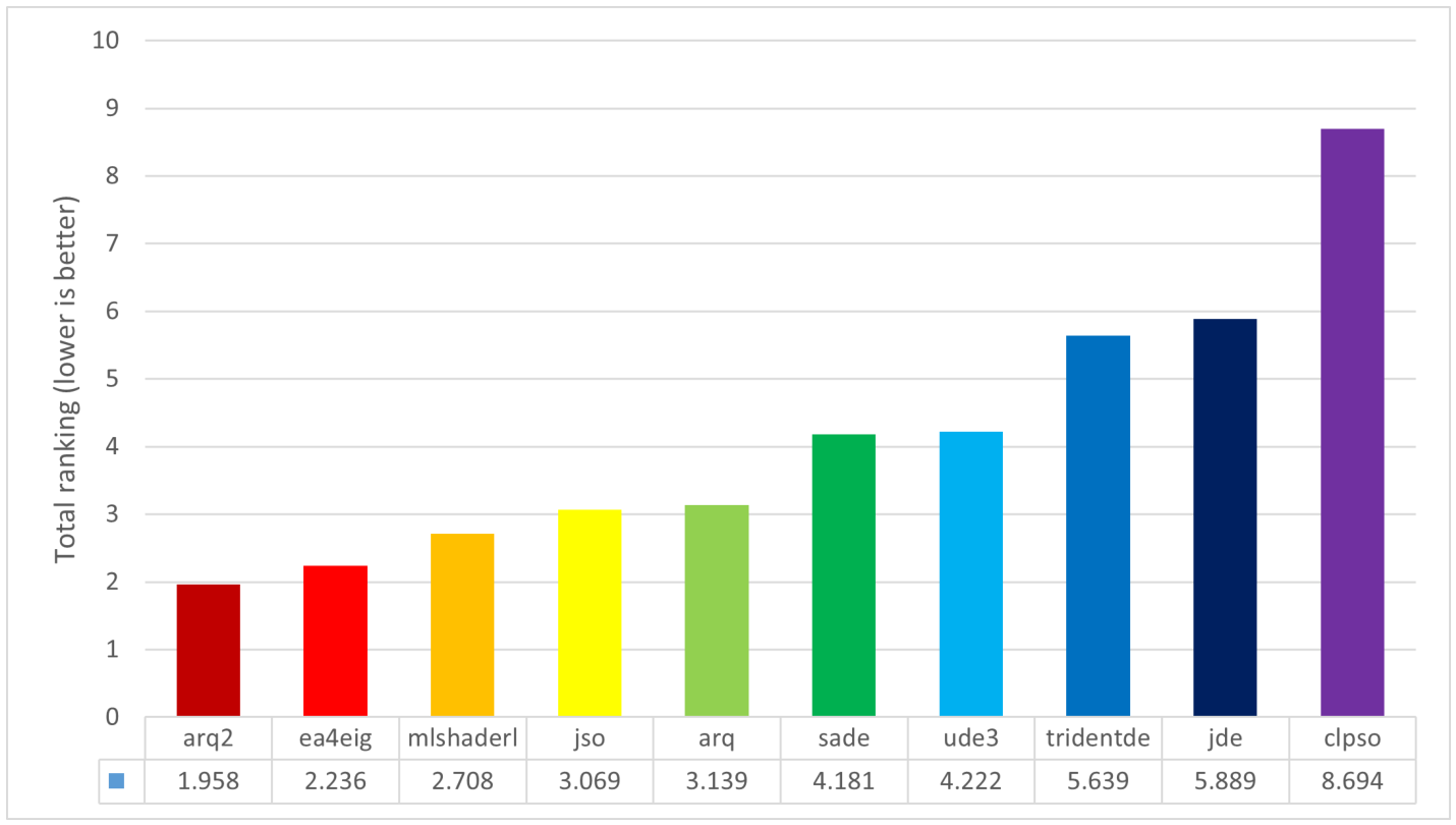
Figure 4 provides a compact visual summary of the overall comparative ranking of the evaluated methods, where lower values indicate better aggregate performance. ARQ2 attains the lowest total ranking value (1.958), followed by EA4Eig (2.236) and MLSHADE-RL (2.708), which confirms its first overall position on the complete benchmark suite. The figure also shows a clear separation between the leading group of methods and the weaker-performing algorithms, with CLPSO exhibiting the highest total ranking value. Overall, the graphical comparison is consistent with the tabulated ranking results and further supports the conclusion that ARQ2 achieves the most favorable global balance among the compared optimizers.

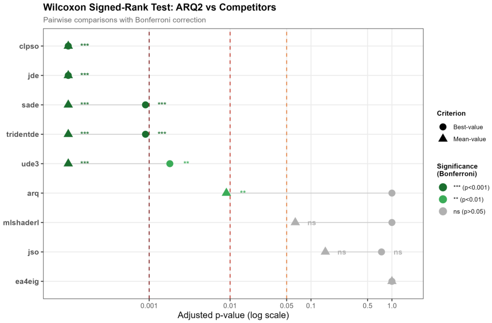
To assess whether the performance differences reported in Table 6 and Table 7 reflect genuine statistical superiority rather than sampling variability, pairwise Wilcoxon signed-rank tests were conducted between ARQ2 and each competitor across all 36 benchmark problems. Bonferroni correction was applied to the resulting p-values to control the family-wise error rate under multiple comparisons. The adjusted significance levels follow the standard notation: *** for p < 0.001, ** for p < 0.01, and ns for non-significant differences. Figure 5 summarizes the test outcomes for both the best-value and mean-value criteria on a shared logarithmic scale.

The visual evidence of Figure 5 is complemented by the exact adjusted p-values reported in

Table 9. Bonferroni-corrected Wilcoxon signed-rank p-values: ARQ2 vs. each competitor (best and mean criteria). The following notation was used: *** for p < 0.001, ** for p < 0.01, and ns for non-significant differences.

Competitor	p Value Best	p-Adjusted Best	Sig. Best	p Value Mean	p-Adjusted Mean	Sig. Mean
clpso	0	0	***	0	0	***
jde	0	0	***	0	0	***
sade	0.0001	0.0009	***	0	0	***
tridentde	0.0001	0.0009	***	0	0	***
ude3	0.0002	0.0018	**	0	0	***
arq	0.5214	1	ns	0.001	0.009	**
mlshaderl	0.1141	1	ns	0.0071	0.0639	ns
jso	0.826	0.7434	ns	0.0167	0.1503	ns
ea4eig	0.1617	1	ns	0.3402	1	ns

, which also lists the raw p-values prior to correction for completeness and reproducibility. The table separates the best-value and mean-value comparisons, allowing the significance pattern to be examined independently under the two performance criteria.

The statistical results confirm that the advantage of ARQ2 over the weaker competitors is not attributable to chance. ARQ2 is significantly superior to CLPSO, jDE, SaDE, and TRIDENT-DE under both criteria at the strictest significance level, and to UDE3 at the ** level for best values and *** for mean values. Against ARQ, the difference reaches statistical significance only in mean-value terms (p-adjusted = 0.009), which is consistent with the interpretation that ARQ2 primarily strengthens repeated-run reliability rather than peak performance. The comparisons with the three strongest rivals EA4Eig, JSO, and MLSHADE-RL remain non-significant under both criteria after Bonferroni correction, indicating that the ranking advantage of ARQ2 over these methods, while consistent in aggregate, does not translate into a statistically separable performance gap at the individual-problem level.

4.1. Empirical Convergence Complexity of ARQ2

In population-based stochastic optimization, complexity is not only associated with formal operation counts, but also with the amount of search effort required to achieve sustained improvement under a fixed evaluation budget. From this perspective, empirical convergence complexity describes how effectively a method converts its available evaluations into progressive reduction of the objective value. Its examination is relevant because final rankings alone do not show how rapidly or how consistently performance develops during the search process.

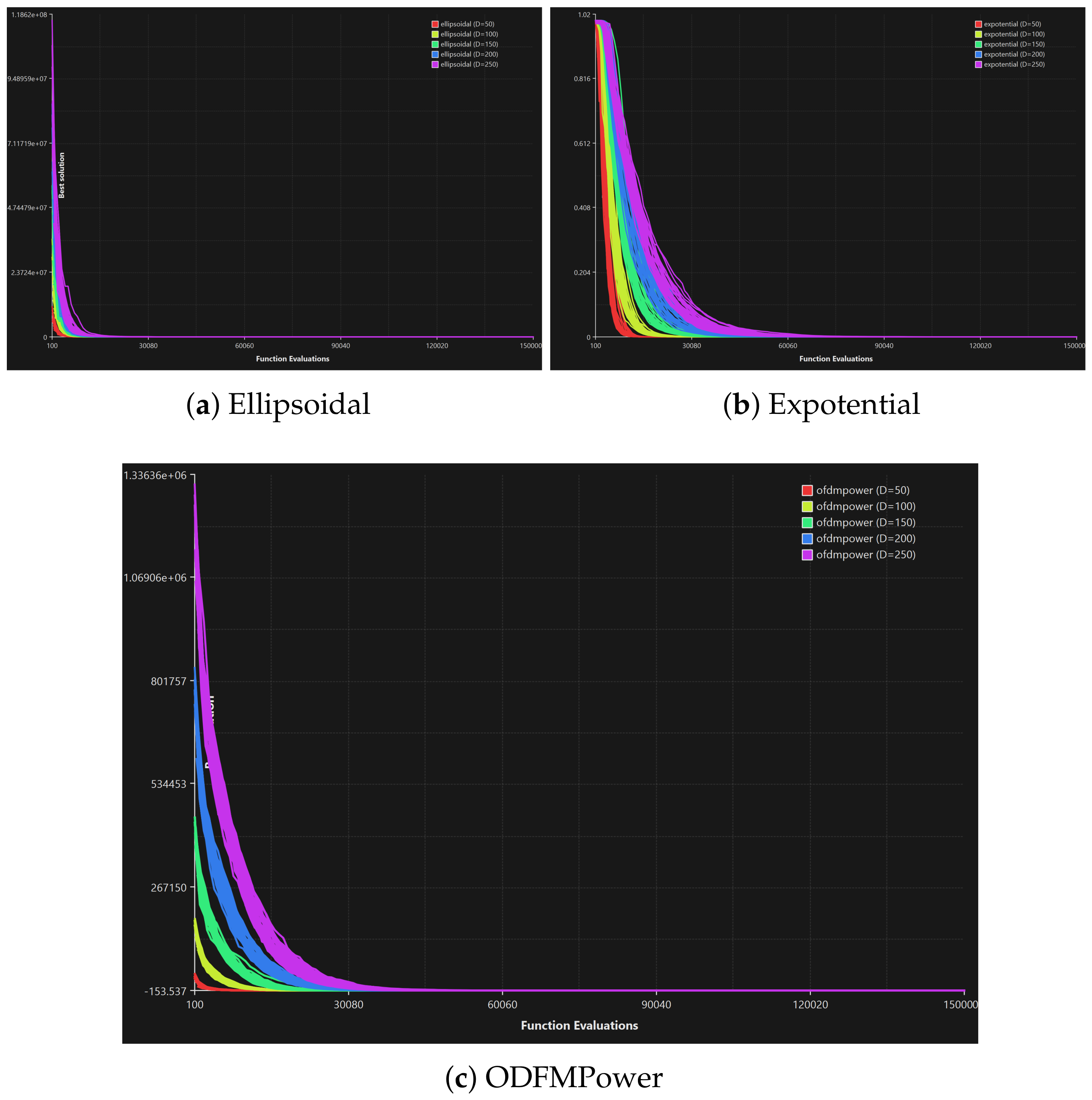
Figure 6 provides this complementary perspective through representative convergence profiles of ARQ2. The first two problems, Ellipsoidal and Exponential, belong to the non-real-world subset of the benchmark suite, whereas the third problem, OFDMPower, belongs to the real-world subset. This selection makes it possible to observe the search behavior of the proposed method on both classical synthetic landscapes and a practical application-oriented problem. The convergence traces appear visually thicker than a single smooth curve because they reflect the behavior of ARQ2 over 30 independent runs. This thickness should therefore be interpreted as an empirical indication of run-to-run variability around the general convergence trend rather than as a graphical artifact. Quantitatively, the width of the convergence band at any given evaluation count corresponds to the range between the best and worst run trajectories across the 30 independent executions, and is therefore directly related to the standard deviation of the best-so-far objective values reported in Table 3. Narrower bands indicate lower standard deviation and stronger robustness, while wider bands reflect greater run-to-run variability.

Figure 6 provides an empirical view of the practical convergence complexity of ARQ2 by showing how the objective value evolves throughout the search horizon on representative problems. In the present setting, complexity is interpreted as convergence effort, that is, the amount of search activity required for the method to generate consistent improvement under a fixed evaluation budget. The plotted trajectories suggest that ARQ2 is able to reduce the objective value progressively over a substantial portion of the optimization process, which indicates that its hybrid search mechanisms remain active beyond the earliest iterations and do not rely only on isolated opportunistic improvements.

The figure also indicates that the empirical convergence complexity of ARQ2 depends not only on the landscape type, but also on the effective dimensional burden of the problem. As dimensionality increases, the search space expands, the number of interacting decision components becomes larger, and the method must coordinate exploration and refinement in a higher-dimensional domain. For a population-based hybrid optimizer such as ARQ2, this does not simply imply a larger formal variable count, it also means that more search effort is typically required before stable improvement becomes visible. From this perspective, dimensionality contributes directly to practical optimization complexity, because the available evaluation budget must be distributed over a broader and more structurally demanding search domain.

This point is consistent with the contrast shown in Figure 6. On the two non-real-world problems, the reduction of the objective value appears more regular and more structured, which is compatible with smoother convergence behavior under the selected dimensional setting. On the real-world OFDMPower problem, the descent is comparatively slower and the convergence band is visually wider, indicating a more demanding search process and greater variability across runs. This difference is informative because it shows that the practical complexity of ARQ2 is shaped jointly by landscape structure and dimensional burden rather than by a single uniform convergence pattern over all problems.

The visual thickness of the convergence traces is itself relevant for the interpretation of complexity. Since the figure summarizes 30 independent runs, wider bands indicate stronger dispersion of the search trajectories and therefore a higher empirical cost for maintaining uniform progress. Narrower bands indicate that the available search budget is translated into more stable improvement across repeated executions. Even under this stricter perspective, the trajectories shown in Figure 6 remain coherent and do not suggest abrupt instability or immediate premature stagnation.

From a methodological standpoint, Figure 6 supports the conclusion that the additional hybridization introduced in ARQ2 does not merely increase internal procedural complexity. Instead, it appears to improve the way in which search effort is distributed between exploration and refinement, even when the dimensional and structural demands of the problem become more pronounced. The dominant computational burden remains associated with repeated objective-function evaluations, as is typical for population-based metaheuristics, while the internal control mechanisms of ARQ2 contribute to a more effective use of that evaluation budget over time. In this sense, the proposed method exhibits a favorable empirical balance between convergence efficiency, robustness, and practical computational demand.

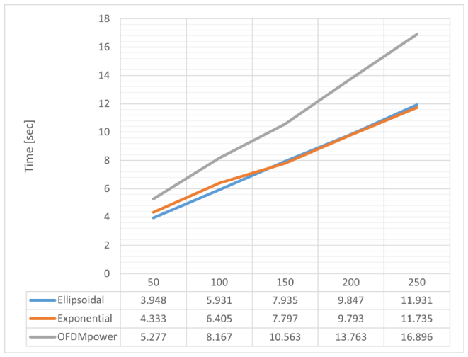
Figure 7 complements the ranking-based evidence by showing how the execution time of ARQ2 evolves as the dimensionality increases. A clear monotonic growth is observed for all three problems, which indicates that the computational burden of the proposed method increases systematically with the size of the decision space. At the same time, the growth pattern remains relatively regular over the tested dimensions, suggesting a stable empirical scalability profile rather than an abrupt computational deterioration. The two non-real-world problems, Ellipsoidal and Exponential, exhibit very similar execution-time trajectories, with values increasing from approximately 3.95 and 4.33 s at dimension 50 to about 11.74 and 11.93 s at dimension 250. In contrast, the real-world OFDMPower problem is consistently more demanding, increasing from 5.277 s at dimension 50 to 16.896 s at dimension 250. This difference is informative because it shows that the practical computational complexity of ARQ2 is shaped not only by dimensionality itself, but also by the structural characteristics of the underlying optimization problem. Consequently, the figure supports the view that ARQ2 maintains a regular empirical scaling trend as dimensionality grows, while the absolute time cost becomes higher on more demanding real-world instances.

Table 10. Mean execution time per run (seconds) of all compared methods on the complete benchmark suite.

PROBLEM	DIM	arq2	arq	clpso	ea4eig	jde	jso	mlshaderl	sade	tridentde	ude3
antennaarray	12	4.069	4.411	4.455	4.358	4.132	4.406	4.065	4.486	4.428	4.397
antennaula	10	9.877	8.714	9.927	8.873	8.716	8.671	8.695	8.76	8.683	8.681
bifunctionalcatalyst	1	0.582	0.596	0.578	0.552	0.587	0.555	0.583	0.64	0.561	0.554
ded1	120	0.269	0.192	0.293	0.194	0.305	0.204	0.308	0.233	0.166	0.151
ded2	216	0.547	0.497	0.574	0.603	0.583	0.62	0.546	0.469	0.411	0.371
eld1	6	0.072	0.07	0.068	0.028	0.066	0.031	0.053	0.12	0.036	0.028
eld2	13	0.093	0.089	0.095	0.044	0.084	0.048	0.063	0.141	0.054	0.043
eld3	15	0.104	0.095	0.109	0.052	0.097	0.057	0.079	0.149	0.062	0.051
eld4	40	0.187	0.141	0.196	0.097	0.171	0.1	0.141	0.201	0.103	0.093
eld5	140	0.358	0.204	0.397	0.189	0.631	0.207	0.811	0.255	0.172	0.15
gascycle	4	0.06	0.068	0.051	0.022	0.061	0.025	0.063	0.118	0.031	0.022
hydrothermal	96	0.325	0.193	0.362	0.174	0.659	0.189	0.953	0.251	0.163	0.141
ik6dof	6	0.087	0.087	0.092	0.047	0.079	0.05	0.063	0.138	0.054	0.047
messenger	26	0.083	0.076	0.085	0.031	0.08	0.038	0.078	0.13	0.043	0.033
ofdmpower	24	0.119	0.097	0.126	0.053	0.093	0.06	0.08	0.154	0.064	0.055
polyphase	20	0.284	0.269	0.28	0.256	0.274	0.285	0.243	0.291	0.289	0.157
potential	38	0.534	0.448	0.633	0.407	0.803	0.413	2.113	0.541	0.412	0.368
portfoliomv	10	0.074	0.071	0.075	0.03	0.064	0.036	0.05	0.124	0.038	0.039
tandem	18	0.092	0.079	0.096	0.036	0.101	0.046	0.095	0.133	0.048	0.046
tersoffb	24	1.226	1.238	1.218	1.075	1.192	0.918	1.401	1.168	1.002	0.995
tersoffc	24	1.586	1.503	1.591	1.238	1.391	1.062	1.675	1.387	1.206	1.245
transmissionpricing	126	3.147	2.948	3.092	2.541	3.34	2.79	3.054	3.014	2.961	2.667
vibratingplatform	5	0.069	0.069	0.07	0.025	0.063	0.029	0.058	0.118	0.034	0.032
wirelesscoverage	6	7.161	6.808	7.34	7.014	7.279	7.002	7.218	7.195	7.023	6.592
bucherastrigin	50	0.182	0.201	0.12	0.159	0.131	0.122	0.194	0.125	0.095	0.152
gallagher101	10	0.535	0.536	0.492	0.525	0.5	0.511	0.579	0.502	0.492	0.535
gallagher21	10	0.175	0.216	0.133	0.166	0.137	0.149	0.257	0.16	0.147	0.214
levy	24	0.127	0.129	0.064	0.093	0.066	0.076	0.166	0.07	0.064	0.102
lunacekbirastrigin	40	0.176	0.205	0.099	0.15	0.111	0.119	0.196	0.103	0.098	0.157
rotatedrosenbrock	50	0.16	0.165	0.069	0.103	0.076	0.085	0.178	0.077	0.071	0.11
schaffer	2	0.057	0.052	0.017	0.053	0.021	0.038	0.108	0.026	0.034	0.062
schwefel	16	0.094	0.111	0.045	0.085	0.053	0.097	0.153	0.057	0.049	0.112
sinusoidal	100	0.425	0.409	0.339	0.283	0.273	0.255	0.33	0.263	0.23	0.306
sinusoidal	150	0.554	0.564	0.524	0.452	0.395	0.387	0.475	0.396	0.334	0.426
test2n	200	0.485	0.372	0.294	0.66	0.265	0.453	0.357	0.255	0.173	0.246
weierstrass	50	4.324	4.309	4.908	4.437	4.624	4.264	4.301	4.468	4.483	4.431
Total		38.299	36.232	38.907	35.105	37.503	34.398	39.782	36.718	34.314	33.811

extends the runtime analysis of Figure 6 by reporting the mean execution time per run for all compared methods across the complete benchmark suite. This comparison allows the computational overhead introduced by the additional mechanisms of ARQ2 including the dual-branch architecture, roulette scheduler, quarantine stage, and micro-restart to be assessed directly against the baselines under identical hardware and budget conditions.

The results show that ARQ2 operates within a runtime range that is broadly comparable to the other methods across the majority of benchmark problems. The total accumulated time over all 36 problems amounts to 38.30 s for ARQ2, which is higher than the leanest competitors such as UDE3 (33.81 s) and TRIDENT-DE (34.31 s), but lower than MLSHADE-RL (39.78 s) and close to CLPSO (38.91 s). The overhead introduced by the additional control mechanisms of ARQ2 is therefore modest in absolute terms and does not represent a disproportionate computational cost relative to the performance gains documented in Table 6, Table 7 and Table 8.

4.2. Parameter Sensitivity Analysis of ARQ2

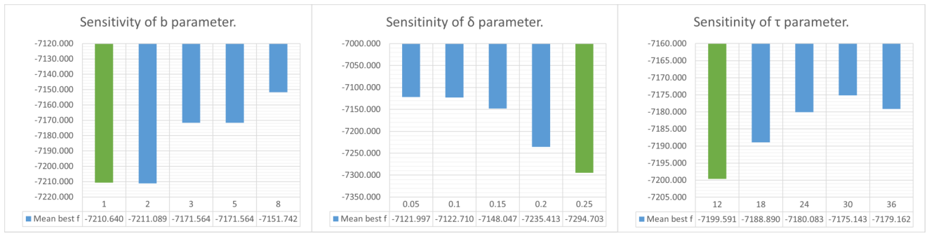
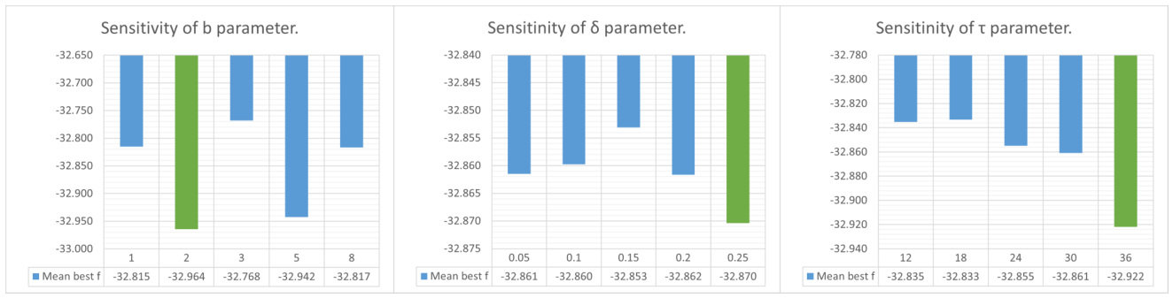
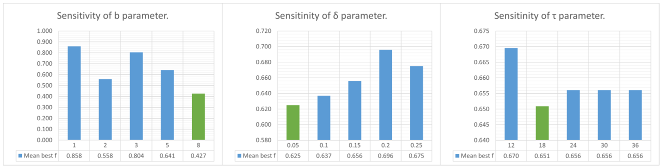
To assess the robustness of ARQ2 with respect to its control parameters, a systematic sensitivity analysis was conducted on three parameters that govern the core behavioral mechanisms of the method: the bootstrap length b, which determines the number of ARQ-only iterations enforced before competitive branch selection begins; the reset threshold $\delta$, which controls the frequency of credit resets in the roulette scheduler; and the stagnation trigger $\tau$, which sets the number of consecutive non-improving ARQ iterations required to activate the micro-restart mechanism. Each parameter was varied across five levels while the remaining parameters were held at their default values, as reported in Table 1. The analysis was performed on three representative benchmark problems that cover complementary problem characteristics: test2n (D = 200), a high-dimensional separable function; tersoffc (D = 24), a real-world molecular potential with a complex multimodal landscape; and weierstrass (D = 50), a highly multimodal function with a fractal-like structure. Mean best-value performance over 30 independent runs is reported in each case. The results are summarized in Figure 8, Figure 9 and Figure 10.

The sensitivity results across the three benchmark problems reveal a consistent pattern: the performance of ARQ2 is not critically dependent on any of the three examined parameters, and the default configuration used throughout the study remains competitive or optimal across all tested settings. The bootstrap length b exhibits minimal influence on tersoffc and moderate influence on weierstrass, where longer bootstrap values tend to yield slightly better mean performance, while b = 2 consistently produces competitive results across all three problems. The reset threshold $\delta$ shows the greatest variation on the high-dimensional test2n problem, where larger values of $\delta$, corresponding to more frequent credit resets, progressively improve mean performance, suggesting that sustained branch competition is particularly beneficial when the search space is large and the evaluation budget is relatively tight. On tersoffc, however, $\delta$ produces negligible variation across all tested levels, indicating that the scheduler behavior has little influence on problems where the landscape structure itself determines the difficulty. The stagnation trigger $\tau$ exhibits moderate sensitivity on test2n, where values in the range $\tau$ = 12 to $\tau$ = 18 tend to produce better mean outcomes than larger values, while on tersoffc and weierstrass the differences across all tested values remain small. Taken together, these results support the conclusion that ARQ2 maintains stable behavior over a reasonable range of parameter values and that its performance advantage is not contingent on precise parameter tuning. The observed variations are consistent with the general expectation that high-dimensional problems are more sensitive to scheduler and restart parameters, while lower-dimensional problems with complex landscape structure are primarily governed by the search dynamics themselves rather than by the specific control parameter settings.

4.3. Strengths and Weaknesses of the Proposed Method

The strengths and weaknesses of ARQ2 become clearer when the direct ARQ2-versus-ARQ comparison is read together with the value-based and ranking-based tables. The global picture remains favorable to the proposed method. Table 8 places ARQ2 first overall with a best total rank of 66, a mean total rank of 75, an overall rank sum of 141, and an average rank of 1.9583. This result is important because it is supported jointly by best-value and mean-value evidence rather than by a single evaluation criterion. In aggregate terms, ARQ2 therefore achieves the strongest overall balance between peak solution quality and repeated-run robustness on the complete benchmark suite. The overall first position of ARQ2 is determined by the total rank sum rather than by the count of rank-1 placements. Although EA4Eig records more rank-1 outcomes in Table 7, its total mean rank of 85 is substantially higher than that of ARQ2 at 75, indicating that EA4Eig attains top positions on fewer problems while performing less competitively on the remainder. ARQ2, by contrast, maintains a more uniformly strong position across the full benchmark suite, which is the criterion captured by the aggregate rank sum in Table 8.

A major strength of ARQ2 is its clear improvement over the original ARQ, especially in average-case behavior. Table 3 shows that, in terms of best values, ARQ2 performs better than ARQ on 10 problems, matches it on 18, and is worse on eight. The corresponding comparison in terms of mean values is substantially more favorable to ARQ2, which improves upon ARQ on 21 problems, matches it on 11, and is worse on only four. The same general tendency appears in the variability indicators, where ARQ2 attains lower standard deviation on 20 problems, equal standard deviation on 11, and higher standard deviation on only five. This pattern is consistent with the ranking tables, where the transition from ARQ to ARQ2 improves the best total rank from 81 to 66 and, even more importantly, improves the mean total rank from 145 to 75. The proposed extension therefore appears to strengthen ARQ primarily at the level of reliability, stability, and repeated-run competitiveness, rather than only at the level of isolated favorable outcomes. The cases where ARQ2 yields a worse best value than ARQ can be attributed to the inherent cost of hybridization. By distributing evaluations between two branches under the roulette scheduler, ARQ2 allocates a fraction of its computational budget to the IDE branch, which may divert search effort away from the most productive region on problems where the ARQ search dynamic alone would have been sufficient. This trade-off is the expected consequence of designing for robustness across a heterogeneous benchmark suite rather than for peak performance on any specific problem class.

Another important strength of ARQ2 is its positional consistency across the full benchmark collection. In Table 6, ARQ2 achieves 25 rank-1 placements and 29 top-three placements, which gives it the lowest best-based total rank among all compared methods. In Table 7, it records 31 top-three placements and no placements in the lower-performance tail of the ranking distribution, again yielding the best total rank. This is a particularly strong feature of the method: ARQ2 is not merely competitive because of a limited number of exceptional runs, but because it remains close to the leading positions over a large portion of the benchmark suite. The same conclusion is supported by Table 6 and Table 7. ARQ2 reaches the best recorded final value on 25 problems when ties are counted, which is the highest count among all methods, while in mean-value terms it remains among the strongest methods even though the competition becomes more evenly distributed.

When the benchmark is viewed through its real-world and non-real-world components, an additional strength of ARQ2 becomes visible. Over the real-world subset introduced in Section 4, ARQ2 obtains the best aggregate behavior in both criteria, with a best-rank average of 2.0417 and a mean-rank average of 1.9583. This is a meaningful result because the practical relevance of the study depends heavily on these application-oriented problems. At the same time, the non-real-world subset reveals a more nuanced picture. ARQ2 remains the strongest method in best-value terms on the classical benchmark functions, with an average best rank of 1.4167, but it is slightly surpassed by EA4Eig in mean-value terms, where ARQ2 attains an average mean rank of 2.3333 against 2.0833 for EA4Eig. This indicates that ARQ2 retains strong peak performance on the synthetic part of the benchmark, while its average behavior on that subset is not uniformly dominant against the strongest competitor.

This last point leads directly to the main weaknesses of the proposed method. The first weakness is that ARQ2 is not the per-problem leader in mean-value behavior as often as its overall first position might initially suggest. In Table 7, EA4Eig records 19 rank-1 placements and JSO records 17, whereas ARQ2 records 15. The overall advantage of ARQ2 therefore comes less from dominating every individual problem and more from maintaining a more uniform competitive profile across the suite. The second weakness is that a number of difficult problems remain clearly challenging. In best-based ranking terms, relatively weak placements are observed on tersoffb and vibratingplatform, where ARQ2 receives rank 6, and on ded1, ded2, eld5, hydrothermal, and rotatedrosenbrock, where it receives rank 4. In mean-based terms, the most visible weakness appears on sinusoidal, where ARQ2 receives rank 6, while eld4, hydrothermal, transmissionpricing, and rotatedrosenbrock remain at rank 4. These cases indicate that ARQ2 still encounters difficulties on selected high-dimensional engineering instances and on some structurally demanding synthetic landscapes.

The comparison with the strongest competitors also remains instructive. EA4Eig is the closest overall rival of ARQ2 and appears particularly strong in mean-value performance on the non-real-world subset. JSO remains highly competitive on selected problems and retains a large number of rank-1 outcomes, especially in value-based comparisons. MLSHADE-RL, although not first overall, also maintains consistently strong aggregate positions. Against this backdrop, the advantage of ARQ2 should not be interpreted as universal dominance, but as the most favorable overall compromise among the compared methods. Its central strength lies in combining strong best-case performance, strong aggregate mean behavior, and a marked improvement over ARQ in repeated-run reliability. Its central weakness is that this advantage is not uniform across all problem classes, especially on some demanding real-world scheduling and design problems and on a few difficult non-real-world functions. Even so, the evidence of the tables supports the conclusion that ARQ2 offers the most balanced general-purpose performance profile in the present study.

5. Conclusions

This study presented ARQ2 and evaluated its performance on a heterogeneous benchmark suite of 36 continuous optimization problems, comprising both real-world and classical instances. The experimental results confirm that ARQ2 achieves the strongest overall aggregate performance among the ten compared methods, attaining the lowest total rank sum of 141 and an average rank of 1.958 across best-value and mean-value criteria jointly. Compared to its predecessor ARQ, the proposed extension improves mean-value performance on 21 out of 36 problems and attains lower solution variability on 20 problems, demonstrating that the primary contribution of ARQ2 lies in strengthening repeated-run reliability rather than producing isolated favorable outcomes.

At the same time, the results make clear that ARQ2 is not universally superior across all problem classes, and that strong competitors such as EA4Eig, MLSHADE-RL, and JSO remain highly competitive on selected problems. The present findings should therefore be interpreted as evidence of strong general competitiveness and improved robustness, while also identifying specific problem classes where further refinement remains warranted. In this sense, the current study establishes a solid basis for the next stage of methodological development of the ARQ design line.

References

1. Rios, L.M.; Sahinidis, N.V. Derivative-free optimization: A review of algorithms and comparison of software implementations. J. Glob. Optim. 2013, 56, 1247–1293. [Google Scholar] [CrossRef]
2. Coello Coello, C.A. Theoretical and numerical constraint-handling techniques used with evolutionary algorithms: A survey of the state of the art. Comput. Methods Appl. Mech. Eng. 2002, 191, 1245–1287. [Google Scholar] [CrossRef]
3. Kirkpatrick, S.; Gelatt, C.D., Jr.; Vecchi, M.P. Optimization by simulated annealing. Science 1983, 220, 671–680. [Google Scholar] [CrossRef]
4. Kennedy, J.; Eberhart, R. Particle swarm optimization. In Proceedings of ICNN’95-International Conference on Neural Networks; IEEE: Piscataway, NJ, USA, 1995; Volume 4, pp. 1942–1948. [Google Scholar] [CrossRef]
5. Hansen, N.; Ostermeier, A. Completely derandomized self-adaptation in evolution strategies. Evol. Comput. 2001, 9, 159–195. [Google Scholar] [CrossRef]
6. Dorigo, M.; Maniezzo, V.; Colorni, A. Ant system: Optimization by a colony of cooperating agents. IEEE Trans. Syst. Man Cybern.-Part B Cybern. 1996, 26, 29–41. [Google Scholar] [CrossRef]
7. Glover, F. Tabu search-Part I. ORSA J. Comput. 1989, 1, 190–206. [Google Scholar] [CrossRef]
8. Glover, F.; Laguna, M.; Martí, R. Scatter search. In Advances in Evolutionary Computing; Ghosh, A., Tsutsui, S., Eds.; Springer: Berlin/Heidelberg, Germany, 2003; pp. 519–537. [Google Scholar] [CrossRef]
9. Geem, Z.W.; Kim, J.H.; Loganathan, G.V. A new heuristic optimization algorithm: Harmony search. Simulation 2001, 76, 60–68. [Google Scholar] [CrossRef]
10. Karaboga, D.; Basturk, B. A powerful and efficient algorithm for numerical function optimization: Artificial bee colony (ABC) algorithm. J. Glob. Optim. 2007, 39, 459–471. [Google Scholar] [CrossRef]
11. Yang, X.-S. Firefly algorithm, stochastic test functions and design optimisation. Int. J. Bio-Inspired Comput. 2010, 2, 78–84. [Google Scholar] [CrossRef]
12. Yang, X.-S.; Deb, S. Cuckoo search via Lévy flights. In 2009 World Congress on Nature Biologically Inspired Computing (NaBIC); IEEE: Piscataway, NJ, USA, 2009; pp. 210–214. [Google Scholar] [CrossRef]
13. Yang, X.-S. A new metaheuristic bat-inspired algorithm. In Nature Inspired Cooperative Strategies for Optimization (NICSO 2010); Springer: Berlin/Heidelberg, Germany, 2010; pp. 65–74. [Google Scholar] [CrossRef]
14. Rao, R.V.; Savsani, V.J.; Vakharia, D.P. Teaching-learning-based optimization: A novel method for constrained mechanical design optimization problems. Comput.-Aided Des. 2011, 43, 303–315. [Google Scholar] [CrossRef]
15. Rashedi, E.; Nezamabadi-Pour, H.; Saryazdi, S. GSA: A gravitational search algorithm. Inf. Sci. 2009, 179, 2232–2248. [Google Scholar] [CrossRef]
16. Mirjalili, S.; Mirjalili, S.M.; Lewis, A. Grey wolf optimizer. Adv. Eng. Softw. 2014, 69, 46–61. [Google Scholar] [CrossRef]
17. Mirjalili, S.; Lewis, A. The whale optimization algorithm. Adv. Eng. Softw. 2016, 95, 51–67. [Google Scholar] [CrossRef]
18. Simon, D. Biogeography-based optimization. IEEE Trans. Evol. Comput. 2008, 12, 702–713. [Google Scholar] [CrossRef]
19. Mehrabian, A.R.; Lucas, C. A novel numerical optimization algorithm inspired from weed colonization. Ecol. Inform. 2006, 1, 355–366. [Google Scholar] [CrossRef]
20. Eusuff, M.M.; Lansey, K.E. Optimization of water distribution network design using the shuffled frog leaping algorithm. J. Water Resour. Plan. Manag. 2003, 129, 210–225. [Google Scholar] [CrossRef]
21. Krasnogor, N.; Smith, J. A tutorial for competent memetic algorithms: Model, taxonomy, and design issues. IEEE Trans. Evol. Comput. 2005, 9, 474–488. [Google Scholar] [CrossRef]
22. Larrañaga, P.; Lozano, J.A. (Eds.) Estimation of Distribution Algorithms: A New Tool for Evolutionary Computation; Springer: Berlin/Heidelberg, Germany, 2002. [Google Scholar] [CrossRef]
23. Storn, R.; Price, K. Differential evolution: A simple and efficient heuristic for global optimization over continuous spaces. J. Glob. Optim. 1997, 11, 341–359. [Google Scholar] [CrossRef]
24. Ahmad, M.F.; Isa, N.A.M.; Lim, W.H.; Ang, K.M. Differential evolution: A recent review based on state-of-the-art works. Alex. Eng. J. 2022, 61, 3831–3872. [Google Scholar] [CrossRef]
25. Das, S.; Suganthan, P.N. Differential evolution: A survey of the state-of-the-art. IEEE Trans. Evol. Comput. 2011, 15, 4–31. [Google Scholar] [CrossRef]
26. Zhang, J.; Sanderson, A.C. JADE: Adaptive differential evolution with optional external archive. IEEE Trans. Evol. Comput. 2009, 13, 945–958. [Google Scholar] [CrossRef]
27. Wang, Y.; Cai, Z.; Zhang, Q. Differential evolution with composite trial vector generation strategies and control parameters. IEEE Trans. Evol. Comput. 2011, 15, 55–66. [Google Scholar] [CrossRef]
28. Tanabe, R.; Fukunaga, A. Success-history based parameter adaptation for differential evolution. In 2013 IEEE Congress on Evolutionary Computation (CEC); IEEE: Piscataway, NJ, USA, 2013; pp. 71–78. [Google Scholar] [CrossRef]
29. Tanabe, R.; Fukunaga, A.S. Improving the search performance of SHADE using linear population size reduction. In 2014 IEEE Congress on Evolutionary Computation (CEC); IEEE: Piscataway, NJ, USA, 2014; pp. 1658–1665. [Google Scholar] [CrossRef]
30. Charilogis, V.; Tsoulos, I.G.; Gianni, A.M.; Tsalikakis, D. ARQ: A cohesive optimization design for stable performance on noisy landscapes. Appl. Sci. 2025, 15, 12180. [Google Scholar] [CrossRef]
31. Bujok, P.; Kolenovský, P. Eigen crossover in cooperative model of evolutionary algorithms applied to CEC 2022 single objective numerical optimisation. In 2022 IEEE Congress on Evolutionary Computation (CEC); IEEE: Piscataway, NJ, USA, 2022; pp. 1–8. [Google Scholar] [CrossRef]
32. Biedrzycki, R. Analysis and simplification of the winner of the CEC 2022 optimization competition on single objective bound constrained search. Evol. Comput. 2025, 1–18. [Google Scholar] [CrossRef]
33. Brest, J.; Maučec, M.S.; Bošković, B. Single objective real-parameter optimization: Algorithm jSO. In 2017 IEEE Congress on Evolutionary Computation (CEC); IEEE: Piscataway, NJ, USA, 2017; pp. 1311–1318. [Google Scholar] [CrossRef]
34. Brest, J.; Greiner, S.; Bošković, B.; Mernik, M.; Žumer, V. Self-adapting control parameters in differential evolution: A comparative study on numerical benchmark problems. IEEE Trans. Evol. Comput. 2006, 10, 646–657. [Google Scholar] [CrossRef]
35. Chauhan, D.; Trivedi, A.; Shivani. A multi-operator ensemble LSHADE with restart and local search mechanisms for single-objective optimization. arXiv 2024. [Google Scholar] [CrossRef]
36. Liang, J.J.; Qin, A.K.; Suganthan, P.N.; Baskar, S. Comprehensive learning particle swarm optimizer for global optimization of multimodal functions. IEEE Trans. Evol. Comput. 2006, 10, 281–295. [Google Scholar] [CrossRef]
37. Charilogis, V.; Tsoulos, I.G.; Gianni, A.M. TRIDENT-DE: Triple-operator differential evolution with adaptive restarts and greedy refinement. Future Internet 2025, 17, 488. [Google Scholar] [CrossRef]
38. Trivedi, A.; Chauhan, D. UDE-III: An enhanced unified differential evolution algorithm for constrained optimization problems. arXiv 2024. [Google Scholar] [CrossRef]
39. Qin, A.K.; Huang, V.L.; Suganthan, P.N. Differential evolution algorithm with strategy adaptation for global numerical optimization. IEEE Trans. Evol. Comput. 2009, 13, 398–417. [Google Scholar] [CrossRef]
40. Al-Roomi, A.R. IEEE Congresses on Evolutionary Computation Repository; Dalhousie University, Electrical and Computer Engineering: Halifax, NS, Canada, 2015. [Google Scholar]
41. Elsayed, S.M.; Sarker, R.A.; Essam, D.L. Differential evolution with multiple strategies for solving CEC2011 real-world numerical optimization problems. In 2011 IEEE Congress on Evolutionary Computation; IEEE: Piscataway, NJ, USA, 2011; pp. 1041–1048. [Google Scholar] [CrossRef]
42. Chowdhury, A.; Giri, R.; Ghosh, A.; Das, S.; Abraham, A.; Snášel, V. Linear antenna array synthesis using fitness-adaptive differential evolution algorithm. In 2010 IEEE Congress on Evolutionary Computation; IEEE: Piscataway, NJ, USA, 2010; pp. 1–8. [Google Scholar] [CrossRef]
43. Hofer, E.P. Optimization of bifunctional catalysts in tubular reactors. J. Optim. Theory Appl. 1976, 18, 379–393. [Google Scholar] [CrossRef]
44. Luus, R.; Dittrich, J.; Keil, F.J. Multiplicity of solutions in the optimization of a bifunctional catalyst blend in a tubular reactor. Can. J. Chem. Eng. 1992, 70, 780–785. [Google Scholar] [CrossRef]
45. Luus, R.; Bojkov, B. Global optimization of the bifunctional catalyst problem. Can. J. Chem. Eng. 1994, 72, 160–163. [Google Scholar] [CrossRef]
46. Aghajarian, M.; Kiani, K. Inverse kinematics solution of PUMA 560 robot arm using ANFIS. In 2011 8th International Conference on Ubiquitous Robots and Ambient Intelligence; IEEE: Piscataway, NJ, USA, 2011; pp. 574–578. [Google Scholar] [CrossRef]
47. Schlueter, M.; Neshat, M.; Wahib, M.; Munetomo, M.; Wagner, M. GTOPX space mission benchmarks. SoftwareX 2021, 14, 100666. [Google Scholar] [CrossRef]
48. He, H.; Stoica, P.; Li, J. Designing unimodular sequence sets with good correlations—Including an application to MIMO radar. IEEE Trans. Signal Process. 2009, 57, 4391–4405. [Google Scholar] [CrossRef]
49. Jones, J.E. On the determination of molecular fields. II. From the equation of state of a gas. Proc. R. Soc. A Math. Phys. Eng. Sci. 1924, 106, 463–477. [Google Scholar] [CrossRef]
50. Markowitz, H. Portfolio selection. J. Financ. 1952, 7, 77–91. [Google Scholar] [CrossRef]
51. Tersoff, J. New empirical approach for the structure and energy of covalent systems. Phys. Rev. B 1988, 37, 6991–7000. [Google Scholar] [CrossRef]
52. Tersoff, J. Modeling solid-state chemistry: Interatomic potentials for multicomponent systems. Phys. Rev. B 1989, 39, 5566–5568. [Google Scholar] [CrossRef]
53. Garver, L.L. Transmission network estimation using linear programming. IEEE Trans. Power Appar. Syst. 1970, PAS-89, 1688–1697. [Google Scholar] [CrossRef]
54. Schweppe, F.C.; Caramanis, M.C.; Tabors, R.D.; Bohn, R.E. Spot Pricing of Electricity; Springer: Berlin/Heidelberg, Germany, 1988. [Google Scholar] [CrossRef]
55. Calles-Esteban, F.; Olmedo, A.A.; Hellín, C.J.; Valledor, A.; Gómez, J.; Tayebi, A. Optimizing antenna positioning for enhanced wireless coverage: A genetic algorithm approach. Sensors 2024, 24, 2165. [Google Scholar] [CrossRef]
56. Varelas, K.; Ait El Hara, O.; Brockhoff, D.; Hansen, N.; Nguyen, D.M.; Tušar, T.; Auger, A. Benchmarking large-scale continuous optimizers: The bbob-largescale testbed, a COCO software guide and beyond. Appl. Soft Comput. 2020, 97, 106737. [Google Scholar] [CrossRef]
57. Jamil, M.; Yang, X.-S. A literature survey of benchmark functions for global optimisation problems. Int. J. Math. Model. Numer. Optim. 2013, 4, 150–194. [Google Scholar] [CrossRef]
58. Ali, M.M.; Khompatraporn, C.; Zabinsky, Z.B. A numerical evaluation of several stochastic algorithms on selected continuous global optimization test problems. J. Glob. Optim. 2005, 31, 635–672. [Google Scholar] [CrossRef]
Figure 1. Overall workflow of ARQ2.
Symmetry 18 00844 g001
Figure 2. Roulette-based branch scheduling in ARQ2.
Symmetry 18 00844 g002
Figure 3. IDE branch update in ARQ2.
Symmetry 18 00844 g003
Figure 4. Total ranking combining best and mean across 10 algorithms.
Symmetry 18 00844 g004
Figure 5. Bonferroni-corrected Wilcoxon signed-rank test results: ARQ2 vs. each competitor (best and mean criteria).
Symmetry 18 00844 g005
Figure 6. Empirical convergence profiles of ARQ2 over 30 independent runs on representative benchmark problems with different landscape characteristics.
Symmetry 18 00844 g006
Figure 7. Execution time of ARQ2 as a function of dimensionality on three problems.
Symmetry 18 00844 g007
Figure 8. Test2n problem. Dimension 200. (best value: green color) problem. Dimension 200.
Symmetry 18 00844 g008
Figure 9. Tersoffc problem. (best value: green color) problem.
Symmetry 18 00844 g009
Figure 10. Weiresrtrass problem. Dimension 50. (best value: green color) problem. Dimension 50.
Symmetry 18 00844 g010