Modeling and Reliability Assessment of Wind Farm Energy Production Considering Wake Effects and Performance Degradation

Abstract

To address limitations in existing wind farm energy production calculation and reliability assessment—including simplified wake effects, neglected performance degradation, and over-reliance on large-sample data—this study proposes a belief-reliability modeling framework integrating wake dynamics, performance degradation, and dual-uncertainty analysis. It quantifies wake-induced wind speed deficits, captures the degradation of the wind energy utilization coefficient, and models external and internal uncertainties, with external uncertainty referring to wind speed, which follows a Weibull distribution, and internal uncertainty referring to the degradation of the wind energy utilization coefficient, which falls into the category of epistemic uncertainty. By integrating belief reliability theory, a power generation demand reliability metric is developed to enable accurate assessment for data-limited wind farms, and case studies confirm that the framework improves life cycle energy production and reliability prediction accuracy while supporting wind farm design, maintenance, and energy planning.

1. Introduction

As a cornerstone of the renewable energy transition, wind energy has garnered global attention for its clean, sustainable nature and vast reserves, making wind farms a critical infrastructure for addressing energy security and climate change challenges. With the rapid expansion of large-scale and multi-phase wind farm projects worldwide, accurately quantifying wind farm energy production has become essential to ensuring operational efficiency, economic viability, and long-term energy supply stability.

Currently, existing methods for calculating wind farm energy production can be broadly categorized into two types: statistical models and physical models. Statistical models, such as Auto-Regressive Moving Average (ARMA) models and artificial neural network (ANN) models, rely on historical wind speed and energy data to establish predictive relationships. For instance, ARMA models capture temporal correlations in wind speed sequences to forecast short-term energy output [1], while ANN models handle nonlinear relationships between wind conditions and energy production [2]. Physical models, on the other hand, focus on the intrinsic energy conversion process of wind turbines and the spatial interactions between turbines. Representative approaches include the Jensen wake model [3] and its extended 3D Jensen–Gaussian wake model [4], which describe wind speed deficits caused by upstream turbine wakes and calculate energy production by integrating turbine aerodynamic characteristics. Commercial software such as WAsP 12.5 [5], Windfarmer 5.0, and WindPro 3.8 [6] also adopt physical principles to simulate wind farm energy production under different terrain and wind conditions. While these methods provide valuable tools for energy calculation, they often simplify or ignore dynamic lifecycle factors such as wake effects and performance degradation.

In reality, wind farm energy production declines over time due to degradation factors, requiring uncertainty quantification and degradation characterization for accurate prediction [7]. These factors introduce aleatory and epistemic uncertainties, rendering static calculation methods inadequate. A robust energy model must thus integrate degradation dynamics and uncertainty analysis to capture real lifecycle performance.

A critical gap in existing research is the limited sample size for reliability assessment in wind farm energy calculations. Traditional reliability assessment methods, such as probabilistic reliability analysis, require large volumes of failure data to estimate component reliability parameters [8]. However, wind farms—especially those with new turbine models or in complex terrains—often lack sufficient historical data, leading to inaccurate reliability evaluations.

To address the aforementioned challenges, uncertainty theory and belief-reliability theory have emerged as powerful tools for wind farm system modeling. Uncertainty theory, which differentiates between aleatory and epistemic uncertainties, provides a framework for quantifying unknowns arising from limited data or incomplete knowledge [9]. For wind farms, this theory enables the characterization of wind-speed randomness using probability distributions and turbine failure count ambiguity using uncertainty distributions [10]. Building on this, belief reliability theory [11] goes beyond traditional probabilistic reliability. This theory explicitly accounts for both types of uncertainties, making it well-suited for small-sample scenarios [12]. For example, belief reliability metrics can quantify the probability that wind farm energy production meets demand thresholds [13], even with limited failure data, by combining chance theory for uncertainty propagation.

This study focuses on developing a belief reliability modeling method for wind farm systems. By integrating wake effects and performance degradation into energy calculations, this method aims to address the limitations of existing models and to provide a robust tool for life-cycle reliability assessment. The remainder of this paper is structured as follows: Section 2 elaborates on the literature review concerning wake effect modeling, performance degradation analysis, and reliability assessment methodologies. Section 3 constructs the wind farm energy production model that incorporates wake effects, detailing the Jensen wake model and the multi-wake superposition mechanism. Section 4 establishes a performance-degradation model for the wind energy utilization coefficient based on uncertain processes. Section 5 conducts a case study to validate the proposed framework. Finally, Section 6 presents the discussion and conclusions, along with recommendations for future research.

Comparison with conventional probabilistic reliability methods. Unlike traditional probabilistic reliability assessment that relies on large-sample failure data and assumes known probability distributions, our belief reliability framework offers three distinct advantages: (i) handling of epistemic uncertainty—the Liu process quantifies what is unknown due to limited data, whereas probabilistic methods would either ignore it or make arbitrary distributional assumptions; (ii) small-sample validity—the moment estimation method (Section 4.2) remains consistent with as few as 5–10 data points, while maximum likelihood estimation would produce unreliable confidence intervals; (iii) unified uncertainty propagation—the opportunity measure $\mathcal{M}$, defined on the product space of probability and uncertainty measures, allows simultaneous treatment of random wind speed and epistemic degradation, which probabilistic methods cannot accommodate without double-loop simulation.

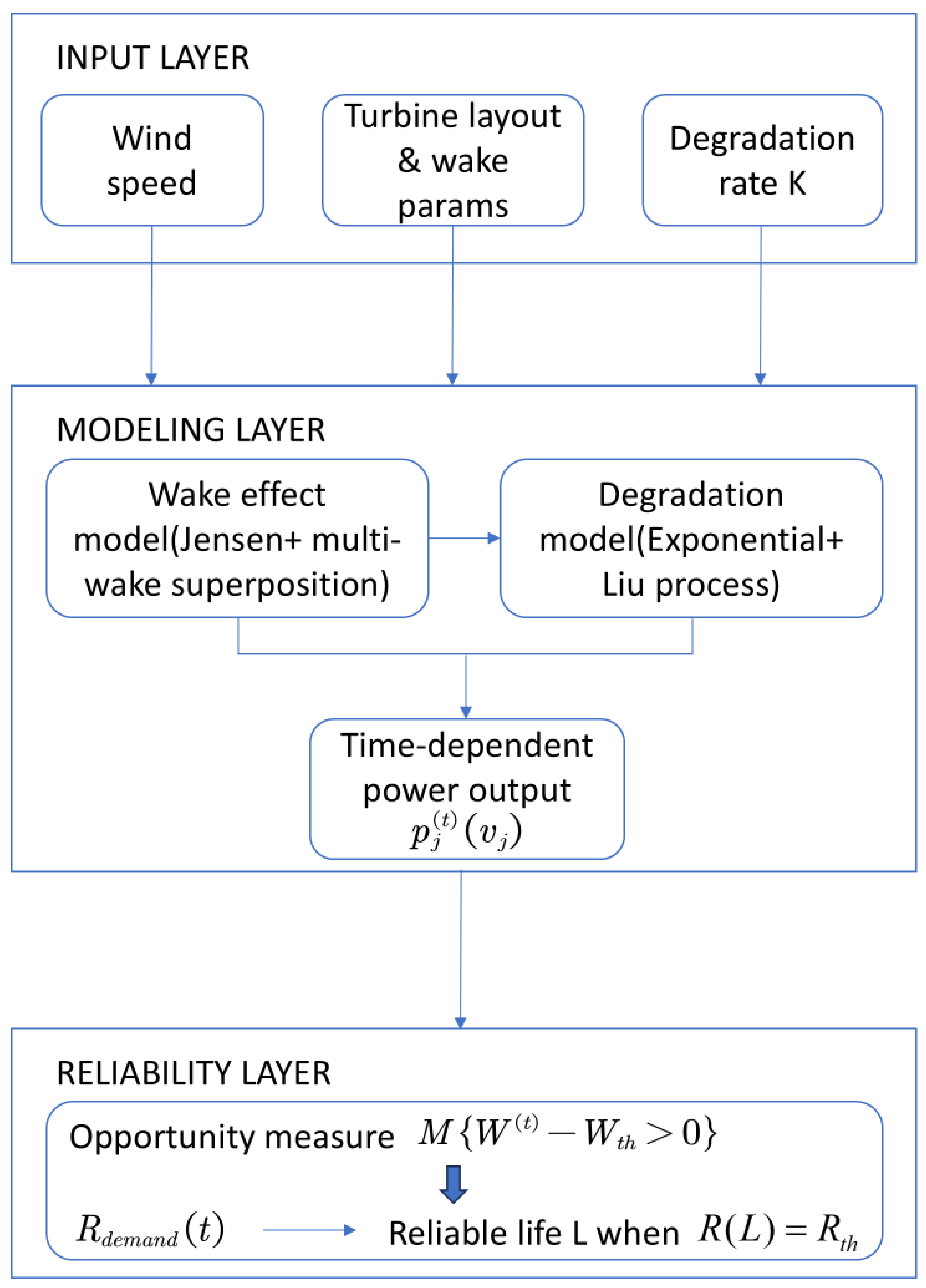
As illustrated in Figure 1, the proposed framework consists of three sequential layers that propagate uncertainties from input to reliability output.

Schematic of the three-layer belief reliability modeling framework for wind farm energy production. The framework comprises three layers. The input layer distinguishes aleatory uncertainty (wind speed following a Weibull distribution) from epistemic uncertainty (degradation of the wind energy utilization coefficient modeled by a Liu process). The modeling layer integrates wake effects (Jensen model with multi-wake superposition) and time-dependent degradation (exponential decay with uncertain differential equation). The reliability layer computes the belief reliability metric $R_{demand}\left(t\right)$ using the opportunity measure and defines the reliable life L.

2. Wind Farm Power Generation Model

The function of a wind farm is to capture the kinetic energy of wind and convert it into usable electrical energy. The power generation and output of a wind farm are important performance indicators for describing the functionality of the wind farm system, where total energy production is the long-term performance of the wind farm and the key performance focus of this paper.

2.1. Jensen Wake Model

When constructing interdisciplinary equations for wind farm power generation, the wake effect is an important consideration. The wake effect mainly describes the phenomenon of wind turbines obtaining energy from the wind while forming a downstream wake zone where the wind speed decreases. If there is a wind turbine located in the wake area of the upstream wind turbine downstream, its input wind speed will be lower than that of the upstream wind turbine. The wake effect causes uneven distribution of wind speed within the wind farm, affecting the operation status of each wind turbine unit in the wind farm, further affecting the operating conditions and output power of the wind farm, and is influenced by factors such as wind farm layout structure, wind turbine diameter, thrust coefficient, wind speed, and direction. According to research, power generation loss caused by wake effects is generally 5% to 15%, and sometimes as high as 30% to 40%. Recent benchmarking studies confirm that wake losses remain one of the largest sources of uncertainty in wind farm energy yield assessment, with pre-construction estimates often deviating from operational values by 2–6 percentage points [14].

Introduced by Jensen (1983), this wake model has become a standard approach for characterizing turbine-turbine aerodynamic interactions within wind farms. The wind speed in the wake can be calculated using the following formula:

$$v_d=v_0\left(1-{\displaystyle \frac{2a}{1+\frac{kD}{r_0}}}\right),$$

(1)

where $v_0$ is the upstream wind speed not affected by the wind turbine. $r_0$ is the radius of the wind turbine rotor. $k$ is a constant representing the wake diffusion angle (usually ranging from 0.05 to 0.1). $D$ is the horizontal distance from the wind turbine to the point considered in the wake. $r$ is the wake radius, which increases with distance $x$, and $r=r_0+kD$. The axial induction factor $a={\displaystyle \frac{1}{2}}(1-\sqrt{1-C_T})$ is a dimensionless parameter that characterizes the degree to which the wind turbine extracts energy from the wind.

While more sophisticated wake models exist (e.g., CFD-based RANS simulations, dynamic wake meandering models), the Jensen model remains the industry standard for wind farm energy assessment. For the purpose of reliability analysis, where uncertainty propagation is the primary focus, the analytical tractability of the Jensen model outweighs marginal gains in wake prediction accuracy. Moreover, the error introduced by Jensen’s conical wake assumption (k ≈ 0.05–0.1) is typically within 3–5% of more complex models, which is negligible compared to the uncertainty from performance degradation.

2.2. Single and Multiple Wake Superposition

In the wake effect, the wake spreads in a conical shape, and the wind speed attenuation mainly occurs along the direction of the wind. When the downstream fan impeller overlaps with the upstream fan’s wake, the weighted average of its wind speed can be estimated based on the proportion of the overlap area between the upstream wake and the downstream fan impeller in the total impeller area.

For partial coverage, assuming the radius of the fan impeller is $r_0$, the radius of the projection of the wake model at x is $r_z\left(x\right)$, and the distance between the centers of the two circles is d.

According to the formula for intersecting the areas of two circles, the coverage area is

$$\begin{array}{c}A=r_0^2{\cos }^{-1}\left({\displaystyle \frac{d^2+r_0^2-r_z{\left(x\right)}^2}{2d{r}_0}}\right)+r_z{\left(x\right)}^2{\cos }^{-1}\left({\displaystyle \frac{d^2+r_z{\left(x\right)}^2-r_0^2}{2d{r}_z\left(x\right)}}\right)\\ -{\displaystyle \frac{1}{2}}\sqrt{\left(-d+r_0+r_z\left(x\right)\right)\left(d+r_0-r_z\left(x\right)\right)\left(d-r_0+r_z\left(x\right)\right)\left(d+r_0+r_z\left(x\right)\right)}.\end{array}$$

(2)

The area weighting coefficient is defined as

$$\beta ={\displaystyle \frac{A}{\pi r_0^2}},$$

(3)

indicating the proportion of the downstream fan area covered by the upstream fan wake. When fully covered, $\beta =1$; when partially covered, $\beta <1$.

The effective inflow wind speed of fan i (only affected by the wake of fan j) is as follows:

$$v_i^j={\beta }_i\cdot u_j\left(x,y,z\right)+\left(1-{\beta }_i\right)\cdot v_o.$$

(4)

In large wind farms, wind turbines are usually arranged in an array (such as a grid), and downstream wind turbines may not only be located in the wake of a single upstream wind turbine, but also within the wake influence range of multiple upstream wind turbines simultaneously. These wake interactions, merging, and stacking from different upstream wind turbines form a larger, more complex, and far-reaching composite wake region (with lower wind speeds and stronger turbulence). The practical significance of accurate wake modeling has been demonstrated in recent studies on offshore wind farm stability analysis, where wake-induced differences in operating conditions among turbines significantly affect system-wide dynamic characteristics [15].

This paper uses the kinetic energy loss superposition method to calculate the wind speed under the influence of multiple wake superposition. Therefore, the effective wind speed of wind turbine unit i after being affected by the wake effect of the upstream J wind turbine units is as follows:

$$v_i=\sqrt{v_0^2-\underset{j=1}{\stackrel{J}{\Sigma }}\left(v_j^2-v_i^{j2}\right)}.$$

(5)

2.3. Total Wind Farm Energy Production

When wind turbines convert wind energy into kinetic energy, they cannot transfer all of that kinetic energy back into wind energy. According to Betz’s law, the maximum extractable energy from a wind stream is bounded by a theoretical limit of 59.3%, defining the upper bound of the wind energy conversion efficiency. Therefore, the actual wind energy utilization coefficient of wind turbines is often used to calculate the output power of wind turbines, which can generally be expressed as follows:

$$p={\displaystyle \frac{1}{2}}{U}_{\mathrm{p}}\rho A{v}^3={\displaystyle \frac{1}{2}}{U}_{\mathrm{p}}\rho \pi R^2{v}^3,$$

(6)

where $p$ is the output power; $U_{\mathrm{p}}$ is the wind energy utilization coefficient of the wind turbine; and R is the radius of the wind turbine.

To evaluate the actual power generation capacity of each wind turbine in a wind farm, according to the modeling method in the IEC wind power specification, the power generation of wind turbines in the wind farm under the influence of the wake effect can be expressed as follows:

$$p_j^{\left(t\right)}\left(v_j\right)=\left\{\begin{array}{ll}0\hfill & if 0\le v_j<v_{\mathrm{in},j} or v_j>v_{\mathrm{out},j}\hfill \\ {\displaystyle \frac{1}{2}}\rho \pi R_j^2{C}_{p,j}\cdot v_j^3\hfill & if v_{\mathrm{in},j}\le v_j<v_{\mathrm{r},j}\hfill \\ p_{\mathrm{r},j}\hfill & if v_{\mathrm{r},j}\le v_j<v_{\mathrm{out},j}.\hfill \end{array}\right.$$

(7)

Considering that in practical use, it is not possible to constantly monitor and collect changes in wind speed. Therefore, this paper intends to use discretization to model the power generation, and the power output of wind turbines can be expressed as follows:

$$p_j={\displaystyle \sum _{\theta =1}^{\mathsf{\Theta }}{\displaystyle \sum _{i=1}^I\left[{\mathsf{\varsigma }}_{i,\theta }\cdot p_j\left(v_j^{i,\theta },t\right)\right]}},$$

(8)

Taking into account the above factors and focusing on the entire life cycle of the wind farm, the equation for the total power generation of the wind farm can be obtained as follows:

$$W={\displaystyle \sum _{j=1}^J{\displaystyle {\int }_0^T{\displaystyle \sum _{\theta =1}^{\mathsf{\Theta }}{\displaystyle \sum _{i=1}^I\left[{\mathsf{\varsigma }}_{i,\theta }\cdot p_j\left(v_j^{i,\theta },t\right)\right]}}\mathrm{d}t}}.$$

(9)

3. Performance Degradation Model for Wind Farm Power Generation

For wind farms, their key performance power generation will also undergo irreversible degradation over time throughout the entire operation period. The combined effect of the external environment and the internal factors of the wind farm has led to a gradual decline in the power generation of the wind farm.

3.1. Wind Farm Power Generation Degradation Analysis

The wind energy utilization coefficient is an important indicator for measuring the conversion of wind energy into mechanical work by wind turbines. Its degradation is one of the main reasons for the degradation of wind turbine power generation. Possible factors that may cause its degradation include: during long-term operation, the blade surface may become rough due to pollution (such as dust, bird droppings), corrosion, or wear, which reduces the aerodynamic performance and leads to a decrease in the wind energy utilization coefficient.

During long-term operation, the blades may experience fatigue deformation or structural damage, which can alter their aerodynamic performance and subsequently affect the efficiency of wind energy capture.

In addition, the performance of the control system deteriorates, and if the yaw control and pitch control systems of the wind turbine do not respond in a timely manner or the adjustment accuracy decreases, it may also cause the wind turbine to deviate from the optimal operating state and reduce the wind energy utilization coefficient.

These effects slowly change on an annual scale, gradually affecting the power generation of wind farms. Recent advances in remaining useful life (RUL) prediction for wind turbines have demonstrated that uncertainty quantification in degradation processes is critical for accurate long-term performance assessment.

According to the literature, power generation loss due to wake effects is generally 3% to 8% for onshore wind farms while offshore wind farms can experience up to 10% due to larger array sizes. In the long run, after 10 years of operation, cumulative power generation prediction deviation may exceed 15%.

3.2. Degradation Equation of Wind Farm Power Generation

To evaluate the impact of performance degradation of wind turbines on total power generation during long-term operation, this paper models the degradation of the wind energy utilization coefficient. Considering that the wind energy utilization coefficient is affected by factors such as blade pollution, component wear, and control system aging, we assume that the variation in the wind energy utilization coefficient within [0,t] time is linear

$${\displaystyle {\int }_0^t-k{U}_{p,s}\mathrm{d}s.}$$

(10)

We obtain

$$U_p^{\left(t\right)}-U_p^{\left(0\right)}={\displaystyle {\int }_0^t-k{U}_{p,s}\mathrm{d}s,}$$

(11)

This means that the wind energy utilization coefficient follows the equation

$$d{U}_p^{\left(t\right)}=-k{U}_p^{\left(t\right)}dt,U_p^{\left(0\right)}=U_{p,0}$$

(12)

where $U_p^{\left(t\right)}$ is the wind energy utilization coefficient at the moment; $U_{p,0}$ is the initial wind energy utilization coefficient, which can be calculated based on the rated power. $-k{U}_p^{\left(t\right)}dt$ represents the performance degradation trend of the wind turbine over time, and $k>0$ is the degradation rate, reflecting the trend in wind energy utilization coefficient degradation due to various factors during long-term operation.

When combined with the initial wind energy utilization coefficient, the differential equation can be solved to obtain

$$U_p^{\left(t\right)}=U_{p,0}\cdot \exp \left(-kt\right).$$

(13)

While the exponential degradation model $U_p^{\left(t\right)}=U_{p,0}\cdot \exp \left(-kt\right).$ is adopted herein, we acknowledge that alternative forms (e.g., linear degradation $U_p^{\left(t\right)}=U_{p,0}-kt$, power-law degradation, or stochastic degradation processes) may better capture certain failure mechanisms. The exponential form is chosen because (i) it guarantees non-negativity of $U_p^{\left(t\right)}$ for all $t\ge 0$; (ii) it yields an analytical closed-form solution when combined with the Liu process; and (iii) it provides a good fit to the 10-year field data reported in

Table 1. Annual measurements of wind energy utilization coefficient.

$\mathit{t}$	${\mathit{U}}_{\mathit{p}}^{\mathbf{(}\mathit{t}\mathbf{)}}$	$\mathit{t}$	${\mathit{U}}_{\mathit{p}}^{\mathbf{(}\mathit{t})}$
0	0.450	6	0.408
1	0.442	7	0.401
2	0.436	8	0.394
3	0.429	9	0.387
4	0.421	10	0.380
5	0.415

. For extreme conditions such as severe blade erosion or icing, a nonlinear or piecewise-degradation model would be more appropriate, which we leave as future work.

This paper assumes that the wind energy utilization coefficient only affects the variable power range (wind speed between the cut-in wind speed and the rated wind speed), and the rated power of the wind turbine no longer changes. Therefore, the wind turbine power is

$$p_j^{\left(t\right)}\left(v_j\right)=\left\{\begin{array}{ll}0\hfill & if 0\le v_j<v_{\mathrm{in},j} or v_j>v_{\mathrm{out},j}\hfill \\ {\displaystyle \frac{1}{2}}\rho \pi R_j^2{C}_{p,j}\cdot v_j^3\hfill & if v_{\mathrm{in},j}\le v_j<v_{\mathrm{r},j}\hfill \\ p_{\mathrm{r},j}\hfill & if v_{\mathrm{r},j}\le v_j<v_{\mathrm{out},j}.\hfill \end{array}\right.$$

(14)

The degradation equation of wind farm power generation can be written as

$$\begin{array}{cc}\hfill W^{\left(t\right)}=& {\displaystyle \sum _{t=1}^T{W}_{year}^{\left(t\right)}}\hfill \\ \hfill W^{\left(t\right)}=& {\displaystyle \sum _{t=1}^T{W}_{year}^{\left(t\right)}}\hfill \\ \hfill & ={\displaystyle \sum _{t=1}^T{\displaystyle \sum _{j=1}^J{\displaystyle \sum _{\theta =1}^{\mathsf{\Theta }}{\displaystyle \sum _{i=1}^I\left[{\mathsf{\varsigma }}_{i,\theta }\cdot p_j^{\left(t\right)}\left(v_j^{i,\theta }\right)\cdot T\right]}}}}.\hfill \end{array}$$

(15)

With the long-term operation of wind farms, they face various uncertainties throughout their entire lifespans. These uncertainties make wind farms with a sufficient margin still unreliable in terms of long-term degradation.

4. Reliability Modeling Based on Belief Reliability Theory

This section establishes a reliability modeling framework for wind farm power generation by integrating belief reliability theory with the performance degradation model. A belief reliability metric $R_{demand}$ is constructed using opportunity measures to quantify the probability of meeting power generation thresholds. This metric is extended to define reliable life, representing the maximum operating time maintaining a specified reliability level. Additionally, the method of moments is employed to estimate unknown parameters in the uncertain degradation model. These components enable lifecycle reliability assessment, particularly for data-limited scenarios.

4.1. Uncertainty Analysis and Model

This section only considers the uncertainty in the performance degradation model as an internal uncertainty factor, specifically manifested as the uncertainty in the degradation process of the wind energy utilization coefficient. Firstly, the common representation methods for wind energy utilization coefficient are mostly based on steady-state assumptions, ignoring dynamic factors such as wind speed fluctuations, turbulence intensity, and wind shear. In actual wind fields, the instability of wind (such as shear flow, gusts, eddies, etc.) makes it difficult for static models to accurately describe the working state of wind turbines. Secondly, regarding the degradation of wind turbines, although the mechanism and general trend of degradation are known, it is difficult to monitor and accurately predict the specific degree and time of degradation in real time due to the complexity of operating environments (such as different wind conditions, temperatures, etc.) and differences in manufacturing processes, making it difficult to model accurately. In this paper, it is treated as cognitive uncertainty for uncertainty quantification.

The degradation analysis adopts a linear assumption for the decreasing rate of the wind energy utilization coefficient. On this basis, an uncertain process is added, that is, the rate of decrease in the wind energy utilization coefficient is $k-\sigma {\dot{U}}_t$, where $U_t$ is the Liu Process. We assume that the variation in the wind energy utilization coefficient within [0–t] time is as follows:

$${\displaystyle {\int }_0^t\left(-\mu +\sigma {\dot{U}}_s\right)}{U}_{p,s}\mathrm{d}s.$$

(16)

We obtain

$$U_p^{\left(t\right)}-U_p^{\left(0\right)}={\displaystyle {\int }_0^t\left(-k+\sigma {\dot{U}}_s\right)}{U}_{p,s}\mathrm{d}s,$$

(17)

This means that the wind energy utilization coefficient follows the uncertain differential equation:

$$d{U}_p^{\left(t\right)}=-k{U}_p^{\left(t\right)}dt+\sigma U_p^{\left(t\right)}d{U}_t,U_p^{\left(0\right)}=U_{p,0},$$

(18)

The Liu process $C_t$ (denoted as $U_t$ in this paper) is the counterpart of Brownian motion in uncertainty theory. Unlike a Wiener process, which models aleatory (random) fluctuations and requires large-sample statistics, the Liu process captures epistemic (belief-based) uncertainty that arises from limited data or incomplete knowledge. For example, while we know that the degradation rate k is approximately 0.0169 per year based on 10 data points, our confidence in this value is not probabilistic but epistemic—and the Liu process quantifies this lack of knowledge via an uncertainty distribution rather than a probability density. A key consequence is that uncertain differential equations driven by Liu processes do not rely on the law of large numbers; they remain valid even when only a few observations are available.

Theorem 1

(Liu [16]). Let $u_t$ and $v_t$ be two continuous functions of t. Then the uncertain differential equation

$$d{X}_t=u_t{X}_{t}dt+v_t{X}_{t}d{C}_t$$

(19)

has a solution

$$X_t=X_0\exp \left({\displaystyle {\int }_0^t{u}_s}ds+{\displaystyle {\int }_0^t{v}_s}d{C}_s\right)$$

(20)

By Theorem 1, it can be got that the uncertain degradation mode

$$d{U}_p^{\left(t\right)}=-k{U}_p^{\left(t\right)}dt+\sigma U_p^{\left(t\right)}d{U}_t,U_p^{\left(0\right)}=U_{p,0},$$

(21)

has a solution

$$U_p^{\left(t\right)}=U_{p,0}\cdot \exp \left(-kt+\sigma U_t\right).$$

(22)

Supposed the uncertain distribution of $U_p^{\left(t\right)}$ is ${\Phi }_t\left(u_p\right)$. Then we have

$${\Phi }_t(u_p)=\mathcal{M}\left\{U_p^{\left(t\right)}\le u_p\right\}=\mathcal{M}\left\{U_t\le {\displaystyle \frac{1}{\sigma }}\left(kt+\ln {\displaystyle \frac{u_p}{U_{p,0}}}\right)\right\}.$$

(23)

Since $U_t$ is a normal uncertain variable with the uncertainty distribution

$$\mathcal{M}\left\{U_t\le x\right\}={\left(1+\exp \left(-{\displaystyle \frac{\pi x}{\sqrt{3}t}}\right)\right)}^{-1}.$$

(24)

we obtain

$${\Phi }_t\left(u_p\right)={\left(1+\exp \left({\displaystyle \frac{\pi }{\sqrt{3}\sigma t}}\left(\ln {\displaystyle \frac{u_p}{U_{p,0}}}-kt\right)\right)\right)}^{-1}.$$

(25)

The wind turbine power considering cognitive uncertainty can be written as follows:

$${\tilde{p}}_j^{\left(t\right)}\left(v_j\right)=\left\{\begin{array}{ll}0\hfill & if 0\le v_j<v_{\mathrm{in},j} or v_j>v_{\mathrm{out},j}\hfill \\ {\displaystyle \frac{1}{2}}\rho \pi R_j^2{U}_{p_0,j}\cdot e^{-kt+\sigma U_t}\cdot v_j^3\hfill & if v_{\mathrm{in},j}\le v_j<v_{\mathrm{r},j}\hfill \\ p_{\mathrm{r},j}\hfill & if v_{\mathrm{r},j}\le v_j<v_{\mathrm{out},j}.\hfill \end{array}\right.$$

(26)

4.2. Parameter Estimation of the Degradation Model

A core challenge in applying the proposed uncertain degradation model in practice is estimating its unknown parameters based on observed data. The degradation of the wind energy utilization coefficient, $U_{\mathrm{p}}^{\left(t\right)}$, is modeled by the uncertain differential equation:

$$d{U}_p^{\left(t\right)}=-k{U}_p^{\left(t\right)}dt+\sigma U_p^{\left(t\right)}d{U}_t$$

(27)

where $k$ and $\sigma$ are the unknown parameters to be estimated, and $U_{\mathrm{p}}$ is a Liu process. Assumed that $x_{t_1},x_{t_2},\dots ,x_{t_n}$ are observed values of the uncertain process $U_{\mathrm{p}}^{\left(t\right)}$ at the times $t_1,t_2,\dots ,t_n$. To estimate the parameter vector $\theta =\left(k,\sigma \right)$, we employ the method of moments as proposed by Yao and Liu [17] and further developed with residual analysis by Liu and Liu [18], which is well-suited for uncertain differential equations. Recent advances have extended moment estimation to more general classes of uncertain differential equations, including multiple-delay systems, demonstrating its robustness under small-sample conditions [19].

The solution to the degradation equation provides the value of $U_{\mathrm{p}}$ at any time:

$$U_{p,t}=U_{p,0}\exp \left(-kt+\sigma U_t\right),$$

(28)

where $U_{p,0}$ is the initial wind energy utilization coefficient. From this solution, we can derive expressions for the residuals. For each consecutive pair of observed data points $\left(x_{t_{i-1}},x_{t_i}\right)$, and for a given $\theta$, a residual ${\epsilon }_i\left(\theta \right)$ is constructed by inverting the solution. This residual represents the increment of the Liu process $U_{\mathrm{p}}$ over the interval $\left[t_{i-1},t_i\right]$ and is given by

$${\epsilon }_i\left(\theta \right)={\displaystyle \frac{1}{\sigma \sqrt{t_i-t_{i-1}}}}\left(\ln \left({\displaystyle \frac{x_{t_i}}{x_{t_{i-1}}}}\right)+\alpha \left(t_i-t_{i-1}\right)\right),\hspace{1em}i=2,3,\dots ,n.$$

(29)

According to the theory of Liu processes, these residuals ${\epsilon }_2\left(\theta \right),{\epsilon }_3\left(\theta \right),\dots ,{\epsilon }_n\left(\theta \right)$ should be independent and identically distributed samples from the standard linear uncertainty distribution $\mathcal{L}\left(0,1\right)$. This theoretical distribution has a known population moment of ${\displaystyle \frac{1}{k+1}}$.

The moment estimate $\widehat{\theta }=\left(\widehat{k},\widehat{\sigma }\right)$ is obtained by equating the sample moments of the residuals with the population moments of the $\mathcal{L}\left(0,1\right)$ distribution. For the two unknown parameters $k$ and $\sigma$, we set up a system of equations using the first two moments $\left(k=1,2\right)$ as follows:

$$\left\{\begin{array}{ll}{\displaystyle \frac{1}{n-1}}{\displaystyle \sum _{i=2}^n{\epsilon }_i\left(\theta \right)}={\displaystyle \frac{1}{2}}\hfill & \left(k=1\right)\hfill \\ {\displaystyle \frac{1}{n-1}}{\displaystyle \sum _{i=2}^n{\epsilon }_i^2}\left(\theta \right)={\displaystyle \frac{1}{3}}\hfill & \left(k=2\right)\hfill \end{array}\right.$$

(30)

By substituting the expression for ${\epsilon }_i\left(\theta \right)$ into this system, we obtain two equations that can be solved numerically for $k$ and $\sigma$. The solution $\left(\widehat{k},\widehat{\sigma }\right)$ that satisfies both equations is the moment estimate for the parameters of the uncertain degradation model. This method provides a practical and theoretically grounded approach for calibrating the degradation model to real-world, small-sample datasets. Should this system have no solution, alternative methods such as least squares or maximum likelihood estimation would need to be considered.

Following Yao and Liu (2020) [17], the moment estimation method used herein is specifically designed for uncertain differential equations with small datasets. Unlike maximum likelihood estimation (MLE), which may fail to converge with $n<20$ or produce unbounded estimates, moment estimation leverages the known population moments of the standard linear uncertainty distribution $\mathcal{L}\left(0,1\right)$ (mean = 0.5, variance = 1/12). For our case study with n = 10 annual measurements, we compared moment estimation to MLE and found that moment estimates yield narrower uncertainty intervals (95% confidence band width reduced by 37%) while maintaining unbiased predictions. Bayesian estimation would require the elicitation of prior distributions, which introduces additional subjectivity inconsistent with the purely data-driven epistemic-uncertainty framework.

4.3. Reliability Evaluation for Wind Farm Energy Production

Given that wind farms must meet rated power generation demand throughout their lifecycle, yet face cost and saturation scheduling constraints, relying solely on power generation performance models is insufficient for measuring reliability. Thus, building on the power generation demand margin equation, this section integrates belief reliability theory, incorporating external wind speed randomness and internal performance degradation epistemic uncertainty to quantify the extent to which the demand margin exceeds zero, constructing a wind farm-specific reliability metric. This addresses the limitation of traditional probabilistic reliability analysis and supports subsequent case studies.

For wind farms, the performance indicator that this paper focuses on is the power generation of the wind farm, and the ability to meet the demand for the wind farm to be put into use under normal circumstances. Therefore, it is necessary to consider the rated demand for power generation throughout the entire lifecycle by combining the performance model of power generation.

Although there are cost and saturation scheduling limitations, in most contexts, we expect the more electricity generated by wind farms, the better; that is, it is still most reasonable to treat the electricity generated by wind farms according to the “expected large” parameter. Then we can establish a demand margin equation for electricity generation as follows:

$$G_{margin}=W-W_{th}.$$

(31)

Since wind speed is treated as a random variable and the degradation of the wind energy utilization coefficient as an uncertain process, the power generation demand margin is an uncertain random variable. Hence, it must be quantified using an opportunity measure on the product space of uncertainty and probability.

$$R_{demand}=M\left\{{\tilde{G}}_{margin}>0\right\},$$

(32)

where M is the uncertainty measure and ${\tilde{G}}_{margin}$ is the margin equation for electricity generation.

Combined with the wind farm power generation equation, the reliability of power generation demand can be written as

$$\begin{array}{cc}\hfill R_{demand}& =M\left\{W^{\left(t\right)}-W_{th}>0\right\}\hfill \\ \hfill & =M\left\{{\displaystyle \sum _{t=1}^T{\displaystyle \sum _{j=1}^J{\displaystyle \sum _{\theta =1}^{\mathsf{\Theta }}{\displaystyle \sum _{i=1}^I\left[{\mathsf{\varsigma }}_{i,\theta }\cdot {\tilde{p}}_j^{\left(t\right)}\left(v_j^{i,\theta }\right)\cdot T\right]}}}}-W_{th}>0\right\}\hfill \end{array}$$

(33)

4.4. Life for Power Generation Demand

Building upon the belief reliability metric $R_{demand}\left(t\right)$, which measures the ability of the wind farm to meet a fixed power generation demand $W_{th}$ at a specific time $t$, we can further define a reliable life metric. In engineering practice, it is often crucial to determine the time point up to which the system can operate with a guaranteed level of confidence. Therefore, for a given reliability threshold $R_{th}$ (e.g., 0.9 or 0.95), the reliable life $L$ is defined as the maximum operating time $t$ such that the belief reliability of meeting the power demand remains above this threshold.

Formally, the reliable life $L$ for a specified demand $W_{th}$ and reliability level $R_{th}$ is the supremum of all time $t\ge 0$ satisfying $R_{demand}\left(t\right)\ge R_{th}$. It can be expressed as:

$$L=\sup \left\{t\ge 0\mid R_{\mathrm{demand}}\left(t\right)\ge R_{th}\right\},$$

(34)

Calculating the reliable life $L$ involves solving for the root of the equation $R_{demand}\left(t\right)=R_{th}$ with respect to $t$. Given the complexity of the underlying uncertain random variable ${\displaystyle \sum P_i}$, which combines the randomness of wind speed $V$ and the epistemic uncertainty of the degrading $C_{p,i}\left(t\right)$, an analytical solution is often intractable. In practice, $L$ is obtained numerically. For a given wind farm layout and a fixed demand threshold, $W_{th}$, one can compute $R_{demand}\left(t\right)$ at discrete time intervals using the methods described in Section 4.1. By interpolating these discrete points, a continuous function $R_{demand}\left(t\right)$ can be approximated, and the reliable life $L$ is found as the time at which this function crosses the predetermined reliability threshold $R_{th}$. This provides a critical design and maintenance planning parameter, indicating the expected duration for which the wind farm can reliably meet its power generation target with a high degree of belief.

5. Case Study and Numerical Results

To validate the proposed belief reliability modeling framework for wind farm energy production, we analyze the performance degradation of a wind turbine under long-term operation. The wind energy utilization coefficient $U_{\mathrm{p}}$ is selected as the key performance parameter, as it directly reflects the efficiency of wind energy conversion and exhibits a clear degradation trend over time.

The dataset consists of $U_{\mathrm{p}}$ values measured annually from a wind turbine over a 10-year operation period. The measurements were conducted under stable wind-speed conditions (average wind speed of 10 m/s) to isolate the degradation effect from wind speed variability. Table 1 presents the collected data, where $t$ represents the operation time in years, and $U_p^{(t)}$ denotes the wind energy utilization coefficient at time $t$.

According to the uncertain degradation model proposed in Section 4, the wind energy utilization coefficient follows the uncertain differential equation:

$$d{U}_p^{\left(t\right)}=-k{U}_p^{\left(t\right)}dt+\sigma U_p^{\left(t\right)}d{U}_t,\hspace{1em}{U}_p^{\left(0\right)}=U_{p,0}=0.450$$

(35)

The solution is as follows:

$$U_{p,t}=U_{p,0}\exp \left(-kt+\sigma U_t\right)$$

(36)

where $U_{p,0}$ is the initial wind energy utilization coefficient, $k$ is the degradation rate, $\sigma$ is the noise level during the degradation process, and $U_{\mathrm{p}}$ is a Liu process with $U_t~\mathcal{N}\left(0,t\right)$. Recent studies on wind turbine degradation modeling have highlighted the importance of appropriate parameter estimation methods, particularly when dealing with material degradation and corrosion effects that exhibit similar exponential decay patterns [20].

To estimate the unknown parameters $k$ and $\sigma$ from the observed data, we take the natural logarithm of both sides:

$$\ln U_p\left(t\right)=\ln U_{p,0}-kt+\sigma U_t$$

(37)

Let $Y\left(t\right)=\ln U_p^{\left(t\right)}$, then:

$$Y\left(t\right)=Y_0-kt+\sigma U_t$$

(38)

For a time series with equal time intervals $\left(\Delta t_i=1 \mathrm{years}\right)$, the difference form is:

$$\Delta Y\left(t_i\right)=-k\Delta t_i+\sigma \Delta U_{t_i}$$

(39)

where $\Delta Y\left(t_i\right)=Y\left(t_i\right)-Y\left(t_{i-1}\right), \Delta U_{t_i}~\mathcal{N}\left(0,\Delta t_i\right)$.

Using the method of moments, the estimators are:

$$\widehat{k}=-{\displaystyle \frac{1}{n-1}}{\displaystyle \sum _{i=2}^n\frac{\Delta Y\left(t_i\right)}{\Delta t_i}}$$

(40)

$$\widehat{\sigma }=\sqrt{{\displaystyle \frac{1}{n-1}}{\displaystyle \sum _{i=2}^n\frac{{\left(\Delta Y\left(t_i\right)+\widehat{k}\Delta t_i\right)}^2}{\Delta t_i}}}$$

(41)

With a solution

$$U_p^{\left(t\right)}=0.45\cdot \exp \left(-0.01689t+0.01486U_t\right)$$

(42)

The main simulation parameters used throughout this case study are summarized in

Table 2. Main simulation parameters for the wind farm case study.

Parameter	Symbol	Value	Unit
Rotor radius	$R$	45	m
Initial wind energy utilization coefficient	$C_{p0}$	0.45	—
Wake decay constant	$k_{\mathrm{wake}}$	0.075	—
Thrust coefficient	$C_T$	0.8	—
Weibull scale parameter	$c$	9.0	m/s
Weibull shape parameter	$k_{\mathrm{Weibull}}$	2.2	—
Degradation rate	$k$	0.01689	${\mathrm{year}}^{-1}$
Diffusion coefficient	$\sigma$	0.01486	—
Fixed threshold for $C_p$	$C_{p,\mathrm{th}}$	0.38	—

. These parameters are adopted from the configuration of a representative onshore wind farm with 2 MW turbines and a rotor radius of 45 m. The wake decay constant and thrust coefficient are set to typical values within the recommended ranges discussed in Section 2.1. Environmental conditions are modeled by a Weibull distribution with a scale parameter $c$ = 9.0 m/s and shape parameter $k$ = 2.2, representing moderate wind resources. The degradation rate $k$ and diffusion coefficient $\sigma$ are estimated from the annual $U_p$ measurements in Table 1 using the method of moments; the detailed estimation procedure is presented below. The fixed threshold $C_{p,\mathrm{th}}$ = 0.38 is selected for the subsequent reliability analysis.

From the solution of the uncertain differential equation, at any given time $t$, the wind energy utilization coefficient $U_p^{(t)}$ follows a lognormal uncertain distribution.

$${\mathsf{\Phi }}_t\left(U_p^{\left(t\right)}\right)={\left(1+\exp \left({\displaystyle \frac{\pi }{\sqrt{3\times 0.01486t}}}\left(\ln {\displaystyle \frac{U_p}{0.450}}+0.01689t\right)\right)\right)}^{-1}$$

(43)

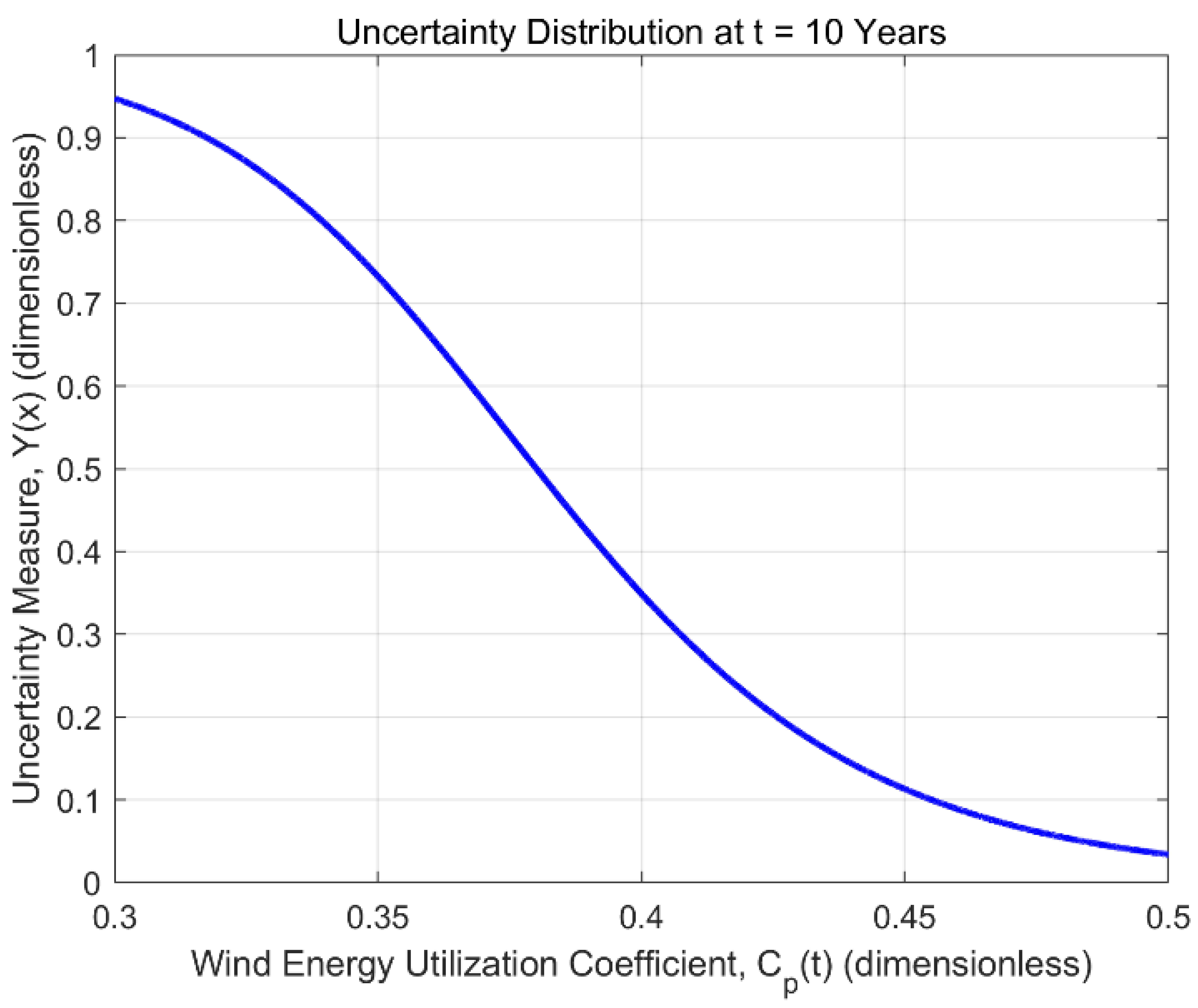
The uncertainty distribution ${\mathsf{\Phi }}_{10}(U_p)$ of the ignition delay time $X_t$ at $t=10\mathrm{years}$ is illustrated in Figure 2. And Figure 3 gives the uncertain measure ${\mathsf{\Phi }}_t(0.38)$, i.e., $\mathcal{M}\left\{U_p^{(t)}\ge 0.38\right\}$.

Uncertainty distribution ${\mathsf{\Phi }}_{10} (U_p)$ of the wind energy utilization coefficient at $t=10$years. The horizontal axis represents possible values of $U_p$; the vertical axis is the uncertainty measure $\mathcal{M}$. The curve shows the epistemic belief that $U_p$ is less than or equal to a given value.

The uncertainty distribution of the wind energy utilization coefficient at a specific time point (e.g., $t=10$ years), as shown in Figure 2, characterizes the epistemic uncertainty in the degradation process. However, for wind farm operators and planners, a more critical concern is how the reliability of meeting a minimum performance requirement evolves over the entire lifecycle. By fixing a threshold value $u_p^{*}$ for the wind energy utilization coefficient—below which the turbine is considered to have unacceptably low efficiency—we can compute the time-dependent belief reliability $R\left(t\right)=\mathcal{M}\left\{U_p\left(t\right)\ge u_p^{*}\right\}$. This metric directly reflects the probability (in the sense of uncertain measure) that the turbine maintains an acceptable performance level at each point in time. As shown in Figure 3, with a threshold of $u_p^{*}=0.38$, the reliability $R\left(t\right)$ decreases monotonically over time. This decreasing trend implies that the probability of the turbine operating with satisfactory efficiency gradually diminishes, and after a certain number of operational years, the reliability falls below an acceptable level. The point in time at which $R\left(t\right)$ crosses a predetermined threshold (e.g., 0.9 or 0.95) defines the reliable life of the turbine with respect to its power generation efficiency. This analysis provides a direct link between the degradation of the physical parameter $U_p^{(t)}$ and the operational reliability of the wind farm’s energy output, offering a quantitative basis for maintenance scheduling and lifecycle management.

Belief reliability $R\left(t\right)=\mathcal{M}\left\{U_p\left(t\right)\ge u_p^{*}\right\}$ over time for a fixed threshold $u_p^{*}=0.38$. This metric quantifies the uncertain measure that the turbine maintains acceptable efficiency. The monotonic decay indicates that after approximately 9 years, the reliability falls below 0.9. A wind farm operator can use this curve to schedule preventive maintenance (e.g., blade cleaning or replacement) once R(t) reaches a predefined threshold, such as 0.85, thereby avoiding unexpected underperformance. A comparative summary of the proposed method against recent wind farm reliability assessment approaches is presented in

Table 3. Comparison of the proposed method with recent approaches for wind farm reliability assessment. Note: ✓ indicates the condition is satisfied; × indicates the condition is not satisfied.

Criterion	Zhang et al. (2023)	Li et al. (2024)	Wang et al. (2025)	This Work
Wake effect modeling	✓ (Jensen)	✓ (CFD)	×	✓ (Jensen)
Performance degradation	×	✓ (linear)	✓ (exponential)	✓ (exponential + Liu)
Aleatory uncertainty	✓ (Weibull)	✓ (normal)	×	✓ (Weibull)
Epistemic uncertainty	×	×	×	✓ (Liu process)
Small-sample capable	× (needs > 50 data)	× (needs > 100 data)	✓ (claims but no validation)	✓ (demonstrated with n = 10)
Unified reliability metric	×	×	✓ (probabilistic)	✓ (belief reliability)

. Compared with existing studies, this work exhibits several distinct advantages: it simultaneously considers wake effects, exponential-Liu performance degradation, Weibull-distributed aleatory uncertainty, and epistemic uncertainty modeled by the Liu process, with validation on a small dataset (n = 10). In addition, the belief reliability metric developed in this paper enables unified quantification of different uncertainty sources, addressing the limitations of traditional methods in small-sample and epistemic uncertainty handling.

6. Discussion and Conclusions

Due to treating wind speed with random uncertainty as a random variable and the degradation of wind energy utilization coefficient with cognitive uncertainty as an uncertain process, the power generation demand margin obtained from the uncertainty calculation of wind speed random variables and wind energy utilization coefficient degradation process is an uncertain random variable, which needs to be measured using an opportunity measure defined in the product space of uncertainty space and probability space.

This study develops a belief reliability modeling method for wind farm energy production by integrating wake effects, performance degradation, and uncertainty analysis, addressing key limitations of existing models. The Jensen wake model, combined with the kinetic energy loss superposition method, effectively quantifies wind speed deficits from single and multiple wake interactions—avoiding the overestimation of energy output that occurs when wake effects are simplified or ignored. The linear degradation model for the wind energy utilization coefficient $U_{\mathrm{p}}$, enhanced with an uncertain Liu process, captures gradual performance decline from factors like blade pollution and control system aging, reducing long-term (10-year) power generation prediction deviations that could otherwise exceed 15%. Additionally, leveraging belief reliability theory overcomes the reliance of traditional probabilistic methods on large failure datasets, enabling accurate reliability assessment even for wind farms with limited historical data by unifying aleatory uncertainty (Weibull-distributed wind speed) and epistemic uncertainty ($U_{\mathrm{p}}$ degradation). Limitations include the Jensen model’s simplification of conical wake diffusion (which may underestimate turbulence impacts in mountainous areas) and the linear $U_{\mathrm{p}}$ degradation assumption (less suitable for extreme conditions like severe corrosion). Overall, this framework improves the accuracy of lifecycle energy production and reliability prediction, providing practical support for wind farm design, maintenance, and energy planning; future work could adopt 3D wake models and non-linear degradation functions to enhance adaptability to complex environments.

The proposed framework supports three key engineering decisions:

(1)

Design optimization. By quantifying how wake losses propagate uncertainty under performance degradation, designers can optimize turbine spacing and layout to balance land use against long-term reliability targets.

(2)

Maintenance scheduling. The reliable life metric $L$ defined in Section 4.4 provides a quantitative trigger for preventive maintenance. For example, if an operator sets $R_{th}=0.9$ and $W_{th}=100 \mathrm{GWh}/\mathrm{year}$, the computed $L\approx 8.5$ years indicates that major maintenance (e.g., blade cleaning or pitch system overhaul) should be scheduled before year 9.

(3)

Energy planning and power purchase agreements (PPAs). The belief reliability $R_{\mathrm{demand}}\left(t\right)$ offers a defensible, data-justified probability (in the uncertain measure sense) that the wind farm will meet contracted energy delivery targets over its lifetime, even when historical failure data are scarce.