CATI: Cross-Attention-Based Task Interaction for Multi-Granular Metro Passenger Flow Forecasting

Abstract

Accurate short-term metro passenger flow forecasting plays a key role in urban transit management, supporting train scheduling, crowd control, and operational planning. Jointly modeling station-level inflow/outflow (IO) and inter-station origin–destination flows (OD/DO) has proven effective for improving prediction accuracy, as it allows the model to leverage dependencies across different flow granularities. However, effectively exploiting such dependencies remains nontrivial. Station-level intensity (IO) and inter-station migration patterns (OD/DO) differ substantially in both representation and dynamics, and the dependencies between them are inherently directional and uneven. As a result, commonly used parameter-sharing mechanisms in multi-task learning are often insufficient to capture informative cross-task interactions. To address this issue, we propose CATI (Cross-Attention-based Task Interaction), a unified framework for joint multi-granular metro flow forecasting. CATI first learns task-specific spatiotemporal representations for IO, OD, and DO flows, and then introduces directed cross-attention with Gated Residual Fusion to model selective and asymmetric interactions across tasks. In addition, an aggregation-consistency regularization is employed to maintain structural coherence between station-level and inter-station predictions. Experiments on real-world metro datasets from Hangzhou and Shanghai show that CATI consistently outperforms strong baselines across multiple prediction horizons and tasks. Further analysis indicates that the model learns adaptive attention patterns, task-dependent gating behaviors, and controlled interaction strengths, which together explain its improved performance. These results suggest that explicitly modeling asymmetric cross-task interactions is important for multi-granular spatiotemporal forecasting in metro systems.

1. Introduction

Urban rail transit has become a core mode of urban mobility due to its high capacity, efficiency, and reliability. However, metro passenger flows exhibit substantial instability and complexity at short time scales, driven by volatile travel demand, peak-hour concentration, operational disturbances, and unexpected events. Accurate short-term passenger flow forecasting is therefore critical for train scheduling, station crowd management, and operational safety, contributing directly to improved efficiency and service quality [1,2]. In this study, metro passenger flow forecasting is formulated as a multi-task regression problem, aiming to predict continuous flow values over future time horizons. Existing studies typically focus on two spatial granularities: station-level inflow and outflow (IO) and inter-station origin-destination flows (OD/DO). Station-level IO forecasting benefits from spatiotemporal graph modeling and sequential learning, which effectively capture local correlations and temporal dependencies [3,4]. In contrast, OD/DO forecasting characterizes directional travel demand between stations, but suffers from high dimensionality, sparsity, and partial observability, leading to unstable multi-step predictions [1,5,6]. This setting requires modeling continuous spatiotemporal demand dynamics rather than assigning discrete labels or categories.

To exploit complementary information across granularities, recent studies adopt multi-task learning paradigms to jointly model IO and OD/DO flows [7,8,9]. Unlike classification-based transportation problems, such as crash severity prediction, which focus on discrete label assignment, multi-granular passenger flow forecasting involves continuous demand estimation over space and time. Most existing approaches rely on shared encoders, mixture-of-experts architectures, or graph-based feature sharing mechanisms, where cross-task interaction is achieved through parameter sharing or symmetric feature fusion [8,9,10]. While effective in more homogeneous settings, these designs are less suitable for multi-granular passenger flow forecasting, where tasks differ substantially in scale, sparsity, and statistical characteristics. In particular, OD and DO flows are sparse and high-dimensional, whereas IO flows are relatively dense and stable. Direct sharing may therefore introduce noise or suppress task-specific patterns. More importantly, the relationships among IO, OD, and DO flows exhibit both structural coupling and directional asymmetry. On the one hand, station-level inflow and outflow correspond to aggregated OD and DO flows, implying that predictions across granularities should remain coherent. On the other hand, OD and DO flows reflect directional movement patterns and path-dependent dynamics, leading to asymmetric dependencies across tasks [9]. In addition, latent representations introduced to mitigate sparsity further weaken direct numerical correspondence across granularities. These properties suggest that cross-task interaction should be selective, directional, and adaptive, rather than uniformly shared.

To address these challenges, we propose CATI (Cross-Attention-based Task Interaction), a multi-granular forecasting framework for joint IO, OD, and DO prediction. CATI adopts an encoder–decoder architecture, where task-specific spatiotemporal representations are first learned independently and then enhanced through directed cross-attention. This design allows each task to selectively incorporate information from other granularities, enabling asymmetric and task-aware information propagation for continuous spatiotemporal regression. In addition, a flow-consistency regularization is introduced to encourage coherence across granularities while preserving task-specific flexibility.

The main contributions of this study are summarized as follows:

(1)

We formulate multi-granular metro passenger flow forecasting as a set of structurally coupled yet heterogeneous regression tasks, characterized by aggregation constraints and directional dependencies, which are not adequately addressed by existing symmetric multi-task learning frameworks.

(2)

We develop CATI, a cross-attention-based interaction framework that enables selective and direction-aware information exchange across IO, OD, and DO flows, providing a flexible alternative to conventional shared-encoder and MMoE-style architectures.

(3)

We introduce a flow-consistency regularization to enhance cross-granular coherence and multi-step stability, and demonstrate the effectiveness of the proposed framework through extensive experiments and ablation studies on real-world metro datasets.

2. Related Work

Short-term metro passenger flow forecasting has been extensively studied from both station-level and inter-station perspectives. Existing work mainly focuses on station-level inflow/outflow (IO) forecasting, inter-station origin–destination/destination–origin (OD/DO) forecasting, and, more recently, their joint modeling via multi-task learning (MTL).

2.1. Station-Level IO Passenger Flow Forecasting

Station-level inflow/outflow (IO) forecasting is one of the most mature research directions in short-term metro passenger flow prediction. Existing studies primarily differ in how they model inter-station spatial correlations and temporal evolution, leading to a gradual progression from topology-driven spatiotemporal modeling toward more adaptive and expressive representations. Early methods predominantly rely on fixed graph structures—such as physical topology, functional similarity, or historical correlations—combined with recurrent or convolutional sequence models to capture spatial dependencies and temporal dynamics. Representative approaches, including PVCGN [11] and MGC-RNN [12], demonstrate strong performance under normal operating conditions, but their dependence on predefined relational priors limits adaptability under peak-demand fluctuations and non-stationary disruptions.

To alleviate the rigidity of static graph assumptions, subsequent studies introduce adaptive and dynamic dependency learning mechanisms that infer latent and time-varying spatial interactions directly from data. Methods such as MR-STN [13], STDGRL [14], PMR-GCN [3], TGCRN [15], ReDyNet [4], and DSTGFN [16] dynamically adjust inter-station interaction patterns to better reflect evolving passenger movement correlations. At the same time, attention mechanisms and Transformer-style architectures have been explored to strengthen temporal dependency modeling, enabling more effective capture of long-range and multi-scale temporal patterns and substantially improving multi-horizon forecasting accuracy [17,18]. Some studies further incorporate higher-order or hierarchical spatial structures, such as STHGARN [19] and hierarchical graph-based approaches [20], to model complex dependencies across multiple levels.

These methods improve the representation of station-level dynamics, but they largely treat IO flows as isolated targets. The interaction between station-level flows and inter-station movements is not explicitly modeled, and the directional propagation of passenger demand across the network is not directly reflected. As a result, IO predictions may become inconsistent with underlying movement patterns, especially under long-horizon forecasting or sudden demand changes.

2.2. Inter-Station OD/DO Passenger Flow Forecasting

Inter-station origin-destination (OD/DO) forecasting provides a fine-grained description of passenger movements between stations and reveals the network-level propagation of travel demand in metro systems. Compared with station-level IO prediction, OD/DO forecasting is inherently more challenging due to the high dimensionality, severe sparsity, and partial observability of OD matrices, especially near the prediction horizon [21,22]. Early studies mainly rely on statistical models or sequence-based approaches, such as matrix decomposition and recurrent neural networks, which are interpretable but limited in capturing spatial structure. Recent work introduces spatiotemporal models that explicitly incorporate graph structures and directional dependencies. Methods such as ST-DAMHGN [1], ODformer [23], PSAM-CNN [5], and ODMixer [6] model cross-station interactions and improve OD prediction performance. Some work also introduces operational constraints into OD prediction. Zhang et al. [24] incorporate section capacity utilization ratios to regularize OD estimates under network capacity limits. However, such approaches mainly constrain OD flows themselves and do not explicitly enforce consistency with station-level IO flows. In addition, to address the delay between trip generation and completion, HIAM [7] jointly models OD and DO flows to reduce temporal misalignment.

Although these methods improve OD/DO prediction, they are typically developed independently of IO modeling. While OD/DO flows inherently encode direction-driven and asymmetric passenger propagation across the network, their predictions are typically optimized without explicit coordination with station-level IO flows. As a result, the conservation relationship between inter-station transfers and station-level marginals is often violated implicitly, especially under multi-step forecasting, where directional errors accumulate over time. This structural mismatch exposes a fundamental challenge in multi-granular passenger flow forecasting: how to jointly model asymmetric OD/DO propagation while preserving conservation-induced consistency across flow granularities, which cannot be adequately addressed by OD/DO-only or loosely coupled modeling paradigms.

2.3. Multi-Task Learning for Joint IO-OD-DO Forecasting

To leverage complementary information across multiple flow granularities, multi-task learning (MTL) has been increasingly adopted in metro passenger flow forecasting. Representative studies such as HIAM [7], Multi-AFFN [8], MTLMetro [9], and recent MMoE-based multi-granular forecasting models jointly predict IO, OD, and DO flows within unified architectures. These methods demonstrate consistent improvements over single-task learning by enabling information sharing, coordinated optimization, and enhanced robustness.

However, existing MTL approaches exhibit several common limitations. First, cross-task interactions are often implemented via shared encoders, feature concatenation, or predefined message-passing channels, resulting in static and coarse-grained information sharing that is insensitive to task-specific relevance or temporal context [9]. Second, most joint frameworks implicitly assume near-symmetric cross-task interactions, which limits their ability to capture direction-driven and asymmetric demand propagation inherent in OD/DO flows. Third, flow conservation is typically treated as an implicit property or a soft regularization term, rather than as an explicit structural constraint [8,9], leaving marginal inconsistencies unresolved under peak loads or disruptions.

In summary, existing work does not explicitly distinguish between directional interaction and conservation constraints in multi-granular passenger flow modeling. This limits the ability of current methods to simultaneously capture demand propagation and maintain structural consistency. To address this issue, we propose CATI, which introduces directed cross-attention to model asymmetric and target-aware interactions while explicitly enforcing conservation consistency across flow granularities.

3. Preliminaries

This section introduces the multi-granular passenger flow representations used, the delayed observability of inter-station OD flows, and the aggregation relations that couple station-level and inter-station flows. These preliminaries clarify the structural dependencies and heterogeneous characteristics of IO, OD, and DO flows, which motivate the cross-task interaction framework proposed in Section 4.

3.1. Definitions

In metro passenger flow forecasting, travel demand can be described at different spatial granularities. Station-level inflow/outflow (IO) captures local entry and exit volumes, while origin-destination (OD) and destination-origin (DO) flows describe directional passenger movements between stations. OD and DO flows explicitly encode directional travel demand from two views. These representations are not independent: they are linked by flow aggregation relations, but also exhibit different statistical properties, dimensional scales, and sparsity patterns. In particular, OD and DO matrices are typically high-dimensional and sparse, while IO flows are relatively dense and stable. Such heterogeneity makes direct parameter sharing across tasks ineffective and motivates the need for adaptive cross-task interaction mechanisms.

Definition 1

(Metro Topological Graph). The metro system is represented as a weighted graph $G=(V,E,W)$, where V denotes the set of N stations, E denotes physical connections between stations, and $W\in {\mathbb{R}}^{N\times N}$ is a weight matrix derived from the row-normalized adjacency of G. The graph structure is assumed to be static across all time slots.

Definition 2

(Station-Level Inflow and Outflow (IO)). The station-level passenger flow at time slot t is denoted as ${\mathit{X}}_t^{IO}\in {\mathbb{R}}^{N\times 2}$. For station i, ${\mathit{X}}_t^{IO}[i,0]$ and ${\mathit{X}}_t^{IO}[i,1]$ represent the inflow (entries) and outflow (exits), respectively. For convenience, we define the inflow and outflow as ${\mathit{X}}_t^I\left[i\right]={\mathit{X}}_t^{IO}[i,0]$ and ${\mathit{X}}_t^O\left[i\right]={\mathit{X}}_t^{IO}[i,1]$.

Definition 3

(Inter-Station OD and DO Flows). The origin-destination (OD) flow at time slot t is defined as ${\mathit{X}}_t^{OD}\in {\mathbb{R}}^{N\times N}$, where ${\mathit{X}}_t^{OD}[i,j]$ denotes the number of passengers entering station i during slot t and heading for destination station j. The destination-origin (DO) flow at time slot t is defined as ${\mathit{X}}_t^{DO}\in {\mathbb{R}}^{N\times N}$, where ${\mathit{X}}_t^{DO}[i,j]$ denotes the number of passengers exiting station i during slot t who previously entered at station j.

Definition 4

(Flow-Conservation Relations). Station-level IO flows and inter-station OD/DO flows are coupled by flow aggregation identities. In particular, they satisfy

$$\sum _j{\mathit{X}}_t^{OD}[i,j]={\mathit{X}}_t^I\left[i\right],and\sum _j{\mathit{X}}_t^{DO}[i,j]={\mathit{X}}_t^O\left[i\right].$$

(1)

These relations indicate that different granular representations correspond to different views of the same passenger movement process and should remain numerically consistent after aggregation. This coupling can be interpreted as a form of structural symmetry across granularities, although the representations are generally heterogeneous and cannot be enforced to be identical.

In practice, OD flows cannot be fully observed in real time because many trips are still in progress within the observation time window. This delayed observability further increases the mismatch between IO and OD/DO representations and makes joint forecasting more challenging.

Definition 5

(Finished and Unfinished Recent OD Flows). Assuming the current time slot is t, the recent OD matrix ${\mathit{X}}_{t-\delta }^{OD}\in {\mathbb{R}}^{N\times N}$ at a near recent time slot $t-\delta$ is partially observable because trip durations vary and there are trips that have not been completed until t, where $0\le \delta <T_h$, and $T_h$ is the looking-back window. Accordingly, the full recent OD flow matrix ${\mathit{X}}_{t-\delta }^{OD}$ at $t-\delta$ can be decomposed into two components: the observed (completed) recent OD ${\mathit{X}}_{t-\delta }^{FOD}\in {\mathbb{R}}^{N\times N}$, and the unobserved (unfinished) recent OD ${\mathit{X}}_{t-\delta }^{UOD}\in {\mathbb{R}}^{N\times N}$, i.e.,

$${\mathit{X}}_{t-\delta }^{OD}={\mathit{X}}_{t-\delta }^{FOD}+{\mathit{X}}_{t-\delta }^{UOD}.$$

(2)

Accordingly, the full recent inflow ${\mathit{X}}_{t-\delta }^I$ can also be divided into two components: finished and unfinished recent inflows, according to trip finished or not until current time slot t.

Definition 6

(Finished and Unfinished Recent Inflows). The finished and unfinished recent inflows at time slot $t-\delta$ are defined as

$${\mathit{X}}_{t-\delta }^{FI}\left[i\right]={\displaystyle \sum _{j=1}^N}{\mathit{X}}_{t-\delta }^{FOD}[i,j],and{\mathit{X}}_{t-\delta }^{UI}\left[i\right]={\displaystyle \sum _{j=1}^N}{\mathit{X}}_{t-\delta }^{UOD}[i,j],i=1,\dots ,N.$$

(3)

In fact, the full recent inflow at $t-\delta$ (Definition 2) satisfies: ${\mathit{X}}_{t-\delta }^I={\mathit{X}}_{t-\delta }^{FI}+{\mathit{X}}_{t-\delta }^{UI}$.

Despite the unfinished recent OD ${\mathit{X}}_{t-\delta }^{UOD}$ is unknown, the unfinished recent inflow ${\mathit{X}}_{t-\delta }^{UI}\left[i\right]$ can be implied from the full recent inflow ${\mathit{X}}_{t-\delta }^I$ and finished recent OD matrix ${\mathit{X}}_{t-\delta }^{FOD}$, i.e., ${\mathit{X}}_{t-\delta }^{UI}\left[i\right]={\mathit{X}}_{t-\delta }^I-{\mathit{X}}_{t-\delta }^{FI}$. To alleviate the delayed observability of recent OD flows and make full advantage of observable flows, we follow HIAM [7] and integrate a recent OD completion module to compensate for the missing features of full recent OD matrices with the unfinished recent inflows, finished recent OD matrices, and periodic regularities of historical OD matrices. In particular, the following two types of periodic regularities are utilized for recent OD information completion.

Definition 7

(Daily Periodic Destination Distribution Matrix). The daily periodic destination distribution matrix ${\mathit{P}}_{t-\delta }^{daily}\in {\mathbb{R}}^{N\times N}$ is estimated from the OD matrix of the same time slot of the previous day, where ${\mathit{P}}_{t-\delta }^{daily}[i,j]$ represents the probability that a passenger entering station i during slot $t-\delta$ travels to destination station j.

Definition 8

(Weekly Periodic Destination Distribution Matrix). The weekly periodic destination distribution matrix ${\mathit{P}}_{t-\delta }^{weekly}\in {\mathbb{R}}^{N\times N}$ is estimated from OD matrices of the same time slots of the same weekdays in the past few weeks, where ${\mathit{P}}_{t-\delta }^{weekly}[i,j]$ represents the probability that a passenger entering station i during slot $t-\delta$ travels to destination station j.

3.2. Problem Formulation

Let t denote the current time slot. Given a historical window of length $T_h$ and a forecasting horizon of length $T_f$, the goal of this work is to jointly predict station-level IO flows and inter-station OD/DO flows over the next $T_f$ slots. Unlike conventional single-task forecasting, the joint prediction of IO, OD, and DO involves multiple heterogeneous tasks with different dimensionality, sparsity, and statistical characteristics. In addition, these tasks are structurally coupled through aggregation relations, which require the predicted flows to remain mutually consistent after aggregation. Therefore, the key challenge is to design a forecasting framework that enables effective information interaction across granularities while preserving cross-granular coherence.

The joint forecasting problem is defined as learning a parameterized predictor $\mathrm{F}(·;\Theta )$ by solving

$$\begin{array}{cc}\hfill \underset{\Theta }{min}& \mathcal{L}\left(\widehat{\mathcal{Y}},\mathcal{Y}\right), \hfill \end{array}$$

(4)

$$\begin{array}{cc}\hfill \mathrm{s}.\mathrm{t}.& \widehat{\mathcal{Y}}=\mathrm{F}\left(\mathcal{X},G;\Theta \right), \hfill \end{array}$$

(5)

$$\begin{array}{cc}\hfill & \widehat{\mathcal{Y}}=\left({\widehat{\mathit{Y}}}_{t+1:t+T_f}^{IO},{\widehat{\mathit{Y}}}_{t+1:t+T_f}^{OD},{\widehat{\mathit{Y}}}_{t+1:t+T_f}^{DO}\right),\hfill \end{array}$$

(6)

$$\begin{array}{cc}\hfill & \mathcal{Y}=\left({\mathit{Y}}_{t+1:t+T_f}^{IO},{\mathit{Y}}_{t+1:t+T_f}^{OD},{\mathit{Y}}_{t+1:t+T_f}^{DO}\right), \hfill \end{array}$$

(7)

$$\begin{array}{cc}\hfill & \mathcal{X}=\left({\mathit{X}}_{t-T_h+1:t}^{IO},{\mathit{X}}_{t-T_h+1:t}^{FOD},{\mathit{X}}_{t-T_h+1:t}^{UI},{\mathit{X}}_{t-T_h+1:t}^{DO}\right).\hfill \end{array}$$

(8)

Here, ${\mathit{X}}_{\tau }^{IO}\in {\mathbb{R}}^{N\times 2}$ and ${\mathit{X}}_{\tau }^{OD},{\mathit{X}}_{\tau }^{DO}\in {\mathbb{R}}^{N\times N}$ (Definitions 2 and 3); ${\mathit{X}}_{\tau }^{FOD}$ and ${\mathit{X}}_{\tau }^{UI}$ explicitly account for the delayed observability of recent OD flows (Definition 5). For each recent slot $\tau \in [t-T_h+1,t]$, an imputed OD input ${\widehat{\mathit{X}}}_{\tau }^{OD}$ is estimated from $\left({\mathit{X}}_{\tau }^{FOD},{\mathit{X}}_{\tau }^{UI}\right)$, and is used as the OD sequence fed to the model. The metro topology graph G is defined in Definition 1, and $\mathcal{E}$ collects optional exogenous features aligned with time slots.

The learning objective $\mathcal{L}(·)$ consists of task-specific forecasting losses for IO/OD/DO and a consistency regularization term derived from the aggregation relations (Definition 4), which encourages cross-granular coherence while allowing task-specific and direction-dependent dynamics.

4. Methodology

We propose CATI (Cross-Attention-based Task Interaction), a multi-task spatiotemporal forecasting framework for jointly modeling OD, DO, and IO flows. The model follows a structured design that separates task-specific representation learning from cross-task information propagation. Each task is first encoded independently using a task-specific spatiotemporal backbone, and is then refined through cross-task interaction based on cross-attention. A gated residual mechanism is further introduced to regulate the strength of information transfer and reduce the impact of noisy signals.

4.1. Overall Architecture

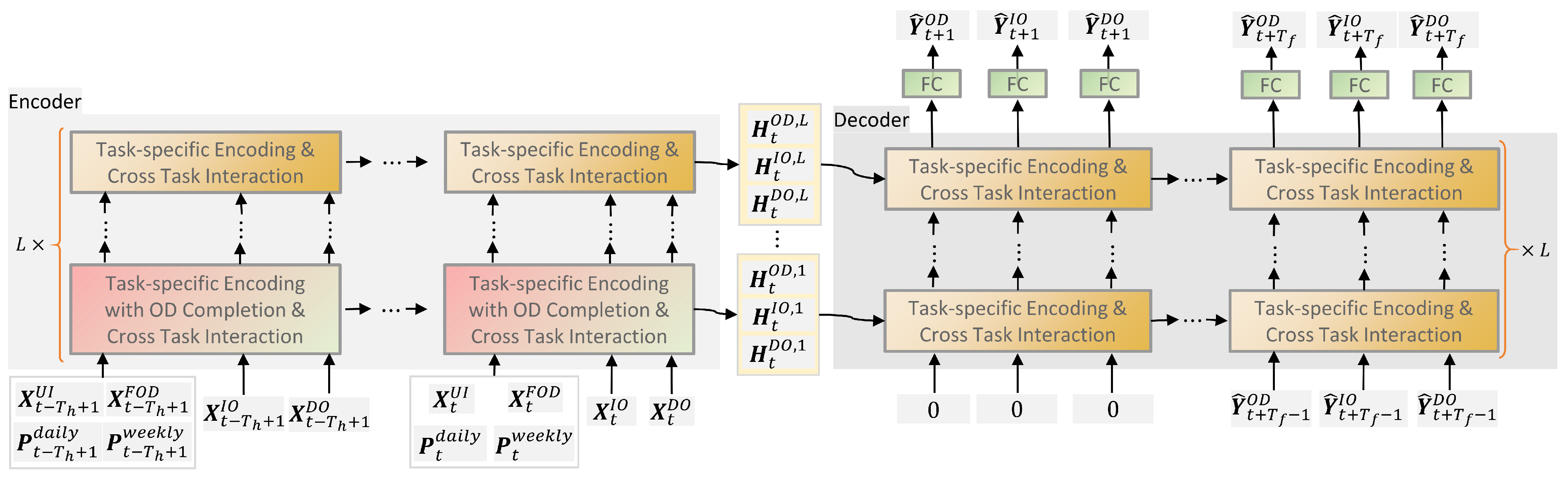
As illustrated in Figure 1, CATI adopts an encoder–decoder architecture for multi-step forecasting. Both the encoder and decoder are composed of L stacked Task-specific Encoding and Cross-Task Interaction (TECTI) modules. Each TECTI module consists of two components: (1) Task-specific encoding block, which models temporal dynamics and spatial correlations within each task independently, producing stable and semantically consistent representations; and (2) cross-task interaction block, which enables directed information exchange across IO, OD, and DO representations, allowing each task to selectively incorporate complementary signals from others.

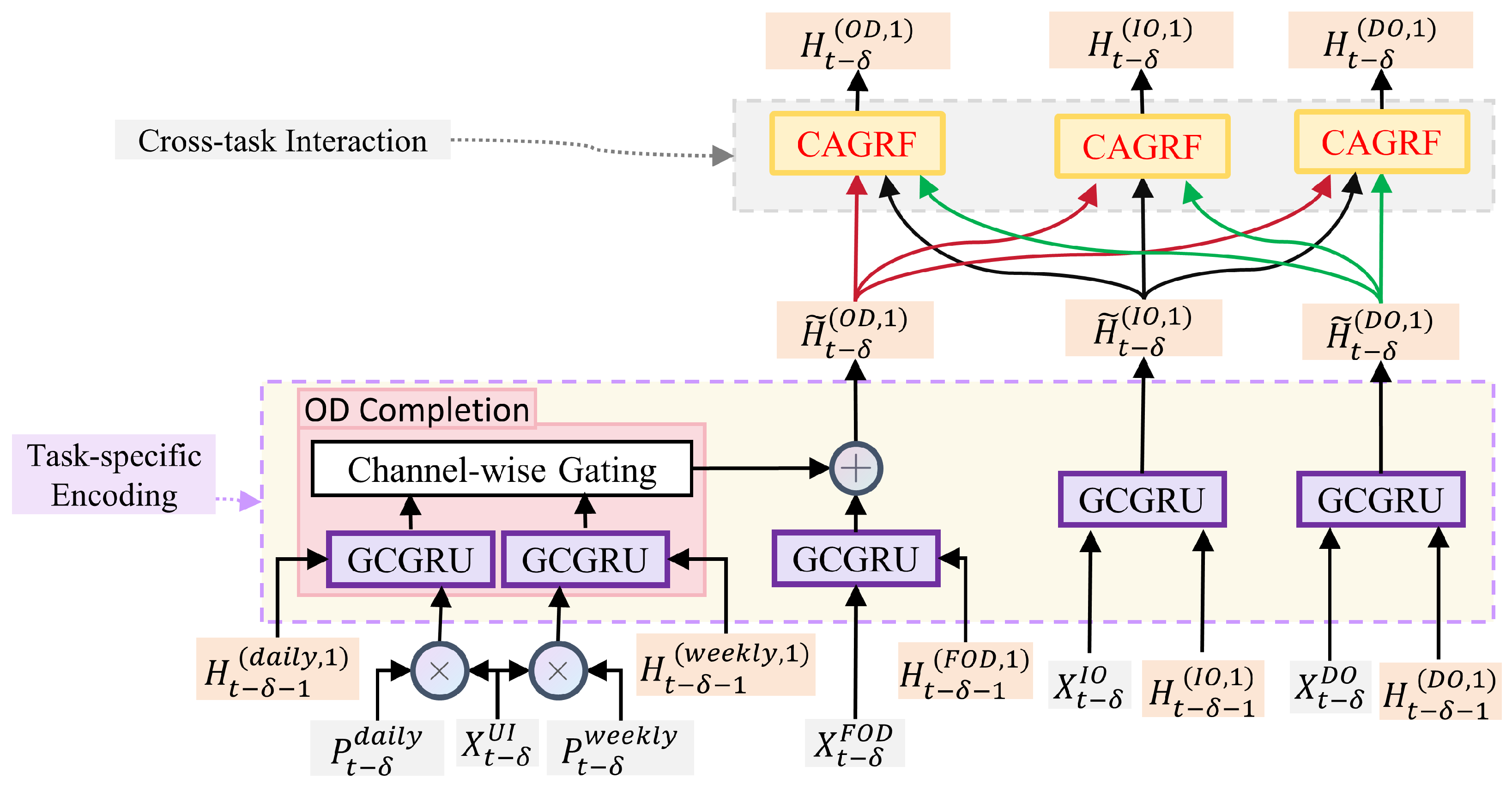
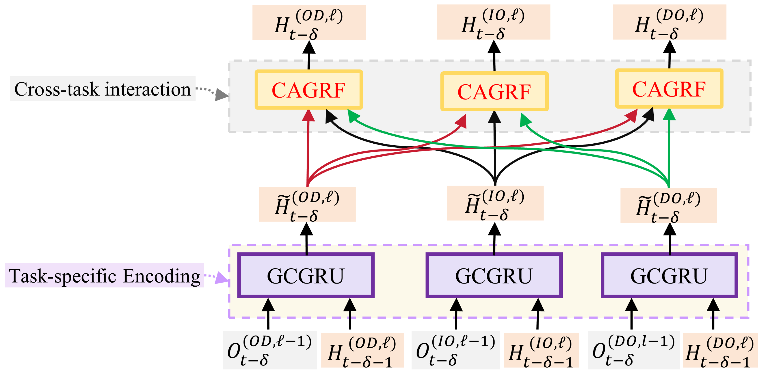
To better handle the sparsity and partial observability of OD/DO flows, we introduce two variants of the TECTI module. The first variant incorporates an OD completion (ODC) mechanism (see Figure 2) which is applied only in the first encoder layer to provide an initial enhancement of OD/DO representations. All subsequent encoder layers and the entire decoder use the standard TECTI module without ODC (see Figure 3) focusing on iterative refinement through cross-task interaction. Stacking multiple TECTI modules allows the encoder to progressively aggregate historical spatiotemporal information, while the decoder generates future predictions in an auto-regressive manner conditioned on the encoded states. This design enables joint multi-granular forecasting within a unified framework, while maintaining a clear separation between within-task modeling, cross-task interaction, and aggregation-level consistency.

To provide a clearer description of the model, we next detail each component of CATI. We begin with the task-specific encoding module (Section 4.2), which learns spatiotemporal representations for each flow granularity independently. We then introduce the cross-task interaction module (Section 4.3), named the Cross-Attention and Gated Residual Fusion (CAGRF) module (see Figure 4), which enables selective and directed information exchange across tasks. Based on these components, we describe the decoder with cross-task interaction for multi-step forecasting in Section 4.4. Finally, the training objective and optimization procedure are presented in Section 4.5.

4.2. Task-Specific Encoding

Within each TECTI module, CATI first independently encodes IO, OD, and DO flows using a task-specific encoding block. This step ensures stable, semantically coherent spatiotemporal representations before any cross-task interaction. OD and DO flows are high-dimensional and sparse with partial observability, whereas IO flows are dense and temporally smooth. Directly sharing parameters or fusing features prematurely may introduce noise or suppress task-specific patterns. In particular, the classical Graph Convolutional Gated Recurrent Unit (GCGRU) [11] is leveraged for task-specific encoding.

4.2.1. GCGRU

GCGRU [11] extends the standard GRU by replacing node-wise affine transformations with graph convolutions, thereby enabling joint modeling of temporal dynamics and non-Euclidean spatial dependencies. Given the input feature $X_t\in {\mathbb{R}}^{N\times C_{\mathrm{in}}}$ and previous hidden state $H_{t-1}\in {\mathbb{R}}^{N\times D_{\mathrm{GCGRU}}}$, the GCGRU update equations are

$$\begin{array}{c}{r}_t=\sigma \left({\Theta }_r{★}_G[X_t,H_{t-1}]+b_r\right),\end{array}$$

(9)

$$\begin{array}{c}{u}_t=\sigma \left({\Theta }_u{★}_G[X_t,H_{t-1}]+b_u\right),\end{array}$$

(10)

$$\begin{array}{c}{c}_t=tanh\left({\Theta }_c{★}_G[X_t,(r_t\odot H_{t-1})]+b_c\right),\end{array}$$

(11)

$$\begin{array}{c}{H}_t=u_t\odot H_{t-1}+(1-u_t)\odot c_t,\end{array}$$

(12)

where ${★}_G$ denotes a GCN-style graph convolution applied over the metro topology graph G (Definition 1), $[·,·]$ denotes feature-wise concatenation, and ⊙ is the Hadamard product, and $D_{\mathrm{GCGRU}}$ is the dimension of the hidden state. For brevity, we simply denote the whole GCGRU computation as

$$H_t=\mathrm{GCGRU}(X_t,H_{t-1};G),$$

(13)

where G is the same topology shared across all time steps. When ${★}_G$ degenerates to a dense linear transformation, GCGRU reduces to a standard GRU.

4.2.2. OD Flow Encoding

Due to real-time aggregation latency, inter-station OD observations are partially available. To mitigate this issue, the first encoder layer ($\ell =1$) of OD encoder incorporates a representation-level OD completion mechanism, inspired by the historical-guided strategy in HIAM [7].

At layer ℓ and time $t-\delta$ ($1\le \ell \le L$ and $0\le \delta <T_h$), the pre-interaction hidden state of OD flow is updated as

$${\tilde{\mathit{H}}}_{t-\delta }^{(OD,\ell )}=\left\{\begin{array}{cc}\mathrm{GCGRU}\left({\mathit{X}}_{t-\delta }^{FOD},\mathbf{0};G\right)+{\mathit{H}}_{t-\delta }^{(UOD,1)},& \mathrm{for}\ell =1,\\ \mathrm{GCGRU}\left({\mathit{H}}_{t-\delta }^{(OD,\ell -1)},{\mathit{H}}_{t-\delta -1}^{(OD,\ell )};G\right),& \mathrm{for}\ell >1.\end{array}\right.$$

(14)

Here, ${\mathit{H}}_{t-\delta }^{(UOD,1)}$ is a compensation term generated from the OD completion module with the short-term (previous day) and long-term (previous weeks) historical OD statistics through channel-wise gated fusion. Specifically, the completion is formulated as follows:

$$\begin{array}{cc}\hfill {\mathit{H}}_{t-\delta }^{(UOD,1)}& ={\alpha }_{t-\delta }\odot {\mathit{H}}_{t-\delta }^{(weekly,1)}+{\beta }_{t-\delta }\odot {\mathit{H}}_{t-\delta }^{(daily,1)}, \hfill \end{array}$$

(15)

$$\begin{array}{cc}\hfill {\mathit{H}}_{t-\delta }^{(daily,1)}& =\mathrm{GCGRU}\left({\mathit{X}}_{t-\delta }^{UI}\times {\mathit{P}}_{t-\delta }^{daily},\mathbf{0},G\right), \hfill \end{array}$$

(16)

$$\begin{array}{cc}\hfill {\mathit{H}}_{t-\delta }^{(weekly,1)}& =\mathrm{GCGRU}\left({\mathit{X}}_{t-\delta }^{UI}\times {\mathit{P}}_{t-\delta }^{weekly},\mathbf{0},G\right), \hfill \end{array}$$

(17)

$$\begin{array}{cc}\hfill {\mathit{\alpha }}_{t-\delta }& =\sigma \left({\mathit{W}}_{\alpha }\left[{\mathit{H}}_{t-\delta }^{(weekly,1)};{\mathit{H}}_{t-\delta }^{(daily,1)}\right]+{\mathit{b}}_{\alpha }\right),\hfill \end{array}$$

(18)

$$\begin{array}{cc}\hfill {\mathit{\beta }}_{t-\delta }& =\sigma \left({\mathit{W}}_{\beta }\left[{\mathit{H}}_{t-\delta }^{(weekly,1)};{\mathit{H}}_{t-\delta }^{(daily,1)}\right]+{\mathit{b}}_{\beta }\right),\hfill \end{array}$$

(19)

where ${\mathit{P}}_{t-\delta }^{daily},{\mathit{P}}_{t-\delta }^{weekly}\in {\mathbb{R}}^{N\times N}$ are daily and weekly periodic destination distribution matrices; see Definitions 7 and 8, separately. This residual formulation preserves observed OD structure while compensating for missing inter-station dependencies. In addition, the completion procedure is applied only in the first encoder layer. ${\mathit{H}}_{t-\delta }^{(OD,\ell -1)}$ is the output hidden states of the previous layer, which includes the augmentation residual item resulting from other tasks with the cross-task interaction layer.

4.2.3. DO and IO Flow Encoding

IO and DO flows are directly encoded via GCGRUs, separately. At layer ℓ and time $t-\delta$ ($1\le \ell \le L$ and $0\le \delta <T_h$), the pre-interaction hidden state of $z\in \{\mathrm{IO},\mathrm{DO}\}$ is updated as

$${\tilde{\mathit{H}}}_{t-\delta }^{(z,\ell )}=\left\{\begin{array}{cc}\mathrm{GCGRU}\left({\mathit{X}}_{t-\delta }^z,\mathbf{0};G\right),& \mathrm{for}\ell =1,\\ \mathrm{GCGRU}\left({\mathit{H}}_{t-\delta }^{(z,\ell -1)},{\mathit{H}}_{t-\delta -1}^{(z,\ell )};G\right),& \mathrm{for}\ell >1.\end{array}\right.$$

(20)

The same graph G is shared across tasks to ensure consistent spatial modeling, while parameters are kept task-specific to capture heterogeneous dynamics.

The separation between task-specific encoding and cross-task interaction is critical because different granularities exhibit heterogeneous characteristics: OD and DO flows are high-dimensional and sparse, whereas IO flows are dense and relatively stable. Direct parameter sharing or symmetric fusion across tasks may introduce noise or suppress task-specific patterns. CATI mitigates this by first learning task-specific representations and then performing adaptive, direction-aware cross-task interaction. The aggregation relations between IO, OD, and DO flows imply that predictions across granularities should remain consistent after aggregation. Instead of enforcing these relations during representation learning, CATI incorporates them as an aggregation-consistency regularization during training (Section 4.5.1), which improves cross-granular coherence while preserving the flexibility of task-specific modeling.

4.3. Cross-Task Interaction

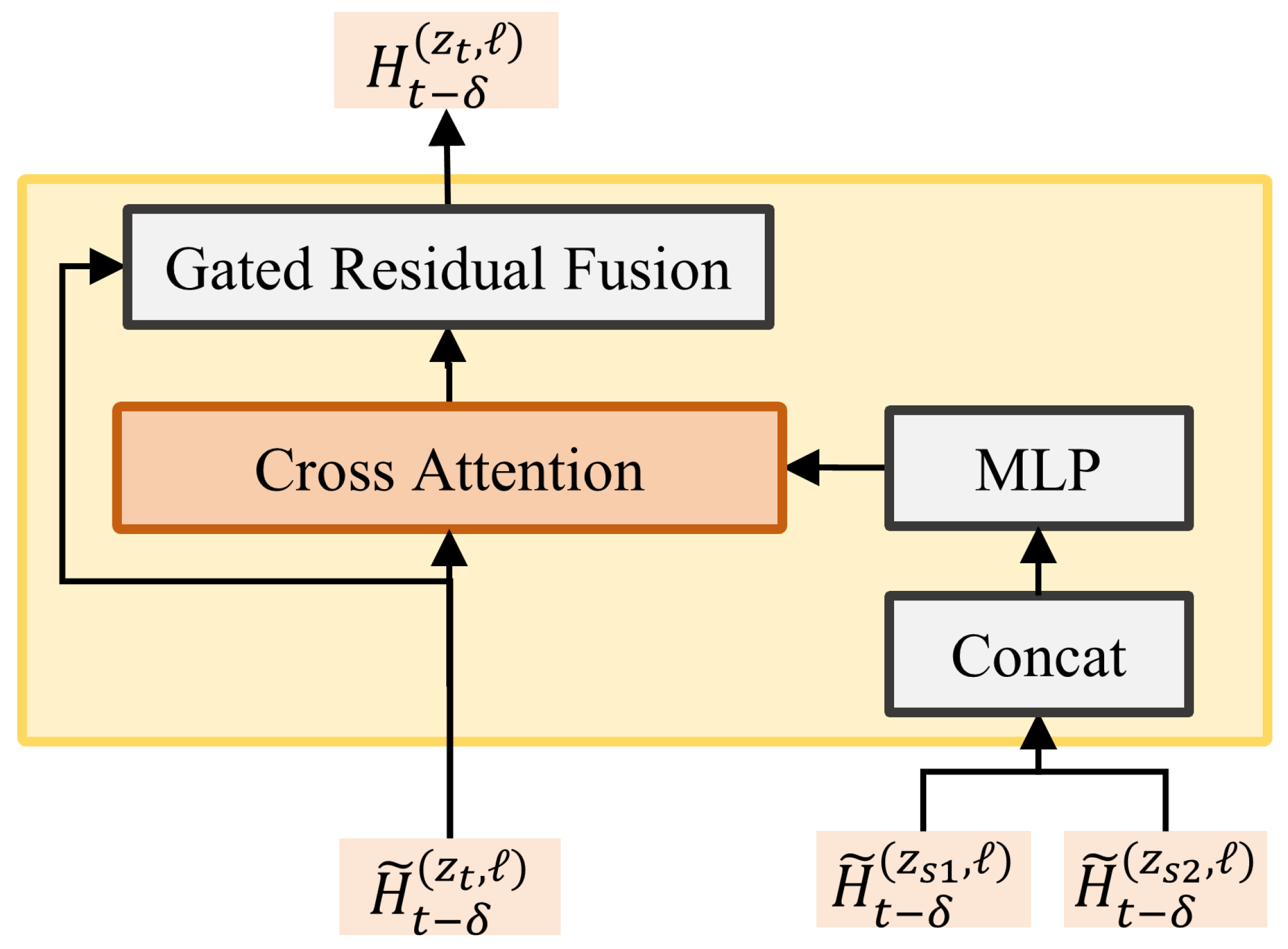
The task-specific spatiotemporal representations introduced in Section 4.2 capture intra-task dynamics but do not explicitly model dependencies across tasks. In multi-granular passenger-flow forecasting, IO, OD, and DO flows are intrinsically coupled through aggregation relations, while exhibiting heterogeneous statistical properties such as sparsity, dimensionality, and directional semantics. Therefore, effective cross-task interaction should enable each task to selectively leverage complementary information from other tasks, without disrupting its own representation space. To this end, we design a pre-fusion Cross-Attention with Gated Residual Fusion interaction mechanism, named CAGRF (see Figure 4), which performs unified multi-source aggregation followed by target-conditioned information selection and Gated Residual Fusion. This design corresponds to an interaction paradigm under a fixed routing topology, where each task receives information from the other two tasks.

4.3.1. Cross-Attention

Cross-attention [25] is adopted as an implementation of the directed task-interaction operator, which propagates information from a source task $z_s$ to a target task $z_t$. Let $H_{f,t}^{(z_t,\ell )}\in {\mathbb{R}}^{N\times D_{\mathrm{GCGRU}}}$ and $H_{f,t}^{(z_s,\ell )}\in {\mathbb{R}}^{N\times D_{\mathrm{GCGRU}}}$ denote the task-specific hidden representations at layer ℓ produced by the task-specific encoder (Section 4.2), where $z_t\ne z_s$ and $z_t,z_s\in \{\mathrm{IO},\mathrm{OD},\mathrm{DO}\}$. The cross-attention computation is defined as

$$\begin{array}{cc}\hfill Q^{\left(z_t\right)}=W_Q^{\left(z_t\right)}{H}_{f,t}^{(z_t,\ell )},K^{\left(z_s\right)}& =W_K^{\left(z_s\right)}{H}_{f,t}^{(z_s,\ell )},V^{\left(z_s\right)}=W_V^{\left(z_s\right)}{H}_{f,t}^{(z_s,\ell )},\hfill \end{array}$$

(21)

$$\begin{array}{cc}\hfill {\widehat{H}}_{f,t}^{z_s\to z_t}& =\mathrm{Softmax}\left({\displaystyle \frac{Q^{\left(z_t\right)}{\left(K^{\left(z_s\right)}\right)}^{\top }}{\sqrt{d}}}\right)V^{\left(z_s\right)},\hfill \end{array}$$

(22)

where $W_Q^{\left(z_t\right)}\in {\mathbb{R}}^{D_{\mathrm{GCGRU}}\times D_{\mathrm{CA}}}$, $W_K^{\left(z_t\right)}\in {\mathbb{R}}^{D_{\mathrm{GCGRU}}\times D_{\mathrm{CA}}}$, $W_V^{\left(z_t\right)}\in {\mathbb{R}}^{D_{\mathrm{GCGRU}}\times D_{\mathrm{CA}}}$ are parameters to be learned, $D_{\mathrm{CA}}$ is the dimension of hidden state of cross-attention, and $\mathrm{Softmax}(·)$ is applied row-wise. For convenience, we simply denote the procedure as

$${\widehat{H}}_{f,t}^{z_s\to z_t}=\mathrm{CrossAtt}\left(H_{f,t}^{(z_t,\ell )},H_{f,t}^{(z_s,\ell )}\right).$$

(23)

This operator is inherently order-sensitive, i.e., $\mathrm{CrossAtt}(H^{\left(z_t\right)},H^{\left(z_s\right)})\ne \mathrm{CrossAtt}(H^{\left(z_s\right)},H^{\left(z_t\right)})$, which naturally supports the direction-driven asymmetric interactions. When $z_t=z_s$, the operator reduces to self-attention.

In CATI, the $\mathrm{CrossAtt}(·)$ operator serves as a basic interaction primitive. The final interaction output for each task is obtained through multi-source aggregation and residual injection, while cross-granular coherence is further enforced by the conservation-consistency regularization.

4.3.2. Pre-Fusion Cross-Task Interaction

Let ${\tilde{\mathit{H}}}_{t-\delta }^{(z,\ell )}$ denote the pre-interaction representation of task $z\in \{\mathrm{IO},\mathrm{OD},\mathrm{DO}\}$ at layer ℓ and time $t-\delta$. For a target task $z_t$, we first aggregate all source task representations $\{{\tilde{\mathit{H}}}_{t-\delta }^{(z_s,\ell )}:z_s\in \mathcal{S}\left(z_t\right)\}$ into a unified embedding via a learnable fusion function:

$${\mathit{H}}_{t-\delta }^{(S,\ell )}=\mathrm{MLP}\left(\mathrm{Concat}{\left[{\tilde{\mathit{H}}}_{t-\delta }^{(z_s,\ell )}\right]}_{z_s\in \mathcal{S}\left(z_t\right)}\right),$$

(24)

where $\mathrm{MLP}(·)$ is a Multi-Layer Perceptron module. Under the interaction setting, $\mathcal{S}\left(z_t\right)=\{\mathrm{IO},\mathrm{OD},\mathrm{DO}\}\setminus \left\{z_t\right\}$. Based on the fused representation, cross-task interaction is computed using cross-attention:

$${\widehat{\mathit{H}}}_{t-\delta }^{(z_t,\ell )}=\mathrm{CrossAttn}\left({\tilde{\mathit{H}}}_{t-\delta }^{(z_t,\ell )},{\mathit{H}}_{t-\delta }^{(S,\ell )}\right),$$

(25)

where $\mathrm{CrossAttn}(·)$ is defined in Section 4.3.1. In Equation (25), the target-task representation serves as the query, while the fused multi-task representation provides keys and values. This design allows the model to perform target-conditioned selection over multi-source information, rather than treating each source independently. Compared with independent pairwise interactions, pre-fusion enforces early alignment across tasks, enabling the model to capture globally consistent cross-granular patterns.

4.3.3. Gated Residual Integration

To integrate cross-task information into the target representation, we adopt a gated residual update:

$${\mathit{G}}_{t-\delta }^{(z_t,\ell )}=\sigma \left({\mathit{W}}_g\left[{\tilde{\mathit{H}}}_{t-\delta }^{(z_t,\ell )};{\widehat{\mathit{H}}}_{t-\delta }^{(z_t,\ell )}\right]+{\mathit{b}}_g\right),$$

(26)

$${\mathit{H}}_{t-\delta }^{(z_t,\ell )}={\tilde{\mathit{H}}}_{t-\delta }^{(z_t,\ell )}+{\mathit{G}}_{t-\delta }^{(z_t,\ell )}\odot \varphi \left({\widehat{\mathit{H}}}_{t-\delta }^{(z_t,\ell )}\right),$$

(27)

where $\sigma (·)$ denotes the sigmoid function, $\varphi (·)$ is a non-linear transformation (using $tanh(·)$ in CATI), and ${\mathit{G}}_{t-\delta }^{(z_t,\ell )}$ controls the contribution of cross-task information. This mechanism plays a critical role in stabilizing multi-task learning. It preserves task-specific semantics while allowing adaptive information injection, effectively mitigating negative transfer caused by noisy or conflicting cross-task signals.

The proposed interaction mechanism is characterized by three key properties: (1) Pre-fusion interaction. Multi-source information is first aligned in a shared latent space before interaction, which reduces conflicts across heterogeneous tasks. (2) Target-conditioned selection. Cross-attention ensures that each task selectively extracts relevant information based on its current representation. (3) Gated residual injection. Adaptive gating controls the strength of cross-task information, improving robustness and preventing negative transfer. Together, these properties enable effective and stable cross-task information propagation in multi-granular passenger-flow forecasting.

4.4. Decoder with Cross-Task Interaction

Based on the interaction-enhanced representations learned by the encoder, the decoder generates future predictions in an auto-regressive manner. At each prediction step, the decoder maintains task-specific hidden states and continues to incorporate cross-task information through the same interaction mechanism. Specifically, for each task $z\in \{\mathrm{IO},\mathrm{OD},\mathrm{DO}\}$ at the ℓ layer and $t+k$ time slot ($1\le \ell \le L$ and $1\le k\le T_f$), the decoder updates its hidden state as:

$${\tilde{\mathit{H}}}_{t+k}^{(z,\ell )}=\left\{\begin{array}{cc}\mathrm{GCGRU}\left({\mathit{X}}_{t+k-1}^z,{\mathit{H}}_{t+k-1}^{(z,\ell )};G\right),& \mathrm{for}\ell =1,\\ \mathrm{GCGRU}\left({\mathit{H}}_{t+k}^{(z,\ell -1)},{\mathit{H}}_{t+k-1}^{(z,\ell )};G\right),& \mathrm{for}\ell >1.\end{array}\right.$$

(28)

where ${\mathit{X}}_{t+k-1}^z$ is the input at time $t+k-1$, which is either the ground truth or the model prediction from the previous step. After each layer, cross-task interaction is applied:

$${\mathit{H}}_{t+k}^{(z,\ell )}=\mathrm{CAGRF}\left({\tilde{\mathit{H}}}_{t+k}^{(IO,\ell )},{\tilde{\mathit{H}}}_{t+k}^{(OD,\ell )},{\tilde{\mathit{H}}}_{t+k}^{(DO,\ell )}\right),$$

(29)

where $\mathrm{CAGRF}(·)$ follows the pre-fusion Cross-Attention with Gated Residual Fusion interaction mechanism defined in Section 4.3, and $1\le k\le T_f$. This design ensures that cross-task dependencies are consistently modeled during both encoding and decoding, allowing the model to dynamically refine predictions based on evolving task representations.

Finally, the prediction for each task is obtained via a linear projection:

$${\widehat{\mathit{Y}}}_{t+k}^z=\mathrm{FC}\left({\mathit{H}}_{t+k}^{(z,L)}\right)={\mathit{W}}_o^{\left(z\right)}{\mathit{H}}_{t+k}^{(z,L)},z\in \{\mathrm{OD},\mathrm{DO},\mathrm{IO}\}.$$

(30)

To mitigate exposure bias in multi-step forecasting, we adopt a curriculum learning strategy that gradually transitions from teacher forcing to fully autoregressive decoding.

4.5. Training Objective and Algorithm

CATI is trained to jointly predict OD, DO, and IO flows over multiple horizons. The training alternates between forward propagation through the encoder–decoder and backpropagation of gradients with respect to a combined loss.

4.5.1. Training Objective

To jointly optimize multi-granular passenger-flow prediction while preserving structural consistency across tasks, we adopt a structure-aware multi-task objective that decouples representation learning from aggregation constraints. Specifically, the overall objective consists of two components: (1) task-specific prediction losses, which supervise each task independently, and (2) an aggregation-consistency regularization, which enforces coherence across different granularities at the output level.

The overall loss is defined as:

$$\mathcal{L}=\sum _{z\in \{\mathrm{OD},\mathrm{DO},\mathrm{IO}\}}{\lambda }_z{\mathcal{L}}_z+{\lambda }_{\mathrm{con}}{\mathcal{L}}_{\mathrm{con}},$$

(31)

where ${\lambda }_z$ and ${\lambda }_{\mathrm{con}}$ balance task accuracy and cross-task consistency. In our implementation, these weights are fixed during training and selected based on validation experiments. Keeping the regularization weight constant avoids degenerating to single-task optimization and ensures that cross-granular consistency is preserved throughout the forecasting horizon.

Task-Specific Prediction Losses

For each task, we adopt mean absolute error (MAE) over the prediction horizon $T_f$:

$${\mathcal{L}}_z=\mathrm{MAE}\left({\widehat{\mathit{Y}}}_{t+1:t+T_f}^z,{\mathit{Y}}_{t+1:t+T_f}^z\right),z\in \{\mathrm{OD},\mathrm{DO},\mathrm{IO}\}.$$

(32)

These losses directly supervise each task branch, allowing the model to learn task-specific dynamics without interference from other tasks. This design is consistent with the representation-level decoupling introduced in Section 4.2, where each task maintains its own feature space before cross-task interaction.

Aggregation-Consistency Regularization

Although task representations are learned independently, IO, OD, and DO flows are inherently coupled through aggregation relations. To enforce this structural dependency, we introduce a consistency regularization that aligns predicted station-level flows with those implied by inter-station flows. Specifically, we compute an implied IO flow from predicted OD and DO:

$${\tilde{\mathit{Y}}}_{t+1:t+T_f}^{\mathrm{IO}}=\mathrm{Aggregate}\left({\widehat{\mathit{Y}}}_{t+1:t+T_f}^{\mathrm{OD}},{\widehat{\mathit{Y}}}_{t+1:t+T_f}^{\mathrm{DO}}\right),$$

(33)

where $\mathrm{Aggregate}(·)$ denotes the aggregation operator defined by flow conservation.

The consistency loss is then defined as:

$${\mathcal{L}}_{\mathrm{con}}=\mathrm{MAE}\left({\widehat{\mathit{Y}}}_{t+1:t+T_f}^{\mathrm{IO}},{\tilde{\mathit{Y}}}_{t+1:t+T_f}^{\mathrm{IO}}\right).$$

(34)

Unlike task-specific losses, ${\mathcal{L}}_{\mathrm{con}}$ does not introduce additional supervision, but instead acts as a structural regularizer that enforces cross-granular consistency at the prediction level.

The above objective reflects a key design principle of our framework: task representations are learned independently, while their predictions are coupled through structural constraints. This decoupling is critical for multi-granular forecasting. Enforcing aggregation relations directly in the representation space may overly constrain feature learning and degrade task-specific performance. Instead, by imposing consistency only at the output level, the model retains sufficient flexibility in representation learning while ensuring coherent predictions across granularities. The proposed objective complements the cross-task interaction mechanism in Section 4.3. While cross-attention enables adaptive information sharing at the representation level, the consistency regularization enforces global coherence at the output level. Together, they provide a balanced framework for multi-task learning under heterogeneous data distributions.

4.5.2. Training Algorithm

The overall training procedure of CATI is summarized in Algorithm 1. The model is trained end-to-end under the encoder–decoder architecture described in Section 4.1, where task-specific encoding and cross-task interaction are applied sequentially at each layer. Given historical IO, OD, and DO sequences, the encoder produces interaction-enhanced representations, which are then used by the decoder for multi-step prediction in an auto-regressive manner. The composite loss defined in Section 4.5.1 is optimized using the Adam optimizer. To improve stability for long-horizon forecasting, we adopt an inverse-sigmoid curriculum learning strategy, which gradually transitions from teacher forcing to fully auto-regressive decoding. The learning rate is initialized to $0.001$ and scheduled using MultiStepLR, and early stopping is applied based on validation performance. All hyperparameters are selected on the validation set and fixed across all experiments.

4.5.3. Computational Complexity

For a single layer, the GCGRU module consists of graph message passing and gated transformations, with a time complexity of $O\left(\left|E\right|·D_{GCGRU}+N·D_{GCGRU}^2\right)$, where N is the number of stations, $\left|E\right|$ is the number of edges, and $D_{GCGRU}$ is the hidden-state dimension. The cross-task interaction in CATI adopts a pre-fusion strategy. Specifically, multi-source features are first fused via a linear projection, yielding a complexity of $O\left(N·M·D_{GCGRU}^2\right)$, where M denotes the number of auxiliary sources (a small constant in the three-task setting). The subsequent cross-attention includes query/key/value projections, attention score computation, aggregation, and output projection, leading to a complexity of

$$O\left(N^2·D_{CA}+N·D_{GCGRU}·D_{CA}+N·D_{CA}^2\right),$$

where $D_{CA}$ is the attention channel dimension. Since interaction is performed for all tasks, the overall complexity of the interaction module remains in the same order. Combining all components, the per-layer, per-time-step complexity is

$$O\left(\left|E\right|·D_{GCGRU}+N·D_{GCGRU}^2+N^2·D_{CA}+N·D_{GCGRU}·D_{CA}+N·D_{CA}^2\right).$$

Considering all epochs, samples, sequence length T, and stacked layers L, the total training complexity is

$$O\left(N_{epochs}·N_S·T·L·\left(\left|E\right|·D_{GCGRU}+N·D_{GCGRU}^2+N^2·D_{CA}+N·D_{GCGRU}·D_{CA}+N·D_{CA}^2\right)\right).$$

In practice, since $D_{CA}=O\left(D_{GCGRU}\right)$ and $\left|E\right|\le N^2$, this can be simplified as

$$O\left(N_{epochs}·N_S·T·L·\left(N·D_{GCGRU}^2+N^2·D_{GCGRU}\right)\right),$$

where the $O(N·D_{GCGRU}^2+N^2·D_{GCGRU})$ term typically dominates.

Algorithm 1: Training algorithm of CATI

5. Experiments

5.1. Experimental Setup

To comprehensively evaluate the performance of the proposed model, experiments are conducted on two real-world metro passenger flow datasets. This section introduces the experimental setup, including dataset descriptions, evaluation metrics, baseline models, and implementation details.

5.1.1. Datasets

We evaluate the proposed model on two real-world metro passenger flow datasets collected from Shanghai (SHMetro) and Hangzhou (HZMetro), originally released in PVCGN [11] and HIAM [7]. These datasets are derived from real metro operation systems and contain synchronized station-level inflow/outflow (IO) and inter-station OD and DO flows, enabling multi-granular passenger-flow forecasting.

Table 1. The datasets used in the experiments.

Name	SHMetro	HZMetro
City	Shanghai	Hangzhou
Number of stations	288	80
Number of physical edge	958	248
Averaged ridership per day	8.82 M	2.35 M
Time interval	15 min	15 min
Working time each day	5:30–23:30	5:30–23:30
Training timespan	1 July–31 August 2016	1–18 January 2019
Number of training samples	4092	1188
Validation timespan	1–9 September 2016	19–20 January 2019
Number of validation samples	594	132
Testing timespan	10–30 September 2016	21–25 January 2019
Number of testing samples	1386	330

summarizes the main statistics of the two datasets, including the number of stations, network size, time span, and number of samples. The SHMetro dataset spans from 1 July 2016 to 30 September 2016, covering 288 stations with an average daily ridership of approximately 8.82 million passengers. The HZMetro dataset covers January 2019, including 80 stations with an average daily ridership of 2.35 million. In both datasets, metro services operate between 5:30 and 23:30, and passenger flows are aggregated at 15 min intervals. For each time slot, the data include station-level inflow and outflow volumes, as well as OD and DO matrices describing passenger movements between stations. The OD and DO matrices exhibit strong sparsity, with most entries being zero at each time slot. In addition, passenger flow distributions are highly skewed, where a small number of stations and OD pairs account for the majority of trips. This long-tailed distribution introduces inherent data imbalance and makes multi-granular forecasting particularly challenging.

Data variables and preprocessing. The input features consist of metro network topology information and historical IO, OD, and DO flow observations. All features are numerical, and no additional temporal or categorical variables are introduced. The datasets are pre-cleaned and contain no missing values. It is worth mentioning that the OD and DO data released in HIAM [7] are already represented in a compressed form, where each matrix is reduced from $N\times N$ to $N\times N^{\prime }$. This compression is part of the original dataset release rather than a preprocessing step performed in this work. Specifically, the top $N^{\prime }-1$ destinations with the largest flows are retained, while the remaining stations are aggregated into a single column. We set $N^{\prime }=76$ for SHMetro and $N^{\prime }=26$ for HZMetro. All experiments in this study are conducted on this released compressed representation. The compression strategy introduces a trade-off between computational efficiency and spatial detail preservation. By reducing the dimensionality of OD/DO matrices, the model becomes more scalable and easier to train, especially for large metro networks. However, aggregating low-flow station pairs into a single column may lead to a loss of fine-grained spatial information. In practice, this trade-off is mitigated by retaining the most significant destinations with the largest flows, which preserves the dominant mobility patterns while discarding less informative interactions. This strategy has been shown to be effective in prior work such as HIAM [7], and we follow the same setting to ensure a fair and consistent comparison. Prior to training, all input features are normalized using Z-score normalization to stabilize optimization. During inference, model outputs are transformed back to the original scale, and all loss functions and evaluation metrics are computed in the original data space. No additional feature engineering or feature selection techniques are applied.

To reflect real-world forecasting scenarios and avoid information leakage, both datasets are divided chronologically into training, validation, and testing sets. The split ratios are approximately 70%, 10%, and 20%, with slight variations across datasets (see Table 1). All models are trained and evaluated on the same splits.

5.1.2. Evaluation Metrics

Since passenger-flow forecasting is a regression task, the performance of all models is evaluated using three widely adopted error metrics in spatiotemporal forecasting: Mean Absolute Error (MAE), Root Mean Square Error (RMSE), and Mean Absolute Percentage Error (MAPE). These metrics measure prediction accuracy from complementary perspectives, including absolute deviation, squared deviation, and relative error magnitude. Formally, for a forecasting horizon of length $T_f$, the metrics are defined as

$$\begin{array}{cc}\hfill MAE& ={\displaystyle \frac{1}{T_f}}{\displaystyle \sum _{i=1}^{T_f}}\left|{\mathit{Y}}_i-{\widehat{\mathit{Y}}}_i\right|,\hfill \end{array}$$

(35)

$$\begin{array}{cc}\hfill RMSE& =\sqrt{{\displaystyle \frac{1}{T_f}}\sum _{i=1}^{T_f}{\left({\mathit{Y}}_i-{\widehat{\mathit{Y}}}_i\right)}^2},\hfill \end{array}$$

(36)

$$\begin{array}{cc}\hfill MAPE& ={\displaystyle \frac{1}{T_f}}{\displaystyle \sum _{i=1}^{T_f}}\left|{\displaystyle \frac{{\mathit{Y}}_i-{\widehat{\mathit{Y}}}_i}{{\mathit{Y}}_i}}\right|.\hfill \end{array}$$

(37)

Here, ${\mathit{Y}}_i$ and ${\widehat{\mathit{Y}}}_i$ denote the ground-truth and predicted passenger flows at the i-th future time step, respectively. These metrics are computed for each forecasting horizon and then averaged over all test samples.

Because this study focuses on continuous passenger-flow prediction rather than classification, accuracy-based metrics such as precision or recall are not applicable. Instead, MAE, RMSE, and MAPE are widely used in traffic flow forecasting and spatiotemporal prediction, and allow fair comparison with existing methods. In addition to prediction accuracy, we also evaluate the consistency between station-level and inter-station predictions. Following the aggregation relations defined in Section 3, we compute the discrepancy between predicted IO flows and the IO flows implied by OD/DO predictions, which reflects the degree of cross-granular inconsistency. This metric is reported in the ablation study to analyze the effect of the conservation-consistency regularization.

It is worth noting that different evaluation metrics exhibit varying sensitivity to flow magnitudes. MAE and RMSE are more influenced by large-flow stations and peak periods, while MAPE is relatively more sensitive to low-flow conditions due to its normalization by ground truth values. As a result, these metrics provide complementary perspectives for evaluating model performance across different demand levels. In metro systems, passenger flows typically exhibit strong temporal heterogeneity, with pronounced peak and off-peak patterns. Although this work focuses on overall performance, the proposed model is designed to handle both high-demand and low-demand scenarios through adaptive cross-task interaction. A more fine-grained analysis of error distribution across different demand regimes (e.g., peak vs. non-peak periods) is left for future work.

5.1.3. Baselines

To evaluate the effectiveness of CATI, we compare it with a diverse set of representative baselines covering sequence-based, graph-based, Transformer-based, and metro-specific forecasting models. These baselines span different modeling paradigms for temporal dependencies, spatial correlations, and multi-task passenger-flow prediction, providing a comprehensive benchmark. All models are trained under the same data splits, training protocols, and evaluation metrics to ensure a fair comparison. For models originally designed for single-task prediction, output layers are adapted to match the IO–OD–DO forecasting setting without altering their core architecture.

• LSTM: Vanilla LSTM stacked two hidden layers with 256 units each and ReLU activation, only capturing temporal dependencies.
• GRU: Vanilla GRU stacked two hidden layers with hidden dimension 256, only capturing temporal dependencies.
• GCN: Learns spatial correlations via graph convolutions, followed by a fully connected layer to predict flows.
• Diffusion Convolutional RNN (DCRNN) [26]: Integrates diffusion convolutions with recurrent layers to jointly model spatial and temporal dependencies.
• Graph WaveNet (GWN) [27]: Combines adaptive spatial dependencies with stacked dilated causal convolutions for long-term temporal modeling.
• Discrete Graph Structure Learning (DGSL) [28]: Learns an optimized graph topology to capture temporal-spatial dependencies dynamically.
• PVCGN [11]: Designed for metro systems, incorporating multi-graph modeling and GC-GRU for spatiotemporal dependency learning.
• MGT [17]: Transformer-based model with spatiotemporal self-attention and meta-learned parameters for heterogeneous station characteristics.
• Informer [29]: Sparse attention Transformer for long-sequence forecasting, adapted for IO prediction.
• STAEformer [30]: Introduces spatiotemporal adaptive embeddings into Transformer frameworks, enabling graph-free modeling.
• ReDyNet [4]: Focused on station-level IO prediction, learning dynamic graphs and filtering redundant context via information bottleneck.
• HIAM [7]: Jointly predicts OD/DO flows using a dual-information Transformer; IO predictions are obtained by aggregating OD/DO outputs.

Sequence models (LSTM, GRU) capture temporal dependencies but ignore spatial structure. Graph-based models (GCN, DCRNN, GWN, DGSL, PVCGN) jointly model spatial topology and temporal dynamics. Transformer-based methods (Informer, MGT, STAEformer) emphasize long-range dependencies and adaptive representation learning. ReDyNet focuses on station-level IO, whereas HIAM models OD/DO with derived IO. In contrast, CATI explicitly models direction-aware cross-task interactions among IO, OD, and DO flows in a unified framework, enabling structured information exchange without imposing hard constraints. Only reproducible baselines with publicly available implementations are included, ensuring comparability under the same experimental protocol. Other recent multi-task forecasting models (e.g., AFFN [8], MTLMetro [9]) are excluded due to unavailable code or incompatible task definitions.

5.1.4. Implementation Details

All models are trained under a rolling forecasting setting, where the past four time intervals ($T_h=4$) are used to predict the next four intervals ($T_f=4$). All flow data are standardized using Z-score normalization before training to improve numerical stability. During inference, model outputs are transformed back to the original scale, and all loss functions and evaluation metrics are computed in the original data space. Model parameters are initialized using Xavier uniform initialization and optimized with the Adam optimizer. The initial learning rate is set to 0.002, and a learning rate decay strategy is applied when the validation loss does not improve for 20 consecutive epochs, with decay ratios of 0.2 for SHMetro and 0.5 for HZMetro. The maximum number of training epochs is 200, and the batch size is set to 16 for SHMetro and 32 for HZMetro. Early stopping based on validation performance is adopted to prevent overfitting.

To ensure fair comparison, all models are trained under the same experimental protocol, including identical data splits, input length, forecasting horizon, input features, and evaluation metrics. Hyperparameters such as learning rate, hidden dimension, and number of layers are selected based on commonly used settings in prior work and further tuned on the validation set, and the same training procedure is applied to all baselines. To improve reproducibility and reduce the influence of random initialization, each experiment is repeated five times with different random seeds, and the reported results correspond to the average performance, with standard deviations reported where necessary. All experiments are implemented in PyTorch 2.1.0 and conducted on a Linux server equipped with an NVIDIA GeForce RTX 4090 GPU (24 GB VRAM), manufactured by NVIDIA Corporation (Santa Clara, California, USA). For the proposed CATI model, the number of stacked layers is set to $L=2$, the hidden dimension of GCGRU modules is $D_{\mathrm{GCGRU}}=96$, the hidden dimension of cross-attention modules is $D_{\mathrm{CA}}=512$, and the head of cross-attention modules is $N_h=4$. PReLU is used as the activation function.

5.2. Overall Forecasting Performance

The overall comparison results on HZMetro and SHMetro datasets against the baselines are reported in

Table 2. Comparison of prediction performance with baseline models on HZMetro dataset. The results of CATI are reported as mean ± standard deviation over five runs with different random seeds. Bold values indicate the best results.

Metric	Task	Time	GRU	LSTM	GCN	DCRNN	GWN	DGSL	PVCGN	STAE-Former	ReDy-Net	HIAM	CATI ± std
MAPE (%)	OD	15 min	31.58	30.48	32.12	31.20	32.96	31.45	29.89	29.66	28.40	27.86	27.49 ± 0.13
		30 min	31.04	30.49	32.31	31.28	33.64	31.81	30.53	29.51	28.63	27.90	27.55 ± 0.11
		45 min	30.59	30.34	32.76	31.54	35.53	32.50	30.78	29.64	28.90	28.04	27.72 ± 0.12
		60 min	30.57	30.61	33.38	31.81	36.72	33.35	31.05	30.17	29.41	28.22	27.93 ± 0.14
	DO	15 min	32.28	31.96	32.69	30.81	33.78	31.69	30.02	29.83	29.24	28.61	28.31 ± 0.07
		30 min	32.37	31.58	33.32	30.93	33.45	31.99	30.51	30.06	29.21	28.63	28.35 ± 0.05
		45 min	32.58	31.61	34.40	31.37	33.57	32.65	31.02	30.43	29.14	28.85	28.57 ± 0.04
		60 min	32.40	31.55	35.61	32.01	34.31	33.59	31.48	31.08	29.69	29.16	28.84 ± 0.05
	IO	15 min	15.92	15.14	15.40	10.58	14.48	10.24	9.73	9.83	9.67	10.27	9.22 ± 0.08
		30 min	15.28	14.31	15.19	10.97	14.66	10.34	10.13	10.01	10.04	10.63	9.55 ± 0.07
		45 min	14.66	14.13	15.86	11.53	15.47	10.69	10.49	10.37	10.23	11.00	9.96 ± 0.06
		60 min	14.47	14.04	16.04	11.97	15.59	11.10	10.73	10.55	10.33	11.35	10.30 ± 0.05
MAE	OD	15 min	2.73	2.63	2.78	2.70	2.85	2.74	2.69	2.66	2.63	2.50	2.47 ± 0.01
		30 min	2.65	2.60	2.76	2.67	2.87	2.77	2.74	2.64	2.65	2.50	2.47 ± 0.01
		45 min	2.57	2.55	2.75	2.65	2.99	2.81	2.75	2.64	2.66	2.50	2.47 ± 0.01
		60 min	2.54	2.54	2.77	2.64	3.05	2.85	2.75	2.66	2.68	2.50	2.47 ± 0.01
	DO	15 min	2.81	2.79	2.83	2.69	2.95	2.76	2.68	2.69	2.61	2.56	2.53 ± 0.01
		30 min	2.82	2.75	2.84	2.69	2.91	2.78	2.74	2.69	2.65	2.57	2.55 ± 0.00
		45 min	2.82	2.73	2.89	2.71	2.90	2.82	2.79	2.73	2.73	2.59	2.57 ± 0.00
		60 min	2.77	2.70	2.95	2.74	2.94	2.88	2.83	2.79	2.71	2.62	2.59 ± 0.00
	IO	15 min	35.92	34.17	34.76	23.88	32.69	23.11	22.66	22.64	22.52	23.93	21.49 ± 0.20
		30 min	34.22	32.06	34.02	24.58	32.84	23.16	23.65	22.98	22.82	24.80	22.30 ± 0.16
		45 min	32.49	31.32	35.15	25.55	34.28	23.70	24.65	23.60	23.53	25.64	23.20 ± 0.14
		60 min	31.71	30.77	35.15	26.24	34.17	24.32	24.86	24.34	24.23	26.30	23.86 ± 0.11
RMSE	OD	15 min	5.94	5.77	5.78	5.55	6.34	5.14	5.38	5.23	5.18	4.90	4.63 ± 0.06
		30 min	5.72	5.70	5.85	5.59	6.57	5.40	5.78	5.23	5.19	4.93	4.70 ± 0.05
		45 min	5.58	5.68	6.04	5.73	7.20	5.62	5.91	5.24	5.22	4.98	4.75 ± 0.06
		60 min	5.73	5.84	6.16	5.70	7.63	5.77	6.01	5.85	5.56	5.02	4.80 ± 0.05
	DO	15 min	6.47	6.23	5.98	5.17	6.47	5.25	5.27	5.23	5.21	4.88	4.82 ± 0.01
		30 min	6.68	6.09	6.26	5.22	6.25	5.41	5.63	5.47	5.36	4.96	4.90 ± 0.01
		45 min	6.88	6.03	6.67	5.31	6.08	5.66	5.89	5.51	5.42	5.06	5.00 ± 0.02
		60 min	6.65	5.95	6.99	5.41	6.12	5.99	5.99	5.52	4.48	5.16	5.10 ± 0.03
	IO	15 min	72.40	62.46	58.45	39.90	54.79	38.75	38.06	37.52	37.39	38.88	35.74 ± 0.72
		30 min	68.57	58.42	57.76	41.78	54.52	38.64	40.06	38.49	37.46	40.31	37.15 ± 0.56
		45 min	64.14	57.05	60.89	42.84	58.40	39.70	41.63	39.37	38.54	41.72	38.78 ± 0.58
		60 min	60.42	56.51	59.48	43.92	56.79	40.71	42.21	40.06	39.89	43.30	40.19 ± 0.48

and

Table 3. Comparison of prediction performance with baseline models on SHMetro dataset. The results of CATI are reported as mean ± standard deviation over five runs with different random seeds. Bold values indicate the best results.

Metric	Task	Time	GRU	LSTM	GCN	DCRNN	GWN	DGSL	PVCGN	STAE-Former	ReDy-Net	HIAM	CATI ± std
MAPE (%)	OD	15 min	45.80	45.43	42.30	40.78	41.67	40.84	39.32	38.96	38.69	38.11	37.54 ± 0.04
		30 min	47.31	47.03	42.56	40.63	41.35	40.93	39.44	39.10	39.03	38.06	37.47 ± 0.05
		45 min	49.28	49.00	43.52	40.92	41.32	41.49	39.67	39.25	39.12	38.26	37.66 ± 0.08
		60 min	51.40	51.07	44.93	41.67	42.55	42.40	40.15	39.44	39.26	38.60	37.95 ± 0.10
	DO	15 min	42.13	41.86	42.43	40.58	42.21	40.66	39.30	39.22	39.06	38.95	38.31 ± 0.03
		30 min	43.22	42.86	42.68	40.65	42.04	40.71	39.60	39.61	39.23	38.85	38.25 ± 0.03
		45 min	45.22	44.77	43.64	41.17	42.09	41.24	40.24	40.21	39.92	39.09	38.50 ± 0.04
		60 min	47.35	46.76	45.01	41.19	42.15	42.14	41.06	40.79	40.27	39.49	38.87 ± 0.07
	IO	15 min	19.68	18.65	19.34	11.98	14.92	10.59	10.44	10.35	10.25	14.70	9.91 ± 0.06
		30 min	18.42	17.81	19.28	12.74	14.66	10.90	10.97	11.07	10.86	14.82	10.32 ± 0.07
		45 min	17.91	17.73	19.76	13.86	15.02	11.57	11.48	11.22	11.09	15.06	10.74 ± 0.08
		60 min	17.67	17.80	19.74	14.89	15.32	12.16	12.03	11.40	11.33	15.29	11.09 ± 0.09
MAE	OD	15 min	1.33	1.32	1.23	1.18	1.20	1.18	1.14	1.13	1.13	1.10	1.09 ± 0.00
		30 min	1.36	1.35	1.24	1.16	1.18	1.19	1.13	1.12	1.12	1.09	1.08 ± 0.00
		45 min	1.40	1.39	1.26	1.16	1.17	1.20	1.13	1.12	1.12	1.09	1.07 ± 0.00
		60 min	1.44	1.43	1.29	1.16	1.19	1.22	1.13	1.12	1.12	1.08	1.06 ± 0.00
	DO	15 min	1.22	1.21	1.23	1.18	1.22	1.18	1.14	1.13	1.13	1.13	1.11 ± 0.00
		30 min	1.26	1.25	1.24	1.18	1.22	1.18	1.15	1.14	1.14	1.13	1.11 ± 0.00
		45 min	1.31	1.30	1.26	1.19	1.22	1.20	1.17	1.16	1.15	1.14	1.12 ± 0.00
		60 min	1.37	1.35	1.30	1.21	1.21	1.21	1.19	1.18	1.17	1.14	1.12 ± 0.00
	IO	15 min	42.95	40.70	43.65	26.33	32.55	23.12	23.92	22.63	22.48	32.40	21.84 ± 0.12
		30 min	40.02	38.41	43.19	27.93	31.86	23.69	24.96	23.33	23.17	32.59	22.70 ± 0.15
		45 min	38.62	38.23	43.79	30.18	32.38	24.95	25.87	23.99	23.95	32.91	23.47 ± 0.17
		60 min	37.67	37.95	43.26	32.09	32.66	25.92	26.73	24.77	24.94	33.09	23.99 ± 0.21
RMSE	OD	15 min	4.12	4.07	3.29	3.22	3.47	2.96	3.17	2.94	2.89	2.82	2.71 ± 0.01
		30 min	4.60	4.55	3.37	3.31	3.36	3.04	3.32	2.99	2.93	2.89	2.79 ± 0.01
		45 min	5.12	5.08	3.58	3.48	3.36	3.19	3.42	3.07	3.02	2.96	2.86 ± 0.03
		60 min	5.59	5.59	3.86	3.67	3.70	3.38	3.62	3.21	3.11	3.02	2.93 ± 0.04
	DO	15 min	3.22	3.17	3.34	2.98	3.49	2.97	2.92	2.90	2.89	2.86	2.71 ± 0.01
		30 min	3.53	3.48	3.42	3.05	3.45	3.05	3.02	2.95	2.91	2.89	2.77 ± 0.01
		45 min	4.06	4.07	3.62	3.18	3.44	3.18	3.22	3.08	3.01	2.96	2.84 ± 0.01
		60 min	4.60	4.70	3.84	3.34	3.42	3.39	3.59	3.21	3.12	3.04	2.91 ± 0.01
	IO	15 min	95.88	87.68	72.85	50.49	64.38	44.50	47.89	43.75	42.97	51.64	42.01 ± 0.37
		30 min	88.68	84.01	71.85	54.63	63.19	47.50	51.94	46.33	45.46	52.92	44.81 ± 0.54
		45 min	85.35	84.25	73.45	61.14	65.37	52.13	55.31	48.45	47.78	54.88	47.56 ± 0.68
		60 min	83.47	84.03	71.93	66.36	65.24	55.74	59.92	50.34	50.01	56.75	49.87 ± 0.91

, separately. From the results, we can observe that CATI achieves the best performance across all tasks and horizons. To further evaluate robustness, we report the results of CATI as mean ± standard deviation over five runs with different random seeds. The standard deviations are consistently small across all tasks and forecasting horizons, indicating that the performance improvements are stable and not sensitive to random initialization. Sequence models capture temporal dependencies but lack spatial coupling. Graph-based models leverage topological propagation but do not explicitly align station-level intensity (IO) with inter-station migration (OD/DO), leading to uneven gains across tasks. HIAM improves OD/DO via task interaction, but IO relies on simple aggregation and exhibits instability for long horizons. CATI explicitly models directed cross-task dependencies via layer-wise cross-attention, allowing progressive alignment between OD/DO migration and IO intensity. Coupled with conservation-consistency regularization, the model stabilizes predictions and mitigates task-specific overfitting, delivering consistent improvements across datasets and horizons.

The relative performance of baselines aligns with their modeling biases. Pure sequence models (GRU, LSTM) capture temporal dependencies but under-represent spatial coupling. Graph-based spatiotemporal models (GCN, DCRNN, GWN, DGSL, PVCGN) strengthen topological propagation, yet they lack explicit mechanisms to align station-level and inter-station representations, which can lead to uneven gains across tasks. HIAM improves OD/DO by enhancing OD-DO interaction, but its IO is obtained via aggregation without dedicated task supervision, limiting long-horizon stability. In contrast, CATI explicitly models directed cross-task dependencies via layer-wise cross-attention, enabling progressive alignment between migration structure (OD/DO) and station-level intensity (IO) at multiple depths. Together with the conservation-consistency regularizer, CATI mitigates task-wise overfitting and stabilizes cross-granular predictions, thereby delivering balanced and reproducible improvements across both datasets and all horizons.

5.3. Ablation Study

To evaluate the effectiveness of the proposed CATI model components, we conduct a comprehensive ablation study from two perspectives: (i) analysis of the cross-task interaction mechanisms and (ii) evaluation of aggregation-consistency regularization. All experiments are conducted on HZMetro and SHMetro datasets, and results are reported using standard metrics (MAPE, MAE, RMSE) across different prediction horizons.

5.3.1. Impact of Cross-Task Interaction Mechanisms

We first assess the contribution of cross-task interactions by comparing the following six model variants:

• Ind+Cons: independent task modeling with consistency regularization but without any cross-task interaction.
• woGate: full cross-task interaction but without the gated residual mechanism.
• EncOnly: cross-task interaction applied only in the encoder layers.
• DecOnly: cross-task interaction applied only in the decoder layers.
• PosFusion: post-fusion strategy replacing our proposed pre-fusion design.
• Full (CATI): the complete model with pre-fusion, gated residuals, and encoder–decoder cross-task interaction.

As shown in

Table 4. Ablation study on cross-task interaction mechanisms on HZMetro and SHMetro datasets. Bold values indicate the best results.

			HZMetro						SHMetro
Metric	Task	Time	Ind+Cons	woGate	EncOnly	DecOnly	PosFusion	Full	Ind+Cons	woGate	EncOnly	DecOnly	PosFusion	Full
MAPE (%)	OD	15 min	32.43	27.39	28.65	27.70	28.34	27.41	39.16	37.52	38.16	37.95	38.46	37.53
		30 min	34.04	27.47	28.77	27.72	28.37	27.49	39.17	37.41	38.02	37.89	38.39	37.50
		45 min	36.60	27.59	29.19	27.88	28.68	27.68	39.55	37.53	38.26	38.03	38.58	37.69
		60 min	39.36	27.80	29.89	28.13	29.09	27.81	40.13	37.78	38.71	38.27	38.91	37.97
	DO	15 min	34.35	28.22	28.94	28.28	28.74	28.32	41.47	38.31	38.98	38.93	39.08	38.32
		30 min	36.65	28.29	28.92	28.27	28.64	28.36	41.99	38.24	38.95	38.82	39.05	38.26
		45 min	40.43	28.48	29.27	28.47	28.92	28.55	43.00	38.48	39.29	38.99	39.34	38.49
		60 min	45.08	28.72	29.94	28.69	29.39	28.83	44.12	38.86	39.69	39.22	39.75	38.85
	IO	15 min	14.09	9.35	10.17	9.23	9.51	9.10	11.55	10.13	10.11	9.87	10.15	9.86
		30 min	18.06	9.63	10.70	9.47	9.90	9.38	12.56	10.41	10.49	10.28	10.56	10.27
		45 min	23.01	9.95	11.23	9.86	10.41	9.76	13.72	10.78	10.91	10.73	11.02	10.68
		60 min	27.93	10.28	11.65	10.22	10.87	10.06	14.89	11.09	11.22	11.09	11.43	11.00
MAE	OD	15 min	2.91	2.46	2.58	2.49	2.55	2.46	1.13	1.09	1.11	1.10	1.11	1.09
		30 min	3.05	2.46	2.58	2.49	2.55	2.47	1.13	1.08	1.09	1.09	1.10	1.08
		45 min	3.27	2.46	2.61	2.49	2.56	2.47	1.13	1.07	1.09	1.08	1.10	1.07
		60 min	3.48	2.46	2.64	2.49	2.57	2.46	1.12	1.06	1.08	1.07	1.09	1.06
	DO	15 min	3.07	2.52	2.59	2.53	2.57	2.53	1.20	1.11	1.13	1.13	1.13	1.11
		30 min	3.29	2.54	2.60	2.54	2.57	2.55	1.22	1.11	1.13	1.13	1.14	1.11
		45 min	3.64	2.56	2.63	2.56	2.60	2.57	1.25	1.12	1.14	1.13	1.14	1.12
		60 min	4.05	2.58	2.69	2.58	2.64	2.59	1.28	1.12	1.15	1.13	1.15	1.12
	IO	15 min	32.83	21.78	23.70	21.51	22.16	21.21	25.45	22.32	22.29	21.75	22.37	21.74
		30 min	42.15	22.47	24.98	22.10	23.10	21.89	27.63	22.90	23.07	22.62	23.22	22.60
		45 min	53.62	23.18	26.15	22.97	24.25	22.74	29.98	23.57	23.84	23.46	24.09	23.34
		60 min	64.74	23.83	27.00	23.68	25.19	23.33	32.22	24.00	24.28	23.99	24.72	23.80
RMSE	OD	15 min	6.10	4.72	5.04	4.69	4.93	4.59	2.90	2.75	2.76	2.74	2.78	2.69
		30 min	6.57	4.75	5.14	4.72	4.96	4.66	2.98	2.78	2.85	2.83	2.86	2.78
		45 min	7.47	4.80	5.25	4.77	5.06	4.73	3.11	2.84	2.92	2.92	2.93	2.85
		60 min	8.43	4.87	5.40	4.82	5.14	4.75	3.20	2.88	2.95	2.99	3.00	2.92
	DO	15 min	6.99	4.78	4.98	4.77	4.92	4.81	3.02	2.73	2.77	2.70	2.76	2.71
		30 min	7.69	4.85	5.07	4.83	4.95	4.89	3.22	2.77	2.84	2.76	2.82	2.77
		45 min	9.10	4.95	5.16	4.94	5.07	4.97	3.51	2.84	2.97	2.85	2.92	2.84
		60 min	10.99	5.03	5.30	5.04	5.22	5.06	3.90	2.90	3.04	2.92	2.99	2.89
	IO	15 min	62.93	36.85	41.02	35.66	37.87	35.06	48.62	43.64	42.14	41.22	42.48	42.04
		30 min	80.92	37.76	43.60	36.54	39.44	36.44	55.52	45.47	44.52	44.26	45.32	44.64
		45 min	104.29	38.99	45.62	38.19	41.58	38.00	63.15	47.97	47.38	47.53	48.16	47.20
		60 min	127.75	40.62	47.55	39.60	43.72	39.20	72.68	49.97	49.18	50.15	50.36	49.24

, removing cross-task interaction leads to a substantial drop in performance. The Ind+Cons variant performs consistently worst across all tasks and datasets, indicating that independent modeling is insufficient for capturing inter-task dependencies. The effect of the gated residual is relatively subtle but consistent. Without gating, performance slightly degrades, suggesting that it plays a role in regulating how auxiliary information is injected rather than directly improving expressiveness. Comparing fusion strategies, PosFusion performs worse than the full model, showing that applying cross-attention after feature fusion is less effective. This supports the design choice of performing interaction on pre-fused representations. When interaction is restricted to either the encoder or decoder, the model still benefits compared to the independent baseline, but does not reach the performance of the full model. This is particularly evident on SHMetro, where the data is more complex. These results suggest that interaction at multiple stages is necessary to fully exploit cross-task dependencies. Across tasks, OD and DO benefit from interaction through improved directional flow modeling, while IO shows the largest relative gain, likely due to its dependence on aggregated information from multiple sources. In summary, these results validate our design choices of gated residual integration and pre-fusion cross-task interaction as critical components of CATI.

5.3.2. Impact of Aggregation Consistency

We evaluate the effect of aggregation-consistency regularization by comparing four variants: (i) Ind, which removes both interaction and consistency constraints (i.e., without interaction and consistency constraints); (ii) Ind+Cons, which introduces consistency without interaction (i.e., without interaction); (iii) woCons, which retains interaction but removes consistency regularization (i.e., without consistency constraints); and (iv) the full model CATI. The results are shown in

Table 5. Ablation study of aggregation-consistency regularization and its interaction with cross-task interaction on HZMetro and SHMetro datasets. Bold values indicate the best results.

			HZMetro				SHMetro
Metric	Task	Time	Ind	Ind+Cons	woCons	Full	Ind	Ind+Cons	woCons	Full
MAPE (%)	OD	15 min	31.39	32.43	27.41	27.47	39.14	39.16	37.53	37.53
		30 min	32.60	34.04	27.58	27.53	39.15	39.17	37.50	37.50
		45 min	34.73	36.60	27.77	27.72	39.48	39.55	37.68	37.69
		60 min	37.18	39.36	27.91	27.94	40.12	40.13	37.99	37.97
	DO	15 min	33.73	34.35	28.38	28.27	41.40	41.47	38.24	38.32
		30 min	35.50	36.65	28.36	28.31	41.92	41.99	38.20	38.26
		45 min	38.44	40.43	28.56	28.51	42.94	43.00	38.46	38.49
		60 min	41.81	45.08	28.81	28.78	44.21	44.12	38.84	38.85
	IO	15 min	13.49	14.09	9.41	9.25	11.56	11.55	9.90	9.86
		30 min	16.78	18.06	9.78	9.50	12.54	12.56	10.30	10.27
		45 min	20.69	23.01	10.20	9.91	13.61	13.72	10.71	10.68
		60 min	24.60	27.93	10.48	10.24	14.67	14.89	11.07	11.00
MAE	OD	15 min	2.82	2.91	2.46	2.47	1.13	1.13	1.09	1.09
		30 min	2.93	3.05	2.47	2.47	1.13	1.13	1.08	1.08
		45 min	3.10	3.27	2.48	2.48	1.12	1.13	1.07	1.07
		60 min	3.29	3.48	2.47	2.47	1.12	1.12	1.06	1.06
	DO	15 min	3.02	3.07	2.54	2.53	1.20	1.20	1.11	1.11
		30 min	3.19	3.29	2.55	2.54	1.22	1.22	1.11	1.11
		45 min	3.46	3.64	2.57	2.56	1.25	1.25	1.12	1.12
		60 min	3.75	4.05	2.59	2.58	1.28	1.28	1.12	1.12
	IO	15 min	31.44	32.83	21.93	21.56	25.48	25.45	21.82	21.74
		30 min	39.16	42.15	22.82	22.17	27.59	27.63	22.66	22.60
		45 min	48.21	53.62	23.76	23.08	29.75	29.98	23.40	23.34
		60 min	57.01	64.74	24.29	23.72	31.74	32.22	23.95	23.80
RMSE	OD	15 min	5.88	6.10	4.62	4.65	2.91	2.90	2.71	2.69
		30 min	6.21	6.57	4.74	4.71	2.98	2.98	2.80	2.78
		45 min	6.80	7.47	4.83	4.79	3.08	3.11	2.89	2.85
		60 min	7.46	8.43	4.84	4.84	3.21	3.20	2.96	2.92
	DO	15 min	6.66	6.99	4.82	4.78	3.01	3.02	2.72	2.71
		30 min	7.19	7.69	4.88	4.85	3.20	3.22	2.79	2.77
		45 min	8.30	9.10	4.97	4.95	3.54	3.51	2.86	2.84
		60 min	9.77	10.99	5.07	5.04	4.03	3.90	2.93	2.89
	IO	15 min	58.29	62.93	36.12	35.87	48.68	48.62	41.63	42.04
		30 min	73.09	80.92	37.94	37.02	55.68	55.52	44.58	44.64
		45 min	90.75	104.29	39.78	38.77	63.64	63.15	47.37	47.20
		60 min	109.39	127.75	40.87	40.15	71.78	72.68	49.79	49.24

.

A clear observation is that consistency regularization alone does not improve performance. The Ind+Cons model performs similarly to, or slightly worse than, Ind. This suggests that enforcing consistency without any interaction between tasks may introduce constraints that are not aligned with the learned representations. In contrast, when interaction is present, consistency regularization provides a modest but consistent improvement. Comparing woCons and CATI, the full model achieves better performance, especially for the IO task and longer horizons. This indicates that consistency acts as a complementary constraint that helps refine predictions once meaningful cross-task information has been established. The comparison between Ind and woCons further highlights that the primary performance gain comes from the interaction mechanism itself. In particular, IO benefits significantly from interaction, while consistency alone has little effect. Overall, these results suggest that aggregation-consistency regularization serves as a structural constraint rather than an information source. It becomes effective only when cross-task interaction provides informative representations and further improves performance by enforcing coherence among task predictions.

Taken together, these results suggest a clear division of roles among the components of CATI. Cross-task interaction provides the main modeling capability, while gated residual connections and pre-fusion improve its effectiveness and stability. Aggregation-consistency regularization, on the other hand, plays a secondary role by encouraging coherence across tasks, but only becomes effective when interaction is properly established.

5.4. Hyperparameter Analysis

We investigate the impact of key hyperparameters on the performance of the CATI model, focusing on the number of stacked layers (L), the hidden dimension of task-specific encoding ($D_{\mathrm{GCGRU}}$), and the hidden dimension and head of cross-attention ($D_{\mathrm{CA}}$). These experiments aim to evaluate the robustness of the model and to identify optimal configurations for capturing cross-task spatiotemporal dependencies. Although the influence of attention head number in the cross-attention module is not yet fully explored, the current analysis provides a comprehensive understanding of how the most critical hyperparameters affect forecasting performance across tasks and datasets.

5.4.1. Stacked Layers

We examine the effect of the number of stacked layers L of CATI on joint forecasting performance, varying $L\in \{1,2,3,4\}$ while keeping other hyperparameters fixed. As reported in

Table 6. Impact of the number of stacked TECTI layers L on forecasting performance on HZMetro and SHMetro datasets. Bold values indicate the best results.

			HZMetro				SHMetro
Metric	Task	Time	1	2	3	4	1	2	3	4
MAPE (%)	OD	15 min	27.94	27.41	28.19	28.21	37.60	37.53	37.54	37.37
		30 min	27.95	27.49	28.08	28.17	37.58	37.50	37.43	37.34
		45 min	28.14	27.68	28.13	28.29	37.70	37.69	37.62	37.65
		60 min	28.47	27.81	28.30	28.49	37.91	37.97	37.94	37.97
	DO	15 min	28.49	28.32	28.64	28.94	38.63	38.32	38.59	38.61
		30 min	28.62	28.36	28.98	29.03	38.58	38.26	38.56	38.62
		45 min	28.87	28.55	29.08	29.20	38.84	38.49	38.77	38.78
		60 min	29.06	28.83	29.33	29.48	39.18	38.85	39.10	39.99
	IO	15 min	9.64	9.10	9.59	10.01	11.18	9.86	10.69	11.16
		30 min	9.94	9.38	10.14	10.24	11.64	10.27	11.00	11.45
		45 min	10.31	9.76	10.40	10.53	12.05	10.68	11.35	11.83
		60 min	10.66	10.06	10.64	10.77	12.36	11.00	11.66	12.12
MAE	OD	15 min	2.51	2.46	2.52	2.54	1.09	1.09	1.09	1.08
		30 min	2.51	2.47	2.52	2.53	1.08	1.08	1.08	1.07
		45 min	2.51	2.47	2.51	2.53	1.07	1.07	1.07	1.07
		60 min	2.52	2.46	2.50	2.52	1.06	1.06	1.06	1.06
	DO	15 min	2.55	2.53	2.59	2.59	1.12	1.11	1.11	1.11
		30 min	2.57	2.55	2.56	2.61	1.12	1.11	1.12	1.11
		45 min	2.59	2.57	2.61	2.63	1.13	1.12	1.12	1.12
		60 min	2.61	2.59	2.63	2.65	1.13	1.12	1.13	1.13
	IO	15 min	22.46	21.21	22.29	23.34	23.64	21.74	23.06	23.60
		30 min	23.21	21.89	22.68	23.90	24.59	22.60	23.81	24.19
		45 min	24.03	22.74	23.23	24.52	25.35	23.34	24.52	24.86
		60 min	24.71	23.33	23.65	24.96	25.74	23.80	25.23	26.23
RMSE	OD	15 min	4.92	4.59	4.98	5.03	2.73	2.69	2.77	2.76
		30 min	4.95	4.66	4.94	5.02	2.82	2.78	2.80	2.80
		45 min	5.03	4.73	4.94	5.05	2.88	2.85	2.88	2.90
		60 min	5.15	4.75	4.99	5.09	2.94	2.92	2.95	2.97
	DO	15 min	4.83	4.81	5.05	5.13	2.80	2.71	2.83	2.85
		30 min	4.91	4.89	5.07	5.21	2.87	2.77	2.86	2.88
		45 min	4.99	4.97	5.04	5.26	2.96	2.84	2.93	2.98
		60 min	5.06	5.06	5.39	5.31	3.04	2.89	3.00	3.05
	IO	15 min	36.55	35.06	36.78	38.36	45.58	42.04	43.09	47.06
		30 min	38.67	36.44	38.43	38.23	48.54	44.64	45.30	48.45
		45 min	40.10	38.00	39.45	40.37	51.19	47.20	48.78	51.02
		60 min	41.76	39.20	40.70	42.49	53.08	49.24	50.81	53.07

, a two-layer configuration ($L=2$) consistently achieves the best performance across tasks (OD, DO, IO) and datasets (HZMetro and SHMetro). Increasing the depth beyond two layers does not yield further improvements and may slightly degrade performance, likely due to redundant interaction modeling or noise propagation. The IO task exhibits the highest sensitivity to layer depth: 1 layer underfits, whereas 3–4 layers show minor performance decline. OD and DO tasks are comparatively less sensitive, with 2 layers providing sufficient capacity to capture cross-task spatiotemporal dependencies. Overall, these results suggest that a modest depth (2 layers) balances representation power and model robustness, enabling efficient information interaction without overfitting.

5.4.2. Hidden Dimension of Task-Specific Encoding

We investigate the effect of the hidden dimension $D_{\mathrm{GCGRU}}$ in the task-specific encoding module (GCGRU), which determines the dimensionality of the latent representation space for OD, DO, and IO. The results are summarized in

Table 7. Impact of the hidden dimension $D_{\mathrm{GCGRU}}$ of task-specific encoding on forecasting performance on HZMetro and SHMetro datasets. Bold values indicate the best results.

			HZMetro					SHMetro
Metric	Task	Time	32	64	96	128	256	32	64	96	128	256
MAPE (%)	OD	15 min	27.85	27.54	27.41	27.48	27.30	39.69	37.98	37.53	37.49	37.47
		30 min	27.75	27.64	27.49	27.61	27.51	39.69	37.87	37.50	37.51	37.52
		45 min	27.92	27.82	27.68	27.74	27.64	39.92	38.02	37.69	37.70	37.71
		60 min	28.16	28.01	27.81	27.95	27.82	40.17	38.27	37.97	37.96	37.91
	DO	15 min	28.58	28.41	28.32	28.24	28.38	40.74	38.93	38.32	38.22	38.02
		30 min	28.48	28.42	28.36	28.32	28.58	40.76	38.83	38.26	38.21	38.08
		45 min	28.68	28.59	28.55	28.54	28.84	41.08	39.09	38.49	38.48	38.27
		60 min	29.00	28.85	28.83	28.81	29.13	41.47	39.50	38.85	38.86	38.51
	IO	15 min	9.44	9.26	9.10	9.14	9.19	10.12	10.01	9.86	9.96	9.96
		30 min	9.77	9.66	9.38	9.50	9.71	10.62	10.42	10.27	10.34	10.38
		45 min	10.14	10.04	9.76	9.89	10.19	11.18	10.84	10.68	10.79	10.84
		60 min	10.47	10.38	10.06	10.19	10.53	11.59	11.18	11.00	11.17	11.17
MAE	OD	15 min	2.50	2.48	2.46	2.47	2.45	1.15	1.10	1.09	1.09	1.09
		30 min	2.49	2.48	2.47	2.48	2.47	1.14	1.09	1.08	1.08	1.08
		45 min	2.49	2.48	2.47	2.48	2.47	1.14	1.08	1.07	1.07	1.07
		60 min	2.49	2.48	2.46	2.47	2.46	1.13	1.07	1.06	1.06	1.06
	DO	15 min	2.56	2.54	2.53	2.52	2.54	1.18	1.13	1.11	1.11	1.10
		30 min	2.56	2.55	2.55	2.54	2.57	1.19	1.13	1.11	1.11	1.11
		45 min	2.58	2.57	2.57	2.57	2.59	1.19	1.14	1.12	1.12	1.11
		60 min	2.60	2.59	2.59	2.59	2.62	1.20	1.14	1.12	1.12	1.11
	IO	15 min	22.00	21.59	21.21	21.31	21.42	22.30	22.05	21.74	21.96	21.95
		30 min	22.80	22.54	21.89	22.17	22.67	23.36	22.92	22.60	22.74	22.83
		45 min	23.62	23.39	22.74	23.04	23.73	24.43	23.70	23.34	23.58	23.69
		60 min	24.28	24.06	23.33	23.61	24.41	25.08	24.19	23.80	24.16	24.18
RMSE	OD	15 min	4.84	4.70	4.59	4.65	4.57	2.82	2.72	2.69	2.72	2.73
		30 min	4.87	4.78	4.66	4.74	4.71	2.92	2.77	2.78	2.82	2.82
		45 min	4.92	4.84	4.73	4.76	4.74	3.02	2.83	2.85	2.90	2.92
		60 min	4.98	4.88	4.75	4.80	4.80	3.10	2.89	2.92	2.97	2.95
	DO	15 min	4.87	4.83	4.81	4.81	4.89	2.84	2.72	2.71	2.68	2.73
		30 min	4.93	4.92	4.89	4.89	5.02	2.89	2.76	2.77	2.73	2.79
		45 min	5.02	5.01	4.97	4.97	5.12	2.99	2.85	2.84	2.82	2.86
		60 min	5.13	5.11	5.06	5.06	5.20	3.11	2.92	2.89	2.91	2.91
	IO	15 min	37.60	36.41	35.06	35.20	35.73	43.06	42.60	42.04	42.16	42.22
		30 min	38.79	38.12	36.44	36.76	38.37	46.44	45.04	44.64	44.74	45.01
		45 min	40.09	39.73	38.00	38.24	39.94	50.42	47.67	47.20	47.86	48.22
		60 min	41.66	41.19	39.20	39.45	41.53	53.19	49.86	49.24	50.61	50.29

. The prediction performance exhibits a clear non-monotonic trend as $D_{\mathrm{GCGRU}}$ increases. Performance improves when increasing $D_{\mathrm{GCGRU}}$ from 32 to 96, and then degrades when further increasing to 128 and 256. Across both datasets and all tasks, $D_{\mathrm{GCGRU}}=96$ consistently achieves the best or near-best performance, indicating that a moderate hidden dimension provides the most effective representation. This phenomenon can be explained by the trade-off between representation capacity and redundancy. A small hidden dimension limits the expressive power of the model, while an excessively large dimension introduces redundant features and increases the risk of overfitting. Moreover, higher-dimensional representations may lead to misalignment across tasks, making cross-task attention less effective. We further observe that the IO task is more sensitive to the choice of $D_{\mathrm{GCGRU}}$, especially on the SHMetro dataset. Since IO prediction relies on aggregated information, overly high-dimensional representations tend to introduce noise from OD/DO features, resulting in degraded performance. Overall, these results suggest that compact task-specific representations are more suitable for cross-task interaction, and $D_{\mathrm{GCGRU}}=96$ achieves a good balance between expressiveness and robustness.

5.4.3. Hidden Dimension of Cross-Attention

We investigate the impact of the feature dimension $D_{\mathrm{CA}}$ in the cross-attention module by varying $D_{\mathrm{CA}}\in \{96,128,256,512,1024\}$ while keeping other hyperparameters fixed. The results are summarized in

Table 8. Impact of the hidden dimension $D_{\mathrm{CA}}$ in cross-attention on forecasting performance on HZMetro and SHMetro datasets. Bold values indicate the best results.

			HZMetro					SHMetro
Metric	Task	Time	96	128	256	512	1024	96	128	256	512	1024
MAPE (%)	OD	15 min	27.80	27.66	27.51	27.41	27.65	38.07	37.80	37.63	37.53	37.54
		30 min	27.81	27.69	27.57	27.49	27.72	37.94	37.64	37.57	37.50	37.48
		45 min	27.99	27.86	27.76	27.68	28.00	38.14	37.78	37.74	37.69	37.65
		60 min	28.23	28.09	28.00	27.81	28.25	38.52	38.10	37.98	37.97	37.86
	DO	15 min	28.53	28.48	28.47	28.32	28.23	39.14	38.71	38.57	38.32	38.73
		30 min	28.51	28.47	28.45	28.36	28.34	39.08	38.65	38.55	38.26	38.30
		45 min	28.72	28.70	28.65	28.55	28.56	39.34	38.85	38.79	38.49	38.76
		60 min	29.06	29.03	28.95	28.83	28.86	39.77	39.17	39.11	38.85	39.08
	IO	15 min	9.39	9.37	9.24	9.10	9.22	10.86	11.11	11.23	9.86	10.31
		30 min	9.77	9.74	9.57	9.38	9.54	11.43	11.63	11.77	10.27	11.64
		45 min	10.20	10.19	9.96	9.76	10.01	11.92	12.03	12.19	10.68	11.10
		60 min	10.54	10.51	10.26	10.06	10.35	12.25	12.32	12.48	11.00	12.51
MAE	OD	15 min	2.50	2.49	2.47	2.46	2.48	1.10	1.10	1.09	1.09	1.08
		30 min	2.50	2.49	2.47	2.47	2.49	1.09	1.08	1.08	1.08	1.07
		45 min	2.50	2.49	2.48	2.47	2.50	1.08	1.07	1.07	1.07	1.07
		60 min	2.50	2.49	2.48	2.46	2.50	1.08	1.07	1.06	1.06	1.06
	DO	15 min	2.55	2.55	2.54	2.53	2.52	1.14	1.12	1.12	1.11	1.11
		30 min	2.56	2.56	2.56	2.55	2.55	1.14	1.12	1.12	1.11	1.11
		45 min	2.58	2.58	2.58	2.57	2.57	1.14	1.13	1.13	1.12	1.12
		60 min	2.61	2.61	2.60	2.59	2.59	1.15	1.13	1.13	1.12	1.13
	IO	15 min	21.89	21.84	21.53	21.21	21.48	23.94	24.48	24.76	21.74	22.73
		30 min	22.80	22.73	22.33	21.89	22.26	25.13	24.57	23.89	22.60	23.39
		45 min	23.77	23.75	23.21	22.74	23.32	26.06	25.30	24.64	23.34	24.26
		60 min	24.43	24.36	23.77	23.33	23.98	26.50	25.65	25.00	23.80	24.91
RMSE	OD	15 min	4.82	4.74	4.64	4.59	4.65	2.78	2.75	2.74	2.69	2.75
		30 min	4.87	4.78	4.70	4.66	4.72	2.84	2.80	2.81	2.78	2.78
		45 min	4.92	4.83	4.77	4.73	4.81	2.93	2.88	2.89	2.85	2.88
		60 min	4.98	4.88	4.84	4.75	4.87	3.00	2.94	2.94	2.92	2.94
	DO	15 min	4.84	4.85	4.86	4.81	4.83	2.82	2.78	2.80	2.71	2.82
		30 min	4.91	4.91	4.93	4.89	4.93	2.87	2.83	2.88	2.77	2.86
		45 min	5.01	5.02	5.03	4.97	5.04	2.95	2.90	2.96	2.84	2.93
		60 min	5.12	5.13	5.13	5.06	5.15	3.02	2.96	3.02	2.89	3.00
	IO	15 min	36.98	36.57	35.96	35.06	35.53	44.75	43.73	42.99	42.04	43.36
		30 min	38.58	38.24	37.33	36.44	36.88	47.76	46.41	45.84	44.64	45.77
		45 min	40.17	40.17	38.95	38.00	39.03	51.13	49.96	48.51	47.20	48.52
		60 min	41.71	41.66	40.16	39.20	40.48	52.93	51.70	50.30	49.24	50.97

. Overall, the performance consistently improves as $D_{\mathrm{CA}}$ increases from 96 to 512, and slightly degrades when further increasing to 1024. The best performance is achieved at $D_{\mathrm{CA}}=512$ across both datasets and all tasks, indicating that a moderate feature dimension provides sufficient representation capacity for modeling cross-task interactions. A smaller dimension (e.g., 96) limits the expressiveness of the attention mechanism, making it difficult to capture complex dependencies between tasks. Increasing the dimension enhances the model’s ability to learn discriminative cross-task relations. However, excessively large dimensions (e.g., 1024) introduce redundant features and amplify noise, which may lead to less stable attention patterns and degraded performance. We further observe that the IO task is more sensitive to the choice of $D_{\mathrm{CA}}$, especially on the SHMetro dataset. This is because IO prediction relies on aggregated information, and high-dimensional cross-attention may introduce irrelevant signals from OD/DO tasks, resulting in information interference. Overall, these results suggest that $D_{\mathrm{CA}}=512$ achieves a good balance between representation capacity and robustness, enabling effective cross-task interaction without overfitting or noise amplification.

5.4.4. Number of Attention Heads

Table 9. Impact of the number of cross-attention heads $N_h$ on forecasting performance on HZMetro and SHMetro datasets. Bold values indicate the best results.

			HZMetro						SHMetro
Metric	Task	Time	1	2	4	8	16	32	1	2	4	8	16	32
MAPE (%)	OD	15 min	27.41	27.47	27.41	27.35	27.38	27.44	37.73	37.61	37.53	37.44	37.42	37.40
		30 min	27.48	27.57	27.49	27.48	27.49	27.51	37.68	37.58	37.50	37.43	37.42	37.37
		45 min	27.63	27.78	27.68	27.65	27.65	27.66	37.87	37.74	37.69	37.63	37.59	37.56
		60 min	27.84	27.98	27.81	27.81	27.85	27.91	38.17	38.03	37.97	37.92	37.85	37.80
	DO	15 min	28.36	28.28	28.32	28.33	28.28	28.29	38.46	38.38	38.32	38.22	38.11	38.11
		30 min	28.36	28.30	28.36	28.37	28.32	28.33	38.39	38.31	38.26	38.18	38.11	38.10
		45 min	28.57	28.54	28.55	28.59	28.52	28.53	38.63	38.55	38.49	38.41	38.36	38.35
		60 min	28.84	28.86	28.83	28.87	28.78	28.80	39.00	38.92	38.85	38.77	38.68	38.66
	IO	15 min	9.11	9.22	9.10	9.19	9.11	9.08	9.87	9.86	9.86	9.87	9.82	9.88
		30 min	9.41	9.56	9.38	9.60	9.47	9.39	10.26	10.29	10.27	10.27	10.25	10.32
		45 min	9.81	10.01	9.76	10.04	9.87	9.75	10.65	10.70	10.68	10.67	10.67	10.77
		60 min	10.13	10.42	10.06	10.38	10.17	10.05	10.98	11.03	11.00	11.03	11.02	11.11
MAE	OD	15 min	2.46	2.47	2.46	2.46	2.46	2.47	1.09	1.09	1.09	1.08	1.08	1.08
		30 min	2.47	2.47	2.47	2.47	2.47	2.47	1.08	1.08	1.08	1.08	1.08	1.08
		45 min	2.47	2.48	2.47	2.47	2.47	2.47	1.08	1.07	1.07	1.07	1.07	1.07
		60 min	2.46	2.48	2.46	2.46	2.46	2.47	1.07	1.07	1.06	1.06	1.06	1.06
	DO	15 min	2.53	2.53	2.53	2.53	2.53	2.53	1.12	1.11	1.11	1.11	1.11	1.11
		30 min	2.55	2.54	2.55	2.55	2.54	2.54	1.12	1.12	1.11	1.11	1.11	1.11
		45 min	2.57	2.57	2.57	2.57	2.56	2.57	1.12	1.12	1.12	1.12	1.12	1.11
		60 min	2.59	2.59	2.59	2.59	2.58	2.59	1.13	1.13	1.12	1.12	1.12	1.12
	IO	15 min	21.22	21.48	21.21	21.42	21.22	21.16	21.76	21.73	21.74	21.75	21.64	21.77
		30 min	21.97	22.32	21.89	22.41	22.09	21.93	22.56	22.62	22.60	22.59	22.55	22.69
		45 min	22.85	23.33	22.74	23.40	22.99	22.72	23.28	23.38	23.34	23.32	23.32	23.53
		60 min	23.47	24.14	23.33	24.06	23.57	23.30	23.77	23.87	23.80	23.86	23.84	24.04
RMSE	OD	15 min	4.57	4.60	4.59	4.61	4.57	4.58	2.71	2.70	2.69	2.70	2.71	2.71
		30 min	4.64	4.68	4.66	4.70	4.66	4.64	2.79	2.80	2.78	2.79	2.81	2.80
		45 min	4.69	4.76	4.73	4.75	4.69	4.69	2.88	2.86	2.85	2.87	2.88	2.90
		60 min	4.74	4.80	4.75	4.78	4.74	4.76	2.94	2.94	2.92	2.95	2.95	2.97
	DO	15 min	4.81	4.82	4.81	4.84	4.82	4.81	2.70	2.71	2.71	2.71	2.71	2.69
		30 min	4.87	4.88	4.89	4.92	4.90	4.89	2.77	2.77	2.77	2.77	2.77	2.76
		45 min	4.96	4.99	4.97	5.02	4.99	4.98	2.84	2.84	2.84	2.84	2.85	2.84
		60 min	5.06	5.10	5.06	5.13	5.09	5.08	2.90	2.90	2.89	2.90	2.90	2.90
	IO	15 min	34.81	35.45	35.06	35.44	34.80	34.81	41.59	41.49	42.04	41.71	41.40	41.99
		30 min	36.17	37.02	36.44	37.17	36.51	36.27	44.27	44.52	44.64	44.47	44.44	45.13
		45 min	37.78	38.98	38.00	38.88	38.01	37.79	46.95	47.11	47.20	47.09	47.07	48.43
		60 min	39.16	40.67	39.20	40.25	39.29	39.09	49.14	49.28	49.24	49.60	49.42	50.99

reports the performance of CATI under different numbers of cross-attention heads. Overall, the impact of attention head $N_h$ is relatively moderate compared with other hyperparameters such as $D_{\mathrm{GCGRU}}$ and $D_{\mathrm{CA}}$. While increasing the number of heads can provide slight improvements on certain tasks, the gains are generally small and not consistent across datasets. On HZMetro, OD achieves its best performance around $N_h=8$, while IO slightly benefits from larger head numbers. In contrast, DO is relatively insensitive once $N_h\ge 2$. On SHMetro, larger head numbers (e.g., 16 or 32) tend to perform better for OD and DO, suggesting that multiple attention heads help capture more diverse interaction patterns in more heterogeneous scenarios. However, for IO, performance remains stable across a wide range of $N_h$, and increasing the number of heads does not lead to consistent improvements. These results indicate that the number of attention heads mainly controls the granularity of cross-task interaction rather than the overall model capacity. A moderate number of heads is sufficient to capture most interaction patterns, and further increasing $N_h$ yields diminishing returns. Considering both performance and efficiency, we adopt $N_h=4$ in all other experiments. This setting achieves competitive results while maintaining a relatively large per-head dimension ($D_{\mathrm{CA}}/N_h$), leading to more stable and effective attention modeling.

5.5. Cross-Task Interaction Mechanism Analysis

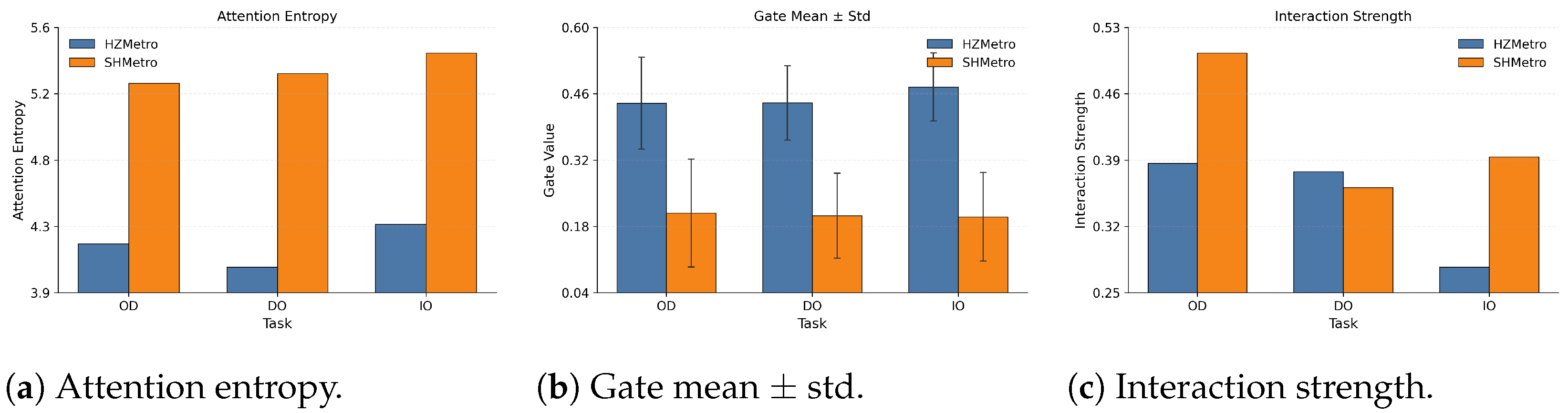
To better understand the behavior of CATI, we analyze the learned cross-task attention, gating, and interaction strength based on the trained model during inference. The corresponding statistics on HZMetro and SHMetro are shown in Figure 5.

5.5.1. Attention Behavior

Figure 5a presents the entropy of cross-task attention distributions. In both datasets, IO shows the highest entropy, indicating that it integrates information from a broader context than OD and DO. By contrast, OD and DO exhibit lower entropy values, reflecting more selective attention over informative source tasks. The relative ordering of OD and DO, however, is dataset-dependent: DO has the lowest entropy on HZMetro, while OD has the lowest entropy on SHMetro. This suggests that the concentration of cross-task interaction is not fixed, but adapts to the data characteristics of each metro system. Moreover, SHMetro consistently yields higher entropy than HZMetro across all tasks, indicating more distributed attention patterns under more heterogeneous flow conditions.

5.5.2. Gate Behavior

Figure 5b reports the mean and standard deviation of the learned gating values. On HZMetro, gate values remain moderate (≈0.44–0.48) with noticeable variability, reflecting the model’s ability to adaptively adjust the strength of cross-task signals. On SHMetro, the average gate values are lower (≈0.20–0.21), indicating a more conservative injection of auxiliary information, while the variance remains significant, suggesting that gating dynamically responds to different inputs. The variability of gating values shows task- and dataset-dependent patterns. On HZMetro, IO exhibits slightly higher variability compared to OD and DO, whereas on SHMetro, DO shows the largest variability among the three tasks. This indicates that the reliance on cross-task information is not fixed, but adapts to both task characteristics and dataset complexity.

5.5.3. Interaction Strength

Figure 5c quantifies the magnitude of injected cross-task information. OD consistently receives the strongest interaction signals across both datasets, indicating its central role in cross-task information aggregation. However, the relative ordering of DO and IO differs across datasets. On HZMetro, DO exhibits slightly stronger interaction than IO, whereas on SHMetro, IO surpasses DO. This suggests that the distribution of interaction strength is dataset-dependent and adapts to different flow characteristics. Overall, these results demonstrate that the model not only selects relevant information via attention but also modulates its contribution according to both task roles and dataset complexity, rather than applying a fixed interaction pattern.

5.5.4. Interpretability and Mobility Insights

Taken together, these observations reveal that CATI does not rely on uniform feature sharing across tasks. Instead, it performs selective interaction through attention mechanisms and regulates information integration via gating. Moreover, the model adapts its behavior to dataset characteristics. On SHMetro, attention distributions are generally more diffuse, and gating values are lower, indicating more cautious integration of cross-task information under heterogeneous conditions. In contrast, HZMetro exhibits more concentrated attention patterns, suggesting more focused information selection. At the same time, the distribution of interaction strength varies across tasks and datasets, reflecting task- and data-dependent prioritization of information flow. Overall, Figure 5 provides a form of structural and functional interpretability at the model level, showing that the performance gains of CATI stem from structured, adaptive, and data-dependent cross-task information propagation rather than simple feature fusion.

Beyond providing model-level interpretability, the observed interaction patterns reveal meaningful insights into real-world passenger flow dynamics. In particular, the attention distributions and interaction strengths learned by CATI reflect how different components of the metro system contribute to overall flow propagation. For example, the more concentrated attention patterns observed in HZMetro suggest that passenger movements are dominated by a limited number of major travel corridors, indicating a relatively centralized mobility structure. In contrast, the more diffuse attention distributions in SHMetro imply a more complex and distributed travel network, where passenger flows are spread across multiple alternative routes. This difference aligns with the distinct network scales and operational characteristics of the two metro systems. Furthermore, the variation in interaction strength across tasks indicates that the coupling between station-level flows (IO) and inter-station movements (OD/DO) is not uniform, but dynamically adjusted according to demand conditions. Stronger interactions correspond to periods of coordinated, system-wide travel demand (e.g., peak-hour commuting), while weaker interactions reflect more localized and less structured travel patterns during off-peak periods. These findings suggest that the proposed cross-task interaction mechanism does not merely improve predictive performance, but also captures interpretable mobility patterns that are consistent with real-world metro operations. This provides a potential pathway for bridging data-driven modeling and transportation system understanding.

6. Conclusions

In this work, we propose CATI, a cross-attention-based multi-task framework for metro passenger flow forecasting. The model captures task-specific spatiotemporal patterns and enables structured cross-task interaction, while gated residuals and pre-fusion design help control the flow of auxiliary information. Aggregation-consistency regularization further encourages coherence across tasks. Extensive experiments on HZMetro and SHMetro demonstrate that CATI consistently outperforms state-of-the-art baselines across multiple prediction horizons and tasks. Ablation studies show that cross-task interaction is the primary driver of performance gains, with gated residuals and pre-fusion improving stability, and consistency serving as an auxiliary structural constraint. Hyperparameter analysis confirms that the model is robust to reasonable variations in layer depth, encoding dimensions, and cross-attention capacity. Mechanism analysis provides interpretable insights, revealing that CATI achieves task-dependent selective attention, adaptive gating, and controlled interaction strength, adjusting to both task characteristics and dataset heterogeneity.

Despite these strengths, several limitations remain. First, CATI assumes a fixed set of tasks and may not generalize directly to scenarios with dynamically changing or newly added tasks. Second, the current cross-task interaction relies on pre-defined spatiotemporal embeddings, which may limit adaptation to highly heterogeneous or rapidly evolving urban systems. Third, while the gated residual and consistency mechanisms stabilize predictions, their hyperparameter tuning can be dataset-specific, potentially affecting deployment in new cities without additional validation. For future work, we plan to explore dynamic task adaptation to handle new or evolving tasks and to integrate adaptive spatiotemporal embeddings or graph structures learned from real-time data. Additionally, extending CATI to incorporate external factors, such as special events, weather, or transport disruptions, could further improve robustness and applicability in practical metro forecasting scenarios.

References

1. Shen, L.; Li, J.; Chen, Y.; Li, C.; Chen, X.; Lee, D.H. Short-Term Metro Origin–Destination Passenger Flow Prediction via Spatio-Temporal Dynamic Attentive Multi-Hypergraph Network. IEEE Trans. Intell. Transp. Syst. 2024, 25, 9945–9957. [Google Scholar] [CrossRef]
2. Hyun, J.; Joe, H.; Lee, C.; Kim, Y.R.; Lee, S. Optimizing Extended Metro Timetables During Year-End Events Using Graph Neural Networks: A Study on Passenger Flow Prediction and Timetable Optimization. IEEE Trans. Intell. Transp. Syst. 2025, 26, 15951–15961. [Google Scholar] [CrossRef]
3. Gao, C.; Liu, H.; Huang, J.; Wang, Z.; Li, X.; Li, X. Regularized Spatial–Temporal Graph Convolutional Networks for Metro Passenger Flow Prediction. IEEE Trans. Intell. Transp. Syst. 2024, 25, 11241–11255. [Google Scholar] [CrossRef]
4. Gao, Q.; Wang, Z.; Huang, L.; Trajcevski, G.; Liu, G.; Li, X. Responsive Dynamic Graph Disentanglement for Metro Flow Forecasting. Proc. Aaai Conf. Artif. Intell. 2025, 39, 11690–11698. [Google Scholar] [CrossRef]
5. Lv, S.; Wang, K.; Yang, H.; Wang, P. An Origin–Destination Passenger Flow Prediction System Based on Convolutional Neural Network and Passenger Source-Based Attention Mechanism. Expert Syst. Appl. 2024, 238, 121989. [Google Scholar] [CrossRef]
6. Liu, Y.; Chen, B.; Zheng, Y.; Cheng, L.; Li, G.; Lin, L. ODMixer: Fine-Grained Spatial-Temporal MLP for Metro Origin-Destination Prediction. IEEE Trans. Knowl. Data Eng. 2025, 37, 5508–5521. [Google Scholar] [CrossRef]
7. Liu, L.; Zhu, Y.; Li, G.; Wu, Z.; Bai, L.; Lin, L. Online Metro Origin–Destination Prediction via Heterogeneous Information Aggregation. IEEE Trans. Pattern Anal. Mach. Intell. 2023, 45, 3574–3589. [Google Scholar] [CrossRef] [PubMed]
8. Xu, Y.; Lyu, Y.; Xiong, G.; Wang, S.; Wu, W.; Cui, H.; Luo, J. Adaptive Feature Fusion Networks for Origin–Destination Passenger Flow Prediction in Metro Systems. IEEE Trans. Intell. Transp. Syst. 2023, 24, 5296–5312. [Google Scholar] [CrossRef]
9. Huang, H.; Mao, J.; Liu, R.; Lu, W.; Tang, T.; Liu, L. MTLMetro: A Deep Multi-Task Learning Model for Metro Passenger Demands Prediction. IEEE Trans. Intell. Transp. Syst. 2024, 25, 11805–11820. [Google Scholar] [CrossRef]
10. Li, P.; Wang, S.; Zhao, H.; Yu, J.; Hu, L.; Yin, H.; Liu, Z. IG-Net: An Interaction Graph Network Model for Metro Passenger Flow Forecasting. IEEE Trans. Intell. Transp. Syst. 2023, 24, 4147–4157. [Google Scholar] [CrossRef]
11. Liu, L.; Chen, J.; Wu, H.; Zhen, J.; Li, G.; Lin, L. Physical–Virtual Collaboration Modeling for Intra- and Inter-Station Metro Ridership Prediction. IEEE Trans. Intell. Transp. Syst. 2022, 23, 3377–3391. [Google Scholar] [CrossRef]
12. He, Y.; Li, L.; Zhu, X.; Tsui, K.L. Multi-Graph Convolutional–Recurrent Neural Network (MGC-RNN) for Short-Term Forecasting of Transit Passenger Flow. IEEE Trans. Intell. Transp. Syst. 2022, 23, 18155–18174. [Google Scholar] [CrossRef]
13. Zhao, Y.; Lin, Y.; Zhang, Y.; Wen, H.; Liu, Y.; Wu, H.; Wu, Z.; Zhang, S.; Wan, H. Traffic Inflow and Outflow Forecasting by Modeling Intra- and Inter-Relationship Between Flows. IEEE Trans. Intell. Transp. Syst. 2022, 23, 20202–20216. [Google Scholar] [CrossRef]
14. Xie, P.; Ma, M.; Li, T.; Ji, S.; Du, S.; Yu, Z.; Zhang, J. Spatio-Temporal Dynamic Graph Relation Learning for Urban Metro Flow Prediction. IEEE Trans. Knowl. Data Eng. 2023, 35, 9973–9984. [Google Scholar] [CrossRef]
15. Ma, M.; Hu, J.; Jensen, C.S.; Teng, F.; Han, P.; Xu, Z.; Li, T. Learning Time-Aware Graph Structures for Spatially Correlated Time Series Forecasting. In Proceedings of the 2024 IEEE 40th International Conference on Data Engineering (ICDE), Utrecht, The Netherlands, 13–16 May 2024; pp. 4435–4448. [Google Scholar] [CrossRef]
16. Liu, W.; Li, H.; Zhang, H.; Xue, J.; Sun, S. Dynamic Spatio-Temporal Graph Fusion Network Modeling for Urban Metro Ridership Prediction. Inf. Fusion 2025, 117, 102845. [Google Scholar] [CrossRef]
17. Ye, X.; Fang, S.; Sun, F.; Zhang, C.; Xiang, S. Meta Graph Transformer: A Novel Framework for Spatial–Temporal Traffic Prediction. Neurocomputing 2022, 491, 544–563. [Google Scholar] [CrossRef]
18. Zhang, J.; Mao, S.; Zhang, S.; Yin, J.; Yang, L.; Gao, Z. EF-former for short-term passenger flow prediction during large-scale events in urban rail transit systems. Inf. Fusion 2025, 117, 102916. [Google Scholar] [CrossRef]
19. Wu, J.; He, D.; Jin, Z.; Li, X.; Li, Q.; Xiang, W. Learning spatial–temporal pairwise and high-order relationships for short-term passenger flow prediction in urban rail transit. Expert Syst. Appl. 2024, 245, 123091. [Google Scholar] [CrossRef]
20. Li, H.; Fu, W.; Zhang, H.; Liu, W.; Sun, S.; Zhang, T. Spatio–temporal graph hierarchical learning framework for metro passenger flow prediction across stations and lines. Knowl.-Based Syst. 2025, 311, 113132. [Google Scholar] [CrossRef]
21. Dong, H.; Ding, F.; Tan, H.; Wu, Y.; Ran, B. Rail Transit OD-Matrix Completion via Manifold Regularised Tensor Factorisation. IET Intell. Transp. Syst. 2021, 15, 1304–1317. [Google Scholar] [CrossRef]
22. Jiang, W.; Ma, Z.; Koutsopoulos, H.N. Deep learning for short-term origin–destination passenger flow prediction under partial observability in urban railway systems. Neural Comput. Appl. 2022, 34, 4813–4830. [Google Scholar] [CrossRef]
23. Huang, J.; Huang, B.; Yu, W.; Xiao, J.; Xie, R.; Ruan, K. ODformer: Spatial–Temporal Transformers for Long Sequence Origin–Destination Matrix Forecasting Against Cross Application Scenario. Expert Syst. Appl. 2023, 226, 119835. [Google Scholar] [CrossRef]
24. Zhang, Y.; Sun, K.; Wen, D.; Chen, D.; Lv, H.; Zhang, Q. Deep Learning for Metro Short-Term Origin-Destination Passenger Flow Forecasting Considering Section Capacity Utilization Ratio. IEEE Trans. Intell. Transp. Syst. 2023, 24, 7943–7960. [Google Scholar] [CrossRef]
25. Vaswani, A.; Shazeer, N.; Parmar, N.; Uszkoreit, J.; Jones, L.; Gomez, A.N.; Kaiser, Ł.; Polosukhin, I. Attention is All you Need. In Advances in Neural Information Processing Systems; Curran Associates, Inc.: Red Hook, NY, USA, 2017; Volume 30, pp. 6000–6010. [Google Scholar]
26. Li, Y.; Yu, R.; Shahabi, C.; Liu, Y. Diffusion Convolutional Recurrent Neural Network: Data-Driven Traffic Forecasting. In Proceedings of the 6th International Conference on Learning Representations, ICLR 2018, Vancouver, BC, Canada, 30 April–3 May 2018. [Google Scholar]
27. Wu, Z.; Pan, S.; Long, G.; Jiang, J.; Zhang, C. Graph WaveNet for Deep Spatial-Temporal Graph Modeling. In Proceedings of the Twenty-Eighth International Joint Conference on Artificial Intelligence, IJCAI 2019, Macao, China, 10–16 August 2019; pp. 1907–1913. [Google Scholar] [CrossRef]
28. Shang, C.; Chen, J.; Bi, J. Discrete Graph Structure Learning for Forecasting Multiple Time Series. In Proceedings of the 9th International Conference on Learning Representations, ICLR 2021, Virtual Event, 3–7 May 2021. [Google Scholar]
29. Zhou, H.; Zhang, S.; Peng, J.; Zhang, S.; Li, J.; Xiong, H.; Zhang, W. Informer: Beyond Efficient Transformer for Long Sequence Time-Series Forecasting. Proc. Aaai Conf. Artif. Intell. 2021, 35, 11106–11115. [Google Scholar] [CrossRef]
30. Liu, H.; Dong, Z.; Jiang, R.; Deng, J.; Deng, J.; Chen, Q.; Song, X. Spatio-Temporal Adaptive Embedding Makes Vanilla Transformer SOTA for Traffic Forecasting. In Proceedings of the 32nd ACM International Conference on Information and Knowledge Management (CIKM ’23), Birmingham, UK, 21–25 October 2023; pp. 4123–4129. [Google Scholar] [CrossRef]
Figure 1. The CATI framework. Arrows indicate flow direction.
Symmetry 18 00809 g001
Figure 2. Task-specific encoding with OD completion and cross-task interaction module. Arrows indicate flow direction; arrow colors distinguish different streams.
Symmetry 18 00809 g002
Figure 3. Task-specific encoding and cross-task interaction module. Arrows indicate flow direction; arrow colors distinguish different streams.
Symmetry 18 00809 g003
Figure 4. Cross-Attention and Gated Residual Fusion (CAGRF) module.
Symmetry 18 00809 g004
Figure 5. Cross-dataset comparison of key mechanism statistics in CATI. (a) Attention entropy across tasks, where lower entropy indicates more concentrated cross-task selection. (b) Gate mean with standard deviation, showing adaptive modulation of injected information. (c) Interaction strength across tasks, measuring the magnitude of cross-task signals injected into task representations. Results are reported on HZMetro and SHMetro using the trained model during inference.
Symmetry 18 00809 g005