Effective Potentials for de Sitter and Anti-de Sitter Quantum Fields

Abstract

We derive a systematic treatment of one-loop effective potentials for interacting scalar fields in curved spacetimes, providing a general formula valid in arbitrary geometries and explicit results for de Sitter and anti-de Sitter backgrounds. We then compute the effective potential for a scalar $O\left(N\right)$ theory on a de Sitter space in any integer dimension. In $d=3$ and dimensional regularization, we extend the calculation up to two-loops and compute the $\beta$-function and the anomalous mass dimension. They coincide exactly with flat-space results, despite dramatic curvature modifications to physical masses/couplings. The flat limit $R\to \infty$ recovers Coleman–Weinberg, confirming consistency. Working in $d=3$ dimension, we repeat the calculation for $Ad{S}_3$ by using point-splitting regularization, obtaining analogue results for the $\beta$-function and anomalous mass dimension (Dedicated to Jean Pierre Gazeau on his 80th Birthday).

1. Introduction

Effective potentials in quantum field theory (QFT) are a central tool to incorporate quantum corrections into classical potentials, allowing precise analyses of vacuum stability [1,2], radiative symmetry breaking (as in the Coleman–Weinberg mechanism [3]), phase transitions and critical phenomena [4,5,6], as well as applications such as electroweak metastability [7] or Higgs-driven inflation [8]. In this framework, quantum loop effects are encoded in a field-dependent potential whose minima identify the true quantum vacua, and which provides a compact way of organizing radiative corrections in situations where constant or slowly varying background fields play a distinguished role.

In flat Minkowski space, the diagrammatic structure and renormalization of the effective potential are by now standard material, and efficient techniques exist to compute it to high loop order and to resum large logarithms in a controlled way. But realistic phenomena typically unfold in gravitational backgrounds and therefore it is desirable to generalize effective potentials from flat Minkowski space to curved spacetimes [9,10,11]. Situations of interest include inflationary dynamics in de Sitter (dS) space, quantum fields around black holes, and physics near cosmological horizons, where curvature effects qualitatively modify quantum fluctuations and can render flat-space approximations unreliable.

De Sitter space in particular plays a distinguished role both as an approximate description of the inflationary epoch [12] and as a model of the present accelerated universe, while anti-de Sitter (AdS) space is central to holographic dualities and strongly coupled systems [13]. In all these contexts, a consistent treatment of the effective potential in the presence of curvature is needed to address questions of vacuum structure, symmetry-breaking patterns, and phase transitions in a genuinely gravitational setting, and to assess, for instance, the stability of metastable vacua in the early universe or in curved backgrounds relevant for high-energy physics.

Extending the effective potential to curved backgrounds entails both technical and conceptual difficulties. In curved spacetime, the notions of vacuum and particle states become considerably more subtle, particularly in the absence of a global timelike Killing vector, as in the de Sitter case, and even more so when the manifold fails to be globally hyperbolic, as occurs for AdS. Fortunately, in both de Sitter and anti-de Sitter spacetimes, one can adopt a formulation based on maximally analytic two-point functions defined on their complexified manifolds. This framework effectively replaces the usual spectral condition—which cannot be consistently implemented in de Sitter quantum field theory—as well as the standard boundary conditions imposed on modes in the anti-de Sitter setting [14,15,16,17]. Our analysis will rely heavily on this approach.

In curved spacetime, loop integrals involve Feynman or Schwinger functions defined on non-trivial manifolds and must be regularized and renormalized in a manner consistent with the underlying geometry and its symmetries. The presence of curvature introduces additional couplings, such as the non-minimal interaction term $\xi R{\phi }^2$, and leads to a non-trivial interplay between mass parameters, curvature couplings, and the cosmological constant.

In many practical applications, one relies on ad hoc extensions of flat-space expressions. However, a systematic derivation valid for general curved backgrounds is less commonly developed. It is therefore desirable to construct a formulation of the effective potential that remains as close as possible to standard flat-space diagrammatic techniques, while being consistently adapted to curved manifolds such as spherical and hyperbolic spaces.

The purpose of this work is twofold. First, we derive a general expression for the one-loop effective potential valid in arbitrary Euclidean curved spacetimes, under a mild condition on the Laplacian acting on two-edge-connected diagrams. Starting from the Coleman–Weinberg observation that the effective potential admits a diagrammatic expansion as the sum of all one-particle-irreducible (1PI) graphs with vanishing external momenta [3], we show that polygon vacuum diagrams constructed from Schwinger propagators can be systematically reduced to derivatives of the tadpole diagram with respect to the bare mass squared. This procedure leads to curved-space analogues of relations previously identified in flat space by Lee and Sciaccaluga [18], and culminates in a compact equation expressing the derivative of the effective potential with respect to the field-dependent mass in terms of the coincident propagator. We prove that this relation holds on any Euclidean background for which a simple Laplacian identity for two-edge-connected diagrams is satisfied. Our primary examples include the Euclidean de Sitter sphere $S_d$, the Lobachevsky (Euclidean AdS) manifold $H_d$, and their common flat limit, Euclidean space $E_d$.

Second, we apply this general framework to a concrete and physically rich class of models: real scalar fields with quartic self-interaction on de Sitter and anti-de Sitter backgrounds, with particular emphasis on three dimensions. For the $O\left(N\right)$ model on the Euclidean de Sitter sphere $S_d$, we employ the maximally analytic two-point function [14,15] and its restriction to the sphere to compute the dimensionally regularized tadpole and, via our general formula, the one-loop effective potential in arbitrary spacetime dimension. Interestingly enough, our formula for the one-loop effective potential can be applied to more general contexts where the Schwinger function can be determined exactly or perturbatively. For example, for Schwarzschild–de Sitter black holes modeling primordial black holes in applications to cosmology, see, e.g., [19], or to study the thermodynamic aspects at the near horizon of black holes or black branes [20].

We then focus on $d=3$, where the model is super-renormalizable and directly relevant to statistical and condensed-matter physics, since lower-dimensional quantum field theories often provide effective descriptions of critical phenomena and universality classes [4,5,6]. In this three-dimensional de Sitter background, we go beyond one-loop and compute the effective potential at two-loops, combining our tadpole-based method with the explicit expressions for banana integrals recently obtained in de Sitter space [21].

This procedure yields a fully renormalized two-loop effective potential in ${dS}_3$ and allows us to clarify in detail how mass and cosmological-constant renormalization operates in this geometry. In particular, we show that the soft divergences characteristic of super-renormalizable theories are absorbed entirely by mass renormalization, while finite curvature-dependent contributions modify the effective cosmological constant and may be interpreted as radiative shifts in the gravitational sector.

In this case, we worked with the dimensional regularization scheme, where, in $d=3$, only logarithmic divergences appear, from which the renormalization flux and the anomalous mass dimension can be directly read. However, it is remarkable to notice that if one works at $d=3$ with a cut-off regularization, then the direct calculation of the effective potential up to two-loops becomes almost elementary, with the small price of introducing non-logarithmic divergences already at one-loop level. In order to illustrate this fact, we turn to the analogous $O\left(N\right)$ model on ${AdS}_3$, where we compute the effective potential up to two-loops using point-splitting regularization rather than dimensional regularization. In this setting the Euclidean propagator admits a particularly simple representation, which enables an explicit evaluation of the two-loop “watermelon” diagrams in terms of elementary functions and hypergeometric integrals. The computation exploits a Källén–Lehmann-type spectral decomposition on the Lobachevsky manifold [16,22,23], rendering the relevant convolution integrals tractable.

While the renormalization scheme and intermediate expressions differ substantially from the de Sitter case, the final renormalization-group data are remarkably robust. In particular, the anomalous mass dimension and the beta function for a suitably defined dimensionless coupling coincide with their flat-space counterparts, in agreement with general expectations for super-renormalizable theories in three dimensions [24].

By contrast, the relation between renormalized parameters $(m,c)$ and physical quantities, such as the pole mass and physical coupling $(m_{\mathrm{phys}},c_{\mathrm{phys}})$, as well as the cosmological constant, is nontrivially affected by curvature in both dS and AdS. In the weak-curvature limit we explicitly recover the known flat-space two-loop effective potential in $d=3$ [24]. Furthermore, our analysis cleanly disentangles the purely kinematical mass renormalization from genuine curvature-induced contributions, which effectively generate a non-minimal coupling to the background geometry.

From a conceptual standpoint, our analysis highlights how curvature enters the effective potential in multiple ways. In de Sitter space, the same quantum fluctuations that renormalize the mass and quartic coupling also induce finite corrections to the cosmological constant, which can be interpreted as radiative shifts to Newton’s constant when the de Sitter radius is treated as a renormalized parameter. In three dimensions, where logarithmic divergences are absent at one-loop but appear at two-loops, these corrections translate into a curvature-dependent separation between the “kinematical” mass and the effective nonminimal $\xi R{\varphi }^2$ coupling; in the weak-gravity regime this separation can be made explicit, and one can track how the physical mass receives both flat-space and curvature-induced contributions. In ${AdS}_3$, similar considerations apply, although the ultraviolet structure is organized in terms of the point-splitting scale rather than the dimensional regulator, and the spectrum of fluctuations reflects the different global geometry and boundary conditions.

Finally, our results fit naturally into the broader program of using lower-dimensional QFTs as laboratories for critical phenomena and for quantum fields in curved space. Three-dimensional scalar theories with $O\left(N\right)$ symmetry provide prototypical examples for universality classes relevant to statistical systems near criticality [4,5,6], and the inclusion of de Sitter or anti-de Sitter curvature opens the way to controlled studies of how gravitational backgrounds distort or shift phase structure and critical behaviour. The explicit two-loop effective potentials we obtain in ${\mathrm{dS}}_3$ and ${\mathrm{AdS}}_3$ offer a concrete starting point for such investigations, including radiative symmetry breaking, metastability, and curvature-induced transitions. They may also be useful in future work on holographic interpretations of scalar effective actions in AdS and on stochastic or infrared approaches to scalar fields in de Sitter space.

The paper is organized as follows. In Section 2, we revisit the diagrammatic expansion of the effective potential and derive a general formula relating polygon vacuum diagrams to derivatives of the tadpole on curved Euclidean backgrounds satisfying a simple Laplacian identity. This leads to a compact expression for the one-loop effective potential in terms of the coincident Schwinger function and generalizes the Lee–Sciaccaluga equation to curved space. In Section 3, we apply this framework to the $O\left(N\right)$ model on the Euclidean de Sitter sphere, compute the one-loop effective potential in arbitrary dimension, and carry out a full two-loop calculation in three dimensions, including a detailed discussion of renormalization, physical parameters, and the flat limit. In Section 4, we perform the analogous analysis for $Ad{S}_3$, using point-splitting regularization to evaluate the relevant loop integrals and to obtain the two-loop effective potential and renormalization conditions.

2. The 1-Loop Effective Potential in Curved Spacetime: A General Formula

In 1973 Coleman and Weinberg [3] pointed out that there exists a diagrammatic expansion for the effective potential: it is the sum of all 1PI graphs with vanishing external momenta. At one-loop, for a scalar field with quartic self-interaction, this amounts to the sum of all polygonal diagrams built with the free Feynman propagator:

$$\begin{array}{c}\hfill V\left(\phi \right)={\displaystyle \frac{1}{2}}{m}^2{\phi }^2+{\displaystyle \frac{c}{4}}{\phi }^4+V_0\left(\phi \right)={\displaystyle \frac{1}{2}}{m}^2{\phi }^2+{\displaystyle \frac{c}{4}}{\phi }^4+i{\displaystyle \sum _{n=1}^{\infty }}{\displaystyle \frac{{\left(3c{\phi }^2\right)}^n}{2n}}\int {\displaystyle \frac{d^{4}k}{{\left(2\pi \right)}^4}}{\displaystyle \frac{1}{{(k^2-m^2+iϵ)}^n}};\end{array}$$

(1)

here we leave all counterterms aside.

In their seminal paper Coleman and Weinberg discussed the case where the bare mass m is zero, but the presence of a non-zero mass m, as in the above formula, is helpful. Let us consider indeed the tadpole diagram, which formally amounts to the value at coinciding points of the propagator:

$$\begin{array}{c}\hfill G\left(0\right)=\int {\displaystyle \frac{d^{4}k}{{\left(2\pi \right)}^4}}{\displaystyle \frac{1}{(k^2-m^2+iϵ)}};\end{array}$$

(2)

by using the elementary formal identity

$$\begin{array}{c}\hfill \int {\displaystyle \frac{d^{4}k}{{\left(2\pi \right)}^4}}{\displaystyle \frac{1}{{(k^2-m^2+iϵ)}^{n+1}}}={\displaystyle \frac{1}{n!}}{\left({\displaystyle \frac{\partial }{\partial m^2}}\right)}^{n}G\left(0\right)\end{array}$$

(3)

it is possible to reshape Equation (1) as follows:

$$\begin{array}{c}\hfill V\left(\phi \right)={\displaystyle \frac{1}{2}}{m}^2{\phi }^2+{\displaystyle \frac{c}{4}}{\phi }^4+i{\displaystyle \sum _{n=1}^{\infty }}{\displaystyle \frac{{\left(3c{\phi }^2\right)}^n}{2n}}{\displaystyle \frac{1}{(n-1)!}}{\displaystyle \frac{{\partial }^{n-1}}{{(\partial m^2)}^{n-1}}}G\left(0\right).\end{array}$$

(4)

We aim to demonstrate that Equation (4) enjoys significantly broader applicability beyond flat spacetime. Our primary examples comprise the de Sitter sphere $S_d$, the Lobachevsky (Euclidean AdS) manifold $H_d$, and their shared flat limit, the Euclidean space $E_d$; the framework, however, remains more general.

Consider a two-edge connected diagram featuring two distinct external vertices in a d-dimensional Euclidean curved manifold ${\mathcal{E}}_d$:

$$\begin{array}{c}\hfill F_{m_1{m}_2}(x,y)={\int }_{{\mathcal{E}}_d}{S}_{m_1}(x,z)S_{m_2}(y,z)\sqrt{g\left(z\right)}dz,\end{array}$$

(5)

where $S_{m_i}(x,y)$ denote the corresponding Schwinger propagators, with distinct masses $m_1\ne m_2$. The distribution $F_{m_1{m}_2}(x,y)$ is a joint solution of the following equations:

$$\begin{array}{ccc}& & (-{\nabla }_x^2+m_1^2)F_{m_1{m}_2}(x,y)=\int \delta (z,x)S_{m_2}(z,y)\sqrt{g\left(z\right)}dz=S_{m_2}(x,y),\hfill \end{array}$$

(6)

$$\begin{array}{ccc}& & (-{\nabla }_y^2+m_2^2)F_{m_1{m}_2}(x,y)=\int S_{m_1}(x·z)\delta (y,z)\sqrt{g\left(z\right)}dz=S_{m_1}(x·y).\hfill \end{array}$$

(7)

Suppose that

$$\begin{array}{c}\hfill {\nabla }_x^2{F}_{m_1{m}_2}(x,y)={\nabla }_y^2{F}_{m_1{m}_2}(x,y).\end{array}$$

(8)

This condition holds in particular in de Sitter, anti-de Sitter, and flat spacetimes.

Subtracting Equation (7) from Equation (6) shows that the above two-edge diagram reduces to a linear combination of free propagators:

$$\begin{array}{c}\hfill F_{m_1{m}_2}(x,y)=-{\displaystyle \frac{S_{m_1}(x,y)}{m_1^2-m_2^2}}-{\displaystyle \frac{S_{m_2}(x,y)}{m_2^2-m_1^2}}.\end{array}$$

(9)

In the limit $m_1\to m_2$, this expression becomes the derivative of the propagator with respect to $m^2$:

$$\begin{array}{ccc}& & F_{m\left(2\right)}(x,y)=-{\displaystyle \frac{\partial }{\partial m^2}}{S}_m(x,y).\hfill \end{array}$$

(10)

By taking the limit $y\to x$ in Equation (9), we deduce a general formula for the bubble vacuum diagram:

$$\begin{array}{c}\hfill bubble(m_1,m_2)={\int }_{{\mathcal{E}}_d}{S}_{m_1}(x,z)S_{m_2}(z,x)\sqrt{g\left(z\right)}dz=-{\displaystyle \frac{S_{m_1}(x,x)-S_{m_2}(x,x)}{m_1^2-m_2^2}}.\end{array}$$

(11)

In particular, for equal masses

$$\begin{array}{c}\hfill bubble\left(m\right)=-{\displaystyle \frac{\partial }{\partial m^2}}{S}_m(x,x)=-{\displaystyle \frac{\partial }{\partial m^2}}tadpole\left(m\right).\end{array}$$

(12)

Iterating the above construction, always supposing the validity of Equation (8), we compute the 3-edge diagram with two internal vertices as follows:

$$\begin{array}{cc}{F}_{m_1{m}_2{m}_3}(x,y)& ={\int }_{{\mathcal{E}}_d\times {\mathcal{E}}_d}{S}_{m_1}(x,x_1)S_{m_2}(x_1,x_2)S_{m_3}(x_2,y)\sqrt{g\left(x_1\right)}d{x}_1\sqrt{g\left(x_2\right)}d{x}_2\hfill \\ & ={\displaystyle \frac{S_{m_1}(x,y)}{(m_1^2-m_2^2)(m_1^2-m_3^2)}}+{\displaystyle \frac{S_{m_2}(x,y)}{(m_2^2-m_3^2)(m_2^2-m_1^2)}}+{\displaystyle \frac{S_{m_3}(x,y)}{(m_3^2-m_1^2)(m_3^2-m_2^2)}};\hfill \end{array}$$

(13)

for equal masses this reduces to

$$\begin{array}{c}\hfill F_{m\left(3\right)}(x,y)={\displaystyle \frac{1}{2}}{\left({\displaystyle \frac{\partial }{\partial m^2}}\right)}^2{S}_m(x,y).\end{array}$$

(14)

The limit $y\to x$ gives the triangle diagrams with vanishing external momenta. In particular when the three masses are equal

$$\begin{array}{c}\hfill triangle\left(m\right)={\displaystyle \frac{1}{2}}{\left({\displaystyle \frac{\partial }{\partial m^2}}\right)}^{2}tadpole\left(m\right).\end{array}$$

(15)

In general, we may compute the $(n+1)$-edge diagram with n-internal vertices and get the following linear combination of propagators:

$$\begin{array}{cc}\hfill F_{m_1{m}_2,\dots ,m_n}(x,y)& ={\int }_{{\mathcal{E}}_d}{S}_{m_1}(x,x_1)\dots S_{m_j}(x_n,y)\sqrt{g\left(x_1\right)}d{x}_1\dots \sqrt{g\left(x_n\right)}d{x}_n\hfill \\ & ={(-1)}^n{\displaystyle \sum _{j=1}^n}{\displaystyle \frac{S_{m_j}(x,y)}{{\prod }_{i\ne j}(m_j^2-m_i^2)}}.\hfill \end{array}$$

(16)

If the masses circulating in the diagram are all equal, this formula reduces to

$$\begin{array}{c}\hfill F_{m\left(n\right)}(x,y)={\displaystyle \frac{{(-1)}^n}{n!}}{\left({\displaystyle \frac{\partial }{\partial m^2}}\right)}^n{S}_m(x,y).\end{array}$$

(17)

The polygon vacuum diagram with $(n+1)$ propagators is obtained by taking the limit $y\to x$ and is proportional to the n-th derivative of the tadpole w.r.t. the bare mass squared:

$$\begin{array}{c}\hfill polygo{n}_{n+1}\left(m\right)={\displaystyle \frac{{(-1)}^n}{n!}}{\left({\displaystyle \frac{\partial }{\partial m^2}}\right)}^{n}tadpole\left(m\right).\end{array}$$

(18)

This formula provides a generalization of Equation (3) and is a consequence of the more general Equation (16). Equations (16) and (18) are true on any curved background with Euclidean signature (similar formulae exists also for the chronological propagator in Lorentzian signature) provided the identity (8) holds; in particular they hold for the flat, spherical, and hyperbolic Euclidean geometries. The coincident-vertex limit is typically divergent, requiring regularization and renormalization; in the following we will explore both the dimensional and the UV cutoff regularizations.

Let us now consider the 1-loop correction in Equation (4)

$$\begin{array}{c}\hfill V_0\left(\phi \right)={\displaystyle \sum _{n=1}^{\infty }}{\displaystyle \frac{1}{2n(n-1)!}}{\left(3c{\phi }^2\right)}^n{\left({\displaystyle \frac{\partial }{\partial m^2}}\right)}^{n-1}{S}_m(x,x)\end{array}$$

(19)

and take the derivative of both sides with respect to $\phi$:

$$\begin{array}{c}\hfill {\partial }_{\phi }{V}_0\left(\phi \right)=3c\phi {\displaystyle \sum _{n=1}^{\infty }}{\displaystyle \frac{1}{(n-1)!}}{\left(3c{\phi }^2\right)}^{n-1}{\left({\displaystyle \frac{\partial }{\partial m^2}}\right)}^{n-1}{S}_m(x,x)=3c\phi S_{M\left(\phi \right)}(x,x),\end{array}$$

(20)

where we have defined

$$M^2\left(\phi \right)=m^2+3c{\phi }^2.$$

(21)

It is useful to rewrite Equation (20) as follows:

$$\begin{array}{c}\hfill {\displaystyle \frac{\partial V_0\left(\phi \right)}{\partial M^2\left(\phi \right)}}={\displaystyle \frac{1}{2}}{S}_{M\left(\phi \right)}(x,x).\end{array}$$

(22)

In flat space, this is nothing but the Lee–Sciaccaluga equation for the effective potential [18]. Here, its validity has been established on an arbitrary curved background, provided that condition (8) is satisfied, and widely generalizes the results in [25], valid in homogeeous and globally static spacetimes. Moreover, the equation continues to hold to all orders in the loop expansion.

Let us show for instance how to recover the standard result of Coleman and Weinberg at 1-loop with the above formulae. The Schwinger propagator in flat space behaves at short distances as follows:

$$\begin{array}{c}\hfill S_m(x,y)={\displaystyle \frac{1}{{\left(2\pi \right)}^{\frac{d}{2}}}}{\left({\displaystyle \frac{r}{m}}\right)}^{1-{\displaystyle \frac{d}{2}}}{K}_{{\displaystyle \frac{d}{2}}-1}\left(mr\right)\simeq {\displaystyle \frac{r^{2-d}}{4{\pi }^{\frac{d}{2}}}}\mathrm{\Gamma }\left({\displaystyle \frac{d}{2}}-1\right)+{\displaystyle \frac{m^{d-2}}{{\left(4\pi \right)}^{\frac{d}{2}}}}\mathrm{\Gamma }\left(1-{\displaystyle \frac{d}{2}}\right)\end{array}$$

(23)

where $r=|x-y|$. For $d<2$, only the second term survives at $r=0$, yielding

$$\begin{array}{c}\hfill {\left({\displaystyle \frac{\partial }{\partial m^2}}\right)}^{n-1}{S}_m\left(0\right)={(-1)}^{n-1}{\displaystyle \frac{{\left(m^2\right)}^{\frac{d}{2}-n}}{{\left(4\pi \right)}^{\frac{d}{2}}}}\mathrm{\Gamma }\left(n-{\displaystyle \frac{d}{2}}\right).\end{array}$$

(24)

Inserting this expression into Equation (19) and carrying out the summation, we obtain—after analytic continuation—the one-loop contribution to the effective potential in closed form. The resulting expression is a simple meromorphic function of the spacetime dimension d:

$$\begin{array}{c}\hfill V_0\left(\phi \right)={\displaystyle \frac{1}{2^{1+d}{\pi }^{\frac{d}{2}}}}\mathrm{\Gamma }\left(-{\displaystyle \frac{d}{2}}\right)\left(m^d-{\left(m^2+3c{\phi }^2\right)}^{{\displaystyle \frac{d}{2}}}\right).\end{array}$$

(25)

Integrating Equation (22) obviously gives the same result provided the arbitrary constant term is fixed by requiring $V_0\left(0\right)=0$.

In odd dimensions, Equation (25) is already regular; in particular, in $d=1$ and $d=3$ we get

$$\begin{array}{ccc}& d=1:& V_0^{\left(1\right)}\left(\phi \right)={\displaystyle \frac{1}{2}}\left(\sqrt{m^2+3c{\phi }^2}-m\right),\hfill \end{array}$$

(26)

$$\begin{array}{ccc}& d=3:& V_0^{\left(3\right)}\left(\phi \right)={\displaystyle \frac{m^3-{\left(m^2+3c{\phi }^2\right)}^{3/2}}{12\pi }}.\hfill \end{array}$$

(27)

In even dimensions, Equation (25) is divergent and needs to be regularized and normalized to get the finite result. Let us extract formulae in $d=2-2ϵ$ and $d=4-2ϵ$. We may drop the constant term and get

$$\begin{array}{ccc}& d=2-2ϵ:& V_0^{\left(2\right)}\left(\phi \right)=\left({\displaystyle \frac{3(1-\gamma )+\log \left(64{\pi }^3\right)}{8\pi }}+{\displaystyle \frac{3}{2\pi ϵ}}\right){\phi }^2-{\displaystyle \frac{\left(m^2+3c{\phi }^2\right)\log \left(m^2+3c{\phi }^2\right)}{8\pi }}\hfill \\ & & +O\left(ϵ\right)\hfill \end{array}$$

(28)

$$\begin{array}{ccc}& d=4-2ϵ:& V_0^{\left(4\right)}\left(\phi \right)=-{\displaystyle \frac{1}{64{\pi }^2}}{\left(m^2+3c{\phi }^2\right)}^2\left({\displaystyle \frac{1}{ϵ}}+\log \left(4\pi \right)-\gamma \right)+\hfill \\ & & +{\displaystyle \frac{1}{64{\pi }^2}}{\left(m^2+3c{\phi }^2\right)}^2\left(\log \left(m^2+3c{\phi }^2\right)-{\displaystyle \frac{3}{2}}\right)+O\left(ϵ\right).\hfill \end{array}$$

(29)

In both cases the first term contributes to the renormalization of the bare tree-level constants. The remaining term reproduces the one-loop effective potential in $d=2,4$ for a real scalar field with quartic self-interaction [3,18].

3. The O(N) Model on the Euclidean de Sitter Sphere

Let us start by briefly recalling some facts about de Sitter (scalar) quantum fields. Let $M_{d+1}$ be the real $(d+1)$-dimensional Minkowski spacetime and $M_{d+1}^{\left(c\right)}$ be its complexification. In a chosen Lorentz frame the scalar product of two (complex) events is

$$z_1·z_2=z_1^0{z}_2^0-z_1^1{z}_2^1-\dots -z_1^d{z}_2^d.$$

(30)

The (complex) de Sitter universe may be represented as the one-sheeted hyperboloid immersed in the (complex) Minkowski space $M_{d+1}^{\left(c\right)}$:

$$d{S}_d^{\left(c\right)}=\{z\in M_{d+1}^{\left(c\right)}:z·z=-R^2\}.$$

(31)

The de Sitter invariant complex variable $\zeta$ is the scalar product in the ambient spacetime of two complex events $z_1,z_2\in d{S}_d^{\left(c\right)}$:

$$\zeta ={\displaystyle \frac{z_1·z_2}{R^2}}.$$

(32)

The future and past tuboids ${\mathcal{T}}_{\pm }$, which encode the spectral condition for quantum field theory on de Sitter space, are defined as the intersections of the ambient forward and backward tubes $T_{\pm }$ with the complexified de Sitter manifold:

$${\mathcal{T}}_{\pm }=\{x+iy\in d{S}_d^{\left(c\right)}:y\in \pm V_{+}\}.$$

(33)

Because de Sitter spacetime does not admit a global timelike Killing vector, a standard spectral condition cannot be formulated. Instead, one imposes the requirement of normal analyticity [14,15]: the two-point distributions must arise as boundary values of functions holomorphic in the domain ${\mathcal{T}}_{-}\times {\mathcal{T}}_{+}$. Combined with de Sitter invariance and the canonical commutation relations, this condition uniquely fixes the two-point function of any de Sitter massive Klein–Gordon field [14,15,21]:

$$\begin{array}{cc}\hfill W_{\nu }^d(z_1,z_2)& ={\displaystyle \frac{\mathrm{\Gamma }\left(\frac{d-1}{2}+i\nu \right)\mathrm{\Gamma }\left(\frac{d-1}{2}-i\nu \right)}{2{\left(2\pi \right)}^{d/2}}}{({\zeta }^2-1)}^{-{\displaystyle \frac{d-2}{4}}}{P}_{-{\displaystyle \frac{1}{2}}+i\nu }^{-{\displaystyle \frac{d-2}{2}}}\left(\zeta \right)\hfill \end{array}$$

(34)

$$\begin{array}{cc}\hfill & ={\displaystyle \frac{\mathrm{\Gamma }\left(\frac{d-1}{2}+i\nu \right)\mathrm{\Gamma }\left(\frac{d-1}{2}-i\nu \right)}{{\left(4\pi \right)}^{d/2}\mathrm{\Gamma }\left(\frac{d}{2}\right)}}{}_{2}F_1\left({\displaystyle \frac{d-1}{2}}+i\nu ,{\displaystyle \frac{d-1}{2}}-i\nu ;{\displaystyle \frac{d}{2}};{\displaystyle \frac{1-\zeta }{2}}\right).\hfill \end{array}$$

(35)

The complex parameter $\nu$ is related to the complex mass squared as follows:

$$m^2={\displaystyle \frac{{(d-1)}^2}{4}}+{\nu }^2.$$

(36)

The squared mass is real and positive only when:

• $\nu$ is real; this correspond in a group-theoretical language to the principal series of unitary representations of the Lorentz group;
• $\nu$ is purely imaginary such that $\left|\nu \right|<{\displaystyle \frac{d-1}{2}}$; this corresponds to the complementary series of unitary representations of the Lorentz group.

There is also a discrete series of acceptable QFTs with negative squared mass [26,27]. Finally, the Schwinger function (in short: the propagator) is the restriction of the maximally analytic two-point function to the Euclidean sphere

$$S_d=\{z_E\in d{S}_d^{\left(c\right)},z_E^0=i{x}^0,z_E^i=x^i,x^{\mu }\in \mathbf{R},-R\le x^{\mu }\le R\};$$

(37)

in this case the scalar product may be parametrized by an angle s so that ${z_E}_1·{z_E}_2=-R^{2}coss$ and

$$\begin{array}{c}\hfill G_{\nu }^d(-\cos s)={\displaystyle \frac{\mathrm{\Gamma }\left(\frac{d-1}{2}+i\nu \right)\mathrm{\Gamma }\left(\frac{d-1}{2}-i\nu \right)}{2{\left(2\pi \right)}^{d/2}}}{\left(\sin s\right)}^{-{\displaystyle \frac{d-2}{2}}}{\mathbf{P}}_{-{\displaystyle \frac{1}{2}}+i\nu }^{-{\displaystyle \frac{d-2}{2}}}(-\cos s)\end{array}$$

(38)

where ${\mathbf{P}}_{\rho }^{\mu }\left(z\right)$ is the so-called “Legendre function on the cut” [28] or Ferrers function of the first kind. It is important to keep in mind that Ferrers functions ${\mathbf{P}}_{\beta }^{\alpha }\left(z\right)$ and Legendre functions $P_{\beta }^{\alpha }\left(z\right)$ are holomorphic in different cut-planes; regarding Ferrers function, this is

$${\mathrm{\Delta }}_2=\mathbf{C}\setminus \{(-\infty ,-1]\cup [1,\infty )]\}.$$

(39)

Let us consider now a scalar multi-component field

$$\begin{array}{c}\hfill {\varphi }_R:S_d⟶{\mathbf{R}}^N,\end{array}$$

(40)

where $S_d$ is the d-dimensional Euclidean de Sitter sphere of radius R. The action for ${\varphi }_R$ is the quartic $O\left(N\right)$-invariant action

$$\begin{array}{c}\hfill S\left[\varphi \right]={\int }_{{\mathcal{E}}_d}\left[{\mathrm{\Lambda }}_0+{\displaystyle \frac{1}{2}}\langle {\partial }_{\mu }{\varphi }_R\mid {\partial }^{\mu }{\varphi }_R\rangle +{\displaystyle \frac{m_R^2}{2}}\langle {\varphi }_R\mid {\varphi }_R\rangle +{\displaystyle \frac{c_R}{4}}{\langle {\varphi }_R\mid {\varphi }_R\rangle }^2\right]\sqrt{g}{d}^{d}x,\end{array}$$

(41)

where the standard scalar product in ${\mathbf{R}}^N$ is denoted by $\langle ·\mid ·\rangle$; the suffix R means that the quantities are made adimensional by rescalings with the de Sitter radius R. So, $m_R=m_{0}R,$${\varphi }_R={\varphi }_0{R}^{{\displaystyle \frac{d-2}{2}}},c_R=c_0{R}^{4-d}$; $m_0$ and $c_0$ are the bare mass and bare self-coupling constant, respectively. We will compute the effective potential for the constant configuration

$$\begin{array}{c}\hfill \overline{{\varphi }_R}\equiv {\phi }_R{e}_0,\end{array}$$

(42)

where ${\phi }_R$ is a real constant and $e_0$ is a given vector of norm 1 in ${\mathbf{R}}^N$. Of course a nonzero expectation value of ${\varphi }_R$ breaks the symmetry down to $O(N-1)$. After choosing any orthonormal basis ${\left\{e_j\right\}}_{j=0}^{N-1}$ in ${\mathbf{R}}^N$ whose first element is $e_0$, we may write

$$\begin{array}{c}\hfill {\varphi }_R=({\phi }_R+{\psi }_0)e_0+{\displaystyle \sum _{j=1}^{N-1}}{\psi }_j{e}_j,\end{array}$$

(43)

so that [21]

$$S[{\varphi }_R]={\int }_{S_d}\left[{\mathrm{\Lambda }}_0+{\displaystyle \frac{m_R^2}{2}}{\phi }_R^2+{\displaystyle \frac{c_R}{4}}{\phi }_R^4\right]\sqrt{g}{d}^{d}x+{\displaystyle \sum _{a=1}^4}{S}_a[\psi ;\phi ],$$

(44)

where

$$S_1[\psi ;{\phi }_R]={\int }_{S_d}\left[m_0^2{\phi }_R{\psi }_0+c_R{\phi }_R^3{\psi }_0\right]\sqrt{g}{d}^{d}x,$$

(45)

$$S_2[\psi ;{\phi }_R]={\displaystyle \frac{1}{2}}{\int }_{S_d}\left[{\displaystyle \sum _{j=0}^{N-1}}{\partial }_{\mu }{\psi }_j{\partial }^{\mu }{\psi }_j+M_0^2\left({\phi }_R\right){\psi }_0^2+M_1^2\left({\phi }_R\right){\displaystyle \sum _{j=1}^{N-1}}{\psi }_j^2\right]\sqrt{g}{d}^{d}x,$$

(46)

$$S_3[\psi ;{\phi }_R]={\int }_{S_d}\left[c_R\phi {\psi }_0{\displaystyle \sum _{j=0}^{N-1}}{\psi }_j^2\right]d^{d}x,$$

(47)

$$S_4[\psi ;{\phi }_R]={\displaystyle \frac{c_R}{4}}{\int }_{S_d}\sqrt{g}{\left[{\displaystyle \sum _{j=0}^{N-1}}{\psi }_j^2\right]}^2\sqrt{g}{d}^{d}x.$$

(48)

For $a=0,1$ we have set

$$\begin{array}{cc}\hfill & M_0^2\left({\phi }_R\right)=m_R^2+3c_R{\phi }_R^2,\hfill \end{array}$$

(49)

$$\begin{array}{cc}\hfill & M_1^2\left({\phi }_R\right)=m_R^2+c_R{\phi }_R^2.\hfill \end{array}$$

(50)

For a constant field configuration, the effective potential $V\left({\phi }_R\right)$ can be determined as follows [29]

$$\begin{array}{c}\hfill exp(-{\mathrm{\Omega }}_{d}V\left({\phi }_R\right))=\int [\prod _{j}D{\psi }_j]exp(-S[{\varphi }_R]);\end{array}$$

(51)

here ${\mathrm{\Omega }}_d$ is the volume of the sphere $S_d$ and $\left[{\prod }_{j}D{\psi }_j\right]$ is the formal path integral measure. By construction, $S_1$ does not contribute to the effective potential. Dropping it, we can write the complete effective potential as

$$\begin{array}{cc}\hfill V\left({\phi }_R\right)=& {\mathrm{\Lambda }}_0+{\displaystyle \frac{m_R^2}{2}}{\phi }_R^2+{\displaystyle \frac{c_R}{4}}{\phi }_R^4-{\displaystyle \frac{1}{{\mathrm{\Omega }}_d}}\log \left(\int [\prod _{j}D{\psi }_j]exp(-S_2\left[{\varphi }_R\right])\right)\hfill \\ & -{\displaystyle \frac{1}{{\mathrm{\Omega }}_d}}\log {\displaystyle \frac{\int \left[{\prod }_{j}D{\psi }_j\right]exp(-S_2\left[{\varphi }_R\right]-S_3\left[{\varphi }_R\right]-S_4\left[{\varphi }_R\right])}{\int \left[{\prod }_{j}D{\psi }_j\right]exp(-S_2\left[{\varphi }_R\right])}}.\hfill \end{array}$$

(52)

The first line on the rhs is the one-loop contribution while the second line is the sum of all connected vacuum diagrams.

In the following we study the general case at one-loop and the three-dimensional case at two-loop. Our strategy will be to use the tadpole equation deduced in the previous section to compute the one-loop contribution, and the known results on the banana integrals in de Sitter, recently obtained in [21].

3.1. The 1-Loop Correction

The 1-loop effective potential at the rhs of (52) can be rewritten as follows:

$$V_{1\mathrm{loop}}\left({\phi }_R\right)={\mathrm{\Lambda }}_0+{\displaystyle \frac{m_R^2}{2}}{\phi }_R^2+{\displaystyle \frac{c_R}{4}}{\phi }_R^4+V_0\left({\phi }_R\right)+(N-1)V_1\left({\phi }_R\right).$$

(53)

The starting point to solve the tadpole Equation (22) for a massive quantum scalar field is its maximally analytic two-point function (35). In dimensional regularization the tadpole may be computed by taking the limit where the two points in Equation (35) coincide; this limit is finite for $\mathrm{Re}d<2$ and we take its meromorphic continuation to any complex dimension d:

$$T_d\left(\nu \right)={\displaystyle \frac{2^{-d}{\pi }^{-d/2}\mathrm{\Gamma }\left(1-\frac{d}{2}\right)\mathrm{\Gamma }\left(\frac{d-1}{2}+i\nu \right)\mathrm{\Gamma }\left(\frac{d-1}{2}-i\nu \right)}{\mathrm{\Gamma }\left(\frac{1}{2}+i\nu \right)\mathrm{\Gamma }\left(\frac{1}{2}-i\nu \right)}}.$$

(54)

The meromorphic continuation in turn provides a dimension-regularized integral representation of the 1-loop correction to the bare potential:

$$\begin{array}{c}\hfill V_0\left({\phi }_R\right)=2^{-d}{\pi }^{-d/2}\mathrm{\Gamma }\left(1-{\displaystyle \frac{d}{2}}\right){\int }^{\nu \left({\phi }_R\right)}{\displaystyle \frac{\mathrm{\Gamma }\left(\frac{d-1}{2}+ix\right)\mathrm{\Gamma }\left(\frac{d-1}{2}-ix\right)}{\mathrm{\Gamma }\left(\frac{1}{2}+ix\right)\mathrm{\Gamma }\left(\frac{1}{2}-ix\right)}}xdx\end{array}$$

(55)

where

$$\nu \left({\phi }_R\right)={\left|m_R^2+3c_R{\phi }_R^2-{\displaystyle \frac{{(d-1)}^2}{4}}\right|}^{{\displaystyle \frac{1}{2}}}.$$

(56)

3.1.1. Even Dimensions

Let us briefly discuss first the even-dimensional case which demands regularization. We restrict this discussion to $N=1$ and we suppose that the bare mass is in the principal series. We limit ourselves to giving the formulae that are easily deduced from Equation (54); in dimension $d=4$ the formula first appeared in [21] and was then found again in [30] (see also [31,32,33] for early calculations in $d=4$).

$d=2-2ϵ$.

$$\begin{array}{ccc}& & V_0^{\left(2\right)}\left({\phi }_R\right)=\sqrt{4m_R^2+12c_R{\phi }_R^2-1}\left({\displaystyle \frac{1}{8\pi ϵ}}+{\displaystyle \frac{\log \left(4\pi \right)-\gamma }{8\pi }}\right)+\hfill \\ & & +{\displaystyle \frac{i\left(\log \mathrm{\Gamma }\left(\frac{1}{2}+i\sqrt{m_R^2+3c_R{\phi }_R^2-\frac{1}{4}}\right)\right)-\log \mathrm{\Gamma }\left(\frac{1}{2}-i\sqrt{m_R^2+3c_R{\phi }_R^2-\frac{1}{4}}\right)}{4\pi }}\hfill \end{array}$$

(57)

$d=4-2ϵ$. Here the dimension-regularized tadpole is given by

$$T_{4-2ϵ}\left(\nu \right)=-{\displaystyle \frac{\left(1+4{\nu }^2\right)\left(\frac{1}{ϵ}+1-\gamma +\log \left(4\pi \right)\right)}{64{\pi }^2}}+{\displaystyle \frac{\left({\nu }^2+\frac{1}{4}\right)\left(\psi \left(-\frac{1}{2}-i\nu \right)+\psi \left(-\frac{1}{2}+i\nu \right)\right)}{16{\pi }^2}}.$$

(58)

Integration gives

$$\begin{array}{ccc}& & V_0^{\left(4\right)}\left({\phi }_R\right)=-{\displaystyle \frac{\left(x^4+\frac{x^2}{2}\right)\left(\frac{1}{ϵ}-\gamma +1+\log \left(4\pi \right)\right)-{\left({\nu }^2+\frac{1}{4}\right)}^2}{64{\pi }^2}}+\hfill \\ & & +{\displaystyle \frac{{\left(x^2+\frac{1}{4}\right)}^2}{32{\pi }^2}}{\left.\left(\psi \left(-{\displaystyle \frac{1}{2}}+ix\right)+\psi \left(-{\displaystyle \frac{1}{2}}-ix\right)\right)+{\displaystyle \frac{B\left(x\right)}{16{\pi }^2}}\right|}_{x=\sqrt{m_R^2+3c_R{\phi }_R^2-{\displaystyle \frac{9}{4}}}}\hfill \end{array}$$

(59)

where

$$\begin{array}{ccc}& & B\left(x\right)={\displaystyle \frac{{\left(x^2+\frac{1}{4}\right)}^2}{4}}+{\int }^x{\displaystyle \frac{i}{2}}{\left(y^2+{\displaystyle \frac{1}{4}}\right)}^2\left({\psi }^{\prime }\left(-{\displaystyle \frac{1}{2}}+iy\right)-{\psi }^{\prime }\left(-{\displaystyle \frac{1}{2}}-iy\right)\right)dy=\hfill \\ & & =-{\displaystyle \frac{1}{2}}\int dy{y}^2\left({\displaystyle \sum _{n=0}^{\infty }}{\displaystyle \frac{2n-1}{{(n(n-1)+y)}^2}}-{\displaystyle \frac{1}{y}}\right),\hfill \end{array}$$

(60)

The function B may also be expressed in terms of antiderivatives of the function $\psi$ as follows [30]

$$\begin{array}{cc}\hfill B\left(x\right)=& -{\displaystyle \frac{1}{2}}ix\left(4x^2+1\right)\left(\log \mathrm{\Gamma }\left(-{\displaystyle \frac{1}{2}}-ix\right)-\log \mathrm{\Gamma }\left(-{\displaystyle \frac{1}{2}}+ix\right)\right)\hfill \\ & +12{\psi }^{(-4)}\left(-{\displaystyle \frac{1}{2}}-ix\right)+12{\psi }^{(-4)}\left(-{\displaystyle \frac{1}{2}}+ix\right)\hfill \\ & +12ix{\psi }^{(-3)}\left(-{\displaystyle \frac{1}{2}}-ix\right)-12ix{\psi }^{(-3)}\left(-{\displaystyle \frac{1}{2}}+ix\right)\hfill \\ & -{\displaystyle \frac{1}{2}}\left(12x^2+1\right)\left({\psi }^{(-2)}\left(-{\displaystyle \frac{1}{2}}-ix\right)+{\psi }^{(-2)}\left(-{\displaystyle \frac{1}{2}}+ix\right)\right)+\hfill \\ & +{\displaystyle \frac{1}{32}}{\left(4x^2+1\right)}^2\left(\psi \left(-{\displaystyle \frac{1}{2}}-ix\right)+\psi \left(-{\displaystyle \frac{1}{2}}+ix\right)\right)\hfill \end{array}$$

(61)

a formula which, however, is not particularly illuminating; the above integral representation of the function B is actually more useful.

3.1.2. Odd Dimensions

No further regularization is needed when using Equation (55) to obtain the 1-loop effective potential in odd dimensions. The simplest case is when $d=1$:

$$T_1\left(\nu \right)={\displaystyle \frac{\coth \left(\pi \nu \right)}{2\nu }}$$

(62)

so that

$$V_0\left({\phi }_R\right)={\displaystyle \frac{1}{2\pi }}\log \left({\displaystyle \frac{\mathrm{sh}\left(\pi \sqrt{m_R^2+3c_R{\phi }_R^2}\right)}{\mathrm{sh}\left(\pi \sqrt{m_R^2}\right)}}\right).$$

(63)

The situation becomes more delicate at $d=3$. Here the parameter $\nu$ may be real (principal series) or purely imaginary (complementary series). Let us first consider that $\nu$ is real and positive so that

$$\begin{array}{l}{T}_3\left(\nu \right)=-{\displaystyle \frac{\nu \coth \left(\pi \nu \right)}{4\pi }}\hfill \end{array}$$

(64)

$$\begin{array}{l}{V}_{0p}\left(\nu \right)=\int T_3\left(\nu \right)\nu d\nu =-{\displaystyle \frac{{\nu }^3}{12\pi }}-{\displaystyle \frac{{\nu }^2\log \left(1-e^{-2\pi \nu }\right)}{4{\pi }^2}}+{\displaystyle \frac{\nu {\mathrm{Li}}_2\left(e^{-2\pi \nu }\right)}{4{\pi }^3}}+{\displaystyle \frac{{\mathrm{Li}}_3\left(e^{-2\pi \nu }\right)}{8{\pi }^4}}.\hfill \end{array}$$

(65)

For a single field (i.e., $N=1$) the above integral gives the following 1-loop regularized effective potential valid when $m_R\ge 1$:

$$\begin{array}{cc}& V_{1\mathrm{loop}}\left({\phi }_R\right)={\mathrm{\Lambda }}_0+{\displaystyle \frac{m_R^2}{2}}{\phi }_R^2+{\displaystyle \frac{c_R}{4}}{\phi }_R^4+\hfill \\ \hfill & -{\displaystyle \frac{{\left(m_R^2+3c_R{\phi }_R^2-1\right)}^{3/2}}{12\pi }}-{\displaystyle \frac{\left(m_R^2+3c_R{\phi }_R^2-1\right)\log \left(1-e^{-2\pi \sqrt{m_R^2+3c_R{\phi }_R^2-1}}\right)}{4{\pi }^2}}+\hfill \\ \hfill & +{\displaystyle \frac{\sqrt{m_R^2+3c_R{\phi }_R^2-1}{\mathrm{Li}}_2\left(e^{-2\pi \sqrt{m_R^2+3c_R{\phi }_R^2-1}}\right)}{4{\pi }^3}}+{\displaystyle \frac{{\mathrm{Li}}_3\left(e^{-2\pi \sqrt{m_R^2+3c_R{\phi }_R-1}}\right)}{8{\pi }^4}}.\hfill \end{array}$$

(66)

Extrema of the potential are located by solving the equation

$${\partial }_{\phi }V=-{\displaystyle \frac{3c_R^2{\phi }_R\sqrt{3c_R^2{\phi }_R^2+m_R^2-1}\coth \left(\pi \sqrt{3c_R^2{\phi }_R^2{+}_R{m}^2-1}\right)}{4\pi }}+c_R{\phi }_R^3+m_R^2{\phi }_R=0$$

(67)

which necessarily has an odd number of solutions.

A bare mass in the complementary series ($m_R<1$) corresponds instead to a purely imaginary $\nu =ia$, with $\left|a\right|<1$. In this case the tadpole is given by

$$\begin{array}{c}\hfill T_3\left(ia\right)=-{\displaystyle \frac{acot\left(\pi a\right)}{4\pi }}.\end{array}$$

(68)

The (indefinite) integral in Equation (55) should now be considered for values between $0<a<1$. Not surprisingly the result is the analytic continuation of Equation (65):

$$\begin{array}{c}{V}_{0c}\left(a\right)={\displaystyle \frac{1}{2}}{\int }^a{T}_3\left(ix\right)2ixdix={\int }^a{\displaystyle \frac{x^{2}cot\left(\pi x\right)}{4\pi }}dx=\hfill \\ ={\displaystyle \frac{i{a}^3}{12\pi }}+{\displaystyle \frac{a^2\log \left(1-e^{-2i\pi a}\right)}{4{\pi }^2}}+{\displaystyle \frac{ia{\mathrm{Li}}_2\left(e^{-2i\pi a}\right)}{4{\pi }^3}}+{\displaystyle \frac{{\mathrm{Li}}_3\left(e^{-2i\pi a}\right)}{8{\pi }^4}}.\hfill \end{array}$$

(69)

Notwithstanding the appearance, the result is a real function of a. An alternative manifestly real expression for the 1-loop correction may be obtained by taking the series expansion of the integrand:

$${\displaystyle \frac{x^{2}cot\left(\pi x\right)}{4\pi }}={\displaystyle \frac{x}{4{\pi }^2}}-{\displaystyle \frac{1}{2{\pi }^2}}{\displaystyle \sum _{n=1}^{\infty }}{x}^{2n+1}\zeta \left(2n\right).$$

(70)

Integrating term by term and resumming we get

$$\begin{array}{ccc}\hfill V_{0c}\left(a\right)& =& -{\displaystyle \frac{{\zeta }^{(1,0)}(-2,1-a)+{\zeta }^{(1,0)}(-2,1+a)+2a{\zeta }^{(1,0)}(-1,1-a)-2a{\zeta }^{(1,0)}(-1,1+a)}{4{\pi }^2}}\hfill \\ & & -{\displaystyle \frac{a^2\log \left(\frac{1}{2}acsc\left(\pi a\right)\right)}{4{\pi }^2}},\hfill \end{array}$$

(71)

where $\zeta (s,q)$ is the Hurwitz zeta function.

If the starting bare mass $m_R<1$ belongs to the complementary series the regularized effective potential is constructed as follows:

$$\begin{array}{cc}\hfill & V\left({\phi }_R\right)={\mathrm{\Lambda }}_0+{\displaystyle \frac{m_R^2}{2}}{\phi }_R^2+{\displaystyle \frac{c_R}{4}}{\phi }_R^4+V_0\left({\phi }_R\right)\hfill \end{array}$$

(72)

where

$$V_0\left({\phi }_R\right)=\left\{\begin{array}{cc}{V}_{0c}\left(\sqrt{1-m_R^2-3c_R{\phi }_R^2}\right),& {\phi }_R^2\le {\displaystyle \frac{1-m_R^2}{3c_R}}\\ & \\ V_{0p}\left(\sqrt{m_R^2+3c_R{\phi }_R^2-1}\right),& {\phi }_R^2\ge {\displaystyle \frac{1-m_R^2}{3c_R}}.\end{array}\right.$$

(73)

In the general $O\left(N\right)$-model there is one field of mass $M_0\left({\phi }_R\right)$ and $(N-1)$ fields of mass $M_1\left({\phi }_R\right)$. If all the bare parameters are in the principal series, we have

$$\begin{array}{cc}\hfill & V_{1\mathrm{loop}}\left({\phi }_R\right)={\mathrm{\Lambda }}_0+{\displaystyle \frac{m_R^2}{2}}{\phi }_R^2+{\displaystyle \frac{c_R}{4}}{\phi }_R^4\hfill \\ \hfill & -{\displaystyle \frac{{\nu }_0^3}{12\pi }}-{\displaystyle \frac{{\nu }_0^2\log \left(1-e^{-2\pi {\nu }_0}\right)}{4{\pi }^2}}+{\displaystyle \frac{{\nu }_0{\mathrm{Li}}_2\left(e^{-2\pi {\nu }_0}\right)}{4{\pi }^3}}+{\displaystyle \frac{{\mathrm{Li}}_3\left(e^{-2\pi {\nu }_0}\right)}{8{\pi }^4}}\hfill \\ \hfill & +(N-1)\left(-{\displaystyle \frac{{\nu }_1^3}{12\pi }}-{\displaystyle \frac{{\nu }_1^2\log \left(1-e^{-2\pi {\nu }_1}\right)}{4{\pi }^2}}+{\displaystyle \frac{{\nu }_1{\mathrm{Li}}_2\left(e^{-2\pi {\nu }_1}\right)}{4{\pi }^3}}+{\displaystyle \frac{{\mathrm{Li}}_3\left(e^{-2\pi {\nu }_1}\right)}{8{\pi }^4}}\right),\hfill \end{array}$$

(74)

where

$${\nu }_0=\sqrt{M_0^2\left({\phi }_R\right)-1}=\sqrt{m_R^2+3c_R^2{\phi }_R^2-1},{\nu }_1=\sqrt{M_1^2\left({\phi }_R\right)-1}=\sqrt{m_R^2+c_R^2{\phi }_R^2-1}.$$

(75)

Equation (74) is valid as such if $m_R>1$. Otherwise it has to be understood in the analytic continuation sense as in the $N=1$ case.

3.2. Two-Loops in $d=3$

The first contribution to the vacuum diagrams comes at two-loop order. There are three types of “8-diagrams” or “double-tadpole” diagrams, say $T_a,T_b,T_c$, and two types of “watermelon” diagrams, say $W_1,W_2$.

• $T_a$ is the double-tadpole with two masses $M_0$. It comes from the ${\psi }_0^4$ term, so it contributes with a factor 3.
• $T_b$ is the double-tadpole with one mass $M_0$ and one mass $M_1$. It comes from the double products ${\psi }_0^2{\psi }_j^2$ in ${\left({\sum }_{j=0}^{N-1}{\psi }_j^2\right)}^2$, so it contributes with a factor $2(N-1)$.
• $T_c$ is the double-tadpole with two masses $M_1$. It comes from the terms ${\psi }_j^4$ and the double products ${\psi }_i^2{\psi }_j^2$, $i\ne j$ in ${\left({\sum }_{j=1}^{N-1}{\psi }_j^2\right)}^2$. There are therefore $3(N-1)$ terms of the first type and $2{\displaystyle \frac{(N-1)(N-2)}{2}}$ terms of the second type for a total factor $N^2-1$.

The total contribution of the double tadpoles is thus

$$\begin{array}{c}\hfill V_T\left({\phi }_R\right)={\displaystyle \frac{c_R}{4}}\left(3T_3{\left({\nu }_0\right)}^2+2(N-1)T_3\left({\nu }_0\right)T_3\left({\nu }_1\right)+(N^2-1)T_3{\left({\nu }_1\right)}^2\right),\end{array}$$

(76)

where $T_3\left(\nu \right)$ is given by (64).

As for the watermelons:

• $W_1$ is the watermelon with three equal masses $M_0$. There are $3!=6$ of them.
• $W_2$ is the watermelon with one mass $M_0$ and two equal masses $M_1$. There are $2(N-1)$ of them.

Therefore, the total contribution of the watermelons is

$$\begin{array}{c}\hfill V_W\left({\phi }_R\right)=-{\displaystyle \frac{1}{2}}{\left(c_R{\phi }_R\right)}^2\left(6I_3({\nu }_0,{\nu }_0,{\nu }_0)+2(N-1)I_3({\nu }_1,{\nu }_1,{\nu }_0)\right),\end{array}$$

(77)

where (see [21], Formula (10.20))

$$\begin{array}{cc}\hfill & I_3(x,y,w):=-{\displaystyle \frac{1}{32{\pi }^2(d-3)}}+{\displaystyle \frac{1-\gamma +\log \left(\pi \right)}{32{\pi }^2}}+\hfill \\ \hfill & -\sum _{ϵ,{ϵ}^{\prime }=\pm }{\displaystyle \frac{\left(\psi \left(\frac{1}{2}-i\frac{w}{2}-iϵ\frac{x}{2}-i{ϵ}^{\prime }\frac{y}{2}\right)+\psi \left(\frac{1}{2}+i\frac{w}{2}+iϵ\frac{x}{2}+i{ϵ}^{\prime }\frac{y}{2}\right)\right)\mathrm{sh}\left(\pi \left(w+ϵx+{ϵ}^{\prime }y\right)\right)}{128{\pi }^2\mathrm{sh}\left(\pi w\right)\mathrm{sh}\left(\pi ϵx\right)\mathrm{sh}\left(\pi {ϵ}^{\prime }y\right)}}\hfill \\ \hfill & +O(d-3).\hfill \end{array}$$

(78)

By introducing the function

$$\begin{array}{c}\hfill f\left(x\right)=\psi \left({\displaystyle \frac{1+ix}{2}}\right)+\psi \left({\displaystyle \frac{1-ix}{2}}\right)\end{array}$$

(79)

we have

$$\begin{array}{cc}\hfill I_3({\nu }_0,{\nu }_0,{\nu }_0)+{\displaystyle \frac{1}{32{\pi }^2(d-3)}}& -{\displaystyle \frac{1-\gamma +\log \left(\pi \right)}{32{\pi }^2}}={\displaystyle \frac{3f\left({\nu }_0\right)}{128{\pi }^2{\mathrm{sh}}^2\left(\pi {\nu }_0\right)}}-{\displaystyle \frac{f\left(3{\nu }_0\right)\mathrm{sh}\left(3\pi {\nu }_0\right)}{128{\pi }^2{\mathrm{sh}}^3\left(\pi {\nu }_0\right)}}\hfill \\ \hfill =& {\displaystyle \frac{3(f\left({\nu }_0\right)-f\left(3{\nu }_0\right))}{128{\pi }^2}}{\coth }^2\left(\pi {\nu }_0\right)-{\displaystyle \frac{3f\left({\nu }_0\right)+f\left(3{\nu }_0\right)}{128{\pi }^2}},\hfill \end{array}$$

(80)

and

$$\begin{array}{cc}\hfill I_3({\nu }_1,{\nu }_1,& {\nu }_0)+{\displaystyle \frac{1}{32{\pi }^2(d-3)}}-{\displaystyle \frac{1-\gamma +\log \left(\pi \right)}{32{\pi }^2}}={\displaystyle \frac{2f\left({\nu }_0\right)}{128{\pi }^2{\mathrm{sh}}^2\left(\pi {\nu }_1\right)}}\hfill \\ & -{\displaystyle \frac{f({\nu }_0+2{\nu }_1)\mathrm{sh}\left(\pi ({\nu }_0+2{\nu }_1)\right)}{128{\pi }^2{\mathrm{sh}}^2\left(\pi {\nu }_1\right)\mathrm{sh}\left(\pi {\nu }_0\right)}}+{\displaystyle \frac{f(2{\nu }_1-{\nu }_0)\mathrm{sh}\left(\pi (2{\nu }_1-{\nu }_0)\right)}{128{\pi }^2{\mathrm{sh}}^2\left(\pi {\nu }_1\right)\mathrm{sh}\left(\pi {\nu }_0\right)}}.\hfill \end{array}$$

(81)

For the reader’s convenience we summarize here some properties of the function f. By construction, $f\left(x\right)=f(-x)$. By using the Gauss integral representation of the digamma function [34],

$$\begin{array}{c}\hfill \psi \left(z\right)=\log z-{\displaystyle \frac{1}{2z}}-{\int }_0^{\infty }\left({\displaystyle \frac{1}{2}}-{\displaystyle \frac{1}{t}}+{\displaystyle \frac{1}{e^t-1}}\right)e^{-tz}dt,\end{array}$$

we get the representation

$$\begin{array}{c}\hfill f\left(x\right)=\log {\displaystyle \frac{m_x^2}{4}}-{\displaystyle \frac{2}{m_x^2}}-2{\int }_0^{\infty }\left({\displaystyle \frac{1}{2}}-{\displaystyle \frac{1}{t}}+{\displaystyle \frac{1}{e^t-1}}\right)e^{-{\displaystyle \frac{t}{2}}}cos{\displaystyle \frac{xt}{2}}dt,\end{array}$$

(82)

where $m_x^2=x^2+1$. The Binet integral representation [34]

$$\begin{array}{c}\hfill \psi \left(z\right)=\log z-{\displaystyle \frac{1}{2z}}-2{\int }_0^{\infty }{\displaystyle \frac{tdt}{(t^2+z^2)(e^{2\pi t}-1)}},\end{array}$$

gives another useful representation of f:

$$\begin{array}{c}\hfill f\left(x\right)=\log {\displaystyle \frac{m_x^2}{4}}-{\displaystyle \frac{2}{m_x^2}}-8{\int }_0^{\infty }{\displaystyle \frac{tdt}{e^{2\pi t}-1}}{\displaystyle \frac{2t^2+1-\frac{m_x^2}{2}}{{\left(2t^2+1-\frac{m_x^2}{2}\right)}^2+m_x^2-1}}.\end{array}$$

(83)

From this, we get the asymptotic expansion for large x: (the same formulas can be obtained by the well-known asymptotic expansion for the digamma function.)

$$\begin{array}{cc}\hfill f\left(x\right)\sim & \log {\displaystyle \frac{m_x^2}{4}}-{\displaystyle \frac{4}{3}}{\displaystyle \frac{1}{m_x^2}},\hfill \\ \hfill f^{\prime }\left(x\right)\sim & {\displaystyle \frac{2x}{m_x^2}}+{\displaystyle \frac{8}{3}}{\displaystyle \frac{x}{m_x^4}}.\hfill \end{array}$$

(84)

Finally, by using the identity

$$\begin{array}{c}\hfill \mathrm{\Gamma }(x+iy)\mathrm{\Gamma }(x-iy)=\mathrm{\Gamma }{\left(x\right)}^2{\displaystyle \prod _{k=0}^{\infty }}{\displaystyle \frac{1}{\left(1+\frac{y^2}{{(x+k)}^2}\right)}},\end{array}$$

(85)

we get

$$\begin{array}{c}\hfill f\left(x\right)=2\psi (1/2)+{\displaystyle \frac{4(m_x^2-1)}{m_x^2}}+{\displaystyle \sum _{k=1}^{\infty }}{\displaystyle \frac{4(m_x^2-1)}{(2k+1)(m_x^2-1+{(2k+1)}^2)}},\end{array}$$

(86)

which may be useful to check the zero mass limit.

In all these formulas, the parameters are bare. We now need to discuss the renormalization.

3.3. Renormalization

Collecting all the terms, up to second order in ħ, we get

$$\begin{array}{cc}\hfill V\left({\phi }_R\right)=& {\mathrm{\Lambda }}_0+{ħ}^2{\displaystyle \frac{c_R^2(N+2)}{32{\pi }^2}}\left({\displaystyle \frac{1}{(d-3)}}-(1-\gamma +\log \left(\pi \right))\right){\phi }_R^2+{\displaystyle \frac{m_R^2}{2}}{\phi }_R^2+{\displaystyle \frac{c_R}{4}}{\phi }_R^4\hfill \\ \hfill & -ħ{\displaystyle \frac{{\nu }_0^3}{12\pi }}-ħ{\displaystyle \frac{{\nu }_0^2\log \left(1-e^{-2\pi {\nu }_0}\right)}{4{\pi }^2}}+ħ{\displaystyle \frac{{\nu }_0{\mathrm{Li}}_2\left(e^{-2\pi {\nu }_0}\right)}{4{\pi }^3}}+ħ{\displaystyle \frac{{\mathrm{Li}}_3\left(e^{-2\pi {\nu }_0}\right)}{8{\pi }^4}}\hfill \\ \hfill & +{ħ}^2(N-1)\left(-{\displaystyle \frac{{\nu }_1^3}{12\pi }}-{\displaystyle \frac{{\nu }_1^2\log \left(1-e^{-2\pi {\nu }_1}\right)}{4{\pi }^2}}+{\displaystyle \frac{{\nu }_1{\mathrm{Li}}_2\left(e^{-2\pi {\nu }_1}\right)}{4{\pi }^3}}+{\displaystyle \frac{{\mathrm{Li}}_3\left(e^{-2\pi {\nu }_1}\right)}{8{\pi }^4}}\right)\hfill \\ \hfill & +{ħ}^2{\displaystyle \frac{c_R}{64{\pi }^2}}(3{\nu }_0^2{\coth }^2\left(\pi {\nu }_0\right)+2(N-1){\nu }_0\coth \left(\pi {\nu }_0\right){\nu }_1\coth \left(\pi {\nu }_1\right)\hfill \\ & +(N^2-1){\nu }_1^2{\coth }^2\left(\pi {\nu }_1\right))\hfill \\ \hfill & -{ħ}^2{\displaystyle \frac{3c_R^2{\phi }_R^2}{128{\pi }^2}}\left(3(f\left({\nu }_0\right)-f\left(3{\nu }_0\right)){\coth }^2\left(\pi {\nu }_0\right)-3f\left({\nu }_0\right)-f\left(3{\nu }_0\right)\right)\hfill \\ \hfill & -{ħ}^2{\displaystyle \frac{c_R^2(N-1){\phi }_R^2}{128{\pi }^2}}({\displaystyle \frac{2f\left({\nu }_0\right)}{{\mathrm{sh}}^2\left(\pi {\nu }_1\right)}}-{\displaystyle \frac{f({\nu }_0+2{\nu }_1)\mathrm{sh}\left(\pi ({\nu }_0+2{\nu }_1)\right)}{{\mathrm{sh}}^2\left(\pi {\nu }_1\right)\mathrm{sh}\left(\pi {\nu }_0\right)}}\hfill \\ \hfill & +{\displaystyle \frac{f(2{\nu }_1-{\nu }_0)\mathrm{sh}\left(\pi (2{\nu }_1-{\nu }_0)\right)}{{\mathrm{sh}}^2\left(\pi {\nu }_1\right)\mathrm{sh}\left(\pi {\nu }_0\right)}})+O\left({ħ}^3\right).\hfill \end{array}$$

Then, dropping the terms of order higher than 2 in ħ and setting $ħ=1$, we get

$$\begin{array}{cc}\hfill V\left({\phi }_R\right)=& {\mathrm{\Lambda }}_0+{\displaystyle \frac{c_R^2(N+2)}{32{\pi }^2}}\left({\displaystyle \frac{1}{(d-3)}}-(1-\gamma +\log \left(\pi \right))\right){\phi }_R^2+{\displaystyle \frac{m_R^2}{2}}{\phi }_R^2+{\displaystyle \frac{c_R}{4}}{\phi }_R^4\hfill \\ \hfill & -{\displaystyle \frac{{\nu }_0^3}{12\pi }}-{\displaystyle \frac{{\nu }_0^2\log \left(1-e^{-2\pi {\nu }_0}\right)}{4{\pi }^2}}+{\displaystyle \frac{{\nu }_0{\mathrm{Li}}_2\left(e^{-2\pi {\nu }_0}\right)}{4{\pi }^3}}+{\displaystyle \frac{{\mathrm{Li}}_3\left(e^{-2\pi {\nu }_0}\right)}{8{\pi }^4}}\hfill \\ \hfill & +(N-1)\left(-{\displaystyle \frac{{\nu }_1^3}{12\pi }}-{\displaystyle \frac{{\nu }_1^2\log \left(1-e^{-2\pi {\nu }_1}\right)}{4{\pi }^2}}+{\displaystyle \frac{{\nu }_1{\mathrm{Li}}_2\left(e^{-2\pi {\nu }_1}\right)}{4{\pi }^3}}+{\displaystyle \frac{{\mathrm{Li}}_3\left(e^{-2\pi {\nu }_1}\right)}{8{\pi }^4}}\right)\hfill \\ \hfill & +{\displaystyle \frac{c_R}{64{\pi }^2}}(3{\nu }_0^2{\coth }^2\left(\pi {\nu }_0\right)+2(N-1){\nu }_0\coth \left(\pi {\nu }_0\right){\nu }_1\coth \left(\pi {\nu }_1\right)\hfill \\ \hfill & +(N^2-1){\nu }_1^2{\coth }^2\left(\pi {\nu }_1\right))\hfill \\ \hfill & -{\displaystyle \frac{3c_R^2{\phi }_R^2}{128{\pi }^2}}\left(3(f\left({\nu }_0\right)-f\left(3{\nu }_0\right)){\coth }^2\left(\pi {\nu }_0\right)-3f\left({\nu }_0\right)-f\left(3{\nu }_0\right)\right)\hfill \\ \hfill & -{\displaystyle \frac{c_R^2(N-1){\phi }_R^2}{128{\pi }^2}}({\displaystyle \frac{2f\left({\nu }_0\right)}{{\mathrm{sh}}^2\left(\pi {\nu }_1\right)}}-{\displaystyle \frac{f({\nu }_0+2{\nu }_1)\mathrm{sh}\left(\pi ({\nu }_0+2{\nu }_1)\right)}{{\mathrm{sh}}^2\left(\pi {\nu }_1\right)\mathrm{sh}\left(\pi {\nu }_0\right)}}\hfill \\ \hfill & +{\displaystyle \frac{f(2{\nu }_1-{\nu }_0)\mathrm{sh}\left(\pi (2{\nu }_1-{\nu }_0)\right)}{{\mathrm{sh}}^2\left(\pi {\nu }_1\right)\mathrm{sh}\left(\pi {\nu }_0\right)}}).\hfill \end{array}$$

(87)

Recall that the subscript R denotes adimensional quantities rescaled by the de Sitter radius R, related to bare parameters via $m_R=m_{0}R$, ${\phi }_R={\phi }_0\sqrt{R}$, $c_R=c_{0}R$; consistently, R is taken as the renormalized de Sitter radius.

Tadpoles being finite, divergences affect only the first mass term and are removed by mass renormalization alone. This soft divergence in the 3D effective potential is expected in super-renormalizable theories, mirroring the Minkowski case. In $d=4$ at two-loops, logarithmic divergences require a non-minimal $\xi \mathcal{R}{\phi }^2$ coupling; in $d=3$, this would shift $m_R^2\to m_R^2+6{\xi }_R$. Yet, no such term is necessary as $\xi$ does not run with energy scaling. Nevertheless, we will see below that $\xi$ receives corrections from quantum fluctuations and not from renormalization: it does not run but is corrected by the quantum dynamics.

Thus, one is tempted to say that the only effective renormalization is the mass renormalization, like in the 3D Minkowskian case, and the cosmological constant. However, in de Sitter space the cosmological constant is not just an external parameter but enters the physics, and appears everywhere in the effective potential.

The key strategy is taking R as the renormalized de Sitter radius. Even then, finite corrections to the constant term emerge, interpretable as radiative shifts to Newton’s gravitational constant.

Let us define

$$\begin{array}{c}\hfill \delta m_0^2:={\displaystyle \frac{c_0^2(N+2)}{16{\pi }^2}}\left({\displaystyle \frac{1}{(d-3)}}-(1-\gamma +\log \left(\pi \right))\right),\end{array}$$

(88)

and simply proceed with a minimal subtraction scheme, by defining the renormalized mass

$$\begin{array}{c}\hfill m^2:=m_0^2+\delta m_0^2.\end{array}$$

(89)

Since all other terms are already finite, also remembering that in order to reintroduce units of measure we have to divide the potential by $R^3$ so that $V\left(\phi \right):={\displaystyle \frac{V\left({\phi }_R\right)}{R^3}}$, and we now call $\phi$ the (un)renormalized field, we get for the renormalized parameters

$$\begin{array}{cc}\hfill V\left(\phi \right)=& K_0+{\displaystyle \frac{m^2}{2}}{\phi }^2+{\displaystyle \frac{c}{4}}{\phi }^4-{\displaystyle \frac{{\nu }_0^3}{12\pi }}-{\displaystyle \frac{{\nu }_0^2\log \left(1-e^{-2\pi R{\nu }_0}\right)}{4{\pi }^{2}R}}+{\displaystyle \frac{{\nu }_0{\mathrm{Li}}_2\left(e^{-2\pi R{\nu }_0}\right)}{4{\pi }^3{R}^2}}+{\displaystyle \frac{{\mathrm{Li}}_3\left(e^{-2\pi R{\nu }_0}\right)}{8{\pi }^4{R}^3}}\hfill \\ \hfill & +(N-1)\left(-{\displaystyle \frac{{\nu }_1^3}{12\pi }}-{\displaystyle \frac{{\nu }_1^2\log \left(1-e^{-2\pi R{\nu }_1}\right)}{4{\pi }^{2}R}}+{\displaystyle \frac{{\nu }_1{\mathrm{Li}}_2\left(e^{-2\pi R{\nu }_1}\right)}{4{\pi }^3{R}^2}}+{\displaystyle \frac{{\mathrm{Li}}_3\left(e^{-2\pi R{\nu }_1}\right)}{8{\pi }^4{R}^3}}\right)\hfill \\ \hfill & +{\displaystyle \frac{c}{64{\pi }^2}}\left(3{\nu }_0^2{\coth }^2\left(\pi R{\nu }_0\right)+2(N-1){\nu }_0\coth \left(\pi R{\nu }_0\right){\nu }_1\coth \left(\pi R{\nu }_1\right)+(N^2-1){\nu }_1^2{\coth }^2\left(\pi R{\nu }_1\right)\right)\hfill \\ \hfill & -{\displaystyle \frac{3c^2{\phi }^2}{128{\pi }^2}}\left(3(f\left(R{\nu }_0\right)-f\left(3R{\nu }_0\right)){\coth }^2\left(\pi R{\nu }_0\right)-3f\left(R{\nu }_0\right)-f\left(3R{\nu }_0\right)\right)\hfill \\ \hfill & -{\displaystyle \frac{c^2(N-1){\phi }^2}{128{\pi }^2}}({\displaystyle \frac{2f\left(R{\nu }_0\right)}{{\mathrm{sh}}^2\left(\pi R{\nu }_1\right)}}-{\displaystyle \frac{f\left(R({\nu }_0+2{\nu }_1)\right)\mathrm{sh}\left(\pi R({\nu }_0+2{\nu }_1)\right)}{{\mathrm{sh}}^2\left(\pi R{\nu }_1\right)\mathrm{sh}\left(\pi R{\nu }_0\right)}}\hfill \\ & +{\displaystyle \frac{f\left(R(2{\nu }_1-{\nu }_0)\right)\mathrm{sh}\left(\pi R(2{\nu }_1-{\nu }_0)\right)}{{\mathrm{sh}}^2\left(\pi R{\nu }_1\right)\mathrm{sh}\left(\pi R{\nu }_0\right)}}),\hfill \end{array}$$

(90)

where we have introduced the definitions

$${\nu }_0^2=:m^2+3c{\phi }^2-{\displaystyle \frac{\mathcal{R}}{6}}\equiv M_0^2-{\displaystyle \frac{\mathcal{R}}{6}},$$

(91)

$${\nu }_1^2=:m^2+c{\phi }^2-{\displaystyle \frac{\mathcal{R}}{6}}\equiv M_1^2-{\displaystyle \frac{\mathcal{R}}{6}},$$

(92)

with $\mathcal{R}={\displaystyle \frac{6}{R^2}}$ being the Ricci scalar, and all parameters are renormalized. However, it is important to notice that these parameters are not the physical ones. The physical parameters are defined as follows.

3.3.1. The Cosmological Constant

The cosmological constant is determined by the value of $V\left(0\right)$. More precisely, if $G_3$ is the three-dimensional Newton’s constant, we have

$$\begin{array}{cc}\hfill -{\displaystyle \frac{{\mathrm{\Lambda }}_{cosm}}{8\pi G_3}}& =K_0-N\left(-{\displaystyle \frac{{\nu }^3}{12\pi }}-{\displaystyle \frac{{\nu }^2\log \left(1-e^{-2\pi R\nu }\right)}{4{\pi }^{2}R}}+{\displaystyle \frac{\nu {\mathrm{Li}}_2\left(e^{-2\pi R\nu }\right)}{4{\pi }^3{R}^2}}+{\displaystyle \frac{{\mathrm{Li}}_3\left(e^{-2\pi R\nu }\right)}{8{\pi }^4{R}^3}}\right)\hfill \\ \hfill & +{\displaystyle \frac{cN(N+2)}{64{\pi }^2}}{\nu }^2{\coth }^2\left(\pi R\nu \right)-{\displaystyle \frac{(N+2)c^2{\phi }^2}{128{\pi }^2{\mathrm{sh}}^2\left(\pi R\nu \right)}}\left(3f\left(R\nu \right)-f\left(3R\nu \right){\displaystyle \frac{\mathrm{sh}\left(3\pi R\nu \right)}{\mathrm{sh}\left(\pi R\nu \right)}}\right),\hfill \end{array}$$

(93)

where

$${\nu }^2=:m^2-{\displaystyle \frac{\mathcal{R}}{6}}.$$

(94)

In the present paper, we choose to define a static potential, so that we can simply include in $K_0$ a counterterm which absorbs all terms, leaving only the physical cosmological constant.

3.3.2. The Physical Mass

Let us consider the case of the principal series, with a choice of the parameters such that the potential is convex (small c). In this case, the minimum of the potential is at $\phi =0$. In this situation, the physical mass is determined by the equation

$$\begin{array}{cc}\hfill m_{phys}^2=& 2{\displaystyle \frac{dV}{d{\varphi }^2}}\left(0\right)=m^2-(N+2){\displaystyle \frac{c\nu }{4\pi }}\coth \left(\pi R\nu \right)\hfill \\ \hfill & +{\displaystyle \frac{{(N+2)}^2{c}^2}{32{\pi }^2}}\left({\coth }^2\left(\pi R\nu \right)-\pi R\nu \coth \left(\pi R\nu \right)\left({\coth }^2\left(\pi R\nu \right)\right)-1\right)\hfill \\ \hfill & -{\displaystyle \frac{(N+2)c^2}{64{\pi }^2}}\left(3(f\left(R\nu \right)-f\left(3R\nu \right)){\coth }^2\left(\pi R\nu \right)-3f\left(R\nu \right)-f\left(3R\nu \right)\right).\hfill \end{array}$$

(95)

This physical mass contains both the kinematical and the geometrical contribution, in the sense that it must be considered partially as a correction to the kinematical mass and part to the geometric term $\xi \mathcal{R}$. However, such separation is not immediate in the generic regime, which can be understood in the weak gravity limit. We will discuss this in Section 3.4.

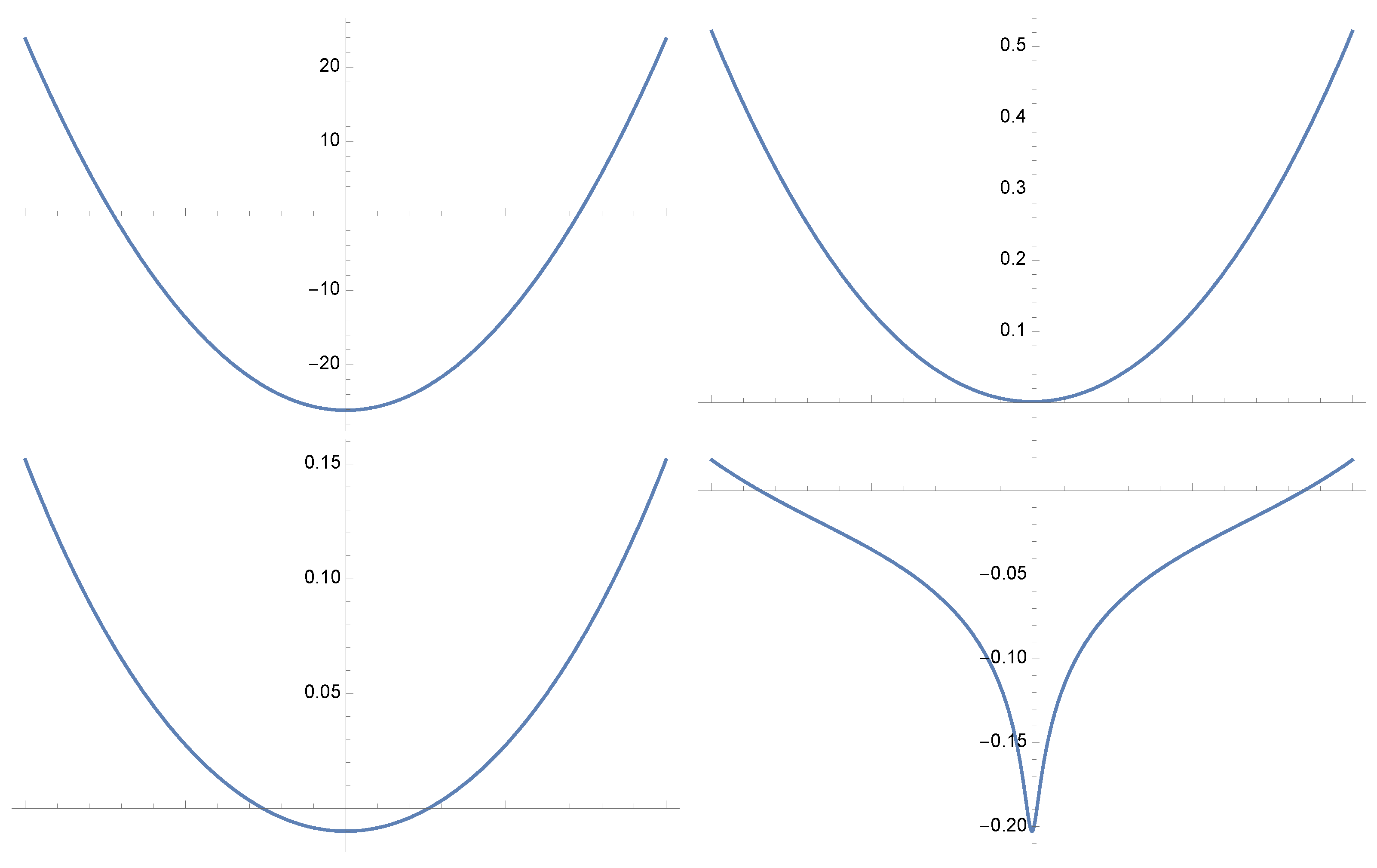
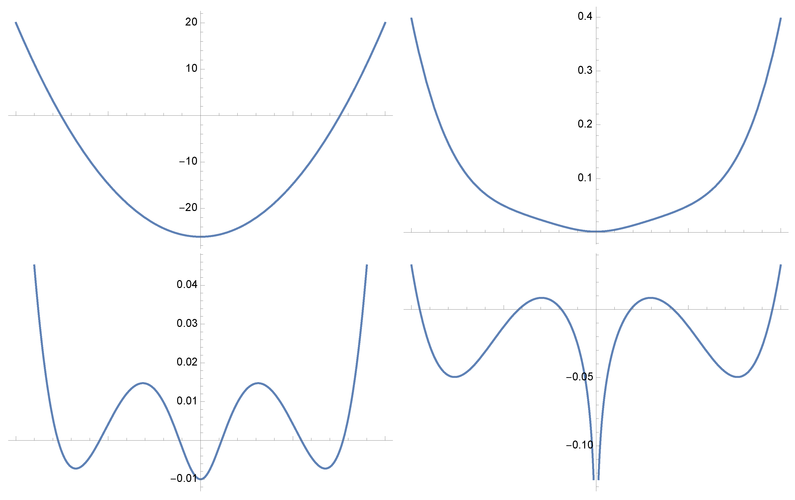
However, it is worth noting at this stage. While the relation between the mass parameter m and the physical mass $m_{phys}$ is quite cumbersome and involves curvature corrections, we may still wonder what happens in the $m\to 0$ limit. By inspection of the one-loop potential, according to Figure 1 and Figure 2, it happens that in the aforementioned limit the minimum becomes an infinite negative cusp, and the potential becomes concave in any small neighborhood of the origin. This situation is not improved by the second order corrections and, perhaps, it could be interpreted as due to some instability for small m. However, we see from the above expression of the physical mass that $m\to 0$ corresponds to $m_{phys}^2\to -\infty$, which has to be excluded by physical reasons. It would be of interest to analyze the case $m_{phys}\to 0$ to investigate the possible effect of anomalies, but it requires a numerical investigation that is out of the aims of the present article.

3.3.3. The Physical Coupling

The physical coupling is determined by the equation

$$\begin{array}{cc}\hfill c_{phys}=& 2{\displaystyle \frac{d^{2}V}{d{\left({\varphi }^2\right)}^2}}\left(0\right)=c-{\displaystyle \frac{(N+8)c^2}{8\pi \nu }}\coth \left(\pi R\nu \right)+{\displaystyle \frac{(N+8)c^{2}R}{8}}\left({\coth }^2\left(\pi R\nu \right)-1\right)\hfill \\ \hfill & +{\displaystyle \frac{27c^{3}R}{32{\pi }^2\nu }}[-{\displaystyle \frac{1}{2}}\left({\coth }^2\left(\pi R\nu \right)-1\right)f^{\prime }\left(R\nu \right)+{\displaystyle \frac{1}{2}}\left(1+3{\coth }^2\left(\pi R\nu \right)\right)f^{\prime }\left(3R\nu \right)\hfill \\ \hfill & +\pi \left({\coth }^2\left(\pi R\nu \right)-1\right)\coth \left(\pi R\nu \right)\left(f\left(R\nu \right)-f\left(3R\nu \right)\right)]\hfill \\ \hfill & +{\displaystyle \frac{(N-1)c^{3}R}{32{\pi }^2\nu }}[-{\displaystyle \frac{1}{2}}\left({\coth }^2\left(\pi R\nu \right)-1\right)f^{\prime }\left(R\nu \right)+{\displaystyle \frac{5}{2}}\left(1+3{\coth }^2\left(\pi R\nu \right)\right)f^{\prime }\left(3R\nu \right)\hfill \\ \hfill & +5\pi \left({\coth }^2\left(\pi R\nu \right)-1\right)\coth \left(\pi R\nu \right)\left(f\left(R\nu \right)-f\left(3R\nu \right)\right)].\hfill \end{array}$$

(96)

Again, we see that the relation between the coupling parameter c and the physical coupling is quite cumbersome. In order to get a better control of the physics, it is helpful to look at the flat limit.

3.4. Flat Limit

To take the flat limit, we consider $m\ge {\displaystyle \frac{1}{R}}$, which amounts to $mR\ge 1$. Noticing that ${\nu }_{jR}$ grows like R and dropping terms that in $V\left(\phi \right):={\displaystyle \frac{V\left({\phi }_R\right)}{R^3}}$ decrease exponentially or faster than ${\displaystyle \frac{1}{R^2}}$, we get

$$\begin{array}{cc}\hfill V\left(\phi \right)=& K_0+{\displaystyle \frac{m^2}{2}}{\phi }^2+{\displaystyle \frac{c}{4}}{\phi }^4-{\displaystyle \frac{{\nu }_0^3}{12\pi }}-{\displaystyle \frac{(N-1){\nu }_1^3}{12\pi }}+{\displaystyle \frac{c}{64{\pi }^2}}\left(3{\nu }_0^2+2(N-1){\nu }_0{\nu }_1+(N^2-1){\nu }_1^2\right)\hfill \\ \hfill & +{\displaystyle \frac{3c^2{\phi }^2}{32{\pi }^2}}\left(\log {\displaystyle \frac{1+9R^2{\nu }_0^2}{4}}-{\displaystyle \frac{4}{3}}{\displaystyle \frac{1}{1+9R^2{\nu }_0^2}}\right)\hfill \\ \hfill & +{\displaystyle \frac{c^2(N-1){\phi }^2}{32{\pi }^2}}\left(\log {\displaystyle \frac{1+R^2{({\nu }_0+2{\nu }_1)}^2}{4}}-{\displaystyle \frac{4}{3}}{\displaystyle \frac{1}{1+R^2{({\nu }_R+2{\nu }_1)}^2}}\right)+O\left(R^{-4}\right)\hfill \\ \hfill =& K_0+{\displaystyle \frac{m^2}{2}}{\phi }^2+{\displaystyle \frac{c}{4}}{\phi }^4-{\displaystyle \frac{{\nu }_0^3}{12\pi }}-{\displaystyle \frac{(N-1){\nu }_1^3}{12\pi }}+{\displaystyle \frac{c}{64{\pi }^2}}\left(3{\nu }_0^2+2(N-1){\nu }_0{\nu }_1+(N^2-1){\nu }_1^2\right)\hfill \\ \hfill & +{\displaystyle \frac{3c^2{\phi }^2}{32{\pi }^2}}\left(\log {\displaystyle \frac{27{\nu }_0^2}{2\mathcal{R}}}-{\displaystyle \frac{\mathcal{R}}{162{\nu }_0^2}}\right)+{\displaystyle \frac{c^2(N-1){\phi }^2}{32{\pi }^2}}\left(\log {\displaystyle \frac{3{({\nu }_0+2{\nu }_1)}^2}{2\mathcal{R}}}-{\displaystyle \frac{\mathcal{R}}{18{({\nu }_R+2{\nu }_1)}^2}}\right)\hfill \\ \hfill & +O\left(R^{-4}\right)\hfill \\ \hfill =& K_0+{\displaystyle \frac{m^2}{2}}{\phi }^2+{\displaystyle \frac{c}{4}}{\phi }^4-{\displaystyle \frac{M_0^3}{12\pi }}\left(1-{\displaystyle \frac{\mathcal{R}}{4M_0^2}}\right)-{\displaystyle \frac{(N-1)M_1^3}{12\pi }}\left(1-{\displaystyle \frac{\mathcal{R}}{4M_1^2}}\right)\hfill \\ \hfill & +{\displaystyle \frac{c}{64{\pi }^2}}\left(3M_0^2+2(N-1)M_0{M}_1+(N^2-1)M_1^2-{\displaystyle \frac{(N^2+2)M_0{M}_1+(N-1)(M_0^2+M_1^2)}{6}}\mathcal{R}\right)\hfill \\ \hfill & +{\displaystyle \frac{3c^2{\phi }^2}{32{\pi }^2}}\left(\log {\displaystyle \frac{27M_0^2}{2\mathcal{R}}}-{\displaystyle \frac{14\mathcal{R}}{81M_0^2}}\right)+{\displaystyle \frac{c^2(N-1){\phi }^2}{32{\pi }^2}}(\log {\displaystyle \frac{3{(M_0+2M_1)}^2}{2\mathcal{R}}}\hfill \\ \hfill & -{\displaystyle \frac{(3M_0^2+3M_1^2+8M_0{M}_1)}{3M_0{M}_1{(M_0+2M_1)}^2}}\mathcal{R})+O\left({\mathcal{R}}^2\right).\hfill \end{array}$$

(97)

It is clear that in the limit $\mathcal{R}=0$, this reproduces the two-loop effective potential with $N=1$, computed in [24], after the logarithmically divergent terms are absorbed in the renormalization of the mass. Indeed, in this approximation, the mass relation takes the form

$$m_{phys}^2=m^2-(N+2){\displaystyle \frac{c\nu }{4\pi }}+{\displaystyle \frac{{(N+2)}^2{c}^2}{32{\pi }^2}}+{\displaystyle \frac{(N+2)c^2}{16{\pi }^2}}\left(\log {\displaystyle \frac{27m^2}{2\mathcal{R}}}-{\displaystyle \frac{14}{81}}{\displaystyle \frac{\mathcal{R}}{m^2}}\right)+O\left({\mathcal{R}}^2\right).$$

(98)

Here we clearly see the physical meaning of the contributions: the first three terms determine the physical kinetic mass; the very last term gives the radiative correction to the $\xi$ parameter in the contribution ${\displaystyle \frac{1}{2}}\xi \mathcal{R}{\phi }^2$ (which, for simplicity, we initially assumed to be zero, but it could be equally included in $m^2$); the remaining logarithmic term looks like a Lamb-shift-like correction to the mass, essential for giving the correct flat limit.

As for the coupling constant, we get

$$c_{phys}=c-{\displaystyle \frac{(N+8)c^2}{8\pi \nu }}+{\displaystyle \frac{(5N+22)c^3}{72{\pi }^2{\nu }^2}}\left(1+{\displaystyle \frac{5}{54{\nu }^2}}\mathcal{R}\right)+O\left({\mathcal{R}}^2\right).$$

(99)

3.5. $\beta$-Function and Anomalous Mass Dimension

In order to compute the anomalous mass dimension, recall that the energy scaling must be restored by replacing the coupling c with $c{\mu }^{3-d}$, where $\mu ={\displaystyle \frac{\mathcal{E}}{{\mathcal{E}}_0}}$ is an adimensional energy scaling parameter, so that the renormalization of the mass is

$$\begin{array}{c}\hfill \delta m_0^2:={\displaystyle \frac{c^2{\mu }^{2(3-d)}(N+2)}{16{\pi }^2}}\left({\displaystyle \frac{1}{(d-3)}}-(1-\gamma +\log \left(\pi \right))\right).\end{array}$$

(100)

Therefore, the anomalous mass dimension is (for m, the renormalized mass)

$$\begin{array}{c}\hfill {\gamma }_m={\displaystyle \frac{\mu }{m}}{\partial }_{\mu }m=-{\displaystyle \frac{N+2}{16{\pi }^2}}{\displaystyle \frac{c^2}{m^2}}.\end{array}$$

(101)

It is also convenient to introduce the dimensionless coupling constant g defined by $c=mg$. It follows that the corresponding $\beta$-function is

$$\begin{array}{c}\hfill {\beta }_g={\displaystyle \frac{N+2}{16{\pi }^2}}{\displaystyle \frac{c^3}{m^2}}={\displaystyle \frac{N+2}{16{\pi }^2}}m{g}^3.\end{array}$$

(102)

These formulas coincide with the ones in the flat case [5].

4. Anti-de Sitter Effective Potentials

We compute the two-loop effective potential for the analogous model on AdS 3-dimensional spacetime; see [16] for field quantization on AdS. In this case, in place of the dimensional regularization, we will use point-splitting regularization.

4.1. The One-Loop Case

The d-dimensional real AdS spacetime with radius $R>0$ may be visualized as the manifold

$$\begin{array}{c}\hfill Ad{S}_d=\{x\in {\mathbf{R}}^{d+1}:x^2=x·x=R^2\}\end{array}$$

(103)

where the scalar product $x·x$ is intended in the sense of the ambient space ${\mathbf{R}}^{d+1}$ with two timelike directions and mostly minus metrics, as follows:

$$\begin{array}{c}\hfill x·y=x^0{y}^0-x^1{y}^1-\dots -x^{d-1}{y}^{d-1}+x^d{y}^d.\end{array}$$

(104)

The complexification of the AdS manifold is defined analogously

$$Ad{S}_d^{\left(c\right)}=\{z=x+iy\in {\mathbf{C}}^{d+1}:z^2=R^2\};$$

(105)

$z\in Ad{S}^{\left(c\right)}$ if and only if $x^2-y^2=R^2$ and $x·y=0$, i.e., the real and imaginary parts of z are orthogonal w.r.t. the scalar product in the ambient space.

The maximally analytic two-point function has the following expression of a massive scalar field (which is in general well-defined only on the universal covering of the AdS manifold)

$$\begin{array}{cc}\hfill & W_{\nu }^{\left(AdS\right)}(z_1,z_2)={\displaystyle \frac{1}{{\left(2\pi \right)}^{\frac{d}{2}}}}{({\zeta }^2-1)}^{-{\displaystyle \frac{d-2}{4}}}{e}^{-i\pi {\displaystyle \frac{d-2}{2}}}{Q}_{-{\displaystyle \frac{1}{2}}+\nu }^{{\displaystyle \frac{d-2}{2}}}\left(\zeta \right)=\hfill \end{array}$$

(106)

$$\begin{array}{c}\hfill ={\displaystyle \frac{\mathrm{\Gamma }\left(\frac{d-1}{2}+\nu \right)}{2{\pi }^{\frac{d-1}{2}}{\left(2\zeta \right)}^{\frac{d-1}{2}+\nu }\mathrm{\Gamma }(\nu +1)}}{}_{2}F_1\left({\displaystyle \frac{d-1}{4}}+{\displaystyle \frac{\nu }{2}},{\displaystyle \frac{d+1}{4}}+{\displaystyle \frac{\nu }{2}};\nu +1;{\displaystyle \frac{1}{{\zeta }^2}}\right)\end{array}$$

(107)

where

$$\zeta ={\displaystyle \frac{z_1·z_2}{R^2}}.$$

(108)

The Schwinger function (otherwise called the Euclidean propagator) is the restriction of the maximally analytic two-point function to the Euclidean Lobachevsky manifold. Choosing the points in Equation (106) as follows

$$\begin{array}{cc}\hfill & z_0=\left(1,0,\dots 0,0\right),z(u,\omega )=\left(u,{\omega }^1\sqrt{u^2-1},\dots ,{\omega }^{d-1}\sqrt{u^2-1},i{\omega }^d\sqrt{u^2-1}\right),u>1\hfill \end{array}$$

(109)

so that $\zeta =z_0·z(u,\omega )=u>1$, we write the propagator as

$$G_{\nu }^{\left(AdS\right)d}(z_0·z(u,\omega ))=G_{\nu }^{\left(AdS\right)d}\left(u\right)=G_{\nu }^d\left(u\right)=w_{\nu }\left(u\right)={\displaystyle \frac{e^{-i\pi \frac{d-2}{2}}}{{\left(2\pi \right)}^{\frac{d}{2}}}}{(u^2-1)}^{-{\displaystyle \frac{d-2}{4}}}{Q}_{-{\displaystyle \frac{1}{2}}+\nu }^{{\displaystyle \frac{d-2}{2}}}\left(u\right).$$

(110)

where the various parameters are related as follows:

$$m^2={\nu }^2-{\displaystyle \frac{{(d-1)}^2}{4}}.$$

(111)

The tadpole is computed from a maximally analytic two-point function by taking the limit $z_1·z_2\to 1$ in the above formula and, as before, it is finite for $d<2$:

$$T_d\left(\nu \right)={\displaystyle \frac{2^{-d}{\pi }^{-d/2}\mathrm{\Gamma }\left(1-\frac{d}{2}\right)\mathrm{\Gamma }\left(\frac{d-1}{2}+\nu \right)}{\mathrm{\Gamma }\left(\frac{3-d}{2}+\nu \right)}}$$

(112)

The meromorphic continuation of this formula provides a dimension-regularized integral representation of the 1-loop correction to the bare potential:

$$\begin{array}{c}\hfill V_0\left({\phi }_R\right)=2^{-d}{\pi }^{-d/2}\mathrm{\Gamma }\left(1-{\displaystyle \frac{d}{2}}\right){\int }^{\nu \left({\phi }_R\right)}{\displaystyle \frac{\mathrm{\Gamma }\left(\frac{d-1}{2}+x\right)}{\mathrm{\Gamma }\left(\frac{3-d}{2}+x\right)}}xdx\end{array}$$

(113)

where

$$\nu \left({\phi }_R\right)=\pm {\left(m_R^2+3c_R{\phi }_R^2+{\displaystyle \frac{{(d-1)}^2}{4}}\right)}^{{\displaystyle \frac{1}{2}}},\nu >-1.$$

(114)

The restriction $\nu >-1$ expresses the famous Breitenlohner and Freedman bound [35,36]. In dimensional regularization, the above formula directly gives the 1-loop correction to the effective potential in odd dimensions, much simpler than in de Sitter case; for instance, at $d=1$ and $d=3$

$$T_1\left(\nu \right)={\displaystyle \frac{1}{2\nu }},T_3\left(\nu \right)=-{\displaystyle \frac{\nu }{4\pi }}$$

(115)

so that

$$\begin{array}{ccc}& & V_0^{\left(1\right)}\left({\phi }_R\right)={\displaystyle \frac{1}{2}}\left(\sqrt{m_R^2+3c_R{\phi }_R^2}-m\right)\hfill \end{array}$$

(116)

$$\begin{array}{ccc}& & V_0^{\left(3\right)}\left({\phi }_R\right)={\displaystyle \frac{{\left(m_R^2+1\right)}^{3/2}-{\left(m_R^2+3c_R{\phi }_R^2+1\right)}^{3/2}}{12\pi }}.\hfill \end{array}$$

(117)

This is the flat space result! While this exact coincidence happens only in $d=1$ and $d=3$ (with a constant shift) it remains essentially verified in any odd dimension in the sense that when $d=2n+1$, the dominant term computed with the help of Equation (113) is identical to the flat space result (25).

In even dimensions the result is more complicated; for $d=2$ it reproduces the results in [37].

4.2. Two-Loop at $d=3$

We need to compute the banana diagram with three independent masses [23]. The n-loop banana integral on the Lobachevsky Euclidean manifold with $n+1$ edges and two vertices:

$$\begin{array}{c}\hfill I_{n+1}({\nu }_1,\dots ,{\nu }_{n+1},d)={\int }_{H_d}{G}_{{\nu }_1}^d(x·z)G_{{\nu }_2}^d(x·z)\dots G_{{\nu }_{n+1}}^d(x·z)\sqrt{g\left(z\right)}dz,\end{array}$$

(118)

where y varies on $H_d$ and x is a fixed reference point. The above definition has to be intended as a regularization of an expression that in general is divergent. Using the coordinates (109) with $u=\mathrm{ch}v$ and integrating over the angles (118) reduces to

$$\begin{array}{c}\hfill I_{n+1}({\nu }_1,\dots ,{\nu }_{n+1},d)={\displaystyle \frac{2{\pi }^{\frac{d}{2}}}{\mathrm{\Gamma }\left(\frac{d}{2}\right)}}{\int }_0^{\infty }{G}_{{\nu }_1}^d\left(\mathrm{ch}v\right)G_{{\nu }_2}^d\left(\mathrm{ch}v\right)\dots G_{{\nu }_{n+1}}^d\left(\mathrm{ch}v\right){\left(\mathrm{sh}v\right)}^{d-1}dv.\end{array}$$

(119)

We want to compute the two-loop diagram at $d=3$.

$$\begin{array}{c}\hfill I_3({\nu }_1,{\nu }_2,{\nu }_3,d)=4\pi {\int }_0^{\infty }{G}_{{\nu }_1}^3\left(\mathrm{ch}v\right)G_{{\nu }_2}^3\left(\mathrm{ch}v\right)G_{{\nu }_3}^3\left(\mathrm{ch}v\right){\left(\mathrm{sh}v\right)}^{2}dv.\end{array}$$

(120)

Here the propagator reduces to an elementary function: [28] (Equation (12), p. 150):

$$\begin{array}{cc}\hfill & G_{\nu }^3\left(\mathrm{ch}v\right)={\displaystyle \frac{e^{-\frac{i\pi }{2}}{Q}_{\nu -\frac{1}{2}}^{\frac{1}{2}}\left(\mathrm{ch}v\right)}{2\pi \sqrt{2\pi \mathrm{sh}v}}}={\displaystyle \frac{e^{-\nu v}}{4\pi \mathrm{sh}v}}.\hfill \end{array}$$

(121)

Notice that for each choice of mass one can take two values of $\nu$, but, for negative $\nu$, only $\nu >-1$ gives a good behaviour at infinity, confirming to the Breitenlohner–Freedman (BF) analysis [35,36]. Indeed, for large v, we see that G goes like ${\displaystyle \frac{1}{2\pi }}{u}^{-\mathrm{\Delta }}$, where $\mathrm{\Delta }={\displaystyle \frac{d-1}{2}}+\nu$ is the conformal weight of the dual theory. The choice of the sign of $\nu$ thus determines a quantum theory dual to a different conformal field theory. For the negative $\nu$, however, the resulting quantum field theory is unitary only for $-1<\nu <0$.

The bubble with two independent mass parameters ${\nu }_1$ and ${\nu }_2$ is readily decomposed into its Källén–Lehmann series by an elementary manipulation:

$$G_{{\nu }_1}^3\left(\mathrm{ch}v\right)G_{{\nu }_2}^3\left(\mathrm{ch}v\right)={\displaystyle \frac{e^{-({\nu }_1+{\nu }_2)v}}{16{\pi }^2{\mathrm{sh}}^{2}v}}={\displaystyle \sum _{k=0}^{\infty }}{\displaystyle \frac{e^{-({\nu }_1+{\nu }_2+1+2k)v}}{8{\pi }^2\mathrm{sh}v}}={\displaystyle \frac{1}{2\pi }}{\displaystyle \sum _{k=0}^{\infty }}{G}_{2k+1+{\nu }_1+{\nu }_2}^3\left(\mathrm{ch}v\right).$$

(122)

so that

$$\begin{array}{c}\hfill I_{3,K}({\nu }_1,{\nu }_2,{\nu }_3,d)={\displaystyle \frac{1}{8{\pi }^2}}{\displaystyle \sum _{k=0}^{\infty }}{\int }_K^{\infty }{e}^{-({\nu }_1+{\nu }_2+{\nu }_3+1+2k)v}dv.\end{array}$$

(123)

In the last step we exchanged the integral and the series and put a UV cutoff in the integration domain. Notice that in the standard quantization, corresponding to positive ${\nu }_j$ and with no restriction to the masses, there are no problems of convergence at infinity. But for small masses, in the BF interval, one can choose $\nu <0$. In this case, the convergence of the integral requires

$${\nu }_1+{\nu }_2+{\nu }_3+1>0.$$

(124)

This condition strictly limits the values of $\phi$ such that the calculation of the effective potential makes sense.

The above expression is readily computed and provides the regularized 2-loop bubble:

$$\begin{array}{ccc}\hfill I_{3,K}({\nu }_1,{\nu }_2,{\nu }_3,d)& =& {\displaystyle \frac{e^{-K({\nu }_1+{\nu }_2+{\nu }_3+1)}{}_{2}F_1\left(1,\frac{{\nu }_1+{\nu }_2+{\nu }_3+1}{2};\frac{{\nu }_1+{\nu }_2+{\nu }_3+3}{2};e^{-2K}\right)}{8{\pi }^2({\nu }_1+{\nu }_2+{\nu }_3+1)}}\hfill \\ & \simeq & -{\displaystyle \frac{1}{16{\pi }^2}}\psi \left({\displaystyle \frac{{\nu }_1+{\nu }_2+{\nu }_3+1}{2}}\right)-{\displaystyle \frac{\log \left(2K\right)+\gamma }{16{\pi }^2}}.\hfill \end{array}$$

(125)

This is essentially the point-splitting renormalization scheme. In order to renormalize the theory up to two-loops, we need to work in the same renormalization scheme at one-loop. In the point-splitting renormalization scheme, with point separation K, the tadpole in $d=3$ is

$$\begin{array}{c}\hfill T_3\left(\nu \right)=G_{\nu }^3\left(\mathrm{ch}K\right)={\displaystyle \frac{e^{-\nu K}}{4\pi \mathrm{sh}K}}\simeq {\displaystyle \frac{1}{4\pi K}}-{\displaystyle \frac{\nu }{4\pi }}.\end{array}$$

(126)

If $M\left({\phi }_R\right)$ is the field-dependent effective mass and $\nu \left({\phi }_R\right)=\sqrt{M{\left({\phi }_R\right)}^2+1}$, the one-loop contribution to the effective potential is therefore

$$\begin{array}{c}\hfill V_{1\mathrm{loop}}^{\left(3\right)}\left({\phi }_R\right)={\displaystyle \frac{\nu {\left(0\right)}^3-\nu {\left({\phi }_R\right)}^3}{12\pi }}+{\displaystyle \frac{M{\left({\phi }_R\right)}^2-M{\left(0\right)}^2}{8\pi K}}.\end{array}$$

(127)

We are now ready to write the point-splitting regularized effective potential up to two loops:

$$\begin{array}{cc}\hfill V\left({\phi }_R\right)=& {\mathrm{\Lambda }}_0+{\displaystyle \frac{m_R^2}{2}}{\phi }_R^2+{\displaystyle \frac{c_R}{4}}{\phi }_R^4+ħ{\displaystyle \frac{N+2}{8\pi K}}{c}_R{\phi }_R^2+ħ{\displaystyle \frac{N{\left(m_R^2+1\right)}^{\frac{3}{2}}-{\nu }_0{\left({\phi }_R\right)}^3-(N-1){\nu }_1{\left({\phi }_R\right)}^3}{12\pi }}\hfill \\ \hfill & +{ħ}^2{\displaystyle \frac{c_R}{4}}[3{\left({\displaystyle \frac{1}{4\pi K}}-{\displaystyle \frac{{\nu }_0\left({\phi }_R\right)}{4\pi }}\right)}^2+2(N-1)\left({\displaystyle \frac{1}{4\pi K}}-{\displaystyle \frac{{\nu }_0\left({\phi }_R\right)}{4\pi }}\right)\left({\displaystyle \frac{1}{4\pi K}}-{\displaystyle \frac{{\nu }_1\left({\phi }_R\right)}{4\pi }}\right)\hfill \\ \hfill & +(N^2-1){\left({\displaystyle \frac{1}{4\pi K}}-{\displaystyle \frac{{\nu }_1\left({\phi }_R\right)}{4\pi }}\right)}^2]+{ħ}^2(N+2){\displaystyle \frac{c_R^2{\phi }_R^2}{16{\pi }^2}}(\log \left(2K\right)+\gamma )\hfill \\ \hfill & +{ħ}^2{\displaystyle \frac{c_R^2{\phi }_R^2}{16{\pi }^2}}\left(3\psi \left({\displaystyle \frac{3{\nu }_0\left({\phi }_R\right)+1}{2}}\right)+(N-1)\psi \left({\displaystyle \frac{{\nu }_0\left({\phi }_R\right)+2{\nu }_1\left({\phi }_R\right)+1}{2}}\right)\right)+O\left({ħ}^3\right),\hfill \end{array}$$

(128)

where we have restored ħ for practical purposes. We see that in this scheme the divergences appear in a bit more of a complicated way than in dimensional regularization. Like in the $dS$ case, we must divide $V_{2\mathrm{loop}}\left({\phi }_R\right)$ by $R^3$ and then define the renormalized parameters. In order to simplify the notations, we assume momentarily $R=1$, which will then be restored at the end. Next, we introduce the renormalized field ${\phi }_r$, mass $m_r$ and coupling constant $c_r$, so that

$$\begin{array}{c}\hfill {\phi }_R={\phi }_r\sqrt{Z_{\varphi }},m_R^2=m_r^2{\displaystyle \frac{Z_{m^2}}{Z_{\varphi }}},c_R=c{\displaystyle \frac{Z_c}{Z_{\varphi }^2}}.\end{array}$$

(129)

By setting (lfor $Z_{\varphi }$ we can take only $Z_{\varphi }^{\prime }$, since $Z_{\varphi }^{″}$ enters at the third order in ħ)

$$Z_a=1+ħZ_a^{\prime }+{ħ}^2{Z}_a^{″}+O\left({ħ}^3\right),$$

(130)

$${\mathrm{\Lambda }}_0=\mathrm{\Lambda }+ħ{\mathrm{\Lambda }}^{\prime }+{ħ}^2{\mathrm{\Lambda }}^{″},$$

(131)

replacing in (128), and expanding up to order ${ħ}^2$ (and finally setting $ħ=1$), we get from the renormalization conditions

$$\begin{array}{cc}\hfill V\left({\phi }_r\right)=& \mathrm{\Lambda }+{\displaystyle \frac{m_r^2}{2}}{\phi }_r^2+{\displaystyle \frac{c_r}{4}}{\phi }_r^4+{\displaystyle \frac{N{\left(m_r^2+1\right)}^{\frac{3}{2}}-{\nu }_0{\left({\phi }_r\right)}^3-(N-1){\nu }_1{\left({\phi }_r\right)}^3}{12\pi }}\hfill \\ \hfill & +{\displaystyle \frac{c_r}{64{\pi }^2}}\left[3{\nu }_0{\left({\phi }_r\right)}^2+2(N-1){\nu }_0\left({\phi }_r\right){\nu }_1\left({\phi }_r\right)+(N^2-1){\nu }_1{\left({\phi }_r\right)}^2\right]\hfill \\ \hfill & +{\displaystyle \frac{c_r^2{\phi }_r^2}{16{\pi }^2}}\left(3\psi \left({\displaystyle \frac{3{\nu }_0\left({\phi }_r\right)+1}{2}}\right)+(N-1)\psi \left({\displaystyle \frac{{\nu }_0\left({\phi }_r\right)+2{\nu }_1\left({\phi }_r\right)+1}{2}}\right)\right),\hfill \end{array}$$

(132)

and

$$Z_{\varphi }=Z_c=1,$$

(133)

$$Z_{m^2}^{\prime }=-{\displaystyle \frac{N+2}{4\pi K}}{\displaystyle \frac{c_r}{m_r^2}},Z_{m^2}^{″}=-{\displaystyle \frac{N+2}{8{\pi }^2}}{\displaystyle \frac{c_r^2}{m_r^2}}(\log \left(2K\right)+\gamma ),$$

(134)

$${\mathrm{\Lambda }}^{\prime }=0,{\mathrm{\Lambda }}^{″}={\displaystyle \frac{N(N+2)c_r}{32{\pi }^{2}K}}\left({\displaystyle \frac{1}{2K}}-{\left({\displaystyle \frac{1}{R^2}}+m_r^2\right)}^{{\displaystyle \frac{1}{2}}}\right),$$

(135)

where

$${\nu }_0\left({\phi }_r\right)=\sqrt{m_r^2+3c_r{\phi }_r^2+{\displaystyle \frac{1}{R^2}}},$$

(136)

$${\nu }_1\left({\phi }_r\right)=\sqrt{m_r^2+c_r{\phi }_r^2+{\displaystyle \frac{1}{R^2}}},$$

(137)

and we have restored R. Like in the de Sitter case, we see that we have only mass renormalization:

$$\begin{array}{c}\hfill m^2=m_r^2-{\displaystyle \frac{N+2}{4\pi K}}{c}_r-{\displaystyle \frac{N+2}{8{\pi }^2}}{c}_r^2(\log (2K/R)+\gamma ).\end{array}$$

(138)

Notice that the above formula for the potential is also valid in the BF region

$${\nu }_0\left({\phi }_r\right)=-\sqrt{m_r^2+3c_r{\phi }_r^2+{\displaystyle \frac{1}{R^2}}},$$

(139)

$${\nu }_1\left({\phi }_r\right)=-\sqrt{m_r^2+c_r{\phi }_r^2+{\displaystyle \frac{1}{R^2}}},$$

(140)

for which, however, accordingly with (124), we must require the condition

$$\begin{array}{c}\hfill 3{\nu }_0\left({\phi }_r\right)>-1\end{array}$$

(141)

to avoid the poles in the digamma functions $\psi$. Thus, the effective potential in the BF region looks to be just the analytic continuation in $\nu$ of the one in standard quantization, along the real axis, subject to the condition (124). However, of course, the two results are not related since they correspond to two different quantum field theories. Curiously, this bound is only manifest in the perturbative expansion of the effective potential from the two-loop order onward.

4.3. $\beta$-Function and Anomalous Mass Dimension

After recalling that the energy scale is given by $\mu =1/K$, we can absorb the local counterterms, which do not contribute to the anomalous dimension, in the regular part of the mass, and write

$$\begin{array}{c}\hfill m_{\left(reg\right)}^2=m_r^2+{\displaystyle \frac{N+2}{8{\pi }^2}}{c}_r^2(\log \left(2\mu R\right)+\gamma ).\end{array}$$

(142)

The mass anomalous dimension is therefore

$$\begin{array}{c}\hfill {\gamma }_m=-{\displaystyle \frac{N+2}{16{\pi }^2}}{\displaystyle \frac{c_r^2}{m_r^2}}.\end{array}$$

(143)

This is exactly the same result as in the flat case. It is also convenient to introduce a dimensionless coupling constant $g_r$ through the expression

$$\begin{array}{c}\hfill c_r=m_r{g}_r.\end{array}$$

(144)

The associated beta function is therefore

$$\begin{array}{c}\hfill {\beta }_g=-c_r{\gamma }_m={\displaystyle \frac{N+2}{16{\pi }^2}}{\displaystyle \frac{c_r^3}{m_r^2}}.\end{array}$$

(145)

Again, this is the same result as in the flat case. Nevertheless, we remark that, in both dS and AdS cases, what makes the difference is the relation among the renormalized parameters $m_r,g_r$ and the physical parameters $m_p,g_p$.

5. Conclusions

In this work we have derived the first systematic treatment of one-loop effective potentials for interacting scalar fields in curved spacetimes, with explicit results for maximally symmetric de Sitter and anti-de Sitter backgrounds. Our key results can be summarized as follows:

We determined a general formula (Equation (22)) for the one-loop effective potential in arbitrary curved geometries that satisfies the simple differential condition (8) for the propagator. Next, we have specified our formula to the de Sitter and anti-de Sitter maximally symmetric spaces. In particular, for de Sitter, we compute the effective potential for the scalar theory ${\phi }^4$ with symmetry $O\left(N\right)$ for any dimension, with an emphasis on dimensions $1,2,3,$ and 4. This is done in dimensional regularization. For the principal series, the potential is convex for a small interaction parameter as compared to the mass parameter. Convexity is lost for large values of the coupling constant. This is not surprising, since the perturbative approach is expected to become inefficient as the coupling increases. In principle, convexity could be recovered by including higher-order corrections or nonperturbative methods. A possible approach to recover convexity is proposed, for example, in [38]. However, that method requires infinite volume, while we are working on a sphere of finite volume. In dimension $d=3$, still in dimensional regularization, we have extended the calculations to two-loops, and computed the $\beta$-function and the anomalous mass dimension. The final expressions are identical to the ones for the flat case but with different relations between the renormalized parameters and the physical parameters. We also performed the flat limit $R\to \infty$, recovering the standard Minkowski results, confirming the construction’s consistency and enabling precision comparisons between curved/flat physics.

Next, we have computed the two-loop effective potential for the same model on $Ad{S}_3$. To illustrate the power of our methods in the configuration space, we worked with the point-splitting regularization. This resulted in a very simple calculation also at two-loops. The main difference is that non-logarithmic divergent terms appear already at one-loop. Since they are of local type, these do not contribute to the $\beta$-function and anomalous mass dimension, and we find once more the same expression as in the flat case. These results also extend to the Breitenlohner–Freedman region, with a lower bound on $\nu$ that is manifest only beyond one-loop.

These results have immediate implications across multiple frontiers. Our $d=4$ de Sitter effective potentials (Equation (59)) provide a reliable framework for Higgs stability and radiative symmetry breaking during inflation, where flat space approximations fail catastrophically. The $d=3$ results (Equations (90) and (132)) are directly applicable to critical phenomena modeled by QFTs on $S^3$ and $H^3$. These could be suitably analyzed by using non-perturbative functional renormalization group methods. These applications will be considered in future work.

References

1. Sher, M. Electroweak Higgs Potentials and Vacuum Stability. Phys. Rep. 1989, 179, 273–418. [Google Scholar] [CrossRef] [Scilit]
2. Branchina, V.; Faivre, H.; Pangon, V. Effective potential and vacuum stability. J. Phys. G 2009, 36, 015006. [Google Scholar] [CrossRef] [Scilit]
3. Coleman, S.; Weinberg, E. Radiative corrections as the origin of spontaneous symmetry breaking. Phys. Rev. 1973, D7, 1888. [Google Scholar] [CrossRef] [Scilit]
4. Guida, R.; Zinn-Justin, J. Critical exponents of the N vector model. J. Phys. A 1998, 31, 8103–8121. [Google Scholar] [CrossRef] [Scilit]
5. Kleinert, H.; Schulte-Frohlinde, V. Critical Properties of Φ4 Theories; World Scientific: Berlin, Germany, 2001. [Google Scholar]
6. Zinn-Justin, J. Quantum field theory and critical phenomena. Int. Ser. Monogr. Phys. 2002, 113, 1–1054. [Google Scholar]
7. Isidori, G.; Ridolfi, G.; Strumia, A. On the metastability of the standard model vacuum. Nucl. Phys. B 2001, 609, 387–409. [Google Scholar] [CrossRef] [Scilit]
8. Fairbairn, M.; Grothaus, P.; Hogan, R. The Problem with False Vacuum Higgs Inflation. J. Cosmol. Astropart. Phys. 2014, 6, 39. [Google Scholar] [CrossRef] [Scilit]
9. Anderson, P.R.; Holman, R. Effective potential for the O(N)-symmetric model in static homogeneous spacetimes. Phys. Rev. D 1986, 34, 2277. [Google Scholar] [CrossRef] [Scilit]
10. Elizalde, E.; Kirsten, K.; Odintsov, S.D. Effective Lagrangian and the back-reaction problem in a self-interacting O(N) scalar theory in curved spacetime. Phys. Rev. D 1994, 50, 5137. [Google Scholar] [CrossRef] [Scilit]
11. Buchbinder, I.L.; Odintsov, S.D.; Shapiro, I.L. Effective Action in Quantum Gravity; IOP: Bristol, UK, 1992. [Google Scholar]
12. Guth, A.H. Inflationary universe: A possible solution to the horizon and flatness problems. Phys. Rev. D 1981, 23, 347–356. [Google Scholar] [CrossRef] [Scilit]
13. Witten, E. Anti de Sitter space and Holography. Adv. Theor. Math. Phys. 1998, 2, 253–291. [Google Scholar] [CrossRef] [Scilit]
14. Bros, J.; Moschella, U.; Gazeau, J.P. Quantum field theory in the de Sitter universe. Phys. Rev. Lett. 1994, 73, 1746–1749. [Google Scholar] [CrossRef] [Scilit]
15. Bros, J.; Moschella, U. Two point functions and quantum fields in de Sitter universe. Rev. Math. Phys. 1996, 8, 327–392. [Google Scholar] [CrossRef] [Scilit]
16. Bros, J.; Epstein, H.; Moschella, U. Towards a general theory of quantized fields on the anti-de Sitter space-time. Commun. Math. Phys. 2002, 231, 481–528. [Google Scholar] [CrossRef] [Scilit]
17. Moschella, U. Anti-de Sitter, plane waves and quantum field theory. Phys. Lett. B 2025, 871, 139979. [Google Scholar] [CrossRef] [Scilit]
18. Lee, S.Y.; Sciaccaluga, A.M. Evaluation of Higher Order Effective Potentials with Dimensional Regularization. Nucl. Phys. B 1975, 96, 435–444. [Google Scholar] [CrossRef] [Scilit]
19. Prokopec, T.; Reska, P. Scalar cosmological perturbations from inflationary black holes. J. Cosmol. Astropart. Phys. 2011, 3, 50. [Google Scholar] [CrossRef] [Scilit]
20. Haba, Z. Euclidean scalar Green functions near the black hole and black brane horizons. Class. Quant. Grav. 2009, 26, 075022. [Google Scholar] [CrossRef] [Scilit]
21. Cacciatori, S.L.; Epstein, H.; Moschella, U. Loops in de Sitter space. J. High Energy Phys. 2024, 7, 182. [Google Scholar] [CrossRef] [Scilit]
22. Bros, J.; Epstein, H.; Gaudin, M.; Moschella, U.; Pasquier, V. Anti de Sitter quantum field theory and a new class of hypergeometric identities. Commun. Math. Phys. 2012, 309, 255–291. [Google Scholar] [CrossRef] [Scilit]
23. Cacciatori, S.L.; Epstein, H.; Moschella, U. Loops in anti de Sitter space. J. High Energy Phys. 2024, 8, 109. [Google Scholar] [CrossRef] [Scilit]
24. Rajantie, A.K. Feynman diagrams to three loops in three-dimensional field theory. Nucl. Phys. B 1996, 480, 729–752, Erratum in Nucl. Phys. B 1998, 51, 761–762. [Google Scholar] [CrossRef] [Scilit]
25. Inami, T.; Ooguri, H. One Loop Effective Potential in Anti-de Sitter Space. Prog. Theor. Phys. 1985, 73, 1051. [Google Scholar] [CrossRef] [Scilit]
26. Bros, J.; Epstein, H.; Moschella, U. Scalar tachyons in the de Sitter universe. Lett. Math. Phys. 2010, 93, 203–211. [Google Scholar] [CrossRef] [Scilit]
27. Epstein, H.; Moschella, U. de Sitter tachyons and related topics. Commun. Math. Phys. 2015, 336, 381–430. [Google Scholar] [CrossRef] [Scilit]
28. Erdélyi, A. (Ed.) The Bateman Project: Higher Transcendental Functions; McGraw-Hill Book Company: New York, NY, USA, 1953; Volume I. [Google Scholar]
29. Weinberg the Quantum Theory of Fields; Cambridge University Press: Cambridge, UK, 1996; Volume II.
30. Vicente García-Consuegra, L.; Rajantie, A. Scalar field effective potentials in de Sitter spacetime. arXiv 2025, arXiv:2511.23076. [Google Scholar] [CrossRef] [Scilit]
31. Fujimoto, Y.; Ishihara, H. One Loop Effective Potential for Lambda Φ4 Theory in De Sitter Space. Phys. Lett. B 1987, 191, 46–50. [Google Scholar] [CrossRef] [Scilit]
32. Shore, G.M. Radiatively Induced Spontaneous Symmetry Breaking and Phase Transitions in Curved Space-Time. Ann. Phys. 1980, 128, 376. [Google Scholar] [CrossRef] [Scilit]
33. Esposito, G.; Miele, G.; Rosa, L. One loop effective potential for SO(10) GUT theories in de Sitter space. Class. Quant. Grav. 1994, 11, 2031–2044. [Google Scholar] [CrossRef] [Scilit]
34. Whittaker, E.T.; Watson, G.N. A Course of Modern Analysis, 5th ed.; Moll, V.H., Ed.; Cambridge University Press: Cambridge, UK, 2021. [Google Scholar]
35. Breitenlohner, P.; Freedman, D.Z. Stability in Gauged Extended Supergravity. Ann. Phys. 1982, 144, 249. [Google Scholar] [CrossRef] [Scilit]
36. Bertola, M.; Bros, J.; Gorini, V.; Moschella, U.; Schaeffer, R. Decomposing quantum fields on branes. Nucl. Phys. B 2000, 581, 575–603. [Google Scholar] [CrossRef] [Scilit]
37. Sakai, N.; Tanii, Y. Effective Potential in Two-dimensional Anti-de Sitter Space. Nucl. Phys. B 1985, 255, 401. [Google Scholar] [CrossRef] [Scilit]
38. Wiedemann, U.A. Non-differentiability of the effective potential. Nucl. Phys. B 1993, 406, 808–822. [Google Scholar] [CrossRef] [Scilit]
Figure 1. One-loop effective potential in the de Sitter d = 3 case. The bare coupling constant is c R = 0.1 . The masses from left to right: principal series m R = 10 , limit case m R = 1 , complementary series m R = 0.5 and m R = 0.001 .
Symmetry 18 00801 g001
Figure 2. One-loop effective potential in the de Sitter d = 3 case. The bare coupling constant is c R = 4 . The masses from left to right: principal series m R = 10 , limit case m R = 1 , complementary series m R = 0.5 and m R = 0.001 . One observes the curious behavior of the complementary series. Further analysis is needed with the renormalization group.
Symmetry 18 00801 g002
Disclaimer/Publisher’s Note: The statements, opinions and data contained in all publications are solely those of the individual author(s) and contributor(s) and not of MDPI and/or the editor(s). MDPI and/or the editor(s) disclaim responsibility for any injury to people or property resulting from any ideas, methods, instructions or products referred to in the content.