Statistical Inference for Drift Parameters in Gaussian White Noise Models Driven by Caputo Fractional Dynamics Under Discrete Observation Schemes

Abstract

This paper develops a rigorous inferential framework for a class of Gaussian stochastic processes driven by white noise with constant drift, whose temporal evolution is governed by a Caputo fractional derivative of order ${\displaystyle \alpha \in (1/2,1)}$. The model belongs to the family of fractional Volterra processes, where memory is generated by the dynamics themselves rather than by correlated noise. We derive explicit analytical expressions for the mean, variance, and covariance structure of the solution, thereby characterizing in a precise manner how the fractional order ${\displaystyle \alpha }$ governs both variance growth and the strength of temporal dependence. In particular, the process exhibits correlated increments and a power-law variance scaling of order ${\displaystyle t^{2\alpha -1}}$, highlighting the dual role of ${\displaystyle \alpha }$ as a regularity and memory parameter. Building on this structural analysis, we address the statistical problem of estimating the parameter vector ${\displaystyle (\mu ,\sigma ,\alpha )}$ from discrete-time observations. Two complementary procedures are proposed for the estimation of the fractional order: a variance-growth method based on log–log regression of empirical variances, and a wavelet-based estimator exploiting multi-scale scaling properties of the process. For the drift and diffusion parameters ${\displaystyle (\mu ,\sigma )}$, we construct explicit Gaussian pseudo-maximum likelihood estimators derived from the Volterra covariance structure of the increment process. We establish unbiasedness, ${\displaystyle L^2}$-convergence, strong consistency, and asymptotic normality for all estimators. Furthermore, we derive Berry–Esseen type bounds that quantify the rate of convergence toward the Gaussian law, providing sharp distributional approximations in a genuinely fractional and non-Markovian setting. A Monte Carlo study is carried out, using high-resolution Volterra discretizations, large-scale simulation budgets, covariance-structured linear algebra, and multi-scale diagnostic tools. The numerical experiments confirm the theoretical convergence rates, demonstrate the finite-sample reliability of the estimators, and illustrate the sensitivity of the process dynamics to the fractional order ${\displaystyle \alpha }$: smaller values of ${\displaystyle \alpha }$ produce stronger memory effects and higher variability, while values closer to one lead to smoother and more stable trajectories. The proposed methodology unifies statistical inference for long-memory Gaussian processes with fractional differential stochastic dynamics, offering a coherent analytical and computational framework applicable in areas such as quantitative finance, anomalous diffusion in physics, hydrology, and engineering systems with hereditary effects.

1. Introduction

The mathematical theory of long-memory stochastic processes has become one of the most structurally refined areas of contemporary probability, propelled by a sustained feedback loop between advances in stochastic analysis and the repeated empirical appearance of persistent dependence in complex systems. Long-range dependence—mathematically expressed through hyperbolic decay of autocorrelation functions or, equivalently, by a spectral density that diverges at the origin—has been reported across an exceptionally broad scientific spectrum, spanning hydrology, geophysics, climatology, telecommunications, economics, finance, statistical physics, and biology, as well as more unconventional settings such as medicine, music, and large-scale network traffic (see, e.g., [1,2,3,4,5,6,7,8,9,10,11]). This ubiquity is not merely anecdotal: it has forced a methodological shift away from short-memory paradigms, positioning Gaussian long-memory processes as indispensable primitives for modeling temporal complexity.

Among these processes, fractional Brownian motion (fBM), introduced by Mandelbrot and Van Ness, occupies a canonical status. Its self-similarity, stationary increments, and covariance structure governed by the Hurst index ${\displaystyle H\in (0,1)}$ provide a uniquely tractable yet phenomenologically expressive framework—especially in the long-memory regime ${\displaystyle H>1/2}$. The systematic development of stochastic calculus with respect to fBM (see [12]) has enabled a broad range of theoretical and applied contributions. In financial econometrics, geometric fractional Brownian motion (gfBM) has been advocated as a parsimonious mechanism for persistent dependence in asset dynamics [13,14,15], while in geophysical and environmental sciences, fBM-type structures have proven effective in capturing long-term correlations in oceanographic and meteorological signals [16,17,18].

A natural refinement is sub-fractional Brownian motion (sub-fBM), which retains self-similarity but departs from stationarity of increments and exhibits a distinct covariance geometry. Its “intermediate” dependence behavior has repeatedly appeared as a better phenomenological compromise in applications where neither strictly short-memory nor strictly long-memory Gaussian models yield satisfactory fits. This point is conceptually important: Gaussian long-memory modeling is best viewed as a hierarchy of covariance geometries rather than a single paradigm, and inference must adapt to the particular way memory is encoded.

Inference under persistent dependence: what is known and what remains subtle. Despite the maturity of the modeling landscape, statistical inference for long-memory processes remains intrinsically delicate. The slow decay of correlations undermines many classical asymptotic arguments designed for weak dependence, while non-Markovianity obstructs direct likelihood constructions under discrete-time sampling. As a consequence, the estimation of drift, volatility, and memory parameters has served as a crucible for methodological innovation.

Malliavin calculus has become a central tool for deriving limit theorems and asymptotic normality for nonlinear functionals of Gaussian processes [19]. In parallel, Stein’s method has enabled quantitative distributional approximations—most notably Berry–Esseen bounds with explicit rates—for estimators arising in dependent Gaussian settings [20,21]. Quadratic and multipower variation methods have delivered robust nonparametric procedures that remain informative under mild misspecification [22], while wavelet-based and random-walk approximations have provided computationally efficient multiscale inference strategies. For sub-fBM, the works [23,24] demonstrated that Malliavin–Stein techniques can be fused to establish consistency and central limit theorems, and [25] proposed a unifying likelihood-based treatment across a broad class of Gaussian long-memory processes.

Collectively, these contributions make clear that rigorous inference in the presence of persistence requires a careful synthesis of Gaussian analysis, stochastic calculus, and asymptotic statistics. Yet there is a structural asymmetry in the literature: the bulk of results concern models in which long memory is carried by the driving noise (fractional Gaussian noise and its relatives). The equally natural—and in many applications more mechanistically faithful—scenario in which memory is carried by the dynamics themselves via fractional operators has not received a comparably systematic inferential treatment.

Emerging directions: mixed fractional models and fractional differential dynamics. Since 2019, a substantial effort has been devoted to mixed fractional models that superimpose Brownian and fractional Brownian components to encode short- and long-range dependence simultaneously. Such hybridization has proven empirically compelling and theoretically fertile. For example, ref. [26] developed consistent estimators for mixed fBM with drift, while [27] reported empirical robustness on Nordic stock markets. The analysis of gfBM in [28] leveraged bipower variation and least-squares ideas to obtain consistency without restrictive small-step constraints, and [29] established joint asymptotic normality for Gaussian processes with drift through Stein–Malliavin arguments. The work [30] pushed the asymptotic theory into the rough regime ${\displaystyle H\in (0,1/2)}$ for mixed fBM with trend, closing a technically significant gap in rough long-memory inference.

Running in parallel, and conceptually deeper, is the rise of fractional stochastic differential equations (FSDEs), where classical derivatives are replaced by fractional operators—most prominently of Caputo type—so that memory enters through the evolution law itself. This modeling choice is not cosmetic: it encodes hereditary effects through nonlocal temporal kernels, thereby coupling instantaneous Gaussian fluctuations with persistent history dependence. FSDEs now play a central role in the mathematical description of anomalous diffusion, viscoelasticity, turbulence, and transport in physics; hereditary dynamics in biology; long-memory volatility modeling in finance; and engineering systems with fading memory and control under uncertainty. Foundational analyses include [12,31,32,33], while fractional Ornstein–Uhlenbeck-type processes have been studied in depth in [34,35,36]. The modeling and analytic significance of Caputo derivatives as a mathematically coherent embodiment of temporal nonlocality is emphasized further in [37,38].

A structural gap: inference for Gaussian white-noise driven Caputo dynamics. Despite the breadth of this literature, a notable methodological gap persists. The statistical theory for FSDEs driven by Gaussian white noise—where memory is induced solely by the fractional derivative—remains comparatively fragmented. This setting differs sharply from fBM-driven models: dependence is generated by the Volterra kernel in the solution representation rather than by the covariance of the noise. Consequently, the increment structure is correlated in a kernel-driven manner, likelihood geometry is non-Markovian for reasons that are analytically distinct from fractional Gaussian noise, and identifiability regimes for the memory parameter differ.

In particular, the fractional order ${\displaystyle \alpha }$ in Caputo dynamics plays a dual role: it governs local variance-growth and global correlation strength simultaneously, acting as both a regularity and a memory exponent. From an inferential standpoint, this duality is precisely where standard long-memory tools are insufficient: one needs procedures that exploit scaling information without discarding the dependence structure, and one needs asymptotic theory that remains quantitative rather than merely qualitative. These considerations become even more pressing in modern data-rich contexts where scalable, robust, and uncertainty-aware inference is required. Recent attempts to incorporate neural and deep learning architectures into FSDE parameter estimation [39,40] underline the practical demand, but also highlight that theoretical guarantees in genuinely fractional and nonlocal settings are still scarce. Moreover, robustness under rough noise and perturbations—see, e.g., [41]—adds an additional layer of difficulty that further motivates mathematically explicit inference frameworks.

Motivation and contributions of the present work. The purpose of this paper is to provide a coherent and technically explicit inferential theory for a Gaussian white-noise model with drift governed by a Caputo fractional derivative, under discrete-time observation. Our contribution is to operationalize the Volterra structure of the solution into statistically tractable estimators and sharp asymptotic statements.

Concretely, we (i) derive explicit representations and closed-form expressions for the mean, variance, and covariance structure of the solution, isolating the precise way in which ${\displaystyle \alpha }$ reshapes dependence and scaling; (ii) construct complementary estimators for the full parameter vector ${\displaystyle (\alpha ,\mu ,{\sigma }^2)}$, combining variance-growth and wavelet-based procedures for ${\displaystyle \alpha }$ with Gaussian pseudo-maximum likelihood inference for ${\displaystyle (\mu ,{\sigma }^2)}$; and (iii) go beyond consistency and central limit theorems by establishing Berry–Esseen type bounds that quantify the accuracy of Gaussian approximations in finite samples.

By embedding Caputo-driven fractional dynamics within the quantitative inferential paradigm developed for Gaussian long-memory processes—yet adapting it to the distinctive kernel-induced dependence of white-noise driven FSDEs—the present work closes a structural gap between two strands of the literature that have largely evolved in parallel. We argue that this synthesis is not only technically nontrivial but conceptually clarifying: it reveals how memory generated by the dynamics (rather than by the noise) can be exploited for statistically efficient and uncertainty-aware inference, thereby providing a rigorous reference framework for applications in physics, finance, biology, and engineering where hereditary effects are intrinsic to the underlying mechanisms.

Organization of the Paper

The paper is organized as follows. In Section 2, we introduce the probabilistic and analytic framework. We first recall the Malliavin calculus tools that will be used for normal approximations and Berry–Esseen bounds, including Wiener chaoses, multiple Wiener–Itô integrals, contractions, and the Kolmogorov distance. We then review fractional calculus notions (Riemann–Liouville integrals/derivatives and the Caputo derivative), and we present the Caputo fractional stochastic differential equation driven by Gaussian white noise with drift. In the constant-coefficient case, we provide the Volterra representation of the solution as well as explicit expressions for the mean, variance and covariance structure, highlighting the correlation of increments. Section 3 is devoted to the estimation of the fractional differentiation order ${\displaystyle \alpha }$. We first develop a variance-growth estimator based on the power-law behavior ${\displaystyle \mathrm{Var}\left(X_t\right)\propto t^{2\alpha -1}}$ and a log–log linear regression built from independent trajectories observed at fixed design points. We then establish the main asymptotic properties of the resulting estimator, including unbiasedness, ${\displaystyle L^2}$–convergence, strong consistency, and asymptotic normality with an explicit asymptotic variance. Next, we propose a wavelet-based procedure for estimating ${\displaystyle \alpha }$, relying on the scaling of wavelet coefficients and vanishing moments, as a complementary and more robust alternative. In Section 4, we address the estimation of the drift and diffusion parameters ${\displaystyle \mu }$ and ${\displaystyle {\sigma }^2}$. Using a high-frequency discretization of the Volterra representation, we derive a Gaussian pseudo-likelihood for the increment vector and obtain explicit closed-form pseudo-maximum likelihood estimators. We then study their large-sample behavior: consistency, central limit theorems, and quantitative normal approximation results. In particular, we derive Berry–Esseen type bounds in Kolmogorov distance for the standardized volatility estimator. Section 5 presents a Monte Carlo study assessing the finite-sample performance of the proposed estimators for ${\displaystyle (\alpha ,\mu ,{\sigma }^2)}$ under various grid sizes and replication budgets. We report bias, RMSE, empirical standard deviations, and coverage probabilities of asymptotic confidence intervals, and we provide graphical diagnostics illustrating the effect of ${\displaystyle \alpha }$ on the trajectories and on estimator distributions. Finally, Section 7 concludes the paper and discusses perspectives and possible extensions. The proofs of the main theoretical results are gathered in Section 8, and a few additional technical lemmas and auxiliary calculations are provided in the Appendix A.

2. Gaussian White Noise with Drift and Caputo Fractional Derivative

2.1. Elements of Malliavin Calculus

We briefly recall several fundamental notions from Malliavin calculus that will be used throughout the paper. The presentation is intentionally concise and tailored to our needs; for comprehensive treatments and further developments, we refer the reader to standard references such as [42,43].

Let ${\displaystyle \mathcal{H}}$ be a real separable Hilbert space. An isonormal Gaussian process over ${\displaystyle \mathcal{H}}$ is a centered Gaussian family ${\displaystyle \left\{G\right(\phi ):\phi \in \mathcal{H}\},}$ defined on a probability space ${\displaystyle (\mathrm{\Omega },\mathcal{F},\mathbb{P})}$ and characterized by the covariance structure

$$\mathbb{E}\left[G\left(\phi \right)G\left(\psi \right)\right]={\langle \phi ,\psi \rangle }_{\mathcal{H}},\phi ,\psi \in \mathcal{H}.$$

This definition ensures that the mapping ${\displaystyle \phi \mapsto G\left(\phi \right)}$ is linear and isometric in ${\displaystyle L^2\left(\mathrm{\Omega }\right)}$.

In the present work, it is sufficient to restrict attention to the classical Wiener space, where ${\displaystyle \mathcal{H}=L^2\left([0,T]\right).}$ In this setting, the isonormal Gaussian process ${\displaystyle G}$ can be canonically identified with stochastic integration with respect to a standard Brownian motion ${\displaystyle B=\{B_t,t\in [0,T]\}.}$ More precisely, for every ${\displaystyle \phi \in \mathcal{H}}$,

$$G\left(\phi \right):={\int }_0^T\phi \left(s\right)d{B}_s,$$

where the integral is understood in the Itô sense. For an integer ${\displaystyle p\ge 1}$, the Wiener chaos of order ${\displaystyle p}$, denoted by ${\displaystyle {\mathcal{H}}_p}$, is defined as the closed subspace of ${\displaystyle L^2\left(\mathrm{\Omega }\right)}$ generated by random variables of the form

$$H_p\left(G\left(\phi \right)\right),\phi \in \mathcal{H},{\parallel \phi \parallel }_{\mathcal{H}}=1,$$

where ${\displaystyle H_p}$ denotes the Hermite polynomial of degree ${\displaystyle p}$. The family ${\displaystyle {\left\{{\mathcal{H}}_p\right\}}_{p\ge 0}}$ provides an orthogonal decomposition of ${\displaystyle L^2\left(\mathrm{\Omega }\right)}$, which plays a central role in both Malliavin calculus and Gaussian analysis. The multiple Wiener–Itô integral of order ${\displaystyle p}$, denoted by ${\displaystyle I_p}$, is a linear isometry between the symmetric tensor product ${\displaystyle {\mathcal{H}}^{\odot p}=L_{\mathrm{sym}}^2\left({[0,T]}^p\right),}$ equipped with the scaled norm ${\displaystyle \sqrt{p!}{\parallel ·\parallel }_{{\mathcal{H}}^{\otimes p}}}$, and the Wiener chaos ${\displaystyle {\mathcal{H}}_p}$ endowed with the ${\displaystyle L^2\left(\mathrm{\Omega }\right)}$ norm. More precisely, the mapping ${\displaystyle I_p:\left({\mathcal{H}}^{\odot p},\sqrt{p!}{\parallel ·\parallel }_{{\mathcal{H}}^{\otimes p}}\right)⟶\left({\mathcal{H}}_p,L^2\left(\mathrm{\Omega }\right)\right)}$ is defined on elementary tensors by ${\displaystyle I_p\left(f^{\otimes p}\right)=H_p\left(G\left(f\right)\right),}$ and extended by linearity and continuity. This construction provides an explicit and tractable representation of elements of each Wiener chaos.

• Multiple Wiener–Itô integrals

If ${\displaystyle f\in L^2\left({[0,T]}^p\right)}$ is symmetric, the multiple Wiener–Itô integral ${\displaystyle I_p\left(f\right)}$ admits the explicit representation

$$\begin{array}{c}\hfill I_p\left(f\right)={\int }_{{[0,T]}^p}f(t_1,\dots ,t_p)d{B}_{t_1}\dots d{B}_{t_p}=p!{\int }_0^{T}d{B}_{t_1}{\int }_0^{t_1}d{B}_{t_2}\dots {\int }_0^{t_{p-1}}d{B}_{t_p}f(t_1,\dots ,t_p),\end{array}$$

where the second expression emphasizes the iterated Itô integral structure. This representation is particularly useful for computations and for establishing moment and limit properties.

• Wiener chaos expansion

A fundamental result of Gaussian analysis states that every square-integrable random variable ${\displaystyle F\in L^2\left(\mathrm{\Omega }\right)}$ admits a unique orthogonal decomposition in terms of Wiener chaoses. More precisely, there exists a unique sequence of symmetric kernels ${\displaystyle f_p\in {\mathcal{H}}^{\odot p}, }$${\displaystyle p\ge 1,}$ such that

$$F=\mathbb{E}\left[F\right]+\sum _{p=1}^{\infty }{I}_p\left(f_p\right),$$

where the series converges in ${\displaystyle L^2\left(\mathrm{\Omega }\right)}$ and the summands are mutually orthogonal. Moreover, the variance of each chaos component is given by

$$\mathbb{E}\left[I_p{\left(f_p\right)}^2\right]=p!{\parallel f_p\parallel }_{{\mathcal{H}}^{\otimes p}}^2.$$

This expansion, often referred to as the Wiener–Itô chaos decomposition, is a cornerstone of Malliavin calculus and underlies many quantitative limit theorems.

• Product formula and contractions

Let ${\displaystyle p,q\ge 1}$ and let ${\displaystyle f\in {\mathcal{H}}^{\odot p}}$ and ${\displaystyle g\in {\mathcal{H}}^{\odot q}}$ be symmetric kernels. The product of multiple Wiener–Itô integrals admits the following decomposition:

$$I_p\left(f\right)I_q\left(g\right)=\sum _{r=0}^{p\wedge q}r!\left({\displaystyle \genfrac{}{}{0pt}{}{p}{r}}\right)\left({\displaystyle \genfrac{}{}{0pt}{}{q}{r}}\right)I_{p+q-2r}\left(f{\tilde{\otimes }}_{r}g\right),$$

(1)

where ${\displaystyle f{\otimes }_{r}g}$ denotes the contraction of order ${\displaystyle r}$, defined by

$$\begin{array}{c}{\displaystyle \left(f{\otimes }_{r}g\right)(s_1,\dots ,s_{p-r},t_1,\dots ,t_{q-r})}\hfill \\ \hspace{1em} :={\int }_{{[0,T]}^r}f(s_1,\dots ,s_{p-r},u_1,\dots ,u_r)g(t_1,\dots ,t_{q-r},u_1,\dots ,u_r)d{u}_1\dots d{u}_r,\hfill \end{array}$$

and ${\displaystyle f{\tilde{\otimes }}_{r}g}$ denotes its symmetrization. The contraction operators play a key role in the analysis of moments, cumulants, and normal approximations.

• Kolmogorov distance

For two real-valued random variables ${\displaystyle X}$ and ${\displaystyle Y}$, the Kolmogorov distance between their distributions is defined by

$$d_{\mathrm{Kol}}(X,Y):=\underset{z\in \mathbb{R}}{sup}|\mathbb{P}(X\le z)-\mathbb{P}(Y\le z)|.$$

This metric is particularly well suited for studying distributional approximations and will be used to quantify convergence to the Gaussian law.

• Derivative operator

Let ${\displaystyle \mathcal{S}}$ denote the class of smooth cylindrical random variables of the form

$$F=f\left(B\left(h_1\right),\dots ,B\left(h_n\right)\right),$$

(2)

where ${\displaystyle n\ge 1}$, ${\displaystyle f\in C_b^1({\mathbb{R}}^n;\mathbb{R})}$, and ${\displaystyle h_1,\dots ,h_n\in \mathcal{H}}$, with

$$B\left(h\right):={\int }_0^{T}h\left(s\right)d{B}_s.$$

The Malliavin derivative ${\displaystyle D}$ of such a random variable ${\displaystyle F}$ is defined as the ${\displaystyle \mathcal{H}}$-valued random variable

$$DF=\sum _{i=1}^n{\partial }_{i}f\left(B\left(h_1\right),\dots ,B\left(h_n\right)\right)h_i.$$

By construction, ${\displaystyle DF\in L^2(\mathrm{\Omega };\mathcal{H})}$. The operator ${\displaystyle D}$ is closable in ${\displaystyle L^2\left(\mathrm{\Omega }\right)}$, and we denote by ${\displaystyle {\mathbb{D}}^{1,2}}$ the closure of ${\displaystyle \mathcal{S}}$ with respect to the norm

$${\parallel F\parallel }_{1,2}^2=\mathbb{E}\left[F^2\right]+\mathbb{E}\left[{\parallel DF\parallel }_{\mathcal{H}}^2\right].$$

The space ${\displaystyle {\mathbb{D}}^{1,2}}$ constitutes the natural domain of the Malliavin derivative and provides a rigorous framework for differentiation on the Wiener space. Equivalently, ${\displaystyle F\in {\mathbb{D}}^{1,2}}$ if and only if ${\displaystyle F\in L^2\left(\mathrm{\Omega }\right)}$ and its Malliavin derivative satisfies ${\displaystyle DF\in L^2(\mathrm{\Omega };\mathcal{H})}$.

2.2. Fractional Integrals and Derivatives

2.2.1. Fractional Integrals

For a function ${\displaystyle f\in L^1[0,T]}$ and a fractional order ${\displaystyle \alpha \in (0,1)}$, the left-sided Riemann–Liouville (R–L) [44,45] fractional integral is defined as

$$\left(I_{0+}^{\alpha }f\right)\left(t\right):={\displaystyle \frac{1}{\mathrm{\Gamma }\left(\alpha \right)}}{\int }_0^t{(t-s)}^{\alpha -1}f\left(s\right)ds, 0\le t\le T,$$

where ${\displaystyle \mathrm{\Gamma }(·)}$ denotes the Euler gamma function given by ${\displaystyle \mathrm{\Gamma }\left(\alpha \right):={\int }_0^{\infty }{\tau }^{\alpha -1}{\mathrm{e}}^{-\tau }\mathrm{d}\tau }$. This operator is linear and non-local, meaning that the entire past of ${\displaystyle f(·)}$ influences ${\displaystyle \left(I_{0+}^{\alpha }f\right)\left(t\right)}$ through the power-law kernel ${\displaystyle {(t-s)}^{\alpha -1}}$.

2.2.2. Riemann–Liouville Derivative

Applying an ordinary derivative to ${\displaystyle I_{0+}^{1-\alpha }f}$ yields the R–L fractional derivative of order ${\displaystyle \alpha \in (0,1)}$:

$$\left({}_{0}D_t^{\alpha }f\right)\left(t\right):={\displaystyle \frac{d}{dt}}\left(I_{0+}^{1-\alpha }f\right)\left(t\right)={\displaystyle \frac{1}{\mathrm{\Gamma }(1-\alpha )}}{\displaystyle \frac{d}{dt}}{\int }_0^t{(t-s)}^{-\alpha }f\left(s\right)ds.$$

Intuitively, ${\displaystyle {}_{0}D_t^{\alpha }}$ measures a weighted history derivative: recent observations of ${\displaystyle f(·)}$ carry more weight than distant ones, but all past values contribute.

2.2.3. Caputo Derivative

There are many definitions of fractional derivatives. In this paper, we adopt the Caputo fractional derivative:

$$\left({}^{C}D_t^{\alpha }f\right)\left(t\right):={\displaystyle \frac{1}{\mathrm{\Gamma }(1-\alpha )}}{\int }_0^t{(t-s)}^{-\alpha }{f}^{\prime }\left(s\right)ds,$$

in which ${\displaystyle \alpha }$ is the fractional order; refer to [46,47,48]. Let ${\displaystyle {\left(B_t\right)}_{t\in [0,T]}}$ be a standard Brownian motion defined on a filtered probability space ${\displaystyle \left(\mathrm{\Omega },\mathcal{F},{\left({\mathcal{F}}_t\right)}_{t\ge 0},\mathbb{P}\right).}$ We consider the following fractional stochastic differential equation (FSDE) of Caputo type:

$$\left\{\begin{array}{cc}{}^{C}D_{0^{+}}^{\alpha }X\left(t\right)\hfill & =f(t,X\left(t\right))+g(t,X\left(t\right)){\displaystyle \frac{\mathrm{d}{B}_t}{\mathrm{d}t}},t>0,\alpha \in (0,1),\hfill \\ X_0,\hfill & \end{array}\right.$$

(3)

where ${\displaystyle {}^{C}D_{0^{+}}^{\alpha }}$ denotes the Caputo fractional derivative of order ${\displaystyle \alpha }$.

Proposition 1.

Suppose ${\displaystyle X}$ is a solution of (3). Then it admits the following representation:

$$\begin{array}{c}\hfill X_t=X_0+{\displaystyle \frac{1}{\mathrm{\Gamma }\left(\alpha \right)}}\left({\int }_0^t{(t-\tau )}^{\alpha -1}f(\tau ,X_{\tau })\mathrm{d}\tau +{\int }_0^t{(t-\tau )}^{\alpha -1}g(\tau ,X_{\tau })\mathrm{d}B\left(\tau \right)\right).\end{array}$$

We now focus on the special case where the drift and diffusion coefficients are constant, namely

$$f(t,X_t)=\mu ,g(t,X_t)=\sigma .$$

In this setting, the FSDE reduces to

$${}^{C}D_{0^{+}}^{\alpha }{X}_t=\mu +\sigma {\displaystyle \frac{\mathrm{d}{B}_t}{\mathrm{d}t}},t\in [0,T],$$

(4)

and written in integral form as

$$X_t=X_0+{\displaystyle \frac{\mu }{\alpha \mathrm{\Gamma }\left(\alpha \right)}}{t}^{\alpha }+{\displaystyle \frac{\sigma }{\mathrm{\Gamma }\left(\alpha \right)}}{\int }_0^t{(t-s)}^{\alpha -1}\mathrm{d}{B}_s,$$

(5)

where ${\displaystyle \alpha \in (1/2,1)}$ denotes the Caputo fractional derivative order. Here, ${\displaystyle \mu }$ and ${\displaystyle \sigma }$ are real constants, and the initial condition ${\displaystyle X_0}$ is assumed to be an ${\displaystyle {\mathcal{F}}_t}$-measurable, square-integrable random variable, independent of the Brownian motion ${\displaystyle {\left(B_t\right)}_{t\ge 0}}$. Moreover, if ${\displaystyle \alpha \in (1/2,1)}$ and ${\displaystyle X_0}$ is Gaussian and independent of ${\displaystyle {\left(B_t\right)}_{t\ge 0}}$, then ${\displaystyle {\left(X_t\right)}_{t\ge 0}}$ defines a Gaussian process with mean function

$$m_{\alpha }\left(t\right)=\mathbb{E}\left[X_t\right]=\mathbb{E}\left[X_0\right]+{\displaystyle \frac{\mu }{\alpha \mathrm{\Gamma }\left(\alpha \right)}}{t}^{\alpha },$$

(6)

and variance

$${\sigma }_{\alpha }^2\left(t\right)=\mathbb{V}ar\left(X_t\right)=\mathbb{V}ar\left(X_0\right)+{\displaystyle \frac{{\sigma }^2}{(2\alpha -1){\mathrm{\Gamma }}^2\left(\alpha \right)}}{t}^{2\alpha -1},$$

(7)

with the exponent ${\displaystyle 2\alpha -1}$ characterizes the self-similar scaling of the variance. This scaling exponent quantifies the strength of memory in the process, with larger values of ${\displaystyle \alpha }$ indicating stronger long-range dependence.

Proposition 2.

If ${\displaystyle X}$ is a solution of (4), then we have:

$$\mathrm{Cov}(X_{t+\delta },X_t)=\mathbb{V}ar\left(X_0\right)+{\displaystyle \frac{{\sigma }^2}{{\mathrm{\Gamma }}^2\left(\alpha \right)}}{\int }_0^t{\left[(t-s)(t+\delta -s)\right]}^{\alpha -1}ds.$$

(8)

This means that the increments of the process ${\displaystyle X_t}$ are correlated.

Remark 1 (Interpretation of the Caputo equation with Gaussian white noise and well–posedness).

The notation

$${}^{C}D_{0^{+}}^{\alpha }{X}_t=\mu +\sigma {\dot{B}}_t$$

is to be understood in the mild Volterra sense, not as a pointwise identity involving an ordinary derivative of Brownian motion. Since ${\displaystyle {\dot{B}}_t}$ is a generalized Gaussian field, the rigorous formulation is obtained by applying the left-sided fractional integral operator ${\displaystyle I_{0+}^{\alpha }}$ to both sides. Using the identity

$$I_{0+}^{\alpha }{}^{C}D_{0^{+}}^{\alpha }{X}_t=X_t-X_0,$$

one arrives at

$$X_t=X_0+{\displaystyle \frac{\mu }{\mathrm{\Gamma }(\alpha +1)}}{t}^{\alpha }+{\displaystyle \frac{\sigma }{\mathrm{\Gamma }\left(\alpha \right)}}{\int }_0^t{(t-s)}^{\alpha -1}d{B}_s,t\in [0,T].$$

Thus, the random forcing enters through the stochastic convolution associated with the Volterra kernel

$$\begin{array}{c}\hfill K_{\alpha }(t,s)={\displaystyle \frac{1}{\mathrm{\Gamma }\left(\alpha \right)}}{(t-s)}^{\alpha -1}{\mathbf{1}}_{\{0\le s<t\}}.\end{array}$$

(9)

The restriction ${\displaystyle \alpha \in (1/2,1)}$ is not merely technical: it is exactly the condition ensuring that ${\displaystyle K_{\alpha }(t,·)\in L^2\left([0,t]\right)}$ for every fixed ${\displaystyle t}$, since

$${\int }_0^t{K}_{\alpha }{(t,s)}^{2}ds={\displaystyle \frac{1}{{\mathrm{\Gamma }}^2\left(\alpha \right)}}{\int }_0^t{(t-s)}^{2\alpha -2}ds={\displaystyle \frac{t^{2\alpha -1}}{(2\alpha -1){\mathrm{\Gamma }}^2\left(\alpha \right)}}<\infty .$$

Consequently, the stochastic integral is well defined in the Itô sense, and the process

$$X_t=X_0+{\displaystyle \frac{\mu }{\mathrm{\Gamma }(\alpha +1)}}{t}^{\alpha }+{\displaystyle \frac{\sigma }{\mathrm{\Gamma }\left(\alpha \right)}}{\int }_0^t{(t-s)}^{\alpha -1}d{B}_s$$

defines an adapted square-integrable Gaussian process. Existence, therefore, follows by explicit construction, and uniqueness holds in the class of adapted square-integrable mild solutions. In particular, the Caputo derivative does not act on the noise itself; rather, the inverse fractional operator transforms the formal white-noise forcing into a well-defined stochastic convolution.

3. Estimation of the Fractional Differentiation Order Parameter

3.1. Estimation of the Fractional Order via Variance Growth

This section parallels the methodology employed in works devoted to the estimation of the Hurst parameter (or, more generally, self-similarity parameters) based on quadratic variation. The only distinction is that, in our setting, quadratic variation is replaced by the variance [49,50,51]. From (7), if ${\displaystyle X_0=0}$, the variance satisfies

$$\mathbb{V}\mathrm{a}\mathrm{r}\left(X_t\right)=C_{\alpha ,\sigma }{t}^{2\alpha -1},$$

(10)

with

$$C_{\alpha ,\sigma }={\displaystyle \frac{{\sigma }^2}{(2\alpha -1){\mathrm{\Gamma }}^2\left(\alpha \right)}},and\alpha \in (1/2,1).$$

Taking logarithms, we obtain a linear relationship:

$$log\mathbb{V}\mathrm{a}\mathrm{r}\left(X_t\right)=log{C}_{\alpha ,\sigma }+(2\alpha -1)logt.$$

(11)

Suppose that we are given a collection of ${\displaystyle n}$ independent trajectories, each of which is observed at the discrete time instants ${\displaystyle t_1,\dots ,t_m}$. Let

$${\widehat{V}}_n\left(t_j\right)={\displaystyle \frac{1}{n-1}}\sum _{i=1}^n{\left(X_{t_j}^{\left(i\right)}-{\overline{X}}_{t_j}\right)}^2,{\overline{X}}_{t_j}={\displaystyle \frac{1}{n}}\sum _{i=1}^n{X}_{t_j}^{\left(i\right)}.$$

(12)

Define

$$y_j=log{\widehat{V}}_n\left(t_j\right),x_j=log{t}_j,{\beta }_1:=2\alpha -1,{\beta }_0:=log{C}_{\alpha ,\sigma }.$$

(13)

We have

$$y_j={\beta }_0+{\beta }_1{x}_j+{\epsilon }_j,$$

(14)

where

$${\epsilon }_j=log{\widehat{V}}_n\left(t_j\right)-log\mathbb{V}ar\left(X_{t_j}\right).$$

(15)

By the Taylor expansion of ${\displaystyle log}$, we have:

$$log\left(x\right)\approx log\left(x_0\right)+{\displaystyle \frac{x-x_0}{x_0}}.$$

Then, we have

$$log{\widehat{V}}_n\left(t_j\right)\approx log\mathbb{V}ar\left(X_{t_j}\right)+{\displaystyle \frac{{\widehat{V}}_n\left(t_j\right)-\mathbb{V}ar\left(X_{t_j}\right)}{\mathbb{V}ar\left(X_{t_j}\right)}}.$$

Hence, we infer

$${\epsilon }_j\approx {\displaystyle \frac{{\widehat{V}}_n\left(t_j\right)-\mathbb{V}ar\left(X_{t_j}\right)}{\mathbb{V}ar\left(X_{t_j}\right)}}.$$

The ordinary least squares estimator ${\displaystyle \widehat{{\beta }_1}}$ of the regression of ${\displaystyle y_j}$ on ${\displaystyle x_j}$ estimates ${\displaystyle 2\alpha -1}$ and is given by:

$$\widehat{{\beta }_1}={\displaystyle \frac{{\sum }_{j=1}^m(x_j-\overline{x})(y_j-\overline{y})}{{\sum }_{j=1}^m{(x_j-\overline{x})}^2}},$$

(16)

with

$$\overline{x}={\displaystyle \frac{1}{m}}\sum _{j=1}^m{x}_j,\overline{y}={\displaystyle \frac{1}{m}}\sum _{j=1}^m{y}_j.$$

Finally, the estimator of ${\displaystyle \alpha }$ is

$$\widehat{\alpha }={\displaystyle \frac{1}{2}}(\widehat{{\beta }_1}+1)={\displaystyle \frac{1}{2}}\left({\displaystyle \frac{{\sum }_{j=1}^m(x_j-\overline{x})(y_j-\overline{y})}{{\sum }_{j=1}^m{(x_j-\overline{x})}^2}}+1\right).$$

(17)

Then

$${\widehat{\alpha }}_n={\displaystyle \frac{1}{2}}\left({\displaystyle \frac{{\sum }_{j=1}^m\left(log{t}_j-\overline{logt}\right)\left(log{\widehat{V}}_n\left(t_j\right)-\overline{log{\widehat{V}}_n\left(t\right)}\right)}{{\sum }_{j=1}^m{\left(log{t}_j-\overline{logt}\right)}^2}}+1\right).$$

(18)

Properties of the Estimator

Theorem 1 (Asymptotic properties of the estimator ${\displaystyle {\widehat{\alpha }}_n}$).

Let ${\displaystyle {\left\{X_{t_j}\right\}}_{j=1}^m}$ be a family of square–integrable random variables observed at deterministic design points ${\displaystyle 0<t_1<\cdots <t_m<\infty }$, and let ${\displaystyle {\widehat{\alpha }}_n}$ be the estimator of ${\displaystyle \alpha }$ introduced in (18). Assume throughout that ${\displaystyle \mathbb{E}{X}_{t_j}^2<\infty }$ for all ${\displaystyle 1\le j\le m}$. Then:

(i) 

Unbiasedness and ${\displaystyle {\mathit{L}}^{\mathbf{2}}}$–convergence. For every ${\displaystyle n\ge 1}$,

$$\mathbb{E}\left[{\widehat{\alpha }}_n\right]=\alpha .$$

If, in addition,

$$\underset{n\ge 1}{sup}\mathbb{E}\left[|{\widehat{\alpha }}_n{|}^2\right]<\infty ,$$

then

$${\widehat{\alpha }}_n⟶\alpha \mathrm{in}{L}^2\mathrm{as}n\to \infty .$$

(ii) 

Strong consistency. If the sequence of vectors ${\displaystyle \left\{(X_{t_1},\dots ,X_{t_m})\right\}}$ satisfies a uniform law of large numbers (e.g., under ergodicity or a suitable mixing condition), then

$${\widehat{\alpha }}_n\stackrel{\mathrm{a}.\mathrm{s}.}{\to }\alpha \mathit{as}n\to \infty .$$

(iii) 

Asymptotic normality. Assume furthermore that the covariance matrix

$$\mathrm{\Gamma }:={\left({\mathrm{\Gamma }}_{j,k}\right)}_{1\le j,k\le m};{\mathrm{\Gamma }}_{j,k}:=\mathrm{Cov}(X_{t_j},X_{t_k}),$$

is non-singular, and define

$$\mathit{D}:=\mathrm{diag}\left(\mathrm{Var}\left(X_{t_1}\right),\dots ,\mathrm{Var}\left(X_{t_m}\right)\right),\overline{logt}:={\displaystyle \frac{1}{m}}\sum _{j=1}^{m}log{t}_j,$$

$$\mathit{\lambda }:={\left(log{t}_1-\overline{logt},\dots ,log{t}_m-\overline{logt}\right)}^{\top }.$$

Then, we have

$$\sqrt{n}\left({\widehat{\alpha }}_n-\alpha \right)\stackrel{\mathcal{D}}{\to }\mathcal{N}\left(0,{\mathrm{\Sigma }}^2\right),n\to \infty ,$$

where the asymptotic variance is given by

$${\mathrm{\Sigma }}^2={\displaystyle \frac{{\mathit{\lambda }}^{\top }\left[\left({\mathit{D}}^{-1}\mathrm{\Gamma }{\mathit{D}}^{-1}\right)\circ \left({\mathit{D}}^{-1}\mathrm{\Gamma }{\mathit{D}}^{-1}\right)\right]\mathit{\lambda }}{2{\left({\mathit{\lambda }}^{\top }\mathit{\lambda }\right)}^2}},$$

(19)

with “${\displaystyle \circ }$” denoting the Hadamard (entrywise) product. In particular, ${\displaystyle {\mathrm{\Sigma }}^2>0}$ whenever ${\displaystyle \mathrm{\Gamma }}$ is positive definite and ${\displaystyle \mathit{\lambda }\ne 0}$.

3.2. Wavelet-Based Estimation of the Fractional Order ${\displaystyle \alpha }$

The estimation of the Hurst parameter has long been recognized as a fundamental and challenging problem in the statistical analysis of time series. In [52], the statistical performance of wavelet-based estimation procedures for the Hurst parameter is investigated in the setting of non-Gaussian long-range dependent processes arising from point transformations of Gaussian processes. In a related contribution, ref. [53] undertook an extensive simulation study for fractional Brownian motion, focusing on parameter selection and the empirical bias of the wavelet-based estimator. The comparative study in [54] examined the performance of Daubechies wavelets in wavelet-based Hurst parameter estimation for fractional Gaussian noise and exact self-similar processes. Their analysis emphasized the role of vanishing moments in shaping the accuracy of estimation. Traditionally, the Hurst exponent for long-range dependent time series has also been estimated using classical methods, such as the rescaled range statistic and detrended fluctuation analysis (DFA). In [55], motivated by the empirical behavior of estimator bias, a bias-corrected version was proposed. This modification yields a smaller mean squared error than DFA and performs comparably to wavelet-based estimators for sample sizes typical of long-range dependent processes. Further extensions of wavelet methodology have been developed for multidimensional settings. In [56], a wavelet-based maximum likelihood estimator for the vector-valued Hurst parameter of the fractional Brownian sheet is proposed. The estimator is shown to be asymptotically normal and is compared, both theoretically and numerically, with previously developed wavelet-based least squares estimators. Along similar lines, ref. [57] introduced a general class of estimators for the Hurst parameters of fractional Brownian fields, constructed via multidimensional wavelet analysis and least squares techniques. These estimators are likewise asymptotically normal, reinforcing the robustness of wavelet-based approaches in higher-dimensional contexts. More details may be found in [58,59]. In this section, we draw upon the wavelet-based methodology, developed in the aforementioned references, to estimate the order of differentiation ${\displaystyle \alpha }$. Let ${\displaystyle \psi \in L^2\left(\mathbb{R}\right)}$ be a compactly supported orthonormal wavelet. The function ${\displaystyle \psi }$ is said to possess ${\displaystyle N\ge 1}$ vanishing moments if    

$${\int }_{\mathbb{R}}{t}^k\psi \left(t\right)dt=0,\mathrm{for}\mathrm{all}k=0,1,\dots ,N-1,\mathrm{while}{\int }_{\mathbb{R}}{t}^N\psi \left(t\right)dt\ne 0.$$

(20)

For any pair ${\displaystyle (j,k)\in {\mathbb{Z}}^2}$, define the dilated and translated versions of ${\displaystyle \psi }$ by

$${\psi }_{j,k}\left(t\right)=2^{-j/2}\psi \left(2^{-j}t-k\right),t\in \mathbb{R}.$$

(21)

The family of functions ${\displaystyle \{{\psi }_{j,k}:j,k\in \mathbb{Z}\}}$ constitutes an orthonormal basis of ${\displaystyle L^2\left(\mathbb{R}\right)}$, see [60,61,62,63,64,65,66,67,68,69,70] for kernel estimation. The integer ${\displaystyle j\in \mathbb{Z}}$ denotes the scale (octave) index, so that the dilation factor is ${\displaystyle 2^j}$, while ${\displaystyle k\in \mathbb{Z}}$ represents the translation parameter. For the process ${\displaystyle X}$ defined in (5), its wavelet coefficients are given by

$$d_X(j,k)={\int }_0^T{\psi }_{j,k}\left(t\right)X_{t}dt.$$

(22)

By linearity of the integral operator, these coefficients decompose into deterministic and stochastic components,

$$d_X(j,k)=d_{\mathbf{D}}(j,k)+d_{\mathbf{S}}(j,k),$$

(23)

where

$$\begin{array}{cc}\hfill d_{\mathbf{D}}(j,k)& ={\displaystyle \frac{\mu }{\alpha \mathrm{\Gamma }\left(\alpha \right)}}{\int }_0^T{t}^{\alpha }{\psi }_{j,k}\left(t\right)dt,\hfill \end{array}$$

(24)

$$\begin{array}{cc}\hfill d_{\mathbf{S}}(j,k)& ={\displaystyle \frac{\sigma }{\mathrm{\Gamma }\left(\alpha \right)}}{\int }_0^T\left({\int }_0^t{(t-s)}^{\alpha -1}d{B}_s\right){\psi }_{j,k}\left(t\right)dt.\hfill \end{array}$$

(25)

• Deterministic Component

The deterministic part is given by

$$d_{\mathbf{D}}(j,k)={\displaystyle \frac{\mu }{\alpha \mathrm{\Gamma }\left(\alpha \right)}}{\int }_0^T{t}^{\alpha }{\psi }_{j,k}\left(t\right)dt,$$

(26)

where ${\displaystyle \alpha \in (0,1)}$ and ${\displaystyle \psi }$ is a compactly supported mother wavelet. We assume that ${\displaystyle \psi }$ possesses at least one vanishing moment

$${\int }_{\mathbb{R}}\psi \left(u\right)du=0.$$

(27)

By performing the change of variable ${\displaystyle u=2^{j}t-k}$, one obtains

$$t=2^{-j}(u+k),dt=2^{-j},du.$$

It follows immediately that

$$t^{\alpha }=2^{-j\alpha }{(u+k)}^{\alpha }.$$

Substituting these relations into the definition of ${\displaystyle d_D(j,k)}$, we deduce that

$$d_D(j,k)={\displaystyle \frac{\mu }{\alpha \mathrm{\Gamma }\left(\alpha \right)}}{\int }_{-k}^{2^{j}T-k}{2}^{-j\alpha }{(u+k)}^{\alpha },2^{j/2}\psi \left(u\right),2^{-j},du.$$

A straightforward simplification of the dyadic factors yields

$$2^{-j\alpha }·2^{j/2}·2^{-j}=2^{-j(\alpha +1/2)}.$$

Consequently, the preceding expression may be rewritten in the form

$$d_D(j,k)=2^{-j(\alpha +1/2)}{\displaystyle \frac{\mu }{\alpha \mathrm{\Gamma }\left(\alpha \right)}}{\int }_{-k}^{2^{j}T-k}{(u+k)}^{\alpha }\psi \left(u\right),du.$$

Next, invoking the compact support property of the wavelet function ${\displaystyle \psi }$, one observes that the integrand vanishes outside a bounded interval. Therefore, the integral is effectively localized, and extending the domain of integration to the whole real line does not alter its value. Hence,

$${\int }_{-k}^{2^{j}T-k}{(u+k)}^{\alpha }\psi \left(u\right),du={\int }_{\mathbb{R}}{(u+k)}^{\alpha }\psi \left(u\right),du.$$

We, therefore, arrive at the representation

$$\begin{array}{c}\hfill d_D(j,k)=2^{-j(\alpha +1/2)}{\displaystyle \frac{\mu }{\alpha \mathrm{\Gamma }\left(\alpha \right)}}{\int }_{\mathbb{R}}{(u+k)}^{\alpha }\psi \left(u\right),du.\end{array}$$

(28)

The integral is well defined due to the compact support of ${\displaystyle \psi }$, where ${\displaystyle \psi }$ denotes the mother wavelet associated with the wavelet basis introduced in (20). Hence,

$$d_{\mathbf{D}}(j,k)=C_{\psi }^{\left(D\right)}(\alpha ,\mu ,k,T)2^{-j(\alpha +1/2)},$$

(29)

where

$$C_{\psi }^{\left(D\right)}(\alpha ,\mu ,k,T)={\displaystyle \frac{\mu }{\alpha \mathrm{\Gamma }\left(\alpha \right)}}{\int }_{-k}^{2^{j}T-k}{(u+k)}^{\alpha }\psi \left(u\right)du.$$

(30)

• Stochastic Component

The stochastic part of the wavelet coefficients is

$$d_{\mathbf{S}}(j,k)={\displaystyle \frac{\sigma }{\mathrm{\Gamma }\left(\alpha \right)}}{\int }_0^T\left({\int }_0^t{(t-s)}^{\alpha -1}d{B}_s\right){\psi }_{j,k}\left(t\right)dt.$$

(31)

For ${\displaystyle \alpha >\frac{1}{2}}$, the kernel ${\displaystyle {(t-s)}^{\alpha -1}}$ belongs to ${\displaystyle L^2\left({[0,T]}^2\right)}$, which justifies the application of the stochastic Fubini theorem. Interchanging the order of integration yields

$$\begin{array}{cc}\hfill d_{\mathbf{S}}(j,k)& ={\displaystyle \frac{\sigma }{\mathrm{\Gamma }\left(\alpha \right)}}{\int }_0^T{\int }_0^t{(t-s)}^{\alpha -1}{\psi }_{j,k}\left(t\right)d{B}_{s}dt\hfill \\ \hfill & ={\displaystyle \frac{\sigma }{\mathrm{\Gamma }\left(\alpha \right)}}{\int }_0^T\left({\int }_s^T{(t-s)}^{\alpha -1}{\psi }_{j,k}\left(t\right)dt\right)d{B}_s.\hfill \end{array}$$

(32)

Substituting ${\displaystyle {\psi }_{j,k}\left(t\right)=2^{j/2}\psi (2^{j}t-k)}$ and using ${\displaystyle u=2^{j}t-k}$, we obtain

$$\begin{array}{cc}\hfill d_{\mathbf{S}}(j,k)& =2^{-j(\alpha -\frac{1}{2})}{\displaystyle \frac{\sigma }{\mathrm{\Gamma }\left(\alpha \right)}}{\int }_0^T\left({\int }_{2^{j}s-k}^{2^{j}T-k}{\left(u+k-2^{j}s\right)}^{\alpha -1}\psi \left(u\right)du\right)d{B}_s.\hfill \end{array}$$

(33)

Thus, ${\displaystyle d_{\mathbf{S}}(j,k)}$ is a centered Gaussian stochastic integral with scale factor ${\displaystyle 2^{-j(\alpha -1/2)}}$.

Proposition 3.

Let ${\displaystyle \psi \in L^2\left(\mathbb{R}\right)}$ be a compactly supported orthonormal wavelet with ${\displaystyle N\ge 1}$ vanishing moments. Then the wavelet coefficients ${\displaystyle {\left\{d_X(j,k)\right\}}_{j,k\in \mathbb{Z}}}$ of the process ${\displaystyle X_t}$ satisfy:

1. 

Gaussianity and Mean Structure. For every ${\displaystyle (j,k)}$, the stochastic component ${\displaystyle d_{\mathbf{S}}(j,k)}$ is a centered Gaussian random variable. Moreover,

$$\mathbb{E}\left[d_X(j,k)\right]=d_{\mathbf{D}}(j,k).$$

2. 

Second Moment and Scaling Law. There exists a positive constant ${\displaystyle C_{\psi }(\alpha ,\mu ,\sigma )}$, depending only on ${\displaystyle \alpha }$, ${\displaystyle \mu }$, ${\displaystyle \sigma }$, and the mother wavelet ${\displaystyle \psi }$, such that

$$\mathbb{E}\left[d_X^2(j,k)\right]=C_{\psi }(\alpha ,\mu ,\sigma ,k,T)2^{-j(2\alpha -1)},$$

(34)

where

$$\begin{array}{cc}\hfill C_{\psi }(\alpha ,\mu ,\sigma ,k,T)& ={\displaystyle \frac{{\mu }^2}{{\alpha }^2{\mathrm{\Gamma }}^2\left(\alpha \right)}}{\left({\int }_{-k}^{2^{j}T-k}{(u+k)}^{\alpha }\psi \left(u\right)du\right)}^2\hfill \\ \hfill & +{\displaystyle \frac{{\sigma }^2}{{\mathrm{\Gamma }}^2\left(\alpha \right)}}{\int }_0^{2^{j}T}{\left[{\int }_{v-k}^{2^{j}T-k}{(u+k-v)}^{\alpha -1}\psi \left(u\right)du\right]}^{2}dv.\hfill \end{array}$$

(35)

3. 

Correlation (Short-range dependence). At any fixed scale ${\displaystyle j}$, the sequence of wavelet coefficients ${\displaystyle {\left(d_X(j,k)\right)}_{k\in \mathbb{Z}}}$ is short-range dependent. More precisely, there exists a constant ${\displaystyle C_r>0}$ (independent of ${\displaystyle j}$ and ${\displaystyle k}$) and an exponent ${\displaystyle r>1}$ such that, for all ${\displaystyle k,k^{\prime }\in \mathbb{Z}}$,

$$\left|\mathrm{Cov}\left(d_X(j,k),d_X(j,k^{\prime })\right)\right|\le C_{r,\alpha ,\sigma }{2}^{-2\alpha j}(1+|k-k^{\prime }{\left|\right)}^{-r}.$$

(36)

As a consequence, the series of covariances is absolutely summable:

$$\sum _{h\in \mathbb{Z}}\left|\mathrm{Cov}\left(d_X(j,k),d_X(j,k+h)\right)\right|<\infty .$$

(37)

3.2.1. Wavelet Estimator of ${\displaystyle \alpha }$

Taking the base-2 logarithm of Equation (34), we obtain

$${log}_2\left(\mathbb{E}\left(d_X^2(j,k)\right)\right)=-(2\alpha -1)j+{log}_2\left(C_{\psi }(\alpha ,\mu ,\sigma )\right).$$

(38)

This identity reveals a linear scaling behavior across octaves, indicating that the parameter ${\displaystyle \alpha }$ may be inferred from the slope of a log-scale regression with respect to ${\displaystyle j=j_1,\dots ,j_2}$. Since ${\displaystyle \mathbb{E}\left(d_X^2(j,k)\right)}$ is unknown in practice, it is estimated by the empirical second moment

$$S\left(j\right):={\displaystyle \frac{1}{n_j}}\sum _{k=1}^{n_j}{d}_X^2(j,k),$$

(39)

where ${\displaystyle n_j}$ denotes the number of available squared wavelet coefficients at octave ${\displaystyle j}$. More precisely, ${\displaystyle \alpha }$ is estimated through the linear regression model

$$y_j={\beta }_0+{\beta }_1{x}_j+{\epsilon }_j,$$

(40)

where

$$y_j:={log}_2\left(S\left(j\right)\right),x_j:=j,{\beta }_1:=-(2\alpha -1),{\beta }_0:={log}_2\left(C_{\psi }(\alpha ,\mu ,\sigma )\right),$$

(41)

and

$${\epsilon }_j={log}_2\left(S\left(j\right)\right)-{log}_2\left(\mathbb{E}\left(d_X^2(j,k)\right)\right)={log}_2\left({\displaystyle \frac{S\left(j\right)}{\mathbb{E}\left(d_X^2(j,k)\right)}}\right).$$

(42)

The least squares estimator of the parameter ${\displaystyle \alpha }$ is given by

$${\tilde{\alpha }}_n={\displaystyle \frac{1}{2}}\left(1-{\tilde{\beta }}_n\right)={\displaystyle \frac{1}{2}}\left(1-{\displaystyle \frac{{\sum }_{j=j_1}^{j_2}(x_j-\overline{x})(y_j-\overline{y})}{{\sum }_{j=j_1}^{j_2}{(x_j-\overline{x})}^2}}\right),$$

which can be written explicitly as

$${\tilde{\alpha }}_n={\displaystyle \frac{1}{2}}\left(1-{\displaystyle \frac{{\sum }_{j=j_1}^{j_2}\left(j-\overline{j}\right)\left({log}_{2}S\left(j\right)-\overline{{log}_{2}S}\right)}{{\sum }_{j=j_1}^{j_2}{\left(j-\overline{j}\right)}^2}}\right).$$

3.2.2. Properties of the Estimator ${\displaystyle {\tilde{\alpha }}_n}$

Theorem 2 (Asymptotic properties of the wavelet estimator ${\displaystyle {\tilde{\alpha }}_n}$).

Let ${\displaystyle \psi \in L^2\left(\mathbb{R}\right)}$ be a compactly supported orthonormal wavelet possessing ${\displaystyle N\ge 1}$ vanishing moments, and let ${\displaystyle {\left\{d_X(j,k)\right\}}_{j,k\in \mathbb{Z}}}$ denote the wavelet coefficients of the stochastic process ${\displaystyle X_t}$ satisfying the structural and moment conditions stated in Proposition 3.

Then the wavelet-based estimator ${\displaystyle {\tilde{\alpha }}_n}$ of the parameter ${\displaystyle \alpha }$ enjoys the following asymptotic properties.

(i) 

Unbiasedness and ${\displaystyle {\mathit{L}}^{\mathbf{2}}}$–consistency. The estimator ${\displaystyle {\tilde{\alpha }}_n}$ is unbiased and converges to ${\displaystyle \alpha }$ in quadratic mean as the sample size tends to infinity. Specifically,

$$\mathbb{E}\left({\tilde{\alpha }}_n\right)=\alpha ,\mathbb{E}\left[{({\tilde{\alpha }}_n-\alpha )}^2\right]\underset{n\to \infty }{\to }0.$$

(ii) 

Strong consistency. The estimator ${\displaystyle {\tilde{\alpha }}_n}$ is strongly consistent, namely,

$${\tilde{\alpha }}_n\stackrel{a.s.}{\to }\alpha ,\mathit{as}n\to \infty .$$

(iii) 

Asymptotic normality. Let

$$n:=\underset{j_1\le j\le j_2}{min}{n}_j\to \infty ,\mathit{and}{\rho }_j:={\displaystyle \frac{n_j}{n}}\in (0,\infty )\mathit{with}(j=j_1,\dots ,j_2).$$

Define the covariance matrix ${\displaystyle \mathbf{C}={\left\{C_{j,\ell }\right\}}_{j,\ell =j_1}^{j_2}}$ by

$$C_{j,\ell }={\displaystyle \frac{1}{n}}\sum _{k=1}^{n_j}\sum _{k^{\prime }=1}^{n_{\ell }}\mathrm{Cov}\left(d_X^2(j,k),d_X^2(\ell ,k^{\prime })\right),$$

and let

$$\mathbf{D}=\mathrm{diag}({\mu }_{j_1},\dots ,{\mu }_{j_2}),\mathbf{R}:=\mathrm{diag}({\rho }_{j_1},\dots ,{\rho }_{j_2}),$$

with

$${\mu }_j=\mathbb{E}\left[d_X^2(j,k)\right].$$

Then the normalized estimation error satisfies the central limit theorem

$$\sqrt{n}\left({\tilde{\alpha }}_n-\alpha \right)\stackrel{\mathcal{D}}{\to }\mathcal{N}\left(0,{\mathrm{\Sigma }}_{WE}^2\right),n\to \infty ,$$

where the asymptotic variance is given by

$${\mathrm{\Sigma }}_{WE}^2={\displaystyle \frac{1}{{(2ln2)}^2}}{a}^{\top }{\mathbf{D}}^{-1}\mathbf{C}{\mathbf{D}}^{-1}a,$$

with the weight vector ${\displaystyle a={(a_{j_1},\dots ,a_{j_2})}^{\top }}$ defined componentwise by

$$a_j={\displaystyle \frac{j-\overline{j}}{{\sum }_{m=j_1}^{j_2}{(m-\overline{j})}^2}},\overline{j}={\displaystyle \frac{1}{j_2-j_1+1}}\sum _{m=j_1}^{j_2}m.$$

4. Maximum Likelihood Estimators of the Parameters ${\displaystyle \mathit{\mu }}$ and ${\displaystyle \mathit{\sigma }}$

The works of [20,21,23,29,71] examine models closely related to (4), involving either Gaussian processes or non-Gaussian processes (such as Hermite processes) with constant drift and non-fractional derivatives. The present study advances this line of research by extending the framework to encompass derivatives of fractional order. Following the approach adopted in the aforementioned contributions, the analysis commences with a simple model in which both the drift and diffusion coefficients are constant. Parameter estimation is subsequently carried out via the maximum likelihood method, and the asymptotic properties of the resulting estimators are investigated, with particular attention devoted to their consistency and asymptotic normality. Consider a stochastic differential equation

$${}^{C}D_t^{\alpha }{X}_t=\mu +\sigma {\displaystyle \frac{d{B}_t}{dt}},X_0\in \mathbb{R},$$

(43)

with ${\displaystyle t\in [0,T].}$ Assume that we wish to construct maximum likelihood estimators for the drift parameter ${\displaystyle \mu }$ and the diffusion parameter ${\displaystyle \sigma }$ in the model

$$X_t=X_0+{\displaystyle \frac{\mu t^{\alpha }}{\alpha \mathrm{\Gamma }\left(\alpha \right)}}+{\displaystyle \frac{\sigma }{\mathrm{\Gamma }\left(\alpha \right)}}{\int }_0^t{(t-s)}^{\alpha -1}d{B}_s.$$

(44)

By discretizing the stochastic integral using a Riemann–Stieltjes approximation over the regular partition ${\displaystyle t_i=i\mathrm{\Delta }t}$ and ${\displaystyle t_i-t_{i-1}=\mathrm{\Delta }t}$ for ${\displaystyle i=1,\dots ,n}$, we obtain

$$\begin{array}{ccc}\hfill X_{t_i}& =& X_0+{\displaystyle \frac{\mu t_i^{\alpha }}{\alpha \mathrm{\Gamma }\left(\alpha \right)}}+{\displaystyle \frac{\sigma }{\mathrm{\Gamma }\left(\alpha \right)}}\sum _{j=0}^{i-1}{(t_i-t_j)}^{\alpha -1}\mathrm{\Delta }{B}_{t_j}\hfill \\ & =& X_0+{\displaystyle \frac{\mu t_i^{\alpha }}{\alpha \mathrm{\Gamma }\left(\alpha \right)}}+{\displaystyle \frac{\sigma \sqrt{\mathrm{\Delta }t}}{\mathrm{\Gamma }\left(\alpha \right)}}\sum _{j=0}^{i-1}{(t_i-t_j)}^{\alpha -1}{\xi }_j,\hfill \end{array}$$

where ${\displaystyle {\xi }_j\sim \mathcal{N}(0,1)}$ are i.i.d. standard normal variables. Similarly, for the previous step we have

$$X_{t_{i-1}}=X_0+{\displaystyle \frac{\mu t_{i-1}^{\alpha }}{\alpha \mathrm{\Gamma }\left(\alpha \right)}}+{\displaystyle \frac{\sigma \sqrt{\mathrm{\Delta }t}}{\mathrm{\Gamma }\left(\alpha \right)}}\sum _{j=0}^{i-2}{(t_{i-1}-t_j)}^{\alpha -1}{\xi }_j.$$

(45)

Subtracting these two expressions yields

$$\begin{array}{cc}\hfill X_{t_i}-X_{t_{i-1}}& ={\displaystyle \frac{\mu (t_i^{\alpha }-t_{i-1}^{\alpha })}{\alpha \mathrm{\Gamma }\left(\alpha \right)}}+{\displaystyle \frac{\sigma \sqrt{\mathrm{\Delta }t}}{\mathrm{\Gamma }\left(\alpha \right)}}\left[\sum _{j=0}^{i-1}{(t_i-t_j)}^{\alpha -1}{\xi }_j-\sum _{j=0}^{i-2}{(t_{i-1}-t_j)}^{\alpha -1}{\xi }_j\right]\hfill \\ \hfill & ={\displaystyle \frac{\mu (t_i^{\alpha }-t_{i-1}^{\alpha })}{\alpha \mathrm{\Gamma }\left(\alpha \right)}}+{\displaystyle \frac{\sigma \sqrt{\mathrm{\Delta }t}}{\mathrm{\Gamma }\left(\alpha \right)}}\left(\sum _{j=0}^{i-2}\left[{(t_i-t_j)}^{\alpha -1}-{(t_{i-1}-t_j)}^{\alpha -1}\right]{\xi }_j+{\left(\mathrm{\Delta }t\right)}^{\alpha -1}{\xi }_{i-1}\right).\hfill \end{array}$$

Since ${\displaystyle t_i-t_j=(i-j)\mathrm{\Delta }t}$, the above expression can be rewritten as:

$$X_{t_i}-X_{t_{i-1}}={\displaystyle \frac{\mu (t_i^{\alpha }-t_{i-1}^{\alpha })}{\alpha \mathrm{\Gamma }\left(\alpha \right)}}+{\displaystyle \frac{\sigma {\left(\mathrm{\Delta }t\right)}^{\alpha -1/2}}{\mathrm{\Gamma }\left(\alpha \right)}}\left(\sum _{j=0}^{i-2}\left[{(i-j)}^{\alpha -1}-{(i-j-1)}^{\alpha -1}\right]{\xi }_j+{\xi }_{i-1}\right).$$

(46)

Finally, we obtain the following representation for the increments:

$$Y_{t_i}=X_{t_i}-X_{t_{i-1}}={\displaystyle \frac{\mu \mathrm{\Delta }{t}_i^{\alpha }}{\alpha \mathrm{\Gamma }\left(\alpha \right)}}+{\displaystyle \frac{\sigma {\left(\mathrm{\Delta }{t}_i\right)}^{\alpha -\frac{1}{2}}}{\mathrm{\Gamma }\left(\alpha \right)}}{Z}_i,$$

(47)

where

$$Z_i=\sum _{j=0}^{i-2}\left[{(i-j)}^{\alpha -1}-{(i-j-1)}^{\alpha -1}\right]{\xi }_j+{\xi }_{i-1},$$

(48)

and ${\displaystyle {\left\{{\xi }_j\right\}}_{j\ge 0}}$ denotes a sequence of independent and identically distributed standard Gaussian random variables, i.e., ${\displaystyle {\xi }_j\sim \mathcal{N}(0,1)}$, with ${\displaystyle \alpha \in (1/2,1)}$. Since ${\displaystyle Z_i}$ is expressed as a finite linear combination of independent Gaussian random variables, it follows that ${\displaystyle Z_i}$ is itself Gaussian. More precisely,

$$Z_i\sim \mathcal{N}\left(0,a_i\right),$$

where the variance is given explicitly by

$$\begin{array}{cc}\hfill a_i=\mathrm{Var}\left(Z_i\right)& =\sum _{j=0}^{i-2}{\left[{(i-j)}^{\alpha -1}-{(i-j-1)}^{\alpha -1}\right]}^2+1=\sum _{k=1}^i{\left[k^{\alpha -1}-{(k-1)}^{\alpha -1}\right]}^2.\hfill \end{array}$$

(49)

Moreover, for ${\displaystyle i,j\ge 1}$, the covariance between ${\displaystyle Z_i}$ and ${\displaystyle Z_j}$ is given by

$$\begin{array}{c}\hfill a_{ij}=\mathrm{Cov}(Z_i,Z_j)=\mathbb{E}\left[Z_i{Z}_j\right]=\sum _{k=0}^{min(i,j)-1}{c}_{i,k}{c}_{j,k},\end{array}$$

(50)

where the coefficients ${\displaystyle \left\{c_{i,k}\right\}}$ are defined as

$$c_{i,k}=\left\{\begin{array}{cc}{(i-k)}^{\alpha -1}-{(i-k-1)}^{\alpha -1},\hfill & 0\le k\le i-2,\hfill \\ 1,\hfill & k=i-1.\hfill \end{array}\right.$$

(51)

Consequently, the random vector ${\displaystyle Z={(Z_1,Z_2,\dots ,Z_n)}^{\top }}$ is multivariate Gaussian with distribution

$$Z\sim \mathcal{N}(0,A),$$

(52)

where ${\displaystyle A={\left(a_{ij}\right)}_{1\le i,j\le n}}$ denotes the associated covariance matrix. From (47), the increments ${\displaystyle Y_{t_i}}$ can be written in vector form as

$$Y=m+{\displaystyle \frac{\sigma {\left(\mathrm{\Delta }t\right)}^{\alpha -1/2}}{\mathrm{\Gamma }\left(\alpha \right)}}Z,$$

(53)

where the deterministic mean vector ${\displaystyle m={(m_1,\dots ,m_n)}^{\top }}$ is given by

$$m_i={\displaystyle \frac{\mu \mathrm{\Delta }{t}_i^{\alpha }}{\alpha \mathrm{\Gamma }\left(\alpha \right)}}.$$

Therefore, the covariance structure of the increments satisfies

$$\begin{array}{cc}\hfill \mathrm{Cov}(Y_{t_i},Y_{t_j})& ={\displaystyle \frac{{\sigma }^2}{{\mathrm{\Gamma }}^2\left(\alpha \right)}}{\left(\mathrm{\Delta }t\right)}^{2\alpha -1}\mathrm{Cov}(Z_i,Z_j),\hfill \end{array}$$

(54)

so that the covariance matrix of ${\displaystyle Y={(Y_{t_1},\dots ,Y_{t_n})}^{\top }}$ is given by

$${\mathrm{\Sigma }}_Y={\displaystyle \frac{{\sigma }^2}{{\mathrm{\Gamma }}^2\left(\alpha \right)}}{\left(\mathrm{\Delta }t\right)}^{2\alpha -1}A.$$

• Log-Likelihood Function Associated with the Vector ${\displaystyle Y}$

The random vector ${\displaystyle Y}$ is assumed to follow a multivariate normal distribution, namely ${\displaystyle Y\sim \mathcal{N}(m,{\mathrm{\Sigma }}_Y),}$ where the mean vector is given by

$$m=\mu {\left({\displaystyle \frac{\mathrm{\Delta }{t}_1^{\alpha }}{\alpha \mathrm{\Gamma }\left(\alpha \right)}},\dots ,{\displaystyle \frac{\mathrm{\Delta }{t}_n^{\alpha }}{\alpha \mathrm{\Gamma }\left(\alpha \right)}}\right)}^{\top }:=\mu B.$$

Accordingly, the likelihood function associated with the observed sample ${\displaystyle Y}$ takes the form

$$\begin{array}{ccc}\hfill L(\mu ,{\sigma }^2;Y)& =& {\displaystyle \frac{1}{{\left(2\pi \right)}^{n/2}{\left|{\mathrm{\Sigma }}_Y\right|}^{1/2}}}exp\left(-{\displaystyle \frac{1}{2}}{(Y-\mu B)}^{\top }{\mathrm{\Sigma }}_Y^{-1}(Y-\mu B)\right)\hfill \\ & =& {\displaystyle \frac{1}{{\left(2\pi \right)}^{n/2}{\left({\sigma }^2{\left(\mathrm{\Delta }t\right)}^{2\alpha -1}{\mathrm{\Gamma }}^{-2}\left(\alpha \right)\right)}^{n/2}{\left|A\right|}^{1/2}}}\hfill \\ & & \times exp\left(-{\displaystyle \frac{{\mathrm{\Gamma }}^2\left(\alpha \right)}{2{\sigma }^2{\left(\mathrm{\Delta }t\right)}^{2\alpha -1}}}{(Y-\mu B)}^{\top }{A}^{-1}(Y-\mu B)\right).\hfill \end{array}$$

(55)

Consequently, the log-likelihood function corresponding to the parameters ${\displaystyle (\mu ,{\sigma }^2)}$ given the data ${\displaystyle Y}$ can be expressed as

$$\begin{array}{cc}\hfill \ell (\mu ,{\sigma }^2)& =-{\displaystyle \frac{n}{2}}log\left(2\pi \right)-{\displaystyle \frac{n}{2}}log\left({\sigma }^2\right)-{\displaystyle \frac{n(2\alpha -1)}{2}}log\left(\mathrm{\Delta }t\right)-{\displaystyle \frac{n}{2}}log\left({\mathrm{\Gamma }}^{-2}\left(\alpha \right)\right)\hfill \\ \hfill & -{\displaystyle \frac{1}{2}}log\left|A\right|-{\displaystyle \frac{{\mathrm{\Gamma }}^2\left(\alpha \right)}{2{\sigma }^2{\left(\mathrm{\Delta }t\right)}^{2\alpha -1}}}{(Y-\mu B)}^{\top }{A}^{-1}(Y-\mu B).\hfill \end{array}$$

(56)

• Estimation of ${\displaystyle \mu }$

In order to obtain the maximum likelihood estimator (MLE) of the parameter ${\displaystyle \mu }$, we first compute the derivative of the log-likelihood function with respect to ${\displaystyle \mu }$:

$${\displaystyle \frac{\partial \ell }{\partial \mu }}=-{\displaystyle \frac{{\mathrm{\Gamma }}^2\left(\alpha \right)}{2{\sigma }^2{\left(\mathrm{\Delta }t\right)}^{2\alpha -1}}}·{\displaystyle \frac{\partial }{\partial \mu }}\left[{(Y-\mu B)}^{\top }{A}^{-1}(Y-\mu B)\right].$$

Expanding the quadratic form inside the brackets yields

$${(Y-\mu B)}^{\top }{A}^{-1}(Y-\mu B)=Y^{\top }{A}^{-1}Y-2\mu B^{\top }{A}^{-1}Y+{\mu }^2{B}^{\top }{A}^{-1}B.$$

Differentiating the above expression with respect to ${\displaystyle \mu }$, we obtain

$${\displaystyle \frac{\partial }{\partial \mu }}\left[{(Y-\mu B)}^{\top }{A}^{-1}(Y-\mu B)\right]=-2B^{\top }{A}^{-1}Y+2\mu B^{\top }{A}^{-1}B.$$

Substituting this result back into the derivative of the log-likelihood gives

$${\displaystyle \frac{\partial \ell }{\partial \mu }}={\displaystyle \frac{{\mathrm{\Gamma }}^2\left(\alpha \right)}{{\sigma }^2{\left(\mathrm{\Delta }t\right)}^{2\alpha -1}}}\left(B^{\top }{A}^{-1}Y-\mu B^{\top }{A}^{-1}B\right).$$

The likelihood equation is obtained by setting this derivative equal to zero, which immediately leads to

$${\widehat{\mu }}_n={\displaystyle \frac{B^{\top }{A}^{-1}Y}{B^{\top }{A}^{-1}B}}.$$

(57)

Hence, the maximum likelihood estimator of ${\displaystyle \mu }$ is given by the generalized least squares ratio of the weighted inner product ${\displaystyle B^{\top }{A}^{-1}Y}$ to the quadratic form ${\displaystyle B^{\top }{A}^{-1}B}$.

• Estimation of ${\displaystyle {\sigma }^2}$

We now turn to the derivation of the maximum likelihood estimator (MLE) of the variance parameter ${\displaystyle {\sigma }^2}$. Differentiating the log-likelihood function with respect to ${\displaystyle {\sigma }^2}$ gives

$${\displaystyle \frac{\partial \ell }{\partial {\sigma }^2}}=-{\displaystyle \frac{n}{2{\sigma }^2}}+{\displaystyle \frac{{(Y-\mu B)}^{\top }{A}^{-1}(Y-\mu B)}{2{\sigma }^4{\left(\mathrm{\Delta }t\right)}^{2\alpha -1}{\mathrm{\Gamma }}^{-2}\left(\alpha \right)}}.$$

Equivalently, this expression can be written in the form

$${\displaystyle \frac{\partial \ell }{\partial {\sigma }^2}}={\displaystyle \frac{{\displaystyle -n{\left(\mathrm{\Delta }t\right)}^{2\alpha -1}{\mathrm{\Gamma }}^{-2}\left(\alpha \right){\sigma }^2+{(Y-\mu B)}^{\top }{A}^{-1}(Y-\mu B)}}{{\displaystyle 2{\sigma }^4{\left(\mathrm{\Delta }t\right)}^{2\alpha -1}{\mathrm{\Gamma }}^{-2}\left(\alpha \right)}}}.$$

The maximum likelihood estimator is obtained by solving the first-order condition

$${\displaystyle \frac{\partial \ell }{\partial {\sigma }^2}}=0⟺-n{\left(\mathrm{\Delta }t\right)}^{2\alpha -1}{\mathrm{\Gamma }}^{-2}\left(\alpha \right){\sigma }^2+{(Y-\mu B)}^{\top }{A}^{-1}(Y-\mu B)=0.$$

Hence, the MLE of ${\displaystyle {\sigma }^2}$ admits the following closed-form representation:

$${\widehat{\sigma }}_n^2={\displaystyle \frac{{\mathrm{\Gamma }}^2\left(\alpha \right)}{n{\left(\mathrm{\Delta }t\right)}^{2\alpha -1}}}{(Y-\widehat{\mu }B)}^{\top }{A}^{-1}(Y-\widehat{\mu }B).$$

(58)

Substituting the explicit expression of ${\displaystyle \widehat{\mu }}$ given in (57) into (58), we obtain the fully simplified form

$${\widehat{\sigma }}_n^2={\displaystyle \frac{{\mathrm{\Gamma }}^2\left(\alpha \right)}{n{\left(\mathrm{\Delta }t\right)}^{2\alpha -1}}}\left({\displaystyle \frac{\left(Y^{\top }{A}^{-1}Y\right)\left(B^{\top }{A}^{-1}B\right)-{\left(B^{\top }{A}^{-1}Y\right)}^2}{B^{\top }{A}^{-1}B}}\right).$$

(59)

Thus, Equations (57) and (59) together provide explicit maximum likelihood estimators of both ${\displaystyle \mu }$ and ${\displaystyle {\sigma }^2}$ in the considered Gaussian framework.

4.1. Consistency

The following results establish the fundamental large-sample properties of the estimators. They show that both the location parameter and the scale parameter are not only asymptotically well behaved in expectation but also converge almost surely to their true values.

Theorem 3.

The estimator ${\displaystyle \widehat{\mu }}$ of ${\displaystyle \mu }$ is unbiased and converges to ${\displaystyle \mu }$ in quadratic mean as ${\displaystyle n⟶\infty }$, that is,

$$\mathbb{E}\left(\widehat{\mu }\right)=\mu \mathit{and}\mathbb{E}\left[{(\widehat{\mu }-\mu )}^2\right]\underset{n\to \infty }{\to }0.$$

Theorem 4.

The estimator of the variance satisfies

$$\mathbb{E}\left({\widehat{\sigma }}^2\right)={\displaystyle \frac{{\sigma }^2(n-1)}{n}},\mathit{and}\mathrm{Var}\left({\widehat{\sigma }}^2\right)\underset{n\to \infty }{\to }0.$$

In particular, ${\displaystyle {\widehat{\sigma }}^2}$ is asymptotically unbiased and concentrates around ${\displaystyle {\sigma }^2}$ as the sample size increases.

Theorem 5.

The estimators ${\displaystyle \widehat{\mu }}$ and ${\displaystyle {\widehat{\sigma }}^2}$ are strongly consistent, namely,

$$\begin{array}{c}\hfill \widehat{\mu }\stackrel{a.s}{\to }\mu ,asn⟶\infty ,\end{array}$$

(60)

and

$$\begin{array}{c}\hfill {\widehat{\sigma }}^2\stackrel{a.s}{\to }{\sigma }^2,asn⟶\infty .\end{array}$$

(61)

Remark 2.

These results jointly ensure that the estimators are reliable in both mean-square and almost sure senses. The convergence of the variance of ${\displaystyle {\widehat{\sigma }}^2}$ to zero plays a crucial role in strengthening weak consistency into strong consistency via standard probabilistic arguments.

4.2. Central Limit Theorem

We now describe the asymptotic distributional behavior of the estimators after suitable normalization. These results provide the basis for asymptotic confidence intervals and hypothesis testing.

Theorem 6.

Under the stated model assumptions and as ${\displaystyle n\to \infty }$, the estimators ${\displaystyle \widehat{\mu }}$ and ${\displaystyle {\widehat{\sigma }}^2}$ satisfy the following asymptotic normality properties.

(i) 

Asymptotic distribution of the drift estimator.

$${\displaystyle \frac{\mathrm{\Gamma }\left(\alpha \right)\sqrt{B^{\top }{A}^{-1}B}}{{\left(\mathrm{\Delta }t\right)}^{\alpha -1/2}}}(\widehat{\mu }-\mu )\underset{n\to \infty }{\overset{\mathcal{D}}{\to }}\mathcal{N}\left(0,{\sigma }^2\right).$$

(ii) 

Asymptotic distribution of the variance estimator.

$${\displaystyle \frac{1}{{\sigma }^2}}\sqrt{{\displaystyle \frac{n}{2}}}\left({\widehat{\sigma }}^2-{\sigma }^2\right)\underset{n\to \infty }{\overset{\mathcal{D}}{\to }}\mathcal{N}(0,1).$$

(62)

The first convergence highlights the nonstandard normalization induced by the long-memory structure through the factor ${\displaystyle {\left(\mathrm{\Delta }t\right)}^{\alpha -1/2}}$ and the quadratic form ${\displaystyle B^{\top }{A}^{-1}B}$. The second result corresponds to a classical chi-square type fluctuation, reflecting the quadratic nature of the variance estimator.

4.3. Berry–Esseen Bounds

The following theorem refines the central limit theorem by providing explicit non-asymptotic bounds on the rate of convergence in distribution.

Theorem 7.

Let ${\displaystyle {\overline{Q}}_n}$ be the centered sequence defined by

$${\overline{Q}}_n=Q_n-\mathbb{E}\left(Q_n\right),$$

where

$$Q_n={\displaystyle \frac{1}{{\sigma }^2}}\sqrt{{\displaystyle \frac{n}{2}}}\left({\widehat{\sigma }}^2-{\sigma }^2\right)={\displaystyle \frac{1}{\sqrt{2n}}}\left(Z^{\top }{A}^{-1}Z-{\displaystyle \frac{{\left(B^{\top }{A}^{-1}Z\right)}^2}{B^{\top }{A}^{-1}B}}\right)-\sqrt{{\displaystyle \frac{n}{2}}}.$$

Then the following assertions hold:

(i) 

$$\underset{y\in \mathbb{R}}{sup}\left|\mathbb{P}({\overline{Q}}_n\le y)-\mathrm{\Phi }\left(y\right)\right|\le {\displaystyle \frac{\sqrt{2n-1}}{n}},$$

where

$$\mathrm{\Phi }\left(y\right)={\int }_{-\infty }^y{\displaystyle \frac{1}{\sqrt{2\pi }}}{e}^{-x^2/2}dx.$$

(ii) 

$${\displaystyle \frac{n}{\sqrt{2n-1}}}\left(\mathbb{P}({\overline{Q}}_n\le y)-\mathrm{\Phi }\left(y\right)\right)\stackrel{n\to \infty }{\to }-{\displaystyle \frac{{\mathrm{\Phi }}^{\left(3\right)}\left(y\right)}{3}},\forall y\in \mathbb{R},$$

where

$${\mathrm{\Phi }}^{\left(3\right)}\left(y\right)=(y^2-1){\displaystyle \frac{1}{\sqrt{2\pi }}}{e}^{-y^2/2}.$$

(iii) 

There exist a constant ${\displaystyle \delta \in (0,1)}$ and an integer ${\displaystyle n_0\ge 1}$ such that

$$\delta <{\displaystyle \frac{n}{\sqrt{2n-1}}}\underset{y\in \mathbb{R}}{sup}\left|\mathbb{P}({\overline{Q}}_n\le y)-\mathrm{\Phi }\left(y\right)\right|\le 1,\mathit{for}\mathit{all}n\ge n_0.$$

Remark 3.

These bounds quantify the speed at which the distribution of the normalized variance estimator approaches the Gaussian law. Statement (i) provides a uniform Berry–Esseen bound, (ii) gives the first-order asymptotic correction, and (iii) shows that the rate is sharp up to multiplicative constants. Such refinements are essential for assessing finite-sample accuracy of Gaussian approximations.

Remark 4 (Structural identifiability of the triplet ${\displaystyle (\alpha ,\mu ,{\sigma }^2)}$ under discrete observation).

An important methodological issue is whether the parameter triplet ${\displaystyle (\alpha ,\mu ,{\sigma }^2)}$ is identifiable from discrete observations of the process, especially in regimes that are potentially delicate from an inferential viewpoint, such as small sample sizes or values of ${\displaystyle \alpha }$ close to one, where the model approaches the classical Brownian diffusion with drift. At the level of the statistical experiment, the answer is affirmative, provided that the initial condition is known (or fixed in law) and that the process is observed at at least two distinct positive times. Indeed, for any deterministic grid ${\displaystyle 0<t_1<\cdots <t_m,}$ the random vector ${\displaystyle (X_{t_1},\dots ,X_{t_m})}$ is Gaussian. Its distribution is, therefore, completely characterized by its mean vector and covariance matrix. Assume, for simplicity, that ${\displaystyle X_0}$ is deterministic. If two parameter values

$$(\alpha ,\mu ,{\sigma }^2)\mathit{and}({\alpha }^{\prime },{\mu }^{\prime },{{\sigma }^{\prime }}^2)$$

generate the same law on the observation grid, then they must induce the same first- and second-order structure. In particular,

$$\mathbb{E}\left[X_t\right]=X_0+{\displaystyle \frac{\mu }{\mathrm{\Gamma }(\alpha +1)}}{t}^{\alpha },\mathrm{Var}\left(X_t\right)={\displaystyle \frac{{\sigma }^2}{(2\alpha -1){\mathrm{\Gamma }}^2\left(\alpha \right)}}{t}^{2\alpha -1}.$$

Hence, for any pair ${\displaystyle t_i\ne t_j}$,

$${\displaystyle \frac{\mathrm{Var}\left(X_{t_i}\right)}{\mathrm{Var}\left(X_{t_j}\right)}}={\left({\displaystyle \frac{t_i}{t_j}}\right)}^{2\alpha -1},$$

which identifies ${\displaystyle \alpha }$ uniquely, since the map ${\displaystyle \alpha \mapsto 2\alpha -1}$ is injective on ${\displaystyle (1/2,1)}$. Once ${\displaystyle \alpha }$ is known, the overall variance level determines ${\displaystyle {\sigma }^2}$, and the mean relation then identifies ${\displaystyle \mu }$. Consequently, the mapping

$$(\alpha ,\mu ,{\sigma }^2)⟼\mathcal{L}(X_{t_1},\dots ,X_{t_m})$$

is injective, so that the model is structurally identifiable. It is worth emphasizing that the identification of ${\displaystyle \alpha }$ is not based solely on the marginal variance power law. The covariance structure of the increment process also depends nontrivially on ${\displaystyle \alpha }$ through the Volterra kernel. In the limiting case ${\displaystyle \alpha =1}$, one recovers the Brownian benchmark with independent increments, whereas for every ${\displaystyle \alpha <1}$ the increments remain correlated. Thus, the off-diagonal entries of the covariance matrix furnish an additional and genuinely non-Markovian source of information on the memory parameter.

Accordingly, when ${\displaystyle \alpha }$ is close to one, the model does not cease to be identifiable in the structural sense. What deteriorates is rather the strength of identification in finite samples: nearby values of ${\displaystyle \alpha }$ generate covariance structures that are increasingly close to the Brownian case, and the resulting statistical experiment becomes less well conditioned. This phenomenon should, therefore, be interpreted as a weak-identification effect, not as a failure of injectivity. The interest of combining variance-growth estimation, wavelet-based multiscale estimation, and covariance-based pseudo-likelihood inference is precisely that these procedures exploit complementary manifestations of the same parameter and thereby improve inferential stability in such nearly classical regimes.

Remark 5 (Propagation of the Volterra discretization error and stability under irregular sampling).

Since the Monte Carlo study is based on a numerical approximation of the Volterra representation    

$$X_t=X_0+{\displaystyle \frac{\mu }{\mathrm{\Gamma }(\alpha +1)}}{t}^{\alpha }+{\displaystyle \frac{\sigma }{\mathrm{\Gamma }\left(\alpha \right)}}{\int }_0^t{(t-s)}^{\alpha -1}d{B}_s,\alpha \in (1/2,1),$$

it is important to quantify explicitly how the discretization error propagates into the proposed estimators and whether the asymptotic theory remains stable beyond the regular-grid setting. Let

$$\pi =\{0=t_0<t_1<\cdots <t_M=T\}$$

be a deterministic partition of ${\displaystyle [0,T]}$, and denote by

$$\left|\pi \right|:=\underset{1\le i\le M}{max}(t_i-t_{i-1})$$

its mesh size. Consider the left-point Volterra approximation

$$X_t^{\pi }=X_0+{\displaystyle \frac{\mu }{\mathrm{\Gamma }(\alpha +1)}}{t}^{\alpha }+{\displaystyle \frac{\sigma }{\mathrm{\Gamma }\left(\alpha \right)}}\sum _{i=1}^M{(t-t_{i-1})}_{+}^{\alpha -1}\left(B_{t_i\wedge t}-B_{t_{i-1}\wedge t}\right).$$

If we write

$$K_t\left(s\right):={(t-s)}^{\alpha -1}{\mathbf{1}}_{[0,t)}\left(s\right),$$

then, by Wiener isometry,

$$\mathbb{E}{\left|X_t^{\pi }-X_t\right|}^2={\displaystyle \frac{{\sigma }^2}{{\mathrm{\Gamma }}^2\left(\alpha \right)}}{∥K_t-P_{\pi }{K}_t∥}_{L^2(0,t)}^2,$$

where ${\displaystyle P_{\pi }{K}_t}$ denotes the left-endpoint projection of ${\displaystyle K_t}$ on the partition ${\displaystyle \pi }$. Since ${\displaystyle 2\alpha -2>-1}$, the kernel singularity remains square-integrable, and one obtains the uniform estimate

$$\underset{t\in [0,T]}{sup}\mathbb{E}{\left|X_t^{\pi }-X_t\right|}^2\le C_{\alpha ,\sigma ,T}{\left|\pi \right|}^{2\alpha -1}.$$

(63)

In particular,

$$\underset{t\in [0,T]}{sup}\left|\mathrm{Var}\left(X_t^{\pi }\right)-\mathrm{Var}\left(X_t\right)\right|\le C_{\alpha ,\sigma ,T}{\left|\pi \right|}^{2\alpha -1}.$$

(64)

Effect on the variance-growth estimator. Let ${\displaystyle 0<t_1<\cdots <t_m\le T}$ be deterministic design points, and assume that ${\displaystyle t_1\ge t_{\star }>0}$ so as to avoid the singular endpoint. If ${\displaystyle {\widehat{V}}_N^{\pi }\left(t_j\right)}$ denotes the empirical variance computed from ${\displaystyle N}$ independent discretized trajectories at time ${\displaystyle t_j}$, then (64), together with a first-order Taylor expansion of the logarithm, yields

$$\underset{1\le j\le m}{max}\left|log{\widehat{V}}_N^{\pi }\left(t_j\right)-log{\widehat{V}}_N\left(t_j\right)\right|=O_{\mathbb{P}}\left({\left|\pi \right|}^{2\alpha -1}\right).$$

Since the least-squares slope in the log–log regression is a continuous linear functional of the ordinates, it follows that

$${\widehat{\alpha }}_N^{\pi }-{\widehat{\alpha }}_N=O_{\mathbb{P}}\left({\left|\pi \right|}^{2\alpha -1}\right).$$

(65)

Hence the asymptotic distribution of ${\displaystyle {\widehat{\alpha }}_N}$ is preserved provided that

$$\sqrt{N}{\left|\pi \right|}^{2\alpha -1}⟶0.$$

Effect on the wavelet estimator. Suppose now that the wavelet coefficients are computed from the discretized path through the quadrature rule

$$d_X^{\pi }(j,k):=\sum _{i=1}^M{X}_{t_{i-1}}^{\pi }{\int }_{t_{i-1}}^{t_i}{\psi }_{j,k}\left(u\right)du.$$

For any fixed octave band ${\displaystyle j\in \{j_1,\dots ,j_2\}}$, the bound (63) implies

$$\underset{j_1\le j\le j_2}{sup}\underset{k}{sup}\mathbb{E}{\left|d_X^{\pi }(j,k)-d_X(j,k)\right|}^2\le C_{\psi ,\alpha ,\sigma ,T}{\left|\pi \right|}^{2\alpha -1}.$$

Therefore, if ${\displaystyle S^{\pi }\left(j\right)}$ denotes the empirical wavelet energy at scale ${\displaystyle j}$, then

$$\underset{j_1\le j\le j_2}{sup}\left|{log}_2{S}^{\pi }\left(j\right)-{log}_{2}S\left(j\right)\right|=O_{\mathbb{P}}\left({\left|\pi \right|}^{2\alpha -1}\right),$$

and consequently

$${\tilde{\alpha }}_n^{\pi }-{\tilde{\alpha }}_n=O_{\mathbb{P}}\left({\left|\pi \right|}^{2\alpha -1}\right).$$

(66)

Thus, the wavelet asymptotics remain stable whenever

$$\sqrt{n}{\left|\pi \right|}^{2\alpha -1}⟶0,$$

where ${\displaystyle n}$ denotes the effective number of wavelet coefficients entering the log-scale regression.

• Irregular sampling. The regular-grid assumption is not essential for the covariance-based analysis. Consider a deterministic irregular partition

  $${\pi }_n=\{0=t_0^{\left(n\right)}<t_1^{\left(n\right)}<\cdots <t_{N_n}^{\left(n\right)}=T\}.$$

  Then the increment vector remains Gaussian and admits the representation

  $$Y_i^{\left({\pi }_n\right)}={\displaystyle \frac{\mu }{\mathrm{\Gamma }(\alpha +1)}}\left({\left(t_i^{\left(n\right)}\right)}^{\alpha }-{\left(t_{i-1}^{\left(n\right)}\right)}^{\alpha }\right)+{\displaystyle \frac{\sigma }{\mathrm{\Gamma }\left(\alpha \right)}}{\int }_0^T{g}_i^{\left({\pi }_n\right)}\left(s\right)d{B}_s,$$

  where

  $$g_i^{\left({\pi }_n\right)}\left(s\right)={(t_i^{\left(n\right)}-s)}_{+}^{\alpha -1}-{(t_{i-1}^{\left(n\right)}-s)}_{+}^{\alpha -1}.$$

  Its covariance matrix is, therefore,

  $$A_{ij}^{\left({\pi }_n\right)}={\int }_0^T{g}_i^{\left({\pi }_n\right)}\left(s\right)g_j^{\left({\pi }_n\right)}\left(s\right)ds.$$

  Accordingly, the pseudo-likelihood construction extends by replacing the regular-grid quantities with their irregular-grid counterparts. If, in addition,

  $$|{\pi }_n|\to 0,{\underline{\mathrm{\Delta }}}_n:=\underset{i}{min}(t_i^{\left(n\right)}-t_{i-1}^{\left(n\right)}),\underset{n}{sup}{\displaystyle \frac{|{\pi }_n|}{{\underline{\mathrm{\Delta }}}_n}}<\infty ,$$

  then the observation scheme is asymptotically vanishing and quasi-uniform, and the consistency and asymptotic normality arguments remain valid up to straightforward notational modifications. By contrast, for highly unbalanced meshes, additional weighting, interpolation, or local rescaling corrections may be needed in the variance-based and wavelet-based procedures.

Remark 6 (Observation schemes and sampling paradigms).

In many continuous-time statistical models, the observed data are generated through an underlying sampling mechanism rather than through continuous monitoring. The literature accordingly distinguishes a broad range of discretization schemes, including deterministic and random sampling designs; see, for instance [72,73,74,75,76]. In the present framework, and in the spirit of [72], it is natural to distinguish between the following two canonical observation paradigms.

Deterministic sampling. 

The observation times ${\displaystyle {\left(t_k\right)}_{1\le k\le n}}$ are deterministic, not necessarily equally spaced, and satisfy a minimal spacing condition of the form

$$\underset{1\le k\le n-1}{inf}(t_{k+1}-t_k)\ge {\displaystyle \frac{1}{\tau }},$$

for some constant ${\displaystyle \tau >0}$. Such a condition prevents local accumulation of observation times and ensures that the mesh remains statistically tractable.

Random sampling. 

The observation times ${\displaystyle {\left(t_k\right)}_{1\le k\le n}}$ are random, independent of the process ${\displaystyle \{X_t:t\in [0,T]\}}$, and may for instance be modeled as i.i.d. random variables uniformly distributed on ${\displaystyle [0,T]}$. Denote by

$$0\le {\tau }_1<{\tau }_2<\cdots <{\tau }_n\le T$$

their associated order statistics. These ordered times then constitute the effective observation grid, with strictly positive inter-observation gaps almost surely.

This distinction is relevant because the statistical behavior of the estimators may depend not only on the mesh size itself but also on the way the grid is generated. In particular, random sampling may induce an additional source of variability through the observation design, whereas deterministic irregular schemes primarily affect the conditioning of the covariance structure.

Finally, we note that one may envisage a penalization-based or adaptive procedure for selecting an optimal observation mesh ${\displaystyle \delta }$, balancing discretization error against statistical variability. A systematic study of such mesh-selection principles, especially in the context of ergodic or long-span fractional models, lies beyond the scope of the present paper and is deferred to future work.

Remark 7 (Regimes in which one class of fractional models is preferable).

It is conceptually important to distinguish between two fundamentally different mechanisms through which persistence may arise in fractional stochastic modeling. In noise-driven models, such as fractional Brownian motion, sub-fractional Brownian motion, or mixed fractional Gaussian models, long-range dependence is encoded directly in the covariance structure of the driving signal. These models are particularly appropriate when the empirical evidence suggests scale-invariant dependence, approximate stationarity of increments, or spectral features that are naturally interpreted as manifestations of exogenous long-memory noise. They are especially well adapted to long-span observation regimes, where frequency-domain, increment-based, and self-similarity methods are especially effective.

By contrast, in dynamics-driven models, such as Caputo fractional stochastic differential equations, memory is generated by the evolution law itself through a nonlocal temporal operator. This class is preferable when the underlying mechanism is intrinsically hereditary, as in systems with relaxation effects, after-effects, viscoelastic response, anomalous transport, cumulative exposure, or persistent response to past forcing. In such settings, it is more natural to view persistence as a structural property of the dynamics rather than as a covariance feature of the input noise. These models are, therefore, particularly relevant in transient and finite-horizon regimes, where the role of the initial condition and of the Volterra kernel cannot be neglected.

In the setting of the present paper, the Caputo formulation is especially appropriate because the fractional order ${\displaystyle \alpha }$ has a genuine double interpretation: it controls both the small-time scaling of the variance and the global strength of temporal dependence. Under discrete observation, this dual role can be exploited statistically through variance-growth and wavelet procedures for the estimation of ${\displaystyle \alpha }$, together with covariance-aware pseudo-likelihood methods for ${\displaystyle (\mu ,{\sigma }^2)}$. For this reason, the Caputo framework should not be viewed merely as an alternative parameterization of long memory, but rather as the natural modeling class whenever persistence is believed to be generated by the dynamics themselves.

Remark 8 (Comparison with existing long-memory Gaussian models).

The inferential framework developed in the present paper should be contrasted with classical Gaussian long-memory models such as fractional Brownian motion, sub-fractional Brownian motion, and mixed fractional Gaussian processes. In those models, persistence is already present at the level of the driving noise, and inference is typically organized around self-similarity, stationary or near-stationary increments, spectral representations, or quadratic-variation techniques indexed by a Hurst-type parameter. In the Caputo model considered here, by contrast, the driving input is standard Gaussian white noise, while memory is generated by the fractional evolution law through the Volterra kernel associated with the Caputo operator. Thus, the source of non-Markovianity lies in the dynamics rather than in the noise itself. This distinction is not merely formal; it has direct inferential consequences. In the present model, the parameter ${\displaystyle \alpha }$ controls simultaneously the variance scaling ${\displaystyle \mathrm{Var}\left(X_t\right)\asymp t^{2\alpha -1}}$ and the covariance geometry of the increment process through the kernel-induced dependence structure. This is why the estimation strategy proposed here combines three complementary ingredients: a variance-growth method that exploits the exact power-law behavior of the marginal variance, a wavelet-based method that captures multiscale scaling features, and a covariance-based pseudo-likelihood procedure that uses the full Gaussian dependence structure of the increments. In this sense, the methodology developed here is complementary rather than competing in a simplistic way with fBM-based inference. Fractional Brownian or mixed fractional models are especially appropriate when long memory is most naturally interpreted as a property of the external forcing. The Caputo framework, on the other hand, is especially appropriate when persistence is mechanistically linked to hereditary dynamics, nonlocal evolution, or memory effects generated by the system itself. The comparison is, therefore, not only statistical but also structural: the relevant model class should be chosen according to whether memory is more plausibly attributed to the noise or to the underlying dynamical law.

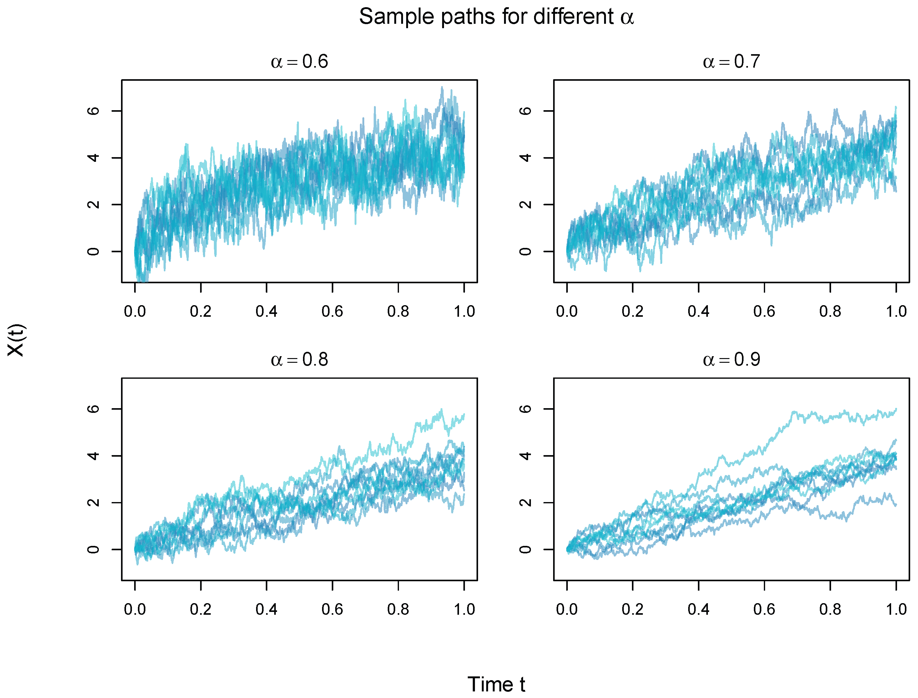
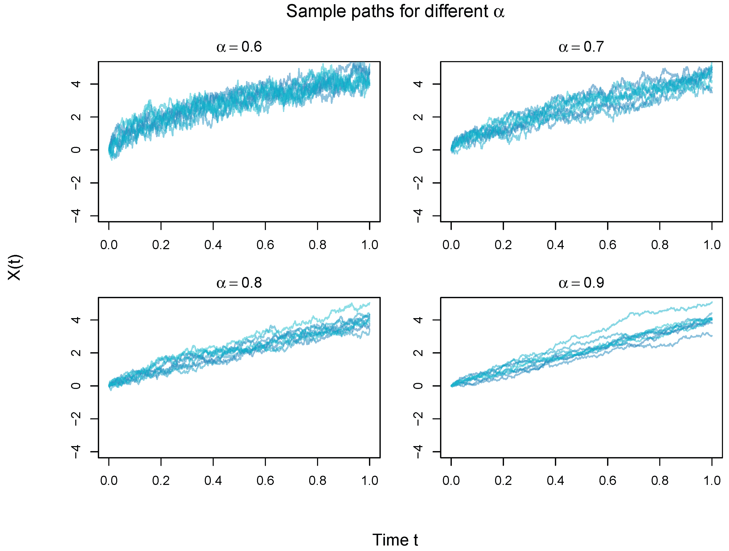
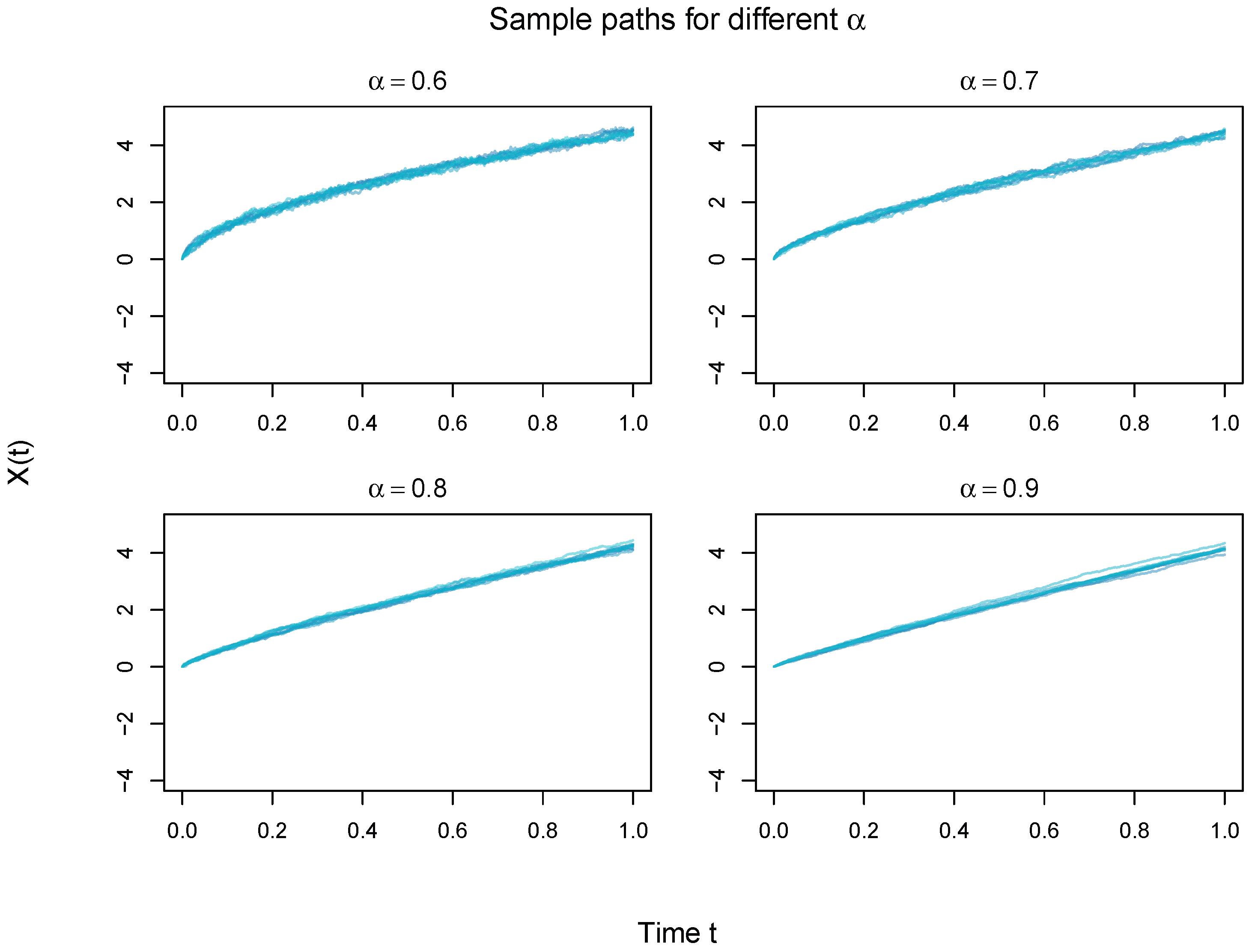
4.4. Simulation of Long-Memory Stochastic Trajectories

Simulated trajectories of a long-memory stochastic process are generated using the explicit integral form of the Caputo fractional equation, to illustrate the combined effects of temporal memory and volatility on process evolution. Simulations were performed for various values of the fractional order ${\displaystyle \alpha =0.6,0.7,0.8,0.9}$ and volatility ${\displaystyle \sigma =0.1,0.5,1}$. Each trajectory spans the interval ${\displaystyle [0,T]}$ with ${\displaystyle T=1}$, using ${\displaystyle n=800}$ discretization steps, which provide sufficient temporal resolution to accurately approximate the integral. The drift ${\displaystyle \mu =4}$ sets the mean trend of the process, while ${\displaystyle \sigma }$ controls the amplitude of stochastic fluctuations. The trajectories are obtained from

$$X\left(t_i\right)=X_0+{\displaystyle \frac{\mu t_i^{\alpha }}{\alpha \mathrm{\Gamma }\left(\alpha \right)}}+{\displaystyle \frac{\sigma }{\mathrm{\Gamma }\left(\alpha \right)}}\sum _{j=0}^{i-1}{(t_i-t_j)}^{\alpha -1}\mathrm{\Delta }{B}_j,i=1,\dots ,n.$$

where ${\displaystyle X_0=0}$, ${\displaystyle \mathrm{\Delta }t=T/n}$, ${\displaystyle \mathrm{\Delta }{B}_j\sim \mathcal{N}(0,\mathrm{\Delta }t)}$, and ${\displaystyle \mathrm{\Gamma }(·)}$ is the Gamma function. This formulation explicitly shows that each future value of the process depends on its entire past, weighted by the kernel ${\displaystyle {(t_i-t_j)}^{\alpha -1}}$, reflecting the long-memory effect.

• Effect of the fractional order ${\displaystyle \alpha }$

• Low ${\displaystyle \mathit{\alpha }}$ (0.6): The kernel gives less weight to recent past values, corresponding to short memory. Trajectories are more irregular, with rapid fluctuations even for low ${\displaystyle \sigma }$.
• Intermediate ${\displaystyle \mathit{\alpha }}$ (0.7–0.8): Memory is moderate. Trajectories are less noisy, but variability is still noticeable.
• High ${\displaystyle \mathit{\alpha }}$ (0.9): Long memory dominates. Trajectories are smoother and temporally correlated, with the effect of noise moderated by the process history.

• Impact of volatility ${\displaystyle \sigma }$

• ${\displaystyle \sigma =0.1}$: Trajectories are very smooth, and the memory effect is clearly visible.
• ${\displaystyle \sigma =0.5}$: Trajectories are moderately dispersed, with visible temporal correlation and memory effects.
• ${\displaystyle \sigma =1}$: Trajectories are highly irregular, but higher ${\displaystyle \alpha }$ values still introduce temporal correlation that partially tempers the noise.

This approach provides a clear visualization of how historical memory (${\displaystyle \alpha }$) and volatility (${\displaystyle \sigma }$) interact, offering an effective tool for comparing different fractional stochastic models, see Figure 1, Figure 2 and Figure 3.

5. Monte Carlo Assessment for the Caputo Fractional Stochastic System

This section reports a deliberately large-scale and methodologically stratified Monte Carlo investigation of the Caputo fractional stochastic system that serves as the computational engine for the simulation study. The objective extends beyond documenting numerical accuracy in a generic sense; rather, the experimental design is constructed to disentangle, as precisely as possible, three distinct layers of statistical complexity: the role of temporal resolution in approximating the continuous-time dynamics, the role of cross-trajectory replication in estimating the memory parameter, and the purely numerical effect of increasing the number of outer Monte Carlo replications used to stabilize empirical performance summaries. A further methodological consideration is to maintain a clear distinction between propositions that hold at the level of the continuous-time model and those that are valid only for the discretized model actually implemented in the simulation scheme. This distinction is especially important in fractional systems, where both the covariance structure and the effective information content of the sample are shaped by long-range dependence and by the specific discretization strategy employed.

5.1. Continuous-Time Model, Admissibility Conditions, and Matched Discrete Simulation

We consider the scalar Caputo-type fractional stochastic evolution on the compact time interval ${\displaystyle [0,T]}$, expressed through its mild representation:

$$X_t=X_0+{\displaystyle \frac{\mu }{\mathrm{\Gamma }\left(\alpha \right)}}{\int }_0^t{(t-s)}^{\alpha -1}ds+{\displaystyle \frac{\sigma }{\mathrm{\Gamma }\left(\alpha \right)}}{\int }_0^t{(t-s)}^{\alpha -1}dB\left(s\right),t\in [0,T],$$

(67)

where ${\displaystyle B}$ denotes a standard Brownian motion, ${\displaystyle \mu \in \mathbb{R}}$ is the drift coefficient, ${\displaystyle \sigma >0}$ is the diffusion coefficient, and ${\displaystyle \alpha \in (1/2,1)}$ is the fractional order. The lower bound ${\displaystyle \alpha >1/2}$ is not an implementation convention but the exact square-integrability threshold for the stochastic convolution. Specifically,

$${\int }_0^t{(t-s)}^{2\alpha -2}ds<\infty ⟺2\alpha -2>-1⟺\alpha >{\displaystyle \frac{1}{2}},$$

so the Gaussian stochastic integral is well defined in the ${\displaystyle L^2\left(\mathrm{\Omega }\right)}$ sense if and only if ${\displaystyle \alpha }$ exceeds one-half. The upper restriction ${\displaystyle \alpha <1}$ maintains the system in the genuinely fractional regime and excludes the classical first-order Markovian case. Throughout the numerical investigation, we fix the baseline configuration:

$$T=1,X_0=0,{\alpha }_0=0.8,{\mu }_0=0.1,{\sigma }_0=0.2,{\sigma }_0^2=0.04.$$

The choice ${\displaystyle {\alpha }_0=0.8}$ is deliberate: it remains sufficiently separated from the singular boundary ${\displaystyle \alpha =1/2}$ to avoid excessive instability arising from the kernel singularity, while still producing a clearly discernible memory effect in both the marginal variance law and the dependence geometry of the increments. The process is observed on the equidistant grid

$$t_i={\displaystyle \frac{iT}{n}},i=0,1,\dots ,n,$$

with mesh width ${\displaystyle \mathrm{\Delta }t=T/n}$. The deterministic component of (67) admits explicit integration:

$${\displaystyle \frac{\mu }{\mathrm{\Gamma }\left(\alpha \right)}}{\int }_0^t{(t-s)}^{\alpha -1}ds={\displaystyle \frac{\mu t^{\alpha }}{\mathrm{\Gamma }(\alpha +1)}}.$$

The trajectories employed in the Monte Carlo experiment are generated by a matched discrete simulation scheme. This terminology is intended to indicate that the simulation algorithm induces a discrete Gaussian model whose covariance structure is used exactly in the likelihood step. Specifically, if

$$\mathrm{\Delta }{B}_j:=B\left(t_{j+1}\right)-B\left(t_j\right)\sim \mathcal{N}(0,\mathrm{\Delta }t),j=0,\dots ,n-1,$$

denote independent Brownian increments, the implementation utilizes the left-point quadrature approximation

$$X_i^{\left(n\right)}:=X_{t_i}^{\left(n\right)}=X_0+{\displaystyle \frac{\mu t_i^{\alpha }}{\mathrm{\Gamma }(\alpha +1)}}+{\displaystyle \frac{\sigma }{\mathrm{\Gamma }\left(\alpha \right)}}\sum _{j=0}^{i-1}{(t_i-t_j)}^{\alpha -1}\mathrm{\Delta }{B}_j,i=1,\dots ,n.$$

(68)

It is important to note that (68) constitutes a discretization of the continuous-time mild representation, not an exact simulation of the finite-dimensional law of the continuous process (67). Consequently, all model-based likelihood calculations reported subsequently are matched to the discrete Gaussian model actually generated by (68). This eliminates any hidden mismatch between the simulation engine and the inferential procedure. For each configuration ${\displaystyle (\alpha ,n,T)}$, the lower-triangular fractional kernel weights

$$g_{i,j}^{(\alpha ,n)}:={(t_i-t_j)}^{\alpha -1},0\le j<i\le n,$$

are precomputed once and reused across all replications under the same configuration. This approach is both computationally advantageous and statistically coherent: it preserves the deterministic fractional geometry exactly across replications and shifts the numerical burden toward the stochastic component of the experiment.

5.2. Hierarchical Simulation Design and Inferential Objectives

The Monte Carlo study is organized into three design regimes reflecting increasing levels of comprehensiveness:

$${\mathcal{N}}_{\mathrm{expl}}=\{100,250,500\},{\mathcal{N}}_{\mathrm{conf}}=\{250,500,1000\},{\mathcal{N}}_{\mathrm{comp}}=\{100,250,500,1000,2000\}.$$

In the comprehensive regime, we additionally vary two auxiliary dimensions:

• ${\displaystyle N_{\mathrm{MC}}}$, the number of outer Monte Carlo replications;
• ${\displaystyle N_{\mathrm{var}}}$, the number of independent trajectories employed by the variance-growth estimator of the memory parameter.

The distinction between these two quantities is fundamental and must be maintained with clear conceptual separation throughout. The quantity ${\displaystyle N_{\mathrm{MC}}}$ is a numerical stabilization parameter: it controls only the precision with which empirical means, biases, root mean squared errors, and coverage probabilities are approximated. It is, therefore, not part of the statistical information set of any estimator. By contrast, ${\displaystyle N_{\mathrm{var}}}$ directly affects the information available to the variance-growth estimator of ${\displaystyle \alpha }$, because that estimator reconstructs the marginal variance curve from an ensemble of independent trajectories.

This distinction carries immediate methodological consequences. Among the four estimators examined below, only ${\displaystyle {\widehat{\alpha }}_{\mathrm{var}}}$ employs ${\displaystyle N_{\mathrm{var}}}$ as a genuine data dimension. The wavelet-type estimator ${\displaystyle {\widehat{\alpha }}_{\mathrm{wave}}}$, as well as the Gaussian likelihood estimators ${\displaystyle \widehat{\mu }}$ and ${\displaystyle {\widehat{\sigma }}^2}$, are computed from a single trajectory and, therefore, do not depend structurally on ${\displaystyle N_{\mathrm{var}}}$. Whenever their numerical summaries are displayed across rows indexed by different values of ${\displaystyle N_{\mathrm{var}}}$, the resulting fluctuations should be interpreted solely as ordinary Monte Carlo variation induced by rerunning the global experiment under different configurations; they should not be read as substantive statistical effects.

The comprehensive design, thus, addresses three distinct questions:

• How does increased temporal resolution ${\displaystyle n}$ improve recovery of the memory parameter and of the finite-dimensional coefficients?
• How stable are the empirical performance summaries as the outer Monte Carlo size ${\displaystyle N_{\mathrm{MC}}}$ increases?
• To what extent does independent path replication enhance the ensemble-based estimator of ${\displaystyle \alpha }$ relative to a single-path multiscale estimator?

This three-way decomposition is statistically more informative than a one-factor grid over sample size alone, since it prevents the study from conflating estimator identifiability, discretization refinement, and Monte Carlo approximation accuracy.

5.3. Estimation Procedures

5.3.1. Variance-Growth Estimator of the Memory Parameter

At the level of the continuous-time model (67), the marginal variance satisfies

$$Var\left\{X_t\right\}={\displaystyle \frac{{\sigma }^2}{\mathrm{\Gamma }{\left(\alpha \right)}^2}}{\int }_0^t{(t-s)}^{2\alpha -2}ds={\displaystyle \frac{{\sigma }^2}{(2\alpha -1)\mathrm{\Gamma }{\left(\alpha \right)}^2}}{t}^{2\alpha -1}.$$

Consequently,

$$logVar\left\{X_t\right\}=C+(2\alpha -1)logt,$$

where ${\displaystyle C}$ is a constant depending on ${\displaystyle {\sigma }^2}$ and ${\displaystyle \alpha }$ but not on ${\displaystyle t}$. This exact power-law identity motivates the first estimator of ${\displaystyle \alpha }$.

For each observation time ${\displaystyle t_i}$, the empirical variance across ${\displaystyle N_{\mathrm{var}}}$ independent trajectories is computed as

$${\widehat{v}}_i={\displaystyle \frac{1}{N_{\mathrm{var}}-1}}\sum _{\ell =1}^{N_{\mathrm{var}}}{\left(X_{i,\ell }^{\left(n\right)}-{\overline{X}}_i^{\left(n\right)}\right)}^2,{\overline{X}}_i^{\left(n\right)}={\displaystyle \frac{1}{N_{\mathrm{var}}}}\sum _{\ell =1}^{N_{\mathrm{var}}}{X}_{i,\ell }^{\left(n\right)},$$

where ${\displaystyle X_{i,\ell }^{\left(n\right)}}$ denotes the ${\displaystyle \ell }$th simulated trajectory at time ${\displaystyle t_i}$. A log-linear regression

$$log{\widehat{v}}_i=c+\beta log{t}_i+{\epsilon }_i$$

is then fitted over the grid points, and the estimator is defined by

$${\widehat{\alpha }}_{\mathrm{var}}={\displaystyle \frac{\widehat{\beta }+1}{2}}.$$

This estimator is theoretically well aligned with the underlying continuous-time model because it exploits an exact second-order scaling relation rather than a heuristic roughness proxy. In the simulation study, it is applied to data generated from the matched discrete approximation (68), so its finite-sample performance reflects both the quality of the variance reconstruction and the effect of time discretization.

5.3.2. Wavelet-Type Multiscale Estimator of the Memory Parameter

The second estimator of ${\displaystyle \alpha }$ is constructed from a single trajectory and is based on a transparent Haar-type multiscale contrast scheme. Let

$${\tilde{X}}_i^{\left(n\right)}=X_i^{\left(n\right)}-{\displaystyle \frac{1}{n}}\sum _{m=1}^n{X}_m^{\left(n\right)}$$

denote the globally centered trajectory. For each dyadic level ${\displaystyle j\ge 1}$, define the block length

$$m_j=2^j,M_j=⌊{\displaystyle \frac{n}{m_j}}⌋,$$

and the associated block averages

$${\overline{X}}_{j,r}={\displaystyle \frac{1}{m_j}}\sum _{u=(r-1)m_j+1}^{r{m}_j}{\tilde{X}}_u^{\left(n\right)},r=1,\dots ,M_j.$$

Next, define adjacent-block contrasts

$$D_{j,k}={\overline{X}}_{j,2k}-{\overline{X}}_{j,2k-1},k=1,\dots ,K_j,K_j=⌊{\displaystyle \frac{M_j}{2}}⌋,$$

and the empirical contrast variance

$$S_j^2={\displaystyle \frac{1}{K_j}}\sum _{k=1}^{K_j}{D}_{j,k}^2.$$

The estimator is obtained from a regression of ${\displaystyle log{S}_j^2}$ on ${\displaystyle log{m}_j=jlog2}$. If ${\displaystyle \widehat{s}}$ denotes the fitted slope, the implemented calibration is

$${\widehat{\alpha }}_{\mathrm{wave}}={\displaystyle \frac{\widehat{s}+1}{2}}.$$

We deliberately characterize this procedure as wavelet-type rather than as a fully exact orthogonal-wavelet estimator. The use of explicit adjacent Haar-style block contrasts offers complete transparency and renders the scale statistic easily interpretable. However, two important qualifications merit attention. First, because the process is nonstationary and the procedure is applied to a globally centered trajectory in levels rather than to a stationary increment sequence, the estimator should be understood as a multiscale empirical proxy for the memory parameter rather than as an exact semiparametric estimator justified by a fully developed asymptotic theory for the present model. Second, global centering does not entirely remove the effect of the deterministic drift component ${\displaystyle \mu t^{\alpha }/\mathrm{\Gamma }(\alpha +1)}$ on the contrast variances; with the baseline choice ${\displaystyle {\mu }_0=0.1}$, this effect is expected to be limited, although it is not isolated separately in the Monte Carlo study. The admissible scale range is truncated according to

$$J\le min\{5,\lfloor {log}_2\left(n\right)\rfloor -2\},$$

so as to exclude the coarsest dyadic levels, where the number of available contrasts becomes too small for stable variance estimation and reliable regression.

5.3.3. Gaussian Likelihood Estimation of ${\displaystyle (\mu ,{\sigma }^2)}$ Conditional on ${\displaystyle \alpha }$

For the parametric step, we work with the increment vector

$$Y_i=X_i^{\left(n\right)}-X_{i-1}^{\left(n\right)},i=1,\dots ,n.$$

Under the matched discrete simulation scheme (68), the vector ${\displaystyle Y={(Y_1,\dots ,Y_n)}^{\top }}$ is Gaussian. Its mean is

$$\mathbb{E}\left(Y_i\right)=\mu b_{\alpha ,i},b_{\alpha ,i}={\displaystyle \frac{t_i^{\alpha }-t_{i-1}^{\alpha }}{\mathrm{\Gamma }(\alpha +1)}},i=1,\dots ,n.$$

Its covariance is induced by the same discrete fractional kernel used in the simulator. Writing ${\displaystyle g_{i,j}^{(\alpha ,n)}={(t_i-t_j)}^{\alpha -1}}$ with the convention ${\displaystyle g_{0,j}^{(\alpha ,n)}:=0}$, one obtains

$$Y_i=\mu b_{\alpha ,i}+{\displaystyle \frac{\sigma }{\mathrm{\Gamma }\left(\alpha \right)}}\sum _{j=0}^{n-1}\left(g_{i,j}^{(\alpha ,n)}-g_{i-1,j}^{(\alpha ,n)}\right)\mathrm{\Delta }{B}_j.$$

Hence

$$Y\sim {\mathcal{N}}_n\left(\mu b_{\alpha },{\sigma }^2{C}_{\alpha }\right),$$

where ${\displaystyle b_{\alpha }={(b_{\alpha ,1},\dots ,b_{\alpha ,n})}^{\top }}$ and

$${\left(C_{\alpha }\right)}_{ik}={\displaystyle \frac{1}{\mathrm{\Gamma }{\left(\alpha \right)}^2}}\sum _{j=0}^{n-1}\left(g_{i,j}^{(\alpha ,n)}-g_{i-1,j}^{(\alpha ,n)}\right)\left(g_{k,j}^{(\alpha ,n)}-g_{k-1,j}^{(\alpha ,n)}\right)·Var\left(\mathrm{\Delta }{B}_j\right),1\le i,k\le n.$$

(69)

Since ${\displaystyle Var\left(\mathrm{\Delta }{B}_j\right)=\mathrm{\Delta }t}$, the covariance matrix can be written explicitly as

$${\left(C_{\alpha }\right)}_{ik}={\displaystyle \frac{\mathrm{\Delta }t}{\mathrm{\Gamma }{\left(\alpha \right)}^2}}\sum _{j=0}^{n-1}\left(g_{i,j}^{(\alpha ,n)}-g_{i-1,j}^{(\alpha ,n)}\right)\left(g_{k,j}^{(\alpha ,n)}-g_{k-1,j}^{(\alpha ,n)}\right).$$

(70)

This point deserves emphasis: the covariance matrix employed in inference is exact for the discrete Gaussian model actually simulated. The factor ${\displaystyle \mathrm{\Delta }t}$ arises directly from the variance of the Brownian increments and ensures dimensional consistency; the kernel weights ${\displaystyle g_{i,j}^{(\alpha ,n)}}$ carry units of ${\displaystyle {\left(\mathrm{time}\right)}^{\alpha -1}}$, so the overall expression has the correct scaling for a covariance matrix. The likelihood step is, therefore, internally matched to the Monte Carlo generator and does not impose an artificial independence assumption or an external approximation unrelated to the implemented scheme. Conditional on a fixed value of ${\displaystyle \alpha }$, the generalized least-squares maximum likelihood estimator of ${\displaystyle \mu }$ is

$$\widehat{\mu }={\displaystyle \frac{b_{\alpha }^{\top }{C}_{\alpha }^{-1}Y}{b_{\alpha }^{\top }{C}_{\alpha }^{-1}{b}_{\alpha }}},$$

and the corresponding estimator of ${\displaystyle {\sigma }^2}$ is

$${\widehat{\sigma }}^2={\displaystyle \frac{1}{n}}{\left(Y-\widehat{\mu }{b}_{\alpha }\right)}^{\top }{C}_{\alpha }^{-1}\left(Y-\widehat{\mu }{b}_{\alpha }\right).$$

The study reports nominal ${\displaystyle 95\%}$ confidence intervals constructed from the Gaussian likelihood output. For ${\displaystyle \mu }$, the interval is based on the usual Wald approximation using the estimated standard error associated with the generalized least-squares fit. For ${\displaystyle {\sigma }^2}$, the reported interval is likewise derived from the corresponding Gaussian likelihood scale estimate. All likelihood results are obtained conditionally on the true value of ${\displaystyle \alpha }$. The parametric step should, therefore, be interpreted as an oracle second-stage experiment. This is not a weakness of the design; on the contrary, it is the cleanest way to isolate the intrinsic finite-sample behavior of the Gaussian likelihood step from the additional variability that would arise if an estimated memory parameter were plugged into the covariance matrix. In fractional models, such a decomposition is often essential because the dependence of ${\displaystyle C_{\alpha }}$ on ${\displaystyle \alpha }$ is highly nonlinear, and the propagation of estimation uncertainty through this nonlinear mapping warrants a separate investigation.

5.4. Performance Criteria and Reporting Strategy

For each design point and for each estimator ${\displaystyle \widehat{\theta }}$, let ${\displaystyle {\widehat{\theta }}^{\left(1\right)},\dots ,{\widehat{\theta }}^{\left(N_{\mathrm{MC}}\right)}}$ denote the Monte Carlo replicates. We report the empirical mean

$${\overline{\theta }}_{\mathrm{MC}}={\displaystyle \frac{1}{N_{\mathrm{MC}}}}\sum _{r=1}^{N_{\mathrm{MC}}}{\widehat{\theta }}^{\left(r\right)},$$

the empirical standard deviation

$${sd}_{\mathrm{MC}}\left(\widehat{\theta }\right)={\left\{{\displaystyle \frac{1}{N_{\mathrm{MC}}-1}}\sum _{r=1}^{N_{\mathrm{MC}}}{\left({\widehat{\theta }}^{\left(r\right)}-{\overline{\theta }}_{\mathrm{MC}}\right)}^2\right\}}^{1/2},$$

the empirical bias

$${Bias}_{\mathrm{MC}}\left(\widehat{\theta }\right)={\overline{\theta }}_{\mathrm{MC}}-\theta ,$$

and the empirical root mean squared error

$${RMSE}_{\mathrm{MC}}\left(\widehat{\theta }\right)={\left\{{\displaystyle \frac{1}{N_{\mathrm{MC}}}}\sum _{r=1}^{N_{\mathrm{MC}}}{\left({\widehat{\theta }}^{\left(r\right)}-\theta \right)}^2\right\}}^{1/2}.$$

For the likelihood-based estimators ${\displaystyle \widehat{\mu }}$ and ${\displaystyle {\widehat{\sigma }}^2}$, we also report the empirical coverage probabilities of nominal ${\displaystyle 95\%}$ confidence intervals:

$${Coverage}_{\mathrm{MC}}\left(\widehat{\theta }\right)={\displaystyle \frac{1}{N_{\mathrm{MC}}}}\sum _{r=1}^{N_{\mathrm{MC}}}\mathbf{1}\{\theta \in {\mathrm{CI}}_{0.95}^{\left(r\right)}\}.$$

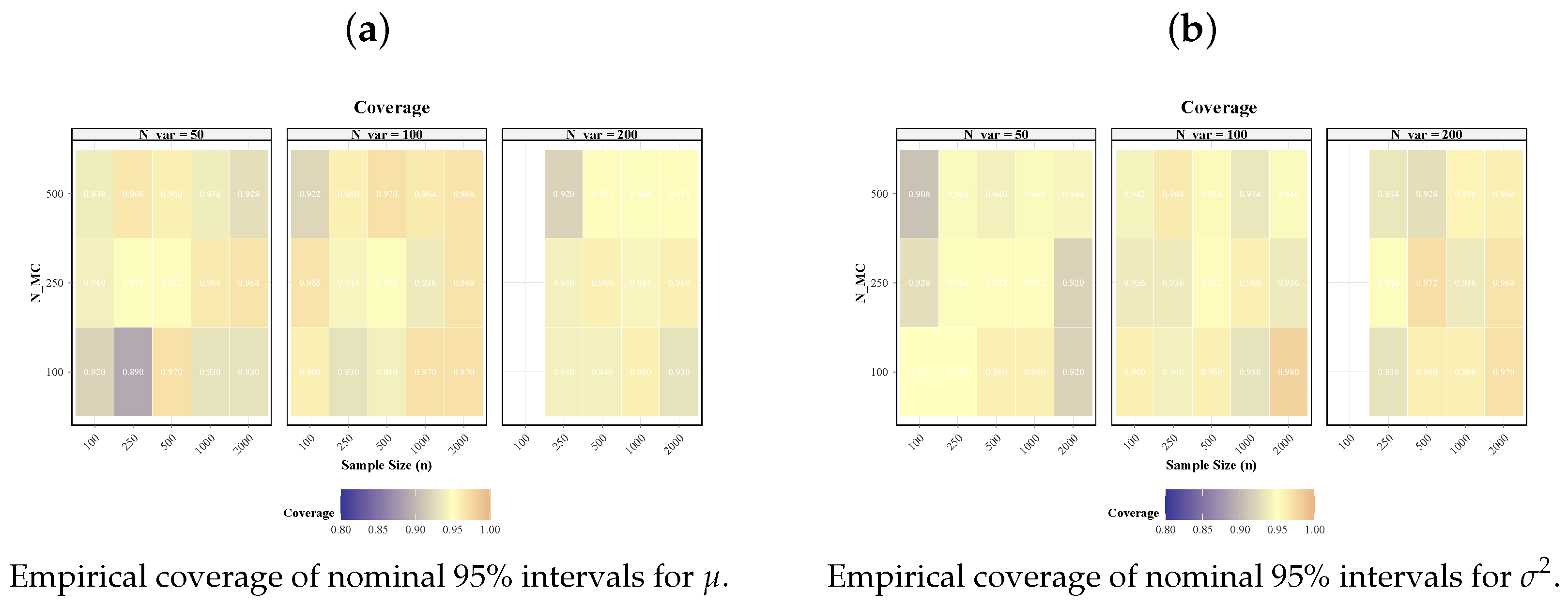
The numerical evidence is summarized in

Table 1. Monte Carlo performance of the two estimators of the fractional order ${\displaystyle \alpha }$ under the comprehensive simulation design. The true value is ${\displaystyle {\alpha }_0=0.8}$.

${\displaystyle \mathit{n}}$	${\displaystyle {\mathit{N}}_{\mathbf{MC}}}$	${\displaystyle {\mathit{N}}_{\mathbf{var}}}$	${\displaystyle {\widehat{\mathit{\alpha }}}_{\mathbf{var}}}$	RMSE ${\displaystyle \left({\widehat{\mathit{\alpha }}}_{\mathbf{var}}\right)}$	${\displaystyle {\widehat{\mathit{\alpha }}}_{\mathbf{wave}}}$	RMSE ${\displaystyle \left({\widehat{\mathit{\alpha }}}_{\mathbf{wave}}\right)}$
100	100	50	0.8355	0.0504	0.7573	0.1645
100	100	100	0.8373	0.0446	0.7407	0.1667
100	250	50	0.8355	0.0537	0.7536	0.1627
100	250	100	0.8307	0.0425	0.7642	0.1478
100	500	50	0.8333	0.0526	0.7617	0.1593
100	500	100	0.8337	0.0424	0.7619	0.1561
250	100	50	0.8270	0.0447	0.8033	0.1054
250	100	100	0.8214	0.0313	0.7823	0.1242
250	100	200	0.8249	0.0305	0.7924	0.1102
250	250	50	0.8239	0.0425	0.7893	0.1252
250	250	100	0.8246	0.0366	0.7786	0.1131
250	250	200	0.8219	0.0281	0.7870	0.1150
250	500	50	0.8255	0.0452	0.7846	0.1154
250	500	100	0.8235	0.0338	0.7869	0.1135
250	500	200	0.8229	0.0280	0.7775	0.1149
500	100	50	0.8127	0.0405	0.8047	0.0713
500	100	100	0.8139	0.0254	0.8083	0.0678
500	100	200	0.8193	0.0259	0.8053	0.0722
500	250	50	0.8227	0.0425	0.8029	0.0797
500	250	100	0.8162	0.0284	0.7972	0.0776
500	250	200	0.8167	0.0237	0.7987	0.0746
500	500	50	0.8177	0.0397	0.8029	0.0746
500	500	100	0.8163	0.0290	0.8059	0.0718
500	500	200	0.8173	0.0241	0.8075	0.0697
1000	100	50	0.8088	0.0340	0.8128	0.0477
1000	100	100	0.8148	0.0283	0.8166	0.0494
1000	100	200	0.8109	0.0201	0.8050	0.0460
1000	250	50	0.8096	0.0329	0.8063	0.0456
1000	250	100	0.8105	0.0262	0.8154	0.0480
1000	250	200	0.8136	0.0206	0.8079	0.0496
1000	500	50	0.8144	0.0352	0.8138	0.0503
1000	500	100	0.8115	0.0259	0.8057	0.0488
1000	500	200	0.8134	0.0216	0.8082	0.0483
2000	100	50	0.8115	0.0370	0.8142	0.0350
2000	100	100	0.8104	0.0246	0.8099	0.0357
2000	100	200	0.8079	0.0195	0.8118	0.0356
2000	250	50	0.8069	0.0344	0.8110	0.0354
2000	250	100	0.8080	0.0250	0.8123	0.0339
2000	250	200	0.8080	0.0186	0.8121	0.0378
2000	500	50	0.8072	0.0338	0.8100	0.0347
2000	500	100	0.8096	0.0263	0.8113	0.0358
2000	500	200	0.8092	0.0186	0.8113	0.0349

,

Table 2. Monte Carlo performance of the oracle Gaussian likelihood estimator of the drift coefficient ${\displaystyle \mu }$ under the comprehensive simulation design. The true value is ${\displaystyle {\mu }_0=0.1}$. Rows indexed by different values of ${\displaystyle N_{\mathrm{var}}}$ are retained for alignment with the global design, although ${\displaystyle N_{\mathrm{var}}}$ is not part of the information set of ${\displaystyle \widehat{\mu }}$.

${\displaystyle \mathit{n}}$	${\displaystyle {\mathit{N}}_{\mathbf{MC}}}$	${\displaystyle {\mathit{N}}_{\mathbf{var}}}$	${\displaystyle \widehat{\mathit{\mu }}}$	RMSE ${\displaystyle \left(\widehat{\mathit{\mu }}\right)}$	Coverage ${\displaystyle \left(\mathit{\mu }\right)}$
100	100	50	0.0943	0.2140	0.920
100	100	100	0.0907	0.1849	0.960
100	250	50	0.0870	0.2063	0.940
100	250	100	0.1278	0.1812	0.968
100	500	50	0.0912	0.1969	0.938
100	500	100	0.0971	0.2081	0.922
250	100	50	0.1066	0.2222	0.890
250	100	100	0.0796	0.2020	0.930
250	100	200	0.1201	0.2025	0.940
250	250	50	0.0980	0.1912	0.948
250	250	100	0.1292	0.2067	0.944
250	250	200	0.1051	0.2151	0.940
250	500	50	0.1029	0.1882	0.966
250	500	100	0.1077	0.1906	0.960
250	500	200	0.1113	0.2039	0.920
500	100	50	0.1248	0.1896	0.970
500	100	100	0.0576	0.2236	0.940
500	100	200	0.0765	0.1949	0.940
500	250	50	0.0943	0.1970	0.952
500	250	100	0.1239	0.2057	0.948
500	250	200	0.1196	0.1952	0.960
500	500	50	0.1145	0.1865	0.960
500	500	100	0.0953	0.1888	0.970
500	500	200	0.0923	0.1985	0.952
1000	100	50	0.0874	0.2164	0.930
1000	100	100	0.1009	0.2066	0.970
1000	100	200	0.0752	0.1991	0.960
1000	250	50	0.0912	0.1963	0.964
1000	250	100	0.0780	0.2055	0.936
1000	250	200	0.1014	0.1968	0.944
1000	500	50	0.0970	0.2034	0.938
1000	500	100	0.0931	0.1867	0.964
1000	500	200	0.0911	0.1973	0.948
2000	100	50	0.1374	0.1983	0.930
2000	100	100	0.1423	0.1778	0.970
2000	100	200	0.0947	0.2097	0.930
2000	250	50	0.1021	0.2013	0.968
2000	250	100	0.1013	0.1950	0.968
2000	250	200	0.0920	0.2055	0.960
2000	500	50	0.1131	0.2084	0.928
2000	500	100	0.1019	0.1887	0.968
2000	500	200	0.0869	0.2001	0.952

and

Table 3. Monte Carlo performance of the oracle Gaussian likelihood estimator of the diffusion coefficient ${\displaystyle {\sigma }^2}$ under the comprehensive simulation design. The true value is ${\displaystyle {\sigma }_0^2=0.04}$. Rows indexed by different values of ${\displaystyle N_{\mathrm{var}}}$ are retained for alignment with the global design, although ${\displaystyle N_{\mathrm{var}}}$ is not part of the information set of ${\displaystyle {\widehat{\sigma }}^2}$.

${\displaystyle \mathit{n}}$	${\displaystyle {\mathit{N}}_{\mathbf{MC}}}$	${\displaystyle {\mathit{N}}_{\mathbf{var}}}$	${\displaystyle {\widehat{\mathit{\sigma }}}^2}$	RMSE ${\displaystyle \left({\widehat{\mathit{\sigma }}}^2\right)}$	Coverage ${\displaystyle \left({\mathit{\sigma }}^2\right)}$
100	100	50	0.039407	0.005651	0.950
100	100	100	0.039987	0.005718	0.960
100	250	50	0.039807	0.005725	0.928
100	250	100	0.039448	0.005123	0.936
100	500	50	0.039497	0.006266	0.908
100	500	100	0.039493	0.005311	0.942
250	100	50	0.040026	0.003654	0.950
250	100	100	0.039248	0.003490	0.940
250	100	200	0.040045	0.003826	0.930
250	250	50	0.040114	0.003542	0.948
250	250	100	0.039976	0.003659	0.936
250	250	200	0.040021	0.003500	0.948
250	500	50	0.039742	0.003557	0.946
250	500	100	0.039893	0.003423	0.964
250	500	200	0.039818	0.003550	0.934
500	100	50	0.039756	0.002190	0.960
500	100	100	0.039606	0.002284	0.960
500	100	200	0.040213	0.002706	0.960
500	250	50	0.039832	0.002431	0.952
500	250	100	0.039874	0.002369	0.952
500	250	200	0.039718	0.002295	0.972
500	500	50	0.040115	0.002538	0.940
500	500	100	0.039976	0.002502	0.954
500	500	200	0.040025	0.002723	0.928
1000	100	50	0.040052	0.001821	0.960
1000	100	100	0.039725	0.001910	0.930
1000	100	200	0.039949	0.001825	0.960
1000	250	50	0.040086	0.001800	0.952
1000	250	100	0.039796	0.001652	0.960
1000	250	200	0.039920	0.001771	0.936
1000	500	50	0.039969	0.001761	0.946
1000	500	100	0.040013	0.001822	0.934
1000	500	200	0.039911	0.001796	0.958
2000	100	50	0.040068	0.001275	0.920
2000	100	100	0.040118	0.001195	0.980
2000	100	200	0.040077	0.001241	0.970
2000	250	50	0.039819	0.001313	0.920
2000	250	100	0.039985	0.001367	0.936
2000	250	200	0.039987	0.001208	0.968
2000	500	50	0.040053	0.001278	0.944
2000	500	100	0.040001	0.001282	0.946
2000	500	200	0.039988	0.001273	0.960

and in Figure 4, Figure 5, Figure 6 and Figure 7. The tables provide exact numerical summaries, whereas the figures expose structural features that are difficult to discern from tables alone, including monotonicity in ${\displaystyle n}$, sensitivity to ${\displaystyle N_{\mathrm{var}}}$, stabilization with respect to ${\displaystyle N_{\mathrm{MC}}}$, and the geometry of increment dependence.

5.5. Monte Carlo Results for the Memory Parameter ${\displaystyle \alpha }$

Table 1 reports the finite-sample behavior of the two estimators of the memory parameter. The most salient conclusion is that the two procedures operate in genuinely different statistical regimes and should, therefore, be evaluated according to distinct information channels.

The variance-growth estimator ${\displaystyle {\widehat{\alpha }}_{\mathrm{var}}}$ displays a small but visible positive bias in the lowest-resolution settings. For example, when ${\displaystyle n=100}$, its empirical mean typically ranges from ${\displaystyle 0.83}$ to ${\displaystyle 0.84}$, although the true value is ${\displaystyle {\alpha }_0=0.8}$. This behavior is not surprising. The estimator is based on a regression of empirical log-variances, and finite-sample irregularities in the variance curve are amplified by the logarithmic transformation, particularly at the lower end of the time horizon. However, the same table also shows that the RMSE decreases substantially as ${\displaystyle N_{\mathrm{var}}}$ increases. This is entirely coherent with the construction of the estimator: additional independent trajectories improve the reconstruction of the marginal second-order structure and are, therefore, converted directly into increased precision.

The wavelet-type estimator ${\displaystyle {\widehat{\alpha }}_{\mathrm{wave}}}$ behaves differently. At coarse temporal resolutions, it tends to underestimate ${\displaystyle \alpha }$, particularly when ${\displaystyle n=100}$, but it improves substantially as ${\displaystyle n}$ grows. This is exactly what one would expect from a single-trajectory multiscale method. Its principal source of information is temporal resolution, not replication. By the time ${\displaystyle n=2000}$, its RMSE is of order ${\displaystyle 3.5\times {10}^{-2}}$, whereas the variance-growth estimator can achieve RMSE below ${\displaystyle 2\times {10}^{-2}}$ when both ${\displaystyle n}$ and ${\displaystyle N_{\mathrm{var}}}$ are sufficiently large.

The correct interpretation of the table is, therefore, one of complementarity rather than uniform dominance. The variance-growth procedure is replication-driven; the wavelet-type procedure is resolution-driven. Since ${\displaystyle N_{\mathrm{var}}}$ does not belong to the information set of ${\displaystyle {\widehat{\alpha }}_{\mathrm{wave}}}$, the modest fluctuations of the latter across rows indexed by different values of ${\displaystyle N_{\mathrm{var}}}$ should be interpreted as ordinary Monte Carlo variation and not as a structural statistical effect.

5.6. Monte Carlo Results for the Drift Parameter ${\displaystyle \mu }$

Table 2 reports the oracle Gaussian likelihood results for the drift parameter. The most striking feature is not a rapid collapse of RMSE with increasing ${\displaystyle n}$, but rather the persistence of moderate variability throughout the design grid. This deserves careful interpretation. In the present model, the drift enters through the deterministic fractional profile ${\displaystyle t\mapsto t^{\alpha }/\mathrm{\Gamma }(\alpha +1)}$, but inference is conducted on increments whose covariance structure exhibits strong dependence and whose stochastic component propagates nonlocally through the fractional kernel. Relative to this dependence-driven noise, the drift signal is comparatively weak. One should not, therefore, expect the same finite-sample sharpness for ${\displaystyle \mu }$ as for the diffusion coefficient.

The table shows that the estimator remains broadly centered around the true value ${\displaystyle {\mu }_0=0.1}$, with no evidence of severe systematic distortion. The RMSE values remain in a relatively narrow range, roughly between ${\displaystyle 0.18}$ and ${\displaystyle 0.22}$, indicating that point estimation of the drift is intrinsically delicate in this fractional setting. From an inferential perspective, however, the results are more reassuring. The empirical coverage of the nominal ${\displaystyle 95\%}$ intervals is generally close to the target level, with most values falling between ${\displaystyle 0.93}$ and ${\displaystyle 0.97}$, although a few low-resolution configurations exhibit more noticeable undercoverage or slight overcoverage. The dominant message of the table is, therefore, not one of spectacular point-estimation efficiency, but rather one of acceptable finite-sample calibration for interval inference under the correctly specified discrete covariance structure.

Since the likelihood analysis is performed conditionally on the true value of ${\displaystyle \alpha }$, the conclusion must be interpreted with appropriate precision: the matched Gaussian likelihood appears inferentially reliable for the drift parameter in the oracle-${\displaystyle \alpha }$ regime, with coverage properties that are broadly satisfactory though not uniformly exact.

5.7. Monte Carlo Results for the Diffusion Parameter ${\displaystyle {\sigma }^2}$

The finite-sample behavior of the diffusion estimator, reported in Table 3, is considerably sharper. This is arguably the most stable component of the entire simulation study. The estimated means remain extremely close to the true value ${\displaystyle {\sigma }_0^2=0.04}$ throughout the design grid, with deviations that are numerically very small relative to the scale of the parameter itself. More importantly, the RMSE decreases systematically as the temporal resolution increases: values of order ${\displaystyle 5\times {10}^{-3}}$ at ${\displaystyle n=100}$ fall to approximately ${\displaystyle 1.2\times {10}^{-3}}$ at ${\displaystyle n=2000}$.

This behavior is entirely consistent with the statistical role played by ${\displaystyle {\sigma }^2}$ in the model. The diffusion coefficient controls the global amplitude of the covariance structure, and once the correct fractional dependence is encoded into the Gaussian likelihood, that global scale can be recovered much more stably than the drift coefficient. The table, therefore, suggests that, under the oracle specification of ${\displaystyle \alpha }$, the principal finite-sample challenge does not lie in identifying the overall variance scale.

The coverage results reinforce the same conclusion. The empirical coverage of the nominal ${\displaystyle 95\%}$ intervals is in most cases close to the target level, typically ranging between ${\displaystyle 0.92}$ and ${\displaystyle 0.97}$, though some low-resolution configurations exhibit mild undercoverage and a few others show slight overcoverage. Overall, both point estimation and interval estimation for ${\displaystyle {\sigma }^2}$ appear satisfactory under the matched discrete Gaussian model. In methodological terms, this indicates that the main statistical burden in the Caputo system lies in recovering the memory exponent and, to a lesser extent, the drift component, rather than the diffusion scale.

5.8. Graphical Synthesis and Detailed Interpretation

The graphical component complements the numerical tables along four principal directions: risk visualization, interval calibration, empirical convergence, and dependence geometry.

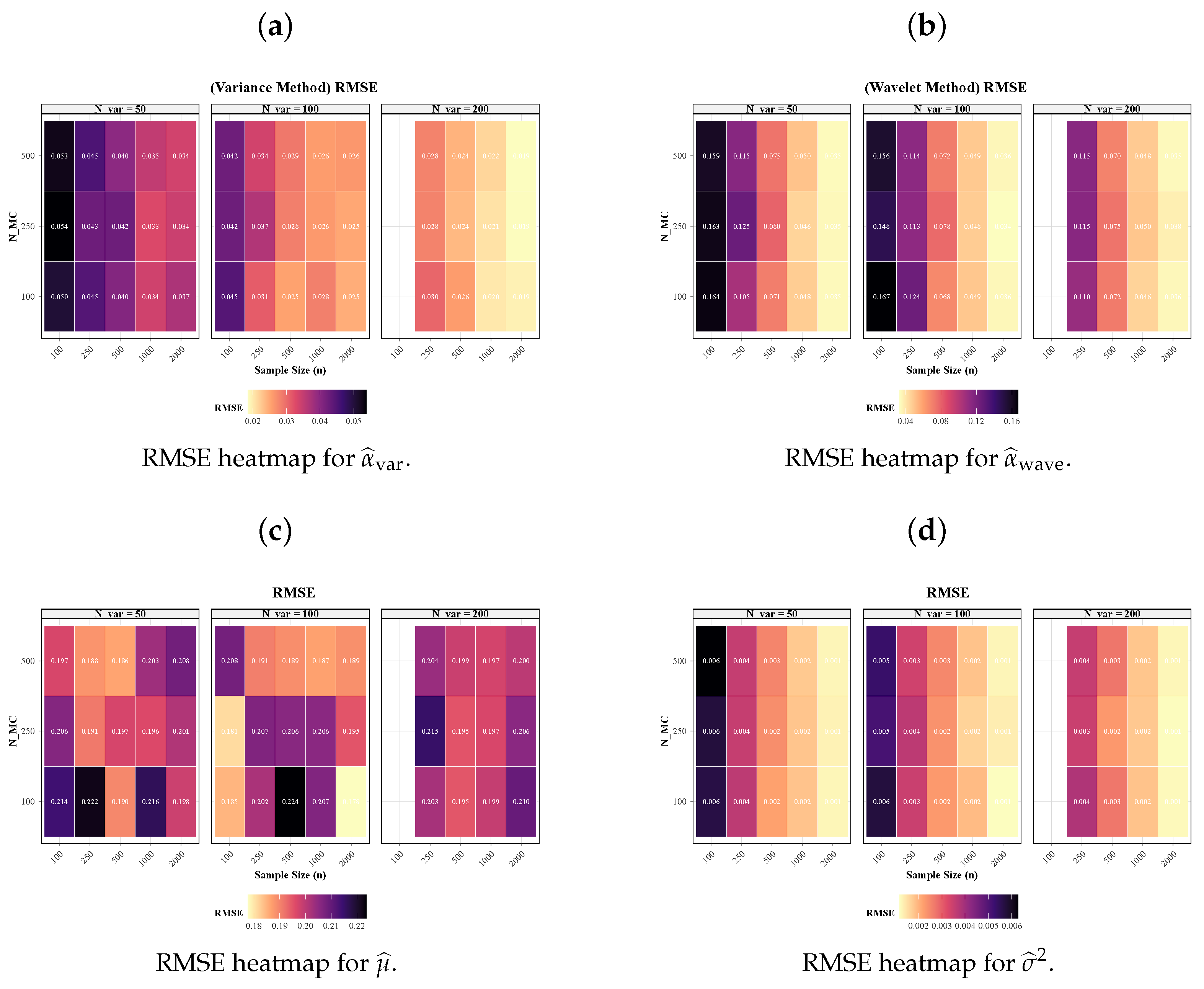
Figure 4 displays RMSE heatmaps for the four estimators. These panels render the different statistical regimes particularly transparent. In panel (a), corresponding to ${\displaystyle {\widehat{\alpha }}_{\mathrm{var}}}$, the surface improves materially as ${\displaystyle N_{\mathrm{var}}}$ increases, confirming that this estimator is genuinely driven by cross-sectional path replication. By contrast, panel (b), corresponding to ${\displaystyle {\widehat{\alpha }}_{\mathrm{wave}}}$, is governed primarily by the temporal resolution ${\displaystyle n}$, reflecting the single-path multiscale nature of the procedure. Panels (c) and (d) exhibit the same contrast on the parametric side: diffusion estimation stabilizes more cleanly than drift estimation. The figure, thus, exposes in a single glance the heterogeneous roles of temporal refinement, path replication, and Monte Carlo stabilization.

Figure 5 provides a second layer of information by displaying empirical coverage of the nominal ${\displaystyle 95\%}$ intervals for ${\displaystyle \mu }$ and ${\displaystyle {\sigma }^2}$. These panels are not merely descriptive; they assess the finite-sample credibility of the Gaussian likelihood standard-error calculation under a nontrivial fractional dependence structure. The overall proximity of the observed coverage to the target level constitutes meaningful validation of the matched discrete Gaussian likelihood in the oracle-${\displaystyle \alpha }$ setting, though isolated departures warrant attention in specific low-resolution configurations.

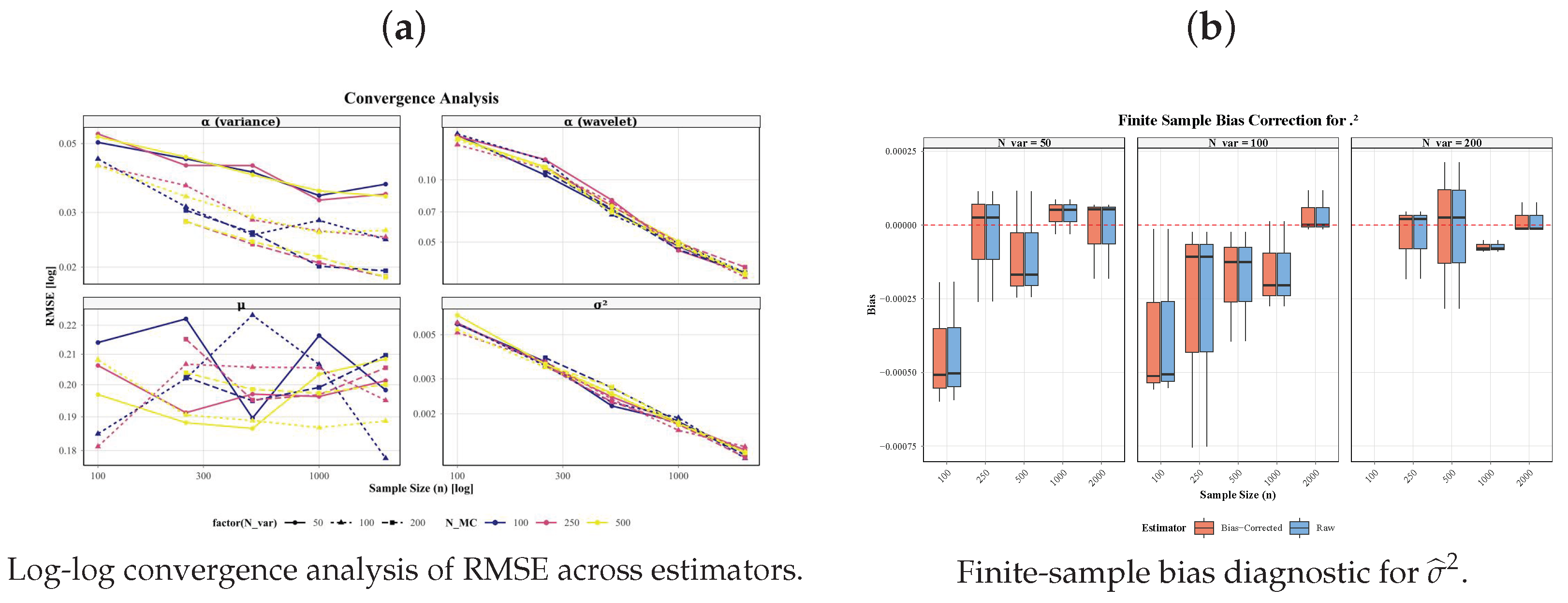
Figure 6 offers a more synthetic perspective. Panel (a) presents log–log convergence profiles of RMSE across estimators, enabling inspection of whether the empirical decay is at least broadly compatible with power-type stabilization, the natural language of rate comparison in fractional models. Panel (b) reports a finite-sample bias diagnostic for ${\displaystyle {\widehat{\sigma }}^2}$. This should be interpreted as an exploratory diagnostic rather than as a theorem-level correction formula; its function is to reveal the magnitude and direction of any remaining finite-sample distortion.

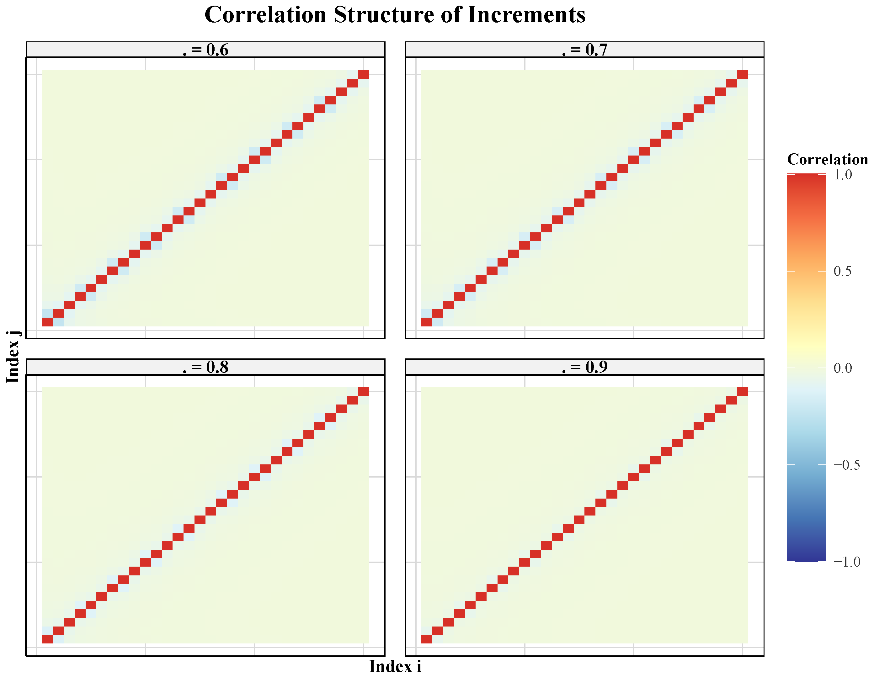
Finally, Figure 7 plays a structural role at least as important as the performance plots themselves. By displaying the correlation matrices of the increment process for several values of ${\displaystyle \alpha }$, it renders visible the manner in which the memory parameter reorganizes the entire dependence geometry. This visualization elucidates why both the semiparametric memory estimators and the Gaussian likelihood for ${\displaystyle (\mu ,{\sigma }^2)}$ are sensitive to the same underlying fractional mechanism, albeit through different statistical functionals.

5.9. Synthesis of the Numerical Evidence

Taken together, the tables and figures support a coherent and nuanced conclusion regarding the finite-sample behavior of inference procedures for Caputo fractional systems.

First, estimation of the memory parameter is intrinsically multi-regime. No single estimator dominates uniformly because the relevant statistical information enters through two fundamentally different channels. The variance-growth estimator is especially effective when independent path replication is available, its RMSE decreasing markedly with increasing ${\displaystyle N_{\mathrm{var}}}$. The wavelet-type estimator, by contrast, gains strength from fine temporal resolution along a single path, with RMSE improving systematically as ${\displaystyle n}$ increases. This complementarity is not accidental; it reflects two distinct projections of the same fractional mechanism onto different second-order summaries: the cross-sectional variance trajectory versus the multiscale increment contrasts.

Second, the oracle Gaussian likelihood analysis for ${\displaystyle (\mu ,{\sigma }^2)}$ exhibits differentiated but ultimately reassuring behavior. Diffusion estimation is highly stable, nearly unbiased at the scale reported, and accompanied by satisfactory empirical coverage. Drift estimation is considerably harder in point-estimation terms, a finding entirely plausible in view of the relatively weak deterministic signal and the strongly dependent increment noise, yet the corresponding interval estimates remain reasonably well calibrated under the matched covariance specification, with only isolated instances of undercoverage in low-resolution settings.

Third, the covariance visualizations confirm that the memory parameter should not be regarded as a secondary nuisance feature. It reshapes the entire dependence architecture of the observed data and thereby governs both the behavior of semiparametric memory estimators and the geometry of Gaussian likelihood inference. The correlation matrices for different ${\displaystyle \alpha }$ values reveal the progressive emergence of more persistent dependence as ${\displaystyle \alpha }$ increases toward unity, providing intuitive confirmation of the mechanism underlying the estimators’ performance.

Fourth, the Monte Carlo evidence validates the inferential framework at the exact level at which it is studied: semiparametric recovery of the memory parameter together with oracle second-stage likelihood inference for the finite-dimensional coefficients under a covariance model matched to the implemented discretization. A full plug-in analysis, in which a first-stage estimator of ${\displaystyle \alpha }$ is inserted into the covariance matrix, would require a separate experiment propagating memory-estimation uncertainty through the parametric step, which is a natural direction for subsequent investigation.

In this sense, the present simulation study provides a structurally faithful validation of the proposed computational methodology. It demonstrates that practically reliable inference for Caputo fractional systems is attainable provided one respects the distinction between replication-driven and resolution-driven information and models the fractional covariance structure at the likelihood stage without artificial simplification. The results also identify the drift parameter as the most challenging component of the inference problem, a finding that may guide future methodological development toward improved drift estimation procedures in strongly dependent fractional environments.

6. Empirical Validation: Sector-Aware Analysis of the S&P 500 Panel

6.1. Data Description and Preprocessing

We elucidate the empirical properties of the proposed Caputo fractional stochastic differential equation (Caputo–FSDE) framework through systematic application to a publicly available panel of U.S. equities (Kaggle, all-stocks-5yr), comprising daily price observations over a synchronized multi-year horizon. Following rigorous quality filtering, each retained ticker is conceptualized as a distinct path realization, with trading dates constituting the discrete observation mesh. The resultant data architecture is inherently compatible with panel-based stochastic process analysis, wherein each asset furnishes a singular realization of a long-memory stochastic trajectory. For each constituent ticker, we construct the transformed signal as

$$X_i\left(t_k\right)=log{P}_i\left(t_k\right)-log{P}_i\left(t_1\right),i=1,\dots ,N,$$

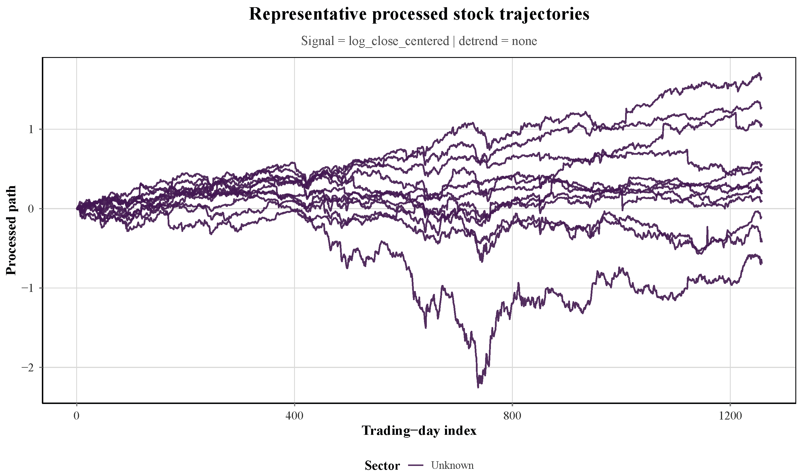
where ${\displaystyle P_i\left(t_k\right)}$ denotes the adjusted closing proxy at retained trading epoch ${\displaystyle t_k}$. In the baseline specification, we deliberately refrain from imposing deterministic detrending prior to estimation, thereby allowing the drift parameter to absorb systematic directional components inherent to the dynamics. Missing data are addressed through a two-stage protocol: initial filtering for common-date completeness, followed by linear interpolation of isolated residual gaps subsequent to temporal alignment. We provide an illustration of representative processed stock trajectories in Figure 8.

Beyond ticker-level inference, each retained asset is assigned to its corresponding economic sector contingent upon availability of constituent metadata. This sectoral annotation enables systematic investigation into whether the effective memory parameter and the Caputo–FSDE goodness-of-fit exhibit systematic variation across economically meaningful stratifications, see

Table 4. Global summary of the sector-aware Caputo–FSDE analysis on the all_stocks_5yr.csv panel. Each ticker is treated as one real trajectory observed on the common retained trading-day grid. The panel-wide memory parameter ${\displaystyle {\widehat{\alpha }}_{\mathrm{var}}}$ is estimated from the cross-sectional variance-growth relation, ticker-level ${\displaystyle {\widehat{\alpha }}_{\mathrm{wave}}}$ values are obtained by wavelet scaling, and ${\displaystyle (\widehat{\mu },{\widehat{\sigma }}^2)}$ are estimated via conditional Gaussian quasi-likelihood under the Caputo–FSDE covariance structure.

Parameter	Estimate	SD	Median	Q25	Q75	N
alpha_variance	0.990000	0.002331	0.990000	–	–	250
alpha_wavelet	0.942005	0.036120	0.942832	0.918962	0.970467	250
alpha_used_for_mle	0.990000	–	0.990000	–	–	250
mu_hat	0.000454	0.000472	0.000466	0.000195	0.000714	250
sigma2_hat	0.000261	0.000189	0.000216	0.000152	0.000318	250
delta_AIC	0.526387	0.768386	0.552137	0.014532	1.075318	250

.

6.2. Caputo–FSDE Specification

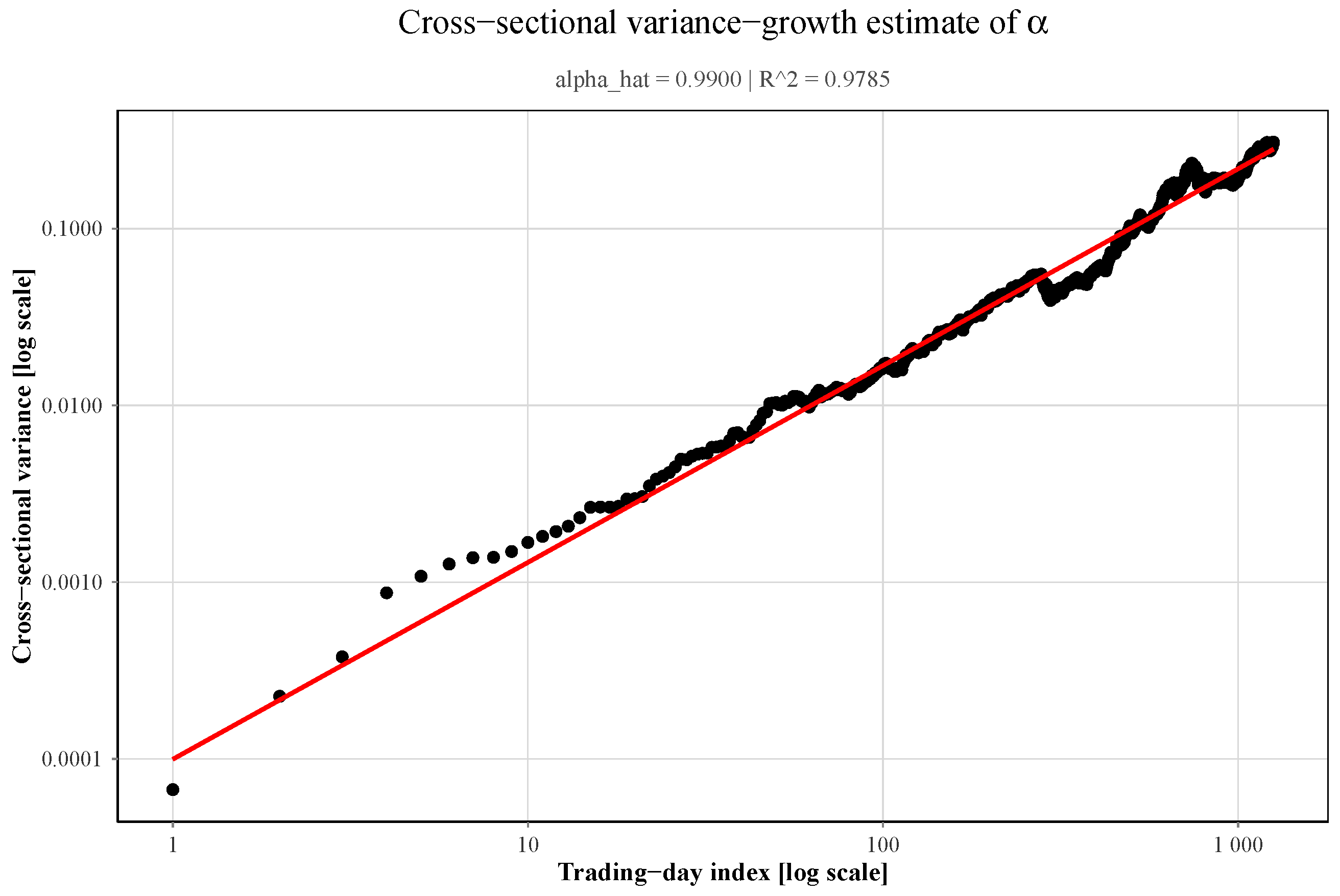
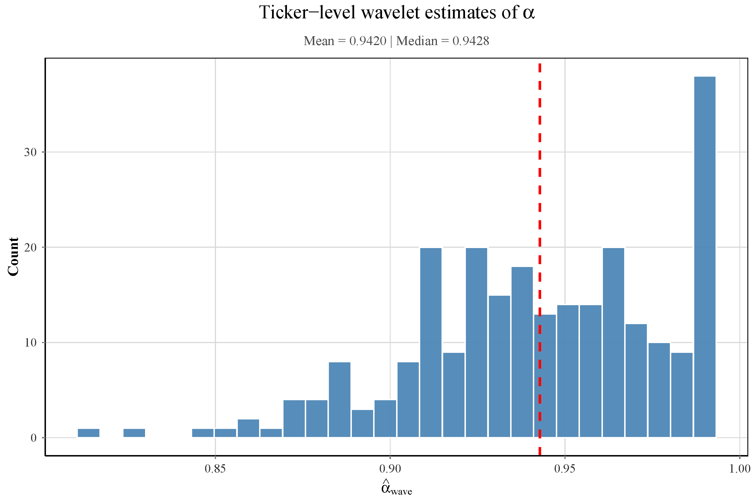
The empirical dynamics are characterized through a Caputo-type fractional stochastic differential representation, wherein the latent memory parameter ${\displaystyle \alpha \in (1/2,1)}$ jointly governs the variance scaling and the temporal dependence architecture of increments. At the panel level, we first recover the memory parameter via the cross-sectional variance-growth relation. Specifically, under correct specification, the cross-sectional dispersion of panel trajectories adheres asymptotically to a power law in time, with exponent identifying ${\displaystyle 2\alpha -1}$. This yields the global estimator ${\displaystyle {\widehat{\alpha }}_{\mathrm{var}}.}$ At the individual ticker level, we obtain a complementary estimate ${\displaystyle {\widehat{\alpha }}_{\mathrm{wave},i}}$ through wavelet-based scaling analysis, thereby providing a pathwise measure of memory heterogeneity across assets.

Conditional upon the selected memory parameter, drift and diffusion coefficients are estimated via Gaussian quasi-likelihood under the covariance structure induced by the Caputo–FSDE. This procedure generates ticker-specific estimators ${\displaystyle {\widehat{\mu }}_i}$ and ${\displaystyle {\widehat{\sigma }}_i^2}$, accompanied by residual-based adequacy diagnostics and information-theoretic comparisons against an iid Gaussian-increment benchmark.

6.3. Global Memory Estimation

Figure 9 depicts the log–log cross-sectional variance-growth relation computed from the balanced panel. The fitted slope yields the panel-wide estimate ${\displaystyle {\widehat{\alpha }}_{\mathrm{var}}}$, which synthesizes the average persistence structure across the equity universe. Given that the Brownian benchmark corresponds to the boundary value ${\displaystyle \alpha =1/2}$, empirical estimates significantly exceeding ${\displaystyle 1/2}$ provide compelling evidence of persistent dynamics and long-range dependence in the effective trajectories.

The cross-sectional estimate is complemented by the empirical distribution of ticker-level wavelet estimates, illustrated in Figure 10. This distribution illuminates whether memory phenomena are approximately homogeneous across assets or whether substantial cross-sectional heterogeneity underlies the panel average. In our framework, the comparison between ${\displaystyle {\widehat{\alpha }}_{\mathrm{var}}}$ and the empirical distribution of ${\displaystyle {\widehat{\alpha }}_{\mathrm{wave},i}}$ is particularly informative: close concordance suggests the global panel memory parameter is representative, whereas pronounced dispersion indicates heterogeneous persistence across assets.

6.4. Ticker-Level Inference and Model Comparison

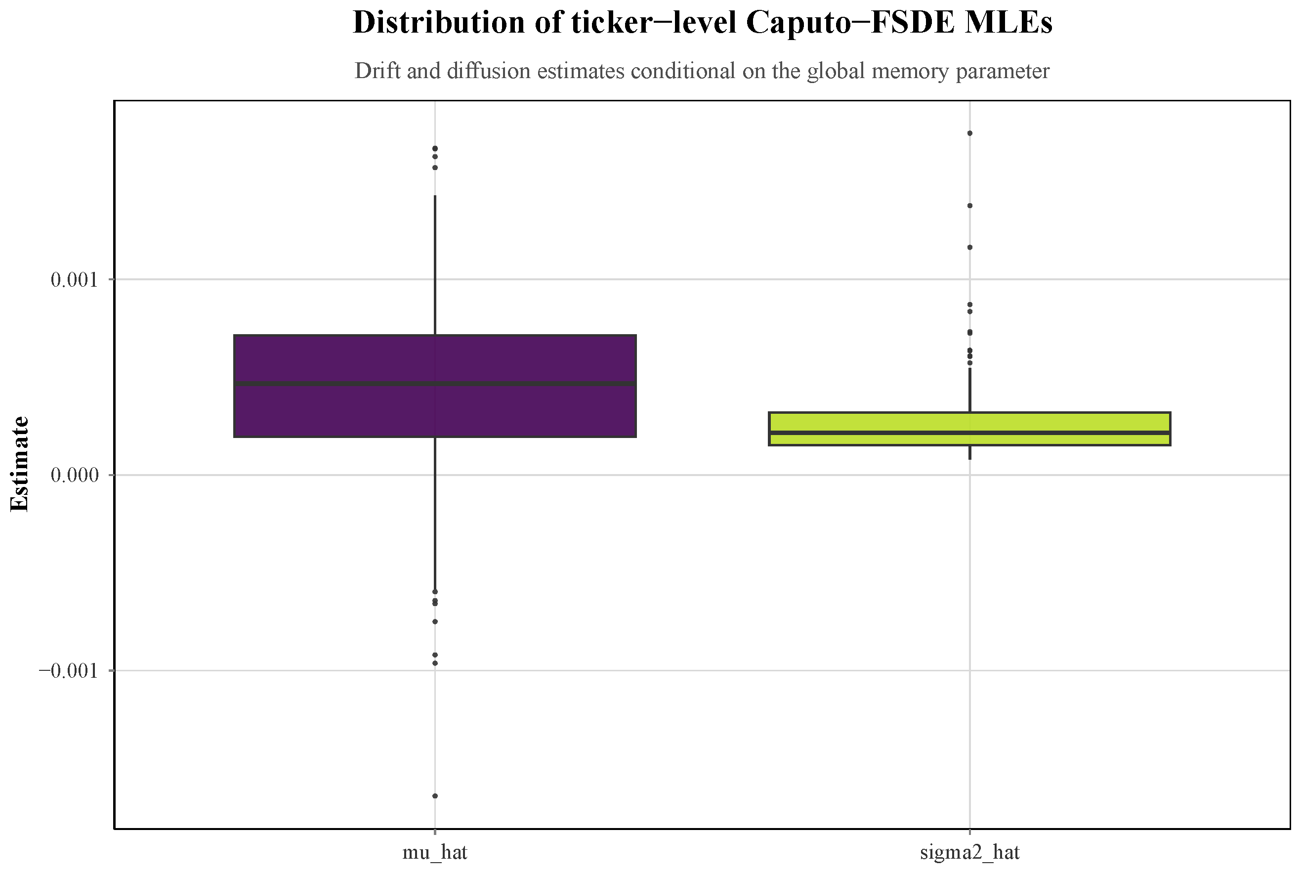
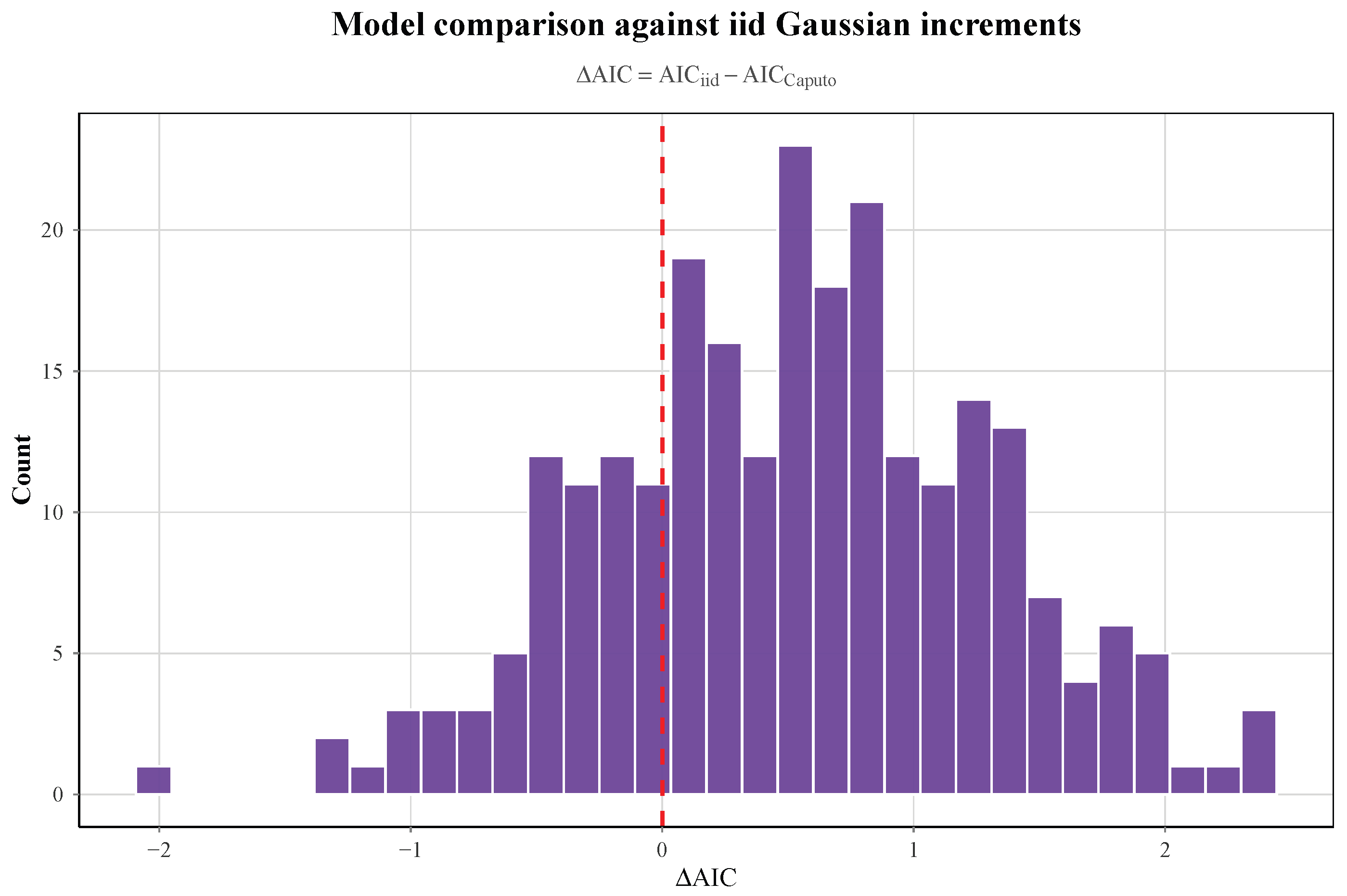
With the global memory parameter fixed for conditional likelihood estimation, we compute ticker-level estimates of drift and diffusion coefficients. The cross-sectional distributions of ${\displaystyle {\widehat{\mu }}_i}$ and ${\displaystyle {\widehat{\sigma }}_i^2}$ are presented in Figure 11. These estimates should not be interpreted as structural economic primitives in isolation; rather, they summarize the first-order directional component and second-order fluctuation scale implied by the fitted fractional model after accounting for memory structure. A central component of empirical validation involves comparing the Caputo–FSDE against a simpler iid Gaussian-increment benchmark. For each ticker, we compute

$$\mathrm{\Delta }AI{C}_i=AI{C}_{\mathrm{iid},i}-AI{C}_{\mathrm{Caputo},i},$$

such that positive values favor the Caputo–FSDE. The distribution of ${\displaystyle \mathrm{\Delta }AI{C}_i}$ provides a direct and interpretable measure of the frequency with which the long-memory formulation outperforms a memory-free alternative. Substantial positive values indicate that the fractional covariance structure captures aspects of the data generating process that cannot be replicated by independent Gaussian increments.

The best-performing tickers ranked by ${\displaystyle \mathrm{\Delta }AIC}$ are reported in

Table 5. Ticker-level ranking by information-criterion improvement over the iid Gaussian-increment benchmark. Positive values of ${\displaystyle \mathrm{\Delta }AIC=AI{C}_{\mathrm{iid}}-AI{C}_{\mathrm{Caputo}}}$ favor the Caputo–FSDE representation. The table highlights the strongest empirical support for long-memory dynamics together with residual adequacy diagnostics.

Ticker	Sector	${\displaystyle {\widehat{\mathit{\alpha }}}_{\mathbf{wave}}}$	${\displaystyle \widehat{\mathit{\mu }}}$	${\displaystyle {\widehat{\mathit{\sigma }}}^2}$	${\displaystyle \mathbf{\Delta }\mathit{AIC}}$	${\displaystyle {\mathit{p}}_{\mathit{JB}}}$	${\displaystyle {\mathit{p}}_{\mathit{LB}\left(10\right)}}$
COL	Unknown	0.9561	0.0007	0.000164	2.373	0.000	0.000
EFX	Unknown	0.9765	0.0006	0.000252	2.355	0.000	0.000
FIS	Unknown	0.9156	0.0008	0.000148	2.331	0.000	0.066
HIG	Unknown	0.9309	0.0007	0.000172	2.188	0.000	0.015
ECL	Unknown	0.9031	0.0005	0.000121	2.063	0.000	0.343
CRM	Unknown	0.9124	0.0008	0.000367	1.951	0.000	0.087
CL	Unknown	0.9125	0.0002	0.000102	1.940	0.000	0.019
EQT	Unknown	0.9485	${\displaystyle -}$0.0002	0.000415	1.931	0.000	0.007
HON	Unknown	0.8137	0.0006	0.000111	1.896	0.000	0.197
FLR	Unknown	0.9231	${\displaystyle -}$0.0001	0.000375	1.884	0.000	0.446
K	Unknown	0.9217	0.0001	0.000115	1.851	0.000	0.088
CTXS	Unknown	0.9139	0.0002	0.000329	1.849	0.000	0.003
EL	Unknown	0.9272	0.0006	0.000153	1.818	0.000	0.099
CTAS	Unknown	0.8810	0.0011	0.000126	1.816	0.000	0.398
AIG	Unknown	0.9100	0.0004	0.000173	1.801	0.000	0.121
BLL	Unknown	0.8579	0.0005	0.000162	1.786	0.000	0.647
BRK.B	Unknown	0.9510	0.0006	0.000087	1.718	0.000	0.122
IFF	Unknown	0.9260	0.0006	0.000151	1.683	0.000	0.058
HCA	Unknown	0.9329	0.0008	0.000279	1.668	0.000	0.338
AET	Unknown	0.8726	0.0011	0.000219	1.594	0.000	0.686

and completed by Figure 11 and Figure 12. These assets furnish the strongest empirical support for the proposed long-memory specification and constitute natural case studies for comprehensive residual diagnostics.

6.5. Sectoral Heterogeneity

A salient advantage of the panel structure resides in its capacity to examine whether memory characteristics and model adequacy vary across economically interpretable groupings. To this end, we aggregate ticker-level results by sector and recompute the cross-sectional variance-growth estimate within each sector conditional upon sufficient ticker availability. The resulting sector-specific summaries are tabulated in

Table 6. Sector-level summary of estimated memory and conditional dynamic parameters. For each retained economic sector, the table reports the sector-specific cross-sectional variance-growth estimate, the mean ticker-level wavelet estimate, mean drift and diffusion parameters, and the average information-criterion improvement relative to the iid Gaussian-increment benchmark.

Sector	Tickers	${\displaystyle {\widehat{\mathit{\alpha }}}_{\mathbf{var}}}$	${\displaystyle {\widehat{\mathit{\alpha }}}_{\mathbf{wave},\mathbf{mean}}}$	${\displaystyle {\widehat{\mathit{\mu }}}_{\mathbf{mean}}}$	${\displaystyle {\widehat{\mathit{\sigma }}}_{\mathbf{mean}}^2}$	${\displaystyle \mathbf{\Delta }{\mathit{AIC}}_{\mathbf{mean}}}$
Unknown	250	0.9900	0.9420	0.0005	0.000261	0.526

.

Several patterns merit scholarly attention. First, sectoral differentials in ${\displaystyle {\widehat{\alpha }}_{\mathrm{var}}}$ or in the average ${\displaystyle {\widehat{\alpha }}_{\mathrm{wave},i}}$ reveal that persistence is not uniform across economic activities. Second, variation in average ${\displaystyle \mathrm{\Delta }AIC}$ indicates that the empirical relevance of long-memory modeling is itself sector-dependent. Third, sector-specific pass rates of residual diagnostics offer an interpretable metric for assessing whether certain sectors are better characterized by the proposed specification than others.

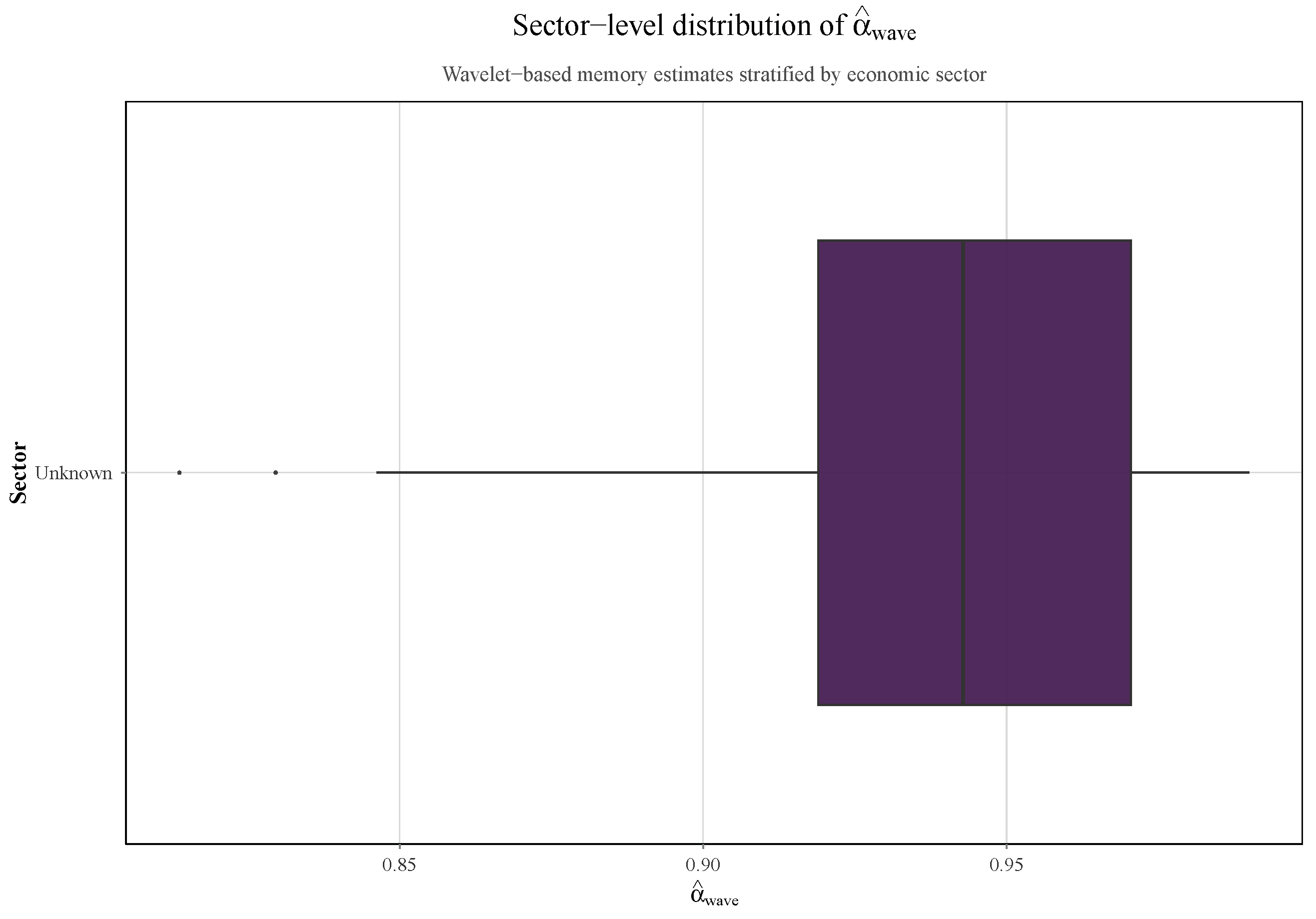
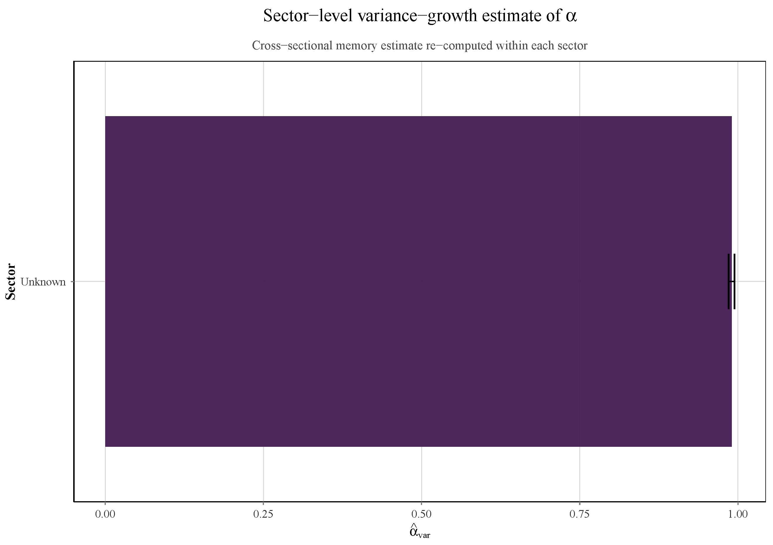
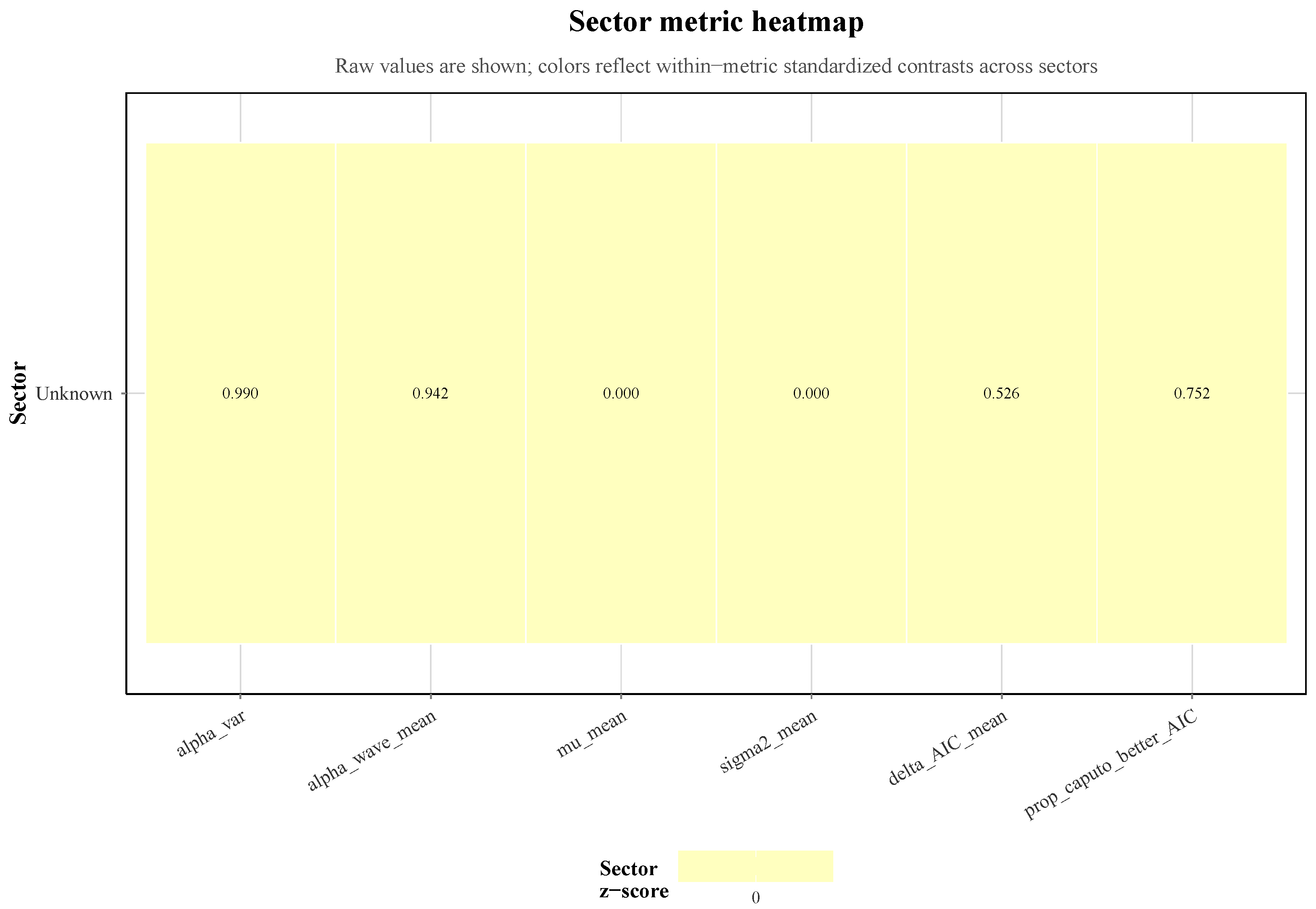
These cross-sector contrasts are visualized in Figure 13, Figure 14 and Figure 15. Collectively, these figures delineate three dimensions of heterogeneity: memory intensity, residual diffusion scale, and relative improvement over the iid benchmark.

6.6. Residual Adequacy and Representative Ticker Diagnostics

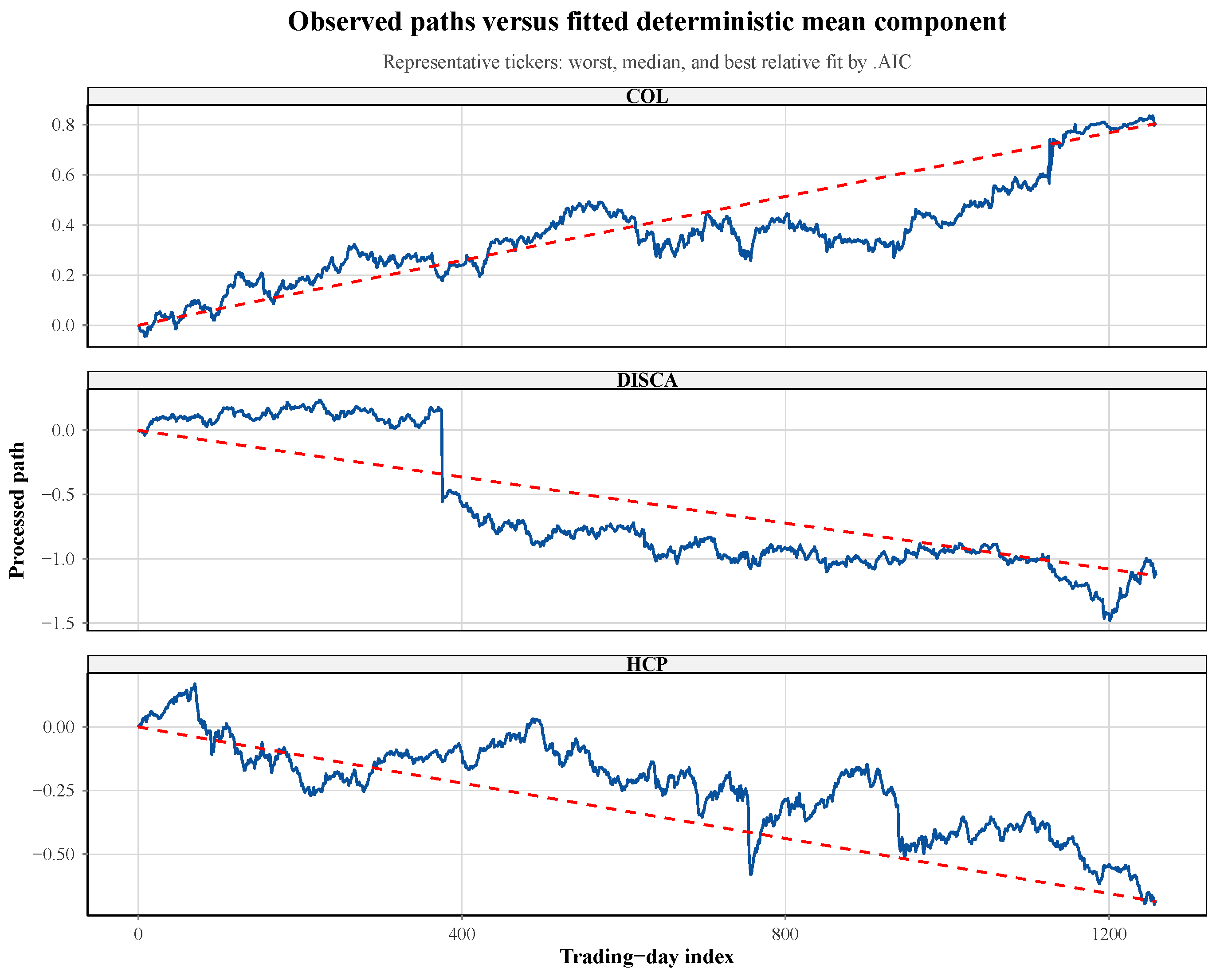
To scrutinize the adequacy of the fitted Caputo–FSDE model beyond information criteria, we examine representative tickers selected from the lower tail, center, and upper tail of the ${\displaystyle \mathrm{\Delta }AIC}$ distribution. These assets constitute a diagnostic triptych: a weakly supported case, a typical case, and a strongly supported case. For each representative ticker, Figure 16 juxtaposes the processed observed path with the fitted deterministic mean component. 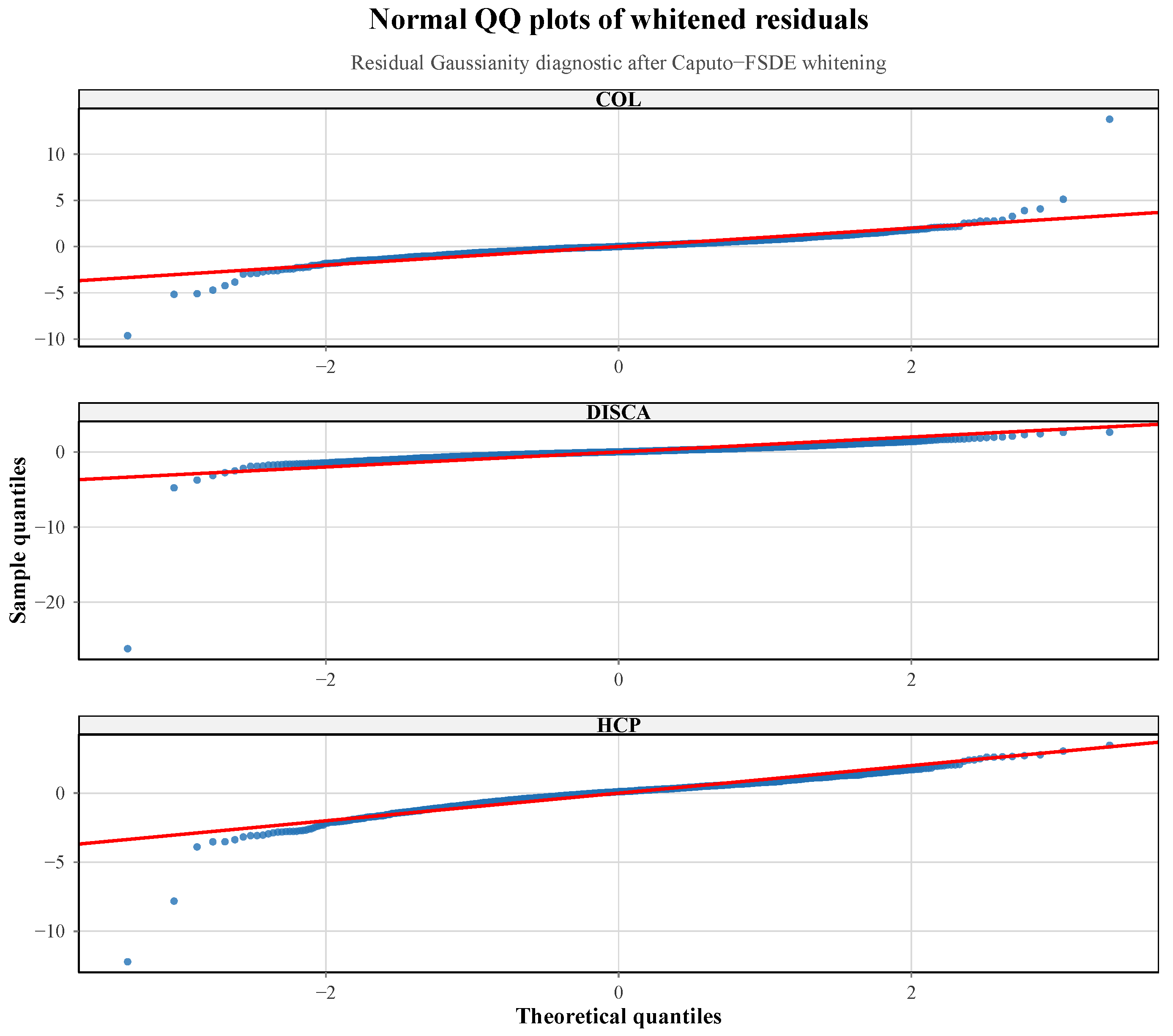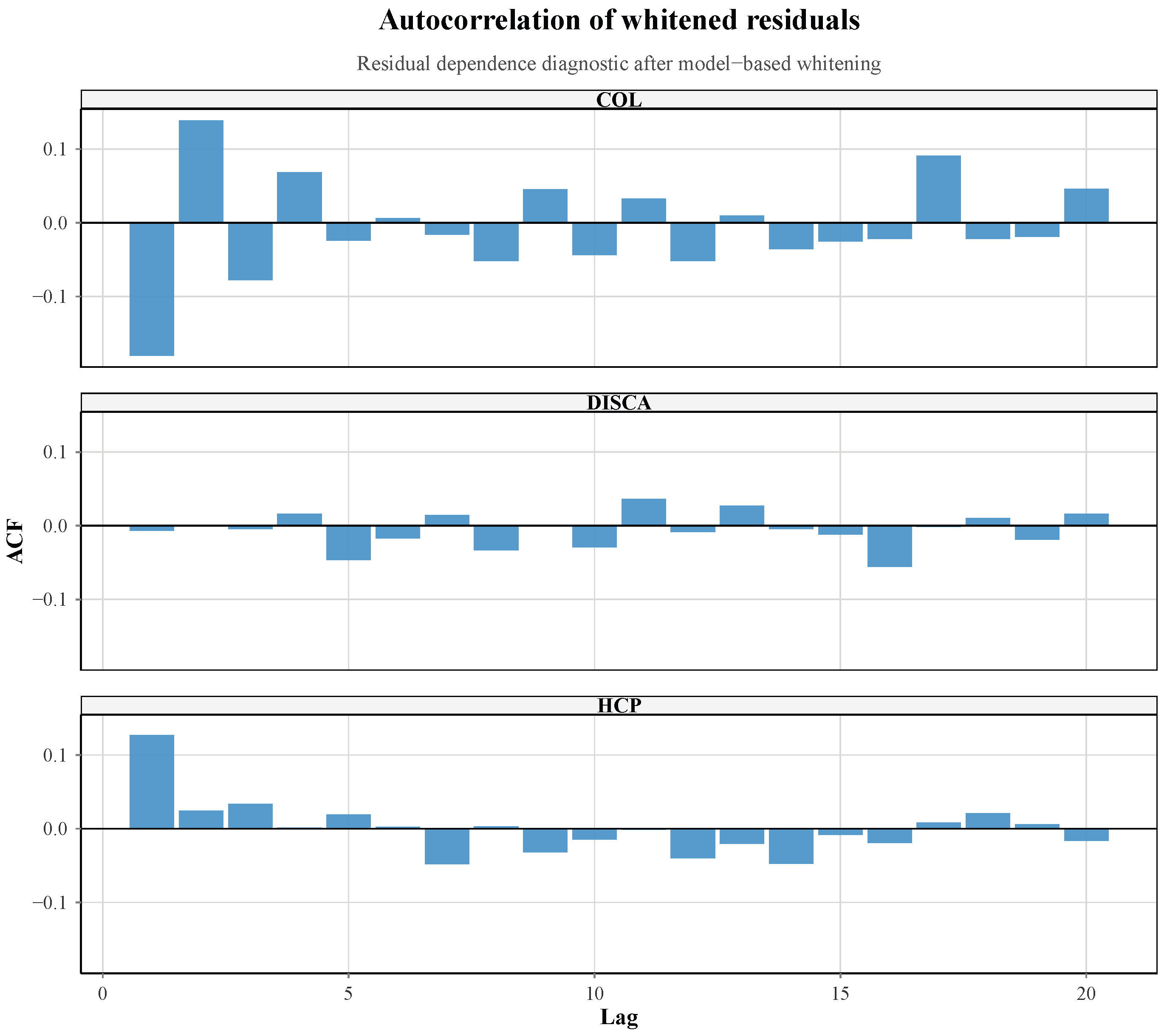Figure 17 and Figure 18 subsequently evaluate Gaussianity and residual serial dependence of the whitened residuals. Under ideal specification, QQ plots should remain proximal to the reference line, and residual autocorrelations should fluctuate around zero absent systematic structure. Deviations from these patterns indicate either heavy-tailed innovations, residual temporal dependence, or other forms of local misspecification, see

Table 7. Detailed diagnostic summary for representative tickers corresponding to the lower tail, median, and upper tail of the ${\displaystyle \mathrm{\Delta }AIC}$ distribution. These assets are used throughout the diagnostic figures to contrast poor, intermediate, and strong empirical agreement with the Caputo–FSDE specification.

Ticker	Sector	${\displaystyle {\widehat{\mathit{\alpha }}}_{\mathbf{wave}}}$	${\displaystyle \widehat{\mathit{\mu }}}$	${\displaystyle {\widehat{\mathit{\sigma }}}^2}$	Path RMSE	Inc. RMSE	${\displaystyle \mathbf{\Delta }\mathit{AIC}}$	${\displaystyle {\mathit{p}}_{\mathit{JB}}}$	${\displaystyle {\mathit{p}}_{\mathit{LB}\left(10\right)}}$
HCP	Unknown	0.9246	${\displaystyle -}$0.0006	0.000225	0.1488	0.0149	${\displaystyle -}$2.022	0.000	0.002
DISCA	Unknown	0.8874	${\displaystyle -}$0.0010	0.000733	0.2615	0.0269	0.546	0.000	0.790
COL	Unknown	0.9561	0.0007	0.000164	0.1184	0.0127	2.373	0.000	0.000

.

6.7. Local Memory Stability

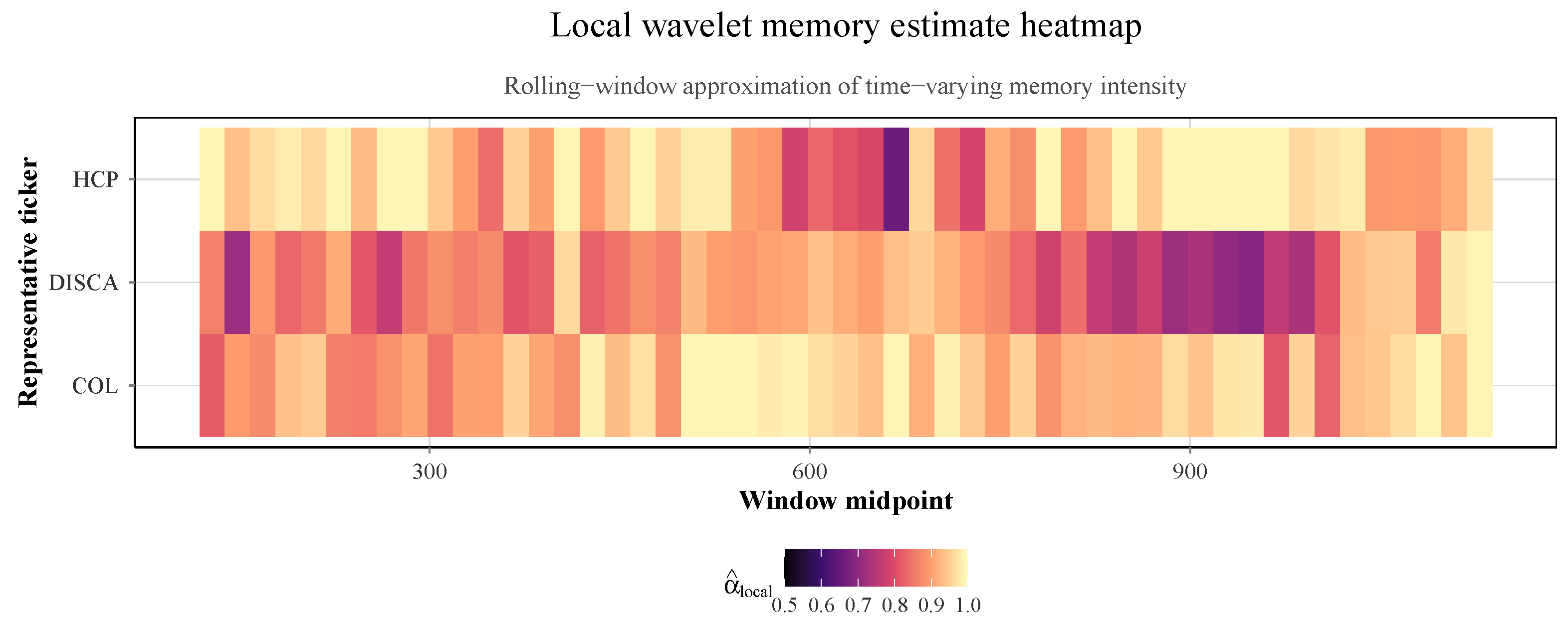
A single global memory parameter may prove unduly restrictive in the presence of nonstationarity or regime transitions. To investigate this possibility, we compute rolling wavelet estimates of the local memory parameter over moving windows. The resultant heatmap, displayed in Figure 19, provides a visual synopsis of time-varying persistence for the representative tickers.

This figure is particularly instrumental for discriminating between two qualitatively distinct scenarios. If the local memory index remains approximately stable over time, the global Caputo–FSDE approximation is structurally coherent. Conversely, pronounced temporal variation in local estimates suggests that a richer model—incorporating time-varying memory, structural breaks, or local re-estimation—may be necessitated.

6.8. Empirical Interpretation

Synthesizing the empirical evidence, three principal conclusions emerge. First, the panel exhibits nontrivial persistent dependence, as evidenced by the global variance-growth estimate and the distribution of ticker-level wavelet exponents. Second, information-criterion comparisons demonstrate that the Caputo–FSDE frequently dominates the iid Gaussian-increment benchmark, confirming that memory is not merely a visual artifact of trajectory geometry. Third, the magnitude and stability of estimated memory effects vary across sectors, indicating that persistence is not homogeneous across the equity universe.

From a modeling perspective, these findings suggest that the Caputo–FSDE provides a useful intermediate description between overly restrictive short-memory diffusions and fully nonparametric dependence structures. Simultaneously, residual and local-memory diagnostics reveal that a single global specification is not uniformly optimal across all assets. This observation naturally motivates future extensions involving sector-specific calibration, hierarchical memory pooling, or time-varying fractional parameters.

6.9. Concluding Remarks on the Real-Data

The real-data application demonstrates that the proposed methodology is operational on large financial panels and yields interpretable estimates of both long-memory intensity and conditional stochastic variability. Beyond parameter estimation, the integration of panel-based scaling, ticker-level wavelet diagnostics, conditional likelihood inference, and sector-aware model comparison offers a coherent framework for assessing whether fractional dynamics provide statistically meaningful improvements over simpler benchmarks in actual markets.

The sector-aware empirical analysis confirms that the proposed Caputo–FSDE methodology is not confined to stylized simulations. It can be implemented on large, unbalanced financial panels, transformed into a common-grid trajectory ensemble, and used to produce interpretable panel-wide, sector-level, and asset-specific measures of persistence. This renders the framework particularly attractive for applications wherein long-memory behavior is anticipated to be heterogeneous across economically structured stratifications.

7. Concluding Remarks and Perspectives

This paper develops a unified inference framework for a Gaussian white-noise driven dynamical system governed by a Caputo fractional derivative. Starting from the Volterra representation of the solution, we make explicit how the fractional order ${\displaystyle \alpha }$ reshapes the probabilistic structure of the model: it alters the scaling of fluctuations, induces long-range dependence through a non-local kernel, and produces correlated increments that fall outside the standard semimartingale paradigm. On this basis, we propose and analyze complementary statistical procedures for recovering the triplet of structural parameters ${\displaystyle (\alpha ,\mu ,{\sigma }^2)}$ from discretely observed data. In particular, the variance-growth approach and the wavelet scaling method provide two principled routes for estimating ${\displaystyle \alpha }$, while a Gaussian pseudo-likelihood built from the increment vector yields closed-form estimators for ${\displaystyle (\mu ,{\sigma }^2)}$. Beyond consistency and central limit theorems, the availability of Berry–Esseen type bounds offers quantitative control of Gaussian approximation errors, which is essential for rigorous uncertainty quantification in finite samples.

Theoretical significance. From a methodological viewpoint, the results contribute to the growing statistical theory for fractional stochastic systems by highlighting a tractable “Gaussian–Volterra + fractional calculus” interface. The explicit covariance structure of the increments, together with Malliavin calculus tools, makes it possible to go beyond asymptotic normality and to derive distributional approximations with rates. Such quantitative results are particularly valuable in long-memory settings, where classical weak convergence arguments often provide limited guidance for practical sample sizes. The framework also clarifies the role of ${\displaystyle \alpha }$ as a simultaneous memory and regularity index: it governs both the small-time variance scaling and the strength of dependence across increments, thereby affecting identifiability, estimator efficiency, and the geometry of the likelihood surface.

Applied relevance. The model studied here is a parsimonious yet expressive prototype for phenomena with persistent memory and anomalous diffusion. In quantitative finance, it can be viewed as a stylized building block for volatility or factor dynamics exhibiting long memory; in physics and engineering, it relates to viscoelasticity and transport with hereditary effects; and in biology or epidemiology, it offers a compact mechanism to encode lagged responses and cumulative exposure. In each of these domains, the fractional order ${\displaystyle \alpha }$ is not merely a nuisance parameter but a scientifically interpretable quantity that modulates persistence and smoothness. The simulation evidence reported in this work supports the practical viability of the proposed estimators and confirms that confidence intervals based on asymptotic theory can achieve near-nominal coverage in realistically sized experiments.

Perspectives: statistical theory. Several theoretical directions emerge naturally.

(i)

Joint inference and plug-in effects. While the present study analyzes estimators of ${\displaystyle \alpha }$ and of ${\displaystyle (\mu ,{\sigma }^2)}$ in a largely modular fashion, an important extension is a fully joint analysis of ${\displaystyle (\widehat{\alpha },\widehat{\mu },{\widehat{\sigma }}^2)}$, including the propagation of uncertainty from ${\displaystyle \widehat{\alpha }}$ into the pseudo–MLE step. Establishing stable plug-in central limit theorems and deriving second-order expansions for the joint law would strengthen the foundations of simultaneous inference.

(ii)

Optimality and efficiency bounds. A deeper understanding of information content in fractional Volterra models calls for Cramér–Rao type lower bounds and semiparametric efficiency analyses. In particular, it would be valuable to characterize regimes (considering ${\displaystyle T}$ fixed and ${\displaystyle \mathrm{\Delta }t\to 0}$, or ${\displaystyle T\to \infty }$) where ${\displaystyle \alpha }$ is estimable at parametric rate, and to identify efficient estimating equations that exploit the full dependence structure of the increments.

(iii)

High-frequency asymptotics under dependence and irregular sampling. The current setting relies on a regular grid. Extending the theory to irregular designs, missing observations, asynchronous sampling, or microstructure-type perturbations is of direct practical interest. In such contexts, the covariance structure becomes more intricate and robust procedures (e.g., pre-averaging, subsampling, or debiasing) may be required.

(iv)

Model enrichment: non-constant coefficients and non-Gaussian driving noise. Allowing ${\displaystyle (\mu ,\sigma )}$ to vary in time or state, or replacing Gaussian white noise by non-Gaussian innovations (e.g., Lévy noise or Hermite-type inputs), would broaden applicability. These generalizations raise nontrivial identifiability and approximation issues, and would require new Malliavin/Stein arguments or alternative normal approximation tools.

(v)

Non-asymptotic and finite-sample guarantees. While Berry–Esseen bounds provide quantitative asymptotics, an ambitious direction is to obtain sharper non-asymptotic risk bounds (oracle inequalities, concentration inequalities for dependent Gaussian quadratic forms, and finite-sample confidence regions) tailored to fractional covariance operators.

Perspectives: computation and large-scale implementation. Fractional models often come with computational bottlenecks due to dense covariance matrices. Two important avenues are: (i) the development of fast linear algebra for Toeplitz-like or kernel-induced matrices (circulant embedding, FFT-based solvers, hierarchical matrices), and (ii) scalable likelihood approximations (Whittle-type frequency-domain likelihoods, composite likelihoods, or low-rank kernel approximations) that preserve statistical efficiency while reducing complexity.

Perspectives: machine learning and data-driven fractional inference. The interaction between fractional stochastic modeling and modern machine learning is particularly promising.

(i)

Physics-informed learning for fractional dynamics. One can embed the Caputo operator and the Volterra representation into physics-informed neural networks (PINNs) or operator-learning architectures, enforcing the fractional dynamics as a soft constraint. This is appealing when data are sparse or partially observed, and when the goal is to learn latent trajectories together with ${\displaystyle (\alpha ,\mu ,{\sigma }^2)}$.

(ii)

Neural surrogates for likelihoods and covariance operators. Likelihood-based inference can be accelerated by learning surrogates for expensive objects (e.g., mapping ${\displaystyle \alpha \mapsto A{\left(\alpha \right)}^{-1}b}$ or ${\displaystyle log\left|A\right(\alpha \left)\right|}$) using amortized inference, normalizing flows, or neural operators. Such surrogates can enable near-real-time estimation in high-frequency settings and facilitate Bayesian workflows.

(iii)

Simulation-based inference (SBI). Since the model admits efficient simulation via Volterra discretizations, it is natural to consider likelihood-free approaches (neural posterior estimation, neural ratio estimation) that learn the posterior of ${\displaystyle (\alpha ,\mu ,{\sigma }^2)}$ from summary statistics or from raw paths. A key research question is to design summaries that are informative for long-memory structure (multi-scale wavelet energies, periodogram-based features, or quadratic forms matched to the covariance kernel).

(iv)

Robust and adaptive multi-scale estimators. Machine learning can be used to adaptively choose scales in the wavelet regression, select optimal design points for variance-growth estimation, or combine estimators via stacking to minimize predictive risk. Such adaptive procedures could improve robustness under contamination, nonstationarities, or mild misspecification.

(v)

Learning fractional order as a functional parameter. In complex systems, the effective memory exponent may vary over time (multifractional behavior). Extending the present framework to estimate a time-varying order ${\displaystyle \alpha \left(t\right)}$ suggests a hybrid of statistical regularization (e.g., total variation or Sobolev penalties) and ML-based representation learning, with applications to regime changes and evolving persistence.

Outlook: Overall, the present work demonstrates that fractional stochastic dynamics can be brought into a rigorous inference framework that is both analytically tractable and empirically effective. The combination of explicit Volterra structure, Malliavin-based distributional approximation, and multi-scale estimation techniques offers a versatile methodological toolkit. We anticipate that extending these ideas to richer fractional systems—including non-linear coefficients, multivariate settings, and data-imperfect regimes—and integrating them with modern simulation-based and physics-informed learning paradigms will substantially expand the scope of statistically principled fractional modeling in the applied sciences.

8. Proofs

This section is devoted to the proofs of our results. The notation introduced earlier continues to be used throughout.

8.1. Proof of Proposition 1

(a) 

By applying the Caputo fractional integral to Equation (4), we obtain:

$$\begin{array}{c}\hfill X_t=X_0+{\displaystyle \frac{\mu t^{\alpha }}{\alpha \mathrm{\Gamma }\left(\alpha \right)}}+{\displaystyle \frac{\sigma }{\mathrm{\Gamma }\left(\alpha \right)}}{\int }_0^t{(t-s)}^{\alpha -1}d{B}_s.\end{array}$$

(b) 

It is straightforward to verify that, for every ${\displaystyle t>0}$,

$${\int }_0^t{(t-s)}^{2(\alpha -1)}ds={\displaystyle \frac{t^{2\alpha -1}}{2\alpha -1}}<\infty ,$$

provided that ${\displaystyle \alpha >\frac{1}{2}}$. Hence, the kernel ${\displaystyle s\mapsto {(t-s)}^{\alpha -1}}$ belongs to ${\displaystyle L^2\left([0,t]\right)}$ and, therefore, the stochastic convolution

$${\int }_0^t{(t-s)}^{\alpha -1}d{B}_s$$

is well defined in the Itô sense. By the standard properties of Wiener integrals, this term is a centered Gaussian random variable. It follows from the explicit representation (5) that ${\displaystyle {\left(X_t\right)}_{t\ge 0}}$ is a Gaussian process.

We now determine the first two moments of ${\displaystyle X_t}$. Taking expectations in (5) yields

$$\mathbb{E}\left(X_t\right)={\displaystyle \frac{\mu }{\alpha \mathrm{\Gamma }\left(\alpha \right)}}{t}^{\alpha }+\mathbb{E}\left(X_0\right).$$

(71)

Next, assuming that ${\displaystyle X_0}$ is independent of the driving Brownian motion ${\displaystyle B}$, we compute the variance directly from the explicit form of the solution:

$$X_t=X_0+{\displaystyle \frac{\mu }{\alpha \mathrm{\Gamma }\left(\alpha \right)}}{t}^{\alpha }+{\displaystyle \frac{\sigma }{\mathrm{\Gamma }\left(\alpha \right)}}{\int }_0^t{(t-s)}^{\alpha -1}d{B}_s.$$

Since the deterministic drift does not contribute to the variance, and since the Wiener integral is centered and independent of ${\displaystyle X_0}$, we obtain

$$\begin{array}{cc}\hfill \mathrm{Var}\left(X_t\right)& =\mathrm{Var}\left(X_0\right)+{\displaystyle \frac{{\sigma }^2}{{\mathrm{\Gamma }}^2\left(\alpha \right)}}\mathrm{Var}\left({\int }_0^t{(t-s)}^{\alpha -1}d{B}_s\right).\hfill \end{array}$$

Applying the Itô isometry, we deduce that

$$\begin{array}{cc}\hfill \mathrm{Var}\left(X_t\right)& =\mathrm{Var}\left(X_0\right)+{\displaystyle \frac{{\sigma }^2}{{\mathrm{\Gamma }}^2\left(\alpha \right)}}{\int }_0^t{(t-s)}^{2\alpha -2}ds\hfill \\ \hfill & =\mathrm{Var}\left(X_0\right)+{\displaystyle \frac{{\sigma }^2}{{\mathrm{\Gamma }}^2\left(\alpha \right)}}·{\displaystyle \frac{t^{2\alpha -1}}{2\alpha -1}}.\hfill \end{array}$$

Therefore,

$$\mathrm{Var}\left(X_t\right)=\mathrm{Var}\left(X_0\right)+{\displaystyle \frac{{\sigma }^2}{(2\alpha -1){\mathrm{\Gamma }}^2\left(\alpha \right)}}{t}^{2\alpha -1}.$$

Hence the proof is complete.

8.2. Proof of Proposition 2

We have

$$\begin{array}{ccc}\hfill \mathrm{Cov}(X_{t+\delta },X_t)& =& \mathbb{E}\left(X_{t+\delta }{X}_t\right)-\mathbb{E}\left(X_t\right)\mathbb{E}\left(X_{t+\delta }\right).\hfill \end{array}$$

From Equation (5), we get

$$X_{t+\delta }=X_0+{\displaystyle \frac{\mu {(t+\delta )}^{\alpha }}{\alpha \mathrm{\Gamma }\left(\alpha \right)}}+{\displaystyle \frac{\sigma }{\mathrm{\Gamma }\left(\alpha \right)}}{\int }_0^{t+\delta }{(t+\delta -s)}^{\alpha -1}d{B}_s.$$

We readily obtain

$$\begin{array}{ccc}\hfill \mathbb{E}\left(X_t{X}_{t+\delta }\right)& =& \mathbb{E}\left(X_0^2\right)+\mathbb{E}\left(X_0\right){\displaystyle \frac{\mu {(t+\delta )}^{\alpha }}{\alpha \mathrm{\Gamma }\left(\alpha \right)}}+\mathbb{E}\left(X_0\right){\displaystyle \frac{\mu t^{\alpha }}{\alpha \mathrm{\Gamma }\left(\alpha \right)}}+{\displaystyle \frac{{\mu }^2}{{\alpha }^2{\mathrm{\Gamma }}^2\left(\alpha \right)}}{t}^{\alpha }{(t+\delta )}^{\alpha }\hfill \\ & & +{\displaystyle \frac{{\sigma }^2}{{\mathrm{\Gamma }}^2\left(\alpha \right)}}{\int }_0^t{\left[(t-s)(t+\delta -s)\right]}^{\alpha -1}ds.\hfill \end{array}$$

Then

$$\begin{array}{ccc}\hfill \mathrm{Cov}(X_{t+\delta },X_t)& =& Var\left(X_0\right)+{\displaystyle \frac{{\sigma }^2}{{\mathrm{\Gamma }}^2\left(\alpha \right)}}{\int }_0^t{\left[(t-s)(t+\delta -s)\right]}^{\alpha -1}ds.\hfill \end{array}$$

8.3. Proof of Theorem 1

Lemma 1.

Let ${\displaystyle {\widehat{V}}_n\left(t_j\right)}$ be the unbiased variance estimator defined in (12). Then, for any ${\displaystyle j,k\in \{1,\dots ,m\}}$, the covariance between the estimators ${\displaystyle {\widehat{V}}_n\left(t_j\right)}$ and ${\displaystyle {\widehat{V}}_n\left(t_k\right)}$ admits the closed-form expression

$$\mathrm{Cov}\left({\widehat{V}}_n\left(t_j\right),{\widehat{V}}_n\left(t_k\right)\right)={\displaystyle \frac{2}{n-1}}{\mathrm{Cov}}^2\left(X_{t_j},X_{t_k}\right).$$

(72)

Moreover, the covariance structure of the underlying process is given explicitly by

$$\mathrm{Cov}(X_{t_j},X_{t_k})={\displaystyle \frac{{\sigma }^2}{{\mathrm{\Gamma }}^2\left(\alpha \right)}}{\int }_0^{min(t_j,t_k)}{\left((t_j-u)(t_k-u)\right)}^{\alpha -1}\mathrm{d}u,$$

where ${\displaystyle \mathrm{\Gamma }(·)}$ denotes the Euler gamma function and ${\displaystyle {\sigma }^2>0}$ is the scale parameter of the model.

(i) 

Unbiasedness and ${\displaystyle {\mathit{L}}^{\mathbf{2}}}$–convergence of the estimator ${\displaystyle \widehat{\mathit{\alpha }}}$:

We start with the linear regression model

$$y_j={\beta }_0+{\beta }_1{x}_j+{\epsilon }_j,$$

where

$$y_j=log{\widehat{V}}_n\left(t_j\right),x_j=log{t}_j,{\beta }_1:=2\alpha -1,{\beta }_0:=log{C}_{\alpha ,\sigma }.$$

Taking averages, we obtain

$$\begin{array}{ccc}\hfill \overline{y}& =& {\displaystyle \frac{1}{m}}\sum _{j=1}^m{y}_j={\displaystyle \frac{1}{m}}\sum _{j=1}^m({\beta }_0+{\beta }_1{x}_j+{\epsilon }_j)={\beta }_0+{\beta }_1\overline{x}+\overline{\epsilon }.\hfill \end{array}$$

(73)

Subtracting the mean from each observation yields

$$\begin{array}{c}\hfill y_j-\overline{y}={\beta }_1(x_j-\overline{x})+({\epsilon }_j-\overline{\epsilon }).\end{array}$$

(74)

Consequently, the least squares estimator of ${\displaystyle {\beta }_1}$ is

$$\begin{array}{ccc}\hfill \widehat{{\beta }_1}& =& {\displaystyle \frac{{\displaystyle \sum _{j=1}^m(x_j-\overline{x})(y_j-\overline{y})}}{{\displaystyle \sum _{j=1}^m{(x_j-\overline{x})}^2}}}={\beta }_1+{\displaystyle \frac{{\displaystyle \sum _{j=1}^m(x_j-\overline{x}){\epsilon }_j}}{{\displaystyle \sum _{j=1}^m{(x_j-\overline{x})}^2}}}.\hfill \end{array}$$

Then,

$$\widehat{{\beta }_1}={\beta }_1+{\displaystyle \frac{{\displaystyle \sum _{j=1}^m(log{t}_j-\overline{logt}){\epsilon }_j}}{{\displaystyle \sum _{j=1}^m{(log{t}_j-\overline{logt})}^2}}}.$$

(75)

Taking expectations, we have

$$\mathbb{E}\left(\widehat{{\beta }_1}\right)={\beta }_1+{\displaystyle \frac{{\displaystyle \sum _{j=1}^m(log{t}_j-\overline{logt})\mathbb{E}\left({\epsilon }_j\right)}}{{\displaystyle \sum _{j=1}^m{(log{t}_j-\overline{logt})}^2}}}.$$

(76)

Since ${\displaystyle {\widehat{V}}_n\left(t_j\right)}$ is an unbiased estimator of ${\displaystyle \mathbb{V}ar\left(X_{t_j}\right)}$, we get

$$\mathbb{E}\left({\epsilon }_j\right)={\displaystyle \frac{\mathbb{E}\left({\widehat{V}}_n\left(t_j\right)\right)-\mathbb{V}ar\left(X_{t_j}\right)}{\mathbb{V}ar\left(X_{t_j}\right)}}=0.$$

we deduce that,

$$\mathbb{E}\left(\widehat{{\beta }_1}\right)={\beta }_1.$$

(77)

Finally, since ${\displaystyle \alpha =\frac{1}{2}({\beta }_1+1)}$, it follows that

$$\mathbb{E}\left({\widehat{\alpha }}_n\right)={\displaystyle \frac{1}{2}}(\mathbb{E}\left(\widehat{{\beta }_1}\right)+1)={\displaystyle \frac{1}{2}}({\beta }_1+1)=\alpha .$$

(78)

Therefore, we conclude that ${\displaystyle {\widehat{\alpha }}_n}$ is an unbiased estimator of ${\displaystyle \alpha }$. Second, by (75) we get

$$\begin{array}{c}\hfill \mathbb{E}{(\widehat{{\beta }_1}-{\beta }_1)}^2={\displaystyle \frac{{\displaystyle \sum _{j=1}^m\sum _{k=1}^m(log{t}_j-\overline{logt})(log{t}_k-\overline{logt})\mathbb{E}\left({\epsilon }_j{\epsilon }_k\right)}}{{\displaystyle {\left(\sum _{j=1}^m{(log{t}_j-\overline{logt})}^2\right)}^2}}}.\end{array}$$

(79)

Note

$$\begin{array}{ccc}\hfill \mathbb{E}\left({\epsilon }_j{\epsilon }_k\right)& =& \mathbb{E}\left[\left({\displaystyle \frac{{\widehat{V}}_n\left(t_j\right)-\mathbb{V}ar\left(X_{t_j}\right)}{\mathbb{V}ar\left(X_{t_j}\right)}}\right)\left({\displaystyle \frac{{\widehat{V}}_n\left(t_k\right)-\mathbb{V}ar\left(X_{t_k}\right)}{\mathbb{V}ar\left(X_{t_k}\right)}}\right)\right]\hfill \\ & =& {\displaystyle \frac{\mathbb{C}ov\left({\widehat{V}}_n\left(t_j\right),{\widehat{V}}_n\left(t_k\right)\right)}{\mathbb{V}ar\left(X_{t_j}\right)\mathbb{V}ar\left(X_{t_k}\right)}}.\hfill \end{array}$$

(80)

By Lemma (1), (7) and (8), we have

$$\begin{array}{ccc}\hfill \mathbb{E}\left({\epsilon }_j{\epsilon }_k\right)& =& {\displaystyle \frac{2}{n-1}}·{\displaystyle \frac{Co{v}^2\left(X_{t_j},X_{t_k}\right)}{\mathbb{V}ar\left(X_{t_j}\right)\mathbb{V}ar\left(X_{t_k}\right)}}\hfill \\ & =& {\displaystyle \frac{2}{n-1}}·{\displaystyle \frac{{\left(2\alpha -1\right)}^2}{{\left(t_j{t}_k\right)}^2}}{\left({\int }_0^{min(t_j,t_k)}{\left((t_j-u)(t_k-u)\right)}^{\alpha -1}\mathrm{d}u\right)}^2;\hfill \end{array}$$

which yields

$$\begin{array}{c}\hfill \mathbb{E}\left({\epsilon }_j{\epsilon }_k\right)⟶0\mathrm{as}n⟶\infty .\end{array}$$

(81)

Hence, by (79) and (81), we get

$$\mathbb{E}{(\widehat{{\beta }_1}-{\beta }_1)}^2⟶0\mathrm{as}n⟶\infty .$$

(82)

This implies that

$$\mathbb{E}{({\widehat{\alpha }}_n-\alpha )}^2⟶0\mathrm{as}n⟶\infty .$$

(83)

(ii) 

Strong Consistency of the Estimator ${\displaystyle {\widehat{\alpha }}_n}$:

According to the Law of Large Numbers, each sample variance converges almost surely to the corresponding theoretical variance:

$${\widehat{V}}_n\left(t_j\right)\stackrel{a.s.}{\to }\mathbb{V}ar\left(X_{t_j}\right)=C_{\alpha ,\sigma }{t}_j^{2\alpha -1},\mathrm{as}n\to \infty .$$

(84)

Taking logarithms,

$$y_j=log{\widehat{V}}_n\left(t_j\right)\stackrel{a.s.}{\to }log{C}_{\alpha ,\sigma }+(2\alpha -1)log{t}_j={\beta }_0+{\beta }_1{x}_j.$$

(85)

Then,

$$\begin{array}{c}\hfill y_j-\overline{y}\stackrel{a.s.}{\to }{\beta }_1(x_j-\overline{x}).\end{array}$$

(86)

Consequently,

$$\begin{array}{ccc}\hfill \widehat{{\beta }_1}& =& {\displaystyle \frac{{\displaystyle \sum _{j=1}^m(x_j-\overline{x})(y_j-\overline{y})}}{{\displaystyle \sum _{j=1}^m{(x_j-\overline{x})}^2}}}\stackrel{a.s.}{\to }{\displaystyle \frac{{\displaystyle \sum _{j=1}^m(x_j-\overline{x})\left({\beta }_1(x_j-\overline{x})\right)}}{{\displaystyle \sum _{j=1}^m{(x_j-\overline{x})}^2}}}={\beta }_1.\hfill \end{array}$$

Since ${\displaystyle \alpha =\frac{1}{2}({\beta }_1+1)}$, it follows that

$$\begin{array}{c}\hfill {\widehat{\alpha }}_n\stackrel{a.s.}{\to }\alpha .\end{array}$$

(87)

(iii) 

Asymptotic normality of the estimator ${\displaystyle {\widehat{\mathit{\alpha }}}_{\mathit{n}}}$:

By (75), we recall that

$$\widehat{{\beta }_1}-{\beta }_1={\displaystyle \frac{{\displaystyle \sum _{j=1}^m(log{t}_j-\overline{logt}){\epsilon }_j}}{{\displaystyle \sum _{j=1}^m{(log{t}_j-\overline{logt})}^2}}};$$

with

$${\epsilon }_j=log{\widehat{V}}_n\left(t_j\right)-log\mathbb{V}ar\left(X_{t_j}\right).$$

(88)

8.3.1. Asymptotic Normality of the Variance Estimator

Let

$${\widehat{V}}_n\left(t_j\right)={\displaystyle \frac{1}{n-1}}\sum _{i=1}^n{\left(X_{t_j}^{\left(i\right)}-{\overline{X}}_{t_j}\right)}^2,{\overline{X}}_{t_j}:={\displaystyle \frac{1}{n}}\sum _{i=1}^n{X}_{t_j}^{\left(i\right)},$$

denote the usual unbiased estimator of ${\displaystyle \mathrm{Var}\left(X_{t_j}\right)}$, where ${\displaystyle m_{\alpha }\left(t_j\right)=\mathbb{E}\left(X_{t_j}\right)}$. A standard decomposition yields

$${\widehat{V}}_n\left(t_j\right)={\displaystyle \frac{1}{n-1}}\sum _{i=1}^n{\left(X_{t_j}^{\left(i\right)}-m_{\alpha }\left(t_j\right)\right)}^2-{\displaystyle \frac{n}{n-1}}{\left({\overline{X}}_{t_j}-m_{\alpha }\left(t_j\right)\right)}^2=:T_n-D_n.$$

Let

$$Y_i:={\left(X_{t_j}^{\left(i\right)}-m_{\alpha }\left(t_j\right)\right)}^2,{\mu }_Y:=\mathbb{E}\left(Y_i\right)=\mathrm{Var}\left(X_{t_j}\right),$$

and assume ${\displaystyle \mathbb{E}\left(X_{t_j}^4\right)<\infty }$. By the classical Central Limit Theorem,

$$\sqrt{n}\left({\displaystyle \frac{1}{n}}\sum _{i=1}^n{Y}_i-{\mu }_Y\right)\stackrel{\mathcal{D}}{\to }\mathcal{N}(0,{\sigma }_j^2),{\sigma }_j^2:=\mathrm{Var}\left(Y_i\right)=2{\left[\mathrm{Var}\left(X_{t_j}\right)\right]}^2.$$

Since ${\displaystyle T_n=\frac{n}{n-1}{n}^{-1}\sum _{i=1}^n{Y}_i}$ and ${\displaystyle (n-1)/n\to 1}$, Slutsky’s lemma implies

$$\sqrt{n}\left(T_n-\mathrm{Var}\left(X_{t_j}\right)\right)\stackrel{\mathcal{D}}{\to }\mathcal{N}(0,{\sigma }_j^2).$$

Moreover, ${\displaystyle \sqrt{n}\left({\overline{X}}_{t_j}-m_{\alpha }\left(t_j\right)\right)=O_{\mathbb{P}}\left(1\right)}$, which yields

$$D_n={\displaystyle \frac{n}{n-1}}{\left({\overline{X}}_{t_j}-m_{\alpha }\left(t_j\right)\right)}^2=O_{\mathbb{P}}\left(n^{-1}\right)\mathrm{and}\sqrt{n}{D}_n\stackrel{\mathbb{P}}{\to }0.$$

Combining these two results, we conclude that

$$\sqrt{n}\left({\widehat{V}}_n\left(t_j\right)-\mathrm{Var}\left(X_{t_j}\right)\right)\stackrel{\mathcal{D}}{\to }\mathcal{N}(0,{\sigma }_j^2),{\sigma }_j^2=2{\left[\mathrm{Var}\left(X_{t_j}\right)\right]}^2.$$

8.3.2. Delta Method and Asymptotic Normality of the Log-Variance Errors

Define

$${\epsilon }_j:=log{\widehat{V}}_n\left(t_j\right)-log\mathrm{Var}\left(X_{t_j}\right).$$

Since the function ${\displaystyle x\mapsto log\left(x\right)}$ is differentiable at ${\displaystyle \mathrm{Var}\left(X_{t_j}\right)>0}$ with derivative ${\displaystyle {\varphi }^{\prime }\left(x\right)=1/x}$, the Delta Method applied to the previous limit theorem gives

$$\sqrt{n}{\epsilon }_j=\sqrt{n}\left(log{\widehat{V}}_n\left(t_j\right)-log\mathrm{Var}\left(X_{t_j}\right)\right)\stackrel{\mathcal{D}}{\to }\mathcal{N}\left(0,{\displaystyle \frac{{\sigma }_j^2}{{\left[\mathrm{Var}\left(X_{t_j}\right)\right]}^2}}\right)=\mathcal{N}(0,2).$$

8.3.3. Asymptotic Distribution of the Slope Estimator

Consider the least squares estimator

$$\widehat{\beta }={\displaystyle \frac{{\displaystyle \sum _{j=1}^m(log{t}_j-\overline{logt}){\epsilon }_j}}{{\displaystyle \sum _{j=1}^m{(log{t}_j-\overline{logt})}^2}}},\mathrm{with}\overline{logt}:={\displaystyle \frac{1}{m}}\sum _{j=1}^{m}log{t}_j.$$

Then

$$\mathrm{Var}\left(\widehat{\beta }\right)={\displaystyle \frac{{\displaystyle \sum _{j,k=1}^m(log{t}_j-\overline{logt})(log{t}_k-\overline{logt})\mathbb{E}\left({\epsilon }_j{\epsilon }_k\right)}}{{\displaystyle {\left(\sum _{j=1}^m{(log{t}_j-\overline{logt})}^2\right)}^2}}}.$$

By Lemma 1, with ${\displaystyle {\mathrm{\Gamma }}_{j,k}=\mathrm{Cov}(X_{t_j},X_{t_k})}$, one has

$$\mathbb{E}\left({\epsilon }_j{\epsilon }_k\right)={\displaystyle \frac{2}{n-1}}{\displaystyle \frac{{\mathrm{\Gamma }}_{j,k}^2}{\mathrm{Var}\left(X_{t_j}\right)\mathrm{Var}\left(X_{t_k}\right)}}.$$

Introduce

$$\mathit{\lambda }={\left(log{t}_1-\overline{logt},\dots ,log{t}_m-\overline{logt}\right)}^{\top },\mathit{D}=\mathrm{diag}\left(\mathrm{Var}\left(X_{t_1}\right),\dots ,\mathrm{Var}\left(X_{t_m}\right)\right).$$

Using the Hadamard product ${\displaystyle \circ }$,

$$\mathrm{Var}\left(\widehat{\beta }\right)={\displaystyle \frac{2}{n-1}}·{\displaystyle \frac{{\mathit{\lambda }}^{\top }\left[\left({\mathit{D}}^{-1}\mathrm{\Gamma }{\mathit{D}}^{-1}\right)\circ \left({\mathit{D}}^{-1}\mathrm{\Gamma }{\mathit{D}}^{-1}\right)\right]\mathit{\lambda }}{{\left({\mathit{\lambda }}^{\top }\mathit{\lambda }\right)}^2}}.$$

Therefore,

$$\sqrt{n}(\widehat{\beta }-\beta )\stackrel{\mathcal{D}}{\to }\mathcal{N}\left(0,2{\displaystyle \frac{{\mathit{\lambda }}^{\top }\left[\left({\mathit{D}}^{-1}\mathrm{\Gamma }{\mathit{D}}^{-1}\right)\circ \left({\mathit{D}}^{-1}\mathrm{\Gamma }{\mathit{D}}^{-1}\right)\right]\mathit{\lambda }}{{\left({\mathit{\lambda }}^{\top }\mathit{\lambda }\right)}^2}}\right).$$

8.3.4. Asymptotic Distribution of the Memory Parameter Estimator

Since ${\displaystyle \widehat{\alpha }=(\widehat{\beta }+1)/2}$, the continuous mapping theorem yields

$$\sqrt{n}(\widehat{\alpha }-\alpha )\stackrel{\mathcal{D}}{\to }\mathcal{N}(0,{\mathrm{\Sigma }}^2),$$

where

$${\mathrm{\Sigma }}^2={\displaystyle \frac{{\mathit{\lambda }}^{\top }\left[\left({\mathit{D}}^{-1}\mathrm{\Gamma }{\mathit{D}}^{-1}\right)\circ \left({\mathit{D}}^{-1}\mathrm{\Gamma }{\mathit{D}}^{-1}\right)\right]\mathit{\lambda }}{2{\left({\mathit{\lambda }}^{\top }\mathit{\lambda }\right)}^2}}.$$

Hence the proof is complete.

8.4. Proof of Theorem 2

(i) 

Unbiasedness and ${\displaystyle {\mathit{L}}^{\mathbf{2}}}$–convergence of the estimator ${\displaystyle \tilde{\mathit{\alpha }}}$. We work with the (scale-by-scale) log-regression model

$$y_j={\beta }_0+{\beta }_1{x}_j+{\epsilon }_j,j\in \{j_1,\dots ,j_2\},$$

(89)

where, as customary in wavelet log-regression,

$$y_j:={log}_2\left(S\left(j\right)\right),x_j:=j,{\beta }_1:=-(2\alpha -1),{\beta }_0:={log}_2\left(C_{\psi }(\alpha ,\mu ,\sigma )\right),$$

(90)

and the regression “error” is defined by

$${\epsilon }_j:={log}_2\left(S\left(j\right)\right)-{log}_2\left(\mathbb{E}\left[d_X^2(j,k)\right]\right)={log}_2\left({\displaystyle \frac{S\left(j\right)}{\mathbb{E}\left(d_X^2(j,k)\right)}}\right).$$

(91)

Here

$$S\left(j\right):={\displaystyle \frac{1}{n_j}}\sum _{k=1}^{n_j}{d}_X^2(j,k)$$

(92)

is the empirical (within-scale) scalogram at octave ${\displaystyle j}$, and ${\displaystyle \mathbb{E}\left(d_X^2(j,k)\right)}$ denotes the corresponding theoretical second moment at that scale.

Let ${\displaystyle \overline{j}:=(j_1+\cdots +j_2)/(j_2-j_1+1)}$ and define the usual OLS slope estimator

$${\tilde{\beta }}_1={\beta }_1+{\displaystyle \frac{{\displaystyle \sum _{j=j_1}^{j_2}(j-\overline{j}){\epsilon }_j}}{{\displaystyle \sum _{j=j_1}^{j_2}{(j-\overline{j})}^2}}}.$$

(93)

Accordingly, the induced estimator of ${\displaystyle \alpha }$ is

$$\tilde{\alpha }:={\displaystyle \frac{1-{\tilde{\beta }}_1}{2}},$$

(94)

since ${\displaystyle {\beta }_1=-(2\alpha -1)}$.

Unbiasedness.

Taking expectations in (93) yields

$$\mathbb{E}\left({\tilde{\beta }}_1\right)={\beta }_1+{\displaystyle \frac{{\displaystyle \sum _{j=j_1}^{j_2}(j-\overline{j})\mathbb{E}\left({\epsilon }_j\right)}}{{\displaystyle \sum _{j=j_1}^{j_2}{(j-\overline{j})}^2}}}.$$

(95)

Thus, ${\displaystyle \mathbb{E}\left({\tilde{\beta }}_1\right)={\beta }_1}$ will follow once we prove ${\displaystyle \mathbb{E}\left({\epsilon }_j\right)=0}$ for each ${\displaystyle j}$ (or at least that the weighted sum vanishes). From (91), introduce the relative scalogram fluctuation

$$\tilde{S}\left(j\right):={\displaystyle \frac{S\left(j\right)-\mathbb{E}\left(d_X^2(j,k)\right)}{\mathbb{E}\left(d_X^2(j,k)\right)}},$$

(96)

so that

$${\epsilon }_j={log}_2\left(1+\tilde{S}\left(j\right)\right).$$

(97)

Assume that at the considered scales ${\displaystyle \tilde{S}\left(j\right)}$ is integrable and sufficiently concentrated around ${\displaystyle 0}$ (e.g., ${\displaystyle \mathbb{E}|\tilde{S}\left(j\right)|<\infty }$ and ${\displaystyle \tilde{S}\left(j\right)\to 0}$ in probability, or in ${\displaystyle L^1}$, as ${\displaystyle n_j\to \infty }$). Then the first-order expansion of ${\displaystyle {log}_2(1+x)}$ at ${\displaystyle x=0}$ gives the decomposition

$${\epsilon }_j={\displaystyle \frac{1}{ln2}}\tilde{S}\left(j\right)+R_j,R_j=o\left(\tilde{S}\left(j\right)\right)(\mathrm{in}\mathrm{the}\mathrm{relevant}\mathrm{mode}\mathrm{of}\mathrm{convergence}).$$

(98)

Taking expectations in (98) yields

$$\mathbb{E}\left({\epsilon }_j\right)={\displaystyle \frac{1}{ln2}}\mathbb{E}\left[\tilde{S}\left(j\right)\right]+\mathbb{E}\left(R_j\right).$$

(99)

Now, by (92),

$$\mathbb{E}\left[S\left(j\right)\right]={\displaystyle \frac{1}{n_j}}\sum _{k=1}^{n_j}\mathbb{E}\left[d_X^2(j,k)\right].$$

(100)

At coarse octaves ${\displaystyle j}$ (large scales), the wavelet second moment is asymptotically translation invariant within the “interior” region, so that for any ${\displaystyle k,k^{\prime }}$ in the effective range of indices,

$$\mathbb{E}\left[d_X^2(j,k)\right]=\mathbb{E}\left[d_X^2(j,k^{\prime })\right]+o\left(1\right)\mathrm{as}j\to \infty ,$$

(101)

uniformly over ${\displaystyle k}$ in ${\displaystyle \{1,\dots ,n_j\}}$ (up to boundary corrections).

Consequently, (100) implies

$$\mathbb{E}\left[S\left(j\right)\right]=\mathbb{E}\left[d_X^2(j,k)\right]+o\left(1\right)(j\to \infty ),$$

(102)

and, therefore, using (96),

$$\mathbb{E}\left[\tilde{S}\left(j\right)\right]={\displaystyle \frac{\mathbb{E}\left[S\left(j\right)\right]-\mathbb{E}\left(d_X^2(j,k)\right)}{\mathbb{E}\left(d_X^2(j,k)\right)}}=o\left(1\right).$$

(103)

If, in addition, the remainder satisfies ${\displaystyle \mathbb{E}\left(R_j\right)=o\left(\mathbb{E}|\tilde{S}\left(j\right)|\right)}$ (e.g., via domination in ${\displaystyle L^1}$), then (99) and (103) yield

$$\mathbb{E}\left({\epsilon }_j\right)=o\left(1\right)(j\to \infty ).$$

(104)

In particular, within an asymptotic regime (large scales), (95) gives

$$\mathbb{E}\left({\tilde{\beta }}_1\right)={\beta }_1+o\left(1\right),$$

(105)

and hence, by (94),

$$\mathbb{E}\left(\tilde{\alpha }\right)=\alpha +o\left(1\right).$$

(106)

${\displaystyle {\mathit{L}}^{\mathbf{2}}}$–convergence.

From (93),

$$\begin{array}{cc}\hfill \mathbb{E}{\left({\tilde{\beta }}_1-{\beta }_1\right)}^2& =\mathbb{E}{\left({\displaystyle \frac{{\sum }_{j=j_1}^{j_2}(j-\overline{j}){\epsilon }_j}{{\sum }_{j=j_1}^{j_2}{(j-\overline{j})}^2}}\right)}^2={\displaystyle \frac{{\displaystyle \sum _{j=j_1}^{j_2}\sum _{l=j_1}^{j_2}(j-\overline{j})(l-\overline{l})\mathbb{E}\left({\epsilon }_j{\epsilon }_l\right)}}{{\displaystyle {\left(\sum _{j=j_1}^{j_2}{(j-\overline{j})}^2\right)}^2}}}.\hfill \end{array}$$

(107)

Using the approximation ${\displaystyle {\epsilon }_j\approx {(ln2)}^{-1}\tilde{S}\left(j\right)}$ from (98) (and controlling the remainders), one is naturally led to control ${\displaystyle \mathbb{E}\left(\tilde{S}\left(j\right)\tilde{S}\left(l\right)\right)}$, which satisfies

$$\mathbb{E}\left({\epsilon }_j{\epsilon }_l\right)={\displaystyle \frac{1}{{(ln2)}^2}}{\displaystyle \frac{Cov\left(S\left(j\right),S\left(l\right)\right)}{\mathbb{E}\left(d_X^2(j,k)\right)\mathbb{E}\left(d_X^2(l,k)\right)}}+(\mathrm{remainder}\mathrm{terms}).$$

(108)

In particular, under standard regularity ensuring the remainder terms are negligible, (107) reduces to bounding the cross-scale covariance of scalograms. By definition,

$$Cov\left(S\left(j\right),S\left(l\right)\right)={\displaystyle \frac{1}{n_j{n}_l}}\sum _{k=1}^{n_j}\sum _{k^{\prime }=1}^{n_l}Cov\left(d_X^2(j,k),d_X^2(l,k^{\prime })\right).$$

(109)

Gaussian reduction of ${\displaystyle Cov(d_X^2,d_X^2)}$.

Assume ${\displaystyle (d_X(j,k),d_X(l,k^{\prime }))}$ is jointly Gaussian (as holds for Gaussian ${\displaystyle X}$ and linear wavelet transforms). For arbitrary jointly Gaussian ${\displaystyle U,V}$,

$$Cov(U^2,V^2)=2Cov{(U,V)}^2+4\mathbb{E}\left[U\right]\mathbb{E}\left[V\right]Cov(U,V).$$

(110)

Applying (110) with

$$U=d_X(j,k),V=d_X(l,k^{\prime }),$$

we obtain

$$\begin{array}{cc}\hfill Cov\left(d_X^2(j,k),d_X^2(l,k^{\prime })\right)=2Cov{\left(d_X(j,k),d_X(l,k^{\prime })\right)}^2& + 4\mathbb{E}\left[d_X(j,k)\right]\mathbb{E}\left[d_X(l,k^{\prime })\right]\hfill \\ \hfill & \times Cov\left(d_X(j,k),d_X(l,k^{\prime })\right).\hfill \end{array}$$

(111)

Bounds for ${\displaystyle \mathbb{E}\left[d_X(j,k)\right]}$ and ${\displaystyle Cov(d_X(j,k),d_X(l,k^{\prime }))}$.

Using (23) and (29) (as referenced in your manuscript), for large scales ${\displaystyle j}$ one has

$$\mathbb{E}\left[d_X(j,k)\right]=C_{\psi }^{\left(D\right)}(\alpha ,\mu ,k,T)2^{-j(\alpha +1/2)},$$

(112)

where

$$C_{\psi }^{\left(D\right)}(\alpha ,\mu ,k,T)={\displaystyle \frac{\mu }{\alpha \mathrm{\Gamma }\left(\alpha \right)}}{\int }_{-k}^{2^{j}T-k}{(u+k)}^{\alpha }\psi \left(u\right)du,$$

(113)

with

$$\left|C_{\psi }^{\left(D\right)}(\alpha ,\mu ,k,T)\right|\le C_{r,\alpha }{(1+|k\left|\right)}^{\alpha }.$$

(114)

Hence

$$|\mathbb{E}\left[d_X(j,k)\right]|\le C_{r,\alpha }{(1+|k\left|\right)}^{\alpha }{2}^{-j(\alpha +1/2)}.$$

(115)

Similarly,

$$|\mathbb{E}\left[d_X(l,k^{\prime })\right]|\le C_{r,\alpha }(1+|k^{\prime }{|)}^{\alpha }{2}^{-l(\alpha +1/2)}.$$

(116)

Moreover, by the same reasoning as in the proof of (36) (your reference), for ${\displaystyle j\ne l}$ one has, for any ${\displaystyle r>1}$,

$$\left|Cov\left(d_X(j,k),d_X(l,k^{\prime })\right)\right|\le C_{r,\alpha ,\sigma }{2}^{-j(\alpha +{\displaystyle \frac{1}{2}})-l(\alpha -{\displaystyle \frac{1}{2}})}{\left(1+|2^{l-j}k-k^{\prime }|\right)}^{-r}.$$

(117)

Consequently,

$${\left|Cov\left(d_X(j,k),d_X(l,k^{\prime })\right)\right|}^2\le C_{r,\alpha ,\sigma }^2{2}^{-j(2\alpha +1)-l(2\alpha -1)}{\left(1+|2^{l-j}k-k^{\prime }|\right)}^{-2r}.$$

(118)

A usable bound for ${\displaystyle Cov(d_X^2(j,k),d_X^2(l,k^{\prime }))}$.

Combining (111) with (115), (116), (117) and (118), we obtain (for any ${\displaystyle r>1}$)

$$\begin{array}{cc}\hfill \left|Cov\left(d_X^2(j,k),d_X^2(l,k^{\prime })\right)\right|& \le 2C_{r,\alpha ,\sigma }^2{2}^{-j(2\alpha +1)-l(2\alpha -1)}{\left(1+|2^{l-j}k-k^{\prime }|\right)}^{-2r}\hfill \\ \hfill & +4C_{r,\alpha }^2{C}_{r,\alpha ,\sigma }{(1+|k|)}^{\alpha }(1+|k^{\prime }{|)}^{\alpha }{2}^{-j(\alpha +{\displaystyle \frac{1}{2}})-l(\alpha +{\displaystyle \frac{1}{2}})}\hfill \\ \hfill & \times 2^{-j(\alpha +{\displaystyle \frac{1}{2}})-l(\alpha -{\displaystyle \frac{1}{2}})}{\left(1+|2^{l-j}k-k^{\prime }|\right)}^{-r}.\hfill \end{array}$$

(119)

Equivalently, after collecting powers of ${\displaystyle 2}$,

$$\begin{array}{cc}\hfill \left|Cov\left(d_X^2(j,k),d_X^2(l,k^{\prime })\right)\right|& \le C{2}^{-j(2\alpha +1)-l(2\alpha -1)}{\left(1+|2^{l-j}k-k^{\prime }|\right)}^{-2r}\hfill \\ \hfill & +C{(1+|k\left|\right)}^{\alpha }(1+|k^{\prime }{\left|\right)}^{\alpha }{2}^{-j(2\alpha +1)-l\left(2\alpha \right)}\hfill \\ \hfill & \times {\left(1+|2^{l-j}k-k^{\prime }|\right)}^{-r},\hfill \end{array}$$

(120)

for a generic constant ${\displaystyle C=C(r,\alpha ,\mu ,\sigma ,\psi )}$.

Conclusion of ${\displaystyle L^2}$–consistency.

Plugging (120) into (109) yields an explicit bound of the form

$$\begin{array}{cc}\hfill \left|Cov\left(S\right(j),S(l\left)\right)\right|& \le {\displaystyle \frac{C}{n_j{n}_l}}\sum _{k=1}^{n_j}\sum _{k^{\prime }=1}^{n_l}[2^{-j(2\alpha +1)-l(2\alpha -1)}(1+|2^{l-j}k-k^{\prime }{\left|\right)}^{-2r}\hfill \\ \hfill & +{(1+|k\left|\right)}^{\alpha }(1+|k^{\prime }{\left|\right)}^{\alpha }{2}^{-j(2\alpha +1)-l\left(2\alpha \right)}(1+|2^{l-j}k-k^{\prime }{\left|\right)}^{-r}].\hfill \end{array}$$

(121)

Under the standard summability condition ${\displaystyle r>1}$ (which ensures summability of the discrete kernel ${\displaystyle {(1+|m\left|\right)}^{-r}}$), together with the usual growth of ${\displaystyle n_j}$ with sample size and the scale normalization of ${\displaystyle \mathbb{E}\left(d_X^2(j,k)\right)}$, (108) and (107) imply

$$\mathbb{E}{\left({\tilde{\beta }}_1-{\beta }_1\right)}^2⟶0\mathrm{as}min(n_{j_1},\dots ,n_{j_2})\to \infty ,$$

(122)

hence, by (94),

$$\mathbb{E}{\left(\tilde{\alpha }-\alpha \right)}^2⟶0.$$

(123)

That is, ${\displaystyle \tilde{\alpha }}$ is ${\displaystyle L^2}$–consistent (and asymptotically unbiased) for ${\displaystyle \alpha }$ in the considered wavelet regime.

(ii) 

Strong Consistency of the Estimator ${\displaystyle {\tilde{\mathit{\alpha }}}_{\mathit{n}}}$

We establish the almost sure convergence of ${\displaystyle {\tilde{\alpha }}_n}$ toward the true parameter ${\displaystyle \alpha }$. Recall first that the slope estimator ${\displaystyle {\tilde{\beta }}_1}$ arising from the log–regression scheme admits the exact decomposition

$${\tilde{\beta }}_1={\beta }_1+{\displaystyle \frac{{\displaystyle \sum _j(j-\overline{j}){\epsilon }_j}}{{\displaystyle \sum _j{(j-\overline{j})}^2}}},$$

(124)

where

$${\epsilon }_j={log}_2\left(S\left(j\right)\right)-{log}_2\left(\mathbb{E}\left[d_X^2(j,k)\right]\right)={log}_2\left({\displaystyle \frac{S\left(j\right)}{\mathbb{E}\left[d_X^2(j,k)\right]}}\right).$$

(125)

Since the denominator in (124) is deterministic and strictly positive for a non-degenerate set of scales, the strong consistency of ${\displaystyle {\tilde{\beta }}_1}$ reduces to proving that

$${\epsilon }_j\stackrel{\mathrm{a}.\mathrm{s}.}{\to }0.$$

By continuity of the logarithm on ${\displaystyle (0,\infty )}$, this in turn follows from

$$S\left(j\right)-\mathbb{E}\left[d_X^2(j,k)\right]\stackrel{\mathrm{a}.\mathrm{s}.}{\to }0.$$

(126)

Reduction to a variance control.

Fix ${\displaystyle \delta >0}$. By Chebyshev’s inequality,

$$\mathbb{P}\left(\left|S\left(j\right)-\mathbb{E}\left[d_X^2(j,k)\right]\right|>\delta \right)\le {\displaystyle \frac{\mathrm{Var}\left(S\right(j\left)\right)}{{\delta }^2}}.$$

(127)

Hence, if we prove that

$$\sum _{j=1}^{\infty }\mathrm{Var}\left(S\left(j\right)\right)<\infty ,$$

then the Borel–Cantelli lemma implies

$$S\left(j\right)-\mathbb{E}\left[d_X^2(j,k)\right]⟶0\mathrm{almost}\mathrm{surely}.$$

It, therefore, suffices to derive a sufficiently sharp upper bound on ${\displaystyle \mathrm{Var}\left(S\right(j\left)\right)}$.

Covariance expansion.

By definition,

$$S\left(j\right)={\displaystyle \frac{1}{n_j}}\sum _{k=1}^{n_j}{d}_X^2(j,k).$$

Hence

$$\mathrm{Var}\left(S\left(j\right)\right)={\displaystyle \frac{1}{n_j^2}}\sum _{k,k^{\prime }=1}^{n_j}\mathrm{Cov}\left(d_X^2(j,k),d_X^2(j,k^{\prime })\right).$$

Invoking the covariance bound (121) with ${\displaystyle j=l}$, we obtain

$$\begin{array}{cc}\hfill \mathrm{Var}\left(S\right(j\left)\right)& \le {\displaystyle \frac{C}{n_j^2}}\sum _{k,k^{\prime }=1}^{n_j}[2^{-4j\alpha }(1+|k-k^{\prime }{\left|\right)}^{-2r}\hfill \\ \hfill & +{(1+|k\left|\right)}^{\alpha }(1+|k^{\prime }{\left|\right)}^{\alpha }{2}^{-j(4\alpha +1)}(1+|k-k^{\prime }{\left|\right)}^{-r}].\hfill \end{array}$$

(128)

Extracting the dominant scale factor ${\displaystyle 2^{-4j\alpha }}$ yields

$$\mathrm{Var}\left(S\left(j\right)\right)\le {\displaystyle \frac{C{2}^{-4j\alpha }}{n_j^2}}\sum _{k,k^{\prime }=1}^{n_j}(1+|k-k^{\prime }{\left|\right)}^{-r}\left[1+{(1+|k\left|\right)}^{\alpha }(1+|k^{\prime }{\left|\right)}^{\alpha }\right].$$

(129)

We decompose the double sum into two contributions:

$$S_{1,j}=\sum _{k,k^{\prime }}{(1+|k-k^{\prime }\left|\right)}^{-r},S_{2,j}=\sum _{k,k^{\prime }}{(1+|k-k^{\prime }\left|\right)}^{-r}{(1+|k\left|\right)}^{\alpha }{(1+|k^{\prime }\left|\right)}^{\alpha }.$$

Control of ${\displaystyle {\mathit{S}}_{\mathbf{1},\mathit{j}}}$.

Introduce the difference variable ${\displaystyle h=k-k^{\prime }}$. Then

$$S_{1,j}=\sum _{k=1}^{n_j}\sum _{h=-(n_j-1)}^{n_j-1}{(1+|h\left|\right)}^{-r}.$$

If ${\displaystyle r>1}$, the series ${\displaystyle \sum _{h\in \mathbb{Z}}{(1+|h\left|\right)}^{-r}}$ converges. Therefore,

$$S_{1,j}\le C{n}_j.$$

(130)

This term contributes at most of order ${\displaystyle \frac{2^{-4j\alpha }}{n_j}.}$

Control of ${\displaystyle {\mathit{S}}_{\mathbf{2},\mathit{j}}}$.

Using the inequality

$$1+|k^{\prime }|\le (1+\left|k\right|\left)\right(1+|k-k^{\prime }\left|\right),$$

we obtain

$$(1+|k^{\prime }{\left|\right)}^{\alpha }\le {(1+|k\left|\right)}^{\alpha }(1+|k-k^{\prime }{\left|\right)}^{\alpha }.$$

Consequently,

$$(1+|k-k^{\prime }{\left|\right)}^{-r}{(1+|k\left|\right)}^{\alpha }(1+|k^{\prime }{\left|\right)}^{\alpha }\le {(1+|k\left|\right)}^{2\alpha }(1+|k-k^{\prime }{\left|\right)}^{-r+\alpha }.$$

Summing first over ${\displaystyle k^{\prime }}$ yields a uniform bound provided

$$-r+\alpha <-1⟺r>1+\alpha .$$

To obtain the sharpest polynomial rate in ${\displaystyle n_j}$, we assume

$$r>2\alpha +1.$$

Under this condition,

$$S_{2,j}\le C\sum _{k=1}^{n_j}{(1+|k\left|\right)}^{2\alpha }.$$

(131)

Since ${\displaystyle \alpha \in (1/2,1)}$,

$$\sum _{k=1}^{n_j}{(1+|k\left|\right)}^{2\alpha }\asymp n_j^{2\alpha +1}.$$

Therefore,

$$S_{2,j}\le C{n}_j^{2\alpha +1}.$$

Global variance bound.

Substituting (130) and (131) into (129) gives

$$\mathrm{Var}\left(S\left(j\right)\right)\le C{2}^{-4j\alpha }\left(n_j^{-1}+n_j^{2(\alpha -1)}\right).$$

(132)

Since ${\displaystyle \alpha \in (1/2,1)}$, both exponents ${\displaystyle -1}$ and ${\displaystyle 2(\alpha -1)}$ are strictly negative. Hence

$$\mathrm{Var}\left(S\right(j\left)\right)⟶0\mathrm{as}j\to \infty .$$

Moreover, under the standard growth regime for ${\displaystyle n_j}$ in wavelet-based estimation, the series ${\displaystyle \sum _j\mathrm{Var}\left(S\left(j\right)\right)}$ is finite, which ensures almost sure convergence via Borel–Cantelli.

Conclusion.

We have established

$$S\left(j\right)\stackrel{\mathrm{a}.\mathrm{s}.}{\to }\mathbb{E}\left[d_X^2(j,k)\right].$$

By continuity of the logarithm,

$${\epsilon }_j\stackrel{\mathrm{a}.\mathrm{s}.}{\to }0.$$

Returning to (124), we deduce

$${\tilde{\beta }}_1\stackrel{\mathrm{a}.\mathrm{s}.}{\to }{\beta }_1.$$

Finally, since

$$\alpha =\frac{1}{2}(1-{\beta }_1),{\tilde{\alpha }}_n=\frac{1}{2}(1-{\tilde{\beta }}_1),$$

we conclude that

$${\tilde{\alpha }}_n\stackrel{\mathrm{a}.\mathrm{s}.}{\to }\alpha .$$

Hence the proof is complete.

8.5. Refined Delta Method for ${\displaystyle {\epsilon }_j}$ and Joint Limit for ${\displaystyle {\tilde{\beta }}_1}$

(iii) 

Asymptotic normality of the estimator ${\displaystyle {\tilde{\mathit{\alpha }}}_{\mathit{n}}}$:

Throughout, fix integers ${\displaystyle j_1<j_2}$ (finite and independent of ${\displaystyle n}$). For each scale ${\displaystyle j\in \{j_1,\dots ,j_2\}}$ set

$${\mu }_j:=\mathbb{E}\left[d_X^2(j,k)\right]\in (0,\infty ),S\left(j\right):={\displaystyle \frac{1}{n_j}}\sum _{k=1}^{n_j}{d}_X^2(j,k),{\epsilon }_j:={log}_{2}S\left(j\right)-{log}_2{\mu }_j,$$

where ${\displaystyle n_j\to \infty }$ as ${\displaystyle n\to \infty }$ (the global sample size parameter), and ${\displaystyle {log}_{2}x=(lnx)/(ln2)}$.

Step 1: Exact Taylor expansion and remainder.

Let ${\displaystyle f\left(x\right)={log}_{2}x}$. Then ${\displaystyle f\in C^2\left((0,\infty )\right)}$ with

$$f^{\prime }\left(x\right)={\displaystyle \frac{1}{xln2}},f^{″}\left(x\right)=-{\displaystyle \frac{1}{x^{2}ln2}}.$$

By Taylor’s theorem with Lagrange remainder at ${\displaystyle {\mu }_j}$, there exists a random ${\displaystyle {\xi }_j}$ between ${\displaystyle S\left(j\right)}$ and ${\displaystyle {\mu }_j}$ such that

$${log}_{2}S\left(j\right)={log}_2{\mu }_j+{\displaystyle \frac{S\left(j\right)-{\mu }_j}{{\mu }_{j}ln2}}-{\displaystyle \frac{1}{2ln2}}{\displaystyle \frac{{(S\left(j\right)-{\mu }_j)}^2}{{\xi }_j^2}}.$$

(133)

Define the remainder

$$R_j:=-{\displaystyle \frac{1}{2ln2}}{\displaystyle \frac{{(S\left(j\right)-{\mu }_j)}^2}{{\xi }_j^2}}.$$

(134)

Subtracting ${\displaystyle {log}_2{\mu }_j}$ from (133) yields the exact decomposition

$${\epsilon }_j={\displaystyle \frac{S\left(j\right)-{\mu }_j}{{\mu }_{j}ln2}}+R_j.$$

(135)

Step 2: Weak dependence and CLT for ${\displaystyle \mathit{S}\mathbf{\left(}\mathit{j}\mathbf{\right)}}$.

Write

$$S\left(j\right)-{\mu }_j={\displaystyle \frac{1}{n_j}}\sum _{k=1}^{n_j}{Y}_{j,k},Y_{j,k}:=d_X^2(j,k)-{\mu }_j,\mathbb{E}\left[Y_{j,k}\right]=0.$$

Assume the covariance decay bound (short-range dependence)

$$\left|\mathrm{Cov}(d_X^2(j,k),d_X^2(j,k^{\prime }))\right|\le C{2}^{-2j(2\alpha -1)}(1+|k-k^{\prime }{\left|\right)}^{-r},r>1,$$

(136)

uniformly in ${\displaystyle k,k^{\prime }}$ (for each fixed ${\displaystyle j}$). Since ${\displaystyle Y_{j,k}}$ differs from ${\displaystyle d_X^2(j,k)}$ by a constant,

$$\mathrm{Cov}(Y_{j,k},Y_{j,k^{\prime }})=\mathrm{Cov}(d_X^2(j,k),d_X^2(j,k^{\prime })),$$

so (136) also holds for ${\displaystyle \mathrm{Cov}(Y_{j,k},Y_{j,k^{\prime }})}$. The condition ${\displaystyle r>1}$ implies absolute summability of covariances and yields a CLT for the stationary (or asymptotically stationary) weakly dependent sequence ${\displaystyle {\left(Y_{j,k}\right)}_{k\ge 1}}$. Hence, for each fixed ${\displaystyle j}$,

$$\sqrt{n_j}\left(S\left(j\right)-{\mu }_j\right)\stackrel{d}{\to }\mathcal{N}(0,{\sigma }_j^2),$$

(137)

where the (finite) long-run variance is

$${\sigma }_j^2=\underset{n_j\to \infty }{lim}\mathrm{Var}\left(\sqrt{n_j}(S\left(j\right)-{\mu }_j)\right)=\underset{n_j\to \infty }{lim}{\displaystyle \frac{1}{n_j}}\sum _{k=1}^{n_j}\sum _{k^{\prime }=1}^{n_j}\mathrm{Cov}(Y_{j,k},Y_{j,k^{\prime }}).$$

(138)

Step 3: Control of the Taylor remainder.

Since ${\displaystyle {\xi }_j}$ lies between ${\displaystyle S\left(j\right)}$ and ${\displaystyle {\mu }_j}$, we have the deterministic bound

$$|R_j|\le {\displaystyle \frac{1}{2ln2}}{\displaystyle \frac{{(S\left(j\right)-{\mu }_j)}^2}{min{\{S\left(j\right),{\mu }_j\}}^2}}.$$

(139)

Assume strong consistency ${\displaystyle S\left(j\right)\to {\mu }_j}$ in probability (or a.s.), so that

$$\mathbb{P}\left(min\{S\left(j\right),{\mu }_j\}\ge {\displaystyle \frac{{\mu }_j}{2}}\right)\to 1.$$

On this event,

$$|R_j|\le {\displaystyle \frac{2}{{\mu }_j^{2}ln2}}{(S\left(j\right)-{\mu }_j)}^2.$$

Because (137) implies ${\displaystyle S\left(j\right)-{\mu }_j=O_{\mathbb{P}}\left(n_j^{-1/2}\right)}$, we obtain

$$R_j=O_{\mathbb{P}}\left(n_j^{-1}\right),\mathrm{and}\mathrm{hence}\sqrt{n_j}{R}_j\stackrel{\mathbb{P}}{\to }0.$$

(140)

Step 4: Asymptotic normality of ${\displaystyle {\mathit{\epsilon }}_{\mathit{j}}}$.

Multiply (135) by ${\displaystyle \sqrt{n_j}}$:

$$\sqrt{n_j}{\epsilon }_j={\displaystyle \frac{1}{{\mu }_{j}ln2}}\sqrt{n_j}(S\left(j\right)-{\mu }_j)+\sqrt{n_j}{R}_j.$$

By (137), (140) and Slutsky’s theorem,

$$\sqrt{n_j}{\epsilon }_j\stackrel{d}{\to }\mathcal{N}\left(0,{\displaystyle \frac{{\sigma }_j^2}{{({\mu }_{j}ln2)}^2}}\right).$$

(141)

Step 5: Joint scaling across finitely many scales.

Let

$$n:=\underset{j_1\le j\le j_2}{min}{n}_j\to \infty ,{\rho }_j:={\displaystyle \frac{n_j}{n}}⟶{\rho }_j\in (0,\infty )(j=j_1,\dots ,j_2).$$

Define the vector ${\displaystyle \epsilon ={({\epsilon }_{j_1},\dots ,{\epsilon }_{j_2})}^{\top }}$ and its covariance matrix

$$\mathrm{\Gamma }:=\mathrm{Cov}\left(\epsilon \right)={\left({\mathrm{\Gamma }}_{j,\ell }\right)}_{j,\ell },{\mathrm{\Gamma }}_{j,\ell }:=\mathrm{Cov}({\epsilon }_j,{\epsilon }_{\ell }).$$

Using (135), (140), and bilinearity of covariance,

$${\mathrm{\Gamma }}_{j,\ell }={\displaystyle \frac{1}{{(ln2)}^2}}{\displaystyle \frac{1}{{\mu }_j{\mu }_{\ell }}}\mathrm{Cov}\left(S\left(j\right),S(\ell )\right)+o\left({\displaystyle \frac{1}{\sqrt{n_j{n}_{\ell }}}}\right).$$

(142)

Moreover,

$$\mathrm{Cov}\left(S\left(j\right),S(\ell )\right)={\displaystyle \frac{1}{n_j{n}_{\ell }}}\sum _{k=1}^{n_j}\sum _{k^{\prime }=1}^{n_{\ell }}\mathrm{Cov}\left(d_X^2(j,k),d_X^2(\ell ,k^{\prime })\right).$$

Assume that for each ${\displaystyle j,\ell \in \{j_1,\dots ,j_2\}}$ the following limit exists and is finite:

$${\mathbf{C}}_{j,\ell }:=\underset{n\to \infty }{lim}{\displaystyle \frac{1}{n}}\sum _{k=1}^{n_j}\sum _{k^{\prime }=1}^{n_{\ell }}\mathrm{Cov}\left(d_X^2(j,k),d_X^2(\ell ,k^{\prime })\right)\in \mathbb{R}.$$

(143)

(This finiteness is consistent with short-range dependence bounds ensuring absolute summability of cross-covariances uniformly in ${\displaystyle n}$.)

Then, combining the previous displays and using ${\displaystyle n_j={\rho }_{j}n(1+o\left(1\right))}$,

$$n{\mathrm{\Gamma }}_{j,\ell }⟶{\displaystyle \frac{1}{{(ln2)}^2}}{\displaystyle \frac{1}{{\mu }_j{\mu }_{\ell }}}{\displaystyle \frac{1}{{\rho }_j{\rho }_{\ell }}}{\mathbf{C}}_{j,\ell }.$$

(144)

Let

$$\mathbf{D}:=\mathrm{diag}({\mu }_{j_1},\dots ,{\mu }_{j_2}),\mathbf{R}:=\mathrm{diag}({\rho }_{j_1},\dots ,{\rho }_{j_2}),\mathbf{C}:={\left({\mathbf{C}}_{j,\ell }\right)}_{j,\ell }.$$

In matrix form, (144) reads

$$n\mathrm{\Gamma }⟶{\displaystyle \frac{1}{{(ln2)}^2}}{\mathbf{D}}^{-1}{\mathbf{R}}^{-1}\mathbf{C}{\mathbf{R}}^{-1}{\mathbf{D}}^{-1}.$$

(145)

Step 6: Asymptotic distribution and MSE of ${\displaystyle {\tilde{\mathit{\beta }}}_{\mathit{1}}}$.

Recall the regression-type estimator

$${\tilde{\beta }}_1={\beta }_1+\sum _{j=j_1}^{j_2}{a}_j{\epsilon }_j,a_j:={\displaystyle \frac{j-\overline{j}}{{\sum }_{u=j_1}^{j_2}{(u-\overline{j})}^2}},\overline{j}:={\displaystyle \frac{1}{j_2-j_1+1}}\sum _{u=j_1}^{j_2}u,$$

(146)

and set ${\displaystyle a={(a_{j_1},\dots ,a_{j_2})}^{\top }}$. Then

$${\tilde{\beta }}_1-{\beta }_1=a^{\top }\epsilon ,\mathrm{Var}\left({\tilde{\beta }}_1\right)=a^{\top }\mathrm{\Gamma }a.$$

From (145),

$$n\mathrm{Var}\left({\tilde{\beta }}_1\right)=n{a}^{\top }\mathrm{\Gamma }a⟶{\mathrm{\Sigma }}_{\beta }^2:={\displaystyle \frac{1}{{(ln2)}^2}}{a}^{\top }{\mathbf{D}}^{-1}{\mathbf{R}}^{-1}\mathbf{C}{\mathbf{R}}^{-1}{\mathbf{D}}^{-1}a.$$

(147)

Consequently (by Cramér–Wold, using the joint CLT for the finite-dimensional vector ${\displaystyle {\left(\sqrt{n_j}(S\left(j\right)-{\mu }_j)\right)}_{j=j_1}^{j_2}}$ under the same short-range dependence assumptions, and then the linearization (135)),

$$\sqrt{n}\left({\tilde{\beta }}_1-{\beta }_1\right)\stackrel{\mathcal{D}}{\to }\mathcal{N}\left(0,{\mathrm{\Sigma }}_{\beta }^2\right).$$

(148)

Moreover, the mean squared error satisfies

$$\mathbb{E}{\left({\tilde{\beta }}_1-{\beta }_1\right)}^2=\mathrm{Var}\left({\tilde{\beta }}_1\right)+o\left({\displaystyle \frac{1}{n}}\right)={\displaystyle \frac{1}{n}}{\mathrm{\Sigma }}_{\beta }^2+o\left({\displaystyle \frac{1}{n}}\right).$$

(149)

Step 7: Transfer to ${\displaystyle {\tilde{\mathit{\alpha }}}_{\mathit{n}}}$.

If ${\displaystyle {\tilde{\alpha }}_n:=\frac{1}{2}(1-{\tilde{\beta }}_1)}$ and ${\displaystyle \alpha :=\frac{1}{2}(1-{\beta }_1)}$, then ${\displaystyle {\tilde{\alpha }}_n-\alpha =-(1/2)({\tilde{\beta }}_1-{\beta }_1)}$, hence from (148),

$$\sqrt{n}\left({\tilde{\alpha }}_n-\alpha \right)\stackrel{\mathcal{D}}{\to }\mathcal{N}\left(0,{\mathrm{\Sigma }}_{WE}^2\right),$$

(150)

with

$${\mathrm{\Sigma }}_{WE}^2={\displaystyle \frac{1}{4}}{\mathrm{\Sigma }}_{\beta }^2={\displaystyle \frac{1}{{(2ln2)}^2}}{a}^{\top }{\mathbf{D}}^{-1}{\mathbf{R}}^{-1}\mathbf{C}{\mathbf{R}}^{-1}{\mathbf{D}}^{-1}a.$$

(151)

Hence the proof is complete.

8.6. Proof of Theorem 3

In order to establish the validity of Theorem 3, we first require the following auxiliary lemma.

Lemma 2.

Let ${\displaystyle A={\left(a_{ij}\right)}_{1\le i,j\le n}}$ be the covariance matrix defined in (50). Then, for every ${\displaystyle \alpha \in (1/2,1)}$, we obtain the following uniform control on the row sums of absolute covariances:

$$\underset{1\le i\le n}{max}\sum _{j=1}^n\left|a_{ij}\right|\le 4.$$

By invoking (53) together with (57), it follows that

$$\begin{array}{ccc}\hfill {\widehat{\mu }}_n& =& {\displaystyle \frac{B^{\top }{A}^{-1}Y}{B^{\top }{A}^{-1}B}}={\displaystyle \frac{B^{\top }{A}^{-1}\left(m+\sigma {\left(\mathrm{\Delta }t\right)}^{\alpha -1/2}{\mathrm{\Gamma }}^{-1}\left(\alpha \right)Z\right)}{B^{\top }{A}^{-1}B}}\hfill \\ \hfill & =& {\displaystyle \frac{B^{\top }{A}^{-1}\left(\mu B+\sigma {\left(\mathrm{\Delta }t\right)}^{\alpha -1/2}{\mathrm{\Gamma }}^{-1}\left(\alpha \right)Z\right)}{B^{\top }{A}^{-1}B}}\hfill \\ & =& {\displaystyle \frac{\mu B^{\top }{A}^{-1}B+\sigma {\left(\mathrm{\Delta }t\right)}^{\alpha -1/2}{\mathrm{\Gamma }}^{-1}\left(\alpha \right)B^{\top }{A}^{-1}Z}{B^{\top }{A}^{-1}B}}.\hfill \end{array}$$

(152)

Consequently, we arrive at the following representation:

$$\widehat{\mu }=\mu +\sigma {\left(\mathrm{\Delta }t\right)}^{\alpha -\frac{1}{2}}{\mathrm{\Gamma }}^{-1}\left(\alpha \right){\displaystyle \frac{B^{\top }{A}^{-1}Z}{B^{\top }{A}^{-1}B}}.$$

(153)

Since ${\displaystyle Z}$ follows a Gaussian distribution,

$$Z\sim \mathcal{N}(0,A),$$

(154)

it follows that

$$\begin{array}{ccc}\hfill \mathbb{E}\left(\widehat{\mu }\right)& =& \mu +\sigma {\left(\mathrm{\Delta }t\right)}^{\alpha -1/2}{\mathrm{\Gamma }}^{-1}\left(\alpha \right){\displaystyle \frac{B^{\top }{A}^{-1}\mathbb{E}\left(Z\right)}{B^{\top }{A}^{-1}B}}=\mu ,\hfill \end{array}$$

since ${\displaystyle \mathbb{E}\left(Z\right)=0}$. Consequently, the estimator ${\displaystyle \widehat{\mu }}$ is unbiased. Secondly, it follows from Equation (153) that

$$\begin{array}{ccc}\hfill \mathbb{V}ar\left(\widehat{\mu }\right)& =& \mathbb{E}\left[{\left(\widehat{\mu }-\mu \right)}^2\right]\hfill \\ & =& {\left(\sigma {\left(\mathrm{\Delta }t\right)}^{\alpha -1/2}{\mathrm{\Gamma }}^{-1}\left(\alpha \right)\right)}^2\mathbb{V}ar\left({\displaystyle \frac{B^{\top }{A}^{-1}Z}{B^{\top }{A}^{-1}B}}\right)\hfill \\ & =& {\displaystyle \frac{{\sigma }^2{\left(\mathrm{\Delta }t\right)}^{2\alpha -1}{\mathrm{\Gamma }}^{-2}\left(\alpha \right)}{{\left(B^{\top }{A}^{-1}B\right)}^2}}\left(B^{\top }{A}^{-1}\right)\mathbb{V}ar\left(Z\right){\left(B^{\top }{A}^{-1}\right)}^{\top }\hfill \\ & =& {\displaystyle \frac{{\sigma }^2{\left(\mathrm{\Delta }t\right)}^{2\alpha -1}{\mathrm{\Gamma }}^{-2}\left(\alpha \right)}{{\left(B^{\top }{A}^{-1}B\right)}^2}}\left(B^{\top }{A}^{-1}\right)A\left(A^{-1}B\right)\hfill \\ & =& {\displaystyle \frac{{\sigma }^2{\left(\mathrm{\Delta }t\right)}^{2\alpha -1}{\mathrm{\Gamma }}^{-2}\left(\alpha \right)}{{\left(B^{\top }{A}^{-1}B\right)}^2}}\left(B^{\top }{A}^{-1}B\right).\hfill \end{array}$$

We first observe that

$$\mathbb{V}ar\left(\widehat{\mu }\right)={\displaystyle \frac{{\sigma }^2{\left(\mathrm{\Delta }t\right)}^{2\alpha -1}{\mathrm{\Gamma }}^{-2}\left(\alpha \right)}{B^{\top }{A}^{-1}B}}.$$

(155)

so that

$$B={\left({\displaystyle \frac{\mathrm{\Delta }{t}_1^{\alpha }}{\alpha \mathrm{\Gamma }\left(\alpha \right)}},\dots ,{\displaystyle \frac{\mathrm{\Delta }{t}_n^{\alpha }}{\alpha \mathrm{\Gamma }\left(\alpha \right)}}\right)}^{\top },$$

we denote

$$\mathrm{\Delta }{\mathbf{t}}^{\alpha }={\left(\mathrm{\Delta }{t}_1^{\alpha },\dots ,\mathrm{\Delta }{t}_n^{\alpha }\right)}^{\top }.$$

(156)

we get,

$$B={\alpha }^{-1}{\mathrm{\Gamma }}^{-1}\left(\alpha \right)\mathrm{\Delta }{\mathbf{t}}^{\alpha }$$

(157)

Then,

$$\begin{array}{ccc}\hfill \mathbb{E}\left[{\left(\widehat{\mu }-\mu \right)}^2\right]& =& {\displaystyle \frac{{\sigma }^2{\left(\mathrm{\Delta }t\right)}^{2\alpha -1}{\mathrm{\Gamma }}^{-2}\left(\alpha \right)}{{\alpha }^{-2}{\mathrm{\Gamma }}^{-2}\left(\alpha \right){\left(\mathrm{\Delta }{\mathbf{t}}^{\alpha }\right)}^{\top }{A}^{-1}\left(\mathrm{\Delta }{\mathbf{t}}^{\alpha }\right)}}\hfill \\ & =& {\displaystyle \frac{{\alpha }^2{\sigma }^2{\left(\mathrm{\Delta }t\right)}^{2\alpha -1}}{{\left(\mathrm{\Delta }{\mathbf{t}}^{\alpha }\right)}^{\top }{A}^{-1}\left(\mathrm{\Delta }{\mathbf{t}}^{\alpha }\right)}}\hfill \\ & =& {\displaystyle \frac{{\alpha }^2{\sigma }^2{\left(\mathrm{\Delta }t\right)}^{2\alpha -1}}{{\left(\mathrm{\Delta }\mathbf{t}\right)}^{2\alpha }{\left(\mathrm{\Delta }{\mathbf{i}}^{\alpha }\right)}^{\top }{A}^{-1}\left(\mathrm{\Delta }{\mathbf{i}}^{\alpha }\right)}}\hfill \\ & =& {\displaystyle \frac{{\alpha }^2{\sigma }^2{\left(\mathrm{\Delta }t\right)}^{-1}}{{\left(\mathrm{\Delta }{\mathbf{i}}^{\alpha }\right)}^{\top }{A}^{-1}\left(\mathrm{\Delta }{\mathbf{i}}^{\alpha }\right)}}\hfill \end{array}$$

Let ${\displaystyle \left(\mathrm{\Delta }{\mathbf{i}}^{\alpha }\right)}$ denote the vector

$$\mathrm{\Delta }{\mathbf{i}}^{\alpha }={\left(1^{\alpha }-0^{\alpha },\dots ,n^{\alpha }-{(n-1)}^{\alpha }\right)}^{.}$$

For ${\displaystyle x=\mathrm{\Delta }{\mathbf{i}}^{\alpha }}$, we invoke the inequality

$$x^{\top }{A}^{-1}x\ge {\displaystyle \frac{{∥x∥}_2^2}{{\lambda }_{max}}},$$

(158)

where ${\displaystyle {\lambda }_{max}}$ denotes the largest eigenvalue of the matrix ${\displaystyle A}$. Consequently, we obtain

$$\begin{array}{c}\hfill {\left(\mathrm{\Delta }{\mathbf{i}}^{\alpha }\right)}^{\top }{A}^{-1}\left(\mathrm{\Delta }{\mathbf{i}}^{\alpha }\right)\ge {\displaystyle \frac{{∥\mathrm{\Delta }{\mathbf{i}}^{\alpha }∥}_2^2}{{\lambda }_{max}}}.\end{array}$$

(159)

It follows that

$$\begin{array}{ccc}\hfill \mathbb{E}\left[{\left(\widehat{\mu }-\mu \right)}^2\right]& \le & {\displaystyle \frac{{\alpha }^2{\sigma }^2{\left(\mathrm{\Delta }t\right)}^{-1}}{{∥\mathrm{\Delta }{\mathbf{i}}^{\alpha }∥}_2^2}}·{\lambda }_{max}.\hfill \end{array}$$

(160)

Next, observe that

$$\begin{array}{c}\hfill {∥\mathrm{\Delta }{\mathbf{i}}^{\alpha }∥}_2^2={\left(1^{\alpha }-0^{\alpha }\right)}^2+{\left(2^{\alpha }-1^{\alpha }\right)}^2+\dots ,+{\left(n^{\alpha }-{(n-1)}^{\alpha }\right)}^2.\end{array}$$

(161)

By applying a Taylor expansion, we have for large ${\displaystyle i}$,

$$i^{\alpha }-{(i-1)}^{\alpha }\sim \alpha i^{\alpha -1},$$

which further implies

$${\left(i^{\alpha }-{(i-1)}^{\alpha }\right)}^2\sim {\alpha }^2{i}^{2\alpha -2}.$$

Therefore,

$$\begin{array}{c}\hfill {∥\mathrm{\Delta }{\mathbf{i}}^{\alpha }∥}_2^2=\sum _{i=1}^n{\left(i^{\alpha }-{(i-1)}^{\alpha }\right)}^2\approx {\alpha }^2\sum _{i=1}^n{i}^{2\alpha -2}.\end{array}$$

(162)

Since ${\displaystyle 2\alpha -2\in (-1,0)}$, it follows that

$$\begin{array}{c}\hfill {∥\mathrm{\Delta }{\mathbf{i}}^{\alpha }∥}_2^2\ge {\alpha }^2·n·n^{2\alpha -2}={\alpha }^2·n^{2\alpha -1}.\end{array}$$

(163)

On the other hand, by the Gershgorin circle theorem (see [77], Theorem 8.1.3) together with Lemma 2, we obtain the bound

$${\lambda }_{max}\le \underset{i=1,\dots ,n}{max}\sum _{j=1}^n\left|a_{ij}\right|\le 4.$$

(164)

Combining inequalities (160), (163), and (164), we deduce

$$\begin{array}{ccc}\hfill \mathbb{E}\left[{\left(\widehat{\mu }-\mu \right)}^2\right]& \le & {\displaystyle \frac{4{\alpha }^2{\sigma }^2{\left(\mathrm{\Delta }t\right)}^{-1}}{{\alpha }^2{n}^{2\alpha -1}}}={\displaystyle \frac{4{\sigma }^2{\left(\mathrm{\Delta }t\right)}^{-1}}{n^{2\alpha -1}}}.\hfill \end{array}$$

Hence, the mean squared error converges to zero as ${\displaystyle n\to \infty }$ for any fixed ${\displaystyle \mathrm{\Delta }t>0}$ and any ${\displaystyle \alpha \in (1/2,1)}$.

Lemma 3.

Let

$$Y=m+c_{\alpha ,\sigma }Z,Z\sim {\mathcal{N}}_n(0,A),$$

and introduce the estimator

$${\widehat{\sigma }}_n^2={\displaystyle \frac{{\mathrm{\Gamma }}^2\left(\alpha \right)}{n{\left(\mathrm{\Delta }t\right)}^{2\alpha -1}}}\left(Y^{\top }{A}^{-1}Y-{\displaystyle \frac{{\left(B^{\top }{A}^{-1}Y\right)}^2}{B^{\top }{A}^{-1}B}}\right).$$

It then follows that

$${\widehat{\sigma }}_n^2={\displaystyle \frac{{\sigma }^2}{n}}\left(Z^{\top }{A}^{-1}Z-{\displaystyle \frac{{\left(B^{\top }{A}^{-1}Z\right)}^2}{B^{\top }{A}^{-1}B}}\right).$$

(165)

Lemma 4.

Let ${\displaystyle Z\sim \mathcal{N}(0,A)}$ be a centered Gaussian random vector in ${\displaystyle {\mathbb{R}}^n}$, with ${\displaystyle A}$ a positive definite covariance matrix, and let ${\displaystyle B\in {\mathbb{R}}^n}$ be a fixed vector. Then the following assertions hold:

1. 

The linear form satisfies

$$B^{\top }{A}^{-1}Z\sim \mathcal{N}\left(0,B^{\top }{A}^{-1}B\right),\mathbb{E}\left[{\left(B^{\top }{A}^{-1}Z\right)}^4\right]=3{\left(B^{\top }{A}^{-1}B\right)}^2.$$

2. 

The quadratic form is chi-square distributed:

$$Z^{\top }{A}^{-1}Z\sim {\chi }_n^2,\mathbb{E}\left(Z^{\top }{A}^{-1}Z\right)=n,\mathbb{E}\left[{\left(Z^{\top }{A}^{-1}Z\right)}^2\right]=n(n+2).$$

3. 

The mixed moment vanishes:

$$\mathbb{E}\left[Z^{\top }{A}^{-1}Z{B}^{\top }{A}^{-1}Z\right]=0.$$

4. 

The joint moment of the quadratic and squared linear forms satisfies

$$\mathbb{E}\left[Z^{\top }{A}^{-1}Z{\left(B^{\top }{A}^{-1}Z\right)}^2\right]=(n+2)B^{\top }{A}^{-1}B.$$

8.7. Proof of Theorem 4

By Lemmas 3 and 4, we have

$$\begin{array}{c}\hfill \mathbb{E}\left({\widehat{\sigma }}_n^2\right)={\displaystyle \frac{{\sigma }^2}{n}}\left(\mathbb{E}\left(Z^{\top }{A}^{-1}Z\right)-{\displaystyle \frac{\mathbb{E}\left({\left(B^{\top }{A}^{-1}Z\right)}^2\right)}{B^{\top }{A}^{-1}B}}\right)={\displaystyle \frac{{\sigma }^2}{n}}\left(n-{\displaystyle \frac{B^{\top }{A}^{-1}B}{B^{\top }{A}^{-1}B}}\right)={\displaystyle \frac{{\sigma }^2(n-1)}{n}}.\end{array}$$

(166)

Therefore, ${\displaystyle {\widehat{\sigma }}_n^2}$ is an asymptotically unbiased estimator. Second, according to Lemmas 3 and 4, we have

$$\begin{array}{ccc}\hfill \mathbb{E}\left({\widehat{\sigma }}_n^4\right)& =& {\displaystyle \frac{{\sigma }^4}{n^2}}\mathbb{E}{\left[Z^{\top }{A}^{-1}Z-{\displaystyle \frac{{\left(B^{\top }{A}^{-1}Z\right)}^2}{B^{\top }{A}^{-1}B}}\right]}^2.\hfill \\ & =& {\displaystyle \frac{{\sigma }^4}{n^2}}\left[\mathbb{E}{\left(Z^{\top }{A}^{-1}Z\right)}^2-2{\displaystyle \frac{\mathbb{E}\left(Z^{\top }{A}^{-1}Z\right){\left(B^{\top }{A}^{-1}Z\right)}^2}{B^{\top }{A}^{-1}B}}+{\displaystyle \frac{\mathbb{E}{\left(B^{\top }{A}^{-1}Z\right)}^4}{{\left(B^{\top }{A}^{-1}B\right)}^2}}\right].\hfill \\ & =& {\displaystyle \frac{{\sigma }^4}{n^2}}\left[n(n+2)-2{\displaystyle \frac{(n+2)B^{\top }{A}^{-1}B}{B^{\top }{A}^{-1}B}}+3{\displaystyle \frac{{\left(B^{\top }{A}^{-1}B\right)}^2}{{\left(B^{\top }{A}^{-1}B\right)}^2}}\right].\hfill \\ & =& {\displaystyle \frac{{\sigma }^4}{n^2}}\left[n(n+2)-2(n+2)+3\right].\hfill \end{array}$$

We can then rewrite

$$\mathbb{E}\left({\widehat{\sigma }}_n^4\right)={\displaystyle \frac{{\sigma }^4(n^2-1)}{n^2}}.$$

(167)

Finally, we obtain

$$\begin{array}{c}\hfill \mathrm{Var}\left({\widehat{\sigma }}_n^2\right)=\mathbb{E}\left[{\left({\widehat{\sigma }}_n^2\right)}^2\right]-{\left[\mathbb{E}\left({\widehat{\sigma }}_n^2\right)\right]}^2={\displaystyle \frac{{\sigma }^4}{n^2}}(n^2-1)-{\displaystyle \frac{{\sigma }^4}{n^2}}{\left(n-1\right)}^2={\displaystyle \frac{2\left(n-1\right)}{n^2}}{\sigma }^4,\end{array}$$

(168)

which converges to ${\displaystyle 0}$. Thus, this completes the proof of Theorem 4.

8.8. Proof of Theorem 5

To prove that ${\displaystyle {\widehat{\mu }}_n}$ converges almost surely, by the Borel–Cantelli lemma, it is sufficient to show

$$\sum _{n=1}^{\infty }\mathbb{P}\left(|{\widehat{\mu }}_n-\mu |>ϵ\right)<\infty .$$

Take ${\displaystyle 0<\gamma <\alpha -\frac{1}{2},}$ then

$$\begin{array}{ccc}\hfill \mathbb{P}\left(\mid \widehat{\mu }-\mu \mid >{\displaystyle \frac{1}{n^{\gamma }}}\right)& \le & n^{q\gamma }\mathbb{E}\left(\mid \widehat{\mu }-\mu {\mid }^q\right)\hfill \\ & \le & c{n}^{q\gamma }{\left(\mathbb{E}\left(\mid \widehat{\mu }-\mu {\mid }^2\right)\right)}^{q/2}\hfill \\ & \le & c{n}^{q\gamma }{\left({\displaystyle \frac{4{\sigma }^2{\left(\mathrm{\Delta }t\right)}^{-1}}{n^{2\alpha -1}}}\right)}^{q/2}\hfill \\ & \le & c{2}^q{\sigma }^q{\left(\mathrm{\Delta }t\right)}^{-q}{n}^{q(\gamma -\alpha +1/2))}.\hfill \end{array}$$

For sufficiently large ${\displaystyle q}$, we have ${\displaystyle q(\gamma -\alpha +1/2)<-1}$. Thus, (60) follows by the Borel–Cantelli lemma.

Second, for the estimator ${\displaystyle {\widehat{\sigma }}^2}$, take ${\displaystyle 0<\gamma <\frac{1}{2}}$. Then

$$\begin{array}{ccc}\hfill \mathbb{P}\left(\mid {\widehat{\sigma }}^2-{\sigma }^2\mid >{\displaystyle \frac{1}{n^{\gamma }}}\right)& \le & n^{q\gamma }\mathbb{E}\left(\mid {\widehat{\sigma }}^2-{\sigma }^2{\mid }^q\right)\le c{n}^{q\gamma }{\left(\mathbb{E}\left(\mid {\widehat{\sigma }}^2-{\sigma }^2{\mid }^2\right)\right)}^{q/2}.\hfill \end{array}$$

By (168), we get

$$\begin{array}{c}\hfill \mathbb{P}\left(\mid {\widehat{\sigma }}^2-{\sigma }^2\mid >{\displaystyle \frac{1}{n^{\gamma }}}\right)\le c{n}^{q\gamma }{\left({\displaystyle \frac{2n-1}{n^2}}\right)}^{q/2}{\sigma }^{2q}\le c{n}^{q\gamma }{\left(2n^{-1}\right)}^{q/2}{\sigma }^{2q}\le c{n}^{q(\gamma -1/2)}{\sigma }^{2q}.\end{array}$$

For sufficiently large ${\displaystyle q}$, we have ${\displaystyle q(\gamma -1/2)<-1}$. Thus, (61) follows by the Borel–Cantelli lemma.

8.9. Proof of Theorem 6

• Firstly, from (153) and (155) it is easy to see that

  $${\displaystyle \frac{\mathrm{\Gamma }\left(\alpha \right)\sqrt{B^{\top }{A}^{-1}B}}{{\left(\mathrm{\Delta }t\right)}^{\alpha -1/2}}}(\widehat{\mu }-\mu )\underset{n\to \infty }{\overset{\mathcal{D}}{\to }}\mathcal{N}(0,{\sigma }^2).$$
• Secondly, we define:

  $$\begin{array}{ccc}\hfill Q_n& =& {\displaystyle \frac{1}{{\sigma }^2}}\sqrt{{\displaystyle \frac{n}{2}}}\left({\widehat{\sigma }}_n^2-{\sigma }^2\right)={\displaystyle \frac{1}{{\sigma }^2}}\sqrt{{\displaystyle \frac{n}{2}}}\left[{\displaystyle \frac{{\sigma }^2}{n}}\left(Z^{\top }{A}^{-1}Z-{\displaystyle \frac{{\left(B^{\top }{A}^{-1}Z\right)}^2}{B^{\top }{A}^{-1}B}}\right)-{\sigma }^2\right]\hfill \\ & =& {\displaystyle \frac{1}{\sqrt{2n}}}\left(Z^{\top }{A}^{-1}Z-{\displaystyle \frac{{\left(B^{\top }{A}^{-1}Z\right)}^2}{B^{\top }{A}^{-1}B}}\right)-\sqrt{{\displaystyle \frac{n}{2}}}\hfill \\ \hfill & =& {\displaystyle \frac{Z^{\top }{A}^{-1}Z-n}{{\displaystyle \sqrt{2n}}}}-{\displaystyle \frac{1}{\sqrt{2n}}}{\displaystyle \frac{{\left(B^{\top }{A}^{-1}Z\right)}^2}{B^{\top }{A}^{-1}B}}=:U_n-V_n.\hfill \end{array}$$

  (169)
  By Lemma (4) and central limit theorem, we have

  $$U_n\stackrel{\mathcal{D}}{⟶}\mathcal{N}\left(0,1\right).$$

  (170)
  Concerning the term ${\displaystyle V_n}$. By Lemma (4) we get

  $$\begin{array}{c}\hfill \mathbb{E}\left(V_n^2\right)={\displaystyle \frac{1}{2n}}·{\displaystyle \frac{{\displaystyle \mathbb{E}{\left(B^{\top }{A}^{-1}Z\right)}^4}}{{\displaystyle {\left(B^{\top }{A}^{-1}B\right)}^2}}}={\displaystyle \frac{1}{2n}}·{\displaystyle \frac{3{\left(B^{\top }{A}^{-1}B\right)}^2}{{\displaystyle {\left(B^{\top }{A}^{-1}B\right)}^2}}}={\displaystyle \frac{3}{2n}},\end{array}$$

  which tends to zero as ${\displaystyle n⟶\infty }$. It immediately follows that

  $$V_n\stackrel{\mathbb{P}}{⟶}0\mathrm{as}n⟶\infty .$$

  (171)
  Finally, combining (170) and (171) with Borel–Cantelli’s theorem, it follows that

  $${\displaystyle \frac{1}{{\sigma }^2}}\sqrt{{\displaystyle \frac{n}{2}}}\left({\widehat{\sigma }}^2-{\sigma }^2\right)\underset{n\to \infty }{\overset{\mathcal{D}}{\to }}\mathcal{N}(0,1).$$

8.10. Proof of Theorem 7

Lemma 5

([78]). Let ${\displaystyle \{F_n:n\ge 1\}}$ be a sequence of centered, square-integrable functionals of an isonormal Gaussian process

$$X=\left\{X\right(h):h\in \mathcal{H}\}$$

defined over a real separable Hilbert space ${\displaystyle \mathcal{H}}$, and assume that

$$\mathbb{E}\left[F_n^2\right]⟶1\mathit{as}n\to \infty .$$

Suppose moreover that:

(i) 

For every ${\displaystyle n\ge 1}$, one has ${\displaystyle F_n\in {\mathbb{D}}^{1,2}}$ and ${\displaystyle F_n}$ admits a density with respect to the Lebesgue measure on ${\displaystyle \mathbb{R}}$.

(ii) 

The quantity

$${\phi }_n:=\sqrt{\mathbb{E}\left[{\left(1-{\langle D{F}_n,-D{L}^{-1}{F}_n\rangle }_{\mathcal{H}}\right)}^2\right],}$$

is finite for all ${\displaystyle n}$, satisfies ${\displaystyle {\phi }_n\to 0}$ as ${\displaystyle n\to \infty }$, and there exists ${\displaystyle m\ge 1}$ such that ${\displaystyle {\phi }_n>0}$ for all ${\displaystyle n\ge m}$.

(iii) 

The two-dimensional vector

$$\left(F_n,{\displaystyle \frac{1-{\langle D{F}_n,-D{L}^{-1}{F}_n\rangle }_{\mathcal{H}}}{{\phi }_n}}\right)$$

converges in distribution, as ${\displaystyle n\to \infty }$, to a centered Gaussian vector ${\displaystyle (N_1,N_2)}$ with

$$\mathbb{E}\left[N_1^2\right]=\mathbb{E}\left[N_2^2\right]=1,\mathbb{E}\left[N_1{N}_2\right]=\rho .$$

Then, denoting by ${\displaystyle N\sim \mathcal{N}(0,1)}$, the Kolmogorov distance satisfies

$$d_{\mathrm{Kol}}(F_n,N)\le {\phi }_n,\mathit{for}\mathit{all}n\ge 1.$$

Furthermore, for every ${\displaystyle x\in \mathbb{R}}$,

$${\phi }_n^{-1}\left(\mathbb{P}(F_n\le x)-\mathrm{\Phi }\left(x\right)\right)⟶{\displaystyle \frac{\rho }{3}}(x^2-1){\displaystyle \frac{e^{-x^2/2}}{\sqrt{2\pi }}}={\displaystyle \frac{\rho }{3}}{\mathrm{\Phi }}^{\left(3\right)}\left(x\right),\mathit{as}n\to \infty .$$

Consequently, if ${\displaystyle \rho \ne 0}$, there exist ${\displaystyle c\in (0,1)}$ and ${\displaystyle n_0\ge 1}$ such that

$$c<{\displaystyle \frac{d_{\mathrm{Kol}}(F_n,N)}{{\phi }_n}}\le 1,\mathit{for}\mathit{all}n\ge n_0.$$

Lemma 6.

Let ${\displaystyle Z\sim \mathcal{N}(0,A)}$ be a centered Gaussian vector in ${\displaystyle {\mathbb{R}}^n}$, where ${\displaystyle A}$ is symmetric positive definite, and let ${\displaystyle B\in {\mathbb{R}}^n\setminus \left\{0\right\}}$ be deterministic. Define

$$Q_n={\displaystyle \frac{1}{\sqrt{2n}}}\left(Z^{\top }{A}^{-1}Z-{\displaystyle \frac{{\left(B^{\top }{A}^{-1}Z\right)}^2}{B^{\top }{A}^{-1}B}}\right)-\sqrt{{\displaystyle \frac{n}{2}}}.$$

Then ${\displaystyle Q_n}$ belongs to the second Wiener chaos. Moreover, its Malliavin derivative satisfies

$$\parallel D{Q}_n{\parallel }_{\mathcal{H}}^2={\displaystyle \frac{2{\widehat{\sigma }}_n^2}{{\sigma }^2}},$$

where

$${\widehat{\sigma }}_n^2={\displaystyle \frac{{\sigma }^2}{n}}\left(Z^{\top }{A}^{-1}Z-{\displaystyle \frac{{\left(B^{\top }{A}^{-1}Z\right)}^2}{B^{\top }{A}^{-1}B}}\right).$$

• Structural interpretation.

Introduce the whitening transformation ${\displaystyle Y=A^{-1/2}Z}$, so that ${\displaystyle Y\sim \mathcal{N}(0,I_n)}$, and define ${\displaystyle b=A^{-1/2}B}$. Then

$$Z^{\top }{A}^{-1}Z={\parallel Y\parallel }^2,{\displaystyle \frac{{\left(B^{\top }{A}^{-1}Z\right)}^2}{B^{\top }{A}^{-1}B}}={\displaystyle \frac{{\langle b,Y\rangle }^2}{{\parallel b\parallel }^2}}.$$

Hence,

$$Z^{\top }{A}^{-1}Z-{\displaystyle \frac{{\left(B^{\top }{A}^{-1}Z\right)}^2}{B^{\top }{A}^{-1}B}}={\parallel P_b^{\perp }Y\parallel }^2,$$

where ${\displaystyle P_b^{\perp }}$ denotes the orthogonal projection onto the ${\displaystyle (n-1)}$-dimensional subspace orthogonal to ${\displaystyle b}$. This representation shows that the statistic captures the Gaussian energy orthogonal to a single deterministic direction, thereby exhibiting exactly ${\displaystyle n-1}$ effective degrees of freedom.

Since ${\displaystyle \parallel P_b^{\perp }{Y\parallel }^2-(n-1)}$ is a homogeneous polynomial of degree two in Gaussian coordinates, it belongs to the second Wiener chaos. Subtracting deterministic constants does not affect chaos order, hence ${\displaystyle Q_n\in {\mathcal{H}}_2}$.

• Malliavin derivative.

For a centered quadratic functional ${\displaystyle F=Y^{\top }MY-\mathrm{Tr}\left(M\right)}$ with ${\displaystyle M=M^{\top }}$, one has

$$DF={2MY,\parallel DF\parallel }_{\mathcal{H}}^2=4Y^{\top }{M}^{2}Y.$$

Here ${\displaystyle M=P_b^{\perp }}$ is an orthogonal projector, so ${\displaystyle M^2=M}$ and, therefore,

$$\parallel D{Q}_n{\parallel }_{\mathcal{H}}^2={\displaystyle \frac{4}{2n}}{\parallel P_b^{\perp }Y\parallel }^2={\displaystyle \frac{2}{n}}\left(Z^{\top }{A}^{-1}Z-{\displaystyle \frac{{\left(B^{\top }{A}^{-1}Z\right)}^2}{B^{\top }{A}^{-1}B}}\right),$$

which yields the stated identity. A direct computation shows

$$\mathbb{E}\left(Z^{\top }{A}^{-1}Z-{\displaystyle \frac{{\left(B^{\top }{A}^{-1}Z\right)}^2}{B^{\top }{A}^{-1}B}}\right)=n-1.$$

Consequently,

$$\mathbb{E}\left(Q_n\right)={\displaystyle \frac{n-1}{\sqrt{2n}}}-\sqrt{{\displaystyle \frac{n}{2}}}=-{\displaystyle \frac{1}{\sqrt{2n}}},$$

and the centered statistic reads

$${\overline{Q}}_n={\displaystyle \frac{1}{\sqrt{2n}}}\left(Z^{\top }{A}^{-1}Z-{\displaystyle \frac{{\left(B^{\top }{A}^{-1}Z\right)}^2}{B^{\top }{A}^{-1}B}}\right)-{\displaystyle \frac{n-1}{\sqrt{2n}}}.$$

Since ${\displaystyle {\overline{Q}}_n\in {\mathcal{H}}_2}$, the Ornstein–Uhlenbeck generator satisfies

$$LF=-2F,-L^{-1}F={\displaystyle \frac{1}{2}}F,-D{L}^{-1}F={\displaystyle \frac{1}{2}}DF.$$

Hence,

$${〈D{\overline{Q}}_n,-D{L}^{-1}{\overline{Q}}_n〉}_{\mathcal{H}}={\displaystyle \frac{1}{2}}{\parallel D{Q}_n\parallel }_{\mathcal{H}}^2.$$

Define the Stein discrepancy

$${\phi }_n^2=\mathbb{E}\left[{\left(1-{\displaystyle \frac{1}{2}}{\parallel D{Q}_n\parallel }_{\mathcal{H}}^2\right)}^2\right].$$

Using Lemma 6, we obtain

$${\phi }_n^2=\mathbb{E}\left[{\left(1-{\displaystyle \frac{{\widehat{\sigma }}_n^2}{{\sigma }^2}}\right)}^2\right]={\displaystyle \frac{\mathrm{Var}\left({\widehat{\sigma }}_n^2\right)}{{\sigma }^4}}.$$

Since ${\displaystyle \mathrm{Var}\left({\widehat{\sigma }}_n^2\right)=\frac{2(n-1)}{n^2}{\sigma }^4}$, we conclude

$${\phi }_n^2={\displaystyle \frac{2n-1}{n^2}},{\phi }_n\to 0.$$

Define

$$G_n={\displaystyle \frac{1-{〈D{\overline{Q}}_n,-D{L}^{-1}{\overline{Q}}_n〉}_{\mathcal{H}}}{{\phi }_n}}.$$

Both ${\displaystyle {\overline{Q}}_n}$ and ${\displaystyle G_n}$ belong to the second Wiener chaos. Standard fourth-moment arguments imply

$${\overline{Q}}_n\stackrel{\mathcal{D}}{\to }\mathcal{N}(0,1),G_n\stackrel{\mathcal{D}}{\to }\mathcal{N}(0,1).$$

Finally,

$$\mathrm{Cov}({\overline{Q}}_n,G_n)={\displaystyle \frac{1}{{\phi }_n}}\mathbb{E}\left[{\overline{Q}}_n\left(1-{\displaystyle \frac{{\widehat{\sigma }}_n^2}{{\sigma }^2}}\right)\right].$$

Using the identity

$${\overline{Q}}_n=\sqrt{{\displaystyle \frac{n}{2}}}{\displaystyle \frac{{\widehat{\sigma }}_n^2-{\sigma }^2}{{\sigma }^2}},$$

we obtain

$$\mathrm{Cov}({\overline{Q}}_n,G_n)=-{\displaystyle \frac{1}{{\phi }_n}}\sqrt{{\displaystyle \frac{n}{2}}}{\displaystyle \frac{\mathrm{Var}\left({\widehat{\sigma }}_n^2\right)}{{\sigma }^4}}⟶-1.$$

We have shown that

$$\left({\overline{Q}}_n,{\displaystyle \frac{1-{〈D{\overline{Q}}_n,-D{L}^{-1}{\overline{Q}}_n〉}_{\mathcal{H}}}{{\phi }_n}}\right)\stackrel{\mathcal{D}}{\to }(N_1,N_2),\rho =-1.$$

Hence the proof is complete.

Remark 9.

The limiting correlation ${\displaystyle \rho =-1}$ reflects an asymptotic perfect linear dependence between the statistic and its Stein discrepancy. Both quantities are driven by the same second-chaos fluctuation ${\displaystyle {\widehat{\sigma }}_n^2-{\sigma }^2}$, with opposite signs. This phenomenon is intrinsic to quadratic Gaussian functionals with one projected direction removed.