Asymmetric Feature Weighting for Diversity-Enhanced Random Forests

Abstract

Random Forest (RF) is one of the most widely used ensemble learning algorithms for classification and regression tasks. Its performance, however, depends not only on the accuracy of individual trees but also on the diversity among them. This study proposes a novel ensemble method, Heterogeneous Random Forest (HRF), which enhances ensemble diversity through adaptive and asymmetric feature weighting. Unlike conventional RF that treats all features equally during tree construction, HRF dynamically reduces the sampling probability of features that have been frequently selected—particularly those appearing near the root nodes of previous trees. This mechanism discourages repetitive feature usage and encourages a more balanced and heterogeneous ensemble structure. Simulation studies demonstrate that HRF effectively mitigates feature selection bias, increases structural diversity, and improves classification accuracy, particularly on datasets with low noise ratios and diverse feature cardinalities. Comprehensive experiments on 52 benchmark datasets further confirm that HRF achieves the highest overall performance and significant accuracy gains compared to standard ensemble methods. These results highlight that asymmetric feature weighting provides a simple yet powerful mechanism for promoting diversity and enhancing generalization in ensemble learning.

1. Introduction

Random forest [1] is one of the most prevalent machine learning techniques for classification and regression problems. It is a tree-based ensemble method that aggregates the results of numerous decision trees to generate prediction outcomes. RF employs a strategy to induce diversity among classifiers. This is accomplished by choosing a random subset of candidate features from the pool of available features and then splitting a node of the tree based on the most optimal variable within this subset.

The performance of ensemble methods is largely determined by two factors: the predictive quality of the individual base learners and the degree of correlation among them. When the base learners achieve higher accuracy, the ensemble also tends to perform better. Likewise, when the trees are more heterogeneous—i.e., less correlated—the ensemble generally benefits from increased diversity. Based on these principles, numerous studies have proposed modifications to Random Forests (RF) aimed at improving accuracy, diversity, or both.

Several studies have enhanced the performance of ensemble models by developing more sophisticated trees. Specifically, some approaches have focused on selecting only the most relevant variables or eliminating redundant ones. This can be seen as a feature selection technique aimed at improving the accuracy of individual trees [2,3,4,5,6,7]. In contrast, other research has explored the construction of oblique trees to simultaneously boost accuracy and diversity. These methods involve transforming features, such as through linear combinations, to create splits that are not aligned with the original feature axes [8]. For instance, Refs. [9,10] proposed rotated trees based on techniques like LDA (Linear Discriminant Analysis), CLDA (Canonical LDA), and CCA (Canonical Correlation Analysis).

Instead of focusing solely on the performance of individual trees, some approaches emphasize increasing the diversity among trees. A common strategy involves introducing additional randomness to reduce the correlation between trees. For instance, Double Random Forest (DRF) [11] enhances diversity through bootstrapping at the node level; the Extremely Randomized Trees (ExtTrees) method [12] increases randomness by selecting candidate split points completely at random; and the Random Patches method [13] simultaneously samples both training instances and feature subsets, thereby promoting greater heterogeneity among the individual trees within the ensemble.

Another limitation of conventional Random Forest (RF) lies in its handling of datasets containing features with different cardinalities. In such cases, variables with low cardinality—those having fewer unique values—tend to be selected less frequently for splitting compared to high-cardinality variables. This imbalance introduces a form of feature selection bias, causing RF to undervalue potentially important low-cardinality predictors even when they carry substantial predictive information. As a result, RF not only produces biased estimates of feature importance but also exhibits reduced ensemble diversity. These shortcomings highlight the need for a method that can alleviate feature dominance and promote a more balanced utilization of features across trees.

This paper proposes a novel ensemble method called Heterogeneous Random Forest (HRF), which enhances tree diversity through asymmetric feature weighting. During training, HRF adaptively adjusts feature sampling probabilities based on their usage in previous trees—assigning lower weights to frequently selected features and higher weights to underutilized ones. This intentional asymmetry mitigates feature dominance and promotes structural heterogeneity across trees. While prior works [14,15,16,17] also employed feature weighting, HRF uniquely models feature-level asymmetry to achieve controlled ensemble diversity.

The remainder of this article is organized as follows. Section 2 presents the proposed Heterogeneous Random Forest (HRF), outlining its core ideas and full algorithmic framework. Section 3 summarizes simulation studies designed to analyze HRF’s behavior under controlled settings, including its susceptibility to selection bias, its impact on feature importance, its ability to enhance structural diversity, and its performance trends under noise and correlated feature conditions. Section 4 provides empirical results across 52 benchmark datasets, including overall accuracy comparisons with existing ensemble methods, noise–performance analysis, and observed hyperparameter selection patterns. Finally, Section 5 concludes the paper with key findings and directions for future research.

2. Method

Consider an input (feature, explanatory variable) $X_j={[x_{j1},\dots ,x_{jn}]}^T$, where $j=1,\dots ,p$, represented by n instances. The training inputs, represented by the matrix $X=[X_1,\dots ,X_p]$, are composed of p dimensions and have the form of an $n\times p$ matrix. $\mathit{y}$ denotes the class labels (1,…K) of inputs, where $\mathit{y}={[y_1,\dots ,y_n]}^T$. The training set, denoted by $\mathcal{D}$, comprises both inputs and class labels and is defined as $\mathcal{D}=[X,\mathit{y}]$. The base classifiers that comprise an ensemble are represented by the symbols $h_1,\dots ,h_B$.

2.1. Random Forest

Random forest (RF) is a type of bagging method that employs bootstrap sampling for each tree. The distinction between bagging and RF lies in the random selection of m candidate features for splitting. At each node of the tree, a new random feature subset is constructed, and the optimal split is selected based on the goodness of split within the subset. RF employs this strategy to induce diversity among individual trees, introducing additional randomness. The detailed algorithm is described in Algorithm 1. In general, the most commonly used value for hyper-parameter m is $\lfloor \sqrt{p}\rfloor$.    

Algorithm 1: Random Forest Algorithm

2.2. Basic Idea of New Method

The proposed method employs a memory mechanism that retains the structural characteristics of previously constructed trees. This stored information is subsequently utilized to generate more diverse trees in later stages.

Due to the hierarchical nature of decision trees, splits occurring at shallow depths (near the root node) have a broad influence on the overall decision space, whereas splits at deeper depths exert more localized effects and have a comparatively minor impact on the global tree structure.

Accordingly, enhancing ensemble diversity requires regulating the features selected near the root nodes, as these early splits exert the strongest influence on tree structure. In this study, we seek to decrease the likelihood that features heavily used near the roots of earlier trees are repeatedly selected in subsequent trees. To achieve this, we introduce an asymmetric weighted feature-sampling mechanism that incorporates information from previously grown trees when selecting features for the next split. In contrast to conventional Random Forests (RF), where feature sampling is purely random and independent of prior trees, the proposed method adaptively adjusts feature sampling probabilities based on the historical dominance of each feature, thereby discouraging repeated use of overly influential features.

2.3. Feature Depth

Let us consider an individual tree within the ensemble. We define the feature depth vector ${\mathit{d}}_b=[d_{b,1}^{\beta },d_{b,2}^{\beta },\dots ,d_{b,p}^{\beta }]$, where each element $d_{b,j}^{\beta }$ represents the earliest level at which feature $X_j$ is used in the b-th tree. Formally, the feature depth of $X_j$ is defined as

$$d_{b,j}^{\beta }=\left\{\begin{array}{c}\begin{array}{ccc}\mathrm{minimum}\mathrm{depth}\mathrm{that}{X}_j\mathrm{used}\mathrm{for}\mathrm{split},\hfill & \hfill & \mathrm{if}{X}_j\mathrm{is}\mathrm{used}\mathrm{in}b\text{-}\mathrm{th}\mathrm{tree}\hfill \\ M_b-1+\beta ,\hfill & \hfill & \mathrm{otherwise},\hfill \end{array}\hfill \end{array}\right.$$

(1)

where $j=1,2,\dots ,p$, $b=1,2,\dots ,B$, $M_b$ represents the depth of $h_b$, and $\beta$ is a hyperparameter assigned as a positive integer.

To illustrate, consider the case where the first decision tree, denoted as $h_1\left(x\right)$, is constructed following the structure shown in Figure 1a. The feature $X_1$ is selected as the splitting criterion at the root node and therefore assigned a feature depth of 0. For features that appear multiple times within the same tree, the smallest depth value—corresponding to the occurrence closest to the root node—is recorded. For example, feature $X_2$ appears at both the first and third levels of $h_1\left(x\right)$ and is thus assigned a depth value of 1.

If certain features, such as $X_4$ and $X_5$, are not selected during tree construction, their feature depths are assigned the maximum possible depth of the tree (which equals 4 when $\beta =1$). The same procedure is applied to compute the feature depths for the second tree. The resulting feature depth vectors, ${\mathit{d}}_1$ for $h_1\left(x\right)$ and ${\mathit{d}}_2$ for $h_2\left(x\right)$, are summarized in

Table 1. Procedure lfor calculating feature weights in the toy example presented in Figure 1.

(a) feature depth of $h_1\left(x\right)$ and $h_2\left(x\right)$ when $\beta =1$
$\mathit{d}$	$X_1$	$X_2$	$X_3$	$X_4$	$X_5$
${\mathit{d}}_1$	0	1	2	4	4
${\mathit{d}}_2$	4	4	2	0	1
(b) cumulative feature depth when $\alpha =0.5$
$\mathit{D}$	$X_1$	$X_2$	$X_3$	$X_4$	$X_5$
${\mathit{D}}_1$	0	1	2	4	4
${\mathit{D}}_2$	4	4.5	3	2	3
(c) feature weights: ${\mathit{w}}_2$ for $h_2\left(x\right)$ and ${\mathit{w}}_3$ for $h_3\left(x\right)$
$\mathit{w}$	$X_1$	$X_2$	$X_3$	$X_4$	$X_5$
${\mathit{w}}_2$	0/11	1/11	2/11	4/11	4/11
${\mathit{w}}_3$	4/16.5	4.5/16.5	3/16.5	2/16.5	3/16.5

(a).

2.4. Cumulative Depth

The next step is to compute the cumulative depth vector, denoted as $\mathit{D}$, for each variable across the previously constructed trees. Since $h_1\left(x\right)$ is the first tree, its cumulative depth ${\mathit{D}}_1$ is identical to its own depth vector ${\mathit{d}}_1$, as shown in Table 1(b). For subsequent trees, the cumulative depth ${\mathit{D}}_t$ is updated as a weighted combination of the previous cumulative depth and the current tree’s depth, where the preceding depth is multiplied by the hyperparameter $\alpha$ before being added to the current one. This formulation allows recent trees to have greater influence while preserving the historical contribution of earlier ones. For instance, when $\alpha =0.5$, the cumulative depths up to the second tree are calculated as follows: the cumulative depth for $X_2$ becomes $4.5$, computed as $1\times 0.5+4$, whereas that for $X_3$ is 3, computed as $2\times 0.5+2$.

The hyperparameter $\alpha$ can be interpreted as a memory parameter that controls the influence of previous trees, i.e., how much each subsequent tree remembers its predecessors. When $\alpha =1$, all information is fully retained, and the b-th tree is influenced equally by all prior trees. As $\alpha$ approaches zero, the influence of earlier trees diminishes rapidly, and only the most recent trees affect the subsequent ones. The cumulative depth resulting from the b-th construction can be expressed as follows:

$$\begin{array}{cc}\hfill {\mathit{D}}_b& ={\mathit{d}}_b+\alpha {\mathit{d}}_{b-1}+{\alpha }^2{\mathit{d}}_{b-2}+\cdots +{\alpha }^{b-1}{\mathit{d}}_1\hfill \end{array}$$

(2)

$$\begin{array}{cc}\hfill & ={\mathit{d}}_b+\sum _{k=1}^{b-1}{\alpha }^k{\mathit{d}}_{b-k},\hfill \end{array}$$

(3)

where ${\mathit{d}}_b=[d_{b,1}^{\beta },\cdots ,d_{b,p}^{\beta }]$ is a vector of feature depths.

2.5. Heterogeneous Random Forest

The next step is to compute the feature weight vector, obtained by normalizing the cumulative depth of each feature by the total sum of cumulative depths from all previous trees, as formulated in Equation (4).

$${\mathit{w}}_{b+1}={\displaystyle \frac{{\mathit{D}}_b}{{\mathit{D}}_b\mathbf{1}}},$$

(4)

where ${\mathit{D}}_b$ denotes the cumulative depth vector aggregated from all previously constructed b trees, and $\mathbf{1}$ is a column vector of ones used for summation. The resulting weight vector ${\mathit{w}}_{b+1}$ represents the normalized importance of each feature and satisfies ${\mathit{w}}_{b+1}\mathbf{1}=1$.

For instance, the feature weights for $h_2\left(x\right)$, denoted as ${\mathit{w}}_2$, are computed by dividing the cumulative depth of each feature by the total sum of cumulative depths from $h_1\left(x\right)$, as shown in Table 1(c). It can be observed that the feature weight of $X_1$ is 0, whereas those of $X_4$ and $X_5$ are the largest. Consequently, feature $X_1$ is excluded from the construction of $h_2\left(x\right)$, while $X_4$ and $X_5$, which were not selected in $h_1\left(x\right)$, appear near the root nodes of $h_2\left(x\right)$.

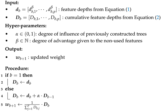
The overall procedure is completed through Algorithm 2, which implements the weighting mechanism described in Equation (4). The resulting weights are subsequently used as feature sampling probabilities for constructing the next tree. The hyperparameter $\beta$ controls the degree to which unselected features are emphasized; a larger value of $\beta$ assigns higher sampling weights to features that were not chosen in the previous trees.

Algorithm 2: Weight Updating Algorithm

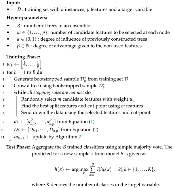
Finally, the complete procedure of the proposed Heterogeneous Random Forest (HRF) algorithm is summarized in Algorithm 3.

2.6. New Measure of Diversity

Our proposed method, HRF, seeks to improve the diversity of trees within an ensemble. In ensemble learning, diversity is often assessed using prediction-oriented measures such as the disagreement measure [18], the double-fault measure [19], or the Kohavi–Wolpert variance [20], all of which quantify how differently individual learners respond to the same input instances. While these metrics are widely used, they rely solely on the outputs of the learners and do not capture how heterogeneous the underlying tree structures are. To complement this perspective, we introduce a new tree-structure-based dissimilarity metric designed to evaluate the internal diversity encouraged by HRF. Specifically, our metric quantifies heterogeneity in terms of feature usage patterns and feature dominance across trees, offering a structural viewpoint that prediction-based metrics cannot provide. This allows us to examine whether HRF successfully induces diverse tree architectures, beyond differences observed only at the prediction level.

The structural characteristics of a decision tree can be represented by its feature depth vector, ${\mathit{d}}_b$, which specifies the depth at which each feature is used for splitting. Based on this representation, we define the concept of feature dominance, which reflects the relative importance of features within a single tree and enables quantitative comparison between different trees.

Algorithm 3: Heterogeneous Random Forest Algorithm

The dominance of the j-th feature in the b-th classifier is defined as

$$I_{b,j}=\left\{\begin{array}{c}\begin{array}{ccc}{M}_b^{*}+1-d_{b,j}^{\beta }\hfill & \hfill & \mathrm{if}{X}_j\mathrm{is}\mathrm{used}\mathrm{in}b\text{-}\mathrm{th}\mathrm{tree}\hfill \\ 0,\hfill & \hfill & \mathrm{otherwise},\hfill \end{array}\hfill \end{array}\right.$$

(5)

where $M_b^{*}$ denotes the maximum feature depth among the split variables in $h_b$. Unused features are assigned a dominance value of 0, whereas features appearing near the root node receive relatively larger values.

To compare two trees, $h_l$ and $h_m$, we concatenate their dominance vectors by row to form a $2\times p$ table, $[{\mathit{I}}_l,{\mathit{I}}_m]$. A ${\chi }^2$ test of homogeneity is then applied to this table. A large ${\chi }^2$ statistic indicates that the two trees differ substantially in their feature usage, whereas a small statistic implies structural similarity.

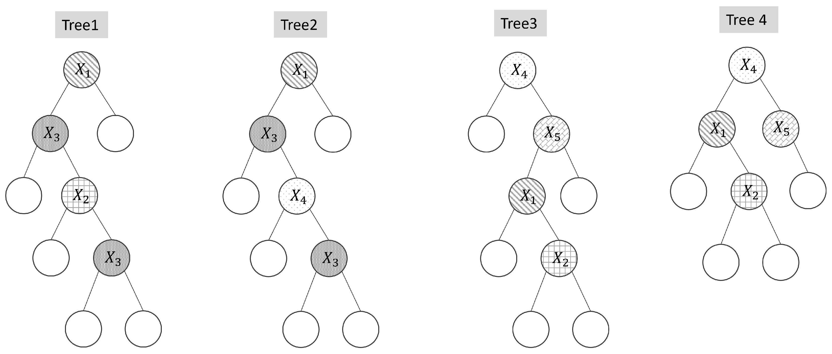
Figure 2 illustrates examples of tree dissimilarity. Trees 1 and 2, as well as Trees 3 and 4, exhibit similar structural patterns.

Table 2. Procedure to calculate dissimilarity between trees.

(a) Dominance
	$X_1$	$X_2$	$X_3$	$X_4$	$X_5$
$I_1$	3	1	2	0	0
$I_2$	3	0	2	1	0
$I_3$	2	1	0	4	3
$I_4$	1	2	0	3	2
(b) ${\chi }^2\left(\mathrm{df}\right)$ test statistics
${\chi }^2\left(\mathrm{df}\right)$	$h_1$	$h_2$	$h_3$	$h_4$
$h_1$	-	2.000(3)	8.747(4)	8.215(4)
$h_2$		-	7.467(4)	7.875(4)
$h_3$			-	0.797(4)
$h_4$				-
(c) Dissimilarity
$DS$	$h_1$	$h_2$	$h_3$	$h_4$
$h_1$	-	−0.192	1.500	1.386
$h_2$		-	1.217	1.310
$h_3$			-	−1.040
$h_4$				-

(a) presents the dominance values for each feature, while Table 2(b) reports the corresponding ${\chi }^2$ test statistics used to measure similarity between trees.

To enable comparison under varying degrees of freedom, the ${\chi }^2$ statistic can be transformed into a standard normal variable using the Wilson–Hilferty transformation [21]. The resulting dissimilarity, $DS$, between two trees, $h_l$ and $h_m$, is defined as

$$DS(h_l,h_m)={\displaystyle \frac{\sqrt[3]{X/k}-\left(1-\frac{2}{9k}\right)}{\sqrt{2/\left(9k\right)}}},$$

(6)

where X represents the ${\chi }^2$ test statistic with k degrees of freedom. Finally, Table 2(c) summarizes the resulting dissimilarity ($DS$) values. In general, larger positive dissimilarity values indicate greater structural differences between trees. As shown, the $DS$ value between Trees 1 and 2, as well as between Trees 3 and 4, is relatively small, while other tree pairs exhibit considerably higher positive values, validating the effectiveness of the proposed measure.

2.7. Scalability

The computational complexity of RF [22] is known to be $O(B·m·n·logn)$, where B is the number of trees, m is the number of candidate features considered at each split, and n is the number of training samples. HRF follows the same tree-growing process as RF, with the addition of a feature-weight update after each tree is built. This update requires only a single pass through all p features, contributing an additional $O(B·p)$ term. Therefore, the total complexity of HRF is

$$O\left(B·m·n·logn+B·p\right),$$

which differs from RF only by a lower-order linear term.

To validate this theoretical analysis, we empirically examined HRF’s training time while independently varying (i) the number of samples n, (ii) the number of features p, and (iii) the ensemble size B. All experiments were conducted on synthetic datasets in which all features were equally informative, with default settings of $n=\mathrm{10,000}$, $p=100$, and $B=100$. Each factor was varied one at a time while the others were held fixed, and the HRF-specific parameters were set to $\alpha =0.5$ and $\beta =1$. The results, summarized in Figure 3, show that HRF scales approximately linearly with n, p, and B, consistent with the theoretical complexity. These findings confirm that HRF introduces negligible computational overhead relative to RF and remains computationally feasible even for high-dimensional datasets.

3. Simulation Study

The objective of this simulation study is to examine several key aspects of the proposed HRF model. Each simulation corresponds to a binary classification task consisting of 1000 samples, of which 70% were used for training and the remaining 30% for evaluation. The ensemble comprised 100 individual trees, with the hyperparameters for tree construction set to their default values. The default values of the HRF-specific parameters $\alpha$ and $\beta$ were 0.5 and 1, respectively. To ensure robust comparison, the entire simulation procedure was repeated 100 times.

3.1. Selection Bias

We aim to assess the extent to which HRF exhibits feature selection bias, as previous studies have reported that both bagging and RF suffer from such bias due to the greedy search property of decision trees [23].

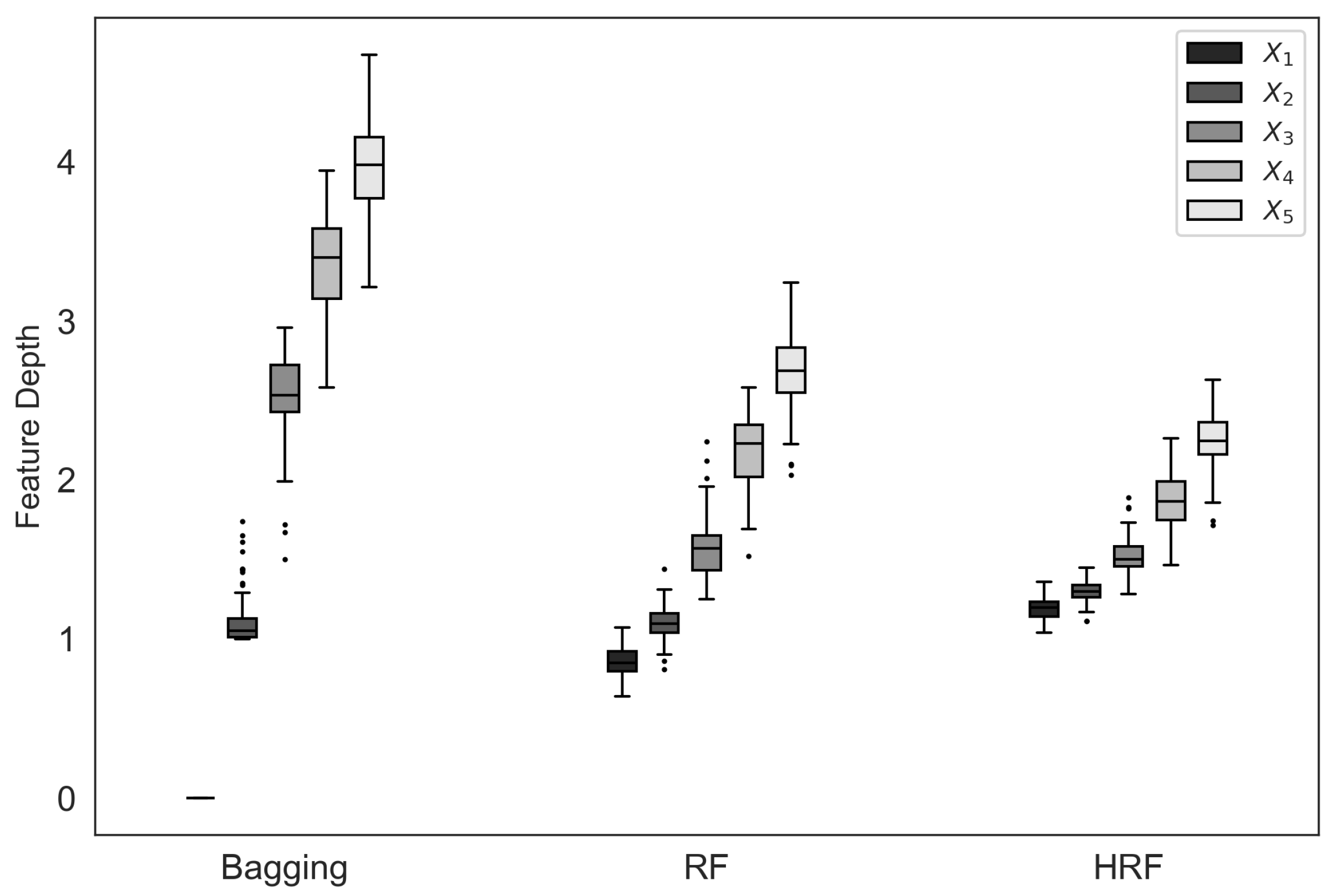
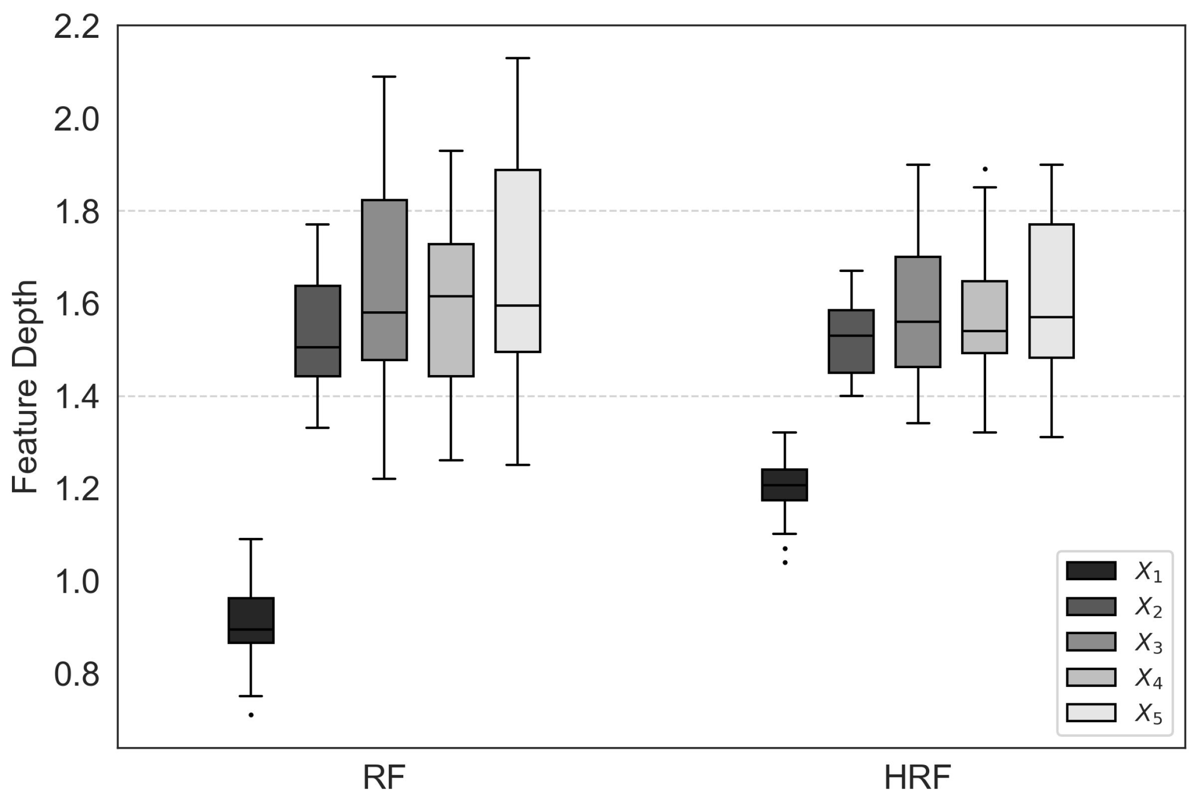
In this experiment, five input features were generated. Feature $X_1$ takes integer values between 0 and 128, $X_2$ between 0 and 64, $X_3$ between 0 and 32, $X_4$ between 0 and 16, and $X_5$ between 0 and 8, all following discrete uniform distributions. The binary target variable was generated as $\mathit{y}=\mathrm{Bernoulli}\left(\sigma (\mathit{\eta }-Q_2\left(\mathit{\eta }\right))\right)$, where $Q_2\left(\mathit{\eta }\right)$ denotes the median of $\mathit{\eta }$, $\sigma (·)$ is the sigmoid function, and $\mathrm{Bernoulli}(·)$ represents a binary random variable with the given probability. The linear predictor $\mathit{\eta }$ is defined as $\mathit{\eta }=X_1+X_2+X_3+X_4+X_5$, indicating that all five features are equally important in determining $\mathit{y}$.

The feature depth vector ${\mathit{d}}_b=[d_{b,1}^1,\dots ,d_{b,p}^1]$ represents the depth of each feature in the b-th tree within the ensemble. If selection bias exists toward features with a larger number of unique values, the feature depth of $X_1$ (i.e., $d_{b,1}^1$) will tend to be smaller, as it is more likely to be selected near the root node. Conversely, features with fewer unique values will have larger depth values. For an ensemble of 100 trees, a total of 100 feature depth values are accumulated for each feature.

Figure 4 presents box plots of feature depth values for each feature across different ensemble methods. It can be observed that both bagging and RF tend to select features with a larger number of unique values near the root nodes, a phenomenon attributable to selection bias. In particular, bagging exhibits a pronounced bias, almost always prioritizing the selection of feature $X_1$. In contrast, HRF substantially mitigates this bias, as the feature depth distributions of HRF are more balanced across features compared with Bagging and RF.

3.2. Impact on Feature Importance

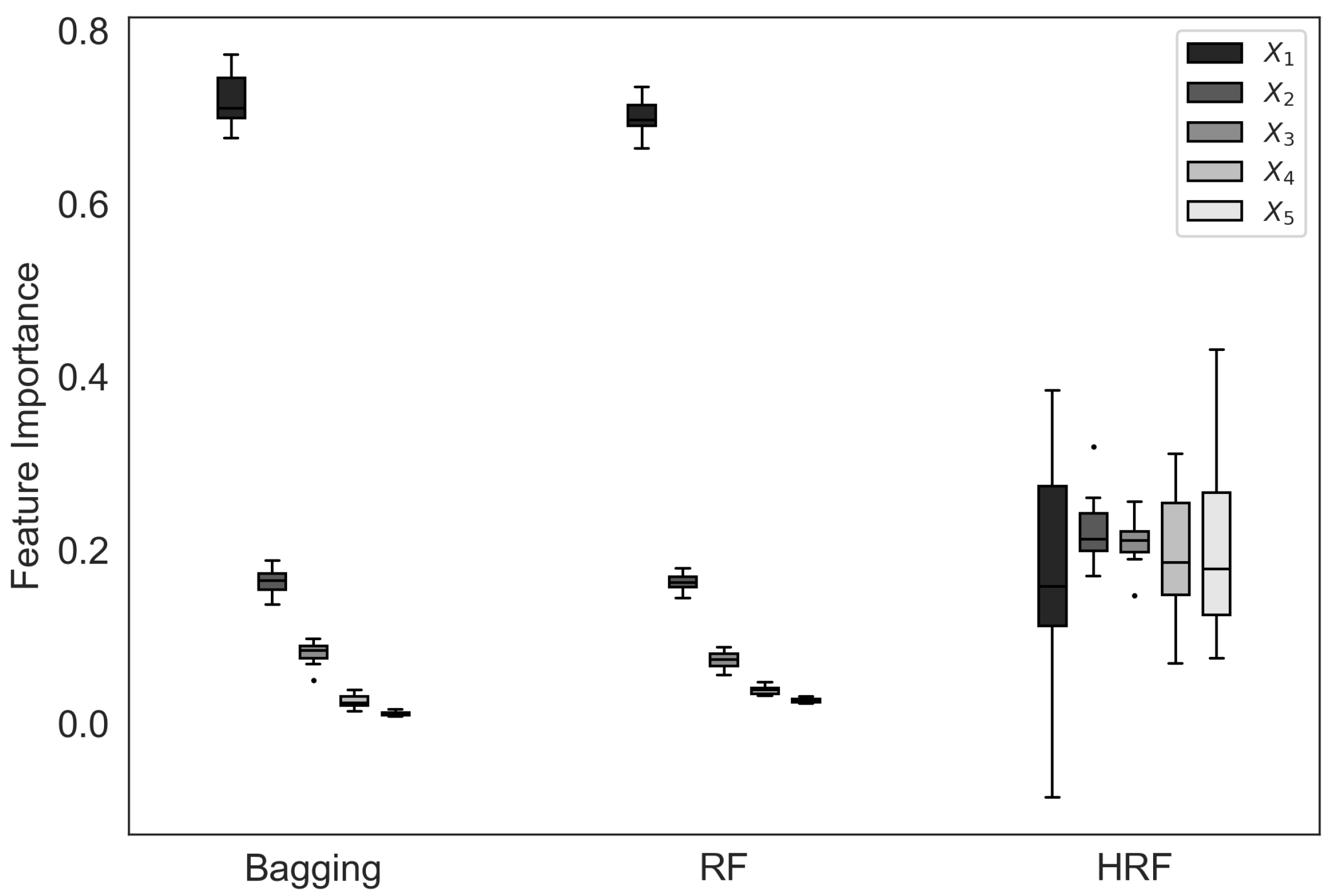
In this subsection, we investigate how feature selection bias influences the estimated feature importance of different ensemble methods. Ideally, when all input features contribute equally to the target variable, the resulting feature importance values should be similar across features. However, as shown in Figure 5, both bagging and RF display a pronounced imbalance in their importance estimates, heavily emphasizing the $X_1$ feature while underestimating the others. This indicates that the feature selection bias observed in these methods adversely affects their feature importance estimation, causing them to overvalue features with higher cardinality.

In contrast, HRF produces feature importance values that are much more evenly distributed among all five features, reflecting the true underlying structure of the data.

3.3. Dissimilarity

In this section, we examine whether HRF indeed enhances ensemble diversity relative to bagging and RF. Using the same simulation setup described in Section 3.1, we computed the tree-level dissimilarity measure $DS$ in a pairwise manner for all trees within each ensemble (see Equation (6)). The overall dissimilarity for each method was obtained by averaging all pairwise values, and the entire procedure was repeated 100 times to ensure stability of the estimates.

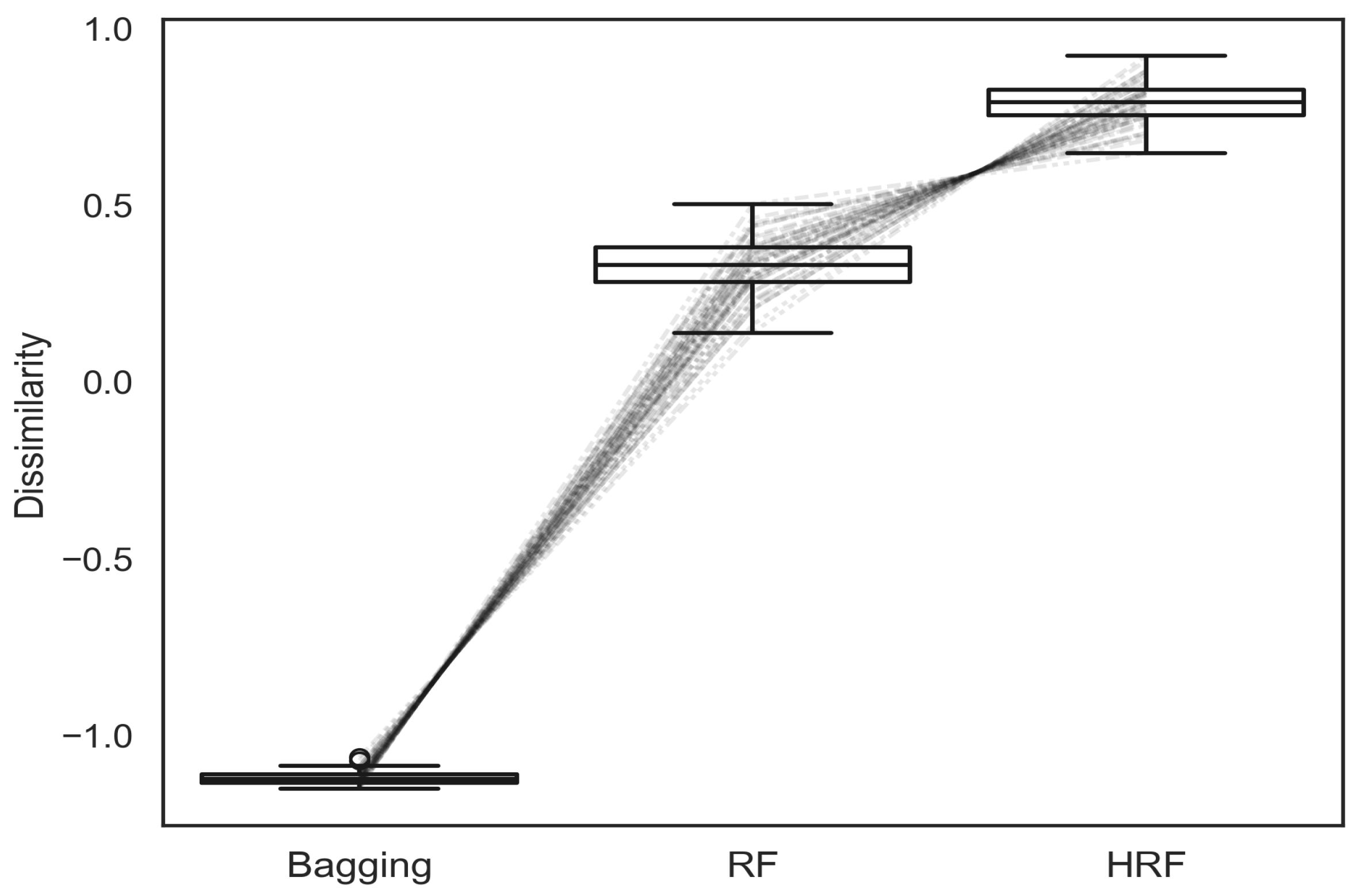
As shown in Figure 6, bagging exhibits the lowest level of structural diversity, followed by RF. HRF consistently achieves the highest dissimilarity scores among the compared methods, indicating that its asymmetric feature weighting mechanism effectively promotes more diverse tree structures.

3.4. Noise Feature Effect

As HRF assigns feature weights based on feature selection information from preceding trees, there is a potential risk of assigning higher selection weights to noise features. We intend to assess the severity of this problem.

To investigate the impact of noise features on the HRF method, a case with a total of 30 features was considered. Let $p^{*}$ denote the number of informative features. The input features $X_j,j=1,\dots ,30,$ were generated from discrete uniform distribution between 0 and 4. The target variable is generated by $\mathit{y}=bernoulli\left(\sigma (\mathit{\eta }-Q_2\left(\mathit{\eta }\right))\right)$, where $\mathit{\eta }={\sum }_{j=1}^{p^{*}}{X}_j$. In the simulation data, the noise feature ratio was increased in increments of 0.1, starting from 0 and reaching 0.7.

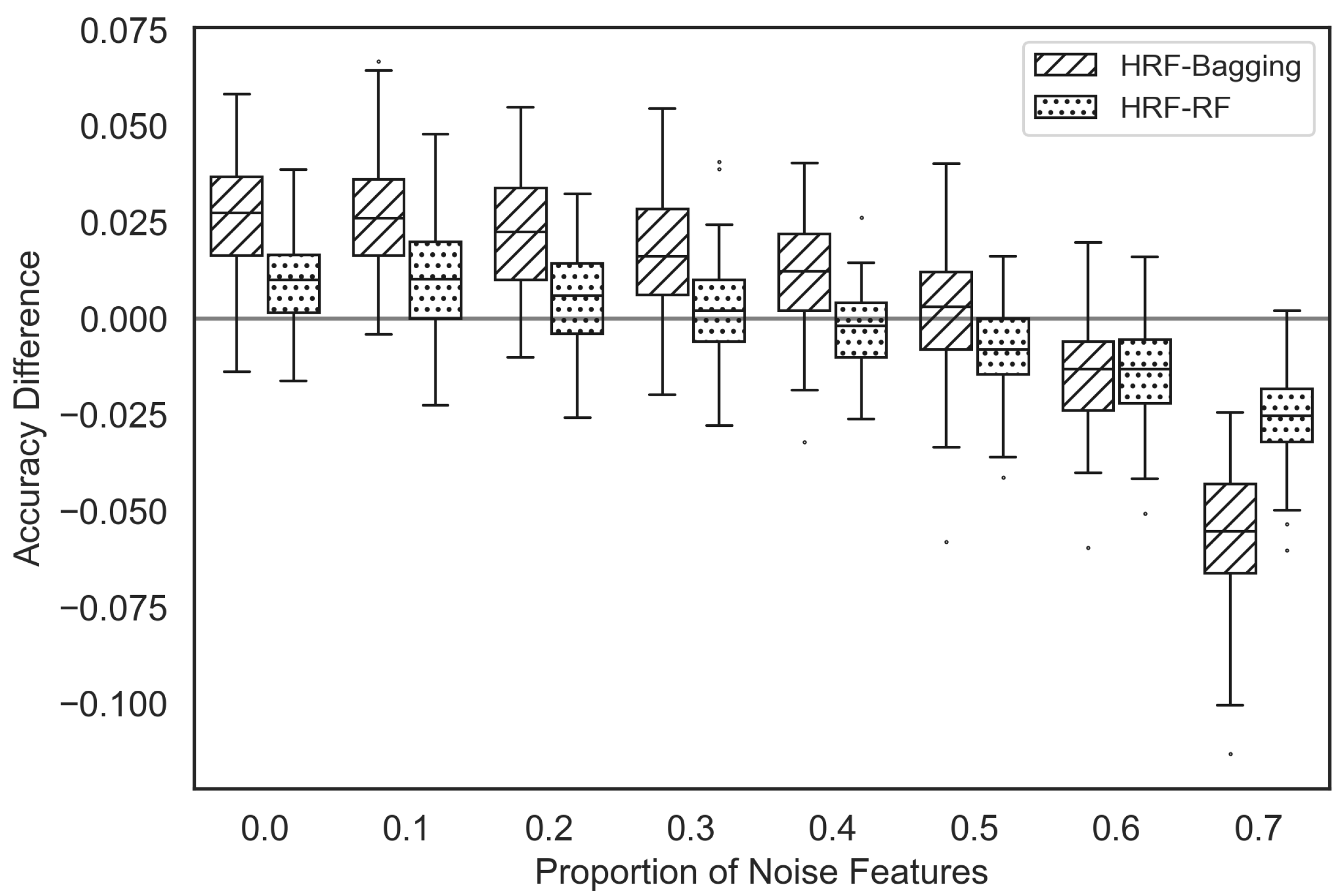
Figure 7 presents box plots showing the accuracy differences between HRF and bagging, as well as between HRF and RF. A positive value indicates that HRF exhibits higher accuracy. HRF outperforms bagging when the proportion of noise features is less than 60% of the total features. Conversely, when the proportion of noise features exceeds 60%, HRF experiences a decline in performance. Similarly, HRF outperforms RF when the proportion of noise features is below 40% of the total features; however, when the proportion exceeds 50%, HRF also sees a decrease in performance.

3.5. Hyperparameter Effect

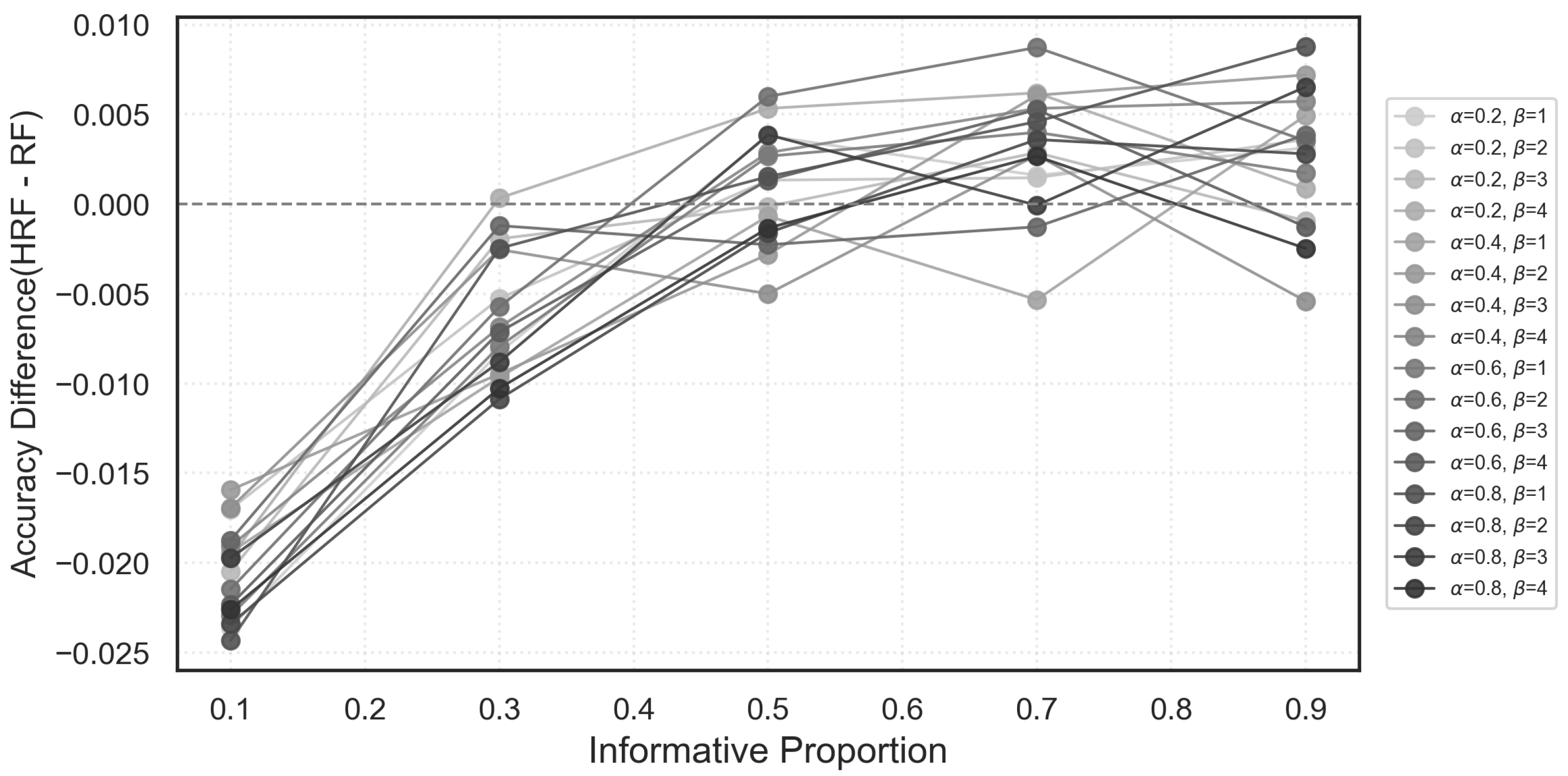
We further examined how the HRF-specific hyperparameters—the memory factor $\alpha$ and the penalty factor $\beta$—influence predictive performance. This experiment was conducted under a simulation design similar to that of Section 3.4, using datasets with 100 features and 5000 samples. Figure 8 displays the accuracy differences between HRF and RF across various combinations of $(\alpha ,\beta )$ under different proportions of informative features.

When the proportion of informative variables is moderate to high, HRF generally outperforms RF across most parameter settings, although the magnitude of improvement varies across $(\alpha ,\beta )$; this indicates that hyperparameter tuning can be beneficial in settings where many features carry meaningful signals. In contrast, when noise features dominate the feature space (i.e., informative proportion below 0.4), HRF tends to underperform RF in a consistent manner across all $(\alpha ,\beta )$ configurations. This suggests that the degradation observed in high-noise scenarios does not arise from particular hyperparameter choices but rather reflects an inherent limitation of the HRF weighting mechanism when informative variables are overwhelmed by noise.

Overall, these results indicate that while HRF exhibits mild sensitivity to $(\alpha ,\beta )$ in signal-rich environments, its performance drop in extremely noisy settings is largely independent of specific parameter values.

3.6. Effect of Correlated Features

To assess whether penalizing a dominant feature simply transfers its influence to a correlated surrogate or instead promotes exploration of non-redundant predictors, we conducted an additional simulation study. The input features $X_j(j=1,\dots ,5)$ were generated with 2000 observations, where each feature followed a standard normal distribution independently, except that a strong correlation $(\rho =0.9)$ was imposed between $X_1$ and $X_2$. The remaining features $X_3$, $X_4$, and $X_5$ were independent of $X_1$. The binary response was generated according to the linear predictor $\mathit{\eta }=2X_1+X_3+X_4+X_5$, such that only $X_1$, $X_3$, $X_4$, and $X_5$ carried true signal, while $X_2$ acted purely as a correlated surrogate.

Figure 9 compares feature-depth distributions for RF and HRF.

Under RF, the dominant feature $X_1$ consistently appears near the root, while the remaining features—including the correlated surrogate $X_2$—are typically selected much deeper in the trees. Under HRF, the depth of $X_1$ increases as expected due to penalization, but this reduction in dominance is not accompanied by a corresponding decrease in the depth of $X_2$. Instead, the non-redundant informative features $X_3$–$X_5$ tend to exhibit smaller depth values (i.e., they appear closer to the root), indicating that the additional sampling probability is distributed among distinct predictors rather than being absorbed by the correlated surrogate.

These results suggest that even in the presence of a strongly correlated pair, HRF does not merely replace one dominant feature with another; rather, it promotes a broader use of non-redundant features, contributing to increased structural diversity in the ensemble.

4. Empirical Evaluation

In order to investigate the performance of HRF, a series of experiments were conducted. The experiments were based on 52 real or artificial datasets used in previous studies or obtained from the UCI data repository [24].

Table 3. Description of data sets.

Data Set	Size	Inputs	Classes	# Missing	Source
aba *	4177	8	2		UCI (Abalone)
ail	13,750	12	2		[23]
aus *	690	14	2		UCI (Australian credit approval)
bal	625	5	3		UCI (Balance scale)
ban	1672	5	2		UCI (Bank note authentication)
bcw	683	9	2		[25]
bld	346	6	2		UCI (BUPA liver disorders)
blo	748	5	2		UCI (Blood transfusion center)
bod	507	24	2		[26]
bos *	506	13	3		UCI (Boston housing)
bre *	699	10	2	16	UCI (Wisconsin Breast Cancer)
cir	1000	10	2		R library mlbench (Circle in as square)
cmc *	1473	9	3		UCI (Contraceptive method choice)
cre *	690	15	2	67	UCI (Credit approval)
der	358	34	6		UCI (Dermatology)
dia	768	8	2		[23]
dna *	3187	60	3		R package mlbench (StatLog DNA)
eco	336	7	4		[23]
ger *	1000	20	2		UCI (German credit)
gla	214	9	6		UCI (Glass)
hea *	271	13	2		UCI (StatLog heart disease)
hil	606	100	2		UCI (Hil-valley)
imp *	205	25	6	59	UCI (Auto imports)
int	1000	10	2		[27]
ion	351	34	2		UCI (Ionosphere)
iri	150	4	3		UCI (Iris)
led	6000	7	10		UCI (LED display)
lib	359	90	15		UCI (Libra Movement)
lit	2329	69	9		[28]
mam	961	5	2	162	UCI (Mammographic mass)
mar	8777	4	10		[23]
mus	8124	22	2		UCI (Mushroom)
pid	532	7	2		UCI (PIMA Indian diabetes)
pks	195	22	2		UCI (Parkinsons)
pov	97	6	6	6	[29]
rng	1000	10	2		R library mlbench (Ringnorm)
sat	6435	36	6		UCI (StatLog satellite image)
seg	2310	19	7		UCI (Image segmentation)
smo *	2855	8	3		UCI (Attitude towards smoking restrictions)
snr	208	60	2		R library mlbench (Sonar)
spa	4601	57	2		UCI (Spambase)
spe	267	44	2		UCI (SPECETF heart)
tae *	151	5	3		KEEL (Teaching) [30]
thy	1000	10	2		UCI (Thyroid disease)
trn	1000	10	2		R library mlbench (Three norm)
twn	1000	10	2		R library mlbench (Two norm)
veh	846	18	4		UCI (StatLog vehicle silhouette)
vol *	1512	6	6	40	[23]
vot *	435	16	2		UCI (Congressional voting records)
vow	990	10	11		UCI (Vowel recognition)
wav	3600	21	3		UCI (Wave)
yea	1484	8	10		KEEL (Yeast) [30]
zoo	101	16	7		R library mlbench (zoo)

* Categorical features have been encoded.

provides a concise overview of the datasets.

We compared the proposed HRF with several representative ensemble algorithms. The candidate hyperparameters and their sources are summarized in

Table 4. Ensemble methods and their associated hyper-parameters. The default values are in bold.

Methods	Hyper-Parameter Tuning	Source
Bagging	max_features = [0.6, …, 1.0]	[33,34]
RF	max_features = [sqrt, log2, None]	[1,34]
ExtTrees	max_depth = [4, 6, None]	[12,34]
	min_samples_split = [2, 4]
Random Patches	max_features = [0.6, …, 1.0]	[13,34]
XGB	max_depth = [4, 6, 8]	[31]
	min_child_weight = [1, 2]
CatBoost	default	[32]

. Extremely Randomized Trees (ExtTrees; [12]) promote diversity by introducing stronger randomization in the tree construction process—specifically, by selecting both the split features and their thresholds completely at random. In contrast, Random Patches [13] enhance diversity by randomly sampling subsets of both training samples and features for each base learner. XGBoost [31] employs gradient boosting with regularization and shrinkage, and CatBoost [32] applies ordered target encoding and robust boosting strategies to mitigate overfitting. To evaluate classification performance, we measured the classification accuracy obtained through ensemble voting.

4.1. Experimental Setting

Any missing values were imputed using the mean for numerical features and the mode for categorical features. As an encoding method for categorical inputs, TargetEncoder [35] was employed for binary classification, while PolynomialWrapper [36] was utilized for multi-class classification to convert them into numerical ones. TargetEncoder was selected instead of one-hot encoding because it reduces dimensionality and sparsity while preserving target-dependent information that can benefit tree-based models. Likewise, PolynomialWrapper was applied to capture nonlinear feature interactions that may not be fully represented by standard tree splits.

Each dataset was randomly divided into a training set (80%) for model fitting and a test set (20%) for performance evaluation. All ensemble methods were constructed with 100 trees, and their hyperparameters were optimized through a 5-fold cross-validation process. For HRF, the same default settings as RF were used for tree construction, while the optimal values of $\alpha$ and $\beta$ were determined via 5-fold cross-validation. Specifically, $\alpha$ was varied from 0.0 to 0.9 in increments of 0.1, and $\beta$ was varied from 1 to $min(10,p)$—where p denotes the number of features—in increments of 1. To ensure statistical reliability, all experiments were repeated 50 times, and the results were evaluated using the Wilcoxon signed-rank test for pairwise statistical comparison [37].

4.2. Classification Accuracy

Table 5. Accuracy of ensemble methods: ‘+’ indicates that HRF is significantly better, while a ‘−’ indicates that HRF is significantly worse at the 0.05 significance level.

Data	Bagging	RF	ExtTrees	RndPatch	XGB	CatBoost	HRF
aba	0.7743+	0.7777+	0.7790+	0.7722+	0.7711+	0.7814	0.7818
ail	0.8805	0.8803−	0.8767+	0.8728+	0.8838−	0.8848−	0.8798
aus	0.8692+	0.8676+	0.8647+	0.8692+	0.8698+	0.8671+	0.8765
bal	0.8706	0.8467+	0.8810−	0.8652	0.8868−	0.8836−	0.8662
ban	0.9918+	0.9918+	0.9988−	0.9898+	0.9945	0.9942	0.9940
bcw	0.9717+	0.9704+	0.9714+	0.9719+	0.965+	0.971+	0.9746
bld	0.7089+	0.7175+	0.7146+	0.6994+	0.7045+	0.7159+	0.7375
blo	0.7657	0.7450+	0.7713	0.7709	0.7551+	0.7918−	0.7696
bod	0.9513+	0.9566+	0.9687−	0.9561+	0.9636	0.9711−	0.9621
bos	0.7911+	0.7921+	0.7796+	0.7899+	0.7853+	0.7887+	0.8005
bre	0.9656+	0.9670+	0.9685	0.9700	0.9581+	0.9684+	0.9701
cir	0.8263+	0.8269+	0.8291	0.8248+	0.8781−	0.8618−	0.8340
cmc	0.5191+	0.5167+	0.5227+	0.5170+	0.5372−	0.5318	0.5300
cre	0.8731+	0.8742+	0.8656+	0.8726+	0.8678+	0.8746+	0.8825
der	0.9677+	0.9744+	0.9817	0.9697+	0.9602+	0.9753+	0.9798
dia	0.7562+	0.7624+	0.7647+	0.7548+	0.7430+	0.7718	0.7706
dna	0.9621+	0.9678	0.9670	0.9654+	0.9663+	0.9656+	0.9679
eco	0.9258+	0.9368+	0.9442	0.9246+	0.9154+	0.9308+	0.9450
ger	0.7648+	0.7678+	0.7648+	0.7611+	0.7589+	0.7745	0.7728
gla	0.7438+	0.7581+	0.7403+	0.7581+	0.7319+	0.7541+	0.7688
hea	0.8195+	0.8286+	0.8323+	0.8200+	0.8079+	0.8328+	0.8407
hil	0.5674+	0.5625+	0.5536+	0.5719+	0.5744	0.5118+	0.5781
imp	0.7885	0.7810+	0.7351+	0.7911	0.7987	0.7849	0.7895
int	0.7455−	0.5946	0.5571+	0.7081−	0.8469−	0.8050−	0.5994
ion	0.9310+	0.9345	0.9394	0.9314+	0.9274+	0.9328	0.9375
iri	0.9449+	0.9493+	0.9551	0.9458+	0.9378+	0.9489+	0.9511
led	0.7340+	0.7315+	0.7334+	0.7334+	0.7323+	0.7311+	0.7354
lib	0.7748+	0.7811+	0.8141−	0.7757+	0.7119+	0.7809+	0.8006
lit	0.8808+	0.8835+	0.8815+	0.8810+	0.9055−	0.9033−	0.8878
mam	0.8295−	0.7938+	0.8227	0.8303−	0.8081+	0.8350−	0.8217
mar	0.5812	0.5400+	0.5815−	0.5814−	0.5751+	0.5678+	0.5812
pid	0.7596+	0.7706+	0.7618+	0.7613+	0.7390+	0.7772	0.7767
pks	0.8738+	0.8969+	0.8679+	0.8986+	0.9128	0.9166−	0.9055
pov	0.6090+	0.6117	0.5869+	0.6021+	0.6228	0.6386	0.6228
rng	0.9179	0.9085+	0.9374−	0.9259	0.9169	0.9231−	0.9161
sat	0.9116+	0.9139+	0.9144	0.9136+	0.9153	0.9044+	0.9151
seg	0.9777	0.9778	0.9775	0.9758+	0.9822−	0.9777	0.9783
smo	0.6986−	0.6511+	0.6983−	0.6938−	0.662+	0.6480+	0.6835
snr	0.7910+	0.8216+	0.8265+	0.8119+	0.8432	0.8416	0.8439
spa	0.9499+	0.9518+	0.9548−	0.9495+	0.9537−	0.9528	0.9527
spe	0.7990+	0.8032+	0.8040+	0.8008+	0.7953+	0.808+	0.8155
tae	0.6138+	0.6333+	0.6093+	0.6222+	0.6573−	0.6342	0.6440
thy	0.9965−	0.9963−	0.9811+	0.9928+	0.9953+	0.9960	0.9961
trn	0.8538+	0.8596+	0.8736−	0.8604+	0.8556+	0.8604+	0.8659
twn	0.9627+	0.9623+	0.9672−	0.9640	0.9587+	0.9643	0.9657
veh	0.7477+	0.7527+	0.7452+	0.7528+	0.7645	0.7645	0.7589
vol	0.8625+	0.9036	0.8893+	0.9047	0.9041	0.9073−	0.9035
vot	0.9548+	0.9548+	0.9551+	0.9511+	0.9568	0.9517+	0.9594
vow	0.9379+	0.9467+	0.9733−	0.9405+	0.8936+	0.9421+	0.9551
wav	0.8465+	0.8466+	0.8541	0.8475+	0.8474+	0.8462+	0.8516
yea	0.5933+	0.6098+	0.6062+	0.5851+	0.5808+	0.5873+	0.6201
zoo	0.9473	0.9447	0.9393+	0.9513	0.9447	0.9427	0.9507
W/T/L	(40/8/4)	(43/7/2)	(29/12/11)	(40/7/5)	(30/13/9)	(24/17/11)

W: # of dataset HRF wins, T: # of dataset tied, L: # of dataset HRF loses.

presents a comparison of the accuracy between HRF and other ensemble methods. The ‘+’ symbol indicates that HRF showed statistically more accurate results than the corresponding method, whereas the ‘−’ symbol indicates less accurate results. The ‘W/T/L’ at the bottom row represents the number of datasets where HRF was better/equal/worse compared to the respective method.

Table 6. Summary of comparisons among methods.

	Bagging	RF	ExtTree	RndPatch	XGB	CatBoost	HRF
Bagging		35(22)	33(25)	31(12)	24(19)	37(30)	45(40)
RF	17(8)		30(19)	22(11)	29(23)	32(22)	48(43)
ExtTree	20(12)	22(14)		17(14)	22(15)	30(21)	35(29)
RndPatch	22(8)	31(18)	35(26)		23(18)	37(27)	43(40)
XGB	28(22)	24(21)	30(24)	29(18)		31(26)	35(30)
CatBoost	15(7)	20(8)	22(19)	15(6)	22(11)		33(24)
HRF	7(4)	4(2)	17(11)	9(5)	18(9)	19(11)

In each cell, the results are summarized as ‘$a\left(b\right)$’, where a indicates the number of datasets where the method in the column outperforms the method in the row, and b indicates the number of datasets where this difference is statistically significant according to the one-sided paired t-test.

displays pairwise comparisons among the methods. The values in the table show the number of instances where the method listed vertically is more accurate than the method listed horizontally, with the number in parentheses denoting statistical significance. To illustrate, a value of 35(22) in the first row and second column indicates that RF outperforms the Bagging method in 35 out of 52 datasets, with 22 of those instances being statistically significant. In cases where the accuracy values are the same, a value of 0.5 was assigned.

Table 7. The dominance rank of the methods determined by the significant difference from the results in Table 6.

Methods	Wins	Losses	Dominance Rank
HRF	206	42	164
CatBoost	137	75	62
ExtTree	124	105	19
RF	85	126	−41
XGB	95	141	−46
RndPatch	66	137	−71
Bagging	61	148	−87

summarises the ranking of methods according to the results presented in Table 6. The dominance rank is calculated as the difference between the number of significant wins and significant losses. For example, HRF achieves a dominance rank of 164, derived from a total of 206 significant wins and 42 significant losses. The number of significant wins for HRF is equal to the cumulative sum of the values within parentheses in the HRF columns of Table 6. Similarly, the number of significant losses for HRF is the sum of the values within parentheses in the HRF row. Table 6 and Table 7 collectively demonstrate that the HRF method exhibits significant superiority over other methods across a dataset pool comprising 52 instances.

4.3. Noise Feature Effect

In Section 3.4, we investigated the effects of noise features on HRF. Specifically, when the number of noise features is excessively large, HRF tends to perform worse than bagging and RF. In this section, we further examined whether a similar pattern is observed in experiments with real datasets.

To estimate the proportion of noise features in each dataset, a deep decision tree was trained to compute feature importance values for all variables. Let the feature importance vector be denoted as $\mathit{I}=[I_1,\dots ,I_p]$, which was normalized as $\mathit{I}\leftarrow [I_1,\dots ,I_p]/{\sum }_j{I}_j$. If the scaled feature importance was smaller than $1/p$, that is, $I_j<{\displaystyle \frac{1}{p}}$, the corresponding feature was regarded as noise. The resulting proportion of noise features (p_noise$={\displaystyle \frac{\#\mathrm{noise}\mathrm{features}}{p}}$) is summarized in

Table 8. The estimated proportions of noise features.

Data Set	p_noise	Data Set	p_noise	Data Set	p_noise
aba	0.63	ger	0.65	sat	0.92
ail	0.75	gla	0.44	seg	0.79
aus	0.79	hea	0.69	smo	0.7
bal	0.25	hil	0.6	snr	0.75
ban	0.75	imp	0.78	spa	0.79
bcw	0.89	int	0.8	spe	0.7
bld	0.67	ion	0.85	tae	0.71
blo	0.5	iri	0.75	thy	0.81
bod	0.79	led	0.43	trn	0.4
bos	0.71	lib	0.68	twn	0.6
bre	0.89	lit	0.77	veh	0.67
cir	0.7	mam	0.6	vol	0.71
cmc	0.85	mar	0.75	vot	0.94
cre	0.73	pid	0.57	vow	0.7
der	0.82	pks	0.73	wav	0.71
dia	0.75	pov	0.67	yea	0.5
dna	0.9	rng	0.5	zoo	0.69
eco	0.71

.

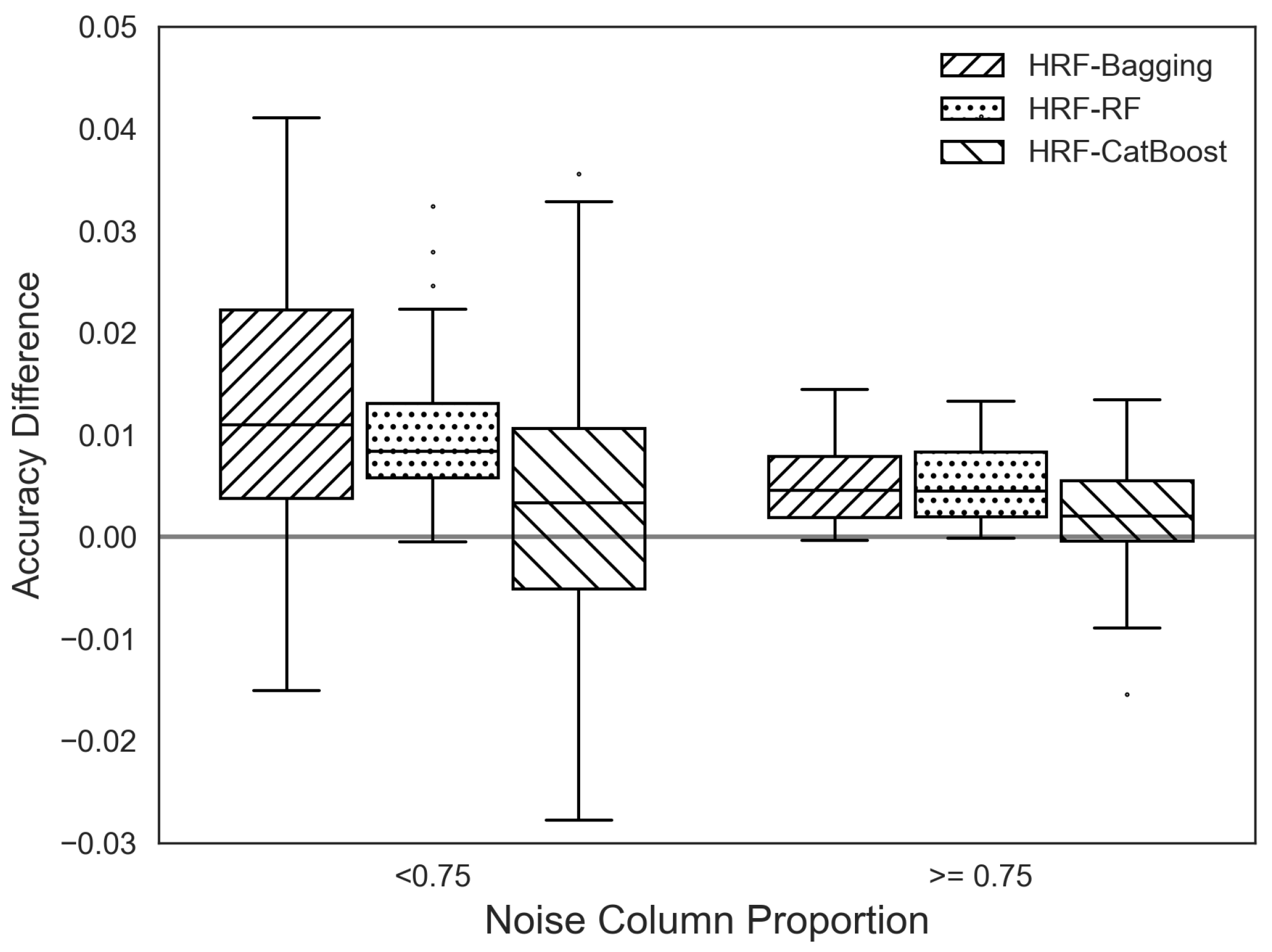
We divided all datasets into two groups based on a noise ratio threshold of 0.75. Then, using the accuracy differences between HRF and other ensemble methods within each group, we generated box plots, as shown in Figure 10. The results indicate that HRF achieves relatively higher accuracy improvements over bagging and RF in datasets with lower proportions of noise features, consistent with the earlier simulation findings.

Unlike bagging and RF, the accuracy difference between HRF and CatBoost does not show a clear dependence on the proportion of noise features. This observation suggests that the difference in accuracy is primarily attributable to fundamental distinctions in model structure and learning mechanisms: CatBoost employs gradient boosting with ordered target encoding and regularization, whereas HRF enhances diversity through adaptive feature weighting within a bagging framework.

4.4. Hyperparameter Selection

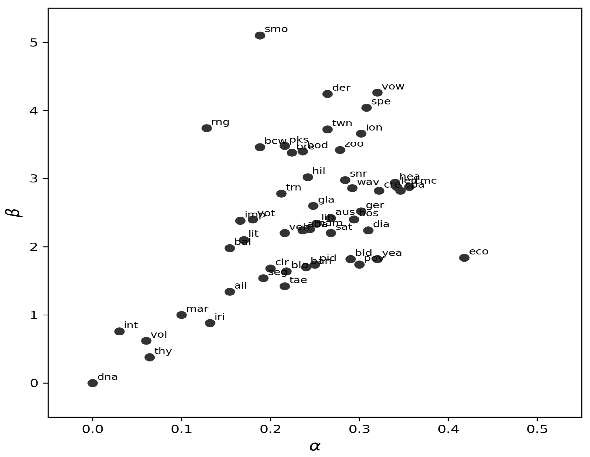
We analyzed the stability and distribution of the optimal values selected through cross-validation across the 52 benchmark datasets. Specifically, for each dataset, the $(\alpha ,\beta )$ pair was chosen via 5-fold cross-validation, repeated 50 times under identical train–test splits to ensure robustness.

Figure 11 summarizes the empirical distribution of the selected $(\alpha ,\beta )$ values across all datasets. Despite variability across data domains, a clear concentration pattern emerges: most optimal values lie within the ranges $\alpha \in [0.1,0.4]$ and $\beta \in [1,4].$ This clustering indicates that simple near-default configurations (e.g., $\alpha =0.3$, $\beta =2.5$) can often provide competitive performance, reducing the practical burden of extensive hyperparameter tuning.

4.5. Discussion

The empirical evaluation demonstrates that the proposed Heterogeneous Random Forest (HRF) consistently achieves competitive or superior classification accuracy compared with conventional ensemble methods across 52 benchmark datasets. As summarized in Table 7, HRF achieved the highest dominance rank among all compared methods, indicating its superiority in predictive performance across diverse datasets. The improvements observed in HRF can be attributed to its adaptive and asymmetric feature weighting mechanism, which promotes feature diversity and mitigates the repetitive selection of dominant features. This mechanism enables HRF to better balance the utilization of informative features, leading to enhanced generalization performance without introducing additional model complexity.

The analysis of noise-feature effects further compared HRF and RF to examine how performance changes under varying levels of irrelevant or noisy variables. The results revealed that HRF shows its greatest advantage in datasets with relatively low proportions of noise features. As the proportion of irrelevant or noisy variables increases, HRF’s benefit tends to diminish, and in some cases, its accuracy becomes comparable to that of RF. This outcome is consistent with HRF’s design philosophy—its adaptive weighting is most effective when meaningful features are present and not overwhelmed by noise. When the same analysis was extended to CatBoost, the accuracy difference between HRF and CatBoost did not show a clear dependence on the proportion of noise features. This suggests that, unlike bagging-based ensembles where diversity plays a central role, CatBoost’s performance is primarily governed by its gradient-based optimization and regularization mechanisms.

Overall, these findings indicate that HRF is particularly effective in improving predictive performance when datasets contain a balanced and informative set of features. However, its relative advantage may be reduced in high-noise environments, suggesting that pre-filtering of irrelevant variables or feature selection techniques could further enhance its robustness in practical applications.

5. Conclusions

In this study, we proposed the Heterogeneous Random Forest (HRF), an ensemble method that extends the Random Forest (RF) framework through adaptive and asymmetric feature weighting designed to promote structural diversity among decision trees. HRF introduces several methodological mechanisms that contribute to improved ensemble performance:

• Asymmetric Feature Weighting: Sampling probabilities are adaptively updated based on feature usage history, reducing the tendency to repeatedly select dominant features.
• Mitigation of Feature Selection Bias: HRF alleviates RF’s well-known preference for high-cardinality variables, enabling more balanced utilization of informative low-cardinality features.
• Enhanced Ensemble Diversity: By discouraging redundant split patterns, HRF yields more heterogeneous tree structures, which in turn improve generalization performance.

Together, these mechanisms reduce repeated reliance on dominant features and encourage exploration of underutilized but potentially meaningful variables, resulting in more balanced feature usage and improved predictive accuracy without increasing model complexity. Simulation studies and empirical analyses further demonstrated that HRF performs particularly well when the dataset contains meaningful signals and diverse feature characteristics. Although its relative advantage diminishes when irrelevant or noisy features dominate, HRF still maintains performance comparable to RF, indicating strong overall stability.

Across 52 benchmark datasets, HRF achieved the highest dominance rank among all compared ensemble algorithms, outperforming Bagging, RF, Extremely Randomized Trees, Random Patches, and boosting-based models such as XGBoost and CatBoost. HRF showed significant improvements over RF in 43 out of 52 datasets, confirming its robustness and consistent predictive advantage in practice.

We also introduced a new structural dissimilarity metric based on feature dominance and the ${\chi }^2$ test to quantify internal diversity within ensembles. This measure revealed that HRF produces more heterogeneous decision trees than conventional ensemble methods, providing empirical evidence that encouraging structural diversity at the feature-selection level can translate into measurable performance gains.

Overall, HRF offers a practical and theoretically grounded enhancement to traditional ensemble learning by improving feature-level diversity and mitigating selection bias. It represents a promising approach for classification tasks that require robust, diverse ensemble models across a broad range of data domains.

• Future Work. There remain several directions for extending this work. First, exploring strategies to improve HRF’s robustness in high-noise environments would be valuable. Initial feature filtering—using statistical tests or preliminary feature-importance screening—may help reduce the influence of irrelevant variables, while less aggressive adjustments to the adaptive weight update rule could improve stability.

Second, a comprehensive comparison between the proposed structural dissimilarity measure $DS$ and established prediction-oriented diversity indices (e.g., disagreement, double-fault, and Kohavi–Wolpert variance) would clarify the relationships among different diversity notions and further validate $DS$ as a structural proxy for ensemble diversity.

These directions provide a basis for future methodological development and for adapting HRF to real-world applications where noise levels and feature characteristics are highly variable.

References

- Breiman, L. Random Forests. Mach. Learn. 2001, 45, 5–32. [Google Scholar] [CrossRef] [PubMed]
- Nanni, L.; Lumini, A. Input Decimated Ensemble based on Neighborhood Preserving Embedding for spectrogram classification. Expert Syst. Appl. 2009, 36, 11257–11261. [Google Scholar] [CrossRef]
- Kumar, A.; Yadav, J. A review of feature set partitioning methods for multi-view ensemble learning. Inf. Fusion 2023, 100, 101959. [Google Scholar] [CrossRef]
- Campos, Y.; Estrada, R.; Morell, C.; Ferri, F.J. A Feature Set Decomposition Method for the Construction of Multi-classifier Systems Trained with High-Dimensional Data. In Progress in Pattern Recognition, Image Analysis, Computer Vision, and Applications; Ruiz-Shulcloper, J., Sanniti di Baja, G., Eds.; Springer: Berlin/Heidelberg, Germany, 2013; pp. 278–285. [Google Scholar]
- Rokach, L. Using recursive feature elimination in random forest to account for correlated variables in high dimensional data. BMC Genet. 2008, 19, 65. [Google Scholar] [CrossRef]
- Conn, D.; Ngun, T.; Li, G.; Ramirez, C. Fuzzy Forests: Extending Random Forest Feature Selection for Correlated, High-Dimensional Data. J. Stat. Softw. 2019, 91, 1–25. [Google Scholar] [CrossRef]
- Rokach, L. Genetic algorithm-based feature set partitioning for classification problems. Pattern Recognit. 2008, 41, 1676–1700. [Google Scholar] [CrossRef]
- Rodriguez, J.; Kuncheva, L.; Alonso, C. Rotation Forest: A New Classifier Ensemble Method. IEEE Trans. Pattern Anal. Mach. Intell. 2006, 28, 1619–1630. [Google Scholar] [CrossRef]
- Chen, Y.C.; Ha, H.; Kim, H.; Ahn, H. Canonical Forest. Comput. Stat. 2014, 29, 849–867. [Google Scholar] [CrossRef]
- Rainforth, T.; Wood, F. Canonical Correlation Forests. arXiv 2015, arXiv:1507.05444. [Google Scholar] [CrossRef]
- Han, S.; Kim, H.; Lee, Y.S. Double random forest. Mach. Learn. 2020, 109, 1569–1586. [Google Scholar] [CrossRef]
- Geurts, P.; Ernst, D.; Wehenkel, L. Extremely randomized trees. Mach. Learn. 2006, 63, 3–42. [Google Scholar] [CrossRef]
- Louppe, G.; Geurts, P. Ensembles on Random Patches. In Machine Learning and Knowledge Discovery in Databases; Flach, P.A., De Bie, T., Cristianini, N., Eds.; Springer: Berlin/Heidelberg, Germany, 2012; pp. 346–361. [Google Scholar]
- Xu, B. Classifying Very High-Dimensional Data with Random Forests Built from Small Subspaces. Int. J. Data Warehous. Min. 2012, 8, 44–63. [Google Scholar] [CrossRef]
- Cabrera, J.; Lee, Y.S.; Dhammika, A. Enriched random forests. Bioinformatics 2008, 24, 2010–2014. [Google Scholar] [CrossRef] [PubMed]
- Li, X.; Ng, M.K.; Huang, J.Z.; Wu, Q.; Ye, Y. Stratified sampling for feature subspace selection in random forests for high dimensional data. Pattern Recognit. 2013, 46, 769–787. [Google Scholar] [CrossRef]
- Nguyen, T.T.; Huang, J.Z.; Nguyen, T.T.; Wang, Q. An efficient random forests algorithm for high dimensional data classification. Adv. Data Anal. Classif. 2018, 12, 953–972. [Google Scholar] [CrossRef]
- Giacinto, G.; Roli, F. Design of effective multiple classifier systems by clustering of classifiers. Pattern Recognit. Lett. 2001, 24, 1959–1969. [Google Scholar]
- Kuncheva, L.I.; Whitaker, C.J. Measures of Diversity in Classifier Ensembles and Their Relationship with the Ensemble Accuracy. Mach. Learn. 2003, 51, 181–207. [Google Scholar] [CrossRef]
- Kohavi, R.; Wolpert, D.H. Bias plus variance decomposition for zero-one loss functions. In Proceedings of the 13th International Conference on Machine Learning, Bari, Italy, 3–6 July 1996; Morgan Kaufmann: Cambridge, MA, USA, 1996; pp. 275–283. [Google Scholar]
- Wilson, E.B.; Hilferty, M.M. The Distribution of Chi-Square. Proc. Natl. Acad. Sci. USA 1931, 17, 684–688. [Google Scholar] [CrossRef]
- Probst, P.; Wright, M.N.; Boulesteix, A.L. Hyperparameters and tuning strategies for random forest. WIREs Data Min. Knowl. Discov. 2019, 9, e1301. [Google Scholar] [CrossRef]
- Loh, W.Y. Improving the precision of classification trees. Ann. Appl. Stat. 2009, 3, 1710–1737. [Google Scholar] [CrossRef]
- Dua, D.; Graff, C. UCI Machine Learning Repository. University of California, Irvine, School of Information and Computer Sciences. 2019. Available online: http://archive.ics.uci.edu/ml (accessed on 1 January 2024).
- Lim, T.S.; Loh, W.Y.; Shih, Y.S. A comparison of prediction accuracy, complexity, and training time of thirty-three old and new classification algorithms. Mach. Learn. 2000, 40, 203–228. [Google Scholar] [CrossRef]
- Heinz, G.; Peterson, L.J.; Johnson, R.W.; Kerk, C.J. Exploring Relationships in Body Dimensions. J. Stat. Educ. 2003, 11. Available online: https://jse.amstat.org/v11n2/datasets.heinz.html (accessed on 9 December 2025). [CrossRef]
- Kim, H.; Kim, H.; Moon, H.; Ahn, H. A weight-adjusted voting algorithm for ensembles of classifiers. J. Korean Stat. Soc. 2011, 40, 437–449. [Google Scholar] [CrossRef]
- Peng, R.D.; Hengartner, N.W. Quantitative Analysis of Literary Styles. Am. Stat. 2002, 56, 175–185. [Google Scholar] [CrossRef]
- Kim, H.; Loh, W.Y. Classification Trees With Unbiased Multiway Splits. J. Am. Stat. Assoc. 2001, 96, 589–604. [Google Scholar] [CrossRef]
- Alcalá-Fdez, J.; Fernandez, A.; J. Luengo, J.D.; García, S.; Sánchez, L.; Herrera, F. KEEL Data-Mining Software Tool: Data Set Repository, Integration of Algorithms and Experimental Analysis Framework. J. -Mult.-Valued Log. Soft Comput. 2011, 17, 255–287. [Google Scholar]
- Chen, T.; Guestrin, C. XGBoost: A scalable tree boosting system. In Proceedings of the 22nd ACM SIGKDD International Conference on Knowledge Discovery and Data Mining, San Francisco, CA, USA, 13–17 August 2016; ACM Press: San Francisco, CA, USA, 2016; pp. 785–794. [Google Scholar] [CrossRef]
- Dorogush, A.V.; Gulin, A.; Gusev, G.; Kazeev, N.; Prokhorenkova, L.O.; Vorobev, A. Fighting biases with dynamic boosting. arXiv 2017, arXiv:1706.09516. [Google Scholar]
- Breiman, L. Bagging predictors. Mach. Learn. 1996, 24, 2010–2014. [Google Scholar] [CrossRef]
- Pedregosa, F.; Varoquaux, G.; Gramfort, A.; Michel, V.; Thirion, B.; Grisel, O.; Blondel, M.; Prettenhofer, P.; Weiss, R.; Dubourg, V.; et al. Scikit-learn: Machine Learning in Python. J. Mach. Learn. Res. 2011, 12, 2825–2830. [Google Scholar]
- McGinnis, W.D.; Siu, C.; S, A.; Huang, H. Category Encoders: A scikit-learn-contrib package of transformers for encoding categorical data. J. Open Source Softw. 2018, 3, 501. [Google Scholar] [CrossRef]
- Raschka, S. MLxtend: Providing machine learning and data science utilities and extensions to Python’s scientific computing stack. J. Open Source Softw. 2018, 3, 638. [Google Scholar] [CrossRef]
- Rey, D.; Neuhäuser, M. Wilcoxon-Signed-Rank Test. In International Encyclopedia of Statistical Science; Springer: Berlin/Heidelberg, Germany, 2011; pp. 1658–1659. [Google Scholar] [CrossRef]
Figure 1.
Decision tree examples. The feature inside the node is the split variable and the features in brackets next to the node represent candidate features.
Figure 2.
Illustrative examples of decision trees used for dissimilarity evaluation. Each variable is indicated with a different shading pattern.
Figure 3.
Empirical scalability of HRF with respect to sample size, feature size, and ensemble size.
Figure 4.
Box plot of feature depths.
Figure 5.
Feature importances by method.
Figure 6.
Dissimilarity of trees by ensemble methods. Each line represents the result of 100 repeated experiments.
Figure 7.
Accuracy differences between HRF and bagging, and between HRF and RF, based on the proportion of noise features. A positive value indicates that the HRF model exhibits superior accuracy.
Figure 8.
Accuracy differences between HRF and RF across various combinations and proportions of informative features.
Figure 9.
Feature-depth distributions under RF and HRF in the presence of a highly correlated surrogate ( between and ).
Figure 10.
Box plots for the accuracy difference between HRF and others.
Figure 11.
A scatter plot of the optimal values for each of the 52 benchmark datasets, with the dataset names shown next to the points.