Symmetry-Aware Face Illumination Enhancement via Pixel-Adaptive Curve Mapping

Abstract

Face recognition under uneven illumination conditions presents significant challenges, as asymmetric shadows often obscure facial features while overexposed regions lose critical texture details. To address this problem, a novel symmetry-aware illumination enhancement method named face shadow detection network (FSDN) is proposed, which features a nested U-Net architecture combined with Gaussian convolution. This method enables precise illumination intensity maps for the given face images through higher-order quadratic enhancement curves, effectively extending the low-light dynamic range while preserving essential facial symmetry. Comprehensive evaluations on the Extended Yale B and CMU-PIE datasets demonstrate the superiority of the proposed FSDN over conventional approaches, achieving structural similarity (SSIM) indices of 0.48 and 0.59, respectively, along with remarkably low face recognition error rates of 1.3% and 0.2%, respectively. The key innovation of this work lies in its simultaneous optimization of illumination uniformity and facial symmetry preservation, thereby significantly improving face analysis reliability under challenging lighting conditions.

1. Introduction

Face recognition has achieved remarkable progress with widespread applications in human–computer interaction, criminal investigation, and multimedia systems, yet it remains significantly challenged by uneven and extreme illumination conditions. Notably, facial images possess inherent symmetrical characteristics that make them particularly vulnerable to illumination variations, as asymmetric lighting can distort these fundamental symmetric properties. Some studies point out that compared with individual difference, uneven illumination causes more changes in face image texture [1,2]. Moreover, some experts believe that illumination affects the results of face recognition more than posture [3]. These studies highlight the urgent need for effective lighting pretreatment, with the main challenge being to achieve uniform illumination. This process requires correcting asymmetrical lighting components while preserving the natural structural symmetry of the face. Therefore, to address the issues caused by uneven lighting, illuminance enhancement is often regarded as a preprocessing step for the practical application of face images.

Numerous strategies have been devised to address the challenge of illumination variation in face recognition. The classic methods include the ones using histogram equalization (HE) [4,5,6,7,8,9] and quotient image (QI) [10,11,12]. Nevertheless, they usually lack distinctiveness and cannot adapt to complex facial changes. For instance, HE does not work in those images with distinctively different background and foreground, and the Retinex-based illumination invariant feature extraction method often produces a halo phenomenon after processing the image. Most recently, experts have completed illumination enhancement by training a deep learning model to map low-light images to normal images [13,14,15,16,17,18]. However, directly mapping multiple images with different illuminations to a pair of images with normal illumination often prevents the network from fitting or finding the correct convergence point. If the fitting is forced, the structure of the processed image would be distorted. Different from the illumination enhancement of other types of images, face images are highly sensitive to structural distortions, and even slight facial structural distortions could cause difficulties in recognition. In recent years, many innovative approaches have emerged in the field of low-light image enhancement. Xie et al. [19] proposed residual quotient learning, which adaptively adjusted pixel brightness through quotient mapping but lacked global illumination modeling. Yang et al. [20] developed Zero-TCE that integrated three high-order curves in HSV space for multidimensional enhancement, though with increased complexity. Feng et al. [21] introduced HVI-CIDNet, achieving decoupled color–brightness enhancement in a novel HVI color space with superior flexibility but higher computational demands. These methods each offer unique advantages with different effectiveness–efficiency trade-offs.

To address these challenges, an innovative pixel-wise facial illumination enhancement solution is given via the proposed illumination intensity measurement algorithm. It includes two key modules: illumination intensity measurement module and illumination enhancement module. The illumination intensity measurement module is used to generate the illumination intensity map, which consists of a novel face shadow detection network (FSDN) and Gaussian convolution. The illumination enhancement module maps the low-light pixels in an image to a wider dynamic range. This is achieved by the high-order curve which is controlled by the illumination intensity map. At the same time, the proposed method can generate a reasonable and smooth transition light intensity map, which can then be used as the exposure control parameter to drive the higher-order secondary enhancement curve so as to achieve targeted enhancement of low-light areas and fine preservation of textures in normal lighting areas. Two datasets, CMU-PIE and Extended Yale B, storing face images with different illumination modes, were selected for the experiments [22,23]. As shown in the visual results, the proposed scheme effectively enhances the low-light area and retains the personalized identity features in the face images. The processed images are also analyzed, including their image quality and face recognition rate. The results show that the solution in this work is more advantageous than others.

This work has contributed in the following ways:

(1)

A symmetry-aware illumination intensity measurement algorithm is created, which combines a novel nested U-Net structure for face shadow detection with Gaussian convolution.

(2)

A high-order enhancement curve controlled by the illumination intensity is proposed, which not only maps pixels to a wider dynamic range, but also maintains the balanced enhancement of symmetrical facial features.

The remaining content is arranged as follows. Section 2 discusses related work, with a focus on illumination enhancement techniques. Section 3 describes the proposed face illumination measurement algorithm and the enhancement curve. Section 4 presents the experimental methodology, including an evaluation of the FSDN and a comprehensive analysis of the illumination enhancement results. Finally, Section 5 concludes with the limitations of the study and suggests directions for future research.

2. Related Work

This section reviews existing illumination enhancement approaches, analyzing their respective methodologies and performance characteristics. As shadow detection constitutes a core component of the proposed method, related works in this field are systematically reviewed.

2.1. Low-Light Image Enhancement

At present, there are various illumination normalization methods. HE is one of the classic conventional solutions which achieves illumination enhancement through expanding the dynamic range of images [4]. However, this method struggles with images with significant differences between the foreground and background. To address this challenge, experts have developed several variants of enhanced HE with unique technical characteristics: Block-based HE (BHE) [5] divides the image into sub-regions for local contrast enhancement but often produces blocking artifacts at patch boundaries. Adaptive histogram equalization (AHE) [8] uses sliding window processing with dynamic range clipping to suppress noise amplification, but the computational cost is increased. Oriented local histogram equalization (OLHE) [9] introduces directional kernels to preserve edge structures, achieving better structural similarity (SSIM) than BHE. In contrast, local normalization techniques (LNTs) uniquely maintain illuminated invariant local statistics through score normalization, which is faster than AHE while avoiding over-enhancement artifacts common in HE-based methods. Xie et al. [6] proposed a method that combines LNT and HE to address the issue of uneven illumination, thereby improving the performance of face detection. The other classic method is based on QI [19]. For instance, prior work proposed a nine-dimensional facial illumination subspace using QI, constructed a lower-dimensional training matrix, and achieved face illumination normalization [10]. Another solution based on QI is to normalize illumination by changing different scales features of the facial images. Motivated by the assumption that illumination influences low-frequency components, researchers proposed the NPL-QI [11] and NPLE-QI [12] methods.

In recent years, deep learning has been extensively employed in image visual tasks, including denoising, super-resolution, illumination enhancement, etc. Data-driven illumination enhancement methods can be broadly categorized into two groups, with one based on an end-to-end learning framework and the other based on an unsupervised learning framework. The end-to-end method usually achieves illumination enhancement by establishing and training the mapping relationship between abnormal illumination images and normal illumination images. Low-light net (LLNet) [13] is one of the earliest end-to-end enhancement solutions. In this framework, synthetic low-light training data was generated through gamma correction and Gaussian noise injection. Experimental results demonstrated that a stacked sparse denoising autoencoder trained on such synthetic data effectively enhances low-light images. Then, using synthetic data, LLNet is trained by the generated data and tested by the real low-light images to demonstrate the effectiveness of the training model. Shen et al. [14] argued that the traditional multi-scale Retinex (MSR) algorithm could be considered a feedforward convolution neural network with different Gaussian convolution kernels, and established MSR-net based on convolutional neural networks (CNN). In their methods, high-quality images adjusted by Photoshop and corresponding synthetic low-light images were used for training data. Inspired by the Retinex model, some deep networks estimated the reflectance and illumination of an input image by supervised learning with paired data. On the 2000-image test set, the proposed method achieves state-of-the-art performance with an SSIM score of 0.94 (the highest among compared methods) and an average NIQE value of 2.54 (the lowest recorded), demonstrating statistically significant improvements over existing approaches. Wei et al. [15] introduced the Retinex-Net which consisted of Decom-Net and Enhance-Net. The Decom-Net can split the image and obtain the illumination and reflectance. The Enhance-Net enhances the resulting illumination, which is multiplied by the original reflectance to obtain the enhanced result. Zhang et al. [16] subsequently introduced the KinD framework, which integrated three core components: Decomposition-Net, Restoration-Net, and Adjustment-Net. For the Decomposition-Net, two new loss functions are added to put a cap on the regional smoothness and consistency of the illumination graph compared with Retinex-Net. For the Restoration-Net, reflection maps under adequate lighting are used as a reference considering the degradation effect of reflection maps under low illumination. The Adjustment-Net provides a mapping function to flexibly adjust light levels based on different requirements of users. All the above end-end methods rely on paired normal/low light data while collecting a large amount of paired data is costly. In addition, the end-end methods often face the risk of over-fitting. As a result, in recent studies, experts suggested some unsupervised approaches to enhance the low-light images. Unsupervised methods based on generative adversarial networks (GAN) demonstrate significant advantages in unpaired data learning scenarios. Enlighten-GAN learns the enhancement of low-light images from unpaired normal/low light data by the development of a finely designed discriminator and loss function [17]. But the unsupervised GAN-based approaches usually require careful selection of unpaired training data. Another advanced unsupervised method is Zero-Dce [18], which employs a high order curve with trainable parameters for pixel level image enhancement. Nevertheless, its performance on images with drastic illumination changes is limited by the constraints of its loss function.

2.2. Shadow Detection

Shadow detection constitutes an extensively researched field within computer vision. The current solutions are divided into two categories: traditional model-based approaches and contemporary data-driven techniques.

Although entropy minimization is applied to create grayscale-invariant images for shadow detection, the algorithm proposed by Finlayson et al. [24,25] is not robust since the uniformly distributed illumination assumption does not always hold. Methods using SVM and graph cuts [26,27] also have high time complexity, making them inefficient for real-time use. While several studies have investigated shadow detection by analyzing both shadow and non-shadow regions, their focus has been limited. Some prior work [28,29] focused on chromatic information in shadow regions, whereas others [30,31,32] emphasized the geometric and edge characteristics of objects. However, by relying primarily on these low-level cues and failing to incorporate higher-level semantic information, these methods often lack robustness in complex scenes. Consequently, subsequent studies have increasingly adopted deep learning approaches for shadow detection. Two networks for detecting shadow region and shadow edge were, respectively, employed by Khan et al. [33], combining their outputs via a conditional random field. A cascade of two networks was utilized by Vincente et al. [34], where the initial shadow contour from the first was fused with the initial facial image as enter data to the second network for refinement. Hosseinzadeh et al. [35] leveraged an SVM classifier to generate a shadow prior map from color and texture features, which was then fed alongside the original image into a CNN. Nguyen et al. [36] explored a conditional generative adversarial networks (CGAN) framework to directly identify shadowed areas. Firstly, the network generator learns and generates the shadow label, and then the discriminator identifies the authenticity of the shadow label. The generator and the discriminator play against each other, so the former is able to detect the shadowed areas of the image.

Current literature indicates that most deep learning-based approaches employ either cascade network architectures or GAN for implementation. The model is complex, and the training is difficult. Inspired by the GAN idea, Le et al. [37] trained the generator to generate attenuated images of shadowed areas and trained the discriminator to output shadow markers, thereby enhancing the network’s ability to distinguish shadow areas from the image source layer. This method achieves accurate real-time shadow detection at 45 frames per second. Zhu et al. [38] fused global semantic cues and local spatial details by stacking multiple parallel fusion branches. The proposed network achieves superior performance, with 34.88% reduction on SBU and 34.57% reduction on UCF for the balance error rate compared to existing advanced methods. Zhou et al. [39] proposed an Attention-Res-UNet model for shadow detection that achieved strong overall performance on their selected dataset, though it showed limited accuracy in detecting small shadow areas. Compared with other methods, the model outperformed the benchmark method FSDNet and the advanced method EVP by 3.5% and 1.9%, and 1.8% and 4.3% in terms of intersection over union (IoU) and Dice scores, respectively. Zheng et al. [40] put forward a distraction-aware shadow (DS) module to predict false positives and false negatives pixels, fused the distraction features in each CNN layer to achieve the shadow detection. Zhang et al. [41] provided a multi-task mean teacher model for semi-supervised shadow detection. This model is able to simultaneously detect shadows, as well as their edges and count, via leveraging the complementary information.

2.3. Literature Review

Traditional enhancement methods, including HE and Retinex-based approaches like Retinex-Net, demonstrate effectiveness in global brightness adjustment but often compromise facial symmetry and fine-grained details. Retinex-Net decomposes images into reflectance and illumination components through physical modeling, which preserves material authenticity but tends to introduce halo artifacts and over-smoothing. In contrast, modern deep learning techniques such as Zero-DCE employ data-driven high-order curve fitting, achieving superior adaptive enhancement performance. However, these methods frequently neglect the inherent geometric constraints of facial structures and may cause color distortion. Despite the proliferation of data-driven models in shadow detection, few incorporate optimization objectives specifically designed for preserving facial shadow symmetry. To address these limitations, the FSDN is proposed, in which joint optimization of illumination enhancement and facial symmetry protection is enabled by an innovative co-design of nested U-Net architecture and Gaussian convolution operators.

3. The Proposed Method

Figure 1 presents the face illumination enhancement framework proposed in this paper. Firstly, the face illumination intensity measurement algorithm generates the corresponding illumination intensity map based on the original face image. Subsequently, the illumination enhancement curve is applied to the original image. This curve uses the illumination intensity map as its exposure-level parameter to achieve illumination enhancement. The face illumination intensity measurement algorithm and the illumination enhancement curve are explained in detail in the following subsections.

3.1. Pixel-Wise Facial Illumination Intensity Measurement Algorithm

The proposed pixel-wise face illumination intensity measurement algorithm contains two steps. The facial image was initially segmented into shadow and non-shadow regions using a face shadow detection network, and this initial estimation was then mathematically optimized to arrive at the final facial illumination intensity map.

3.1.1. Face Shadow Detection Network (FSDN)

Due to complex illumination conditions, a face image often contains shadow areas in different sizes. Ordinary CNN-based segmentation methods are often not accurate enough to detect small shadow areas. This is due to the loss of the original information. Although the pooling operation is contained in detection networks, it also brings a larger receptive field for network. In response to this problem, a framework for face shadow detection is constructed based on a nested U-Net architecture, enhanced with an attention mechanism. Figure 2 illustrates the overall architecture of the proposed FSDN. The model processes grayscale input images of size 256 × 256 × 1 (height × width × channels). The model is optimized using Adam with a learning rate of 1 × 10⁻⁴ and trained using binary cross-entropy loss for binary classification, using accuracy as the evaluation metric. All convolutional layers utilize 3 × 3 kernels, ReLU activation, and are initialized with He weight initialization. To prevent overfitting, dropout regularization (rate = 0.5) is applied to the bottleneck layer.

Figure 1. The framework of proposed method. (a) The illumination intensity measurement algorithm is devised to generate the illumination intensity map S. (b) The curve with illumination intensity map as the exposure control parameter is iteratively enhancing the given input image. The details of the curve are given in Section 3.2. E is the final enhancement result.

Figure 1. The framework of proposed method. (a) The illumination intensity measurement algorithm is devised to generate the illumination intensity map S. (b) The curve with illumination intensity map as the exposure control parameter is iteratively enhancing the given input image. The details of the curve are given in Section 3.2. E is the final enhancement result.

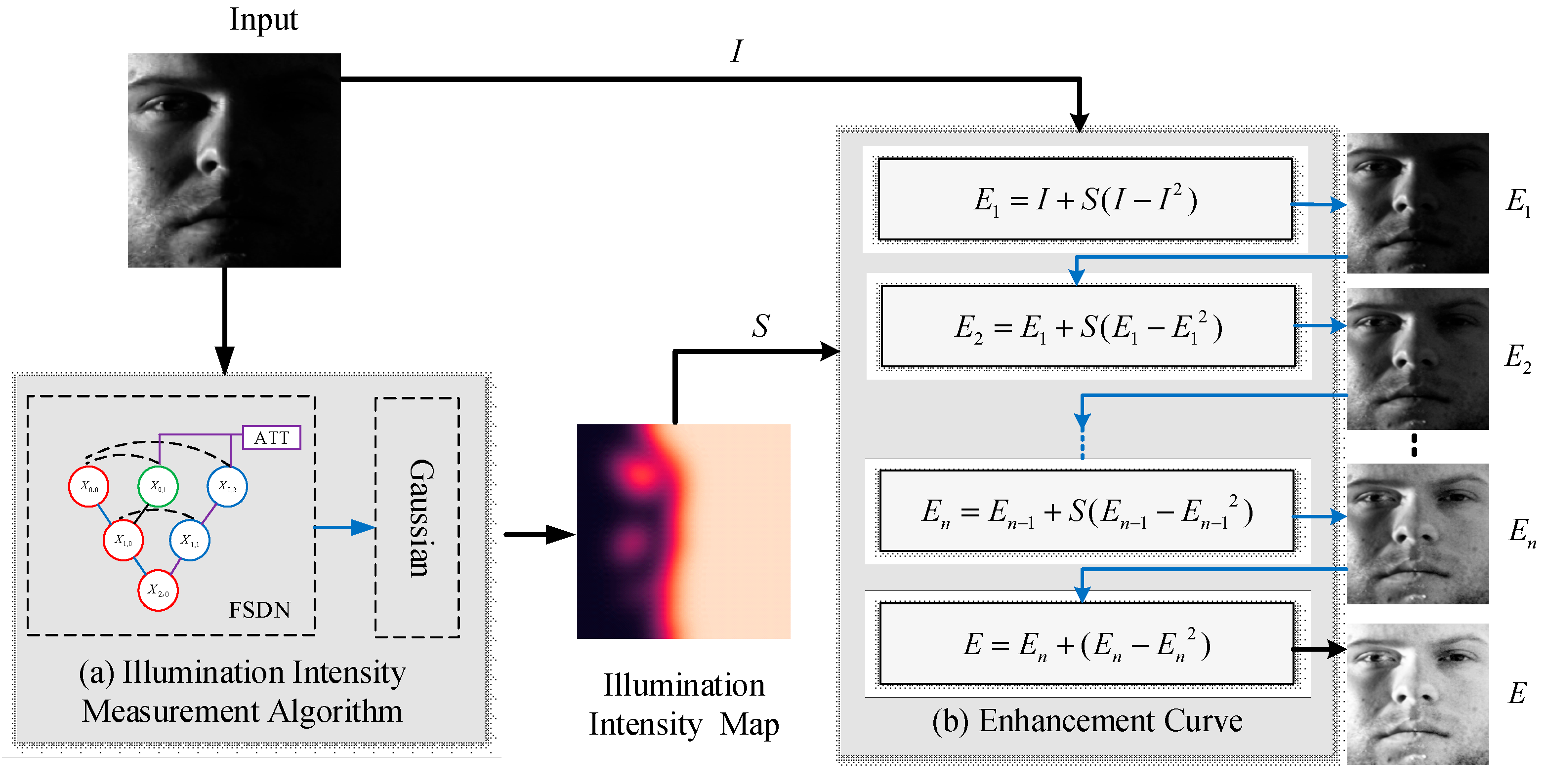
Figure 2. Face shadow detection network. (a) FSDN high-level overview. $X^{i,j}$ contains the batch normalization and the activation function. The feature dimensions of each layer are set to 64, 128, 256, 512 from top to bottom. (b) Attention module architecture.

Figure 2. Face shadow detection network. (a) FSDN high-level overview. $X^{i,j}$ contains the batch normalization and the activation function. The feature dimensions of each layer are set to 64, 128, 256, 512 from top to bottom. (b) Attention module architecture.

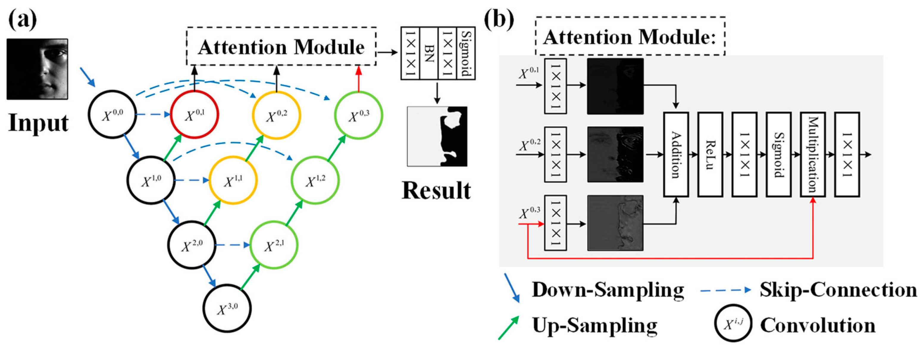
Backbone: As illustrated in Figure 2a, the nested U-Net structure based on the encoder–decoder configuration contains several secondary U-Nets with different depths. In each feature dimension, FSDN extends a decoding branch, and each branch is used to extract semantic features of different depths of the image. The image obtains several feature maps in the same size through each branch. It can be observed that the shallower branches extract more high-resolution image features, thereby improving the detection of small shadow areas. The deeper branches have a larger receptive field. Hence, more global image features can be extracted. These features help the network distinguish pixels that can be easily confused with shadow pixels, such as the pixels of eyebrows. In general, the nested U-Net structure reduces detail loss from down-sampling while maintaining a sufficient receptive field.

Network Connectivity: The skip connections in FSDN are designed to incorporate high-resolution information. This connectivity pattern is formally defined in Equation (1), where $x^{i,j}$ denotes the output of module $X^{i,j}$, $\psi ( )$ stands for the convolution operation, $U( )$ indicates the up-sampling operation, and $[ ]$ symbolizes the feature concatenation via skip connections. Specifically, if $j$ equals 0, the nodes receive only the output from the preceding encoder node. If $j$ is larger than 0, the input consists of the calculated results from the node at the current level ($x^{i,0}$), combined with the up-sampled results from the previous node ($x^{i+1,j-1}$). After the connection mentioned above, each secondary U-Net is still independent of each other, thus an attention module can be used to connect them.

$$\left\{\begin{array}{cc}{x}^{i,j}=\psi \left(x^{i-1,j}\right),\hfill & j=0\\ x^{i,j}=\psi \left(\right[x^{i,0},U\left(x^{i+1,j-1}\right)],\hfill & j>0\end{array}\right.$$

(1)

Attention Module: An attention module with multiple inputs is designed to integrate feature tensors from different branches. The attention module is shown in Figure 2b. The outputs from the deepest branch of the U-Net are selected as the primary inputs to this module, as it has the widest receptive field but hides the least noise compared to the outputs from other branches. The feature maps produced by sub-U-Nets are all put through the $1\times 1\times 1$ convolutional layer for dimensionality reduction. Then, gating coefficients ${\partial }_n\in \left[\mathrm{0,1}\right]$ are generated using an additive attention mechanism. The results obtained from the sub-U-Net with the widest receptive field are refined via dot product operations to emphasize target regions. Within the attention module, the sigmoid activation is defined as $\delta \left(x\right)=1/(1+e^{-x})$, while $\sigma$ denotes the ReLu function. Here, $W_x^i$ corresponds to linear transformations which consist of a $1\times 1\times 1$ convolutional layer, $g_i\left(x\right)$ represents the output of module $X^{0,j}(i>0)$, with $n$ indicating the number of inputs. Then, connect two $1\times 1\times 1$ convolutional filters, one batch normalization, and one sigmoid activation function to output the final shaded pixel probability map.

$$y=g_n(x)\delta (\sigma \sum _{i=1}^n{W}_x^i{g}_i\left(x\right))$$

(2)

$$Dice\_loss=1-{\displaystyle \frac{2{\sum }_i^N{p}_i{g}_i}{{\sum }_i^N{p}_i^2+{\sum }_i^N{g}_i^2+\eta }}$$

(3)

Loss Function: For facial images with uneven illumination, shadowed areas exhibit significant dimensional variations due to complex lighting conditions. In some samples, the shadowed areas are particularly small, which may easily lead to local minimums during training and cause the model to produce predictions of background bias. To address the class imbalance between useless backgrounds and shadows that need attentions, Dice_loss [42] is adopted as the loss function, which is defined in Equation (3), where the subtrahend denotes the Dice coefficient. The predicted segmentation pixels are denoted as $p_i\in P$, and the corresponding ground truth pixels are denoted as $g_i\in G$. Constant $\eta =1\times {10}^{-5}$ is used to prevent the denominator from being 0. When prediction and mask become more similar, the Dice coefficient goes towards $1$.

3.1.2. Facial Illumination Intensity Map

After being processed by a shadow detection network, the face image is divided into shadow and non-shadow areas which represent the illumination intensity level with a binary map to a certain extent. However, it is not enough to show the illumination intensity level with a binary map based on two reasons. Firstly, the shadow detection network may make mistakes. Secondly, there are half-shaded areas in the image where the illumination intensity level of the pixels is between that of the shadow area and the normal area. Therefore, the transition of illumination intensity maps should be smooth between low-light area and normal-light area. Based on the above, the illumination intensity level of a pixel in the image should also be related to whether surrounding pixels are recognized as shadows. Hence, the illumination intensity of a pixel in the image is defined as equal to the weighted sum of the shadow detection results of all pixels in a certain-sized window centered on this pixel, and the weight is negatively related to the distance from the target point. Equation (4) demonstrates the illumination intensity level, where $S_{x,y}$ is the illumination intensity value, $P_{i,j}$ is the shadow detection result with value 0 or 1, ${\alpha }_{i,j}$ is the corresponding weight, $I$ is the length of the window, and $J$ is the width of the window. Equation (5) gives the calculation process of ${\alpha }_{i,j}$. The two-dimensional normal distribution is selected to assign it, which guarantees the negative correlation between the weight and the distance, as well as ensuring that the final illumination intensity value $S_{x,y}$ is constrained to range [0, 1]. In this function, the kernel size is 3 × 3 and the $\sigma$ is set to 0.8. The $\sigma$ is automatically calculated based on the kernel size. This configuration is chosen because a 3 × 3 kernel represents a common practice that balances receptive field coverage with computational efficiency.

$$S_{x,y}=\sum _I\sum _J{\alpha }_{i,j}{P}_{i,j}$$

(4)

$${\alpha }_{i,j}={\displaystyle \frac{1}{2\pi {\sigma }^2}}{e}^{-(i^2+j^2)/2{\sigma }^2}$$

(5)

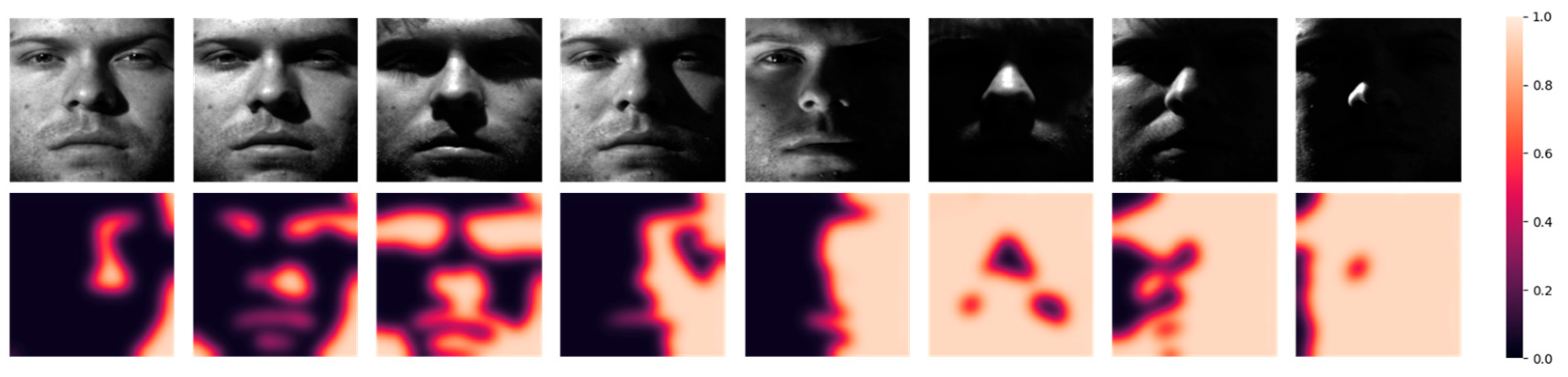
To obtain the corresponding illumination intensity map, simply perform Gaussian convolution on the shadow detection map. Figure 3 shows the illumination intensity heat maps of the example images. The darker the pixel is, the closer its intensity value is to 1. The algorithm obtains a smoother illumination intensity value at the junction of the shadow and the non-shadow area, which makes illumination intensity map more reasonable.

Figure 3. The illumination intensity heatmap in different illumination conditions. The darker the pixel is, the closer the intensity value is to 1.

3.2. Illumination Enhancement Curve

A solution is designed to personalize each pixel in the face image according to the illumination intensity map. Inspired by Zero-DCE [18], higher-order quadratic curve is employed for image enhancement. This curve has the following features: (1) The pixel value range of the normalized image after enhancement is [0, 1] to avoid information loss caused by truncation; (2) The curve should be monotonically increasing to achieve the exposure; (3) Each pixel in the image should correspond to an exposure level control value to adapt to complex illumination conditions. Equation (6) is the mathematical expression of the designed enhancement curve. Among them, $I_{x,y}\in [0, 1]$ is the normalized original pixel value, $S_{x,y}\in [0, 1]$ is the exposure level control value which is taken from the illumination intensity map obtained in Section 3.1, and $E_{x,y}$ is the enhanced pixel value.

$$E_{x,y}=I_{x,y}+S_{x,y}(I_{x,y}-{I_{x,y}}^2)$$

(6)

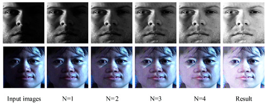
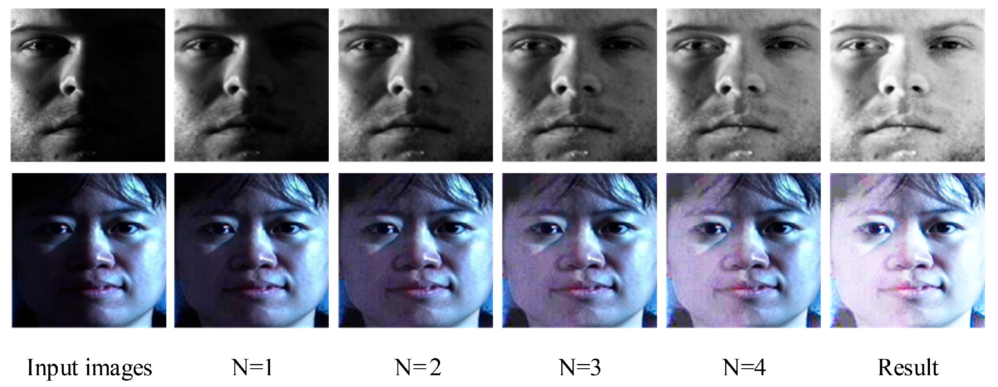
The above enhancement curve can iteratively process the image to adapt to extreme illumination conditions. The following iterative plan is recommended for enhancing face images. Firstly, use Equation (6) to perform N iterations of image enhancement. Then, set the exposure level control map $S$ to 1 and perform an enhancement. The main purpose of this step is to unify the overall exposure level. The iterative enhancement of the whole image can be described by Equations (7) and (8), where $E_n$ is the enhancement result after iterations, $S$ is the illumination intensity map, and $E$ is the image processed by the algorithm. Since $E_n\in [0, 1]$, the three features of the higher-order curve remain there. For color images, the curve is applied to the three channels, respectively, to obtain the final enhancement result. Figure 4 shows the iterative enhancement process which illustrates that the brightness of the dark areas in the image gradually increases with the increasing iterations.

$$E_n=E_{n-1}+S(E_{n-1}-{E_{n-1}}^2)$$

(7)

$$E=2E_n-{E_n}^2$$

(8)

Figure 4. The iterative enhancement process.

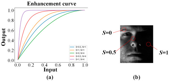
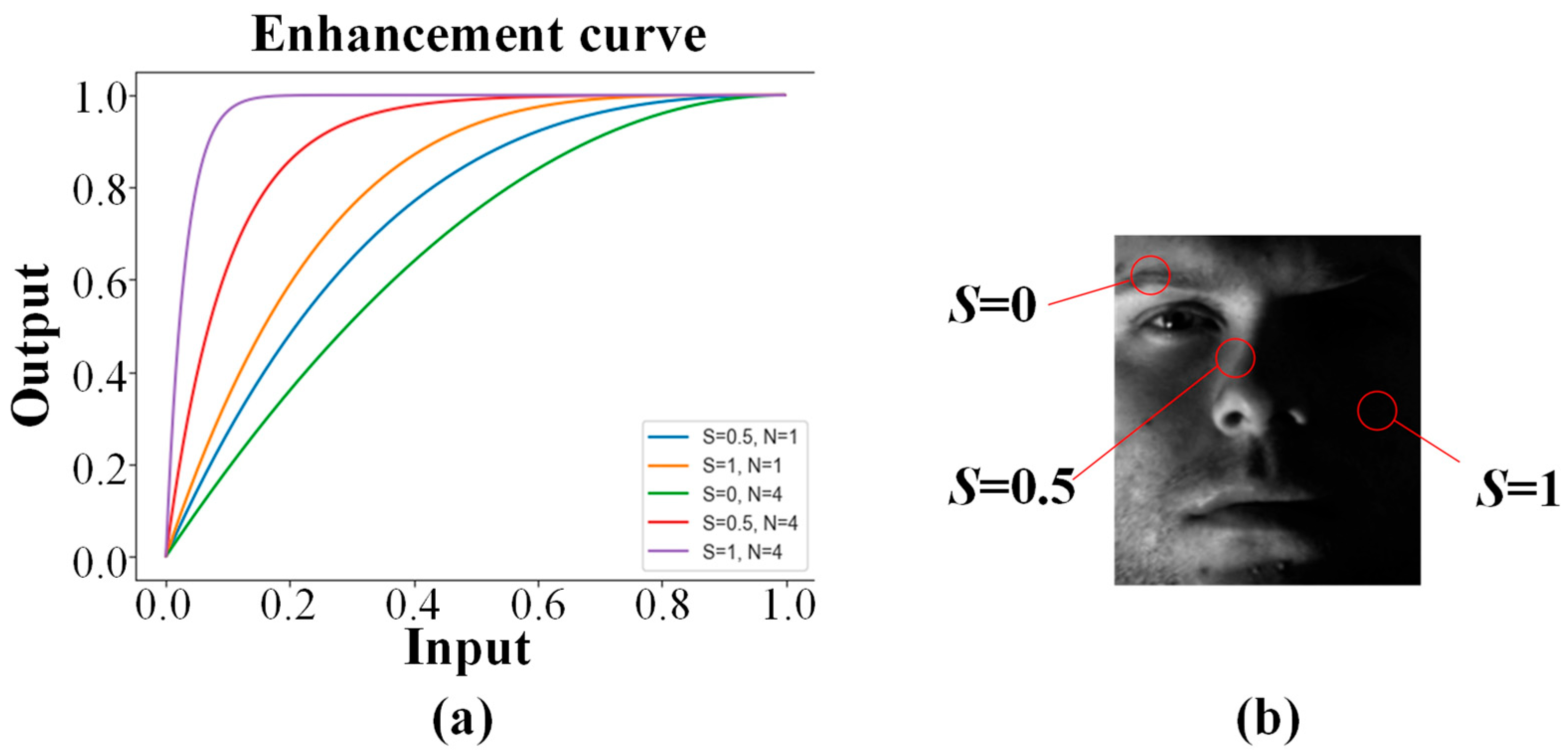
Through the control of the illumination intensity map, each pixel in the image has been enhanced to different degrees, the illumination of the low-light area in the image is restored, and the structure of the area with normal light is also better saved. Figure 5a shows the enhancement curves with different exposure control parameters and the number of iterations. As shown in Figure 5b, the number of iterations is set to 4, which is based on empirical value. The pixels in low-light areas are assigned to a higher exposure control parameter and mapped to a wider dynamic range through the purple curve, thus achieving illumination enhancement. For the normal areas, the enhancement curve represented by the green curve is close to $E=I$, which only slightly changes the pixel value. In addition, the overall smooth exposure control values make the exposure level in a certain area consistent or change slowly, which helps to ensure the monotonic relationship between neighboring pixels in the area.

Figure 5. (a) Enhancement curve, the horizontal axis is the input value I, while the vertical axis is the output value $E$. $S$ is the exposure control parameter and N is the number of iterations. (b) The pixels in each area of the image are assigned to different exposure control values according to the illumination intensity map.

4. Results

The experiment comprises two main parts: the evaluation of FSDN and the analysis of the illumination enhancement results.

4.1. Dataset

Face shadow detection dataset: The face shadow detection dataset for the work of shadow detection is created. Frontal face images containing low-light or shadow areas were selected from the Extended Yale B face database, with the shadow areas subsequently marked out using Labelme. The whole dataset comprises over 1600 pairs of face images and corresponding shadow masks, utilized for both training and evaluating the face shadow detection network.

Extended Yale B [23]: This dataset comprises 38 subjects, with each subject captured under 64 different lighting conditions. In the case of harsh illumination, the face structure in the low-light area cannot be seen with the naked eye.

CMU-PIE [22]: There are 41,368 color images of 68 volunteers in the dataset, and the postures, illumination conditions, and facial expressions are all different. The experimental data consisted of frontal pose face images from the illumination subset of the dataset, comprising 68 subjects across 19 distinct illumination conditions.

4.2. Implementation Details

Face shadow detection: The created face shadow detection dataset is divided into a training set and a test set according to the ratio 3:1. The test and training sets are randomly split while ensuring coverage of all illumination conditions as much as possible. To verify the superiority of FSDN, comparative experiments were conducted against several established models, namely U-Net [43], U-Net++ [44], and OC-RNet [45], as well as two recently developed shadow detection networks: DSD [40] and BDRAR [38]. For FSDN, the Adam optimizer [46] is deployed, with the learning rate of 0.0001 and the batch size of 8. All deep networks are trained for 50 epochs with RTX 2070S GPU.

Face image illumination enhancement: Two classic illumination enhancement methods He [4], MSR (MSRCR) [8] are adopted in the comparative experiment, and the current more advanced deep-learning-based methods Retinex-Net [15] and Zero-Dce [18] are set as the control group. For deep learning-based approaches, the dataset is divided into training and test set at a 4:1 ratio according to the individual differences. In the proposed method, shadow masks for all face images across both datasets are generated using the pre-trained FSDN model, after which the process advances to the subsequent stage. The number of curve iterations is set to 4. For each person, the image with frontal uniform illumination is selected as the ground truth.

4.3. Results of Face Shadow Detection

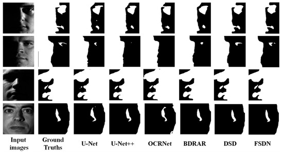
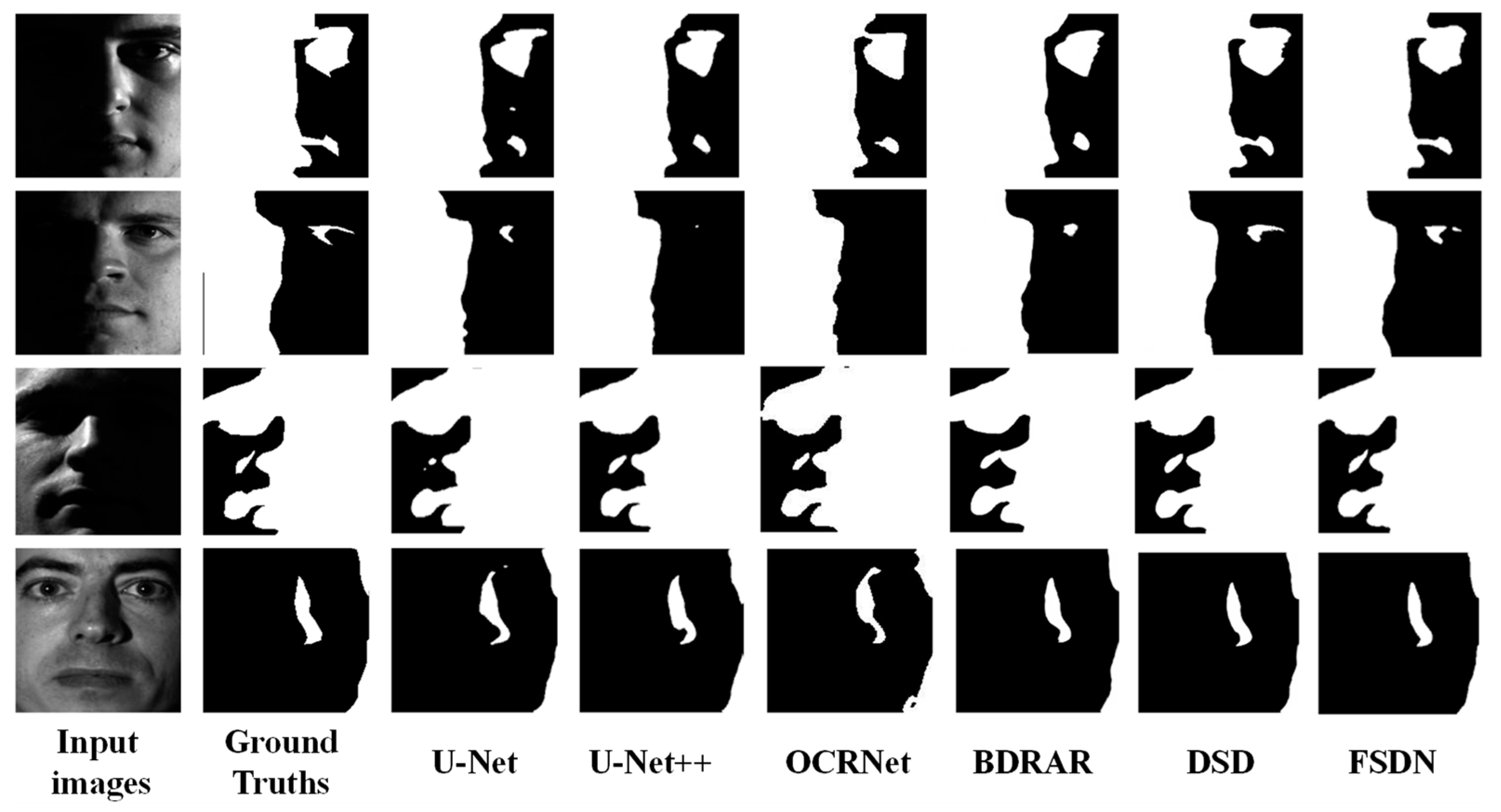
As shown in Figure 6, visual comparison is conducted between the face shadow detection maps produced by the proposed method and others. From the visual results, it can be seen that FSDN achieves the best results and effectively located shadow areas in various sizes. However, the classic segmentation network and BDRAR are not effective in detecting small shadow targets and make more mistakes in shadow edge positioning. For instance, only DSD and FSDN successfully detected the shadow around the eyes in the second example image. Similarly, as can be seen from the results in the fourth column, the results of DSD and FSDN are closer to the true value, with more accurate shadow edges.

Figure 6. Face shadow detection results.

A quantitative analysis of each method’s results is conducted. In this evaluation, three metrics are employed: IoU, shadow error rate (SER), non-shadow error rate (NER), and their balanced combination (BER) to comprehensively assess network performance [40]. The calculation of IoU, SER, NER, and BER is defined in Equations (9)–(12), respectively.

$$\mathrm{IoU}={\displaystyle \frac{\mathrm{Ground}\_\mathrm{Truth}\cap \mathrm{Prediction}}{\mathrm{Ground}\_\mathrm{Truth}\cup \mathrm{Prediction}}}$$

(9)

$$\mathrm{SER}=(1-N_{tp}/N_p)\times 100$$

(10)

$$\mathrm{NER}=(1-N_{tn}/N_n)\times 100$$

(11)

$$\mathrm{BER}=(\mathrm{SER}+\mathrm{NER})/2$$

(12)

where $N_{tp}$ and $N_{tn}$ denote the number of correctly predicted shadow and correctly predicted non-shadow pixels, respectively, while $N_p$ and $N_n$ represent the total number of actual shadow and non-shadow pixels.

Table 1 summarizes the quantitative performance of all evaluated methods. The results indicate that the classic image segmentation network in shadow detection is less satisfactory. Compared with the best performing DSD in the comparison group, FSDN performs better in IoU, SER, and BER IoU increased 1.0%, BER decreased by 29.8%, and SER decreased by 14.2%. Based on visual and quantitative results, the nested structure of FSDN effectively mitigates information loss from down-sampling, allowing the network to accurately detect small shadow areas while lowering the BER.

Table 1. Comparing FSDN to the other shadow detectors.

Methods	IoU	SER	NER	BER
U-Net [43]	0.84	8.06	5.15	6.61
U-Net++ [44]	0.84	7.92	4.97	6.45
OCRNet [45]	0.83	8.98	4.83	6.91
BDRAR [38]	0.86	8.06	5.15	6.61
DSC [47]	0.83	8.67	3.67	6.21
DSD [40]	0.91	4.36	2.50	3.43
FSDN	0.92	3.06	2.81	2.94

4.4. Illumination Enhancement Results

4.4.1. Qualitative Results

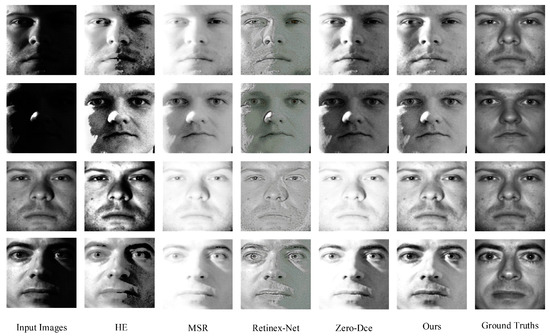
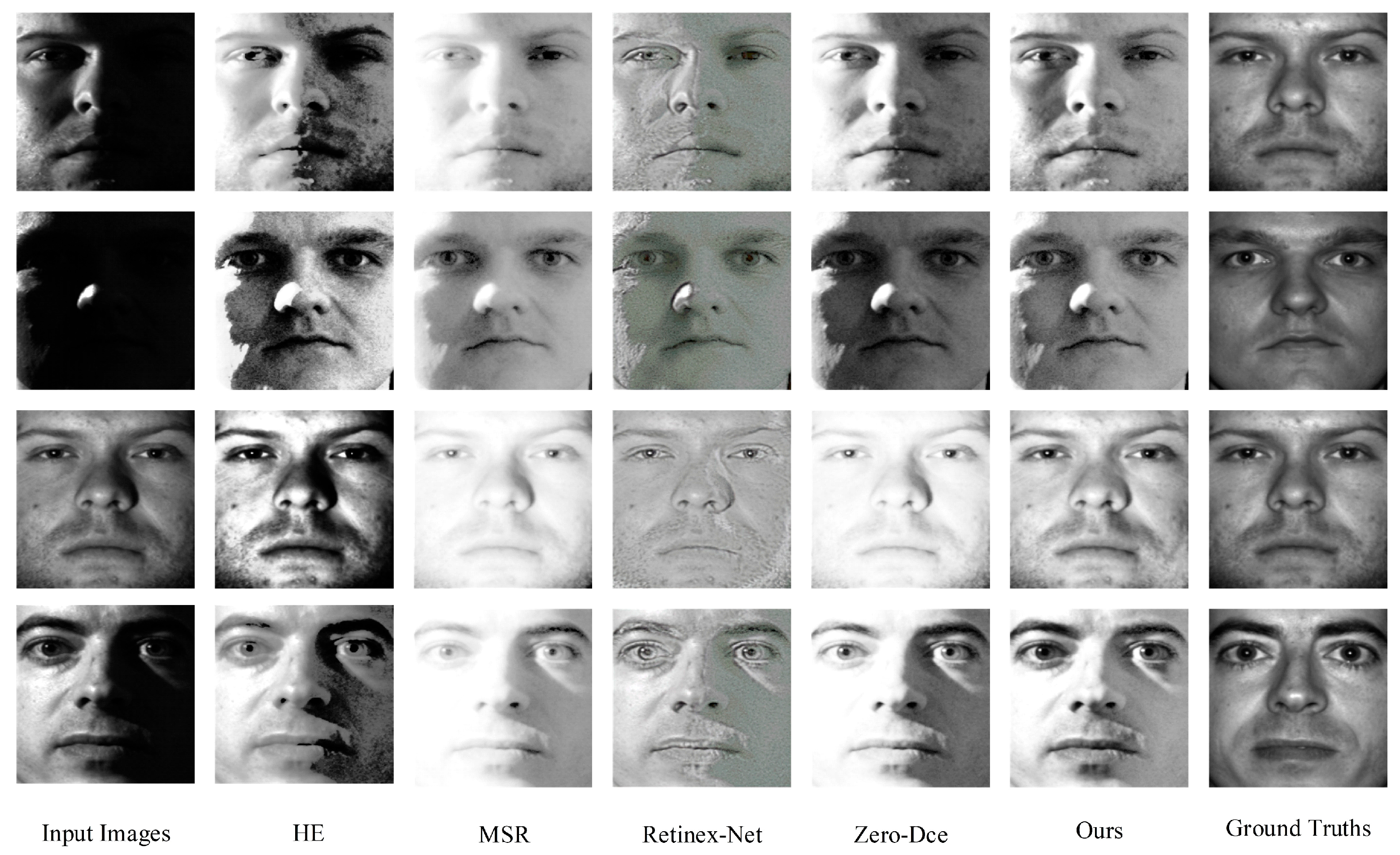
Figure 7 shows the results of the algorithm when processing gray face images in which the last column is the reference image.

Figure 7. Illumination enhancement for images in different illumination conditions from the Extended Yale B database.

According to the results, HE enhances overall image contrast, but it fails to restore details in low-light areas when the image has a wide dynamic range. The MSR successfully restores the structure of the low-light areas, but the halo caused by the enhancement greatly affects the visual performance. In addition, the processed images are transitionally smooth, resulting in the loss of a large amount of face details. Although the Retinex-Net successfully restores the structure of the low-light areas, more noise and obvious shadow false edges appear in the processed image. The original illumination change pattern is kept in the image processed by Zero-Dce. Although the low-light areas are relighted, normal areas in the image are overexposed, resulting in the loss of face details in the normal areas of the image. After using a meticulously designed exposure control value, although an enhancement curve similar to Zero-Dce being adopted, the enhancement result keeps more face detail information and changes the overall illumination distribution of the image, thereby adjusting it closer to real value. This is because the proposed method establishes a more reasonable curve mapping relationship. The method pays more attention to stretching its dynamic range when processing low-light pixels, as shown by the purple curve in Figure 5a. When processing the normal area, the method inclines to maintain its original pixel dynamic range, as shown in the mapping relationship shown by the green curve in Figure 5a.

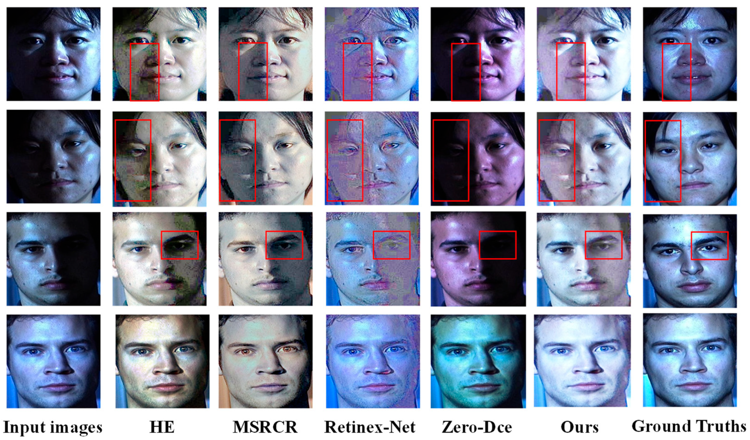
Figure 8 shows the results of the color image processing. The color deviation in HE and MSRCR is obvious. The result of Reinex-Net model still shows a lot of noise, and the relighting in the low-light areas did not work well. Zero-Dce seems to have failed on the color image enhancement. As to the method in this paper, the processed color images kept more detailed information and maintained the color closer to the true value.

Figure 8. Illumination enhancement for images from the CMU-PIE database.

4.4.2. Quantitative Results

In this part, the SSIM [48] and face recognition error rate are adopted to measure the quantitative performance of the methods. All images included in the datasets have been tested, and their average values are taken as the final score. SSIM is a commonly used metric for measuring the structural similarity between two images. It is considered to be correlative with the quality perception of the human visual system. SSIM compares the luminance, contrast, and the structure of the two images. The calculation of SSIM is shown in Equation (13), where ${\mu }_x$ is the average of $x$, ${\mu }_y$ is the average of $y$, ${\sigma }_x$ is the variance of $x$, ${\sigma }_y$ is the variance of $y$, and ${\sigma }_{xy}$ is the covariance of $x$ and $y$. For the Extended Yale database, it can be seen from Table 2 that the result processed by HE is the least similar one to the ground truth due to the failed processing of HE on the samples with severe lighting changes. The scores of the data-driven methods are also low. Although the exposure level of the image processed by Retinex-Net is close to the ground truth, there is an obvious gap between their structures due to the false edge. The result processed by Zero-Dce is far from the ground truth in terms of brightness, which resulted in its lower SSIM. The SSIM of MSR is slightly lower than the proposed method. This is because some detailed information is lost.

$$\mathrm{SSIM}(x,y)={\displaystyle \frac{(2{\mu }_x{\mu }_y+c_1)(2{\sigma }_{xy}+c_2)}{({{\mu }_x}^2+{{\mu }_y}^2+c_1)({{\sigma }_x}^2+{{\sigma }_y}^2+c_2)}}$$

(13)

Table 2. Comparisons between different methods for SSIM and face recognition error rate (%) on two databases.

Methods	SSIM		Face Recognition Error Rate (%)
	Yale B	CMU-PIE	Yale B	CMU-PIE
HE	0.42	0.54	2.9	0.3
MSR (MSRCR)	0.47	0.54	4.74	0.2
Retinex-Net	0.45	0.53	6.56	0.4
Zero-Dce	0.44	0.58	1.3	0.3
This work	0.48	0.59	1.3	0.2

For the CMU-PIE, the SSIM in the results is higher. This is because the illumination in the CMU-PIE is equal to or less extreme than that of Extended Yale B. It is worth noting that although Zero-Dce almost failed on CMU-PIE in the qualitative analysis, it still achieves a higher SSIM. The reason is that although the Zero-Dce cannot successfully restore the structures of the low-light areas, it well preserves the structures of the normal light areas. Due to the non-extreme illumination, the face image in the CMU-PIE contains many normal illumination areas, so that the SSIM processed by Zero-Dce can still be maintained at a high level.

In the experiment of face recognition, the frontal normal illumination image of each individual is registered as a gallery image, and the image in various illumination conditions is regarded as a detection image. The pre-trained VGG-Face2 model [49] is adopted to extract feature vectors from both the detected image and gallery face, with the cosine distance between these vectors serving as the identity similarity metric. The distance threshold is set to 0.5. When the cosine distance is shorter than 0.5, the two images are recognized as the same person. Table 2 shows the error rate of face recognition. In the Extended Yale B dataset, the experimental results demonstrate that various illumination recovery methods have improved the accuracy of face recognition. Both Zero-Dce and the proposed method have achieved high detection accuracy. Although the exposure level of the dark areas processed by Zero-Dce is low, VGG-Face2 is robust enough to adapt to this change. Other methods will lose more face structure information, which will lead to a decrease in recognition accuracy. In addition, in the CMU-PIE dataset, since the illumination of the face images contained in the database is not extreme, the error rates of face recognition are all at a low level.

4.4.3. Ablation Study

Ablation experiments of two datasets are set up to verify the effectiveness of each module of the algorithm, including removing the exposure control parameter and the Gaussian smoothing of the shadow detection map (using the shadow detection map directly as the exposure control parameter).

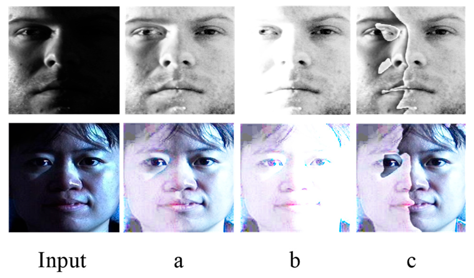
Figure 9b shows the enhancement result after removing the exposure control parameter. After the global iterative enhancement of the image, the normal-light areas are overexposed, causing the loss of most face structure information in the areas. Figure 9c is the enhancement result of directly using the shadow detection map as the exposure control parameter. The enhanced image changes drastically at the junction of the low-light and normal-light areas, forming an unbearable false edge. Table 3 shows the quantitative results of the ablation study, further verifying the necessity of each operation in the method. After removing the exposure control parameter, SSIM is reduced by 20.8% and 40.0%, and the face recognition error rate is increased by 400% and 370% of Extended Yale B and CMU-PIE, respectively. After removing the Gaussian smoothing process on the shadow detection map, SSIM is reduced by 8.3% and 40.1%, and the face recognition error rate is increased by 153% and 0% of Extended Yale B and CMU-PIE, respectively.

Figure 9. The ablation study results. (a) Results of the proposed method. (b) Results without exposure control parameter. (c) Using the shadow detection map directly as the exposure control parameter.

Table 3. Comparisons between different databases for SSIM and face recognition rate (%) of ablation study.

Loss Term	SSIM		Face Recognition Error Rate (%)
	Yale B	CMU-PIE	Yale B	CMU-PIE
$\mathrm{w}/\mathrm{o} S_{x,y}$	0.38	0.35	0.542	37.2
w/o Gaussian smoothing	0.44	0.54	0.033	0.2

5. Conclusions

A novel symmetry-aware face illumination enhancement method is proposed, which effectively solves the challenging problem of uneven illumination in face image applications. In the solution of this work, the face shadow detection map is first obtained through the face shadow detection network, then processed by Gaussian smoothing to obtain the face illumination intensity map. The quadratic curve using the illumination intensity map as the exposure control parameter is iteratively applied to the enhancement. Experimental results indicate that the proposed FSDN works better than the current advanced shadow detection methods. In addition, the illumination enhancement contrast experiment also shows that the proposed method greatly improves the accuracy of face recognition under extreme illumination, and more face detail information can be kept in the processed image. The method proves particularly effective in correcting asymmetric illumination while respecting the inherent symmetry of facial structures. Comprehensive evaluations on the Extended Yale B and CMU-PIE datasets demonstrate the superiority of the proposed FSDN over conventional approaches, achieving SSIM indices of 0.48 and 0.59, respectively, along with remarkably low face recognition error rates of 1.3% and 0.2%, respectively.

In conclusion, the proposed method significantly advances low-light face image enhancement by improving Zero-DCE’s illumination restoration curve through two novel exposure control parameters derived from facial shadow detection and illumination direction analysis. Extensive experiments on Extended Yale B and CMU-PIE datasets demonstrate their superior performance in restoring facial structures in dark regions while preserving texture details in well-lit areas, achieving both lower color deviation and higher face recognition accuracy than comparative methods.

The proposed method, however, has limitations in two key aspects. First, the technique demonstrates reduced effectiveness in restoring low-light regions occluded by facial structures such as the nose, often resulting in residual shadows and pseudo-edge artifacts in the processed images. Future research will focus on generating and compensating for these occluded facial structures to address this limitation. Second, the current algorithm’s performance in illumination restoration across varying facial poses remains suboptimal, indicating a need for additional research to improve pose-invariant illumination adjustment. These limitations highlight important directions for future work to enhance the method’s robustness and applicability in real-world scenarios where facial occlusions and pose variations are common.

References

- Adini, Y.; Moses, Y.; Ullman, S. Face recognition: The problem of compensating for changes in illumination direction. IEEE Trans. Pattern Anal. Mach. Intell. 1997, 19, 721–732. [Google Scholar] [CrossRef] [Scilit]
- Emadi, M.; Khalid, M.; Yusof, R.; Navabifar, F. Illumination normalization using 2D wavelet. Procedia Eng. 2012, 41, 854–859. [Google Scholar] [CrossRef] [Scilit]
- Chen, W.; Er, M.J.; Wu, S. Illumination compensation and normalization for robust face recognition using discrete cosine transform in logarithm domain. IEEE Trans. Syst. Man Cybern. Part B (Cybern.) 2006, 36, 458–466. [Google Scholar] [CrossRef] [Scilit] [PubMed]
- Pizer, S.M.; Amburn, E.P.; Austin, J.D.; Cromartie, R.; Geselowitz, A.; Greer, T.; ter Haar Romeny, B.; Zimmerman, J.B.; Zuiderveld, K. Adaptive histogram equalization and its variations. Comput. Vis. Graph. Image Process. 1987, 39, 355–368. [Google Scholar] [CrossRef] [Scilit]
- Xie, X.; Lam, K.-M. Face recognition under varying illumination based on a 2D face shape model. Pattern Recognit. 2005, 38, 221–230. [Google Scholar] [CrossRef]
- Xie, X.; Lam, K.-M. An Efficient Method for Face Recognition Under Varying Illumination. In Proceedings of the 2005 IEEE International Symposium on Circuits and Systems, Kobe, Japan, 23–26 May 2005; pp. 3841–3844. [Google Scholar]
- Xie, X.; Lam, K.-M. An efficient illumination normalization method for face recognition. Pattern Recognit. Lett. 2006, 27, 609–617. [Google Scholar] [CrossRef] [Scilit]
- Vishwakarma, V.P.; Pandey, S.; Gupta, M.N. Adaptive histogram equalization and logarithm transform with rescaled low frequency DCT coefficients for illumination normalization. Int. J. Recent Trends Eng. 2009, 1, 318. [Google Scholar]
- Lee, P.-H.; Wu, S.-W.; Hung, Y.-P. Illumination compensation using oriented local histogram equalization and its application to face recognition. IEEE Trans. Image Process. 2012, 21, 4280–4289. [Google Scholar] [CrossRef] [Scilit]
- Basri, R.; Jacobs, D. Lambertian reflectance and linear subspaces. IEEE Trans. Pattern Anal. Mach. Intell. 2003, 25, 218–233. [Google Scholar] [CrossRef] [Scilit]
- Xie, X.; Zheng, W.-S.; Lai, J.; Yuen, P.C.; Suen, C.Y. Normalization of face illumination based on large-and small-scale features. IEEE Trans. Image Process. 2010, 20, 1807–1821. [Google Scholar] [CrossRef] [Scilit]
- Matsukawa, T.; Okabe, T.; Sato, Y. Illumination Normalization of Face Images with Cast Shadows. In Proceedings of the 21st International Conference on Pattern Recognition (ICPR2012), Tsukuba, Japan, 11–15 November 2012; pp. 1848–1851. [Google Scholar]
- Lore, K.G.; Akintayo, A.; Sarkar, S. LLNet: A deep autoencoder approach to natural low-light image enhancement. Pattern Recognit. 2017, 61, 650–662. [Google Scholar] [CrossRef] [Scilit]
- Shen, L.; Yue, Z.; Feng, F.; Chen, Q.; Liu, S.; Ma, J. Msr-net: Low-light image enhancement using deep convolutional network. arXiv 2017, arXiv:1711.02488. [Google Scholar]
- Wei, C.; Wang, W.; Yang, W.; Liu, J. Deep retinex decomposition for low-light enhancement. arXiv 2018, arXiv:1808.04560. [Google Scholar] [CrossRef] [Scilit]
- Zhang, Y.; Zhang, J.; Guo, X. Kindling the darkness: A practical low-light image enhancer. In Proceedings of the 27th ACM International Conference on Multimedia, Nice, France, 21–25 October 2019; Association for Computing Machinery: New York, NY, USA, 2019; pp. 1632–1640. [Google Scholar]
- Jiang, Y.; Gong, X.; Liu, D.; Cheng, Y.; Fang, C.; Shen, X.; Yang, J.; Zhou, P.; Wang, Z. Enlightengan: Deep light enhancement without paired supervision. IEEE Trans. Image Process. 2021, 30, 2340–2349. [Google Scholar] [CrossRef] [Scilit] [PubMed]
- Guo, C.; Li, C.; Guo, J.; Loy, C.C.; Hou, J.; Kwong, S.; Cong, R. Zero-Reference Deep Curve Estimation for Low-Light Image Enhancement. In Proceedings of the IEEE/CVF Conference on Computer Vision and Pattern Recognition, Seattle, WA, USA, 13–19 June 2020; pp. 1777–1786. [Google Scholar]
- Xie, C.; Fei, L.; Tao, H.; Hu, Y.; Zhou, W.; Hoe, J.T.; Hu, W.; Tan, Y.-P. Residual quotient learning for zero-reference low-light image enhancement. IEEE Trans. Image Process. 2025, 34, 365–378. [Google Scholar] [CrossRef] [Scilit]
- Yu, C.; Han, G.; Pan, M.; Wu, X.; Deng, A. Zero-tce: Zero reference tri-curve enhancement for low-light images. Appl. Sci. 2025, 15, 701. [Google Scholar] [CrossRef] [Scilit]
- Yan, Q.; Feng, Y.; Zhang, C.; Pang, G.; Shi, K.; Wu, P.; Dong, W.; Sun, J.; Zhang, Y. HVI: A new color space for low-light image enhancement. arXiv 2025, arXiv:2502.20272. [Google Scholar]
- Sim, T.; Baker, S.; Bsat, M. The CMU Pose, Illumination, and Expression (PIE) Database. In Proceedings of the fifth IEEE International Conference on Automatic Face Gesture Recognition, Washington, DC, USA, 21 May 2002; pp. 53–58. [Google Scholar]
- Georghiades, A.S.; Belhumeur, P.N.; Kriegman, D.J. From few to many: Illumination cone models for face recognition under variable lighting and pose. IEEE Trans. Pattern Anal. Mach. Intell. 2001, 23, 643–660. [Google Scholar] [CrossRef] [Scilit]
- Finlayson, G.D.; Hordley, S.D.; Lu, C.; Drew, M.S. On the removal of shadows from images. IEEE Trans. Pattern Anal. Mach. Intell. 2005, 28, 59–68. [Google Scholar] [CrossRef] [Scilit]
- Finlayson, G.D.; Drew, M.S.; Lu, C. Entropy minimization for shadow removal. Int. J. Comput. Vis. 2009, 85, 35–57. [Google Scholar] [CrossRef] [Scilit]
- Guo, R.; Dai, Q.; Hoiem, D. Single-image shadow detection and removal using paired regions. In Proceedings of the 2011 IEEE Conference on Computer Vision and Pattern Recognition, Colorado Springs, CO, USA, 20–25 June 2011; pp. 2033–2040. [Google Scholar]
- Guo, R.; Dai, Q.; Hoiem, D. Paired regions for shadow detection and removal. IEEE Trans. Pattern Anal. Mach. Intell. 2012, 35, 2956–2967. [Google Scholar] [CrossRef] [Scilit]
- Vicente, T.F.Y.; Yu, C.-P.; Samaras, D. Single Image Shadow Detection Using Multiple Cues in a Supermodular MRF. In Proceedings of the British Machine Vision Conference, Bristol, UK, 9–13 September 2013. [Google Scholar]
- Yuan, X.; Ebner, M.; Wang, Z. Single-image shadow detection and removal using local colour constancy computation. IET Image Process. 2015, 9, 118–126. [Google Scholar] [CrossRef] [Scilit]
- Liu, J.; Tang, Q.; Wang, Y.; Lu, Y.; Zhang, Z. Defects’ geometric feature recognition based on infrared image edge detection. Infrared Phys. Technol. 2014, 67, 387–390. [Google Scholar] [CrossRef] [Scilit]
- Hamza, S.A.; Jesser, A. A study on advancing Edge Detection and Geometric Analysis through Image Processing. In Proceedings of the 2024 8th International Conference on Graphics and Signal Processing (ICGSP ’24), Tokyo, Japan, 14–16 June 2024; Association for Computing Machinery: New York, NY, USA, 2024; pp. 9–13. [Google Scholar]
- Yang, D.; Peng, B.; Al-Huda, Z.; Malik, A.; Zhai, D. An overview of edge and object contour detection. Neurocomputing 2022, 488, 470–493. [Google Scholar] [CrossRef] [Scilit]
- Khan, S.H.; Bennamoun, M.; Sohel, F.; Togneri, R. Automatic Feature Learning for Robust Shadow Detection. In Proceedings of the 2014 IEEE Conference on Computer Vision and Pattern Recognition (CVPR 2014), Columbus, OH, USA, 23–28 June 2014; pp. 1939–1946. [Google Scholar]
- Vicente, T.F.Y.; Hou, L.; Yu, C.P.; Hoai, M.; Samaras, D. Large-scale training of shadow detectors with noisily-annotated shadow examples. In European Conference on Computer Vision (ECCV 2016), Amsterdam, The Netherlands, 11–14 October 2016; Springer: Cham, Switzerland, 2016. [Google Scholar]
- Hosseinzadeh, S.; Shakeri, M.; Zhang, H. Fast Shadow Detection from a Single Image Using a Patched Convolutional Neural Network. In Proceedings of the 2018 IEEE/RSJ International Conference on Intelligent Robots and Systems (IROS 2018), Madrid, Spain, 1–5 October 2018; pp. 3124–3129. [Google Scholar]
- Nguyen, V.; Vicente, T.F.Y.; Zhao, M.; Hoai, M.; Samaras, D. Shadow Detection with Conditional Generative Adversarial Networks. In Proceedings of the IEEE International Conference on Computer Vision (ICCV 2017), Venice, Italy, 22–29 October 2017; pp. 4520–4528. [Google Scholar]
- Le, H.; Vicente, T.F.Y.; Nguyen, V.; Hoai, M.; Samaras, D. A+D net: Training a shadow detector with adversarial shadow attenuation. In Proceedings of the European Conference on Computer Vision (ECCV 2018), Munich, Germany, 8–14 September 2018. [Google Scholar]
- Zhu, L.; Deng, Z.; Hu, X.; Fu, C.-W.; Xu, X.; Qin, J.; Heng, P.-A. Bidirectional feature pyramid network with recurrent attention residual modules for shadow detection. In Proceedings of the European Conference on Computer Vision (ECCV 2018), Munich, Germany, 8–14 September 2018. [Google Scholar]
- Zhou, H.; Yi, J. FFSDF: An improved fast face shadow detection framework based on channel spatial attention enhancement. J. King Saud Univ. Comput. Inf. Sci. 2023, 35, 101766. [Google Scholar] [CrossRef] [Scilit]
- Zheng, Q.; Qiao, X.; Cao, Y.; Lau, R.W. Distraction-Aware Shadow Detection. In Proceedings of the IEEE/CVF Conference on Computer Vision and Pattern Recognition (CVPR 2019), Long Beach, CA, USA, 15–20 June 2019; pp. 5162–5171. [Google Scholar]
- Zhang, J.; Li, F.; Zhang, X.; Cheng, Y.; Hei, X. Multi-Task Mean Teacher Medical Image Segmentation Based on Swin Transformer. Appl. Sci. 2024, 14, 2986. [Google Scholar] [CrossRef] [Scilit]
- Shi, P.; Hu, J.; Yang, Y.; Gao, Z.; Liu, W.; Ma, T. Centerline boundary dice loss for vascular segmentation. In Proceedings of Medical Image Computing and Computer Assisted Intervention—MICCAI 2024; Springer Nature: Cham, Switzerland, 2024; pp. 46–56. [Google Scholar]
- Ronneberger, O.; Fischer, P.; Brox, T. U-net: Convolutional networks for biomedical image segmentation. In Proceedings of the International Conference on Medical Image Computing and Computer-Assisted Intervention (MICCAI 2015), Munich, Germany, 5–9 October 2015; Springer: Cham, Switzerland, 2015. [Google Scholar]
- Aadarsh, Y.G.; Singh, G. Comparing UNet, UNet++, FPN, PAN and Deeplabv3+ for Gastrointestinal Tract Disease Detection. In Proceedings of the 2023 International Conference on Evolutionary Algorithms and Soft Computing Techniques (EASCT), Bengaluru, India, 20–21 October 2023; pp. 1–7. [Google Scholar]
- Yuan, Y.; Chen, X.; Wang, J. Object-contextual representations for semantic segmentation. In Proceedings of the Computer Vision-ECCV 2020: 16th European Conference, Glasgow, UK, 23–28 August 2020; Proceedings, Part VI. Springer International Publishing: Cham, Switzerland, 2020. [Google Scholar]
- Kingma, D.P.; Ba, J. Adam: A method for stochastic optimization. arXiv 2014, arXiv:1412.6980. [Google Scholar]
- Chollet, F. Xception: Deep Learning with Depthwise Separable Convolutions. In Proceedings of the 2017 IEEE Conference on Computer Vision and Pattern Recognition, Honolulu, HI, USA, 21–26 July 2017; pp. 1800–1807. [Google Scholar]
- Bakurov, I.; Buzzelli, M.; Schettini, R.; Castelli, M.; Vanneschi, L. Structural similarity index (SSIM) revisited: A data-driven approach. Expert Syst. Appl. 2022, 189, 116087. [Google Scholar] [CrossRef] [Scilit]
- Cao, Q.; Shen, L.; Xie, W.; Parkhi, O.M.; Zisserman, A. VGGFace2: A Dataset for Recognising Faces Across Pose and Age. In Proceedings of the 13th IEEE International Conference on Automatic Face & Gesture Recognition (FG 2018), Xi’an, China, 15–19 May 2018; pp. 67–74. [Google Scholar]
Disclaimer/Publisher’s Note: The statements, opinions and data contained in all publications are solely those of the individual author(s) and contributor(s) and not of MDPI and/or the editor(s). MDPI and/or the editor(s) disclaim responsibility for any injury to people or property resulting from any ideas, methods, instructions or products referred to in the content. |
© 2025 by the authors. Licensee MDPI, Basel, Switzerland. This article is an open access article distributed under the terms and conditions of the Creative Commons Attribution (CC BY) license (https://creativecommons.org/licenses/by/4.0/).