A New Method Based on Hierarchical Belief Rule Base with Balanced Accuracy and Interpretability for Stock Price Trend Prediction

Abstract

The prediction of stock price trends is of vital importance for maintaining the stability of the financial market, optimizing resource allocation and preventing systemic risks. To ensure the practical application value of the prediction model, it is necessary to maintain prediction accuracy while ensuring that the output results of the model are interpretable, enabling decision-makers to understand and verify the prediction basis. Belief Rule Base (BRB) models, grounded in IF-THEN rule semantics, offer inherent interpretability. However, optimizing BRB models can erode this interpretability, and they are susceptible to combinatorial explosion in multi-attribute scenarios, disrupting the structural symmetry and escalating model complexity. To address these challenges while preserving both accuracy and interpretability symmetry, this paper proposes a new method based on hierarchical Belief Rule Base with balanced accuracy and interpretability (HBRB-b) for stock price trend prediction. First, a hierarchical model structure is constructed to overcome the rule combinatorial explosion problem, ensuring initial structural symmetry and interpretability. Second, several interpretability criteria specifically designed for stock prediction and compatible with maintaining model balance during optimization are proposed to guide the modeling process. Finally, an improved Whale Optimization Algorithm is proposed, incorporating constraints to preserve the interpretability symmetry throughout the optimization process. A case study validates the model’s effectiveness in stock price trend prediction. Comparative results demonstrate that the HBRB-b-based model achieves a favorable symmetry between prediction accuracy and model interpretability, offering distinct advantages in both aspects.

1. Introduction

With the sustained and rapid development of the global economy, the stock market has expanded rapidly, playing a crucial role in capital allocation and attracting numerous investors [1,2,3]. Therefore, predicting stock price trends is crucial for maintaining market stability and preventing risks. However, this task remains highly challenging due to the complex characteristics of stock data, such as nonlinearity, time-varying dynamics, high noise, and multi-factor coupling [4,5,6].

Existing prediction models can be broadly categorized into three types. Black-box models (e.g., deep neural networks) often achieve high accuracy but suffer from low interpretability, making their decision-making process opaque and limiting their trustworthiness in practical applications [7]. White-box models (e.g., linear regression, decision trees) offer good interpretability but are often insufficient in capturing complex, nonlinear patterns in financial data, leading to inferior predictive performance [8]. As a compromise, gray-box models (e.g., Belief Rule Base systems) attempt to integrate expert knowledge with data-driven learning, balancing interpretability and accuracy to some extent [9,10].

The Belief Rule Base (BRB), a typical gray-box model, has shown promise in various fields [11,12]. Nevertheless, traditional BRB systems face two inherent challenges when applied to stock prediction: (1) an increase in the combinatorial explosion of rules as the number of input attributes, which drastically escalates model complexity and undermines structural interpretability [13,14]; and (2) the loss of interpretability during parameter optimization, in which traditional algorithms often arbitrarily alter initial expert knowledge in pursuit of accuracy, thereby breaking the semantic transparency of the rules [15,16].

This tension between accuracy and interpretability is not merely an academic concern; it has direct consequences for financial practice [17]. For a portfolio manager, a highly accurate but opaque black-box model is a liability. They cannot justify a multi-million-dollar investment on a prediction they are unable to explain to clients or regulators. For a risk manager, understanding the reasoning behind a predicted downturn is more valuable than just the prediction itself, as it dictates the specific hedging strategy to employ [18]. For a quantitative analyst, a model that drifts away from expert knowledge during optimization might be learning spurious, non-generalizable patterns from noise, leading to significant financial losses when market regimes shift.

Based on the above questions, this study aims to answer the following research questions: (1) How can a hierarchical BRB structure be constructed to effectively mitigate the combinatorial explosion of rules while preserving interpretability? (2) What interpretability constraints can be formulated to guide the optimization process of a BRB model specifically for stock prediction? (3) Can an interpretability-constrained optimization algorithm strike a better balance between prediction accuracy and model interpretability against traditional benchmark models?

To address these challenges, this paper proposes a novel method based on a Hierarchical Belief Rule Base with balanced accuracy and interpretability (HBRB-b) for stock price trend prediction. The proposed approach constructs a multi-layer rule base structure to alleviate the problem of combinatorial rule explosion, while incorporating interpretability constraints into the optimization process to preserve the semantic consistency of expert knowledge. Furthermore, an improved Whale Optimization Algorithm (WOA) is introduced to efficiently train the model under these constraints. The main contributions of this work are threefold:

• A stock trend prediction model based on the Hierarchical Belief Rule Base (HBRB-b) was constructed, which effectively alleviated the inherent problem of combinatorial rule explosion in the traditional BRB structure. By decomposing the system into sub-BRBs and a main BRB, this model reduces the number of rules from exponential to polynomial complexity (for instance, 4 inputs drop from 625 rules to 75), while preserving structural interpretability.
• A set of explainability optimization criteria specifically for stock price trend prediction has been developed. Based on the general explainability standards of brb, the explainability optimization standards have been expanded. These include constraints on the shape of the belief distribution (e.g., monotonic or convex distribution), optimizations dependent on activation, and bounded biases from expert knowledge to ensure that the optimization model remains financially reasonable and interpretable.
• An improved Whale Optimization Algorithm is proposed. In the optimization process, a solution space is built around expert knowledge, with points distributed in a defined region and domain-specific constraints incorporated. Unlike traditional optimization methods (e.g., P-CMA-ES, DE), which often sacrifice interpretability for accuracy, this method maintains a very small Euclidean distance from the initial expert knowledge, thereby maintaining the semantic transparency of the rules.

2. Literature Review

Stocks play a vital role in the financial system, serving a core function in capital allocation [19,20,21]. The stock market channels social funds to enterprises with high growth potential, provides financing channels for businesses, creates wealth-building opportunities for investors, and contributes to improved corporate governance. Stock price trend prediction is a time-varying prediction task, and it is crucial to study the relevant time series prediction methods [22].

At present, research models for predicting stock price trends can mainly be classified into three categories:

(1) Black-box models. The black-box model adopts a highly abstract approach when modeling the system [7]. It can handle complex data relationships and does not require an in-depth understanding of the internal structure of the model, facilitating rapid development and deployment. Xu Y et al. [23] proposed a black-box neural network architecture based on deep generative models, achieving the modeling of data distribution through implicit learning. This architecture possesses capabilities such as multimodal data fusion, implicit variable modeling, and variational inference optimization, effectively addressing the high randomness and chaos of the stock market. The model’s innovative hybrid objective function and time-series assistance function enhance the capture of time-dependent characteristics, mitigate short-term prediction bias from linear models like ARIMA, and offer strong support for quantitative investment and market risk early warning. Akita R et al. [24] combined the LSTM with the CNN model to achieve the joint processing of numerical data and text data. Without the need for manual feature extraction, it can effectively capture the nonlinear features of stock prices and improve the prediction accuracy of stock price trends. Mehtab S et al. [25] developed a multi-scale nonlinear ensemble learning framework combining Variational Mode Decomposition (VMD) for robust signal feature extraction with Long Short-Term Memory (LSTM) networks to intelligently aggregate sub-signal predictions, achieving notable noise resilience while substantially enhancing both prediction accuracy and model robustness. Parallel developments by Yang H et al. [26] introduced an automated stock trading system leveraging Deep Reinforcement Learning (DRL) that synergistically integrates deep Q-networks with Gated Recurrent Unit (GRU) architectures, enabling effective pattern recognition in highly volatile markets while providing actionable decision support under uncertainty. Further advancing the field, Cui C et al. [27] engineered a CNN-BiLSTM-AM hybrid model that systematically combines Convolutional Neural Networks (CNNs) for hierarchical feature learning, Bidirectional LSTM (BiLSTM) networks for comprehensive temporal dependency modeling, and attention mechanisms (AMs) for context-aware feature weighting across time steps. Although black-box models show strong potential for predicting stock price trends, they also struggle with high complexity and limited interpretability. The internal processing procedures and algorithm logic are invisible to users, which may limit its applicability in situations where model interpretability is highly valued [7].

(2) White-box model. The white-box model is characterized by its excellent interpretability, transparency, and observability. Its modeling structure is simple and clear, with transparent and visible decision-making logic, and it offers the advantages of high scalability and traceability. Such models are particularly well suited for scenarios where there is a high requirement for the transparency of the reasoning process [8]. Cakra Y E et al. [28] argue that public opinions can influence the reputation of financial companies and investors’ stock purchase decisions. They constructed a prediction model centered on linear regression using public opinion data from social media, effectively predicting stock price trends. This model, which clearly explains the role of each feature in the prediction result, serves as a classic example of transforming unstructured data into valuable prediction features. Nair B B et al. [29] proposed a hybrid system based on the C4.5 decision tree and rough set theory, both of which are white-box models playing key roles in feature selection and rule induction, respectively. This system not only enhances prediction accuracy but also ensures high model interpretability, setting a new standard for integrating accuracy and transparency in financial prediction. Gong J et al. [30] introduced a monthly stock price trend prediction model based on logistic regression, which forecasts the stock price trend for the next month using current monthly data. This model, with its clear feature semantics and convenient data acquisition, allows the entire parameter optimization process to be traced. Research has shown that this model outperforms the Radial Basis Function Neural Network (RBF-NN) in both complexity control and prediction accuracy, and its practicality has been verified through the development of A-shares in Shenzhen. Although the internal structure and algorithm of the white-box model are visible and do not rely on observed values, its complex internal structure makes it difficult to adapt to changes in data distribution. It exhibits poor adaptability to dynamically changing data environments, resulting in lower prediction accuracy.

From a practical standpoint, investors and financial institutions perpetually seek an edge in predicting stock movements to maximize returns and minimize risks. However, the inherent complexity and volatility of financial markets make this task exceedingly difficult. While high-accuracy black-box models like deep learning can capture complex patterns, their opaque nature makes it impossible for fund managers to justify investment decisions or for regulators to audit trading algorithms [31]. Conversely, transparent white-box models often lack the predictive power required to generate substantial economic value. This gap creates a pressing need for models that not only achieve high accuracy but also provide clear, auditable reasoning for their predictions—a combination that is essential for building trust, ensuring regulatory compliance, and facilitating strategic human–AI collaboration in high-stakes financial environments [32].

(3) Gray-box model. The gray-box model is a system analysis and design method that integrates the characteristics of the white-box model and the black-box model. It first builds a framework based on the basic principles of the model, and then calibrates and optimizes the framework using data samples, thereby improving the accuracy of the model. This method not only ensures the accuracy of the model, but also retains the interpretability of the modeling process to a certain extent. The Belief Rule Base (BRB) represents the classic gray-box model and has been widely applied in fields such as risk assessment, industrial diagnosis and financial forecasting [12]. Initial research on BRB mainly focused on improving predictive accuracy, while interpretability was often regarded as a byproduct rather than a systematically designed feature. A significant challenge emerged when optimization algorithms were used to learn BRB parameters from data: the optimized parameters frequently deviated substantially from initial expert knowledge in pursuit of higher accuracy, which compromised the semantic transparency of rules and led to “interpretability loss” [33]. This limitation prompted the emergence of interpretable BRB as a distinct research direction. A seminal milestone was the work by Cao et al. [11] titled “On the Interpretability of Belief Rule-Based Expert Systems” published in IEEE Transactions on Fuzzy Systems. Their study established the first systematic theoretical framework for BRB interpretability, proposing eight generic interpretability criteria covering model structure, parameter semantics, rule base integrity, and reasoning transparency. This provided a crucial theoretical foundation for designing and evaluating interpretable BRB models. Guided by this framework, recent research has focused on embedding interpretability constraints into the optimization process to prevent catastrophic deviation from expert knowledge. For instance, Zhou et al. [15] developed a new health assessment model that incorporated Euclidean distance into expert knowledge as a penalty term in the optimization objective, ensuring consistency between optimized parameters and initial expert judgment. Han et al. [16] applied a similar concept in lithium-ion battery health assessment, where their method maintained reasonable belief distributions (e.g., monotonicity or unimodality) after optimization, avoiding counterintuitive assignments and thereby preserving interpretability. Recently, research trends have expanded toward complex system modeling and causal explanation. Yin et al. [34] developed a BRB model with reverse causal inference capability that not only provides predictions but also traces the potential causes behind outcomes, significantly enhancing explanatory depth. Cao et al. [35] further constructed an interpretable hierarchical BRB expert system to address more challenging complex system modeling problems.

3. Problem Description

While Belief Rule Base (BRB) models offer a promising gray-box approach for stock prediction, their practical adoption by financial institutions is hindered by two inherent and critical challenges. First, the combinatorial explosion of rules in multi-attribute scenarios creates models that are too complex and opaque for experts to understand or trust. Second, the data-driven optimization process, while improving accuracy, often diverges drastically from initial expert knowledge, eroding the semantic interpretability that is the core advantage of BRB systems. This leads to a fundamental tension between accuracy and interpretability. To address these barriers, this study aims to answer the following research questions:

Problem 1: What specific interpretability standards can be established to prevent the optimization process from deviating from the knowledge of financial logic experts, thereby maintaining the semantic transparency of the rules? Cao et al. [11] conducted an in-depth study on the interpretability of Belief Rule Base systems and proposed eight general criteria to guide the construction of interpretable BRB models. These criteria have provided important references for future BRB research. Building on this foundation, this paper proposes several additional interpretability criteria tailored to the characteristics of the optimization process, which are essential for ensuring that the model’s outputs remain financially meaningful and justifiable to stakeholders. These standards are specifically detailed in Equation (1).

$$\begin{array}{cc}\hfill & \mathrm{Interpretability}\mathrm{criteria}:\{p\mid p_1,p_2,\dots ,p_m\}\hfill \\ \hfill & \mathrm{Interpretability}\mathrm{standard}:\{c\mid c_1,c_2,\dots ,c_h\}\hfill \end{array}$$

(1)

where p represents a set of interpretability criteria, m denotes the number of interpretability criteria, c represents a set of interpretable standard, and h denotes the number of interpretability standard.

Problem 2: Can a hierarchical BRB structure effectively overcome the combinatorial rule explosion problem in multi-attribute stock prediction while preserving the model’s structural interpretability? Given the numerous attributes associated with stock price trends, too many attributes can lead to an overly complex model, thereby compromising its interpretability. Therefore, the second question is how to construct a model with simple rules and a reasonable structure. This process can be described by Equation (2).

$$D=\eta (x,p,{\sigma }_{EK})$$

(2)

where $\eta$ represents the modeling process of HBRB-b, x represents the attributes input into the prediction model, ${\sigma }_{EK}$ represents the initial model parameters established based on expert knowledge, and D represents the output result of the prediction model.

Problem 3: Can an interpretability-constrained optimization algorithm achieve a superior balance between prediction accuracy and fidelity to expert knowledge compared to traditional benchmark models? While parameter optimization can significantly enhance the model’s prediction accuracy, the inherent randomness of the optimization process often undermines the model’s interpretability. Therefore, the optimization process must be rationally designed to preserve interpretability: in dynamic markets, stakeholders need to understand the rationale behind a prediction just as much as the prediction itself, as described by Equation (3).

$${\gamma }_{\mathrm{best}}=\mathrm{optimize}(x,D,\gamma ,p)$$

(3)

where ${\gamma }_{\mathrm{best}}$ denotes the optimal parameter set of the model, $\mathrm{optimize}(.)$ represents the optimization function, and $\gamma$ indicates the parameter set during the optimization process.

Based on the research questions above, we propose the following core hypotheses that will be tested through our case study: (1) The proposed HBRB-b model will achieve a statistically significant reduction in the number of rules compared to a traditional monolithic BRB model, without a significant loss in prediction accuracy. (2) The proposed interpretability-constrained WOA will produce a model that maintains a significantly smaller Euclidean distance to the initial expert knowledge than models optimized by P-CMA-ES, DE, or standard WOA, while achieving comparable or superior prediction accuracy.

4. The Construction of the Stock Price Trend Prediction Model Based on HBRB-b

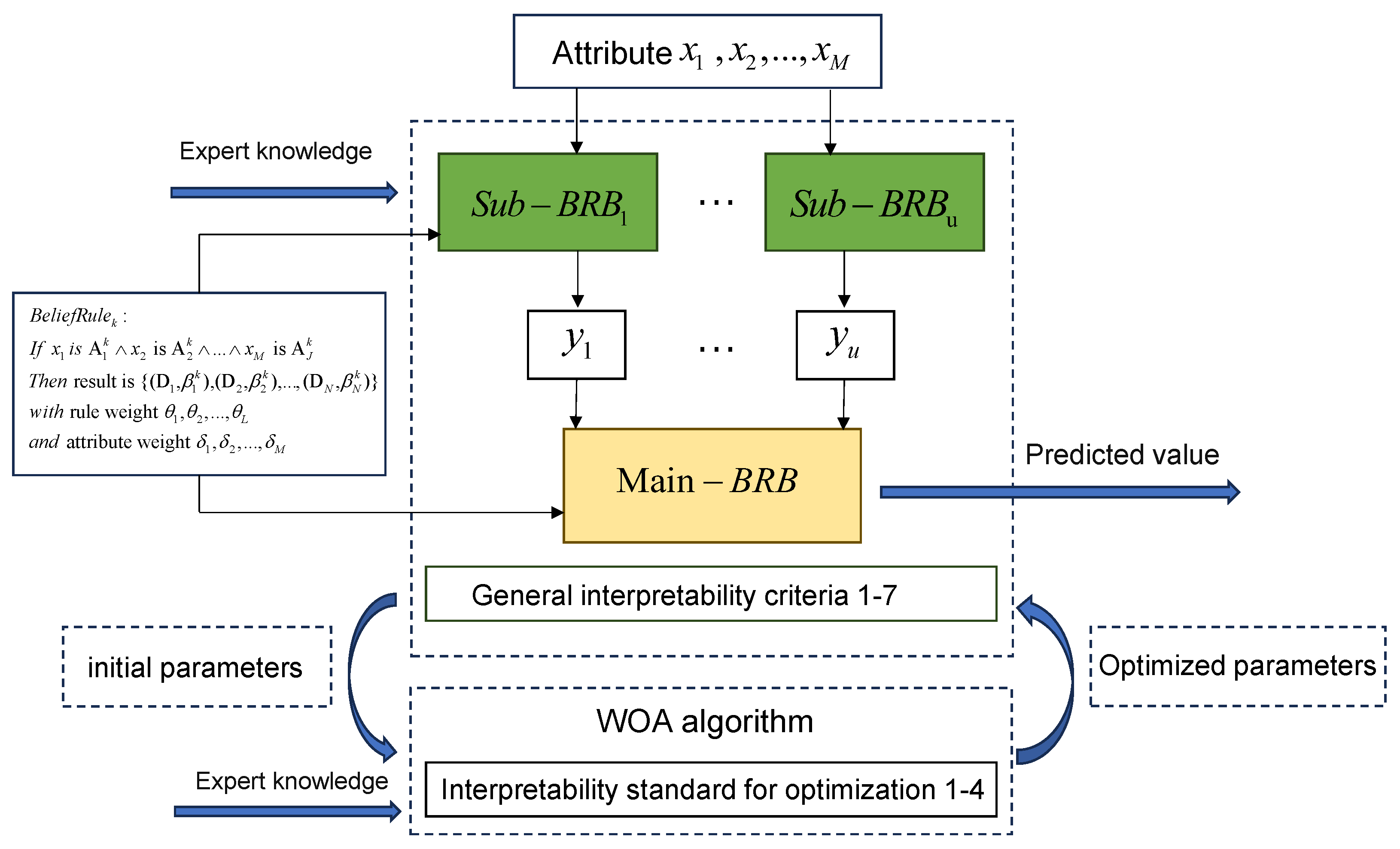
Predicting stock price trends is crucial for ensuring financial market stability, promoting rational resource allocation, and preventing systemic risks. Interpretable models can clearly present the logic and basis of stock price prediction, enabling investors and decision-makers to understand the model’s prediction process and thereby increasing their trust in the model’s prediction results. Therefore, to simultaneously ensure the interpretability and accuracy of the model, a new method based on hierarchical Belief Rule Base with balanced accuracy and interpretability for stock price trend prediction is proposed under interpretability constraints. The core architecture of the HBRB-b model is a hierarchical design, which solves the problem of explosive combination rules in the traditional BRB model. This structure is crucial for practical applications as it reduces the complexity of the model to a level that is auditable and manageable for human experts—a prerequisite for trusting financial analysis. Firstly, the input attributes are processed through multiple sub-BRBs. Each sub-BRB contains belief rules initialized by expert knowledge to generate intermediate results. Subsequently, the main BRB integrates these results to output the predicted values. The system employs the Whale Optimization Algorithm (WOA) to optimize rules and weights, simultaneously satisfying both general interpretability criteria and optimization-specific interpretability standards, thereby achieving a reasoning process that is both highly accurate and transparent. Figure 1 illustrates the overall structure of the interpretable stock price trend prediction model based on the WOA and the hierarchical Belief Rule Base. Section 4.1 Defines the interpretability of the model. The structure of the stock price trend prediction model is defined in Section 4.2. The reasoning process of the model is detailed in Section 4.3, while the optimization process is outlined in Section 4.4. Section 4.5 provides a practical exercise example.

4.1. Definition of Interpretability

To address regarding the preservation of financially logical expert knowledge during optimization, we first establish a set of interpretability criteria. These constraints are not merely mathematical formalities; they are designed to ensure the model’s outputs remain credible and actionable for financial experts. The interpretability of predictive models is highly significant for the stock market. Interpretability helps improve market efficiency, optimize resource allocation, reduce information asymmetry, and enhance investors’ financial literacy, thereby promoting the healthy development of the market through its educational effect [34]. Although the BRB expert system initially had certain advantages in terms of interpretability, achieving global interpretability in the complex and dynamic environment of the stock market remained challenging. In light of this, building on the general criteria for BRB interpretability proposed by Cao et al. [11], this paper further proposes several interpretability standards for the optimization process of stock price trend prediction models. These standards aim to enhance the overall transparency and credibility of the models in the stock market.

4.1.1. The Structural Interpretability of the Prediction Model

Criterion 1: The input reference values and their matching intervals can flexibly expand their semantics.

Standardizing the matching degree can generate intuitive and understandable semantic expressions. Meanwhile, the matching normalization operation ensures that within the domain X, each reference value has at least one data point with a matching score of 1, and all matching scores are strictly controlled within the interval from 0 to 1. The system should have clear semantics, which can be specifically described by Equation (4).

$$\begin{array}{c}\hfill \forall 1\le V\le Z,\exists x_p\in X,a_V\left(x_p\right)=1.\\ \hfill \forall 1\le V\le Z,x\in X,0\le a_V\left(x\right)\le 1.\end{array}$$

(4)

where Z represents the number of reference values of the predicted attribute, $x_p$ represents a fixed value in the domain, $a_V\left(x\right)$ represents the matching degree of the $V_{\mathrm{th}}$ reference value, and X represents the entire feasible domain.

Criterion 2: The system should have a complete rule base.

The integrity of the rule base requires that the rules in the BRB cover all possible operating states of the system. Specifically, the antecedents of the rules should encompass every possible value of all attributes, as described in Equation (5). This ensures that any input can match at least one reference value, thereby triggering at least one rule.

$$\forall x\in X\left\{\begin{array}{cc}\exists 1\le V\le Z,\hfill & a_V\left(x\right)>0\hfill \\ \exists 1\le l\le L\hfill & 0<w_l\le 1\hfill \end{array}\right.$$

(5)

where L represents the number of rules and $w_l$ indicates the activation weight of the $l_{\mathrm{th}}$ rule.

Criterion 3: Simplicity of the rule base.

In the stock price trend prediction model, rules are designed to capture expert knowledge in the form of IF-THEN statements. However, an excessive number of prerequisite attributes for the rules can overwhelm experts’ ability to handle real-world situations. Therefore, the number of attributes and reference values in the BRB should be kept moderate to ensure a reasonable number of rules and better readability of the BRB.

Criterion 4: Consistency of rules.

Ensuring the consistency of rules can effectively eliminate ambiguity in the final results. During the modeling process, conflicting rules are unacceptable because they are difficult to interpret. Reasonably extracting expert knowledge, transforming it into rules, and then constructing a rule base is a highly effective approach.

Criterion 5: System parameters should have physical significance.

When constructing a stock price trend prediction model, it is essential to ensure that reasonable causal relationships can be derived. Therefore, every parameter in the model evaluation process should have clear practical significance. In the belief rule model, the parameters involved include the following:

(1)

Rule weights: These are used to measure the importance of different rules.

(2)

Attribute weights: These reflect the importance of the indicators.

(3)

Activation weights: These describe the extent to which the rules are activated.

(4)

Belief level: Describes the degree to which the rule matches the state of the stock price trend.

All these parameters are normalized within the range of 0 to 1, which can be described by Equation (6).

$$\{\delta ,\theta ,\beta ,\omega \}\in [0,1]$$

(6)

Criterion 6: Transparent reasoning engine.

The belief rules within the Belief Rule Base (BRB) form the foundation of the reasoning process. Efficiently applying these rules to generate predictions is crucial. The Evidence Reasoning (ER) algorithm, with its rigorous mathematical derivation, achieves accurate results through probabilistic synthesis. Utilizing the ER algorithm as the reasoning engine endows the BRB with a clear and transparent reasoning process.

Criterion 7: Reasonable information transformation.

To ensure the reliability of the reasoning process, it is essential to conduct reasonable transformations that maintain the coherence and consistency of information. During the reasoning process, the system should preserve the integrity of the initial information as much as possible while achieving efficient information transformation within the belief structure. The ER method, based on rules and utility, is an exemplary algorithm. It possesses equivalent and reasonable information transformation capabilities within the belief structure, effectively supporting the reasoning process.

4.1.2. The Optimization Interpretability of the Prediction Model

To address the issue of preserving expert knowledge in financial logic during the optimization process, a set of Interpretability optimization criterias was first established. These constraints are not merely mathematical formalities; they are designed to ensure that the model’s outputs remain credible and actionable for financial experts.

The interpretability of the Belief Rule Base (BRB) is primarily reflected in its ability to integrate expert knowledge into the model [35]. However, the initial parameters determined by experts are often subjective, which to some extent limits the accuracy of the model’s prediction of stock price trends. Therefore, BRB needs to be trained and optimized using historical observation data. During this optimization process, however, BRB may face the challenge of maintaining interpretability effectively. To address this, the following Standards are proposed in this paper to ensure the interpretability of BRB during optimization.

Standard 1: Effective utilization of expert knowledge.

Expert knowledge serves as a foundational component of model interpretability. The optimization process should fully integrate expert judgment to achieve precise local search. Therefore, when constructing the initial population, incorporating expert knowledge and optimizing it in conjunction with the Euclidean distance can effectively enhance the accuracy within the local search domain. This approach can be described by Equations (7) and (8).

$$m^{\left(g\right)}=\left\{\begin{array}{cc}EK\hfill & \mathrm{if}g=1\hfill \\ m^{\left(g\right)}\hfill & \mathrm{if}g\ne 1\hfill \end{array}\right.$$

(7)

where $m^{\left(g\right)}$ is the population in the $g_{\mathrm{th}}$ generation; $EK$ represents expert knowledge. Interpretability Criterion 8 ensures the initial interpretability of the model by converting expert knowledge into parameters.

$$\rho (h_n,h_n^{\prime })=\sqrt{{(h_1-h_1^{\prime })}^2+{(h_2-h_2^{\prime })}^2+\dots +{(h_n-h_n^{\prime })}^2}=\sqrt{\sum _{i=1}^n{(h_i-h_i^{\prime })}^2}$$

(8)

where $h_i$ represents expert knowledge, $h_i^{\prime }$ is the optimized parameter, and $\rho (h_n,h_n^{\prime })$ is the Euclidean distance between the expert knowledge and the optimized parameter.

Standard 2: The optimized rules should not deviate significantly from the expert’s judgment.

The parameters of the BRB model directly reflect the underlying physical or statistical laws. Unlike the opaque nature of black-box models, the BRB model is more easily understood and accepted by users. Therefore, it is essential to ensure that these key parameters are fully and appropriately applied within the model. To address this, the model introduces parameter constraints, as shown in Equation (9).

$$\begin{array}{cc}\hfill p_{lp}\le p\le p_{up}:& \left\{{\theta }_{l{p}_i}\le {\theta }_i\le {\theta }_{u{p}_i}i\in \{1,2,\dots ,L\},\right.\hfill \\ \hfill & {\delta }_{l{p}_m}\le {\delta }_m\le {\delta }_{u{p}_m}m\in \{1,2,\dots ,M\},\hfill \\ \hfill & \left.{\beta }_{l{p}_n}\le {\beta }_n\le {\beta }_{u{p}_n}n\in \{1,2,\dots ,N\}\right\}\hfill \end{array}$$

(9)

where $p_{lp}$ is the minimum value of the parameter, $p_{up}$ is the maximum value of the parameter, ${\theta }_l$ represents the rule weight of the $l_{\mathrm{th}}$ belief rule, ${\delta }_m$ represent the attribute weight of the $m_{\mathrm{th}}$ prediction indicator, and ${\beta }_n$ indicates the belief level corresponding to each result.

Standard 3: Unactivated rules do not participate in optimization.

When the $l_{\mathrm{th}}$ rule is activated, the related activation parameters $\{\delta ,\theta ,\beta \}$ will participate in the optimization process, while the unactivated parameters should maintain their initial expert knowledge settings. Therefore, identifying and distinguishing invalid rules is crucial for the effective operation of the model. As shown in Formula (10).

$${\Omega }_m^{g+1}=BR{B}_{\mathrm{initial}}({\beta }_k,{\theta }_k)$$

(10)

where ${\Omega }_m^{g+1}$ represents the $m_{\mathrm{th}}$ parameter vector and $BR{B}_{\mathrm{initial}}({\beta }_k,{\theta }_k)$ represents the relevant parameters of the $k_{\mathrm{th}}$ rule in the initial rule base. The substitution operation replaces only the parameters corresponding to valid rules and forms a new solution vector.

Standard 4: Reasonable belief distribution.

Belief rules integrate expert knowledge into the model in the form of parameters, enabling the model to generate logically sound and persuasive prediction results. However, an excessive focus on accuracy while neglecting interpretability can easily lead to a proliferation of incorrect rules that do not align with reality. To address this issue, the constraints on the belief distribution of each rule are presented in Equation (11).

$$\begin{array}{cc}\hfill U_{\beta }:& \left\{\left\{{\beta }_1\le {\beta }_2\le \dots \le {\beta }_n\right\}\right.\hfill \\ \hfill & \mathrm{or}\left\{{\beta }_1\ge {\beta }_2\ge \dots \ge {\beta }_n\right\}\hfill \\ \hfill & \mathrm{or}\left\{{\beta }_1\le \dots \le max({\beta }_1,{\beta }_2,\dots ,{\beta }_n)\ge \dots \ge {\beta }_n\right\}\hfill \end{array}$$

(11)

where $U_{\beta }$ represents the constraint on the belief distribution. Suppose the prediction of the stock price trend is (very low, 0.6), (low, 0.2), (medium, 0.1), (high, 0.1). However, the optimized belief distribution might be (very low, 0.6), (low, 0), (medium, 0), (high, 0.4). If the belief distribution is concave, it means that the prediction results are in both low and high states simultaneously, which is unreasonable in the real world. The reasonable shape of the belief distribution should be monotonic or convex. As shown in Figure 2.

4.2. Construction of an Interpretable Stock Price Trend Prediction Model Based on WOA and Hierarchical Belief Rule Base

In the HBRB-b model, the prediction process initiates from the underlying sub-BRBs, which aggregate the attributes of their inputs. The output of each sub-BRB then becomes the input for the subsequent higher-level BRB. This hierarchical transmission continues layer by layer until it reaches the top-level BRB. Ultimately, the inference is completed at the top-level BRB to yield the final prediction result. Each BRB in this process follows the form of Equation (12).

$$\begin{array}{cc}\hfill & {\mathit{BeliefRule}}_k:\hfill \\ \hfill & \mathit{If}{x}_1\mathit{is}{A}_1^k\wedge x_2\mathit{is}{A}_2^k\wedge \dots \wedge x_M\mathit{is}{A}_J^k\hfill \\ \hfill & \mathit{Then}\mathit{result}\mathit{is}\{(D_1,{\beta }_1^k),(D_2,{\beta }_2^k),\dots ,(D_N,{\beta }_N^k)\}\hfill \\ \hfill & \mathit{with}\mathit{rule}\mathit{weight}{\theta }_1,{\theta }_2,\dots ,{\theta }_L\hfill \\ \hfill & \mathit{and}\mathit{attribute}\mathit{weight}{\delta }_1,{\delta }_2,\dots ,{\delta }_M\hfill \\ \hfill & \mathrm{in}{p}_1,p_2,\dots ,p_{m}and{c}_1,c_2,\dots ,c_h\hfill \end{array}$$

(12)

where $x_1,x_2,\dots ,x_M$ are the leading attributes of stock price trend prediction, $A_1^k,A_2^k,\dots ,A_J^k$ represent the reference values for each attribute, ${\theta }_1,{\theta }_2,\dots ,{\theta }_L$ represent the weights of each rule, ${\delta }_1,{\delta }_2,\dots ,{\delta }_M$ represent the weights of each attribute, $D_1,D_2,\dots ,D_N$ represent the prediction results, ${\beta }_1^k,{\beta }_2^k,\dots ,{\beta }_N^k$ represent the corresponding belief levels, L indicates the number of rules, M indicates the number of prior attributes, and N indicates the quantity of the results.

4.3. Evidence Reasoning Method

The HBRB-b model ultimately derives the prediction result through a bottom-up, layer-by-layer reasoning process. In accordance with the interpretability criteria introduced in Section 4.1, the reasoning process of each BRB can be described as follows.

Initially, the matching degree between the input data and the reference value is computed based on Equation (13).

$$\begin{array}{cc}\hfill S\left(x_i\right)& =\left\{\left(A_{i,j}^k{\alpha }_{i,j}^k\right)\mid i=1,\dots ,T_k,j=1,\dots ,J\right\}\hfill \\ \hfill {\alpha }_{i,j}^k& =\left\{\begin{array}{cc}{\displaystyle \frac{A_{i,j+1}^k-x_i}{A_{i,j+1}^k-A_{i,j}^k}}\hfill & ,j=k\left(A_{i,j}^k\le x_i\le A_{i,j+1}^k\right)\hfill \\ {\displaystyle \frac{x_i-A_{i,j}^k}{A_{i,j+1}^k-A_{i,j}^k}}\hfill & ,j=k+1\hfill \\ 0\hfill & ,j=1,\dots ,J(j\ne k,k+1)\hfill \end{array}\right.\hfill \end{array}$$

(13)

where $S\left(x_i\right)$ represents the information transformation process of the input data $x_i$, ${\alpha }_{i,j}^k$ represents the matching degree of the $j_{\mathrm{th}}$ reference value belonging to the $i_{\mathrm{th}}$ attribute, J indicates the number of reference values, and $A_{i,j}^k$ and $A_{i,j+1}^k$ indicate the number of reference values.

After obtaining the matching degree information for the data corresponding to each rule, the activation weights are subsequently calculated. The calculation is illustrated in Equation (14):

$$\begin{array}{c}\hfill {\omega }_k={\displaystyle \frac{{\theta }_k{\displaystyle \prod _{i=1}^{T_k}}{\left(a_{i,j}^k\right)}^{{\delta }_i}}{{\displaystyle \sum _{l=1}^L}{\theta }_l{\displaystyle \prod _{i=1}^{T_k}}{\left(a_{i,j}^l\right)}^{{\delta }_i}}},\overline{{\delta }_i}={\displaystyle \frac{{\delta }_i}{max\left\{{\delta }_i\right\}}}\end{array}$$

(14)

where ${\omega }_k$ represents the activation weight of rule $k_{\mathrm{th}}$ and $\overline{{\delta }_i}$ represents the relative weight of the attribute.

Subsequently, reasoning is conducted based on the activated rules, and the ER algorithm is employed to calculate the belief level of the results. The specific reasoning process can be referred to in Equations (15) and (16).

$${\beta }_n={\displaystyle \frac{\mu \left[{\prod }_{k=1}^L\left({\omega }_k{\beta }_{n,k}+1-{\omega }_k{\sum }_{j=1}^N{\beta }_{j,k}\right)-{\prod }_{k=1}^L\left(1-{\omega }_k{\sum }_{j=1}^N{\beta }_{j,k}\right)\right]}{1-\mu \left[{\prod }_{k=1}^L\left(1-{\omega }_k\right)\right]}}$$

(15)

$$\mu ={\left[\sum _{n=1}^N\prod _{k=1}^L\left({\omega }_k{\beta }_{n,k}+1-{\omega }_k\sum _{j=1}^N{\beta }_{j,k}\right)-(N-1)\prod _{k=1}^L\left(1-{\omega }_k\sum _{j=1}^N{\beta }_{j,k}\right)\right]}^{-1}$$

(16)

The final belief distribution can be expressed by Equation (17):

$$S\left(x\right)=\left\{\left(D_n,{\beta }_n\right)\mid n=1,2,\dots ,N\right\}$$

(17)

where $S\left(x\right)$ represents the belief distribution obtained based on a set of attribute data. Ultimately, the reasoning result of the model is calculated through Equation (18).

$$u\left(S\left(x\right)\right)=\sum _{n=1}^{N}u\left(D_n\right){\beta }_n$$

(18)

where $u\left(S\right(x\left)\right)$ represents the final output result of the model, $u\left(D_n\right)$ represents the utility value of the result level.

4.4. The Optimization Process of the Model

To address the issue of how constrained optimization algorithms can strike a balance between interpretability and accuracy, an improved Whale Optimization Algorithm (WOA) is proposed to optimize the BRB parameters. However, the key point is to directly integrate the interpretability constraints in Section 4.1 into the optimization process. This ensures that the pursuit of predictive accuracy does not compromise interpretability, and that the model’s reasoning remains explainable and intuitive to portfolio managers. The standard WOA operation is detailed in Appendix A. It was selected after carefully considering the existing optimization approaches, including the Projection Covariance Matrix Adaptive Evolution Strategy (P-CMA-ES) and Particle Swarm Optimization (PSO). As a nature-inspired metaheuristic algorithm, WOA demonstrates four distinct advantages that make it particularly suitable for BRB optimization: (1) Parameter efficiency: Requiring fewer tuning parameters than comparable algorithms while maintaining implementation simplicity [36,37]. (2) Computational efficiency: Exhibiting faster convergence rates in empirical testing [38]. (3) Robust search capability: Demonstrating superior ability to escape local optima through its unique spiral updating mechanism [39]. (4) Domain adaptability: Proven effective across diverse optimization problem domains [40]. These characteristics collectively position WOA as an optimal choice for enhancing BRB performance while maintaining the model’s interpretability, a crucial requirement for financial prediction systems.

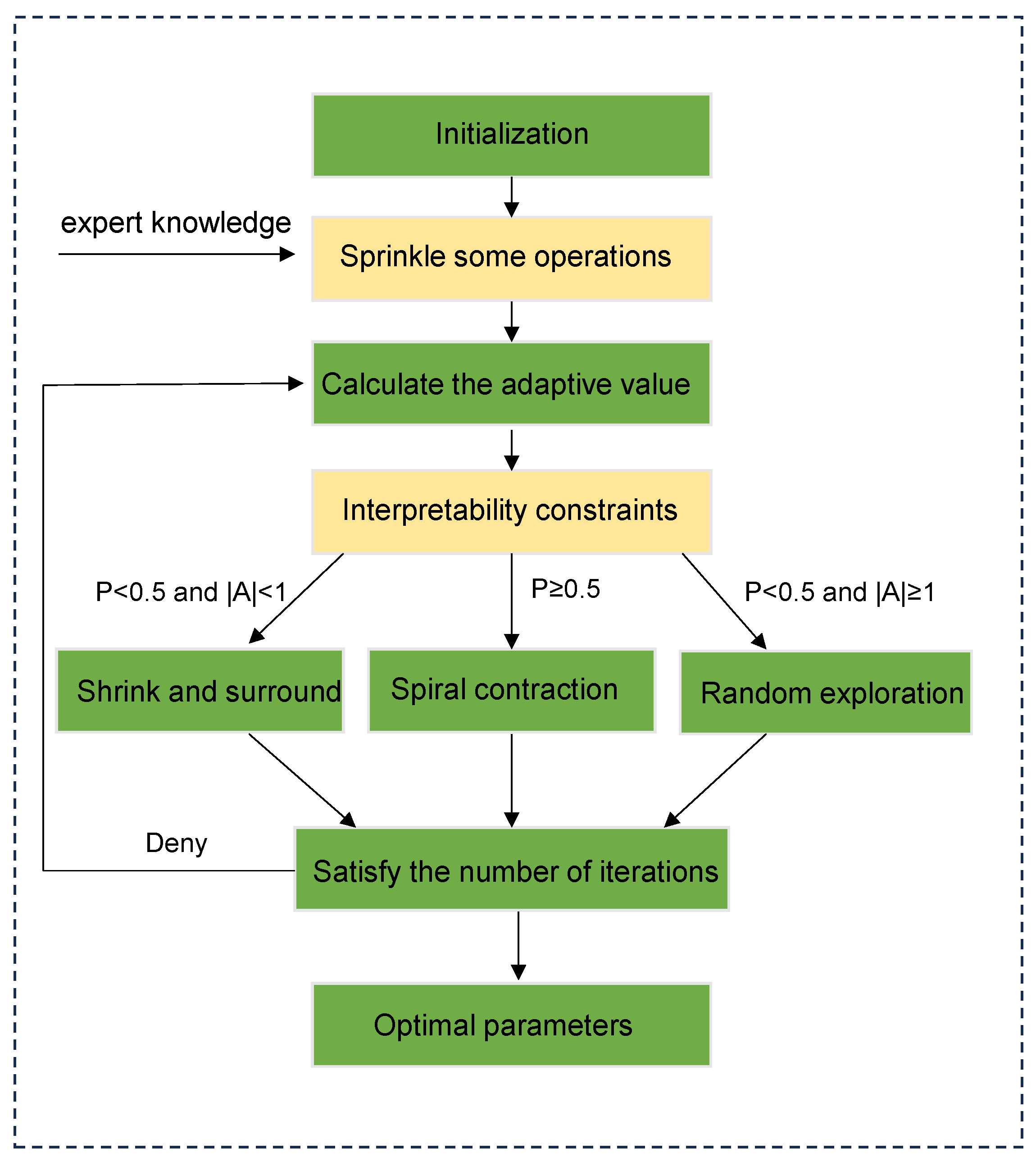
To ensure the interpretability of the model optimization process, this paper adds interpretability constraints on the basis of the original WOA. Figure 3 shows the flowchart of the WOA with interpretability constraints, and its specific optimization steps are as follows.

Step 1: Initialization: Define the number of iterations as the population size of whales, and the size of the search space as the dimension.

Step 2: Scattered point operation: In the model based on HBRB-b, its interpretability partly stems from expert knowledge formed based on long-term practice. However, the traditional WOA adopts the method of randomly scattering points, and its utilization efficiency of expert knowledge is relatively low. To solve this problem, a new dotting strategy was designed based on the optimized version of the HBRB-b model. This strategy first constructs a solution space with expert knowledge as the core, and then scatters points in a specific area around the expert knowledge, thereby improving the utilization of expert knowledge and enhancing the interpretability of the model.

Points are randomly scattered based on expert knowledge. The position vector of each whale is represented by $\alpha$, which represents a set of parameters in the reasoning process. Among these parameters, the position of the i-th whale can be expressed by Formula (19):

$${\alpha }_i=F_k+(\mathrm{rand}(\alpha ,v)-0.5)\times 2$$

(19)

where $F_k$ denotes the belief level determined by expert knowledge, and $\mathrm{rand}(\alpha ,v)$ generates an o×v random matrix with elements uniformly distributed between 0 and 1.

Step 3: Calculate the adaptive value: Take the mean square error (MSE) as the objective function.

$$\left\{\begin{array}{c}min\{\alpha =\{\theta ,\delta ,\beta \left\}\right\}\hfill \\ \mathrm{s}.\mathrm{t}.0\le \theta \le 1,0\le \delta \le 1,0\le \beta \le 1\hfill \end{array}\right.$$

(20)

where $\alpha =\{\theta ,\delta ,\beta \}$ is the error between the true value and the model’s predicted result.

Step 4: Constraint operation: The inherent randomness of the traditional Whale Optimization Algorithm (WOA) fails to meet the interpretability requirements for stock price trend prediction. To address this, incorporating constraint conditions ensures that the model remains interpretable throughout the optimization process.

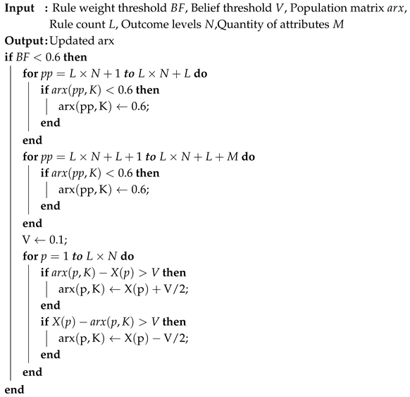
Constraint 1: While expert knowledge may not be able to precisely determine specific belief values for each rule, the belief levels defined by expert knowledge can still meet the overall requirements of the system. During the model optimization process, to ensure that the model’s interpretability is not compromised, the adjustments to rule belief must align with expert knowledge and avoid contradicting it. Therefore, it is necessary to establish a reasonable range for the belief level of each rule. This is specifically represented by Formula (9). The pseudo-code of the Algorithm 1 is as follows.

Algorithm 1: Constraint Enforcement for Weights and Beliefs

Constraint 2: The belief rule is a crucial aspect that reflects the interpretability of the HBRB-b model. However, the belief distribution generated by the current optimization process often exhibits significant inconsistencies with the actual stock price trends. To address this, the optimized belief distribution must be aligned with the actual stock price trends. This constraint is specifically formulated and represented by Equation (11). The pseudo-code of the Algorithm 2 is as follows.

Step 5: Population update. The population is updated according to the standard WOA mechanisms (detailed in Appendix A), which balance exploration and exploitation through their unique encircling and spiral movements.

The iterative process (Steps 3–5) continues until the maximum number of iterations is reached, yielding the optimized yet interpretable parameters.

Algorithm 2: Constraint Enforcement for Reasonable Belief Distribution

4.5. A Practical Walkthrough Example

To illustrate how the HBRB-b model functions in a realistic scenario, we present a detailed walkthrough using hypothetical but representative data. This example demonstrates the model’s hierarchical reasoning process and, most importantly, how its interpretable output can be utilized by a financial analyst for decision-making.

Consider an analyst who needs to assess the market trend for the next trading day. The normalized market data for the current day is as follows: the Open Price ($x_1$) is 0.55, the Close Price ($x_2$) is 0.48, the High Price ($x_3$) is 0.62, and the Low Price ($x_4$) is 0.45. These values represent a day on which the market opened at a moderate level, closed lower, and traded within a range.

The model begins processing by transforming these raw input values into matching degrees against the predefined linguistic reference values (e.g., Very Low, Low, Medium, High, Very High) using the transformation method described in Equation (13). For instance, the Close Price of 0.48 might be assessed as having a 60% match to “Low” and a 40% match to “Medium”, indicating a bearish closing sentiment.

Subsequently, each sub-BRB performs its dedicated analysis. Sub-BRB₁, which processes the Open and Close prices, synthesizes its inputs and, through the Evidence Reasoning algorithm, produces an intermediate result. Let us assume its output is a belief distribution of $\left\{\right(Low,0.7),(Medium,0.3\left)\right\}$. This signifies that the combined signal from the opening and closing dynamics is most strongly indicative of a “Low” trend outcome.

Simultaneously, sub-BRB₂, tasked with analyzing the High and Low prices to gauge volatility, produces its own intermediate result. Assume its output is $\left\{\right(Medium,0.5),(High,0.5\left)\right\}$. This indicates a state of high market volatility lacking a clear directional signal from the day’s trading range.

These two intermediate results, $y_1$ and $y_2$, then serve as the inputs to the main, integrating BRB. This top-level model evaluates which of its high-level rules are activated by these inputs. A rule such as ‘IF sub-BRB₁ Output is Low AND sub-BRB₂ Output is Medium THEN…’ would be strongly triggered in this scenario.

The Main-BRB then synthesizes all activated rules using the Evidence Reasoning algorithm (Equations (15)–(18)) to produce the final, comprehensive belief distribution. The output might be $S\left(\mathrm{Next}\mathrm{Day}\right)=\left\{\right(\mathrm{Down},0.60),(\mathrm{Neutral},0.30),(\mathrm{Up},0.10\left)\right\}$.

This final output provides the analyst with a nuanced and immediately actionable forecast. The highest confidence (60%) is assigned to a downward market movement, which would suggest considering defensive actions such as hedging or reducing exposure. Crucially, the significant combined belief (40%) in non-downward outcomes (Neutral or Up) clearly quantifies the underlying uncertainty, cautioning against an overly aggressive defensive strategy and prompting further investigation into other market factors.

Furthermore, the analyst can audit the model’s reasoning by inspecting which specific rules were activated with high weight. Discovering that a rule linking “Low closing price” with “High volatility” was a primary contributor validates the model’s logic against established technical analysis principles, thereby building trust and confidence in the final prediction. This walkthrough exemplifies the model’s core strength: generating not merely a prediction but a reasoned, transparent, and actionable assessment for financial decision-making under uncertainty.

5. Case Study

In this section, a stock price trend dataset is used as an example to test the validity of the prediction model based on HBRB-b. In Section 5.1, the introduction of the dataset was carried out. In Section 5.2, a stock price trend prediction model based on HBRB-b was developed. In Section 5.3, the interpretability of the model based on HBRB-b was verified. In Section 5.4, cross-validation was carried out. In Section 5.5, a comparative experiment was conducted.

5.1. Introduction to the Dataset

This research used the dataset found in https://www.kaggle.com/datasets/gelasiusgalvindy/stock-indices-around-the-world, accessed on 11 September 2025. The dataset, collected from Yahoo Finance, consists of daily stock trading indicators for the period from 17 July 2017 to 2 July 2022. The dataset used in this research includes daily price data of multiple major global stock indices, specifically the following: the Dow Jones Industrial Average (DJI), the S&P 500 Index (SPX), the Nasdaq Composite Index (IXIC), the CBOE Volatility Index (VIX), the FTSE 100 Index (FTSE), the Paris CAC40 Index (FCHI), the European STOXX 600 Index (STOXX), the Dutch AEX Index, and the Spanish I The BEX Index, the Russian MOEX Index, the Turkish BIST Index, the Hong Kong Hang Seng Index (HSI), the Shanghai Composite Index (SSE), etc. Stock data changes exhibit nonlinearity, non-stationarity, and high complexity. The constructed stock price prediction system should not only be able to effectively handle uncertain information, but must also have interpretability to ensure its prediction results have high credibility. The detailed descriptions of the selected indicators are shown in

Table 1. Input and output variables used for stock price trend prediction.

Variable	Name	Description	Rationale for Selection
$x_1$	Daily Closing Price	The final price at which a stock is traded on a given day.	The most fundamental indicator, representing the market’s consensus on the stock’s value at the end of the day.
$x_2$	Daily Closing Price	The first transaction price of a certain financial product at the beginning of a trading day.	It can reflect the initial supply and demand relationship in the market and investors’ expectations, providing a basic reference for subsequent price changes.
$x_3$	Daily High Price	The highest price reached during the day.	Represents the maximum upward pressure and helps gauge resistance levels and market optimism.
$x_4$	Daily Low Price	The lowest price reached during the day.	Represents the maximum downward pressure and helps gauge support levels and market pessimism.
y	Next Day’s Closing Price	The closing price of the following trading day.	The target variable for prediction model.

. The dataset includes 1280 index data points, among which the first 60% are used as training data and the last 40% as test data.

To prepare the data for modeling, the following preprocessing steps were applied:

Handling Missing Values: The dataset was first inspected for missing or anomalous values. Any days with missing entries were removed from the analysis to ensure data integrity. This resulted in a clean dataset of 1280 consecutive trading days.

Normalization: Due to the varying units and numerical ranges of different features, gradient updates during model training can become slower. Therefore, the data were standardized and scaled to the interval (0, 1). The standardized formula is shown in Formula (21). Figure 4 presents the relationship between the four normalized attributes and the stock price of the next day.

$$\tilde{x}={\displaystyle \frac{x-x_{min}}{x_{max}-x_{min}}}$$

(21)

5.2. Construction and Optimization of Stock Price Trend Prediction Model Based on HBRB-b

The proposed HBRB-b model for stock price prediction is configured as follows:

Input Attributes: Four input features are selected: $x_1$ (Normalized Daily Opening Price), $x_2$ (Normalized Daily Closing Price), $x_3$ (Normalized High Price), and $x_4$ (Normalized Low Price). These features are divided into two groups.

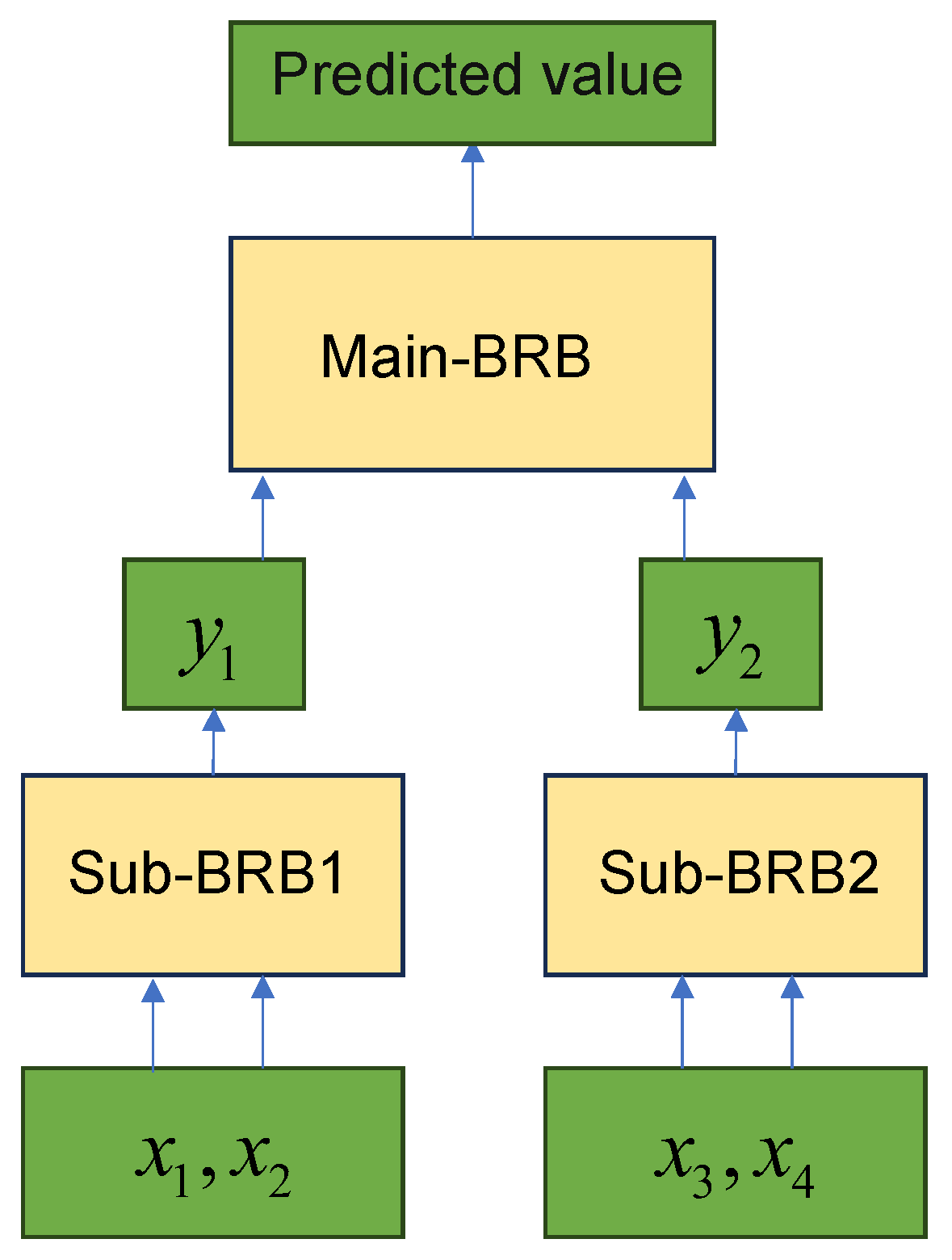
Sub-BRB1: Takes $x_1$ and $x_2$ as inputs and produces an intermediate result $y_1$. Sub-BRB2: Takes $x_3$ and $x_4$ as inputs and produces an intermediate result $y_2$. The Main-BRB integrates these results to output the final prediction of the next day’s normalized closing price. The use of daily data enables the model to capture short-term market trends and volatilities, which are essential for daily trading decisions.

Rule Base Size: Each sub-BRB contains 25 rules (5 reference points for input 1 and 5 reference points for input 2). The Main-BRB also contains 25 rules. This structure effectively reduces the total number of rules from $5^4$ = 625 (in a traditional BRB) to 25 + 25 + 25 = 75, demonstrating its advantage in combating combinatorial explosion.

Table 2. Comparison of rule numbers between traditional BRB and HBRB-b.

Number of Input	Traditional BRB	HBRB-b
Attributes
4	$5^4=625$	$2\times 5^2+5^2=75$
6	$5^6=15,625$	$2\times 5^3+5^2=275$
8	$5^8=390,625$	$2\times 5^4+5^2=1275$
10	$5^{10}=9,765,625$	$2\times 5^5+5^2=6375$

compares the complexity of different numbers of attributes for the traditional BRB model and the HBRB-b model.

The HBRB-b model fundamentally improves the scalability of the model through its hierarchical structure. As shown in the comparative analysis, the number of rules in traditional BRB grows exponentially with the input features, leading to a combination explosion when the number of features is large. HBRB-b successfully reduces the complexity to a polynomial level, generating only hundreds or even thousands of rules under the same conditions and achieving a reduction of several orders of magnitude. Thereby significantly enhancing the model’s ability to handle high-dimensional problems.

Output: The Main-BRB outputs the predicted trend as a belief distribution over the linguistic terms VL, L, M, H, and VH, which is then defuzzified into a numerical value using utility scores.

To construct the initial model based on HBRB-b, belief rules need to be formulated. According to the evaluation of experts, five semantic levels—“Very Low” (VL), “Low” (L), “Medium” (M), “High” (H), and “Very High” (VH)—were selected to represent the state of the system, as shown in Formula (22).

$$\begin{array}{cc}\hfill & \mathit{BeliefRule}:\hfill \\ \hfill & \mathit{If}{y}_1\mathit{is}{A}_1\wedge y_2\mathit{is}{A}_2\hfill \\ \hfill & \mathit{Then}\mathit{result}\mathit{is}\{(V{L}_1,{\beta }_1),(L_2,{\beta }_2),(M_3,{\beta }_3),(H_4,{\beta }_4),(V{H}_5,{\beta }_5)\}\hfill \\ \hfill & \mathit{with}\mathit{rule}\mathit{weight}{\theta }_1,{\theta }_2,\dots ,{\theta }_{25}\hfill \\ \hfill & \mathit{and}\mathit{attribute}\mathit{weight}{\delta }_1,{\delta }_2\hfill \\ \hfill & \mathrm{in}{p}_1,p_2,\dots ,p_{7}and{c}_1,c_2,\dots ,c_4\hfill \end{array}$$

(22)

This model consists of two sub-rule bases, named sub-BRB1 and sub-BRB2, respectively. Each sub-rule base is responsible for integrating two sets of attributes and generating outputs y1 and y2. The BRB at the top, called the Main-BRB, integrates the outputs from the sub-BRBs to infer the final prediction. The structure of the model is shown in Figure 5.

Based on expert knowledge and a detailed analysis of the indicator data, five reference values were defined for each indicator. The sum of the matching degrees of these reference values with the current input index data is limited within the range of 0 to 1.

Table 3. Reference values and semantic labels for input and output variables in the HBRB-b model.

BRB	Input	Reference Point	Reference Value	Attribute Weight
Sub-	$x_1$	(VL,L,M,H,VH)	(0,0,2,0.5,0.7,1)	1
BRB1	$x_2$	(VL,L,M,H,VH)	(0,0.2,0.5,0.7,1)	1
Sub-	$x_3$	(VL,L,M,H,VH)	(0,0.2,0.5,0.7,1)	1
BRB2	$x_4$	(VL,L,M,H,VH)	(0,0.2,0.5,0.7,1)	1
Main-	$y_1$	(VL,L,M,H,VH)	(0,0.2,0.5,0.7,1)	1
BRB	$y_2$	(VL,L,M,H,VH)	(0,0.2,0.5,0.7,1)	1
Output	-	(VL,L,M,H,VH)	(0,0.2,0.5,0.7,1)	-

shows the reference points and their reference values of the input indicators and output results. Furthermore, the stock price prediction model based on HBRB-b is constructed by leveraging professional experience in the field, and Appendix B.1 lists the initial rule configuration of this model.

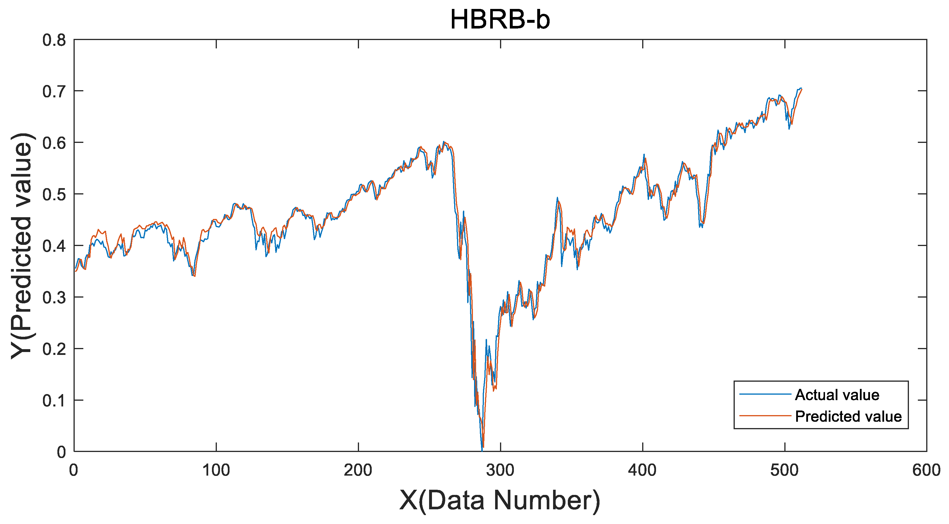
The initial model was optimized using the improved WOA. Considering that the results obtained by sub-BRB often lack comprehensiveness, therefore, in the optimization process, the global optimization method was adopted to avoid falling into local optimum. The initial parameters of the WOA are set as follows: a population size of 20,400 iterations, and an optimization dimension of 152. The stock price trend dataset used contains 1280 sets of data, among which 768 sets are used for training and the remaining 512 sets are used for testing. The prediction results of the optimized model are shown in Figure 6, and the mean square error between the predicted value and the actual value is 4.5392 × 10⁻⁴. This indicates that the HBRB-b model fits the data well and produces highly accurate predictions. The optimized rule parameters are detailed in Appendix B.2.

5.3. Interpretability Analysis

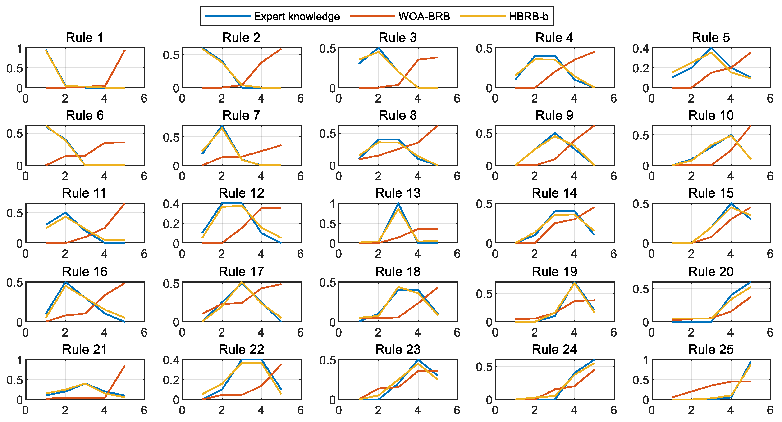
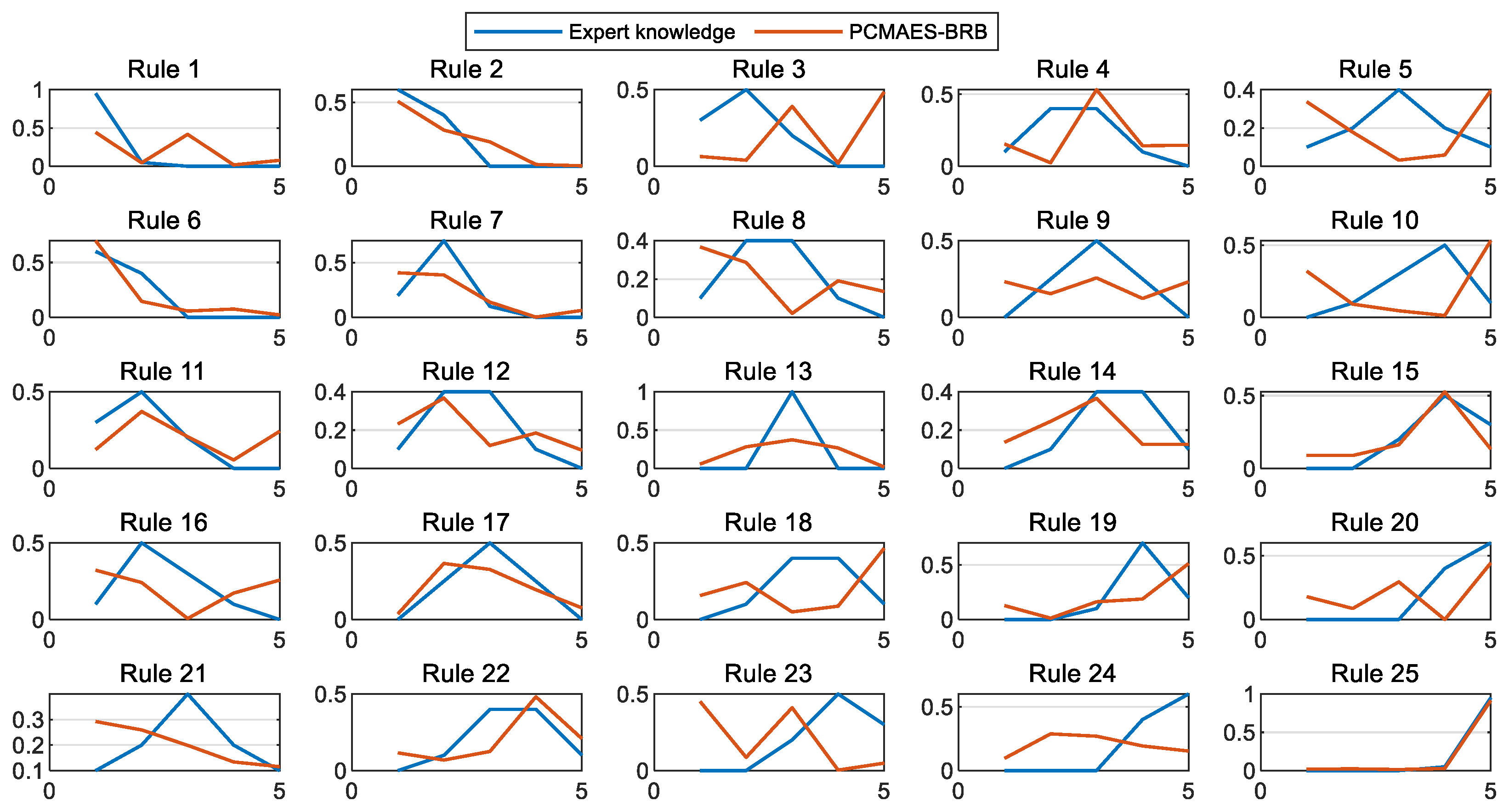
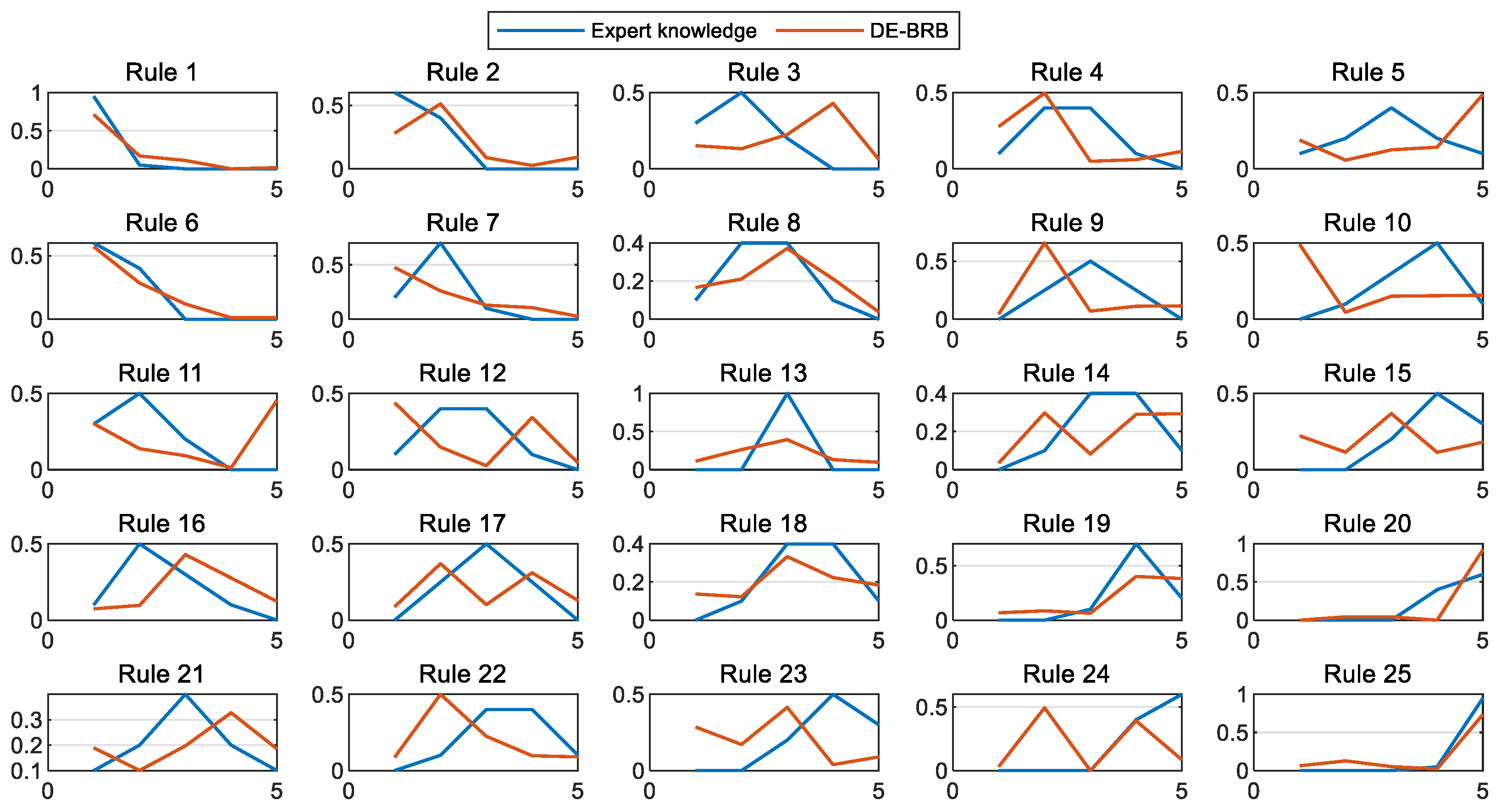
To evaluate the interpretability of the models, this section compares the PCMAES-BRB, DE-BRB, WOA-BRB, and HBRB-b models, with a focus on analyzing the belief distribution of the initial rules and the optimized rules of these models. As shown in Figure 7, Figure 8 and Figure 9, the optimized belief distribution in the HBRB-b model remains consistent with expert knowledge. This demonstrates that the model’s interpretability is effectively maintained and that the optimized rules retain high credibility. In contrast, the other three models deviated significantly from the initial expert judgments during optimization, substantially weakening their interpretability.

Derived from the Pythagorean theorem, the Euclidean distance is a fundamental metric for calculating the straight-line distance between points in a multidimensional space. It is computed by taking the square root of the sum of squared differences across each dimension and exhibits key characteristics such as intuitiveness, symmetry, non-negativity, and adherence to the triangle inequality. In machine learning applications, this distance metric plays a crucial role in measuring data point similarity and determining proximity relationships. The interpretability of the HBRB-b model stems from its foundation in expert knowledge, by which financial analysts and investment practitioners systematically transform accumulated experience into belief rules. These rules abstract factors influencing stock prices and potential market behaviors, formalizing expert insights into rule parameters with explicit practical significance. By ensuring the optimized rules and parameters remain consistent with expert judgments, the HBRB-b model maintains its interpretability in stock price prediction tasks. This study selects Euclidean distance as the core metric for evaluating model interpretability, with its specific calculation formula presented as Equation (8), and the comparative results across different models shown in

Table 4. Euclidean distance of different models.

Model	PCMAES-BRB	DE-BRB	WOA-BRB	HBRB-b
Euclidean distance	1.5078	1.9756	2.7372	0.3141

demonstrate that the HBRB-b model achieves superior performance by effectively minimizing the deviation from expert knowledge while preserving prediction accuracy, thereby establishing an optimal balance between computational optimization and interpretability maintenance that is particularly valuable for financial decision-making scenarios requiring both transparency and reliability. The adoption of Euclidean distance as an interpretability evaluation index is well justified given its mathematical properties that enable effective verification of the consistency between data-driven optimizations and domain expertise.

During the optimization process, the HBRB-b model is centered on expert knowledge. Through precise parameter adjustment and rule optimization, the Euclidean distance between the optimized rules and expert knowledge is minimized. This minimization is not only reflected numerically, but also means that the optimized rules are highly consistent with the empirical judgment of experts in logic and structure, thereby meeting interpretability Standards 1 and 2. Furthermore, it can be seen from Appendix B.2 that rules 2, 3, 4, 5, 6, 10, 15, and 16 did not participate in the optimization, indicating that these rules were not activated and met the interpretability Standard 3. Meanwhile, the optimized rule belief distribution shows that the overall belief distribution presents a monotonic or convex shape, which conforms to interpretability Standard 4. Therefore, the HBRB-b model shows the best interpretability among all the comparison models and can provide users with more intuitive, reliable, and easily understandable decision-making basis.

To analyze the optimized rules in detail, we deeply studied the specific parameter changes in Appendix B.1 and Appendix B.2 and explained their financial logic. This indicates that the optimization process has improved rather than overturned expert knowledge.

Rule 7: The initial rule inputs was (0.2,0.7,0.1,0,0), strongly believing in a “Low” outcome. After optimization, the distribution became (0.241,0.621,0.092,0.029,0.014). While the belief is now distributed across more levels, the core semantics are preserved and refined: the model still assigns the highest belief (62.1%) to “Low” and the second highest (24.1%) to “Very Low”. Two “Low” signals most likely lead to a “Low” outcome, not exclusively a “Very Low” one, which is a financially reasonable adjustment.

Rule 12: The initial setting for input scenario was a neutral (0.1, 0.4, 0.4, 0.1, 0). The optimization process sharpened this to (0.049,0.366,0.381,0.153,0.050). When all signals are average, the most probable outcome is a stable, “Medium” state, drastically reducing ambiguity. This outcome is highly interpretable.

Rule 25: The initial rule was (0,0,0,0.05,0.95). The optimized rule is (0,0,0.025,0.098,0.877). The model learns from historical data that even for the most extreme bullish signals, the market rarely moves in one direction with 100% probability. Therefore, it slightly reduces the confidence level of VH (from 95% to 87.7%). The reallocated belief (approximately 7.3%) was reasonably distributed to ‘moderate’ and ‘high’ outcomes. This did not create a distribution that does not conform to financial logic (for example, believing that there will be both big and big fluctuations), but rather formed a monotonic increase.

This detailed examination of individual rules proves that the HBRB-b model’s interpretability is not merely a theoretical claim backed by aggregate metrics, but a practical reality. The optimization process acts as a collaborative partner to the expert: it refines fuzzy initial beliefs into sharper and more accurate distributions, discovers nuanced patterns within financially logical boundaries, and wisely leaves unused knowledge untouched. This results in a rule base that is both more accurate and more transparently explainable to a financial analyst.

A pertinent consideration is the potential trade-off between interpretability and adaptability, especially during extreme market events like financial crises. In calm markets, unconstrained models may achieve high accuracy by overfitting to subtle noise and transient correlations—patterns that typically break down during regime shifts. In contrast, the HBRB-b model captures fundamental, robust relationships—such as how a widening bid-ask spread combined with high volatility signals rising uncertainty and downward pressure, a pattern persistent in both normal and crisis periods. Therefore, rather than impairing performance, these interpretability constraints likely shield the model from overfitting and enhance its generalization capability during periods of market stress, a hypothesis supported by the model’s superior stability in our robustness analysis (Section 5.5.2).

5.4. Cross-Validation

Cross-validation is vital for model performance evaluation, as it ensures reliability on unseen data. This method divides the dataset into multiple training and validation sets, enabling repeated model training and validation across different data combinations. Such an approach provides a more accurate assessment of model generalization ability while simultaneously preventing overfitting to the training data.

The study adopted a systematic 5-fold cross-validation process. The complete dataset was evenly partitioned into five subsets, each comprising 20% of the total data. During each iteration, one subset served as the test set while the remaining four subsets formed the training set. This procedure resulted in five independent model training cycles, followed by a comprehensive analysis of all training outcomes.

The experimental analysis compared four stock price trend prediction models: PCMAES-BRB, DE-BRB, WOA-BRB and HBRB-b. Mean square error (MSE), calculated as shown in Equation (23), was selected as the primary evaluation metric. The results presented in

Table 5. Cross-validation analysis results.

Models	Round 1	Round 2	Round 3	Round 4	Round 5	Average Value
PCMAES-BRB	$6.10\times {10}^{-4}$	$4.99\times {10}^{-4}$	$4.72\times {10}^{-4}$	$7.43\times {10}^{-4}$	$7.73\times {10}^{-4}$	$6.19\times {10}^{-4}$
DE-BRB	$7.10\times {10}^{-4}$	$6.63\times {10}^{-4}$	$6.93\times {10}^{-4}$	$1.33\times {10}^{-3}$	$9.01\times {10}^{-4}$	$8.59\times {10}^{-4}$
WOA-BRB	$5.63\times {10}^{-4}$	$5.85\times {10}^{-4}$	$4.83\times {10}^{-4}$	$8.01\times {10}^{-4}$	$7.43\times {10}^{-4}$	$6.35\times {10}^{-4}$
HBRB-b	$4.79\times {10}^{-4}$	$4.91\times {10}^{-4}$	$4.52\times {10}^{-4}$	$7.92\times {10}^{-4}$	$6.99\times {10}^{-4}$	$5.82\times {10}^{-4}$

demonstrate that the HBRB-b model achieves superior generalization performance for stock price trend prediction while effectively avoiding overfitting issues.

$$MSE={\displaystyle \frac{1}{n}}\sum _{i=1}^n{\left(y_i-{\widehat{y}}_i\right)}^2$$

(23)

5.5. Comparative Experiment

5.5.1. Performance Analysis

The comparative analysis evaluated seven distinct models: PCMAES-BRB, DE-BRB, WOA-BRB, Backpropagation Neural Network (BP), Radial Basis Function (RBF), Random Forest (RF), and the proposed HBRB-b model. To comprehensively assess prediction performance, we incorporated Mean Absolute Error (MAE) as an additional evaluation metric alongside existing measures. MAE quantifies the average magnitude of prediction errors through the mean absolute difference between predicted and actual values, where lower values correspond to higher predictive accuracy. The MAE calculation follows Equation (24).

$$MAE={\displaystyle \frac{1}{n}}\sum _{i=1}^n\left|y_i-{\widehat{y}}_i\right|$$

(24)

Table 6. Compare the experimental results.

Models	MSE	MAE	Euclidean Distance
HBRB-b	$4.53\times {10}^{-4}$	$0.0145$	$0.3193$
PCMAES-BRB	$6.15\times {10}^{-4}$	$0.0142$	$1.4161$
DE-BRB	$8.64\times {10}^{-4}$	$0.0241$	$1.7652$
WOA-BRB	$5.08\times {10}^{-4}$	$0.0152$	$2.8082$
BP	$6.11\times {10}^{-4}$	$0.0207$	-
RBF	$4.71\times {10}^{-4}$	$0.0146$	-
RF	$8.29\times {10}^{-4}$	$0.0239$	-

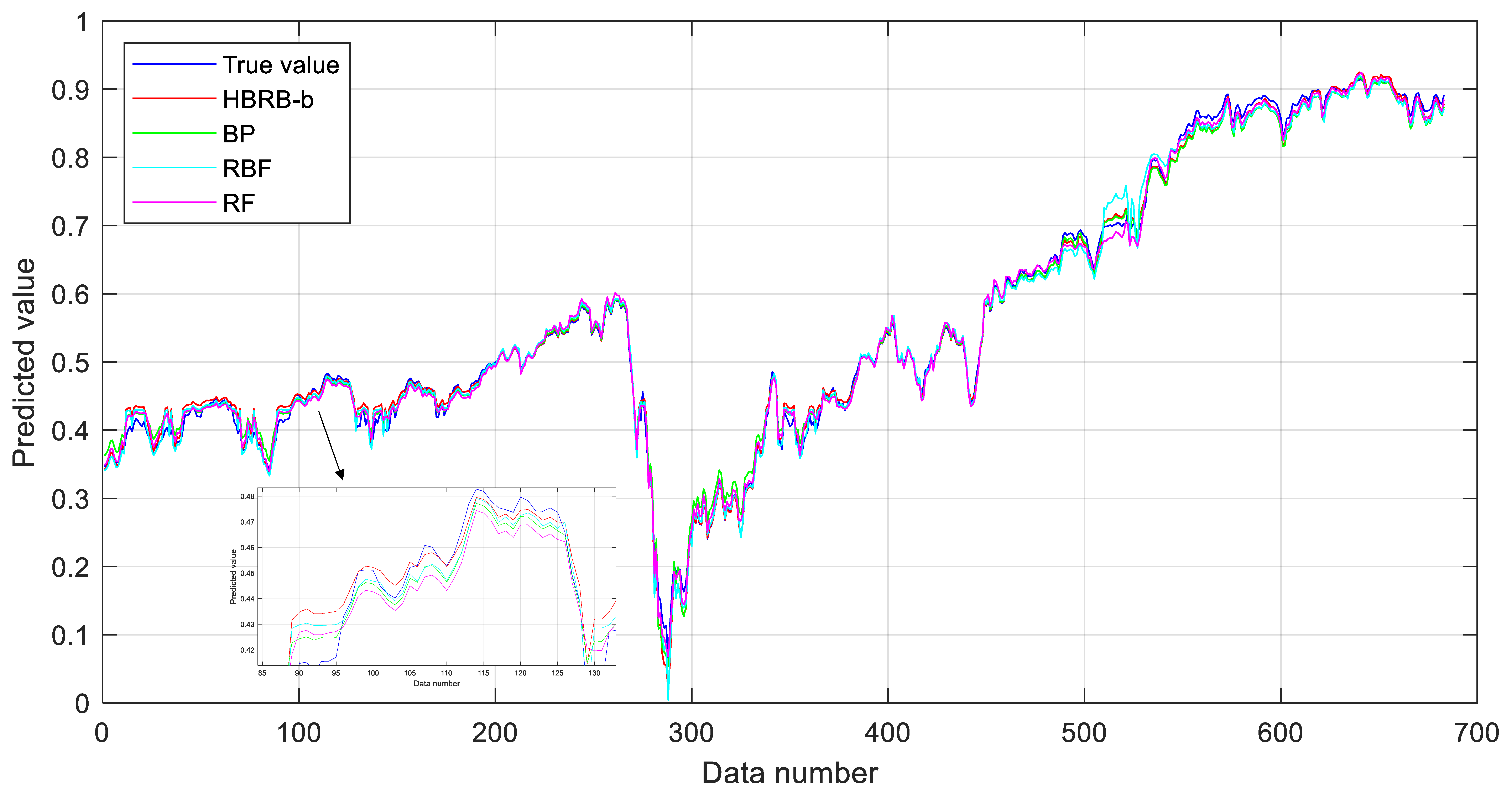
presents the comparison results of all the models. Figure 10 shows the comparison results between all BRB-based models and the actual values, and Figure 11 shows the comparison between the predicted values and the true values of HBRB-b and the other three machine learning models. Overall, the prediction curves of all models can follow the changing trend of the true values quite well. However, within the data range of 100 to 150, when the predicted values fluctuate greatly, the predicted values of the HBRB-b and RBF models are closer to the true values, showing better adaptability and accuracy. Euclidean distance is an important indicator for measuring the difference between the predicted value and the true value. The smaller its value is, the higher the prediction accuracy of the model is. Among all models listed in Table 6, the HBRB-b model achieves the best performance, with a Euclidean distance of 0.3193, while the PCMAES-BRB and DE-BRB models show distances of 1.4161 and 1.7652, respectively. The Euclidean distance of the PCMAES-BRB model is 1.4161, and that of the DE-BRB model is 1.7652, also showing good interpretability. The Euclidean distance of the WOA-BRB model is 2.8082, which is the largest among the listed models. Since BP, RBF, and RF models are essentially black-box models, they lack transparency when providing prediction results and therefore do not have inherent interpretability. Overall, the HBRB-b-based stock price prediction model demonstrates clear advantages in both accuracy and interpretability. The experimental results provide compelling evidence that validates the proposed hypotheses.

5.5.2. Robustness Analysis

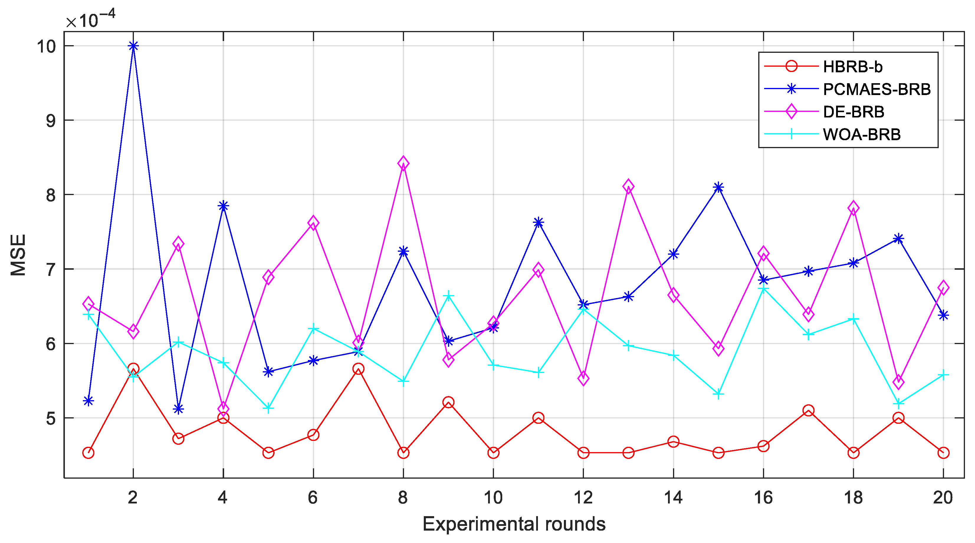
To ensure methodological robustness, a comprehensive experimental analysis was conducted involving twenty repeated optimization trials across seven comparative models: PCMAES-BRB, DE-BRB, WOA-BRB, Backpropagation Neural Network (BP), Radial Basis Function (RBF), Random Forest (RF), and the proposed HBRB-b model. The robustness analysis results are systematically presented in Appendix C.1, while Figure 12 and Figure 13 provide visual comparisons of the prediction performance through mean square error (MSE) metrics across all evaluated models.

The experimental results reveal that the HBRB-b model maintains consistently low MSE values with minimal variation across multiple experimental trials, demonstrating remarkable stability in stock price trend prediction. This stable performance stems from three fundamental improvements brought about by the interpretability criterion: first, it confines the parameter search space within reasonable bounds; second, it mitigates optimization volatility during training; and third, it ensures that optimal solutions align with domain expert knowledge. These synergistic effects not only enhance optimization efficiency but also guarantee the reliability of prediction outcomes, making the model more robust and practical for real-world financial applications.

The inherent instability of BP and RF models originates from their core algorithmic mechanisms: BP networks are highly sensitive to random weight initialization and may converge to divergent local optima during training, resulting in substantial performance variance. Similarly, while robust, RF models introduce variability through bootstrapped sampling and random feature selection at each node, meaning different random seeds can construct meaningfully different forests. In contrast, HBRB-b’s stability is engineered by its interpretability constraints, which act as a powerful regularizer. By severely restricting the parameter search space to a financially plausible and consistent region, these constraints effectively anchor the optimization process, preventing it from overfitting to stochastic noise and making its results far less dependent on random initial conditions.

For portfolio or risk managers, the stability of HBRB-b can translate into lower model risk and higher trust, as the model’s performance in real-time trading is predictable and consistent with the results of its backtesting. This reliability reduces the operational burden and cost associated with frequent model monitoring, validation, and recalibration. Ultimately, it provides decision-makers with the confidence that artificial intelligence predictions are robust and reliable.

5.5.3. Discussion on Interpretability and Practical Implications

The excellent performance of the HBRB-b model is not merely a statistical outcome but a direct result of its foundational architecture. Unlike black-box models which function as opaque function approximators, HBRB-b integrates domain knowledge through its belief rules, effectively constraining its optimization to financially plausible patterns. For instance, rules linking a high opening price with a low trading range to a bearish sentiment encapsulate classic technical analysis wisdom. The hierarchical structure mitigates the curse of dimensionality, allowing the model to capture complex interactions without overfitting the prevalent noise in market data. Furthermore, the interpretability constraints applied during optimization prevent the model from learning spurious, non-generalizable relationships, thereby enhancing its robustness in volatile markets.

The practical implications of this interpretable accuracy are profound for various financial market participants. For the quantitative analyst, the model offers a transparent tool for strategy development and validation. The ability to audit which rules activate for a given prediction enables continuous refinement of the rule base using new financial insights. For the portfolio manager, the model’s output—a belief distribution—provides a nuanced view of risk and opportunity. A prediction of (Down, 0.6), (Neutral, 0.3), (Up, 0.1) clearly communicates a high-probability downward trend with a quantified level of uncertainty, enabling more informed asset allocation and hedging decisions than a single-point estimate ever could. For regulators, the model’s transparency is a key advantage for market monitoring and stress testing, as its reasoning can be scrutinized to understand the drivers of predicted market downturns.

This stands in stark contrast to the compared black-box models. While BP, RBF, and RF can achieve competitive accuracy, their predictions are not auditable. A fund manager cannot justify a multi-million-dollar trade based on a prediction from an unexplainable neural network. The RF model, while able to rank feature importance, fails to articulate the complex conditional logic between features.

Table 7. A multidimensional comparison of model characteristics for financial prediction.

Aspect	HBRB-b	BP/RBF	Random Forest (RF)	Implication for Financial Use
Interpretability	High (gray-box)	Very low (black-box)	Medium (black-box)	HBRB-b provides rationale for decisions; others do not.
Output	Belief distribution	Point forecast	Point forecast	Only HBRB-b quantifies prediction uncertainty.
Knowledge Integration	Explicit (via rules)	Implicit (very difficult)	Implicit (very difficult)	Expert financial wisdom can be directly encoded into HBRB-b.
Overfitting Resistance	High (constrained structure)	Low	Medium	HBRB-b is more robust to market noise.
Decision Trust	High (auditable logic)	Low	Low	Essential for compliance and high-stakes decisions.
Primary Strength	Balance of accuracy and explainability	Pure function approximation	Handling nonlinear relationships	HBRB-b is designed for decision support; others for prediction only.

conducts an in-depth comparison between the HBRB-b model and other machine learning models. It can be seen that although these black-box models have strong approximation capabilities, their predictions lack the transparency required for full trust in critical financial decision-making environments. Therefore, the HBRB-b model addresses this gap by offering a solution that is accurate, actionable, and trustworthy.

6. Conclusions

Accurate prediction of stock price trends is vital for ensuring the stable operation of financial markets, optimizing resource allocation, and mitigating systemic risks. To maximize the practical utility of predictive models, they not only need to provide highly accurate prediction results but also maintain strong interpretability—this is the dual requirement emphasized in the recent literature on interpretable artificial intelligence in the financial field [11,16,35]. This work is in line with an increasing number of research institutions advocating for the establishment of transparent artificial intelligence systems in high-risk fields such as finance, but it differs from the pure black-box approach that dominates current predictive modeling [7,27]. This requires that the prediction process and results of the model be transparent and understandable, enabling decision-makers to clearly understand the underlying logic and fundamental principles behind the predictions, thereby promoting effective verification and making informed decisions under uncertain market conditions.

This research has contributed to the theoretical knowledge system in several meaningful aspects. Firstly, a hierarchical BRB structure was introduced, effectively alleviating the problem of combinatorial rule explosion, which is the fundamental limitation of traditional BRB systems in multi-attribute prediction. This structural innovation not only enhances computational efficiency but also maintains interpretability, thereby addressing the key gap in scalable gray-box modeling. Secondly, a set of interpretability optimization standards tailored for stock prediction was proposed, extending the general interpretability standards established by Cao et al. [11]. These constraints ensure that the optimized model is financially reasonable and auditable, bridging the gap between data-driven optimization and domain expertise. Finally, an improved Whale Optimization Algorithm (WOA) was developed, which combines an interpretability protection mechanism and provides a new approach to balancing accuracy and transparency in evolutionary optimization. Overall, these contributions have advanced the theory of explainable artificial intelligence in financial forecasting and provided a replicable framework for future research on high-risk and high-dimensional forecasting tasks.

Furthermore, the proposed HBRB-b model offers practical implications for various stakeholders in the financial sector. For banks and investment institutions, it provides a transparent and auditable decision-support tool for risk management and trading strategy formulation, enhancing trust in AI-driven predictions. For regulators, the model’s interpretability facilitates compliance checks and systemic risk monitoring, which supports the development of clearer guidelines for explainable AI in finance. For investors, the model delivers not only accurate forecasts but also actionable insights into market dynamics, enabling more informed and justified investment decisions.

The experimental results demonstrate that the proposed model exhibits strong performance in terms of prediction accuracy, interpretability, robustness, and generalization capability. This study has some limitations. First, the model’s interpretability partially relies on expert knowledge, potentially introducing subjectivity. Secondly, and more importantly, the model was trained and tested on an aggregated global dataset. While this dataset includes indices from various regions (U.S., Europe, Asia), the model’s efficacy when transferred directly to a specific, distinct market (e.g., focusing solely on U.S. stocks or emerging markets) warrants further investigation. Different markets exhibit unique characteristics, regulations, and participant behaviors, which may not be fully captured by a generalized model. Future work will focus on validating the model’s transferability by conducting dedicated experiments on individual markets and exploring strategies such as incorporating market-type as an input feature or developing market-specific model instances to enhance adaptability and performance in targeted financial environments.

References

1. Ho, T.T.; Huang, Y. Stock price movement prediction using sentiment analysis and CandleStick chart representation. Sensors 2021, 21, 7957. [Google Scholar] [CrossRef]
2. Vorobets, T.I. The essence of financial risks at the stock market. Actual Probl. Econ. 2012, 134, 253–257. [Google Scholar]
3. Yan, X.; Xie, C.; Wang, G. The stability of financial market networks. Europhys. Lett. 2014, 107, 48002. [Google Scholar] [CrossRef]
4. Jones, C.P.; Wilson, J.W. The changing nature of stock and bond volatility. Financ. Anal. J. 2004, 60, 100–113. [Google Scholar] [CrossRef]
5. Sheng, H. Option measures and stock characteristics. Financ. Res. Lett. 2022, 44, 102058. [Google Scholar] [CrossRef]
6. Lucey, B.M.; Muckley, C. Robust global stock market interdependencies. Int. Rev. Financ. Anal. 2011, 20, 215–224. [Google Scholar] [CrossRef]
7. Ljung, L. Black-box models from input-output measurements. In Proceedings of the 18th IEEE instrumentation and measurement technology conference. Rediscovering measurement in the age of informatics (Cat. No. 01CH 37188), IMTC 2001, Budapest, Hungary, 21–23 May 2001; Volume 1, pp. 138–146. [Google Scholar]
8. Shukla, P.K.; Aljaedi, A.; Pareek, P.K.; Alharbi, A.R.; Jamal, S.S. AES based white box cryptography in digital signature verification. Sensors 2022, 22, 9444. [Google Scholar] [CrossRef]
9. Van Can, H.J.L.; Te Braake, H.A.B.; Dubbelman, S.; Hellinga, C.; Luyben, K.C.; Heijnen, J.J. Understanding and applying the extrapolation properties of serial gray-box models. AIChE J. 1998, 44, 1071–1089. [Google Scholar] [CrossRef]
10. Chao, Z.; Shi, S.; Gao, H.; Luo, J.; Wang, H. A gray-box performance model for apache spark. Future Gener. Comput. Syst. 2018, 89, 58–67. [Google Scholar] [CrossRef]
11. Cao, Y.; Zhou, Z.; Hu, C.; He, W.; Tang, S. On the interpretability of belief rule-based expert systems. IEEE Trans. Fuzzy Syst. 2021, 29, 3489–3503. [Google Scholar] [CrossRef]
12. Zhou, Z.J.; Cao, Y.; Hu, C.H.; Tang, S.W.; Zhang, C.C.; Wang, J. Interpretability and development of rule-based modelling methods. Acta Automat. Sin. 2021, 47, 1201–1216. [Google Scholar]
13. Feng, Z.; Zhou, Z.; Hu, C.; Ban, X.; Hu, G. A safety assessment model based on belief rule base with new optimization method. Reliab. Eng. Syst. Saf. 2020, 203, 107055. [Google Scholar] [CrossRef]
14. Zhou, Z.J.; Hu, G.Y.; Hu, C.H.; Wen, C.L.; Chang, L.L. A survey of belief rule-base expert system. IEEE Trans. Syst. Man Cybern.-Syst. 2021, 51, 4944–4958. [Google Scholar] [CrossRef]
15. Zhou, Z.; Cao, Y.; Hu, G.; Zhang, Y.; Tang, S.; Chen, Y. New health-state assessment model based on belief rule base with interpretability. Sci. China Inf. Sci. 2021, 64, 172214. [Google Scholar] [CrossRef]
16. Han, P.; He, W.; Cao, Y.; Li, Y.; Mu, Q.; Wang, Y. Lithium-ion battery health assessment method based on belief rule base with interpretability. Appl. Soft Comput. 2023, 138, 110160. [Google Scholar] [CrossRef]
17. Soni, P.; Tewari, Y.; Krishnan, D. Machine learning approaches in stock price prediction: A systematic review. J. Phys. Conf. Ser. 2022, 2161, 012065. [Google Scholar] [CrossRef]
18. Mukherjee, S.; Sadhukhan, B.; Sarkar, N.; Roy, D.; De, S. Stock market prediction using deep learning algorithms. CAAI Trans. Intell. Technol. 2023, 8, 82–94. [Google Scholar] [CrossRef]
19. Fama, E.F. The behavior of stock-market prices. J. Bus. 1965, 38, 34–105. [Google Scholar] [CrossRef]
20. Zhang, W.; Zhuang, X. The stability of Chinese stock network and its mechanism. Phys. A Stat. Mech. Its Appl. 2019, 515, 748–761. [Google Scholar] [CrossRef]
21. Fama, E.F.; French, K.R. Common risk factors in the returns on stocks and bonds. J. Financ. Econ. 1993, 33, 3–56. [Google Scholar] [CrossRef]
22. Zhang, J.; Cui, S.; Xu, Y.; Li, Q.; Li, T. A novel data-driven stock price trend prediction system. Expert Syst. Appl. 2018, 97, 60–69. [Google Scholar] [CrossRef]
23. Xu, Y.; Cohen, S.B. Stock movement prediction from tweets and historical prices. In Proceedings of the 56th Annual Meeting of the Association for Computational Linguistics, Melbourne, Australia, 15–20 July 2018; Volume 1, pp. 1970–1979. [Google Scholar]
24. Akita, R.; Yoshihara, A.; Matsubara, T.; Uehara, K. Deep learning for stock prediction using numerical and textual information. In Proceedings of the 2016 IEEE/ACIS 15th International Conference on Computer and Information Science (ICIS), Okayama, Japan, 26–29 June 2016; pp. 1–6. [Google Scholar]
25. Mehtab, S.; Sen, J.; Dutta, A. Stock price prediction using machine learning and LSTM-based deep learning models. In Proceedings of the Second Symposium, SoMMA 2020, Chennai, India, 14–17 October 2020; Springer: Singapore, 2020; pp. 88–106. [Google Scholar]
26. Yang, H.; Liu, X.Y.; Zhong, S.; Walid, A. Deep reinforcement learning for automated stock trading: An ensemble strategy. In Proceedings of the First ACM International Conference on AI in Finance, online, 15–16 October 2020; pp. 1–8. [Google Scholar]
27. Cui, C.; Wang, P.; Li, Y.; Zhang, Y. McVCsB: A new hybrid deep learning network for stock index prediction. Expert Syst. Appl. 2023, 232, 120902. [Google Scholar] [CrossRef]
28. Cakra, Y.E.; Trisedya, B.D. Stock price prediction using linear regression based on sentiment analysis. In Proceedings of the 2015 International Conference on Advanced Computer Science and Information Systems (ICACSIS), Depok, Indonesia, 10–11 October 2015; pp. 147–154. [Google Scholar]
29. Nair, B.B.; Mohandas, V.P.; Sakthivel, N.R. A decision tree-rough set hybrid system for stock market trend prediction. Int. J. Comput. Appl. 2010, 6, 1–6. [Google Scholar] [CrossRef]
30. Gong, J.; Sun, S. A new approach of stock price prediction based on logistic regression model. In Proceedings of the 2009 International Conference on New Trends in Information and Service Science, Beijing, China, 30 June–2 July 2009; pp. 1366–1371. [Google Scholar]
31. Agrawal, M.; Shukla, P.K.; Nair, R.; Nayyar, A.; Masud, M. Stock prediction based on technical indicators using deep learning model. Comput. Mater. Contin. 2022, 70, 288–304. [Google Scholar] [CrossRef]
32. Li, S.; Liao, W.; Chen, Y.; Yan, R. PEN: Prediction-explanation network to forecast stock price movement with better explainability. Proc. AAAI Conf. Artif. Intell. 2023, 37, 5187–5194. [Google Scholar] [CrossRef]
33. Zhou, Z.J.; Hu, C.H.; Yang, J.B.; Xu, D.L.; Zhou, D.H. Online updating belief rule based system for pipeline leak detection under expert intervention. Expert Syst. Appl. 2009, 36, 7700–7709. [Google Scholar] [CrossRef]
34. Yin, X.; He, W.; Cao, Y.; Zhou, G.; Li, H. Interpretable belief rule base for safety state assessment with reverse causal inference. Inf. Sci. 2023, 651, 119748. [Google Scholar] [CrossRef]
35. Cao, Y.; Tang, S.; Yao, R.; Chang, L.; Yin, X. Interpretable hierarchical belief rule base expert system for complex system modeling. Measurement 2024, 226, 114033. [Google Scholar] [CrossRef]
36. Nadimi-Shahraki, M.H.; Zamani, H.; Asghari Varzaneh, Z.; Mirjalili, S. A systematic review of the whale optimization algorithm: Theoretical foundation, improvements, and hybridizations. Arch. Comput. Methods Eng. 2023, 30, 4113–4159. [Google Scholar] [CrossRef]
37. Liu, L.; Zhang, R. Multistrategy improved whale optimization algorithm and its application. Comput. Intell. Neurosci. 2022, 2022, 3418269. [Google Scholar] [CrossRef]
38. Chakraborty, S.; Sharma, S.; Saha, A.K.; Saha, A. A novel improved whale optimization algorithm to solve numerical optimization and real-world applications. Artif. Intell. Rev. 2022, 55, 4605–4716. [Google Scholar] [CrossRef]
39. Uzer, M.S.; Inan, O. Application of improved hybrid whale optimization algorithm to optimization problems. Neural Comput. Appl. 2023, 35, 12433–12451. [Google Scholar] [CrossRef]
40. Qu, S.; Liu, H.; Xu, Y.; Wang, L.; Liu, Y.; Zhang, L.; Song, J.; Li, Z. Application of spiral enhanced whale optimization algorithm in solving optimization problems. Sci. Rep. 2024, 14, 24534. [Google Scholar] [CrossRef] [PubMed]
Figure 1. Stock price trend prediction model based on HBRB-b.
Symmetry 17 01550 g001
Figure 2. Examples of reasonable and unreasonable belief distributions in stock trend prediction.
Symmetry 17 01550 g002
Figure 3. Flowchart of WOA with interpretability constraints.
Symmetry 17 01550 g003
Figure 4. Normalized input attributes (Open, Close, High, Low) and their relationship with the next day’s closing price.
Symmetry 17 01550 g004
Figure 5. Structure of stock price trend prediction model based on HBRB-b.
Symmetry 17 01550 g005
Figure 6. Prediction performance of the optimized HBRB-b model on test data.
Symmetry 17 01550 g006
Figure 7. The belief distribution of the HBRB-b and WOA-BRB rules.
Symmetry 17 01550 g007
Figure 8. Comparison of the belief distribution of PCMAES-BRB rules.
Symmetry 17 01550 g008
Figure 9. Comparison of the belief distribution of DE-BRB rules.
Symmetry 17 01550 g009
Figure 10. A comparison of all BRB-based models.
Symmetry 17 01550 g010
Figure 11. Compare with other machine learning models.
Symmetry 17 01550 g011
Figure 12. Comparison of the MSE with all BRB models.
Symmetry 17 01550 g012
Figure 13. Comparison of MSE with other machine learning models.
Symmetry 17 01550 g013