Article

Application of an Improved Double Q-Learning Algorithm in Ground Mobile Robots

1
College of Mechatronics Engineering, North University of China, Taiyuan 030051, China
2
Faculty of Science and Engineering, BEng Electrical & Electronic Engineering, University of Liverpool, Brownlow Hill, Liverpool L69 7ZX, UK
*
Author to whom correspondence should be addressed.
Symmetry 2025, 17(9), 1530; https://doi.org/10.3390/sym17091530
Submission received: 30 April 2025 / Revised: 4 July 2025 / Accepted: 7 July 2025 / Published: 12 September 2025

Abstract

Highlights

What are the main findings?
  • An improved algorithm was developed for unmanned ground robots, which has stronger anti-interference and noise resistance capabilities.
  • The algorithm can quickly find the shortest path and precisely avoid all obstacles.
What are the implications of the main findings?
  • The algorithm has excellent application effects in complex environments.
  • It can enhance the ability of unmanned ground robots to perform tasks and improve efficiency.

Abstract

Since efficient path planning technology is the key to the safe and autonomous navigation of autonomous ground robots, and in the complex and asymmetrically distributed land environment, the existing path planning and obstacle avoidance technologies seem somewhat inadequate. Since efficient path planning technology is key to the safe and autonomous navigation of autonomous ground robots, an advanced double Q-learning algorithm based on self-supervised prediction and curiosity-driven exploration is proposed. The algorithm reduces the risk of overestimation and bootstrapping by adjusting the calculation method of the target Q value and optimizing the network structure. In addition, a priority experience replay is introduced to set the priority for the data in the experience pool, thereby increasing the probability that better data is extracted. Experience pool data with fewer training times can be used more effectively. Adding the curiosity network to the original neural network, each state is given an overall reward when performing diverse actions. This method enhances the exploration of unmanned ground mobile robots and can independently select the shortest path to the endpoint. In complex environments, compared with the Sparrow Search Algorithm, Dung Beetle Optimization Algorithm, and Particle Swarm Optimization Algorithm, the results of the proposed algorithm are reduced by 18.07%, 7.91%, and 5.56%, respectively. Therefore, it could better cope with the challenges brought by complex environments and solve the problem that the algorithm cannot converge in complex environments.

1. Introduction

As a significant part of the unmanned ground mobile platform, ground mobile robots should have stable motion and good load functions. It is crucial to investigate autonomous ground mobile robots. The safe navigation ability of GMRs in complex land environments depends on the effective application of autonomous navigation and obstacle avoidance technology. The safe navigation ability of GMRs in complex land environments depends on the effective application of autonomous navigation and obstacle avoidance technology. But nowadays, the ground environment has become full of uncertainties and asymmetries. In order to ensure the efficient and safe operation of land resource exploration tasks, it is crucial to study path planning technology [1,2,3,4].
The ultimate goal of a path planning algorithm is to find an optimal path between the starting point and the end point of the target. These algorithms can be placed into three categories: traditional path planning algorithms, sampling-based path planning algorithms, and intelligent bionic path planning algorithms [5,6,7]. The traditional path planning algorithm refers to the leverage of pre-set map information and a fixed algorithm to determine the best path from the starting point to the end point [8,9,10]. Commonly used algorithms are the Dijkstra algorithm, the rapidly-exploring random tree (RRT) algorithm, and so on [11]. Among them, the Dijkstra algorithm searches for feasible nodes from the starting point in path planning, and calculates the distance to the starting point until the target point is found to obtain the shortest path. However, the number of search nodes is numerous, resulting in low efficiency and a lack of smoothness [12,13,14,15,16]. The algorithm combines the Dijkstra algorithm with BFS, and quickly finds the optimal path by adding a heuristic function [17]. However, the algorithm has high memory requirements and poor performance when dealing with large-scale problems or complex maps [18]. The rapidly-exploring random tree algorithm quickly searches for a path from the starting point to the target point, but has low efficiency and does not find the optimal path [19]. In general, these traditional methods have limitations in dealing with land environments, especially in the face of complex and changeable situations where there will be a variety of different problems, so path planning is gradually developing in a more intelligent direction. The intelligent bionic path planning algorithms arose at the historic moment [20]. These algorithms include a genetic algorithm and an ant colony algorithm, but both have local optimal problems. It is necessary to pre-set the environment on the land and the mobile robot model, which limits their adaptability in unknown environments [21,22]. In Reference, a particle swarm optimization algorithm based on path smoothing adaptive parameters is proposed to solve the optimal path of a mobile robot. In Reference [23], a genetic algorithm based on natural genetic mechanisms and biological evolution theory, such as selection, is used for path planning, but the algorithm may converge prematurely and fall into a local optimum. Based on the bionic neural network architecture, References [24,25] employed a dynamic neural network model for path planning, which is suitable for complex and harsh environments such as strong winds and heavy rain. However, these intelligent methods fail to construct the kinematics or dynamics model of the agent in advance, and do not obtain information about the place where the task needs to be performed. Therefore, it is difficult to apply them in terrestrial environments with unknown environmental information or significant changes [26].
Artificial intelligence and machine learning technologies are developing rapidly, and people are paying more and more attention to this field. Among these technologies, machine learning provides more choices and possibilities for dealing with the path planning problems of unmanned mobile robots. Reinforcement learning is a branch of machine learning that aims to learn optimal strategies by interacting with the environment. By adjusting their behavior according to the reward signal of environmental feedback to maximize long-term returns, GMRs can continuously optimize their decision-making in complex environments and show flexible adaptability through this self-learning approach [27,28]. It performs well in land applications, especially in the application of mobile robots. In reinforcement learning, commonly used algorithms include Q-learning and deep Q-network algorithms [29]. The DQN algorithm opens up a new research direction for intelligent agents in complex environments. It combines the characteristics of deep learning and reinforcement learning, provides a new idea for the path planning of GMRs in high-dimensional complex environments, and solves the control problem, but the algorithm’s path planning is inefficient and not stable enough [30].
In the exploration method, compared with traditional methods such as ε-greedy or Boltzmann exploration, the curiosity mechanism is more targeted and efficient in theory, which is mainly reflected in the following aspects: 1. Goal orientation vs. random exploration. Traditional methods (ε-greedy, Boltzmann) randomly select actions under a certain probability and try to explore new states. However, this kind of exploration lacks goal orientation and may repeatedly explore known or invalid areas, with low efficiency. Curiosity mechanism: Intrinsic rewards guide agents to explore ‘unknown’ or ‘unpredictable’ states, which is more targeted. The focus of exploration is on high-uncertainty areas, thereby improving the quality of exploration. 2. Intrinsic motivation-driven learning. Traditional methods rely only on external rewards to learn strategies. If external rewards are sparse or delayed, exploration will stagnate; the curiosity mechanism introduces intrinsic motivation. Even if there are fewer external rewards, agents can actively explore to improve their understanding of the environmental model, and it is easier to find long-term beneficial strategies. 3. Information gain maximization. In theory, the curiosity mechanism can be regarded as an attempt to maximize the information gain or prediction error, similar to the exploratory part of Bayesian optimization. 4. Avoid falling into a local optimum. Methods such as ε-greedy are easy to fall into local optimal strategies due to high utilization in the later stage; the curiosity mechanism can still maintain the exploration power of the unknown area in the later stage of training, helping the agent jump out of the local optimum and find a better solution [31,32].
In view of the problems existing in the above methods, this paper proposes a method combining a curiosity mechanism with DQN. Different from other algorithms, it has a relatively stable noise reduction ability and always chooses the optimal route in a complex environment to reach the endpoint. In general, the contributions of this paper are summarized as follows:
(1)
Analyze the limitations of existing path planning algorithms, and introduce a competitive network and curiosity mechanism to break through the limitations.
(2)
The main idea of the proposed method is to combine it with the competitive network and the curiosity module to improve its stability and path planning ability, and to solve the problem of convergence too early and too late.
(3)
Establish a suitable environment model for the smooth progress of the simulation experiment and provide a wide range of comparison results to prove the advantages of the algorithm. In addition, Sparrow Search Algorithm (SSA), Dung Beetle Optimization Algorithm (DBO), and Particle Swarm Optimization Algorithm (PSO) were simulated in the same environment to verify the feasibility of the algorithm.
The rest of this paper is organized as follows. The second section briefly summarizes the basic concepts and formulas of related algorithms and competitive networks; the third section introduces the relevant knowledge of path planning combined with internal rewards; in the fourth section, the environment required for the experiment is modeled and simulated, and the results are analyzed. Finally, the fifth section provides comments and discusses future work.
The following are the symbols used in this article and their meanings:
Let s be the current state, a the current action, r the reward, s the next state, α the learning rate, and γ the discount factor. There are two independent Q-functions, denoted as Q A and Q B . max a A Q ( s t + 1 , a ; w ) represents the maximum action value estimated by the target network. y ˜ t denotes the TD target in double Q-learning, and y ˜ t also refers to the maximum action value computed by the target network. V * ( s ) is the optimal state-value function. π represents a deterministic policy. U ^ ( a t ) is a measure of uncertainty, and p is a probability that gradually decays over time.

2. Construction of Double Q Algorithm

2.1. Double Q-Learning

Double Q-learning is an improved version of the traditional DQN algorithm that alleviates the overestimation caused by maximization. The algorithm flow is shown in Figure 1. In Q-learning, since the update process depends on maximizing the action value function, the estimation of the Q value is often high. Among them, the action value function Q ( s , a ) is iteratively updated by the update rule of Equation (1):
Q ( s , a ) = Q ( s , a ) + α [ R + γ max a Q ( s , a ) Q ( s , a ) ]
where Q ( s , a ) is the estimated value (i.e., Q value) of the action a under the current state s; α is the learning rate and the value range is 0 , 1 ; R is the instant reward obtained after performing action a under state s; γ is the discount factor; max a Q ( s , a ) is the maximum Q value of all possible actions a’ in the next state s’; and Q ( s , a ) + α is the update of the current Q value to the new target value, where the target value is R + max a Q ( s , a ) .
Among them, s is the current state, a is the current action, r is the reward, s is the next state, α is the learning rate, and γ is the discount factor.
In order to solve the overestimation problem, double Q-learning introduces two independent Q functions, denoted as Q A and Q B . These two functions are alternately used for action selection and Q value update. At each time step, select an action according to the current strategy. For example, if Q A is used for action selection, the Q A ( s , a ) is selected as the largest action.
Using another Q function to update the Q value of the selected action. If the action is selected based on Q A , then use Q B to update the Q value, and vice versa. The update rule becomes:
Q A ( s , a ) = Q A ( s , a ) + α [ R + γ Q B ( a r g m a x a Q A ( s , a ) , s ) Q A ( s , a ) ]
where s is the current state; a is the current action taken; s’ is the next state after the execution of action a; Q A and Q B are two independent Q functions, where Q A is the Q function that is currently being updated, and Q B is used to evaluate the value of the best action in the next state to prevent overestimation; and arg max a Q A ( s , a ) is in the state s’, select the action that maximizes the value of Q A .
Here, a r g m a x a Q A ( s , a ) represents that in the state of s , the action is selected according to Q A .
Through the value network, the maximum action is selected under the state of s t + 1 , and the target network estimation is used to estimate Q * ( s t + 1 , a ) and the TD target value.
If Q ( s t + 1 , a * ; w ) represents the maximum action value of double Q-learning, and max a A Q ( s t + 1 , a ; w ) denotes the maximum action value using the target network, then:
Q ( s t + 1 , a * ; w ) max a A Q ( s t + 1 , a ; w )
Then:
y ¯ t y ¯ t
y ¯ t represents the TD goal of double Q-learning, and y ¯ t denotes the maximum action value of using the target network. Formula (4) shows that using double Q-learning gets a smaller TD target, thereby reducing the overestimation problem.

2.2. Dueling Network

2.2.1. Optimal Advantage Function

The optimal dominance function is defined as:
A * ( s , a ) = Q * ( s , a ) V * ( s )
Here, V * ( s ) is the optimal state value function, defined as:
V * ( s ) = max π V π ( s )
According to (5), the optimal action function is:
Q * ( s , a ) = V * ( s ) + A * ( s , a )
For a deterministic strategy π , there exists:
V * ( s ) = max a Q * ( s , a )
It can be obtained:
max a Q * ( s , a ) V * ( s ) = 0
The optimal action function can be obtained from Formulas (5) and (9):
Q * ( s , a ) = V * ( s ) + A * ( s , a ) max a A * ( s , a )

2.2.2. Dueling Network Architecture

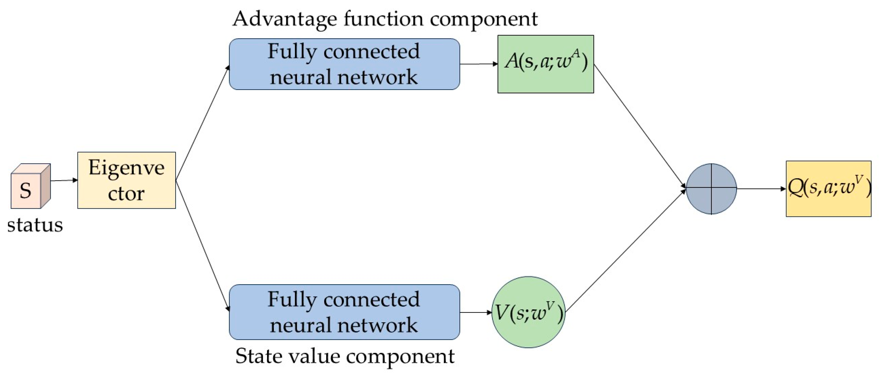
The competition network consists of two neural networks, one of which is the advantage function network, denoted as A * ( s , a ; w A ) . Another neural network is denoted as V ( s ; w V ) , which is an approximation of the optimal state value function V * ( s ) . By replacing V * and A * with the corresponding network in Formula (10), the neural network of the optimal action value function Q * can be constructed as follows:
Q * ( s , a ; w ) = V * ( s ; w V ) + A * ( s , a ; w A ) max a A * ( s , a ; w A ) , w = ( w V , w A )
Its network structure is shown in Figure 2.
The upper part of the figure estimates the dominance function, and the lower part estimates the value function. The input of both is the feature vector of state s. After the processing of the competitive network, the final output is the action value. The training of competitive networks is usually the same as that of DQN, so dueling networks and double Q-learning can be combined to form a more stable algorithm than DDQN.

3. Path Planning Combined with Intrinsic Rewards

In reinforcement learning, a GMR obtains the maximum cumulative reward in an unknown environment by trial and error. Since the environment has not yet been fully explored, the GMR faces the challenge of action selection. The key lies in balancing exploration and exploitation: both acquiring new knowledge and using existing information to obtain rewards, so as to continuously optimize decision-making strategies.

3.1. Reinforcement Learning Exploration

3.1.1. Classical Exploration Methods

In the complex environment of reinforcement learning, in order to effectively deal with the trade-off between exploration and exploitation, researchers have proposed a variety of exploration strategies to find the best balance between exploration and exploitation. Common strategies include Epsilon-greedy, Boltzmann distribution, and the upper confidence bound (UCB) algorithm.
The core idea of the Epsilon-greedy strategy is that when making decisions, the agent randomly selects an unknown action with the probability of a small positive ε ( ε < 1 ), and selects the currently considered optimal action with the probability 1 ε . Specifically, assuming that in a certain state s t S , the intelligent agent chooses the set of actions A , according to the ε –greedy strategy, the probability that each action is selected is ε / A , where A is the size of the action set. This means that each action has an equal probability of ε / A to be selected non-greedily. With the probability of 1 ε , the intelligent experience selects the action with the highest valuation in the current state. Therefore, the total probability of the greedy strategy is 1 ε + ε / A . The cleverness of this design is that even if the greedy strategy is selected most of the time, it still selects non-greedy actions with a certain probability, ensuring that each action has a chance to be explored. By reasonably balancing exploration and exploitation, the ε –greedy strategy provides a feasible framework for reinforcement learning algorithms, in which agents explore the environment comprehensively and effectively in the learning process, so as to gradually improve the decision-making strategy.
The Boltzmann distribution strategy is derived from the energy distribution principle of statistical physics. The behavior selection of the agent is controlled by the temperature parameter: the random exploration is increased when the temperature is increased. The high-return action is emphasized when the temperature is decreased so as to balance the contradiction between exploration and utilization in machine learning, as shown in Formula (12).
p i ( t + 1 ) = e μ i ( t ) / τ j = 1 k e μ j ( t ) / τ , i = 1 n .
μ i ( t ) represents the mean value of reward for each action, τ denotes the temperature constant in physics, and Formula (12) represents the random coefficient, which is mainly used to control the probability of exploration and exploitation. At that time, the system inclined towards choosing those actions with higher average rewards and implementing utilization strategies. The system also tended to explore new actions to understand the environment more comprehensively; that is, it was more inclined to implement exploration strategies.
The key to the Boltzmann distribution strategy lies in the adjustment of temperature parameters. By adjusting the temperature to balance exploration and utilization, the intelligent agent adapts to the environment more flexibly. This method, based on the greedy strategy, explores the route according to the average reward of the action, reducing randomness. However, due to the difficulty of adjusting the hyperparameters, it may lead to non-convergence or over-fitting. The computational cost is high, so the effect is not ideal.
In the task of reinforcement learning, the greater the uncertainty of an action, the more valuable it is to explore. After exploration, the expected rewards are ideal. The upper confidence bound (UCB) algorithm is a policy algorithm based on uncertainty, using Hoeffding’s inequality. The core idea is that in the existing expectation, the uncertainty measure is added, and the smaller probability is set according to the Hoeffding inequality, which is used to exceed the upper bound of the expectation. Generally, it decreases with time and could be set as follows:
p = e 2 N ( a t ) U ^ ( a t )
U ^ ( a t ) = log p 2 ( N ( a t ) )
p is the probability of gradually decreasing; N ( a t ) counts the number of times the action a has been selected up to the current moment t ; and U ^ ( a t ) is the uncertainty measure, or the confidence. The number of initial selections is 0, avoiding the divisor of 0, adding an additional 1, and substituting p = 1 t at the same time.
U ^ ( a t ) = log t 2 ( N ( a t ) ) + 1
Then, the final selection strategy changes from expectation Q ^ ( a ) -based to UCB-based. c is the coefficient, which is used to control the proportion of uncertainty measures and can be set to 1; that is:
a t = arg m a x a A [ Q ^ a ]
a t = arg m a x a A Q ^ a + c U ^ ( a t )
The first item in this formula is an estimate of the value of the action up to the present time t, representing the realistic part of the likelihood of being the optimal action. Formula (17) shows that if an action is selected more times, it means that the uncertainty of its action value estimation is smaller. If an action is selected zero times, it means that the action should be selected with the highest priority in the exploration.

3.1.2. Exploration Based on Internal Rewards

In complex environments, agents often encounter difficulties in exploration, mainly due to sparse or even misleading reward signals. In order to solve this problem, a simple approach is to manually design rewards to guide agent designers to pay attention to states that are considered important. However, this approach has limitations because it requires the designer to have a sufficient understanding of the environment, which may limit the learning potential of the agent and even lead to inappropriate behavior.
Deep reinforcement learning solves this problem by introducing an internal reward mechanism to motivate agents to explore without external rewards. This method is inspired by human intrinsic motivation, which is similar to how humans actively explore novelty due to curiosity. Through internal rewards, agents can obtain learning signals without explicit external rewards and adapt to the environment more flexibly. In this way, agents no longer rely too much on artificially designed rewards and better understand the environment. Commonly used exploration methods include count-based models and prediction-based models.
The counting-based exploration model draws on the idea of the UCB algorithm and encourages agents to actively explore novel states. The model promotes agents to explore unknown fields in depth by assigning higher internal rewards to new states. For states that have been encountered, the model gives a lower intrinsic reward and reduces the incentive to explore. Therefore, the key is to accurately judge the novelty of the state and allocate the intrinsic rewards accordingly. The intrinsic reward is shown in Formula (18).
r t i = 1 N ( s t )
There is an inverse relationship between the number of visits and the exploration reward, and the internal reward will guide the agent to choose a state with fewer visits. This method shows effective exploration resulting in a tabular environment or a simple environment. However, in the case of dealing with high-dimensional continuous state space, it is impractical to count each state accurately, and it is difficult to encounter exactly the same two states, resulting in N ( s t ) always being 0 or 1. In response to this problem. Bellemare et al. [33] proposed a density model to estimate the access frequency of the state and derived a pseudo-count of the state based on the access frequency. Tang et al. [34] proposed Locality-Sensitive Hashing (LHS) to map continuous, high-dimensional states to discrete hash codes to solve the problem of sparse non-zero states. During the training process, the agent uses LHS to map similar states to the same hash code, and counts the number of times corresponding to the hash code as the number of visits to similar states, which is used to calculate the intrinsic reward incentive exploration.
Different from the counting-based exploration model, the prediction-based exploration model defines the exploration reward as the agent’s cognition of the environment, rather than the frequency of state occurrence. In this model, the intrinsic exploration reward mainly reflects the agent’s familiarity with the dynamic changes of the environment, which can be measured by the estimation of the prediction model. Specifically, the prediction-based exploration model enables the agent to predict the future state of the environment by establishing a prediction model of the environment. When the agent can accurately predict the change of the environment, the system will give it a lower exploration reward. For cases where the difference between the predicted result and the actual result is large, the agent will receive a higher exploration reward, prompting it to explore more actively. Stadie [35] et al. first combined similar ideas with deep reinforcement learning algorithms, which encode the input state of the image into low-dimensional information through an automatic encoder and use a simple multi-layer perceptron (MLP) as a prediction model. They input the action and encoded state to predict the encoding of the next state, and calculate the intrinsic reward based on the difference between the predicted value and the encoding of the real next state. However, due to the randomness of the state changes in the environment, sometimes some state changes are not directly affected by the behavior of the agent. It is very difficult to directly predict the next state of the environment, and these state changes that are not controlled by the behavior of the agent are not actually objects that the agent can actively explore. Therefore, how to eliminate this uncontrolled state information is a key point of the prediction-based exploration model.

3.2. The Curiosity Mechanism of Self-Monitoring Prediction

The curiosity mechanism is designed to stimulate agents to take action to reduce their uncertainty about the consequences of their own behavior.
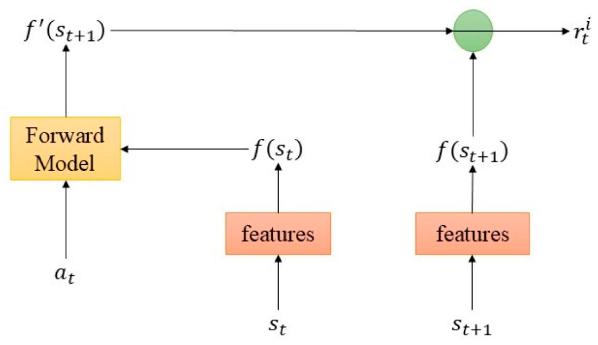
In order to obtain the curiosity error, it is necessary to construct an environmental dynamic model that predicts the next state given the current state and action. Typically, this process is implemented using the intrinsic curiosity module (ICM) to generate the agent’s curiosity rewards. The ICM includes a forward model and a reverse model, where the forward model is responsible for generating curiosity rewards, as shown in Figure 3.
The input of ICM is the state s t and s t + 1 , which are converted into feature vectors f ( s t ) and f ( s t + 1 ) through modules. The forward model uses f ( s t ) and action a t to predict the next state f ( s t + 1 ) . Subsequently, the curiosity reward r t i is calculated by comparing f ( s t + 1 ) and f ( s t + 1 ) , and the mean square error (MSE) is used to evaluate the reward during the training process. Suppose that the training forward model neural network is equivalent to the learning function f, then it is defined as:
s ^ t + 1 = f ( s t , a t ; θ 1 )
In the ICM, the quality of the feature space affects whether the prediction error can correctly measure the curiosity, so the correct feature space setting is crucial. There are three conditions that affect GMR observation:
  • Things that can be controlled by the GMR.
  • Things that the GMR fails to control but may have an impact on.
  • Things that the GMR fails to control and has no effect on.
A good curiosity feature space should be modeled for Formulas (1) and (2), and not affected by (3).
In the path planning of a GMR, combined with the previous reward function setting method, in the curiosity-driven reinforcement learning algorithm, the reward function can be designed as Formula (20):
R = r e + r i + r e + r l
where R is the reward function; r e denotes the external reward that GMR obtains in interacting with the environment; and r i is the intrinsic reward that guides GMR exploration.
In the global path planning of GMR, we hope to predict the changes caused only by GMR behavior in the environment through rule training in the feature space, ignoring other effects. Therefore, a general feature representation learning mechanism is needed to make the prediction error truly reflect the intrinsic reward signal. The inverse model uses self-supervised learning. The basic principle is to predict the action that the GMR will perform according to the current state and the next state.
The inverse model takes the feature vector ϕ ( s t ) of the state, ϕ ( s t + 1 ) as input, and predicts the GMR from the state to s t + 1 the action taken a t . Assuming that training this neural network is equivalent to learning function g, it is defined as:
a ^ t = g ( s t , s t + 1 ; θ 2 )
The whole inverse model is optimized by predicting the action a ^ t and the real action a t , that is:
min θ I L I ( a ^ t , a t )
L 1 is a loss function that measures the difference between the predicted behavior and the actual behavior.
For Equations (18)–(22) and Figure 3, the following pseudo-codes can be summarized:
# Initialize the forward model θ 1 , the strategy network π , and the reverse prediction model θ 2 . (optical)
initialize_forward_model( θ 1 )
initialize_policy_network( π )
initialize_inverse_model( θ 2 ) # optical
initialize_feature_encoder()
for episode in range(num_episodes):
s t = env.reset()
 for t in range(max_steps_per_episode):
  # 1. Select action a t according to current state s t (use policy π )
   a t = π .select_action( s t )
  # 2. Perform action a t , get the next state and external rewards
   s t + 1 , r e , done, _ = env.step( a t )
  # 3. Feature extraction (for forward prediction and reward evaluation)
   f ( s t ) = feature_encoder( s t )
   f ( s t + 1 ) = feature_encoder( s t 1 )
  # 4. The forward model predicts the next state feature
   f ( s t + 1 ) _pred = forward_model.predict( f ( s t ) , a t )
  # 5. Intrinsic reward calculation (based on prediction error or access frequency)
  prediction_error = compute_error( f ( s t + 1 ) _pred, f ( s t + 1 ) )
  visit_bonus = 1/sqrt(state_visit_count[ s t ])
   r i = prediction_error + visit_bonus
  # 6. Calculate total rewards
  R = r e + r i + exploration_reward + path_reward # Weighted fusion
  # 7. Training Strategy Network
   π .update( s t , a t , R, s t + 1 )
  # 8. Update the forward model (supervised learning)
  forward_model.update( f s t , a t , f s t + 1 )
  # Optional: train the reverse action prediction model (Inverse model)
  inverse_model.update( s t , s t + 1 , a t )
  # State update
   s t = s t + 1
  if done:
   break
In the framework of the combination of the DDQN algorithm and the ICM, the online network and the target network, as well as the parameters of the ICM, are first initialized to predict the next state and generate curiosity rewards. When the GMR interacts with the environment, the collected experience data is stored in the experience playback buffer to improve learning efficiency. The ICM generates curiosity rewards based on prediction errors to encourage exploration. The GMR leverages the online network to select the actions with the maximum Q value and record the results, while periodically copying the online network parameters to the target network to maintain stability. Using the target network to evaluate the value of behavior and update the Q value is the core of DDQN. In this way, the GMR gradually optimizes strategies, tends to explore the unknown, and accelerates the learning process. Combining the ICM with the DDQN algorithm creates a more powerful GMR, which can not only learn effective strategies through DDQN but also use ICM to enhance the ability to explore unknown environments.
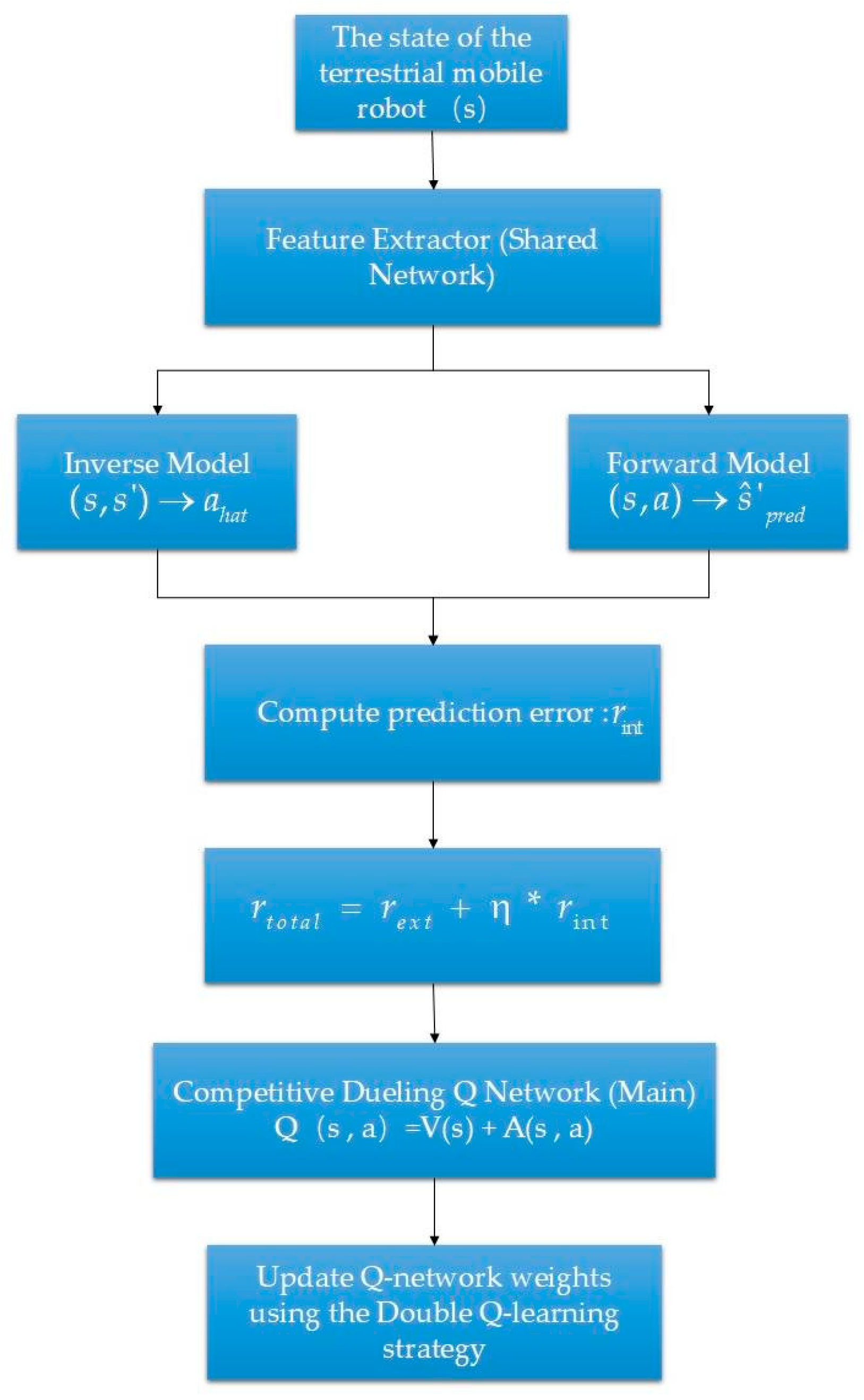
Through the content of this chapter and the previous chapter, he combination of the curiosity mechanism and competitive network in the GMR with Double Q-learning algorithm is shown in the following flow chart (Figure 4).
The current state of the ground mobile robot is the input of reinforcement learning. Information such as position, attitude, etc., can be obtained through the odometer IMU; the environmental sensing data can be obtained by a laser radar or a depth camera. These states are the basis of the whole system of learning and decision-making. Encode the original input state and output a more compact high-dimensional feature representation. This network is shared by subsequent modules (Inverse Model, Forward Model, Q network) to avoid redundant calculation and enhance feature consistency. The important components of the ICM (intrinsic curiosity module) are the reverse model and the forward model. The inverse model is used to infer which action the robot performs from the current state s and the next state s . This can enhance the predictability of state representation. The forward model attempts to predict the feature representation of the next state based on state s and action a. The core of the ICM’s internal reward mechanism is:
r int = ϕ ( s ) ϕ ( s ^ ) 2
ϕ ( s ) : the characteristics of the actual next state; ϕ ( s ^ ) : for the next state feature predicted by the forward model, the larger the error, the more ‘novel’ the exploration in the current state, and the greater the reward. r e x t is the external reward of the environment; r int are intrinsic rewards from ICM; and η is the weighting coefficient. The Q value is decomposed into: V ( s ) : state value; and A ( s , a ) : action advantage function.

4. Algorithm Simulation and Verification

4.1. Environment Model Building

By building a grid environment model in Matlab and performing GMR path planning, the effectiveness of the dual Q learning algorithm combined with the competitive network is verified. The neural network model is mainly constructed under the Pytorch machine learning framework, and three environmental models are created using the Gym module to test the algorithm.
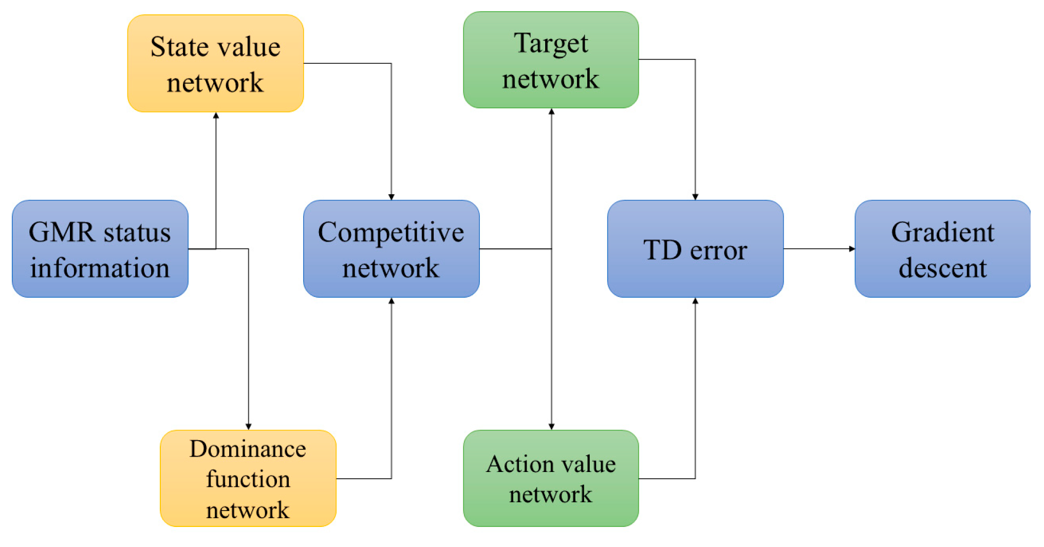
In the double Q-learning training combined with a competitive network, a 3 × 64 * * 32 × 4 neural network model is designed. The input is the coordinate information of state S and the angle between GMR and the north direction, and the output is the Q value of the four directions. The ε –greedy strategy is used to select the action, guide the behavior of the GMR in state S, obtain a new state S , and complete the environmental interaction. The training process of the neural network is shown in Figure 5.
The value of TD error is used as the loss function value of the neural network training process, and its expression is:
L q = 1 2 Q * ( s t , a t ) [ r t + γ max A Q * ( s t + 1 , A ) ] 2
where Q * ( s t , a t ) is the estimated Q value, r t + γ max A Q * ( s t + 1 , A ) is the target Q value, and Q * ( s t + 1 , A ) is estimated by the target network. During the whole training process, the target network remains unchanged and does not perform gradient descent, but regularly copies the parameters of the action value network to the target network.
In the curiosity module, a 6 × 64 × 4 complex model is designed to predict the action, and a 7 × 64 × 3 forward model is set up to predict the next state. In the training process, the reward value is set by combining the curiosity network and the external reward, and the double Q network is used for action selection to achieve GMR training.
The loss function of the forward model is designed as:
L F = ( s t + 1 s ^ t + 1 ) 2
s t + 1 is the actual state value, and s ^ t + 1 is the next state value predicted by the forward model. The inverse model loss function is designed as:
L I = i a t log a ^ t
s t + 1 is the actual action, and s ^ t + 1 is the action predicted by the reverse model.
The loss function of the double Q network is designed as:
L q = 1 2 Q * ( s t , a t ) [ r t + γ max A Q * ( s t + 1 , A ) ] 2
The overall loss function is designed as Formula (21), where β is 0.8.

4.2. Simulation Parameter Setting

In the process of training the GMR model by using the Improved Algorithm, PSO, SSA, and DBO, which integrates the competitive network architecture and combines the curiosity reward mechanism, scientific and reasonable hyperparameter configuration is the key factor to improving the efficiency of the algorithm, as it directly affects the convergence speed and final performance of the model. The parameter settings are as shown in Table 1.
In the GMR training process, a dynamic ε –greedy strategy is used to explore. This strategy randomly selects unknown actions with a small probability in each training phase, and selects the action with the maximum action value from the known actions with the remaining probability. The initial value of the exploration strategy is set to 0.7. As the training progresses, when the training schedule reaches (i_episode/TOTAL) > 0.4, ε 0.3 , the exploration probability is reduced. When the training schedule further increases to (i_episode/TOTAL) > 0.8, ε 0.35 , the exploration probability is finally adjusted to 0.05. The design of this strategy makes it possible to fully explore the unknown environment in the early stage of the GMR training process, and to plan the path more quickly in the later stage, thereby improving the learning efficiency and performance of the algorithm. In addition, the proportion of forward loss, the proportion coefficient of internal reward, and the proportion coefficient of external reward are used to adjust the reward obtained by GMR in the training process. Curiosity is designed to drive GMR to explore actively, so ε remains 0.9 throughout the training process.

4.3. Simulation Experiment

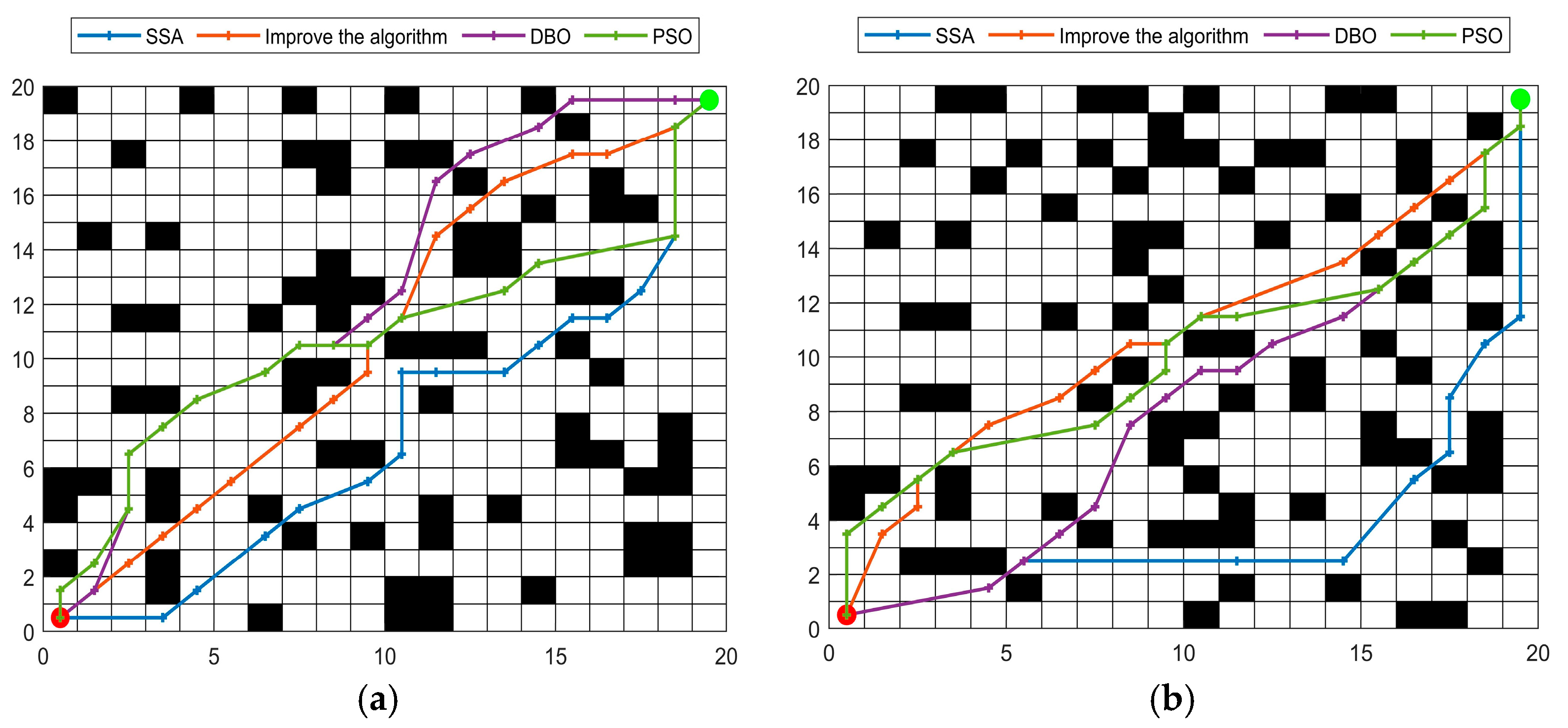
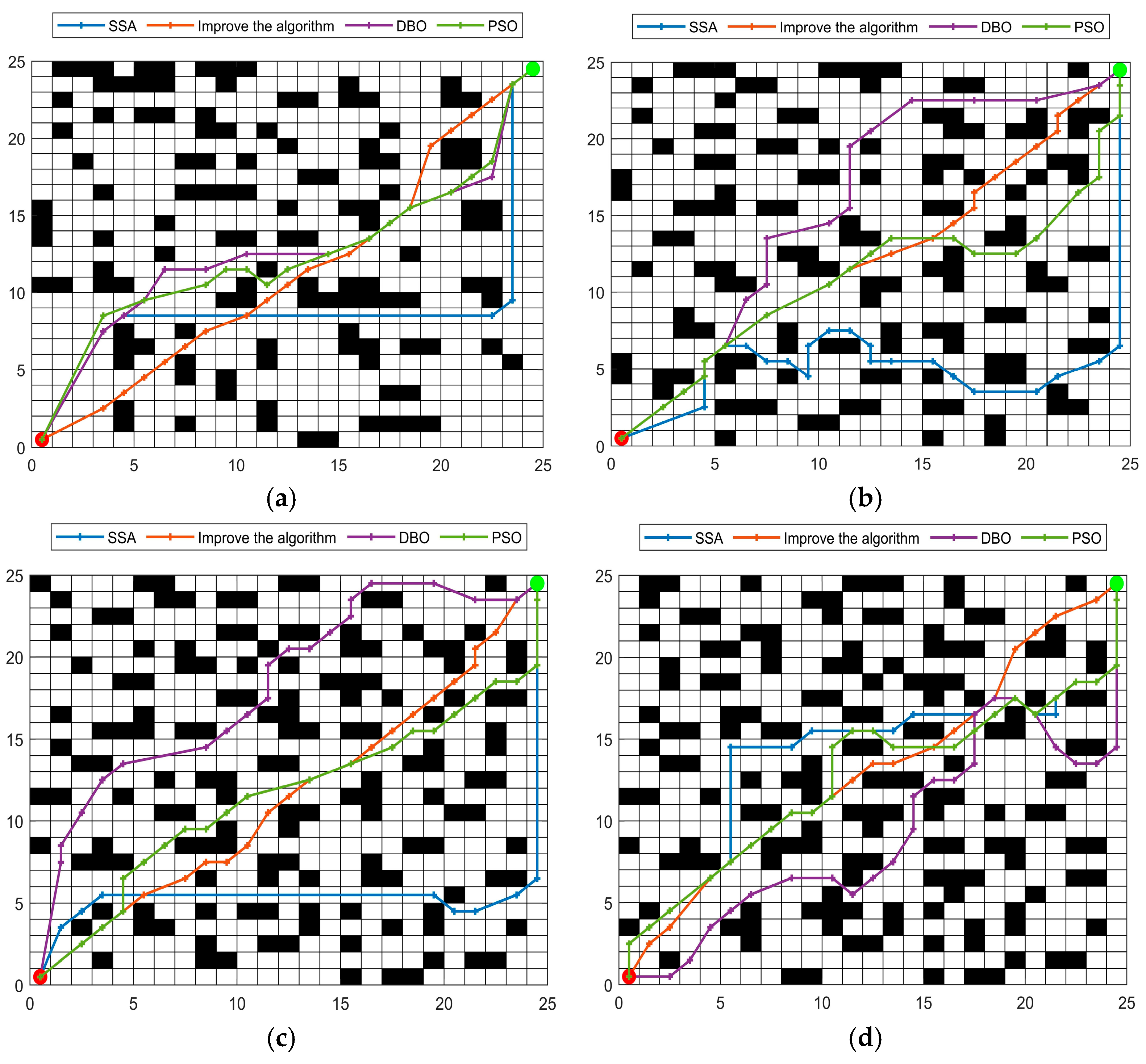
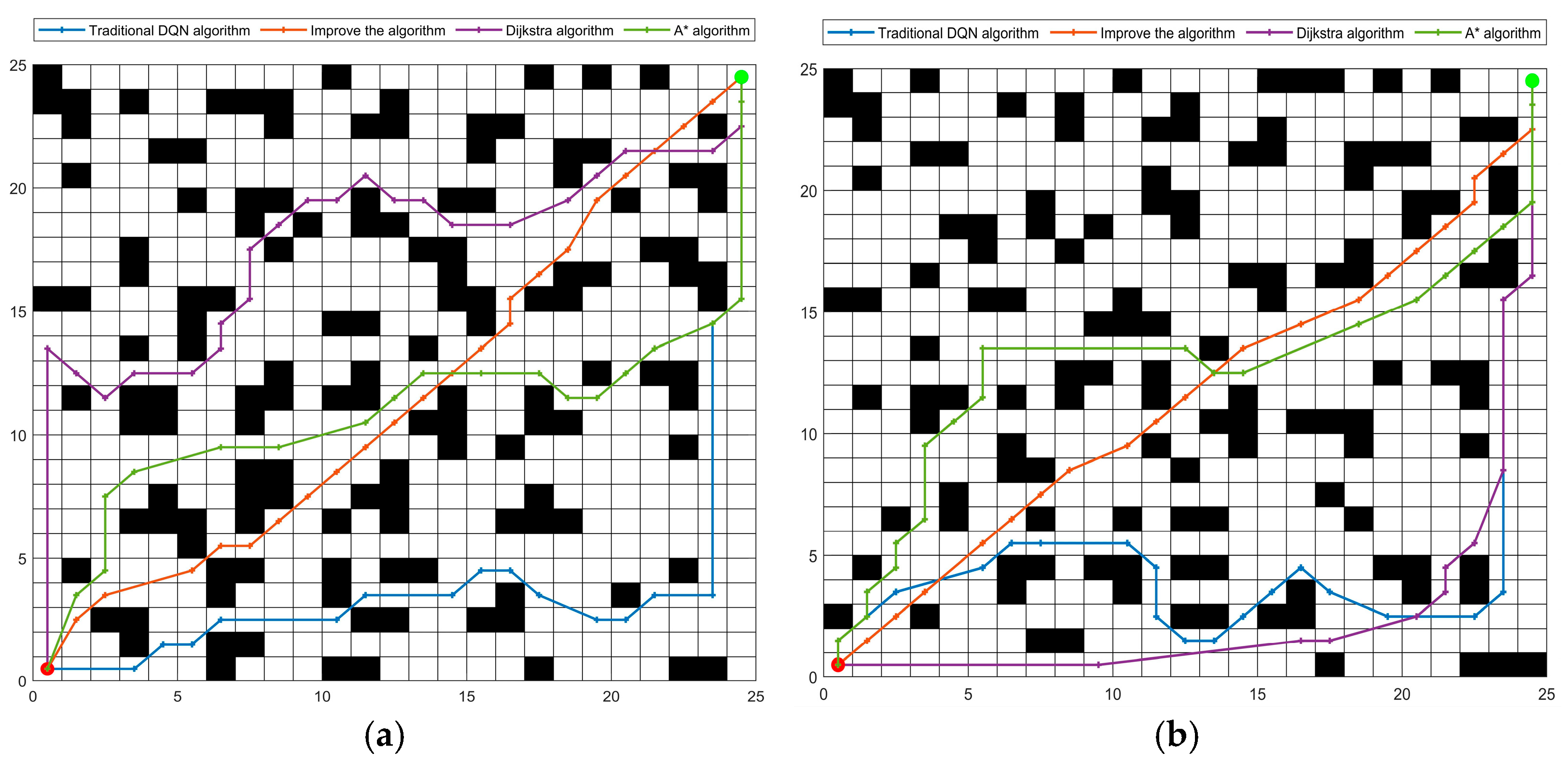
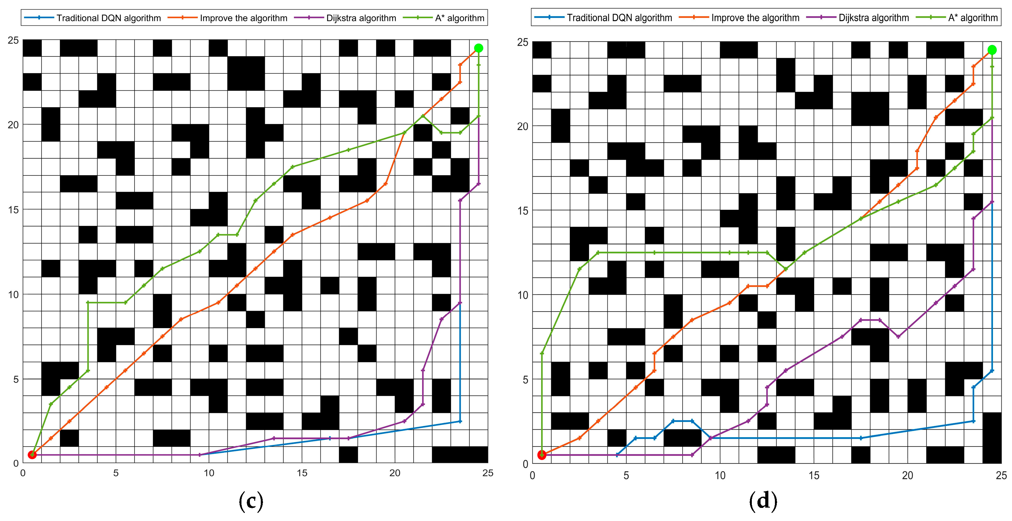
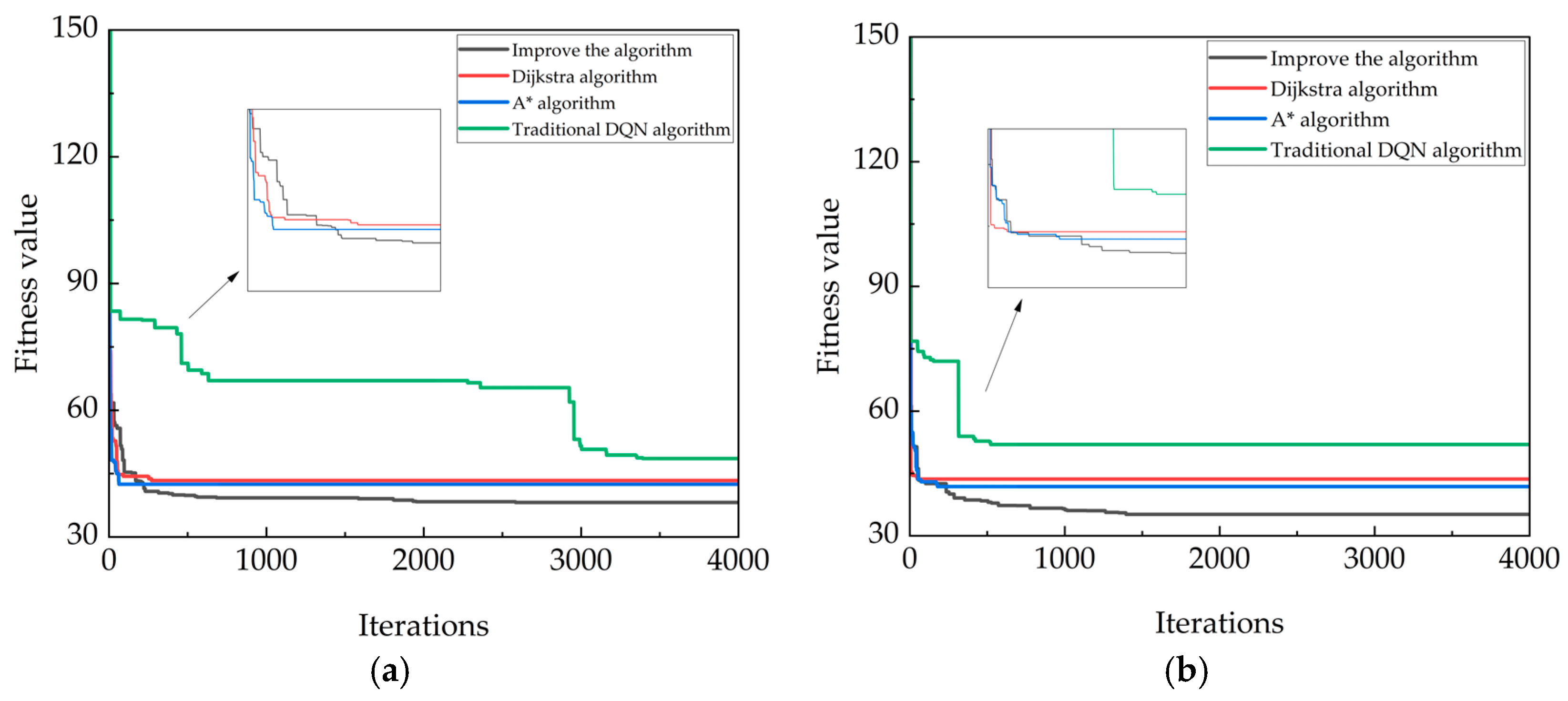
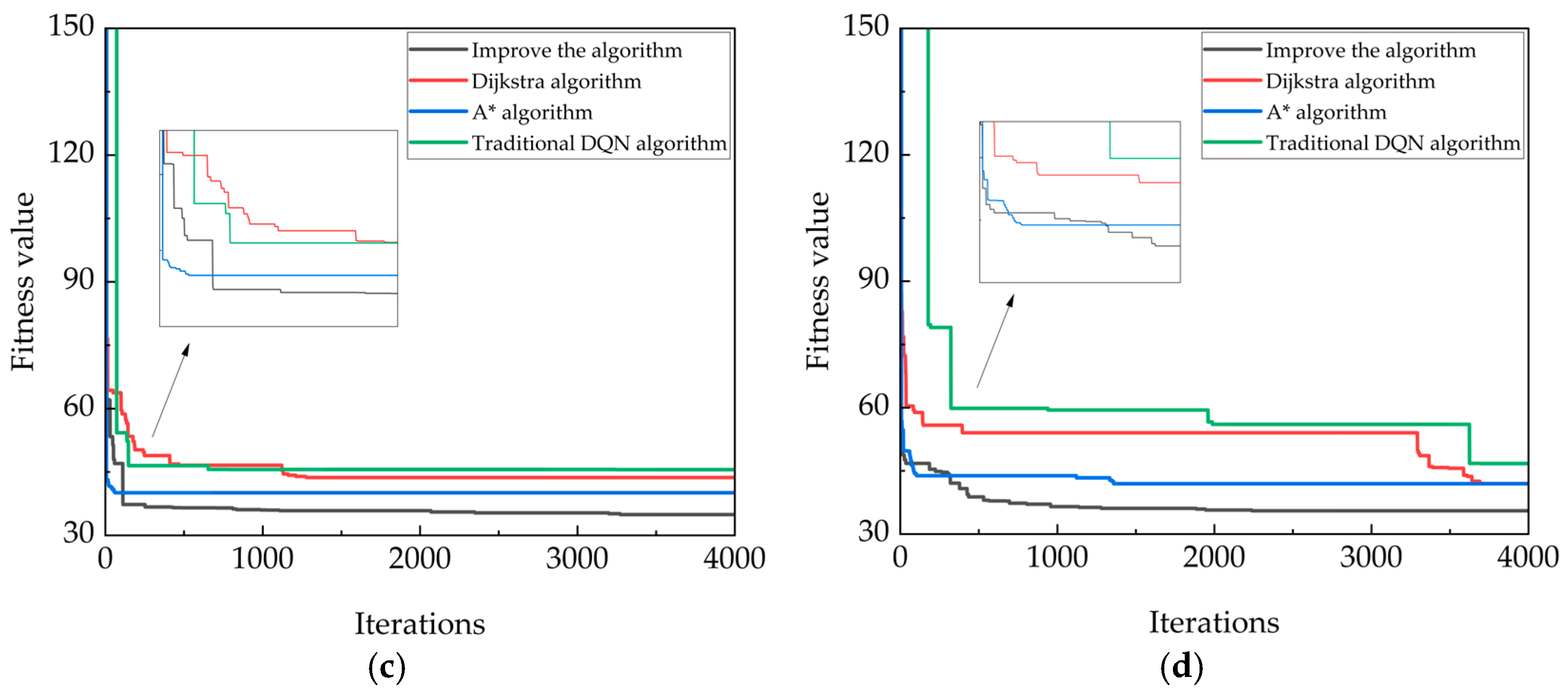
Through the construction of a grid map in Matlab (2022b), three maps of 20 × 20, 25 × 25, and 30 × 30 are constructed. In order to highlight the path planning ability and obstacle avoidance ability of the improved algorithm, it is compared with three current excellent algorithms: Particle Swarm Optimization (PSO), Sparrow Search Algorithm (SSA), and Dung Beetle Optimization (DBO). The above four algorithms are simulated and verified in the grid map. In order to be more convincing, the improved algorithm and the traditional algorithms (traditional double Q algorithm, A* algorithm, and Dijkstra algorithm) are simulated in a 25 × 25 environment to highlight the advantages of the improved algorithm.
In order to fully show the difference between the four algorithms and simulate a complex and random environment, four experiments were carried out in each size of the grid map, and the obstacles were placed randomly, which highlighted the advantages of the improved algorithm. As shown in Figure 6, Figure 7 and Figure 8, the simulation comparison between the improved algorithm and the traditional double Q algorithm, A* algorithm, and Dijkstra algorithm is shown in Figure 9.
Through the results of the above simulation experiments, it can be seen that the improved algorithm is superior to other algorithms in selecting the route to the end point. It is also better than other algorithms in the overall path planning, and can always select the best nearest route to reach the endpoint. The routes in three groups of grid maps of different sizes, and in three groups of twelve maps, show that the improved algorithm proposed in this paper performs better in complex environments.
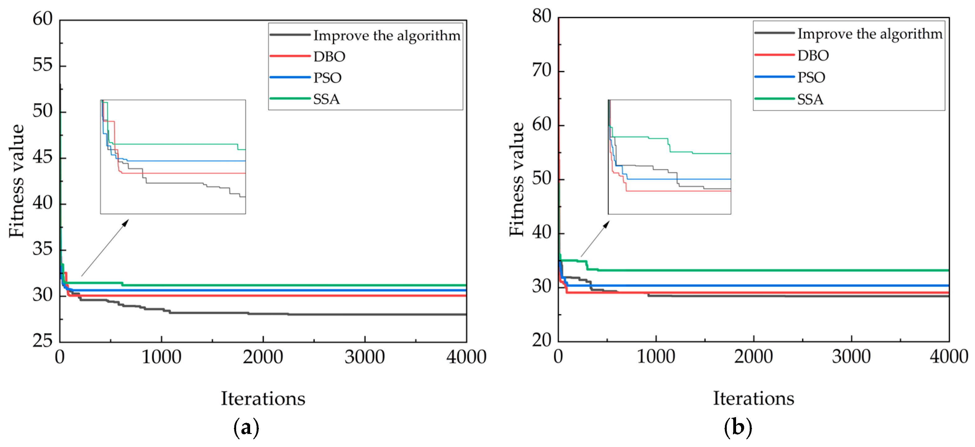
The simulation results show that the improved algorithm is superior to the other three algorithms in the overall path selection. In the chaotic environment of obstacles, a route with the shortest path can be selected. The improved algorithm only needs 35.9478 m to reach the end point in four experiments, while the traditional double Q algorithm, A* algorithm, and Dijkstra algorithm need 48.2068 m, 40.9287 m, and 43.17 m, respectively, which are improved by about 12%, 5.05%, and 7.2%, respectively. This shows that the improved algorithm proposed in this paper has better performance.
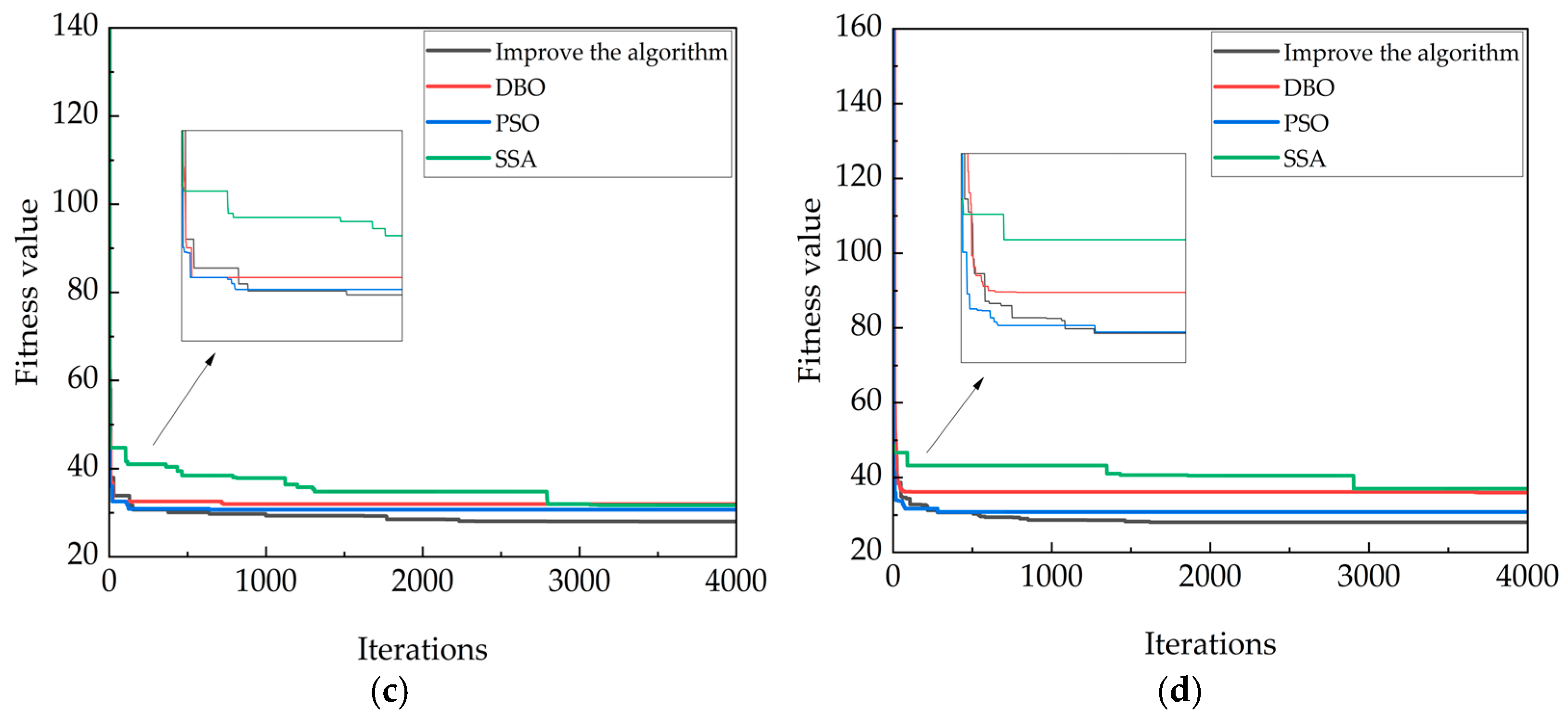
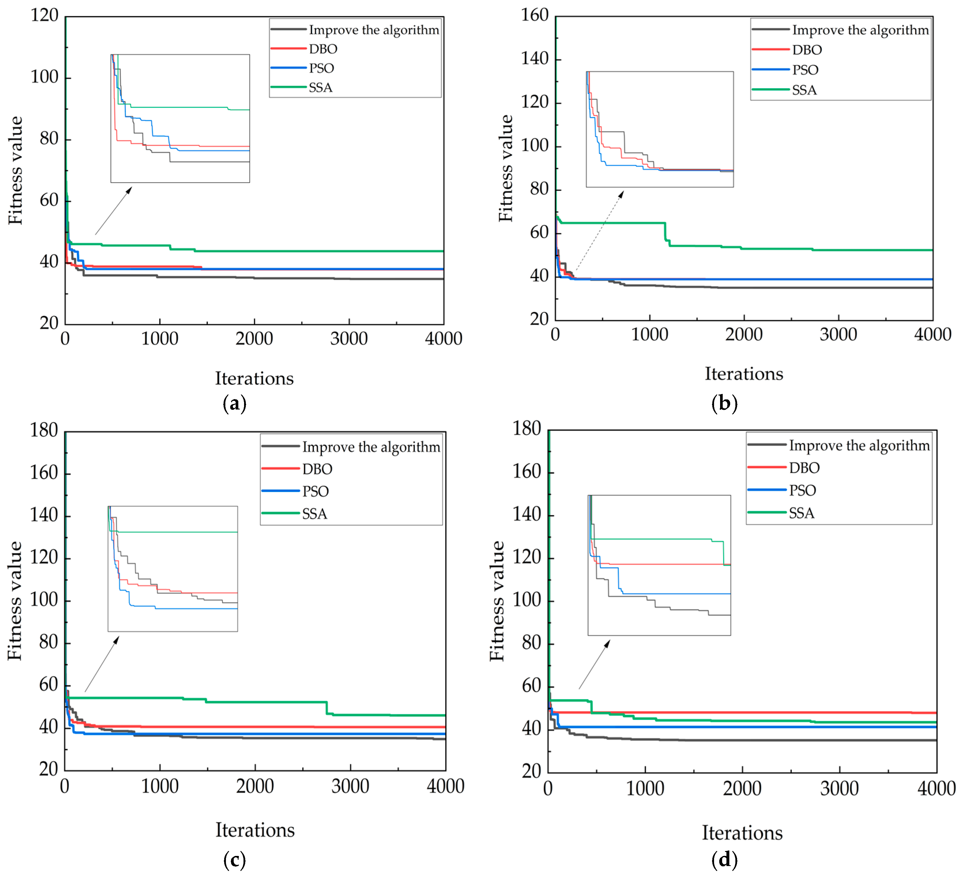
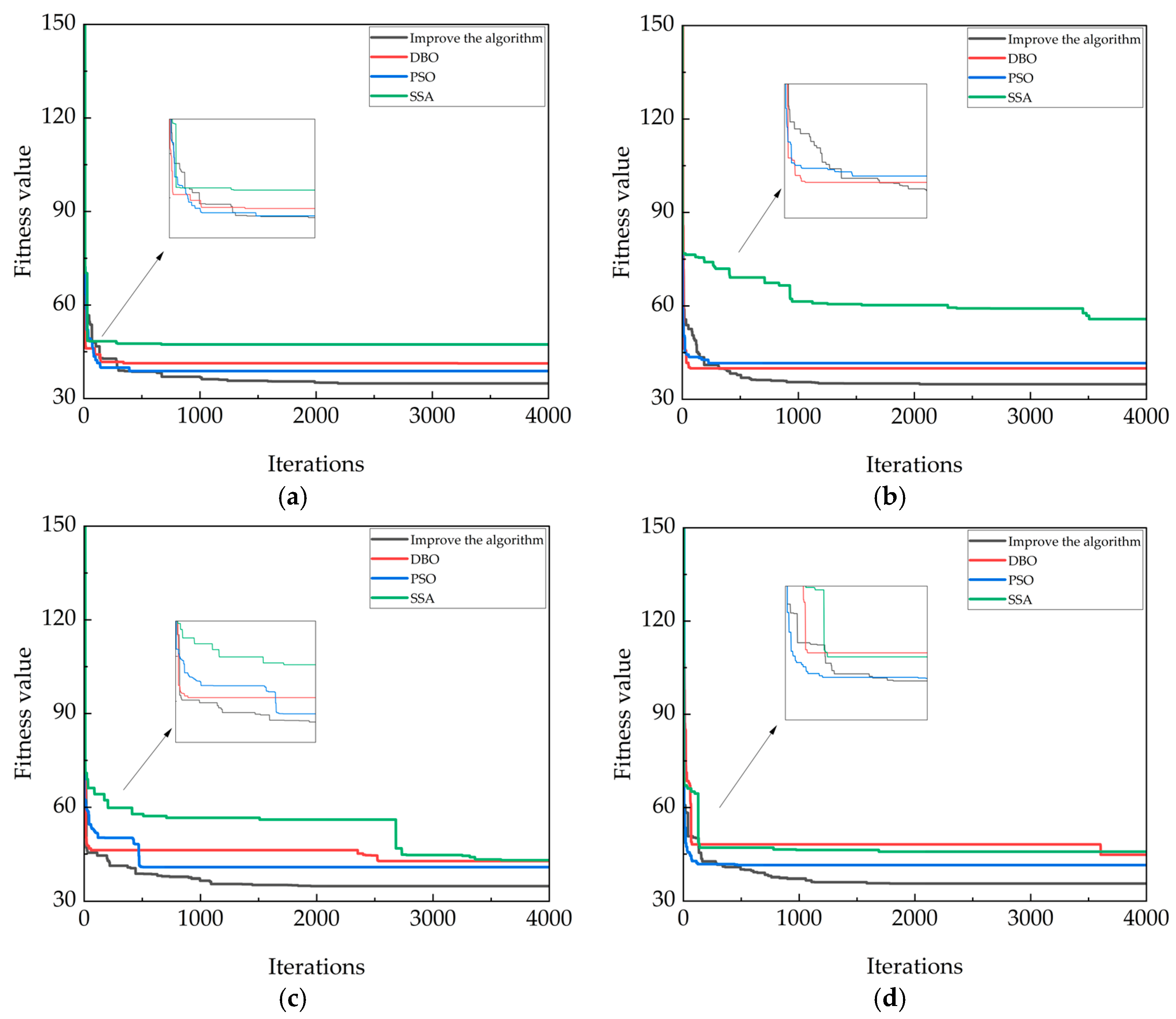
In order to show the advantages of the proposed algorithm more intuitively, the convergence curves of the four algorithms and other traditional algorithms in each simulation experiment are recorded, as shown in Figure 10, Figure 11, Figure 12 and Figure 13.
The convergence curves of the four algorithms in the above diagram show the shortcomings of the other three algorithms; that is, the convergence of the SSA algorithm is too late, and the DBO algorithm and the PSO algorithm exhibit instability, with convergence occurring too early or too late. In order to highlight the improved algorithm in the whole path planning process, it avoids premature convergence, stability, and other advantages.
In the whole process of road planning, the distance is also a reference quantity that can explain the problem. The following table shows the distance traveled by the four algorithms to the end point among the three grid maps, as shown in Table 2.
In order to show the difference of each algorithm in the distance more intuitively and clearly, the average distance of each algorithm in different-size maps is drawn into a histogram as shown in Figure 14, so as to highlight the advantages of the improved algorithm.
As shown in the above figure, in the 20 × 20 grid map, the improved algorithm reduces the distance by 6.53% compared with the SSA algorithm, and reduces the distance by 3.93% and 3.11% compared with the DBO algorithm and the PSO algorithm, respectively. In the 25 × 25 grid map, the improved algorithm reduces the distance by 11.42% compared with the SSA algorithm, and reduces the distance by 6.33% and 3.94%, respectively, compared with the DBO algorithm and the PSO algorithm. In the 30 × 30 grid map, the improved algorithm reduces the distance by 18.07% compared with the SSA algorithm, and by 7.91% and 5.57% compared with the DBO algorithm and the PSO algorithm, respectively. The above data show that the improved algorithm, combined with the curiosity module, performs better in environments with larger spaces and more obstacles.
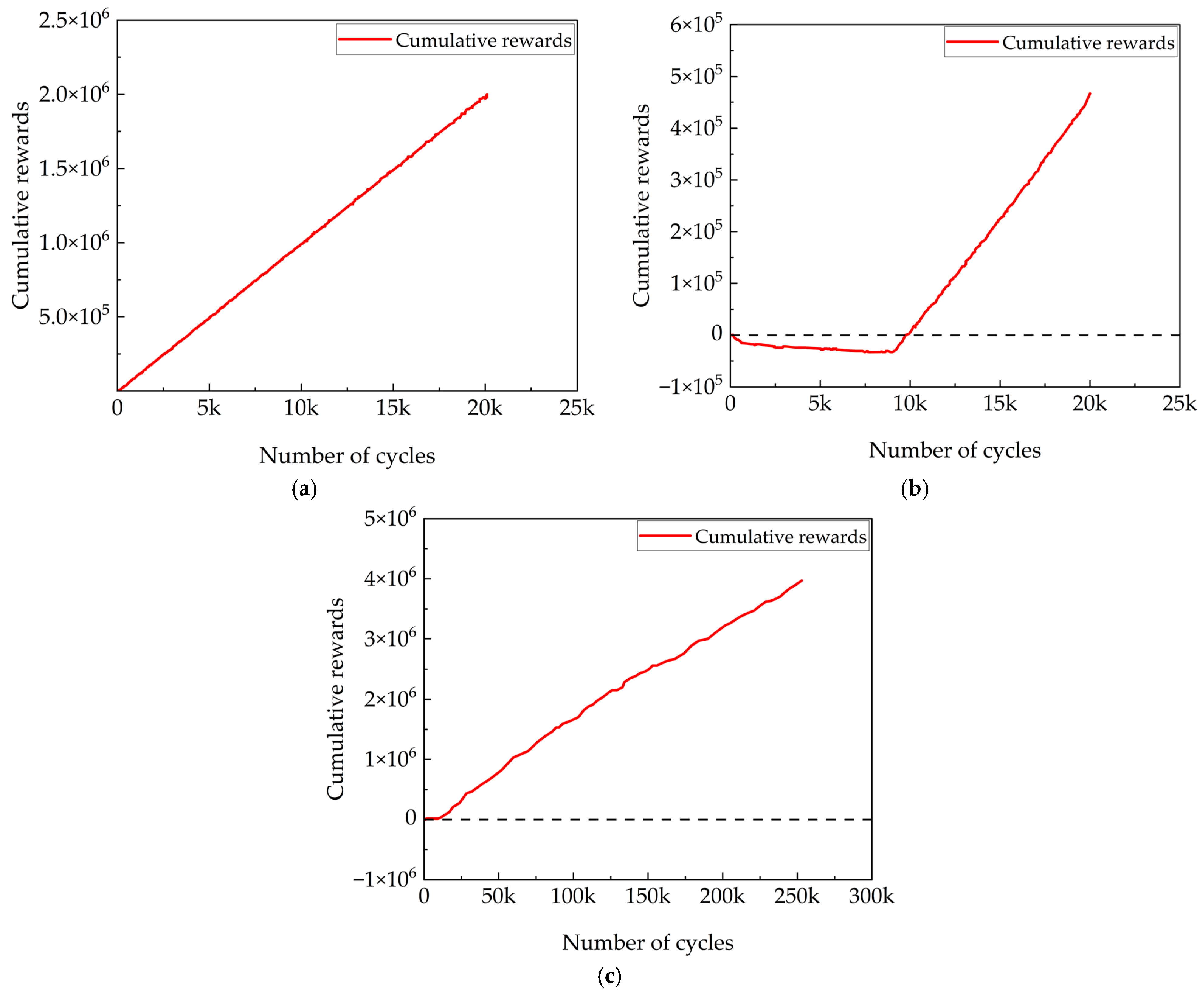
The improved algorithm with curiosity mechanism is stable in three grid environments and successfully finds the target path. Compared with the other three algorithms, it is more exploratory, and it is easier to explore the unknown area when encountering obstacles, so as to reach the target smoothly. In GMR training, set the reward to reach the end of 500, and hit the obstacle buckle to 50. In 20,000 cycles, the reward accumulated by the GMR is related to the number of times it reaches the end point, reflecting the performance of the improved algorithm. The following are the cumulative rewards in 20 × 20, 25 × 25, and 30 × 30 environments, as shown in Figure 15.
It can be seen from the diagram that the improved algorithm has a good performance in the whole road strength planning process. During the 20 × 20 cycle, the GMR accumulated a total reward of 1.9917 × 10⁶ and achieved good results. However, during the 25 × 25 cycle, the GMR accumulated a certain negative reward in the first half of the training, but because the negative reward was much lower than the positive reward obtained by reaching the target point during the whole training process, the final cumulative reward was still positive.
In the 30 × 30 map, the overall reward of the GMR is 4.427 × 10⁶, indicating that in a complex environment with many obstacles, the curiosity reward mechanism can effectively drive the GMR to explore more unknown areas and finally successfully reach the target area.
During the training process, although the performance of each cycle fluctuates, the overall performance is still excellent. This is due to the role of the curiosity mechanism. The GMR is more inclined to explore unknown areas. With the full exploration of the environment, the neural network estimates the value of the action more accurately.
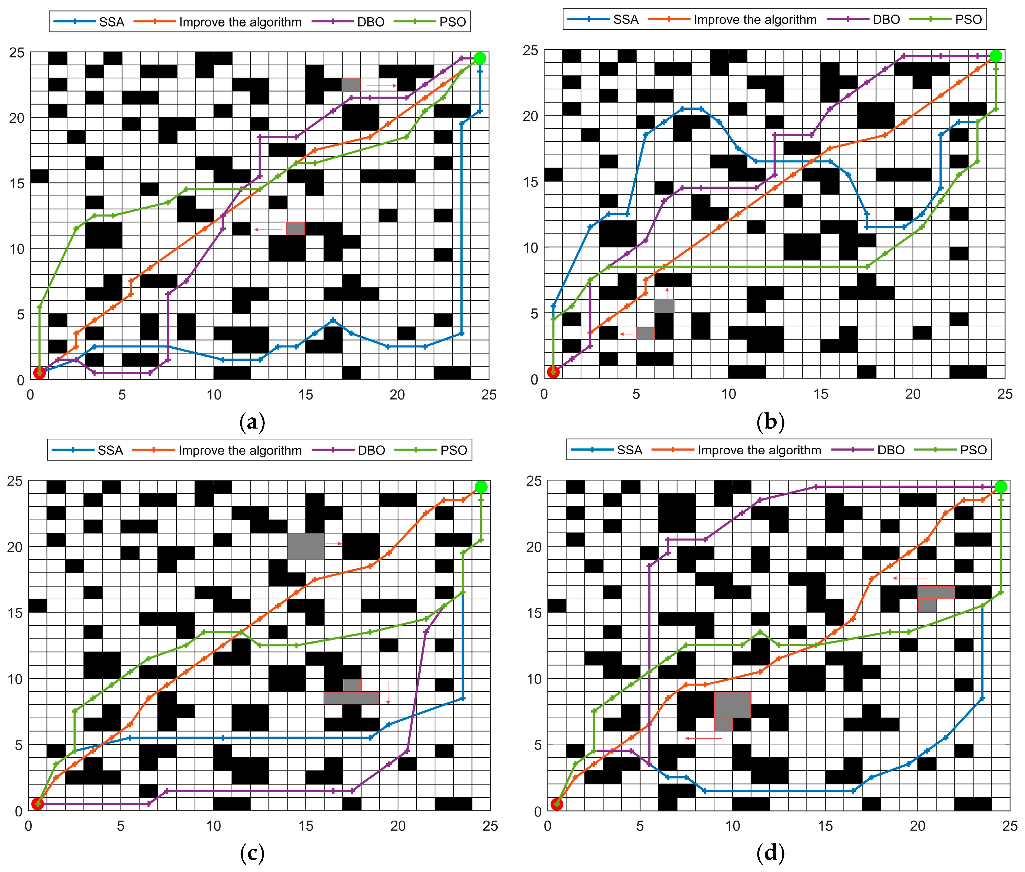
The above simulation experiments are all analyzed in the case of static obstacles. Next, through the combination of functions in Matlab (rand function, randperm (n), etc.), a random obstacle can be randomly moved in one of four directions—east, west, south, and north—to test the obstacle avoidance ability of the mobile robot driven by the algorithm. The initial position of the moving obstacle is marked as gray in the figure, the direction of movement is marked by the red arrow, and the black square indicated by the arrow is the place where the obstacle moves to. The simulation results are shown in Figure 16.
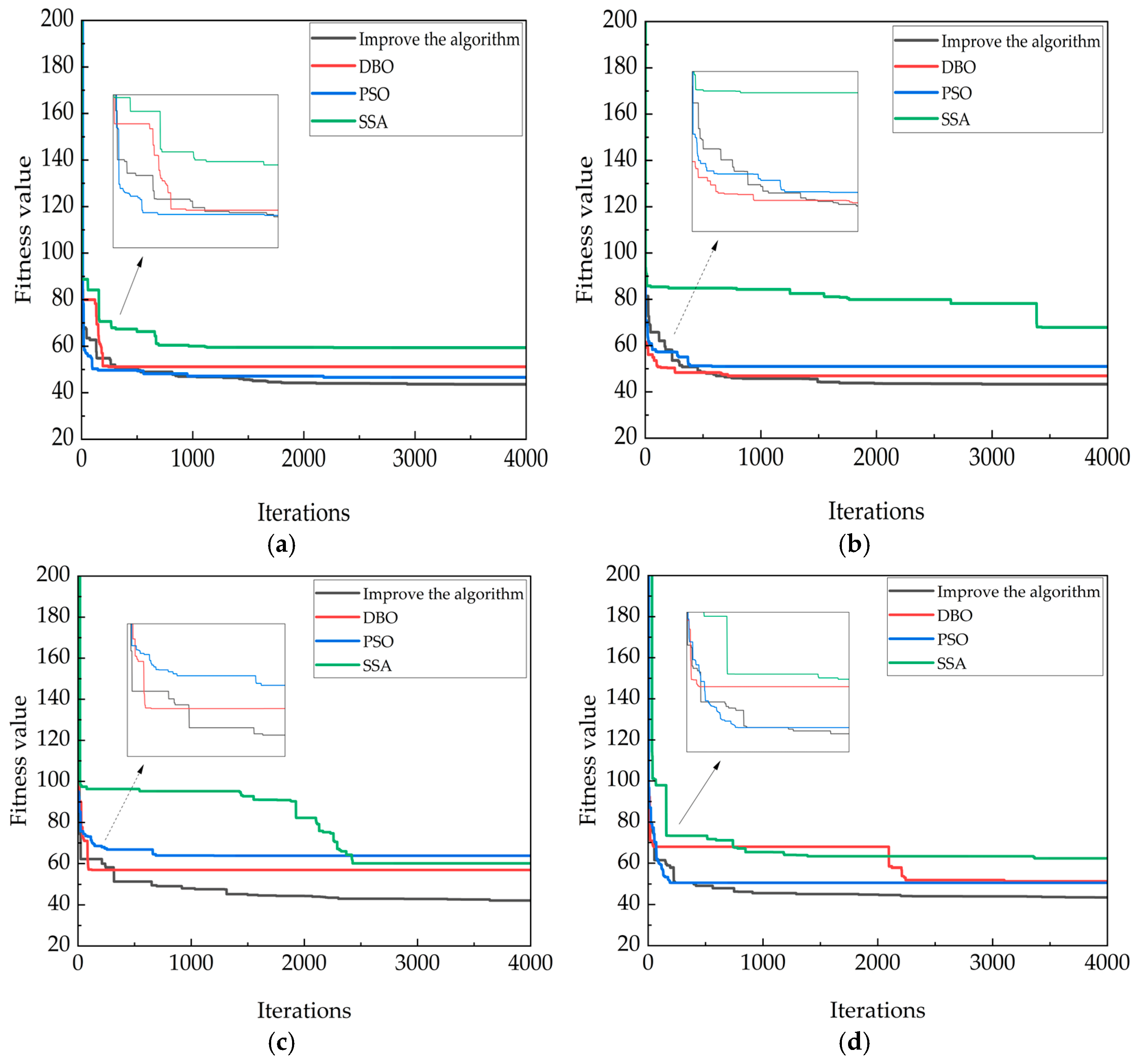
It can be seen from the diagram that even in the face of suddenly moving obstacles, the improved algorithm can still choose the most optimal path to pass. In Figure 17a, in the face of suddenly moving obstacles, the DBO algorithm chooses to circle an arc, which is not the optimal path. In Figure 17b–d, in the face of moving obstacles, the improved algorithm can avoid and select an optimal path in time to reach the end point. In order to illustrate the differences between the four algorithms more intuitively, the convergence curve is shown in Figure 17.
The convergence curve above shows that under the environmental conditions of movable obstacles, the DBO algorithm, PSO algorithm, and SSA algorithm all have the disadvantages of improper convergence time and vulnerability to noise and other disturbances, which highlights the advantages of the improved algorithm. Compared with DBO, PSO, and SSA algorithms, the improved algorithm increases the moving distance by 7.02%, 6.02%, and 9.7%, respectively, showing that the improved algorithm can still choose the optimal path in a complex, unknown environment.
Finally, the GMR driven by the improved algorithm can choose the shortest path to reach the end point, and is superior to PSO, SSA, and DBO algorithms in the process of overall road strength planning. Whether in a static obstacle environment or a mobile obstacle environment, the GMR driven by the improved algorithm can select the shortest path to the end point, and is superior to the PSO, SSA, and DBO algorithms in the overall path planning process. Moreover, the performance of the improved algorithm in the simulation experiment is better than the traditional DQN algorithm, A* algorithm, and Dijkstra algorithm.

5. Conclusions

Under the interference of noise conditions, the navigation accuracy and stability of the traditional algorithm are greatly reduced, and there is a risk of overestimation and bootstrapping. In order to solve the above problems, a curiosity-driven algorithm based on self-supervised prediction is proposed:
(1)
After introducing the curiosity mechanism and training, the GMR obtains a higher positive reward. By using the internal reward to guide GMR exploration, the reward setting is optimized, priority experience playback is added to improve the training efficiency, and the navigation accuracy and stability in the complex environment are improved.
(2)
The simulation experiment of the grid environment shows that the exploration mechanism of reinforcement learning is improved after adding curiosity. It not only successfully explores the unknown environment and successfully reaches the end of the environment model, but also fully illustrates that the GMR solves the convergence problem of double Q-learning path planning in a complex environment after combining a curiosity mechanism. The GMR successfully finds the shortest path to reach the end point in the environment and obtains higher positive rewards. In the 20 × 20, 25 × 25, and 30 × 30 grid maps, the path distance of the improved algorithm is shorter than that of the SSA, DBO, and PSO algorithms, and the maximum shortening ranges are 6.53%, 11.42%, and 18.07%, respectively. In the 25 × 25 environment, the performance of the improved algorithm is better than that of the traditional DQN algorithm, A* algorithm, and Dijkstra algorithm, and the maximum shortening is 12%, 5.05%, and 7.2%, respectively. The results show that the improved algorithm, combined with the curiosity module, performs better in a larger environment with more obstacles. In different environments, although the overall reward fluctuates, it is still positive in the end.
(3)
Combined with the above simulation experiments and data, it is shown that the algorithm proposed in this paper has stronger noise suppression ability, stronger stability, and higher accuracy than conventional PSO, SSA, DBO, Dijkstra, A * , and other algorithms, which are conducive to the exploration of GMRs in unknown environments.
To evaluate the adaptability of the improved double Q-learning algorithm in larger environments, we conducted experimental comparisons under different scales of state spaces. As the complexity of the environment increased (such as larger map sizes and higher state dimensions), the traditional double Q algorithm showed significant declines in convergence speed and policy performance, manifested as an increase in training steps and a decrease in average rewards. However, by introducing a curiosity mechanism and combining it with a competitive network, our algorithm effectively mitigated the impact of state dimensions, enabling stable updates of the double Q value function in high-dimensional environments and maintaining high policy performance. In terms of memory overhead, our algorithm uses a shared structure to update two sets of Q values, effectively reducing the consumption of redundant computing resources. Overall, the experimental results in different scale environments indicate that the improved double Q algorithm has good scalability and is suitable for a wider range of practical problem scenarios.
Looking forward to the future, with continuous breakthroughs in the fields of intelligent algorithms, sensing technology, and energy management, ground mobile robots will become more intelligent, flexible, and stable, allowing them to complete tasks independently in more complex environments. Especially when performing tasks in unfamiliar environments, the success rate and completion efficiency will be higher. For example, during mountain fires or earthquakes, search and rescue personnel often cannot reach areas with harsh environmental conditions and high risk factors, while unmanned robots will be competent enough for environmental investigation tasks. The implementation of algorithms with high efficiency and a success rate can improve work efficiency and protect search and rescue operations. As an important part of modern intelligent technology, they have broad development prospects in the future. With the continuous progress of artificial intelligence, sensor technology, automatic control, and communication technology, ground mobile robots will be used more and more in all walks of life to promote the intelligent transformation of society. Collaboration between humans and robots will become increasingly close, and robots will become a powerful partner in our lives, work, and exploration of the unknown world.

Author Contributions

Conceptualization, J.Z., X.R. (Xiaowei Ren) and L.F.; Data Management, N.W. and Y.Z. (Yu Zhang); Investigation, J.F., Y.Z. (Yu Zhang) and X.R. (Xu Ren); Methodology, J.Z., L.F., L.N., and N.W.; Project Management, J.Z.; Software, J.Z., J.W. and J.F.; Supervision, Y.Z. (Ya Zhang); Verification, X.H., L.N., and J.Z.; Writing—Original manuscript, J.Z. and X.R.; Writing—Review and Editing, Y.Z. (Ya Zhang). All authors have read and agreed to the published version of the manuscript.

Funding

This research was funded by the Shanxi Provincial Postgraduate Scientific Research Innovation Project under Grant 2024SJ247.

Institutional Review Board Statement

Not applicable.

Informed Consent Statement

Not applicable.

Data Availability Statement

Data are contained within the article.

Conflicts of Interest

The authors declare no conflicts of interest.

Abbreviations

The abbreviations and their explanations that appear in this article are as follows:
SSASparrow Search Algorithm
DBODung Beetle Optimization
PSOParticle Swarm Optimization
GMRGround mobile robot
RRTRapidly-exploring Random Trees
DQNDeep Q-network
ICMIntrinsic curiosity module
UCBUpper confidence bound

References

  1. Wang, H.; Liu, J.; Dong, H.; Shao, Z. A Survey of the Multi-Sensor Fusion Object Detection Task in Autonomous Driving. Sensors 2025, 25, 2794. [Google Scholar] [CrossRef] [PubMed]
  2. Carberry, S. Land Mass: Ground Robot Swarm Tech Crawling Along. Natl. Def. 2024, 109. [Google Scholar]
  3. Ou, Y.; Cai, Y.; Sun, Y.; Qin, T. Correction: Ou et al. Autonomous Navigation by Mobile Robot with Sensor Fusion Based on Deep Reinforcement Learning. Sensors 2024, 24, 3895. [Google Scholar] [CrossRef]
  4. Yan, W.; Xu, X.; Rodić, A.; Petrovich, P.B. FRRT*-Connect: A Bidirectional Sampling-Based Path Planner with Potential Field Guidance for Complex Obstacle Environments. Sensors 2025, 25, 2761. [Google Scholar] [CrossRef]
  5. Wolf, Y.; Levy, E.; Rotbart, M. Ground Robot Drive System: US15450445. US20170174278A1, 20 March 2025. [Google Scholar]
  6. Hong, F.; Zhao, Y.; Ji, W.; Hao, J.; Fang, F.; Liu, J. A dynamic migration route planning optimization strategy based on real-time energy state observation considering flexibility and energy efficiency of thermal power unit. Appl. Energy 2025, 377, 124575. [Google Scholar] [CrossRef]
  7. Cao, M.; Xu, X.; Cao, K.; Xie, L. System identification and control of the ground operation mode of a hybrid aerial–ground robot. Control Theory Technol. 2023, 21, 458–468. [Google Scholar] [CrossRef]
  8. Parkhomenko, V.; Medvedev, M. Nerual Network System For Ground Robot Path Planning and Obstacle Avoidance. In Proceedings of the 2021 7th International Conference on Mechatronics and Robotics Engineering (ICMRE), Budapest, Hungary, 3–5 February 2021. [Google Scholar] [CrossRef]
  9. Tavares, A.J.A., Jr.; Oliveira, N.M.F. A Novel Approach for Kalman Filter Tuning for Direct and Indirect Inertial Navigation System/Global Navigation Satellite System Integration. Sensors 2024, 24, 7331. [Google Scholar] [CrossRef]
  10. Bansal, T.; Anand, S. Probabilistic Roadmap Generation for Autonomous Robot Path Planning in Dynamic Environments. In International Conference on Mechanical and Energy Technologies; Springer: Singapore, 2024. [Google Scholar] [CrossRef]
  11. Altun, G.; Aydin, L. Optimizing Unmanned Vehicle Navigation: A Hybrid PSO-GWO Algorithm for Efficient Route Planning. Firat Univ. J. Exp. Comput. Eng. FUJECE 2025, 4, 100–114. [Google Scholar] [CrossRef]
  12. Xue, Q.; Zheng, S.-T.; Han, X.; Jiang, R. A two-level framework for dynamic route planning and trajectory optimization of connected and automated vehicles in road networks. Phys. A Stat. Mech. Its Appl. 2025, 668, 130552. [Google Scholar] [CrossRef]
  13. Chen, M.Z.; Zhu, D.Q. Optimal Time-Consuming Path Planning for Autonomous Underwater Vehicles Based on a Dynamic Neural Network Model in Ocean Current Environments. IEEE Trans. Veh. Technol. 2020, 69, 14401–14412. [Google Scholar] [CrossRef]
  14. AbuJabal, N.; Rabie, T.; Baziyad, M.; Kamel, I.; Almazrouei, K. Path Planning Techniques for Real-Time Multi-Robot Systems: A Systematic Review. Electronics 2024, 13, 2239. [Google Scholar] [CrossRef]
  15. Yang, Z.; Zhuang, Y.; Chen, Y. Path planning of a building robot based on BIM and an improved RRT algorithm. Exp. Technol. Manag. 2024, 41, 31–42. [Google Scholar] [CrossRef]
  16. Sahoo, B.; Das, D.; Pujhari, K.C.; Vikas. Optimization of route planning for the mobile robot using a hybrid Neuro-IWO technique. Int. J. Inf. Technol. 2025, 17, 1431–1439. [Google Scholar] [CrossRef]
  17. Fan, J.; Zhang, X.; Zou, Y.; Li, Y.; Liu, Y.; Sun, W. Improving policy training for autonomous driving through randomized ensembled double Q-learning with Transformer encoder feature evaluation. Appl. Soft Comput. 2024, 167, 112386. [Google Scholar] [CrossRef]
  18. Liao, S.; Xiao, W.; Wang, Y. Optimization of route planning based on active towed array sonar for underwater search and rescue. Ocean. Eng. 2025, 330, 121249. [Google Scholar] [CrossRef]
  19. Moras, J. Continuous Online Semantic Implicit Representation for Autonomous Ground Robot Navigation in Unstructured Environments. Robotics 2024, 13, 108. [Google Scholar] [CrossRef]
  20. Pan, Y.; Li, L.; Qin, J.; Chen, J.; Gardoni, P. Unmanned aerial vehicle–human collaboration route planning for intelligent infrastructure inspection. Comput.-Aided Civ. Infrastruct. Eng. 2024, 39, 2074–2104. [Google Scholar] [CrossRef]
  21. Tai, L. Sensorimotor Learning for Ground Robot Navigation. Ph.D. Thesis, The Hong Kong University of Science and Technology, Hong Kong, China, 2019. [Google Scholar] [CrossRef]
  22. Saga, R.; Kozono, R.; Tsurumi, Y.; Nihei, Y. Deep-reinforcement learning-based route planning with obstacle avoidance for autonomous vessels. Artif. Life Robot. 2024, 29, 136–144. [Google Scholar] [CrossRef]
  23. Yin, Y.; Zhang, L.; Shi, X.; Wang, Y.; Peng, J.; Zou, J. Improved Double Deep Q Network Algorithm Based on Average Q-Value Estimation and Reward Redistribution for Robot Path Planning. Comput. Mater. Contin. 2024, 81, 2769–2790. [Google Scholar] [CrossRef]
  24. Puvaneswari, G. An Efficient Double Deep Q Learning Network-Based Soft Faults Detection and Localization in Analog Circuits. J. Circuits Syst. Comput. 2024, 33, 2450230. [Google Scholar] [CrossRef]
  25. Hewing, L.; Kabzan, J.; Zeilinger, M.N. Cautious Model Predictive Control Using Gaussian Process Regression. IEEE Trans. Control Syst. Technol. 2020, 28, 2736–2743. [Google Scholar] [CrossRef]
  26. Saccani, D.; Cecchin, L.; Fagiano, L. Multitrajectory Model Predictive Control for Safe UAV Navigation in an Unknown Environment. IEEE Trans. Control Syst. Technol. 2023, 31, 1982–1997. [Google Scholar] [CrossRef]
  27. Fossen, T.I. An Adaptive Line-of-Sight (ALOS) Guidance Law for Path Following of Aircraft and Marine Craft. IEEE Trans. Control Syst. Technol. 2023, 31, 2887–2894. [Google Scholar] [CrossRef]
  28. Fan, Y.; Dong, H.; Zhao, X.; Denissenko, P. Path-Following Control of Unmanned Underwater Vehicle Based on an Improved TD3 Deep Reinforcement Learning. IEEE Trans. Control Syst. Technol. 2024, 32, 1904–1919. [Google Scholar] [CrossRef]
  29. De Lellis, F.; Coraggio, M.; Russo, G.; Musolesi, M.; di Bernardo, M. Guaranteeing Control Requirements via Reward Shaping in Reinforcement Learning. IEEE Trans. Control Syst. Technol. 2024, 32, 2102–2113. [Google Scholar] [CrossRef]
  30. Sharifi, M.; Azimi, V.; Mushahwar, V.K.; Tavakoli, M. Impedance Learning-Based Adaptive Control for Human–Robot Interaction. IEEE Trans. Control Syst. Technol. 2022, 30, 1345–1358. [Google Scholar] [CrossRef]
  31. Bai, H.; Gao, W.; Ma, H.; Ding, P.; Wang, G.; Xu, W.; Wang, W.; Du, Z. A study of robotic search strategy for multi-radiation sources in unknown environments. Robot. Auton. Syst. 2023, 169, 18. [Google Scholar] [CrossRef]
  32. Feng, A.; Xie, Y.; Sun, Y.; Wang, X.; Jiang, B.; Xiao, J. Efficient Autonomous Exploration and Mapping in Unknown Environments. Sensors 2023, 23, 4766. [Google Scholar] [CrossRef]
  33. Bellemare, M.G.; Srinivasan, S.; Ostrovski, G.; Schaul, T.; Saxton, D.; Munos, R. Unifying Count-Based Exploration and Intrinsic Motivation. arXiv 2016, arXiv:1606.01868. [Google Scholar] [CrossRef]
  34. Tang, H.; Houthooft, R.; Foote, D.; Stooke, A.; Chen, X.; Duan, Y.; Schulman, J.; De Turck, F.; Abbeel, P. #Exploration: A study of count-based exploration for deep reinforcement learning. In Proceedings of the 31st International Conference on Neural Information Processing Systems, Long Beach, CA, USA, 4–9 December 2017. [Google Scholar]
  35. Stadie, B.C.; Levine, S.; Abbeel, P. Incentivizing exploration in reinforcement learning with deep predictive models. arXiv 2015, arXiv:1507.00814. [Google Scholar] [CrossRef]
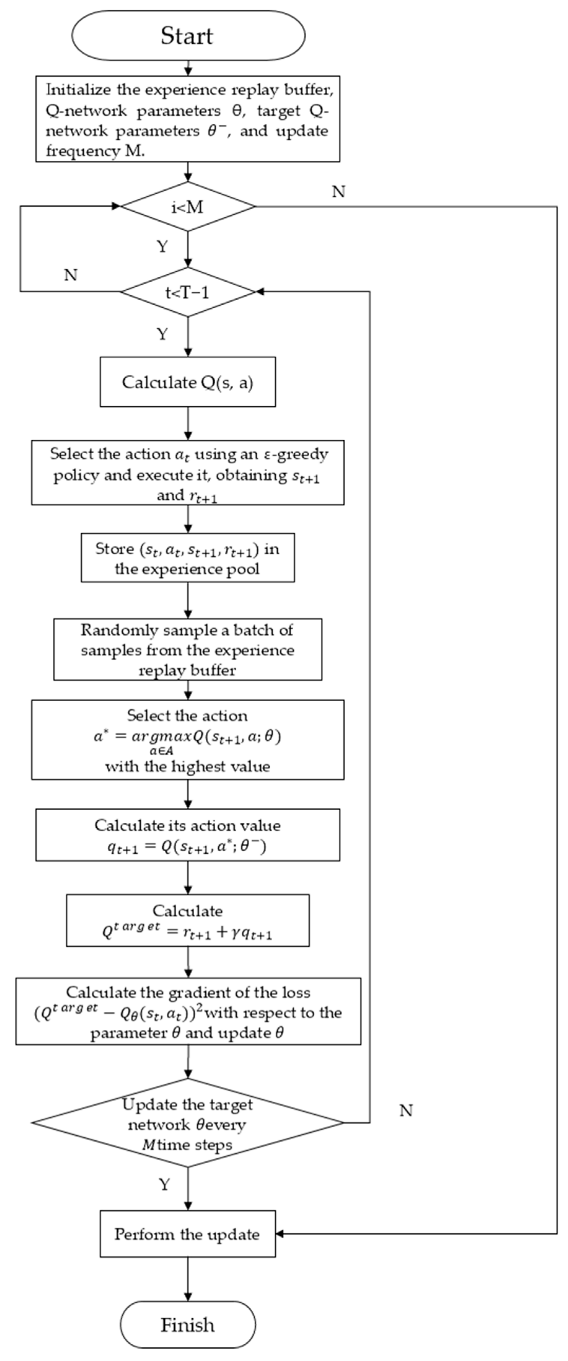
Figure 1. Double Q-learning.
Symmetry 17 01530 g001
Figure 2. Competitive Network.
Symmetry 17 01530 g002
Figure 3. Forward model.
Symmetry 17 01530 g003
Figure 4. Combined with a flow chart.
Symmetry 17 01530 g004
Figure 5. Training process.
Symmetry 17 01530 g005
Figure 6. Simulation experiments of four algorithms in 20 × 20 environment. (a) The simulation result diagram in the first type of map; (b) The simulation result diagram in the second type of map; (c) The simulation result diagram in the third type of map; (d) The simulation result diagram in the fourth type of map.
Symmetry 17 01530 g006aSymmetry 17 01530 g006b
Figure 7. Simulation experiments of four algorithms in 25 × 25 environment. (a) The simulation result diagram in the first type of map; (b) The simulation result diagram in the second type of map; (c) The simulation result diagram in the third type of map; (d) The simulation result diagram in the fourth type of map.
Symmetry 17 01530 g007
Figure 8. Simulation experiments of four algorithms in 30 × 30 environment. (a) The simulation result diagram in the first type of map; (b) The simulation result diagram in the second type of map; (c) The simulation result diagram in the third type of map; (d) The simulation result diagram in the fourth type of map.
Symmetry 17 01530 g008
Figure 9. The simulation comparison between the improved algorithm and the traditional double Q algorithm, A* algorithm, and Dijkstra algorithm. (a) The simulation result diagram in the first type of map; (b) The simulation result diagram in the second type of map; (c) The simulation result diagram in the third type of map; (d) The simulation result diagram in the fourth type of map.
Symmetry 17 01530 g009aSymmetry 17 01530 g009b
Figure 10. The convergence curve of the simulation experiment in 20 × 20 environment. (a) The convergence map in the first type of map; (b) The convergence map in the second type of map; (c) The convergence map in the third type of map; (d) The convergence map in the fourth type of map.
Symmetry 17 01530 g010aSymmetry 17 01530 g010b
Figure 11. The convergence curve of the simulation experiment in 25 × 25 environment. (a) The convergence map in the first type of map; (b) The convergence map in the second type of map; (c) The convergence map in the third type of map; (d) The convergence map in the fourth type of map.
Symmetry 17 01530 g011
Figure 12. The convergence curve of the simulation experiment in 30 × 30 environment. (a) The convergence map in the first type of map; (b) The convergence map in the second type of map; (c) The convergence map in the third type of map; (d) The convergence map in the fourth type of map.
Symmetry 17 01530 g012
Figure 13. In the 25 × 25 environment, the improved algorithm and four traditional algorithms simulate the convergence curve of the simulation experiment. (a) The convergence map in the first type of map; (b) The convergence map in the second type of map; (c) The convergence map in the third type of map; (d) The convergence map in the fourth type of map.
Symmetry 17 01530 g013aSymmetry 17 01530 g013b
Figure 14. The average distance of four algorithms in three grid maps: (a) The average distance of different algorithms in a 20 × 20 map; (b) the average distance of different algorithms in a 25 × 25 map; (c) the average distance of different algorithms in a 30 × 30 map.
Symmetry 17 01530 g014
Figure 15. Cumulative reward: (a) 20 × 20 cumulative reward; (b) 25 × 25 cumulative reward; (c) 30 × 30 cumulative reward.
Symmetry 17 01530 g015
Figure 16. Simulation of four algorithms in a 25 × 25 environment. (a) The simulation result diagram in the first type of map; (b) The simulation result diagram in the second type of map; (c) The simulation result diagram in the third type of map; (d) The simulation result diagram in the fourth type of map.
Symmetry 17 01530 g016
Figure 17. Convergence curves of four algorithms in a moving obstacle environment. (a) The convergence map in the first type of map; (b) The convergence map in the second type of map; (c) The convergence map in the third type of map; (d) The convergence map in the fourth type of map.
Symmetry 17 01530 g017
Table 1. Experimental parameter settings.
ParameterImplicationNumerical Value
εsearch strategy0.9
βProportion of forward loss0.8
αlearning rate0.0001
γdiscount factor0.9
i_scaleInternal reward ratio coefficient0.6
e_scaleExternal Rewards Proportion Coefficient0.4
TOTALTotal number of training15,000
MEMORY_CAPACITYExperience pool2000
TARGET_REPLACE_ITERTarget network parameter update interval200
BATCH_SIZENumber of one training64
Table 2. The driving distance of the four algorithms in the three maps.
Map SizeAlgorithm
SSAImprove the AlgorithmDBOPSO
20 × 2035.056426.347829.551431.4204
33.207428.426829.077830.3883
31.712128.019231.964130.6962
37.022628.093236.006730.8259
25 × 2543.858434.828237.949938.0633
52.436135.119339.043239.0101
46.055234.985940.630337.4334
43.556335.275247.914841.4558
30 × 3059.384843.627651.151646.6471
61.190842.465651.801250.1706
66.649343.740550.611648.1259
62.333843.458151.334650.5918
Disclaimer/Publisher’s Note: The statements, opinions and data contained in all publications are solely those of the individual author(s) and contributor(s) and not of MDPI and/or the editor(s). MDPI and/or the editor(s) disclaim responsibility for any injury to people or property resulting from any ideas, methods, instructions or products referred to in the content.