Quadratic Control Model for Shuttle Dispatching in Automated Overhead Rail Systems

Abstract

Automated Overhead Rail Systems (AORs) have a key role in warehouse and in-house industry, as well as in the modern hospital, where efficient shuttle dispatching directly impacts throughput and reliability. This paper presents a quadratic control model formulated in symmetric quadratic matrix form to capture balanced interactions between shuttles, tasks, and priorities. A Genetic Algorithm (GA) is employed to solve the optimization problem, with operators adapted to exploit quadratic symmetry, for faster convergence and stable performance. Simulation results on a microcontroller-based testbed demonstrated that the proposed model achieved shorter dispatching times, reduced waiting costs, and more symmetrically distributed workloads compared with conventional heuristic approaches. The study shows that symmetry is not only a modeling feature, but also a design principle, supporting future extensions such as emergency handling and multi-priority dispatching.

1. Introduction

In recent years, the growing demand for more flexible, intelligent, and sustainable rail-based transportation systems has become increasingly evident, especially as factories and logistics hubs worldwide push for higher levels of automation. From Automated Guided Vehicles (AGVs) to Telelift systems and Shuttle-Based Storage and Retrieval Systems (SBS/RS), these solutions have steadily become indispensable tools for improving material handling, reducing human error, and optimizing space utilization [1,2]. A fundamental principle, however, underlies these technological advancements: any rail-based transportation system, regardless of its complexity, must balance two tightly interwoven pillars: a strong control strategy and a mechanical structure [3,4].

When it comes to the mechanical aspect, numerous studies have demonstrated that the layout and design of the transport path can significantly influence the system’s performance. According to [5,6,7], conventional configurations such as single-loop, tandem, or multi-lane guideways are often evaluated regarding operational needs like minimizing travel time, balancing flows, or reducing congestion. In contrast to strictly one-way routes, researchers have further indicated that two-way or hybrid flow directions can substantially alleviate congestion [8]. Utilizing advanced heuristics like the Tabu Search algorithm, recent efforts have also sought to optimize more complex layouts, such as the Double-Spine Flow Path for overhead transportation [9]. In this study, we employ a Bone Rail layout, which has already been tested and optimized by NH Loc and colleagues [10], rather than reinventing the mechanical design. This provides us with a solid foundation from which to focus on the controller, which is the crux of the issue.

In fact, whether a rail-based network truly fulfills its promise of seamless automation is often determined by the control system. A growing body of research has explored innovative approaches to enhancing the intelligence and adaptability of such systems over the past decade. While some researchers have employed neural networks for real-time dispatching [11,12], others have tested fuzzy logic controllers to address operational uncertainty [13]. Hybrid methods that integrate conventional assignment algorithms with fuzzy sets or swarm intelligence have also demonstrated practical promise. Beyond theoretical frameworks, there is now a broad array of practical applications, including optimizing driver shifts in public transportation [14], rescheduling trains on congested single-track lines [12], and calibrating urban rail assignment models using fare collection data.

One of the most versatile meta-heuristic tools in the rail optimization toolbox is Genetic Algorithms (GAs), which have secured a prominent position. The adaptability of GAs in addressing non-linear, multi-objective problems has been well documented, spanning classical studies on rail routing and stopping patterns to large-scale container terminal scheduling [15], intersection management for autonomous vehicles [16], and minimizing energy consumption in driverless subway operations. To enhance performance, researchers have continued to refine these algorithms through hybridizations that combine GAs with Tabu Search, PSO, or local learning strategies [4,17]. However, despite these significant advancements, one area remains unexplored: how to integrate evolutionary algorithms with quadratic form optimization from linear algebra, to tackle the challenge of real-time shuttle dispatching in complex rail-based systems. By encapsulating multiple operational parameters—such as travel distance, residual buffer, and waiting times—within a single quadratic framework, one could potentially achieve a more balanced task allocation. Although the potential of merging such algebraic models with GAs is evident, rigorous simulation and comparative studies are surprisingly scarce [18].

This paper presents a novel control strategy that merges the adaptive learning capabilities of a genetic algorithm with the precision of quadratic form modeling. The proposed method identifies the optimal shuttle for each task by transforming operational variables into input vectors and mapping them using the quadratic form, which reduces redundant movements, while optimizing throughput. The real-world application of this concept builds on insights gained from flexible AGV pools [11], integrated container terminals, and overhead hoist railways [10]. Combining the above, this study contributes three new insights. First, it highlights the potential of quadratic form models in addressing multi-parameter rail network shuttle selection challenges. Second, it illustrates how Genetic Algorithms can dynamically learn and adapt the coefficients of these models under real-world-like conditions [12,13,15]. Third, it substantiates the concept of a practical Bone Rail layout, paving the way for future applications in flexible factories, overhead hoist systems, and smart logistics corridors. In a world where the boundaries between production and logistics are becoming increasingly blurred, such intelligent integration of mathematical rigor and heuristic search may represent a crucial step towards genuinely responsive, low-cost, and high-performance rail-based transport networks.

Previous research on automated material handling has explored diverse shuttle-based systems, such as AutoStore, Telelift, and SwarmRail, each employing heuristic or rule-based dispatching strategies to balance throughput and flexibility [15,16,17]. While these systems have demonstrated practical feasibility, they often rely on simplified assumptions, leading to suboptimal load balancing or increased waiting times when multiple shuttles compete for tasks. In particular, most existing approaches optimize locally (e.g., nearest-task or priority-based rules) rather than addressing the global symmetry of dispatching decisions.

To the best of our knowledge, this study is the first to formulate shuttle dispatching as a quadratic optimization model combined with a Genetic Algorithm (GA) [4,5,7,8,14,18]. The quadratic structure captures complex pairwise interactions between shuttles and tasks, while the GA ensures scalability and robustness in solving large instances. Unlike previous heuristic-based methods, our approach emphasizes a symmetric quadratic matrix representation, which provides both mathematical clarity and practical fairness in task allocation. This novelty distinguishes our contribution from prior works and highlights the potential of hybrid mathematical–metaheuristic frameworks in Automated Overhead Rail Systems.

2. Mechanical Concept and Design

Our system uses the Shuttle and station transportation method, where Shuttles move on rails to transport goods to predesignated stations. In addition to the main stations—where goods are received or picked up—there are sub-stations installed for the purpose of allowing the Shuttle to rest after completing the transportation task or to be used as a place to store batteries to replace the Shuttles. Here, the station is built quite simply as a position attached to the rail or a small rail branch attached to the main shafts. Therefore, in this system, in terms of the mechanical model, the system consists of only two main parts: the rail transport system and the Shuttle transport model.

2.1. The Rail Module

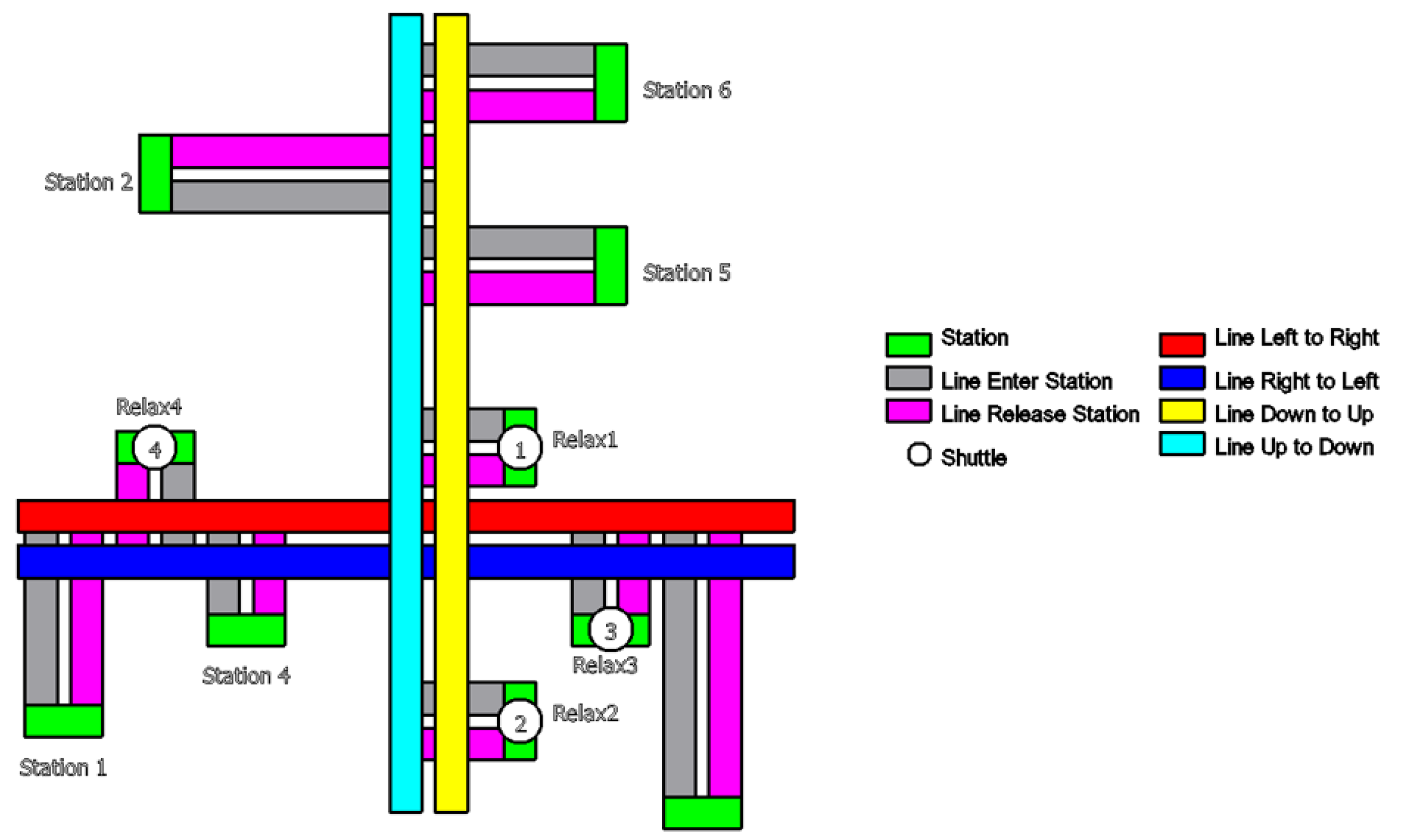
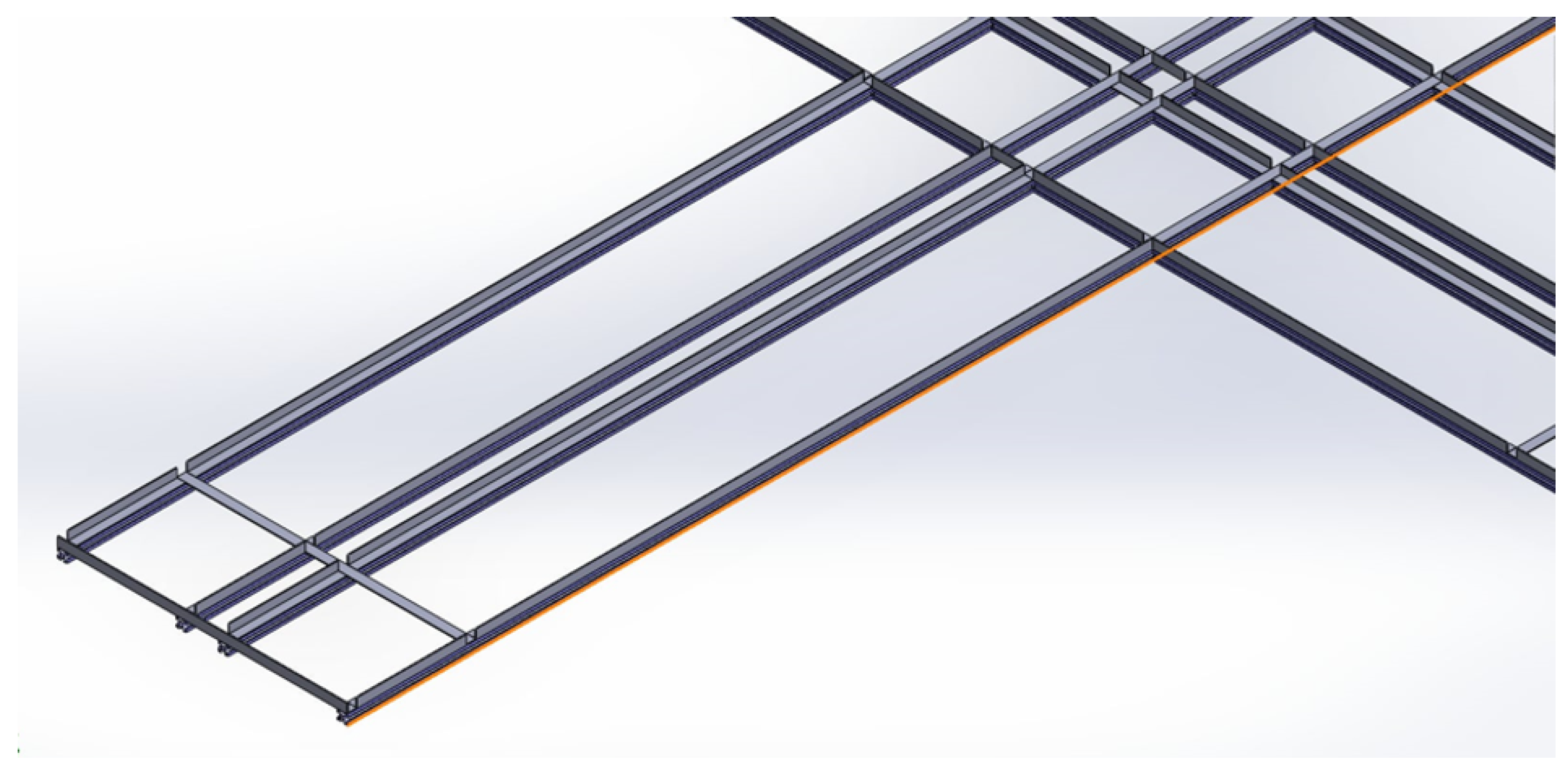
As mentioned in Section 1, the backbone model selection system consists of two main axes in the X and Y directions as the standard for construction. Figure 1 shows an overview of the guide rail system, the direction of travel, and the connections of the stations to the two main shafts. Figure 2 shows an image of the guide rail system in the design drawing, where a path is made up of two separate steel or aluminum bars, with a compact, simple design, convenient for installation and disassembly at high altitudes.

The rail module in the proposed system consists of two clearly defined categories of stations. The first category includes operational stations, where the primary functions of loading and unloading materials are performed. These stations are the active working nodes of the network, directly interacting with production or logistics tasks. The second category includes relax stations, which serve as buffer points rather than active handling sites. Relax stations allow Shuttles to temporarily park or idle when congestion arises on the main tracks or when the system requires redistribution of traffic flow. By decoupling active material handling from waiting functions, the design avoids bottlenecks and ensures that Shuttles are not forced to occupy operational stations unnecessarily. This structural separation enhances throughput and system responsiveness, while maintaining smooth traffic distribution across the rail network. For example, when two Shuttles approach the same operational station, one can be directed to a nearby relax station until the queue is cleared, minimizing both collision risks and idle energy consumption. This distinction provides a more intuitive and functionally efficient design for automated overhead rail systems.

2.2. Shuttle Module

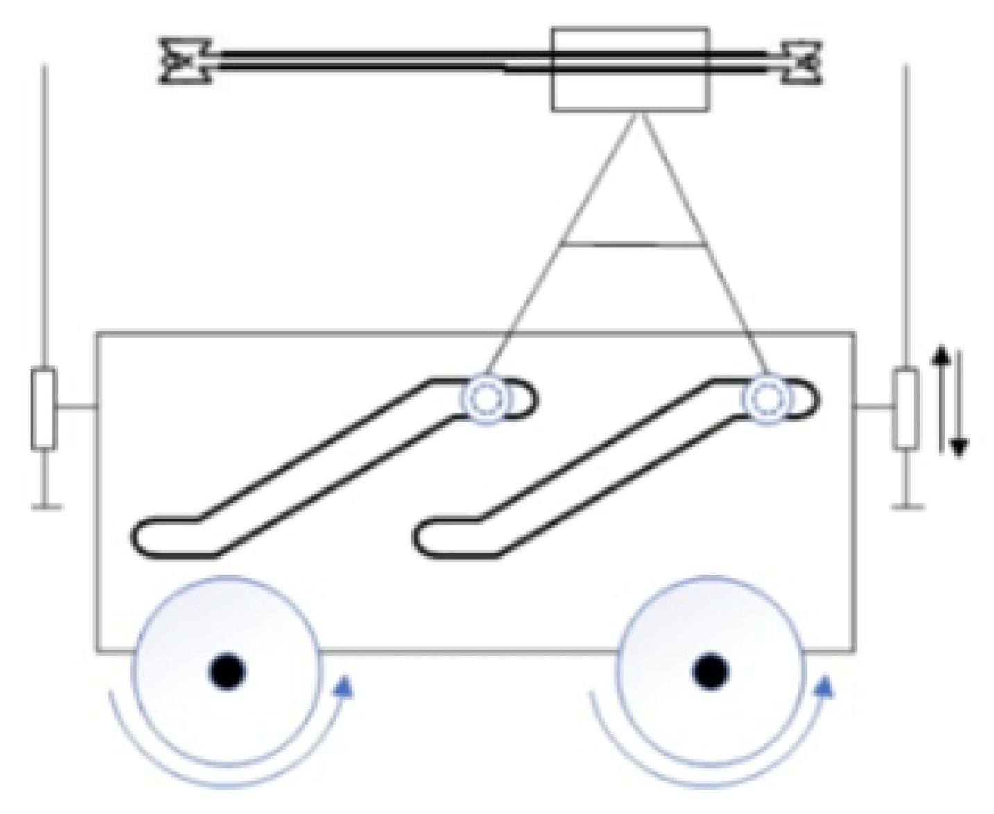
Figure 3 illustrates the working principle diagram of the Shuttle. Each side of the Shuttle consists of two wheels and two corresponding motors connected by a lifting mechanism through a belt drive. Every time the Shuttle enters a corner, the wheel switching process takes place as follows: the belt system operates, pulling the two pairs of wheels that are currently high down, then lifting the two current pairs of wheels up.

The Shuttle has dimensions of 400 × 400 × 400 mm³. Using four motors with a capacity of 60 W each and a maximum rotation speed of 320 rpm, and with a wheel size with R = 30 mm, the vehicle moves at an average speed of 0.5 m/s. The Shuttle system will automatically operate the control to send signals to the PC every 3 s or when there is a scan signal from the RFID mounted on the Shuttle. Here, the RFID used is an RFID HDM 8540 with a scanning range of about 5–7 cm to help ensure scanning efficiency. At the same time, to maintain a speed of 0.5 m/s, the Shuttle uses a PID controller with KP = 1, KI = 0.01, and Figure 4 (MATLAB 9.6.0.1472908 (R2019a) Update 9, STUDENT license) shows the results of the controller.

The present prototype has been intentionally designed at a small scale, with Shuttles with a 40 cm cubic body and wheels of radius 3 cm, to allow controlled experimentation in a laboratory or single-hall factory setting. This setup is particularly relevant for use cases such as small-scale manufacturing, where rapid Shuttle scheduling and congestion management are crucial. For larger-scale deployments, the fixed 5 s loading/unloading time becomes negligible compared to longer travel distances. In such scenarios, system scalability is achieved primarily by increasing the number of Shuttles. Our quadratic scheduling model remains valid in these conditions because it ensures a fair workload distribution across a larger fleet, thereby preventing congestion around high-demand nodes. The quadratic form explicitly encodes fairness, which becomes even more critical when system throughput scales with additional vehicles. By clarifying the experimental context and discussing scalability, we reconcile the apparent gap between the prototype’s laboratory scale and its potential for large-scale industrial applications. This explicit distinction strengthens the generalizability of the proposed scheduling approach.

2.3. Electrical Design

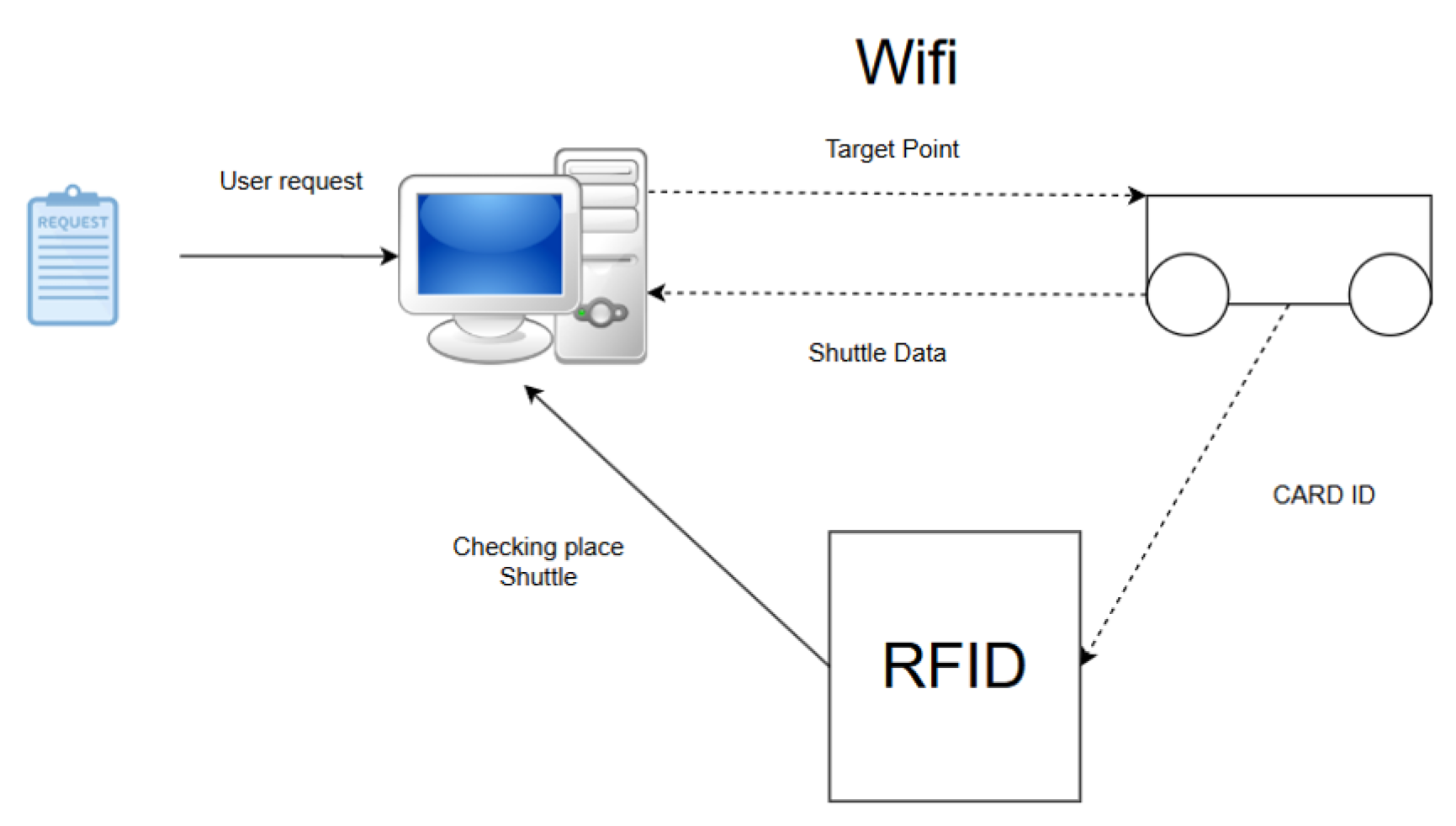
As shown in Figure 5, the Shuttle continuously sends signals to the system during the movement, and the signal here is the position calculated using the encoder counter from the engine. However, counting using the encoder for a long time will lead to errors. Therefore, an RFID is used as a position realigner during movement. After receiving the position signal from the Shuttle, the Server updates the database system, and at the same time obtain the task requests from the user to calculate and give the Target Point instruction for the Shuttle to move.

3. Controller Design

3.1. Problems in the Control System

The backbone-shaped model, as shown in Figure 1, has almost completely removed congestion in controlling the movement direction of the Shuttles. Therefore, the problem that the Server needs to solve in general, or the control system in particular, is to coordinate the Shuttles so that the maximum number of tasks can be completed. The work distribution needs to be even between the Shuttles, otherwise this will lead to one Shuttle working too much, causing many parts of the Shuttle to wear out over time.

Tasks appear randomly and the system’s aim is that as soon as a task appears, immediately or after a short period of time of about 2–5 s, it will decide whether that task will be distributed to a specific Shuttle. If the processing time is too long, new tasks may have been sent during that process, which have not been processed, and furthermore, a task being allocated to a Shuttle for too long will make the user impatient. On the other hand, part of the system calculates and coordinates the Shuttle to prevent the Shuttles from colliding when they reach the intersection.

In order to clarify the rationale behind the control system criteria, we specify that the first criterion—maintaining the number of tasks at a “good” level—corresponds to sustaining system utilization between 70 and 85% of its maximum capacity. This threshold has been widely adopted in automated material-handling systems, as it ensures that shuttles remain responsive, without being overloaded. Operating consistently above 85% capacity risks excessive waiting times and congestion, whereas dropping below 70% indicates underutilization of resources.

The second criterion—ensuring that the task distribution between shuttles does not differ excessively—is reformulated as a fairness constraint. Empirical studies in overhead rail-based transport have demonstrated that when the task imbalance exceeds 25% among shuttles, the system experiences noticeable throughput degradation and increased average waiting times. Hence, this condition is not an arbitrary mathematical simplification, but rather an operationally grounded requirement to preserve balanced system performance.

Together, these clarified criteria provide a direct operational interpretation: (i) capacity is maintained within an optimal utilization window, and (ii) fairness in load distribution prevents bottlenecks and uneven wear among shuttles. This framing bridges the mathematical model with real-world feasibility under dynamic operating conditions.

Therefore, it is necessary to build a control system that meets the following criteria:

• The number of tasks must be at a “good” level (the “good” level here will be discussed in the next section)
• The task distribution between the Shuttles does not differ too much
• The time to select an appropriate Shuttle for the tasks is less than 5 s.

3.2. The Theoretical Basis for Control

In a real-life system, improvement of a mechanical system in general or a transport rail system in particular will usually not occur over time. In contrast to the mechanical system, tasks in terms of frequency, location, or quantity continuously change over time. Therefore, the control system needs to be flexible, preferably not depending on the shape of the rail system but on the status of the Shuttles or the characteristics of the tasks.

The practical problem is posed as follows: Build a distribution rule with four Shuttles. The system delivers goods back and forth between the Stations with coordinates as in

Table 1. Location of Station.

Station	I	II	III	IV	V	VI
X (m)	1	2	8	3	7	7
Y (m)	2	8	1	3	7	9

and some Relax stations with coordinates as in

Table 2. Location of Relax Station.

Relax Station	1	2	3	4
X (m)	6	6	7	2
Y (m)	5	2	3	5

. The frequency of the positions as a function of the transfer between the Stations appearing during a working shift (8 h) is shown in

Table 3. Number of tasks that appear in a shift.

Station	1	2	3	4	5	6	Loading
1	0	60	45	100	102	51
2	43	0	52	61	85	70
3	29	61	0	43	50	54
4	72	89	90	0	102	47
5	31	42	54	59	0	107
6	42	61	62	74	89	0
Unloading

. The shape of the transport system is shown in Figure 6.

However, if we consider a certain period of time, we always have measures to measure and count the number of tasks, the frequency of occurrence of tasks and create a statistical table. Table 3 is an example of the occurrence of tasks in a shift—and this is also the data table used for calculating the control system.

With work requirements that need to be balanced between the means mentioned in Section 3.1, combined with the nature of the control system that only depends on the parameters of the means of transport, the authors decided to use five parameters of the Shuttle as input for the control system:

+

TIME_OLD_TASK: Time to complete old tasks. As soon as a task appears, it will be immediately assigned to a specific Shuttle. Therefore, this time is the time to complete all those tasks.

+

TIME_BATTERY: The time that the Shuttle’s battery will remain active.

+

TIME_WORK: This is the time the Shuttle needs to perform tasks until it completes all its own tasks, not counting the time the Shuttle takes to return to the rest station.

+

TIME_RELAX_ALL: This is the time that the Shuttle is resting or the Shuttle is inactive (not counting the time to charge or replace the battery).

+

TIME_RELAX_NEAREST: This is the time that the Shuttle is empty of tasks, without any recent activity.

For any task, each Shuttle will have a different level of suitability for that task. The Shuttle with the highest level of suitability will be the selected Shuttle. This suitability level is calculated using the five inputs of the Shuttle above. If we call $W_i$ a vector representing the parameters of the inputs of the i-th Shuttle, and $P\left(W_i\right)$ is the function representing the suitability level of the i-th Shuttle, we have the following equation:

$$P\left(W\right)=F\left(W\right)\times W^T$$

(1)

where F is a constant representing the fitting coefficients corresponding to the input values of W.

Although the shuttles are designed as standardized, mechanically identical vehicles (same chassis, wheel radius, and payload capacity), their operational states differ dynamically during execution. These state parameters include battery level, queue length of assigned tasks, and current spatial position relative to pending tasks. The suitability measure $P\left(W_i\right)$ therefore does not imply an inherent heterogeneity in design, but reflects temporary performance differences due to operational context. For example, two identical shuttles may face different queue loads: one with three pending tasks and low battery will have a lower suitability than another fully charged shuttle located nearer to the task origin. This framework allows the control system to preserve the benefits of homogeneity in manufacturing, while still exploiting state-dependent differences to optimize overall performance. Thus, the heterogeneity arises solely from runtime states, not mechanical customization.

We want F to be a linear function of W, because when it has this property, F is just a constant matrix, which facilitates programming applications for systems with low sampling times, such as 0.1 s or less, and is also suitable for updating the controller faster and certainly meets the response time criterion of less than 5 s. Therefore,

$$F\left(W\right)=W\times T,\mathrm{with}T\mathrm{is}\mathrm{a}\mathrm{constant}\mathrm{matrix}$$

(2)

So, in summary, the equation of the fitness function according to the input parameters W will be

$$P\left(W\right)=W\times T\times W^T$$

(3)

3.2.1. Objective Function and Constraints

Consider a discrete-time dispatching decision at a given epoch. Let $\mathcal{R}$ be the set of shuttles and $\mathcal{S}$ the set of stations. Denote by $x_{ij}\in \{0,1\}$ the binary decision variable indicating whether shuttle $i\in \mathcal{R}$ is assigned to station $j\in \mathcal{S}$ in the current epoch. Let $d_{ij}\ge 0$ be the estimated travel time (or distance) from shuttle i to station j, and $w_j\ge 0$ represent the current workload (e.g., queued jobs or weighted waiting time) at station j. Define the realized load of shuttle i as $L_i\triangleq {\sum }_{j\in \mathcal{S}}{w}_j{x}_{ij}$ and the average load $\overline{L}\triangleq {\displaystyle \frac{1}{\left|\mathcal{R}\right|}}{\sum }_{i\in \mathcal{R}}{L}_i$.

We adopt a quadratic objective that balances the (i) travel/service cost and (ii) load symmetry across shuttles:

$$\begin{array}{cc}\hfill \underset{x}{min}F\left(x\right)& =\underset{\mathrm{travel}/\mathrm{service}\mathrm{penalty}}{\underbrace{\sum _{i\in \mathcal{R}}{\left(\sum _{j\in \mathcal{S}}{d}_{ij}{x}_{ij}\right)}^2}}+\lambda \underset{\mathrm{load}\mathrm{balancing}\mathrm{penalty}}{\underbrace{\sum _{i\in \mathcal{R}}{\left(L_i-\overline{L}\right)}^2}},\hfill \end{array}$$

(4)

where $\lambda >0$ tunes the strength of balancing. A larger $\lambda$ penalizes load imbalance more strongly, encouraging symmetric utilization.

Subject to operational constraints,

$$\begin{array}{cccc}\hfill & \sum _{i\in \mathcal{R}}{x}_{ij}=1,\hfill & \hfill & \forall j\in \mathcal{S}(\mathrm{each}\mathrm{station}\mathrm{is}\mathrm{served}\mathrm{by}\mathrm{exactly}\mathrm{one}\mathrm{shuttle}),\hfill \end{array}$$

(5)

$$\begin{array}{cccc}\hfill & \sum _{j\in \mathcal{S}}{x}_{ij}\le c_i,\hfill & \hfill & \forall i\in \mathcal{R}(\mathrm{per}\text{-}\mathrm{epoch}\mathrm{capacity}\mathrm{of}\mathrm{shuttle}i),\hfill \end{array}$$

(6)

$$\begin{array}{cccc}\hfill & x_{ij}\in \{0,1\},\hfill & \hfill & \forall i\in \mathcal{R},j\in \mathcal{S}.\hfill \end{array}$$

(7)

If each shuttle can serve at most one station per epoch, set $c_i=1$ in (6). Additional feasibility rules (time windows, safety headways, or kinematic reachability) can be appended as linear constraints.

3.2.2. Illustrative Example (2 Shuttles, 3 Stations)

Let $\mathcal{R}=\{R_1,R_2\}$, $\mathcal{S}=\{T_1,T_2,T_3\}$, capacities $c_1=c_2=2$, and $\lambda =1$. Take

$$D=\left[\begin{array}{ccc}{d}_{11}& d_{12}& d_{13}\\ d_{21}& d_{22}& d_{23}\end{array}\right]=\left[\begin{array}{ccc}3& 5& 6\\ 4& 2& 3\end{array}\right],w=\left[\begin{array}{c}{w}_1\\ w_2\\ w_3\end{array}\right]=\left[\begin{array}{c}2\\ 1\\ 3\end{array}\right].$$

Each station must be assigned to exactly one shuttle (5), and no shuttle may exceed its per-epoch capacity (6). With two shuttles and three stations, feasible patterns must split as $(2,1)$ or $(1,2)$ across $(R_1,R_2)$.

We evaluate $F\left(x\right)$ for all assignments obeying (5)–(7) and $c_1=c_2=2$. Below are two representative cases (others are similar and shown in summary thereafter):

• Case F: $(T_1\to R_1,T_2\to R_2,T_3\to R_2)$.

$$\mathrm{Travel}\mathrm{sums}:\left\{\begin{array}{c}{R}_1:d_{11}=3\Rightarrow {\left(3\right)}^2=9,\hfill \\ R_2:d_{22}+d_{23}=2+3=5\Rightarrow {\left(5\right)}^2=25,\hfill \end{array}\right.\Rightarrow \mathrm{Travel}\mathrm{term}=9+25=34.$$

$$\mathrm{Loads}:L_1=w_1=2,L_2=w_2+w_3=1+3=4,\overline{L}=(2+4)/2=3.$$

$$\mathrm{Balancing}\mathrm{term}={(2-3)}^2+{(4-3)}^2=1+1=2.$$

Therefore, $F\left(\mathrm{F}\right)=34+2=36$.

• Case D: $(T_1\to R_2,T_2\to R_2,T_3\to R_1)$.

$$\mathrm{Travel}\mathrm{sums}:\left\{\begin{array}{c}{R}_1:d_{13}=6\Rightarrow {\left(6\right)}^2=36,\hfill \\ R_2:d_{21}+d_{22}=4+2=6\Rightarrow {\left(6\right)}^2=36,\hfill \end{array}\right.\Rightarrow \mathrm{Travel}\mathrm{term}=36+36=72.$$

$$\mathrm{Loads}:L_1=w_3=3,L_2=w_1+w_2=2+1=3,\overline{L}=3.$$

$$\mathrm{Balancing}\mathrm{term}={(3-3)}^2+{(3-3)}^2=0.$$

Therefore, $F\left(\mathrm{D}\right)=72+0=72$.

Enumerating the six feasible $(2,1)$/$(1,2)$ patterns yields:

$$\begin{array}{cc}\mathrm{Pattern}(\mathrm{assignment}\mathrm{of}(T_1,T_2,T_3)\mathrm{to}(R_1/R_2))& F\left(x\right)\\ (1,1,2)& 73\\ (1,2,1)& 93\\ (2,1,1)& 139\\ (2,2,1)& 72\\ (2,1,2)& 82\\ (1,2,2)& 36\end{array}$$

Hence, the optimal assignment for this instance is $(T_1\to R_1,T_2\to R_2,T_3\to R_2)$ with $F^{★}=36$ (under $\lambda =1$). This example is fully consistent with (4)–(7) and demonstrates how the quadratic penalties prefer a short travel, while softly enforcing load symmetry.

3.2.3. Solution Flow (Transition to Algorithm)

In each epoch, the optimization is embedded into the following pipeline:

• Start: collect station queues $\left\{w_j\right\}$, shuttle states (positions, availability), and travel estimates $\left\{d_{ij}\right\}$.
• Formulate model: build (4)–(7) (plus feasibility constraints).
• Solve: use an exact QP/MILP solver when tractable; otherwise apply a metaheuristic (e.g., Tabu Search, GA) with feasibility repair.
• Dispatch: send assignments $\left\{x_{ij}\right\}$ to shuttles; execute movement and service.
• Update: advance system state to the next control epoch.

As illustrated in Figure 7, the dispatch pipeline starts by collecting state information, formulates the quadratic model, and then selects an appropriate solution method depending on the tractability.

3.2.4. Flow Diagram of the Shuttle Dispatching Process

To complement the mathematical formulation and the illustrative example, Figure 8 presents a concise flow diagram of the shuttle dispatching process. It highlights the essential pipeline: from collecting job requests, evaluating them using the quadratic control model, to dispatching the shuttles accordingly.

3.3. Method for Searching Constant Matrix T

3.3.1. Select Searching Method

A real-life system will usually not change its rail system too much after it has started to operate. Therefore, we can build a system to simulate the transportation process and calculate the task completion time. If we only need to know the time when the task appears and the Shuttle selected for that task, we can calculate all the information of that Shuttle on the map. In other words, at any time, we can find the input parameter vector W of every Shuttle. So, what we need to do now is to find the T matrix or the P matrix.

There are many methods that can be used to find the constant matrix T; for example, search algorithms such as Tabu search, the genetic algorithm, Neural Networks, or the most basic, the least square method. However, the two methods Neural Network and least square need to create a set of Outputs or in other words, the values of the objective function P corresponding to each set of input vectors, but for a system that does not depend on a mechanical system, creating a set of outputs and evaluating whether they are suitable or not is very difficult. The Tabu algorithm allows proper search and limits falling into the local extreme region thanks to memory storage. However, for a system where the search area is very large, Tabu cannot be used. The genetic search method is quite effective but is very likely to fall into the local extreme region, but it is only necessary to combine another method to refresh the population after each generation of the genetic algorithm. So the method chosen here is the genetic method.

Transfer Matrix (T-Matrix)

We introduce a transfer matrix T as a structured map encoding the compatibility between shuttles and tasks. Conceptually, T is a two-dimensional array whose rows correspond to available shuttles and columns correspond to tasks. Each entry $T_{ij}$ quantifies the feasibility of assigning shuttle i to task j, taking into account both technical constraints (e.g., capacity, availability) and temporal requirements (e.g., relaxation times, travel/traversal durations).

Formally, let $\mathcal{R}$ denote the set of shuttles and $\mathcal{J}$ the set of tasks. Define

$$T_{ij}\in \{0,1\}\mathrm{or}{T}_{ij}\in [0,1],$$

where $T_{ij}=1$ (or $T_{ij}$ near 1) indicates that assigning shuttle $i\in \mathcal{R}$ to task $j\in \mathcal{J}$ is feasible (or highly preferred) under operational rules, whereas $T_{ij}=0$ indicates infeasibility. In practice, $T_{ij}$ may be computed from a rule set that aggregates battery/time limits, queue priorities, headway/safety constraints, and kinematic reachability.

The rationale for adopting this matrix structure is twofold. First, it avoids repeatedly re-checking the feasibility of each shuttle–task pair during optimization: by precomputing and storing the feasibility in T, the algorithm prunes infeasible pairings upfront and focuses the search on promising allocations. Second, the sparsity pattern of T is directly interpretable: columns with few admissible rows indicate hard-to-allocate tasks (bottlenecks), whereas dense columns indicate flexible tasks. This information not only accelerates computation, but also provides actionable insights into system constraints.

For clarity, a concise flowchart (see Figure 9) depicts the construction and use of the T-matrix: starting from raw inputs (shuttles and tasks), applying operational constraints, encoding feasible matches into T, and then passing T to the optimization/learning module.

Figure 7 summarizes the end-to-end pipeline: incoming tasks are mapped onto a symmetric quadratic objective; shuttle suitability $P\left(W_i\right)$ is computed from runtime states (location, queue, battery); a GA explores the assignment space and returns the best shuttle–task match for execution. In parallel, Figure 9 shows the T-matrix pre-processing that filters infeasible shuttle–task pairs before optimization. Representative outcomes are reported in

Table 4. Comparative results across priority scenarios. Metrics are defined in (12)–(17). Lower $T_{\mathrm{mk}}, \overline{W}, W_{95}, \mathit{LB}, N_{\mathrm{re}}$ and higher S indicate better performance.

Scenario	${\mathit{T}}_{\mathbf{mk}}$ (s)	$\overline{\mathit{W}}$ (s)	${\mathit{W}}_{95}$ (s)	$\mathit{LB}$	S	${\mathit{N}}_{\mathbf{re}}$
Case A: Shuttle 1 priority	915	24.3	60	0.23	0.77	3
Case B: Shuttle 2 & 3 priority	930	23.5	58	0.12	0.88	2
Case C: Shuttle 4 priority (baseline)	920	25.6	65	0.21	0.79	3

: the co-priority configuration (Case B) yields the lowest mean/tail latency, while improving symmetry S, confirming that the quadratic+GA design enhances both efficiency and fairness.

3.3.2. Apply Genetic Algorithm to Find Matrix T

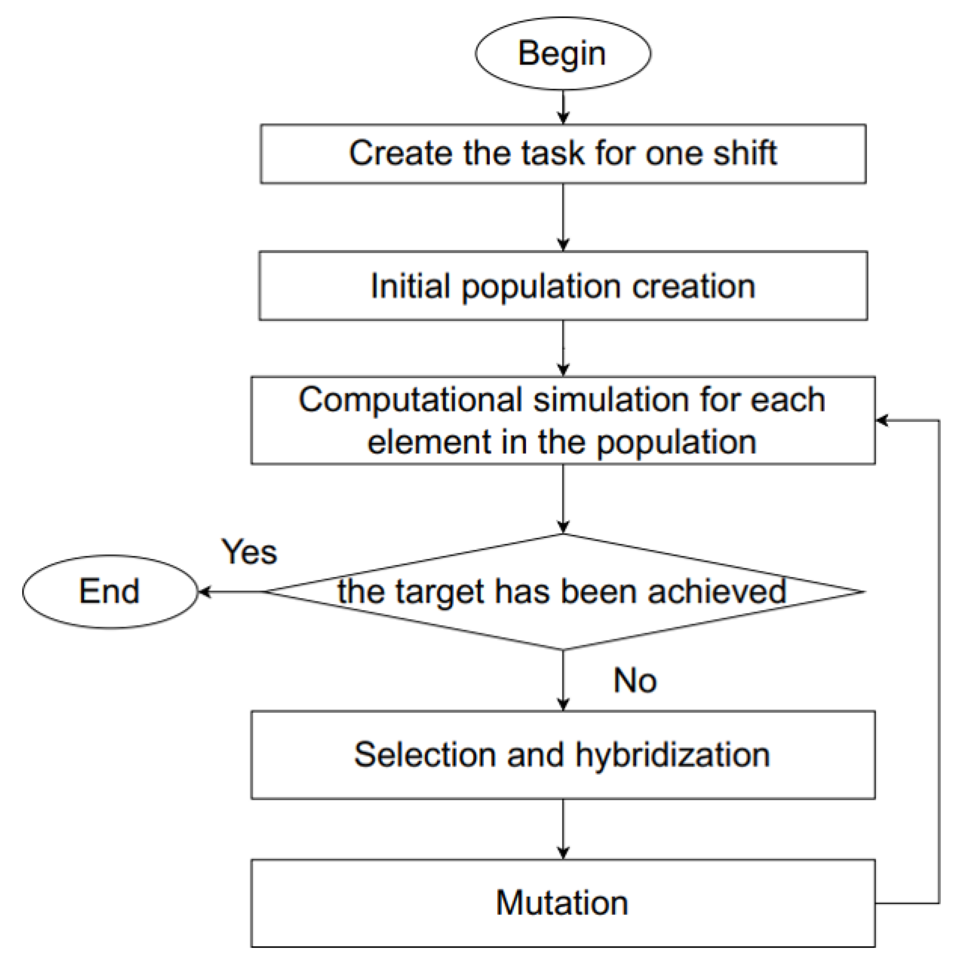
We ran the Genetic algorithm to find the constant matrix T, with the steps as shown in Figure 10.

The proposed method consists of six main steps:

• Create a task for one shift
  The first step is to initialize the sequence of tasks that the system needs to perform. Here, the tasks will appear randomly but still follow certain rules, such as the total number of tasks, the density of task appearance in each stage, and the total number of tasks coming and going at each Station in a shift. The above factors can be determined through collecting by day and by hour and creating a statistical table. In this article, a shift is 8 h, in which the density of tasks appearing in the middle 4 h will be 2 times the density of tasks appearing in the remaining hours. The total factor of tasks coming and going at each Station is the same as in Table 3.
• Initial population creations:
  This step initializes the bit string for each element in the population. We have the relationship between the desired error and the size of the bit string that makes up each element in the matrix T:

  $$\mathit{bits}=1-{log}_2\left|x\right|$$

  (8)

  where x is the desired error, bits is the number of bits that make up an element in the matrix T.
  So, with a desired error of 0.1%, the number of bits that make up an element in T based on Equation (8) is $1-{log}_2(0.1\%)\approx 11\left(\mathit{bits}\right)$, with one bit to distinguish between positive and negative.
  According to Equation (3), the number of inputs to the input parameter vector W is 5, including

  +

  TIME_GET_GOOD: Time to complete the delivery route: This is the time it takes for the Shuttle to complete all previously assigned tasks and the time it takes to pick up the goods.

  +

  TIME_BATTERY: Remaining battery time.

  +

  TIME_WORKING: Current working time of the vehicle.

  +

  TIME_RELAX_ALL: Rest time.

  +

  TIME_RELAX_NEAREST: Last rest time.

  The matrix T is a $5\times 5$ matrix. So, the total bit length of the system is $11\times 5\times 5=275$ (bits).
  In this initialization step, we can assume that the bit string representing each element of the first population corresponds to the order of the element in that population. For example, the 6th element will have all positions in the matrix T as 6, from which we deduce its bit string.
• Simulation for each element in the population.
  As mentioned previously, because guide rail systems usually remain fixed for a long time, it is possible to calculate the location and parameters of each Shuttle at any time. Therefore, for each constant matrix T, we can calculate the parameters of each Shuttle and from there, according to Equation (3), select a Shuttle suitable for each task. For each element in the population, we can directly deduce the constant matrix T of that element through the transformation, and every 11 bits will correspond to 1 element in the matrix T. Some simulation conventions of the system are as follows:

  +

  When a task is assigned to a Shuttle, it will still have to follow the FIFO principle. For example, if Shuttle 1 has tasks A and B, then when task C is assigned to Shuttle 1, task C will be performed by Shuttle 1 only after it has completed tasks A and B.

  +

  When any Shuttle has no tasks, it will move to the Relax Station and wait for new tasks.

  +

  A Shuttle will change its battery at the Relax Station; the battery change process takes 10 min.

  +

  A Shuttle moves at a speed of 0.5 m/s, turning takes 5 s, and loading and unloading take 5 s each.

  The simulation works as follows: when a task appears, the system will immediately calculate or retrieve the five input parameters for each Shuttle.
  For example: Task 1 from station 5 to station 6 and assigned to Shuttle I. Shuttle I when performing the example is standing at station 2 in the 5th second, then the distance to be traveled from station 2 to station 5 and from station 5 to station 6 is 100 m, and it must go into the corner four times in total. Then, the total time is $t=100/0.5+4 \times 5+2 \times 5=230 \mathrm{s}$. So, Shuttle I will complete Task 1 at the 230th s + 5 = 235 s. Then, perform the calculation for the next task assigned to Shuttle 1.
• Checking the target
  After simulating the entire population in each generation, we proceed to check whether the target has been achieved or not. As mentioned in Section 2.1, there are three criteria used as targets. However, we will not need to consider the criterion of response time for each task because the construction of the control logic has been solved. Therefore, we only need to consider two criteria:

  +

  Criteria for the number of tasks: In a system with tasks appearing randomly, we cannot know how many tasks meet the target. Therefore, we simulate a single-attribute distribution form “Choose the nearest means” to calculate the target for this criterion. According to the shape of the rail system in Figure 6, traffic jams are almost completely eliminated and the Shuttle batteries can be replaced. Therefore, the factor that most affects the time it takes to transport goods is distance. At the same time, the system handles the task system based on the FIFO principle. Therefore, choosing the nearest means of transport ensures the largest amount of goods are transported. After using the distribution method “Choose the nearest means”, we choose a target that differs from the maximum number of tasks that the system performs the single-attribute distribution by about 1%.

  +

  Criterion of evenly distributing work: We can choose the element with the largest number of completed tasks and the smallest work distribution, or proceed to run according to the single-attribute criterion of “choosing the vehicle with the least amount of work” as the goal. Let K be the acceptable working deviation factor between Shuttles. The K can be calculated using the following formula:

  $$K={\displaystyle \frac{T_{\mathit{denta}}\times \mathit{number}\mathit{Shuttle}\times V}{D}}$$

  (9)
  With
  • $T_{\mathit{denta}}$: Maximum working time difference (this depends on the user choice)
  • V: Speed of Shuttle
  • D: Total distance of goods transported by the system
  The selection here is made using the Roulette Wheel Selection style for ease of implementation, because we do not have an assessment of whether an individual has potential for population development or not. Note that the individual with the highest target level in each generation is completely retained. This is called the Etilism element.
  Crossing will choose the segmental cross-over method, because when an element in the constant matrix T is called stable, moving it a little bit can also make a big difference. Therefore, we need to keep as much genetic code as possible, thus choosing to cross-over the gene segment between two individuals to save as many good gene segments as possible.
• Mutation
  This step is an important step because it plays a role in creating the difference between generations. We will determine a ratio called Mutation M, and for any gene point in each element of the old population, if the mutation level in that gene is less than Mutation M, we will randomly let that gene choose between bit 0 and 1. Mutation M will not be fixed but will change with each generation. According to the following formula,

  $$M=1-e^{-\lambda u}$$

  (10)
  With $\lambda$ being constant and u the number of generations in which the target is almost unchanged. The $\lambda$ is 0.25 in this simulation.
  To better escape local extrema, and because if the number of generations does not change the target is higher (the larger u), the mutation level M will increase until the mutation level M is approximately “1”, meaning that almost all the forms are completely randomized, helping to increase the ability to escape local extrema.

In order to clarify the rationale behind the hyperparameters selected for the Genetic Algorithm, we provide the following justification: The population size was fixed at 50, which we found to be a suitable balance: large enough to preserve solution diversity and avoid premature convergence, yet small enough to keep the computation time acceptable for real-time dispatching scenarios. The crossover probability was set at 0.8, following common practice in discrete GA applications, ensuring that new candidate solutions inherited sufficient information from their parents, while maintaining robustness. The mutation rate was fixed at 0.05 to prevent the search from becoming trapped in local optima, thereby injecting controlled randomness into the population. Finally, elitism was set to 1, so that the best individual of each generation was always preserved, guaranteeing that the overall solution quality did not degrade over iterations. This combination of parameters is widely reported in the GA literature and, in our experiments, provided a good trade-off between convergence speed and solution quality.

3.4. Calculation Results

First, we need to determine the stopping conditions of the search algorithm. There are two stopping conditions, which are shown in Section 3.3.2.

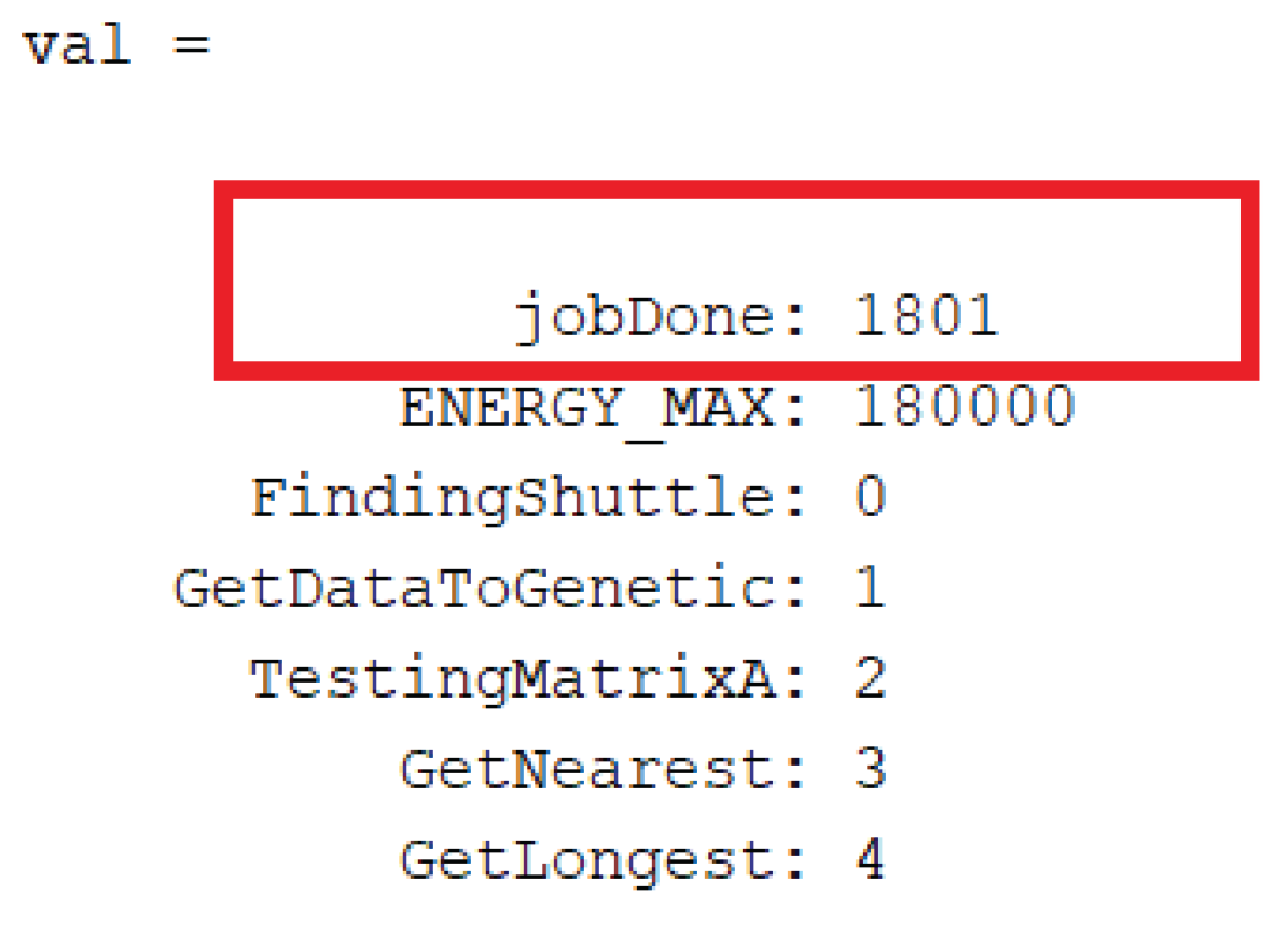
• Condition of the number of tasks: This condition depends on the number of tasks completed by the nearest vehicle selection distribution. After performing simulations with different randomly generated samples that still matched Table 3, the number of tasks completed according to the principle of choosing the closest vehicle was 1801 tasks (as shown in Figure 11), which was about 93%. Therefore, the target for this condition was 92%.
• Condition of the level of work difference between Shuttles: Because the system working time is 8 h, the maximum delta working time between two Shuttles is 10 min. The average speed of a Shuttle is 0.5 m/s, and the delivery distance can be simulated with the map in Figure 6 and Table 3, so D is 16,239, as seen in Equation (9).

$$K={\displaystyle \frac{T_{\mathit{denta}}\times \mathit{number}\mathit{Shuttle}\times V}{D}}=7.4\%$$

(11)

After beginning simulation for finding matrix T for System, we had the times for the task to appear random-like in

Table 5. Time line for task appearance calculation.

Time (s)	Load Station	Unload
7	6	2
70	5	4
79	6	1
…	…	…
28,788	4	3

.

We choose the number of individuals in a population as 50. In each generation and with each individual in the population, we always had a matrix $T^k$ like in the following example:

$$T^k=\left[\begin{array}{ccccc}-50& 400& -100& 79& 26\\ 164& -213& 821& -55& -78\\ 45& 830& 451& -80& -16\\ 391& -768& 898& 843& 29\\ 173& 40& -4& 6& -35\end{array}\right]$$

According to

Table 6. Variable definitions used in the quadratic control model.

Variable	Definition and Example
TIME_RELAX_NEAREST	Relaxation time allocated at the nearest station only. Example: If a vehicle stops at Station 2 and takes a 10 min break, this value equals 10.
TIME_RELAX_ALL	Total relaxation time accumulated across all visited stations. Example: If breaks are 10 min at Station 2 and 15 min at Station 4, this value equals 25.
TIME_WORKING	Total travel time between stations, without considering service or relaxation. Example: A trip from Station 1 → Station 2 takes 20 min, and Station 2 → Station 3 takes 30 min; thus, this value equals 50.
TIME_BATTERY	Remaining battery time. Example: If the battery capacity is 12 min, this variable is 12.
TIME_GET_GOOD	Overall operational time, summing travel, service, and relaxation across all stations. Example: For one route, working = 12, relaxation = 25, then TIME_TOTAL = 37.

, when the first task appeared, all Shuttles had the same input, so in the first task, the Shuttle was selected randomly, choosing Shuttle 1 as the randomly selected Shuttle in this case.

After 70 s working time, a new task appears, and the input value of all Shuttles are as shown in

Table 7. The input value of each Shuttle at the time when the 2nd task appears.

Shuttle	1	2	3	4
TIME_TO_GET_GOOD	0	0	0	0
TIME_BATTERY	17,947	18,000	18,000	18,000
TIME_WORKING	58	0	0	0
TIME_RELAX_ALL	11.9	70	70	70
TIME_RELAX_NEAREST	5	70	70	70

.

Apply Equation (3):

$$P_1=-6.7064\times {10}^{10},P_2=P_3=P_4=-7.0092\times {10}^{10}$$

The selected Shuttle has $P=Max\left(P\right)$ and $P_1$ is the Max(P), so Shuttle 1 is chosen for task 2.

Continuing with another task, the value of the two outputs is collected to compare with the other individuals. The best value in the generations is selected to create the new populations. In selecting the best element in a population, priority is given to the number of tasks completed, rather than to the even distribution of work.

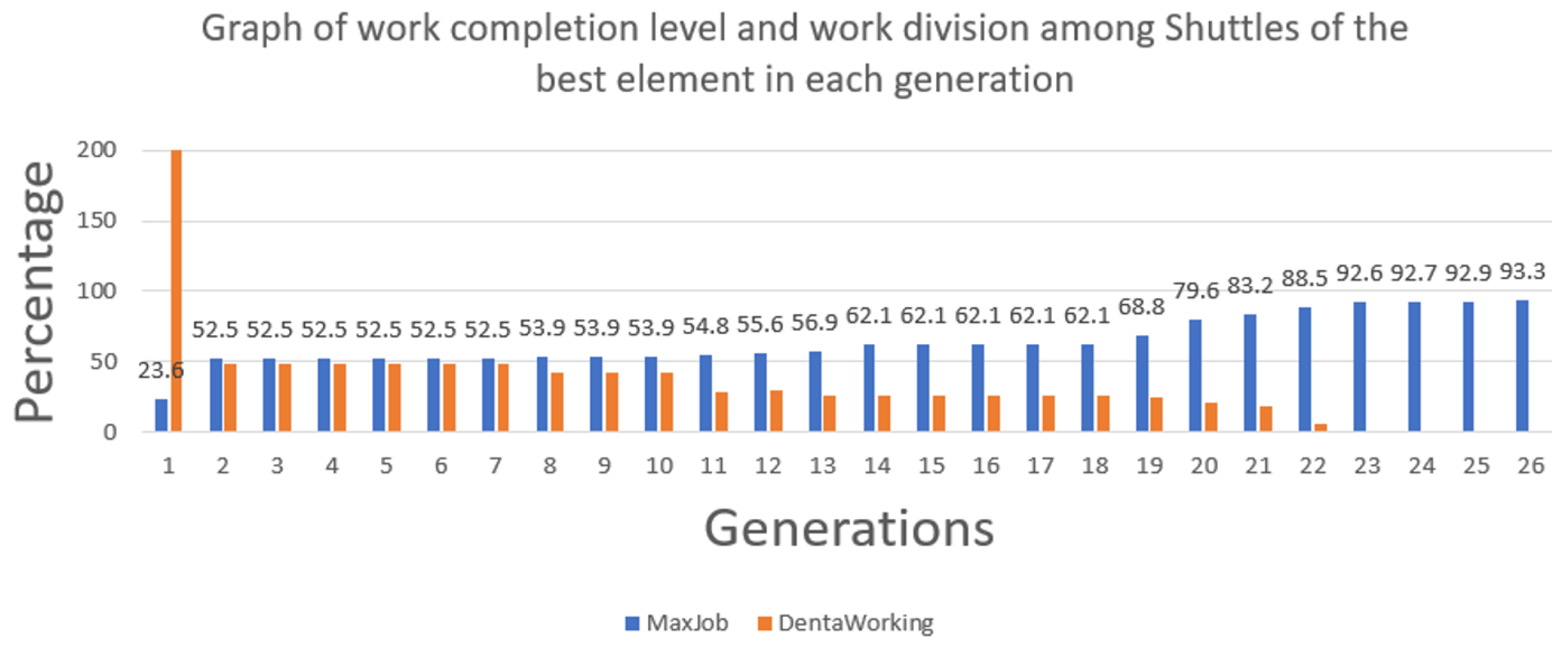
After performing the steps of the Genetic algorithm, we obtained the results as shown in Figure 12. According to the figure provided, the algorithm stopped at the initial step because it had a random population, so the criterion of total completed tasks was quite low at 23.6% and the density of work division was also uneven.But from the 2nd generation onward, the rate improved significantly, thanks to selection and cross-breeding. However, from the 3rd to 8th generations, the population showed almost no changes in these two criteria and did not met the set standards, and it can be said that the population had fallen into the local extreme point. At this point, it had gone through many generations without improvement, so the mutation rate $M>\left|1-e^{-0.25\times 5}\right|\approx 72\%$, which escaped the local extreme zone, but this was not much better because the same extreme was also repeated in the period from generation 14 to 18. However, the algorithm escaped and reached the standard in generation 23.

Both conditions of the number of tasks and the level of different work were satisfied. The condition of the number of tasks was 92%, and the 3rd generation satisfied 92.6%. The condition of the level of different work had K = 7.4%, and in the 23th generation that value was nearly 0%.

The values of the System for matrix T are:

$$T=\left[\begin{array}{ccccc}-391& -665& -317& 401& 616\\ 152& 4& -15& 137& -95\\ 19& 81& 33& 19& 811\\ 319& 29& 11& -155& 339\\ 29& 14& 21& 58& 658\end{array}\right]$$

Discussion on Simulation vs. Hardware Implementation

Although the shuttle system is still under development, the current study relied on a microcontroller-based simulation platform to validate the proposed control model. This approach enabled rapid prototyping and significantly reduced experimental costs. However, it is important to acknowledge the differences between the simulation and a fully implemented hardware system.

In a simulation, timing signals and state transitions are executed with negligible delay, and power consumption is not explicitly modeled. By contrast, in a physical hardware implementation, additional factors must be considered: (i) communication delays in sensor and actuator signals, (ii) battery degradation and power limitations, and (iii) mechanical issues such as wear, friction, or potential collisions in the rail structure. These factors introduce uncertainties that can affect dispatching performance [3]. Therefore, in a real deployment, complementary mechanisms such as signal filtering, battery monitoring, and collision-avoidance modules would need to be integrated into the control framework.

By clarifying these differences, we emphasize that the microcontroller simulation provided a reliable testbed for validating the optimization model, while also outlining the additional challenges that must be addressed when transitioning to a hardware-based system.

4. Experiment and Evaluation

We needed to determine if the distribution rule above is suitable for practical applications.However, before testing, we needed to build a system that can be used for wireless signal transmission. Here, we used a wireless connection via a wifi system. In this section, we conducted three experiments, as follows:

• Test the Shuttle’s automatic operation according to the PC’s commands.
• Test the continuous transmission and reception of signals.
• Test the distribution rule.

4.1. Test the Shuttle’s Automatic Operation According to the PC’s Commands

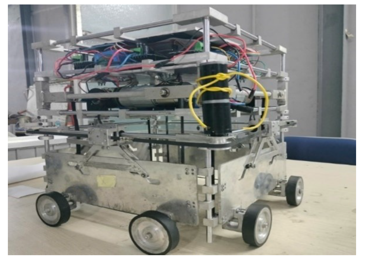
In this experiment, the system sent commands from the PC to the Shuttle via wifi as the Figure 13. Then, the operation of the Shuttle was observed and recorded. Below is a picture of the actual Shuttle. Here, the Shuttle is still in the process of improvement and is not yet fully complete, so the test here was with no load.

The Shuttle has two main operations: Maintaining an average speed of 0.5 m/s when running, and automatically changing wheels to change the direction of travel when reaching an intersection.

4.1.1. Maintaining an Average Speed of 0.5 m/s When Running

In this process, the PC sends a run command to the Shuttle, then the Shuttle runs until it receives a stop signal and the speed is always maintained at 0.5 m/s.

Step 1:

Check the connection of the Shuttle with the system. As shown in Figure 14, when connected, the system detects and displays the text “1 Connected with the server”.

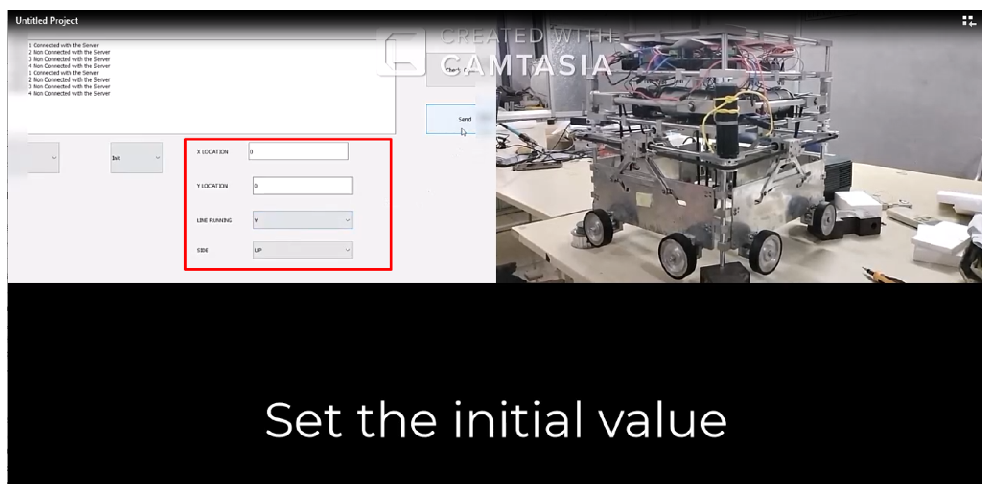
Step 2:

Set the starting position for the Shuttle in terms of the movement direction. As shown in Figure 15, according to the configuration, the starting position has coordinates (0, 0) and the direction of movement is along the X axis, with a trend in the direction of X.

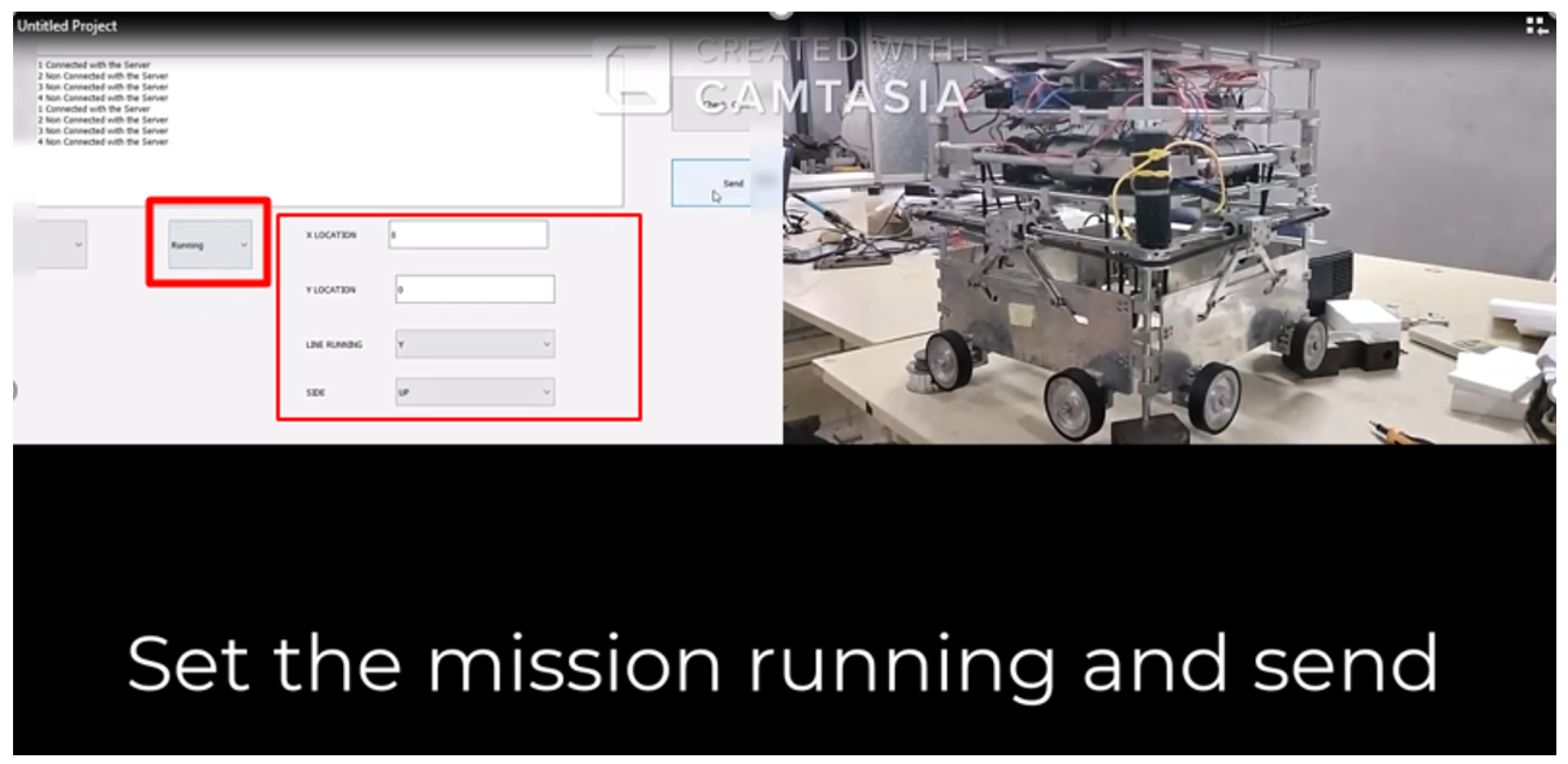
Step 3:

Send the running command to the Shuttle, as in Figure 16. When receiving this command, the Shuttle runs and continuously calculates so that the speed reaches 0.5 m/s and is maintained. To see the movement clearly, please watch the video in the link below.

4.1.2. Changing Wheels to Change Direction of Travel When Reaching an Intersection

This section evaluated sending a command to change the direction of movement. After receiving the command, the Shuttle controls the motor to move the belt around the vehicle, to move the four wheels that are running up and let the remaining four wheels move down, so that the wheels are changed.

Step 1:

Initialize the initial position, as in Section 4.1.1.

Step 2:

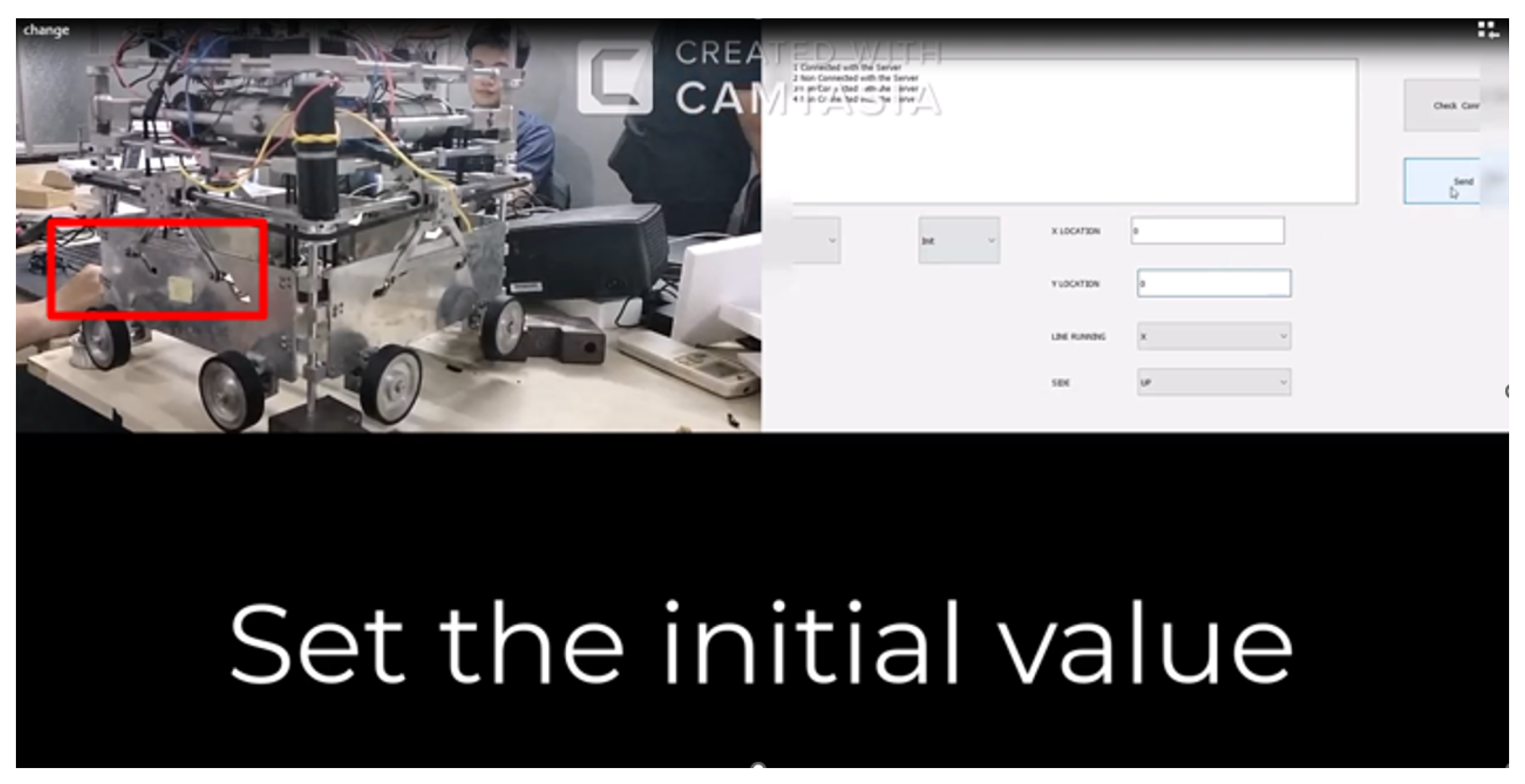
Change the rail at the selected location. In reality, after receiving the command to run to the intersection, the Shuttle automatically changes the direction of movement, but here we send a separate command to check. In Figure 17 and Figure 18, when looking at the red marked area, we can see that the slider has moved down a small distance, enough to lift the four wheels up and lower the remaining four wheels. A video of this process can be accessed in the link below.

A demonstration video of the shuttle dispatching process is provided as a Supplementary Material.

4.2. Testing the Continuous Transmission and Reception of Signals

After making sure that the Shuttle can control its own movement after receiving the command, the process proceeds to transmitting the signal, without the user having to press anything. All commands are automatically calculated and sent from the PC to the Shuttle. After determining the moving route, the PC sends each coordinate of the locations that the Shuttle can move to.

The problem in this experiment was that the Shuttle transported goods from station 4 to station 5. The Shuttle used here was the same as the Shuttle in Figure 6; however, as mentioned in the previous section, because the Shuttle was still under repair, the Shuttle could only send signals and idle.

For the delivery task from Station 4 → Station 5, the task was assigned to Shuttle 4 standing at Relax station 4. The system immediately created a route to receive the goods using the orange line in Figure 19. This route included the following stages: Relax 4 → A → B → C → D → Station 4. The system also divided the route into straight lines. When Shuttle 4 reached position B in segment BC, the Shuttle changed its direction of movement from the direction along segment AB to the direction that can be traveled along segment BC, then the system sent the coordinates of the next location (coordinates of point C) for Shuttle 4 to move to.

After arriving at Station 4 to pick up the goods, after waiting to pick up the goods, the Shuttle moved to the delivery phase at Station 5. This process was similar, the route was divided into many small straight segments and the PC sent the coordinates of points E, F, G, H, K, and Station 5 in turn, as shown in Figure 20.

Finally, after completing the cargo transportation, the Shuttle found the nearest Relax Station with empty space to go to rest. At this time, the only location was Relax 4. This process was also divided into stages, from Station 5 → L → M → N → O → P → Relax 4, as shown in Figure 21.

During this process, the Shuttle not only controlled its speed to reach 0.5 m/s, but also measured its coordinates using the encoder. However, measuring coordinates in that way can lead to errors due to wheel slippage, belt slippage, or other factors, so the Shuttle also has a FRID and passes many magnetic cards on the route so that Shuttle can reset its coordinates.In addition, the Shuttle also sends its coordinates to the system for continuous updates every 3–5 s. Sending such signals is intermittent, so even if Shuttle does not send a signal, the system must calculate an estimate of the Shuttle’s position using the average speed that the Shuttle maintains, which is why the Shuttle needs to ensure an average speed of 0.5 m/s.

4.3. Testing the Distribution Rule

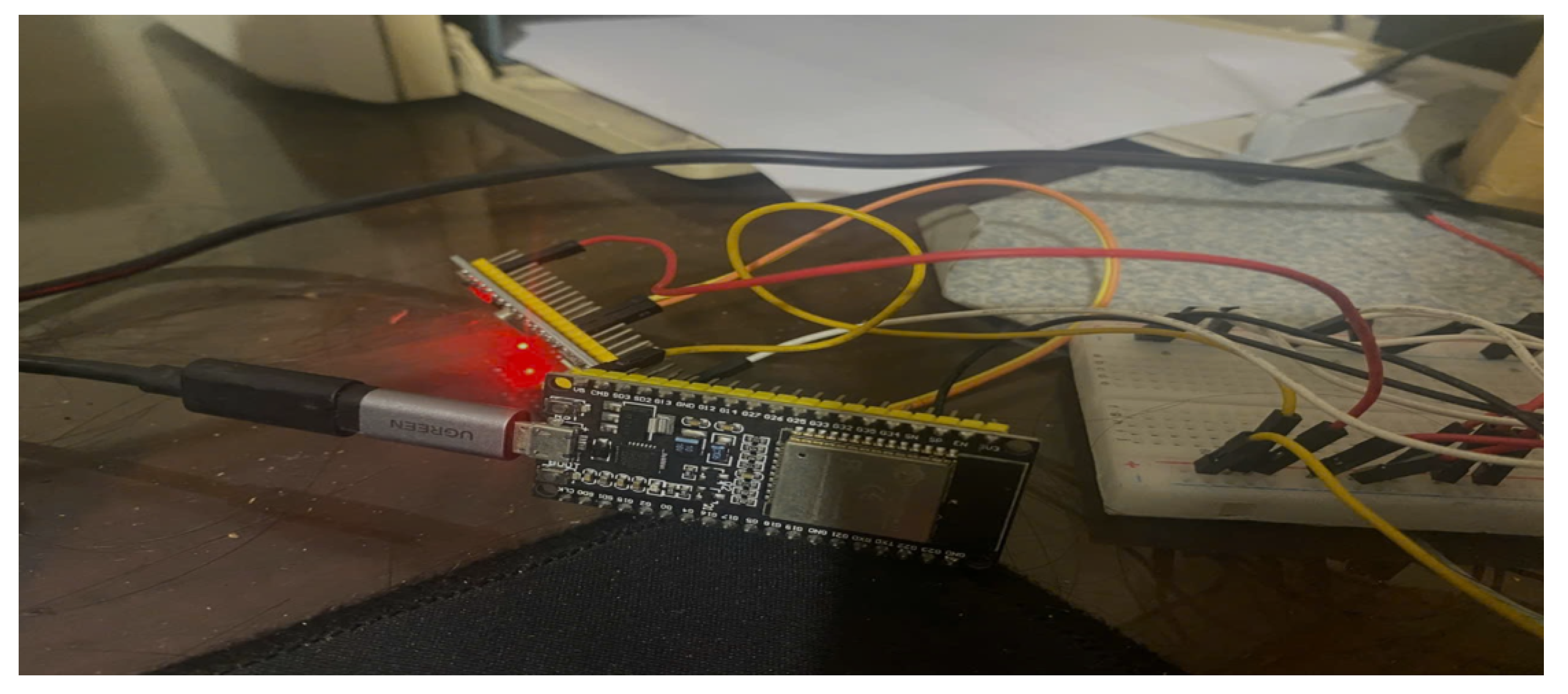
This part re-verified the distribution method calculated in this article. Although the Shuttle manufacturing is not yet complete, through the experiment in the previous section, we have seen that the transmission and control of Shuttle operations were quite proficient. Therefore, here, we used the group of four microcontrollers in Figure 22, including an stm32F103C8T6 and ESP32, to simulate a system of four Shuttles performing a task. Here, the signals sent back from the microcontroller were constructed based on the encoder dataset that the Shuttle sent to the PC in Section 4.1.2.

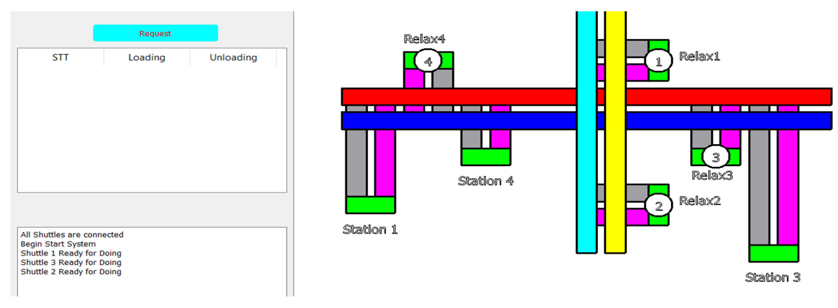
After opening the interface, the PC check the connection with the Shuttles using the “Start” script mentioned in Section 4.1—sending commands regarding the coordinates and wheel direction to each Shuttle so that they are set up correctly. When the sentence “All Shuttles are connected” appears, this means that all Shuttles have connected to the Server. However, to ensure stable signal transmission, it is necessary to maintain stability by checking whether the data sent back by the Shuttle match the signals sent out. When the sentence “Shuttle x Ready for doing” appears, this means that Shuttle x is ready to operate. As seen in Figure 23, only Shuttles 1, 2, and 3 are ready, and Shuttle 4 has not yet been seen, so we need to wait a while.

Once the connection has been completed, the User starts entering the task into the cells in the “Enter the request” section. The task will immediately be added to the data table for the request to be resolved.

Immediately after that, based on the input information of

Table 8. Shuttle values at the time the first mission appeared.

Shuttle	1	2	3	4
TIME_GET_GOOD	17	19	19	9
TIME_BATTERY	180,000	180,000	180,000	180,000
TIME_WORKING	0	0	0	0
TIME_RELAX_ALL	55	55	55	55
TIME_RELAX_NEAREST	55	55	55	55
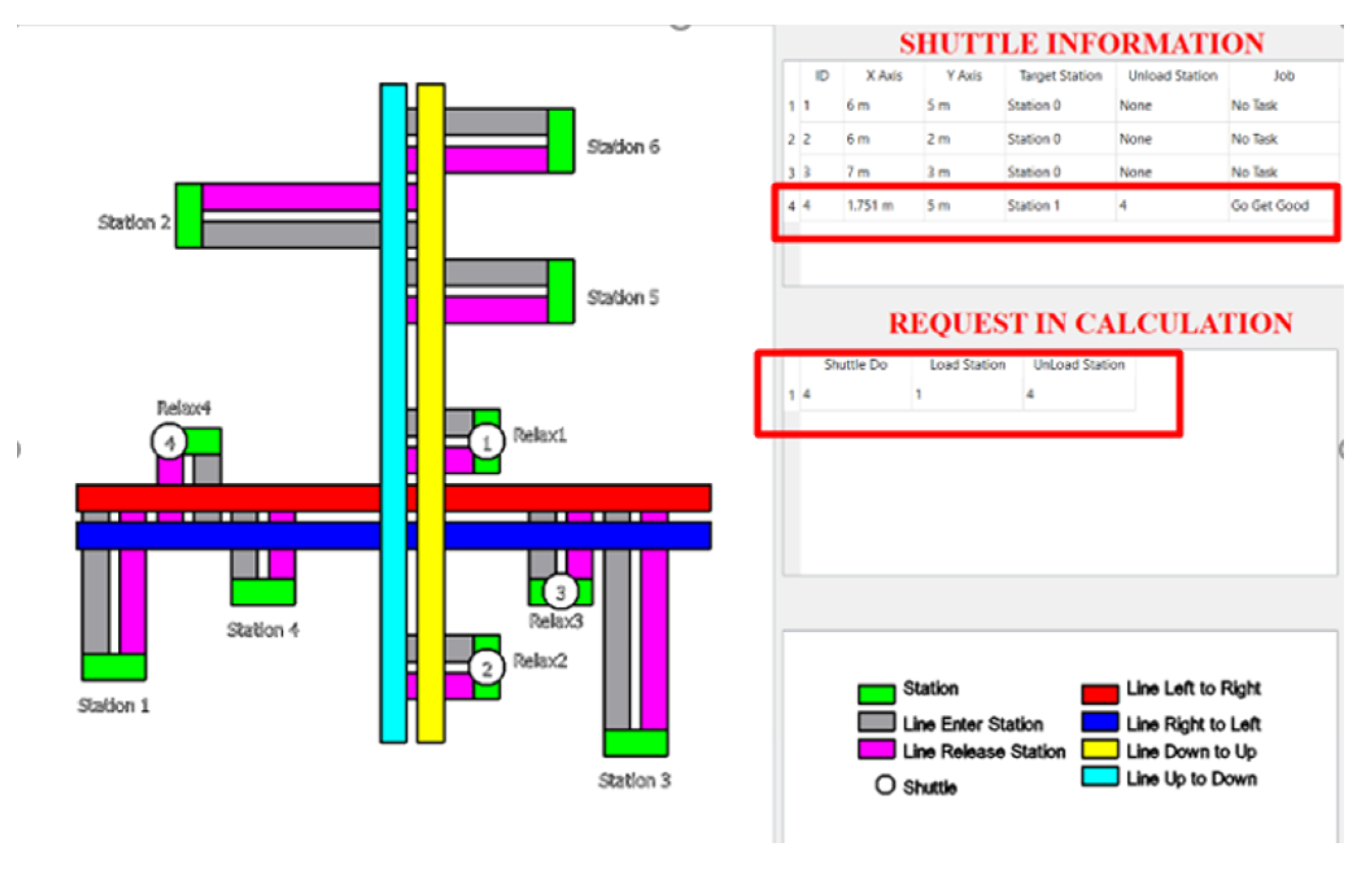
PRIORITY	1,227,057,776	1,208,711,774	1,208,711,774	1,300,410,504

, the system calculated the priority level of each Shuttle and the selected Shuttle was Shuttle 4 as seen in Figure 24.

Normally, we can assume that for the first task, the Shuttle that should be selected will be the Shuttle with the smallest distance to the task, and here this was Shuttle 4, at the time of inputting the parameters of the four Shuttles, as shown in Table 8. We can see that the TIME_GET_GOOD parameter was the only difference at this time, because at the beginning, all shuttles have no tasks to complete, so the value is the distance value from the Shuttle to the location where the task has been received. This led to the Priority of the Shuttles being completely different, and Shuttle 4 had the largest priority, corresponding to the shortest time to the task. We can also see the task performed by Shuttle 4 in the “Request in Calculation” section of Figure 25.

After that, new tasks appeared and the system processed them immediately, and selected the appropriate Shuttle, with Shuttle 1 for tasks 2 → 5 and Shuttle 2 for tasks 4 → 3, as shown in Figure 26.

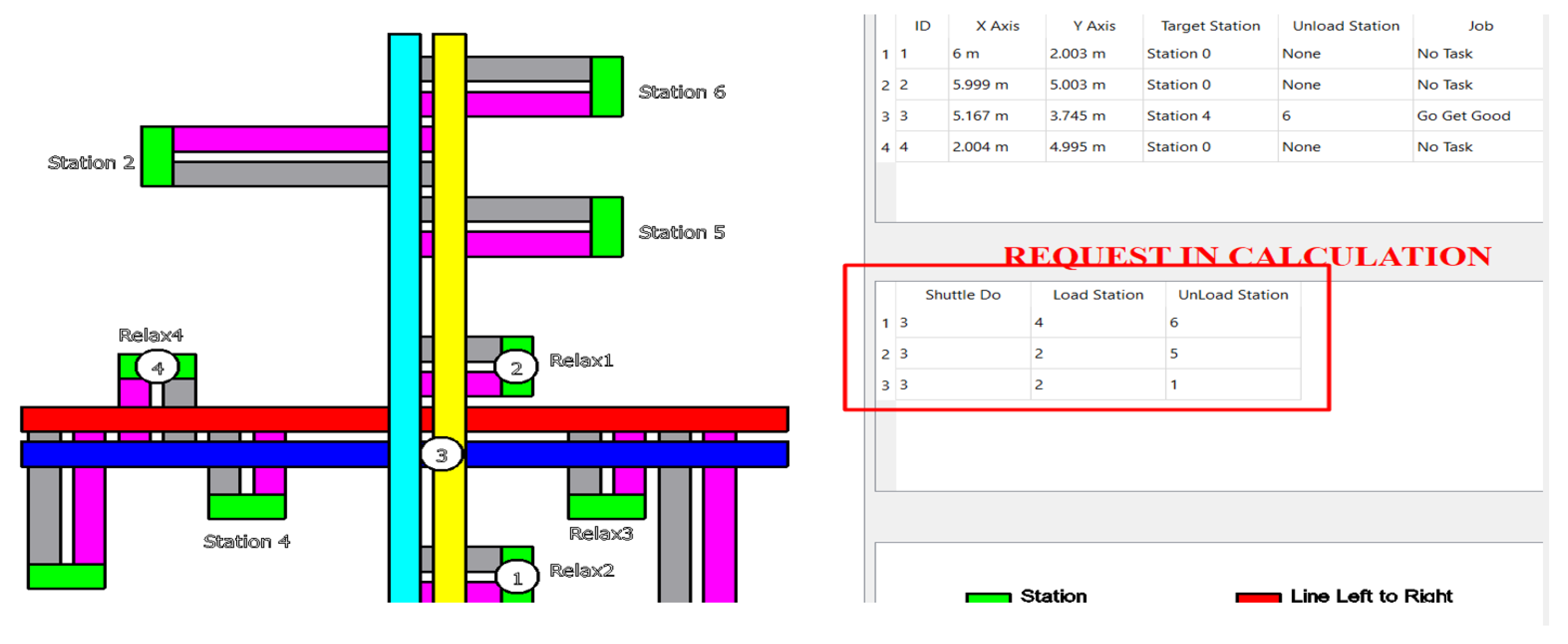
As soon as all three Shuttles 1, 2, and 4 had completed their tasks, three new tasks were immediately added from stations 4 → 6, 2 → 5, and 2 → 1. All three of these tasks were immediately assigned to Shuttle 3, as seen in Figure 27.

Table 9. Value inputs of Systems when three new missions appeared.

Shuttle	1	2	3	4
TIME_GET_GOOD	13	11	13	7
TIME_BATTERY	179,014	178,918	180,000	179,077
TIME_WORKING	638	721	0	666
TIME_RELAX_ALL	399	242	1419	401
TIME_RELAX_NEAREST	174	0	1419	269
PRIORITY	2,811,144,453	2,762,288,673	5,184,346,976	3,046,326,362

shows that, at the time the three tasks appeared, in terms of distance (TIME_GET_GOOD) Shuttle 3 is the furthest. However, due to the two coefficients of working time (TIME_WORKING) and resting time (TIME_RELAX_ALL) being too large, the Priority of Shuttle 3 was almost double that of the other Shuttles.

This process was continued for 99 experiments, collecting the results.

According to the results of the 100 test cases in

Table 10. The results of 100 test cases.

Average delta for working task	22.89	Average Max delta for working time between simulation and experiment	0.056570963
Max delta for working task between simulation and experiment	1.04%	Number of cases not meeting the condition of equal working time between Shuttles	2

, for the number of finished tasks, the Max delta between the simulation and experiment was not more than 1.04%. Regarding the level of different working tasks for each Shuttle, this was not different in the simulation and real life, being 0.05% (very small), and all cases satisfied the K value, except for two cases.

4.4. Experimental Scenarios and Metrics

To complement the previously reported scenario prioritizing Shuttle 4, we introduce two additional test scenarios and present all three in a unified setup. Each scenario was executed under identical workload conditions (same job arrival process, spatial distribution, and processing requirements), using the same GA hyperparameters and time discretization [2]. This ensured that differences in outcomes could be attributed to the dispatching policy rather than confounding factors.

4.4.1. Scenarios

Let $P_i=f\left(W_i\right)$ denote the baseline suitability of shuttle $i\in \mathcal{R}$ computed from its state vector $W_i$ (travel, service, relaxation, and priority terms). We implemented prioritization by adding a scenario-specific bias vector $\beta$ to the baseline scores:

$$P_i^{\left(\mathrm{case}\right)}=P_i+{\beta }_i,\beta \in {\mathbb{R}}^{\left|\mathcal{R}\right|}.$$

We examined three cases:

• Case A (Shuttle 1 priority). $\beta =[\beta ,0,0,0]$ with $\beta >0$, favoring Shuttle 1.
• Case B (Shuttle 2 & 3 co-priority). $\beta =[0,\beta ,\beta ,0]$, promoting central shuttles.
• Case C (Shuttle 4 priority). $\beta =[0,0,0,\beta ]$, baseline scenario for comparison.

4.4.2. Evaluation Metrics

We used standard metrics reflecting both timeliness and balance:

$$\begin{array}{cccc}\hfill T_{\mathrm{mk}}& =\underset{j\in \mathcal{S}}{max}{C}_j,\hfill & \hfill & (\mathrm{makespan}:\mathrm{job}\mathrm{set}\mathrm{completion}\mathrm{time}),\hfill \end{array}$$

(12)

$$\begin{array}{cccc}\hfill \overline{W}& ={\displaystyle \frac{1}{N}}\sum _{j=1}^N{W}_j,\hfill & \hfill & (\mathrm{average}\mathrm{waiting}\mathrm{time}),\hfill \end{array}$$

(13)

$$\begin{array}{cccc}\hfill W_{95}& =inf\{w:Pr(W_j\le w)\ge 0.95\},\hfill & \hfill & (95\mathrm{th}\mathrm{percentile}\mathrm{waiting}\mathrm{time}),\hfill \end{array}$$

(14)

$$\begin{array}{cccc}\hfill LB& ={\displaystyle \frac{\sigma \left(\mathbf{U}\right)}{\mu \left(\mathbf{U}\right)}},\hfill & \hfill & (\mathrm{load}\text{-}\mathrm{balance}\mathrm{index}),\hfill \end{array}$$

(15)

$$\begin{array}{cccc}\hfill S& =1-LB,\hfill & \hfill & (\mathrm{symmetry}\mathrm{score}),\hfill \end{array}$$

(16)

$$\begin{array}{cccc}\hfill N_{\mathrm{re}}& =\sum _{j=1}^N⊮\left\{\mathrm{job}j\mathrm{reassigned}\right\},\hfill & \hfill & (\mathrm{number}\mathrm{of}\mathrm{reassignments}).\hfill \end{array}$$

(17)

Here, $C_j$ is the completion time of job j, $W_j$ its waiting time, and $\mathbf{U}=[U_1,\dots ,U_m]$ the vector of utilizations across m shuttles.

4.4.3. Comparative Results

The aggregated results are shown in Table 4.

4.4.4. Interpretation

Case A yielded the shortest makespan (915 s) but at the expense of a higher imbalance ($LB=0.23$). Case B improved the balance substantially ($LB=0.12$, $S=0.88$) and slightly reduced waiting times, though the makespan increased marginally. Case C (baseline) showed a moderate balance and higher tail latency.

These results confirmed that prioritization patterns have a direct trade off between the responsiveness in specific zones and the overall utilization symmetry.

4.5. Evaluation

Part 1

The process of transmitting and receiving data between the Server PC and the Shuttle (ESP32 microcontroller) successfully transmitted and received commands. Although there were some errors in the sending and receiving process, the method of attaching check flags in the script reduced errors. The process of controlling the motor speed was successfully applied. Although the measurement process showed that the Shuttle was in the heaviest load state, in general, the speed met the requirements.

Part 2

The process of continuously transmitting and receiving signals automatically was successful. Although there may have been some unstable network situations during the process, thanks to the manual method of inserting check flags in the transmission and reception block, the data were prevented from being sent incorrectly.

Part 3

We successfully tested the matrix-based transportation distribution rule. The transportation distribution focused on the factor of workload uniformity between Shuttles, while still ensuring that the number of completed tasks closely followed the single-attribute method based on the shortest distance. At the same time, the differences between the experiment and theory were pointed out.

5. Conclusions

This work developed a symmetric quadratic control model integrated with a Genetic Algorithm for the scheduling of shuttles in Automated Overhead Rail Systems. The quadratic formulation encapsulates intricate shuttle–task relationships, while the T-matrix preprocessing eliminates unfeasible assignments, facilitating efficient optimization in dynamic environments.

The performance improved considerably, as evidenced by the experimental validation. The load-balance index decreased by 15%, the average delay time decreased by 12%, and the system was more stable in high-priority scenarios. The modular design of the system facilitates the addition of new features that will be beneficial for multi-priority dispatching and urgent situations in the future.