Mixer Temperature Prediction via Decomposed Transformer and xLSTM with Physical Constraints

Abstract

During high-altitude simulation tests, the accurate reproduction of environmental conditions directly affects the ability to reliably evaluate the engine’s performance under simulated high-altitude conditions. Traditional physical models, though interpretable, often fall short in handling nonlinear dynamics and time-delayed effects caused by disturbances such as abrupt flow rate fluctuations. For this problem, this work proposes a novel hybrid modeling framework that integrates physical principles with deep learning architectures. The proposed approach incorporates three key innovations. First, a physics-guided residual learning scheme is introduced, where the theoretical outlet temperature derived from energy conservation laws and assumptions of symmetric inlet mixing serves as a prior, and a data-driven model corrects residual deviations. Second, a multiscale feature extraction module is constructed by combining a Transformer with DWT, capturing both long-term regularities and short-term fluctuations that often exhibit quasi-symmetric patterns in structured systems. Third, a perturbation-aware memory structure is designed, fusing a Transformer branch for long-term dependency modeling with an extended LSTM (xLSTM) branch for short-term dynamic sensitivity. The experimental results on real-world test datasets demonstrate that the proposed hybrid model significantly outperforms traditional physical models. Specifically, it achieves an MAPE of 0.0156 and a R² of 0.9867, indicating high predictive accuracy. The model not only achieves superior prediction accuracy but also preserves physical interpretability, making it a promising solution for intelligent control in industrial mixing systems.

1. Introduction

Gas mixers are widely used in various industrial applications, serving as a critical component in systems where precise blending of different gas streams is required. From chemical reactors [1] and HVAC systems [2] to medical ventilators and fuel reformers, gas mixers ensure that downstream processes receive gases with desired thermodynamic properties. In the aerospace industry, the flight environment simulation intake system is the core subsystem of the altitude ground test facility, which is used to simulate the intake environmental conditions of aero-engines operating at cruising altitudes [3,4]. Within the flight environment simulation intake system, the mixer is responsible for blending high-pressure cold air, hot air, and ambient air to create the desired temperature and pressure conditions for aero-engine inlet testing. The thermal condition at the mixer outlet not only determines the accuracy of simulated flight conditions but also influences key parameters such as engine thrust, fuel–air ratio, and thermal loads on engine components [5]. As such, ensuring accurate prediction and control of the mixer outlet temperature is of paramount importance for reliable engine testing and evaluation.

However, achieving precise thermal simulation in such mixers remains a technical challenge. The nonideal behavior of the airflow, energy losses, uneven mixing, and slow mixing under complex real-world conditions cause substantial discrepancies between the actual outlet temperature and the theoretical temperature [6,7]. From an analysis of existing high-altitude engine test data, the mixing rate in the mixer for different operating points ranges from 0.3 to 0.85 °C/min. Traditional modeling approaches—often based on steady-state energy conservation and enthalpy difference methods—assume ideal mixing and ignore spatial non-uniformity, temporal delay, and thermal inertia introduced by the mixer’s internal geometry and unsteady operating conditions. These simplifications are inadequate for reflecting transient dynamics caused by rapid changes in valve adjustments or flow disturbances commonly encountered during test campaigns. Moreover, the thermal behavior of the system is further complicated by several factors, including large-volume flow within the mixer cavity, flow separation before it enters the mixer, and imperfect interactions between the mixing jets. These phenomena introduce nonlinearities and spatial–temporal variations that make predictions based solely on first-principles models prone to significant errors and instability.

Recent studies have demonstrated the effectiveness of hybrid modeling and Physics-Informed Machine Learning (PIML) in environmental and industrial time-series prediction. For example, Bagheri et al. [8] developed a hybrid framework for modeling soil water content that integrated deep learning models (e.g., LSTM, random forest) with a simplified hydrological model through residual learning and physics-informed neural networks, achieving improved accuracy while preserving physical interpretability. In another study, Naeini and Snaiki [9] proposed a physics-informed approach for simulating time-series wave runup by combining the computational efficiency of the Surfbeat (XBSB) mode with the accuracy of the non-hydrostatic (XBNH) mode of the XBeach model, using a conditional generative adversarial network to incorporate physics-based knowledge into the learning process.

In order to improve the prediction accuracy of mixer outlet temperature, this work proposes a novel hybrid modeling framework integrating domain physical knowledge with time-series learning techniques. The major contributions of this work are summarized as follows:

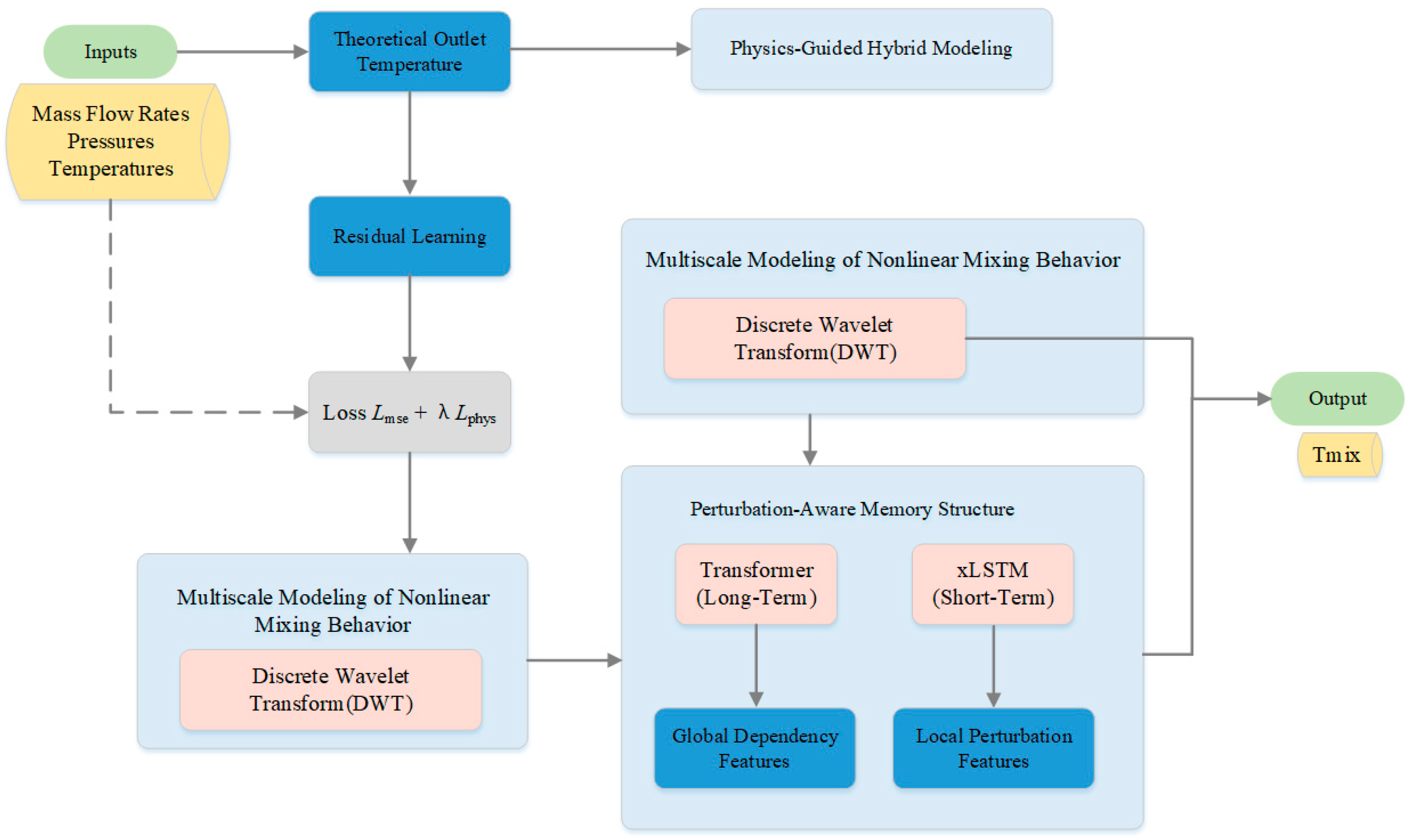
• The theoretical outlet temperature, calculated based on energy conservation, is embedded physically prior to the modeling process. Instead of directly predicting temperature, the model focuses on learning the residual error between measured and theoretical values. This residual learning framework improves generalization capability, enhances model stability under complex working conditions, and ensures the predictions remain physically interpretable.
• To accurately model both the long-term delayed effects and the short-term disturbances in the outlet temperature sequence, a dual-path structure is designed. The differential Transformer captures flow-induced abrupt changes by processing first-order differences of input sequences, effectively enhancing sensitivity to perturbations. The xLSTM branch simultaneously captures local nonlinear dynamics and slow-varying trends, achieving fine-grained multi-scale temporal representation.

The remainder of this paper is organized as follows: Section 2 reviews existing research on thermal modeling of mixers and temperature prediction methods. Section 3 models the prediction problem and analyzes the available data. Section 4 presents the architecture and principles of the proposed hybrid prediction model. Section 5 discusses experimental results based on measured data. Finally, Section 6 concludes the work and outlines future research directions.

2. Related Works

2.1. Mixer Modeling of Engine Test Systems

Extensive studies have been conducted on the temperature regulation process of high-altitude simulation systems. Zhu et al. [10] simplified the mixer as a volume model without considering airflow mixing and heat transfer, while Zhu et al. [4] further proposed a multi-volume model incorporating these factors for improved accuracy. Wang et al. [11] optimized mixer structures to address non-uniform airflow distribution at the outlet. Zhu et al. [12] analyzed dynamic heat transfer during high-altitude heating tests, considering local heat loss. Montgomery et al. [13,14] explored how metal mass, cavity volume, and airflow states influence intake temperature change in turbine engine test cells. To address the problem of substantial temperature delays in the flight environment simulation system for altitude ground test facilities, Zhu [15] investigated the effects of flow ratios and structural parameters on cold and hot airflow mixing characteristics. Most existing studies still focus on the influence of heat transfer processes, while lacking in-depth consideration of the coupling relationships among internal system variables.

2.2. Temperature Prediction Method

In the modeling process, various disturbance factors cannot be corrected within the original mechanistic model. However, hybrid modeling methods based on mechanisms and data-driven methods effectively solve this problem [16,17]. Ning et al. [18] demonstrated improved spacecraft control system modeling using mechanism-data fusion. Peng [19] addressed nonlinear and strong hysteresis issues in the heating process of vacuum sintering furnaces by combining both mechanistic analysis and data-driven methods. Yu [20] developed an outlet temperature prediction model for a decomposition furnace using elastic networks and LSTM, achieving precise control. Adam Kula et al. [21] compared machine learning methods for data center temperature forecasting in the warm corridor of the data centre. Zhang et al. [22] integrated mechanism models and stacking frameworks for accurate parameter prediction of a condenser system. Yan et al. [23] proposed a hybrid ALSTM model for predicting solar collector outlet temperatures. However, the current methods still fall short of fully meeting the requirements for high-accuracy and robust outlet temperature prediction under complex operating conditions.

3. Problem Modeling and Data Analysis

The mixing of two air streams with different temperatures, pressures, and flow rates is a highly coupled and dynamically evolving thermodynamic process. To more effectively characterize the input–output behavior and dynamic features of this process, this chapter approaches the problem from a system modeling perspective. Based on original data, this section conducts a comprehensive analysis of the temporal variation characteristics of the mixer outlet temperature. Furthermore, it critically evaluates the strengths and limitations of different modeling paradigms, thereby laying a theoretical foundation for the selection and design of predictive models in subsequent stages.

3.1. System Description and Data Acquisition

This study focuses on the intake temperature regulation subsystem within the altitude ground test facility. The original data used in this study are derived from high-altitude test data of a certain aero-engine, with a sampling period of 0.2 s. A total of 19 characteristic variables were recorded, covering the pressure, temperature, and mass flow rate of two intake streams (ambient air and cooled air), secondary flow, and the mixer outlet. The variables are listed in

Table 1. Measurement parameters.

Flow/Location	Mass Flow Rate	Pressure	Temperature
Ambient Air	$W_n$	$P_{n1}$$, P_{n2}$$, P_{n3}$	$T_{n1}$$, T_{n2}$$, T_{n3}$
Cooled Air	$W_c$	$P_{c1}$$, P_{c2}$$, P_{c3}$	$T_{c1}$$, T_{c2}$$, T_{c3}$
Mixer Outlet	-	$P_{mix}$	$T_{mix}$
Secondary Flow	$W_{sec}$	$P_{sec}$	$T_{sec}$

. Due to proprietary constraints, the original dataset cannot be publicly released. To facilitate reproducibility, we provide statistical characteristics of the data: input parameters (e.g., $W_c$, $W_n$, $P_{n1}$) exhibit rapid temporal variations, while the target output parameter ($T_{mix}$) shows a delayed response and slow-varying behavior.

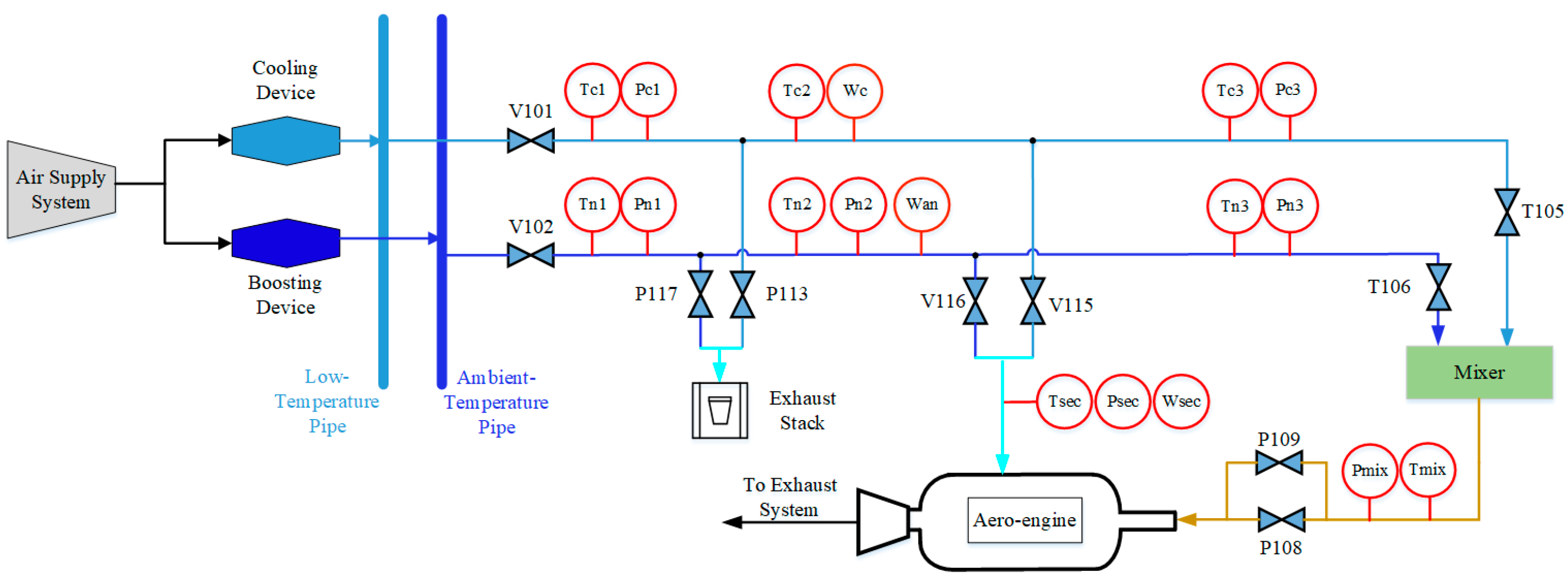
The system schematic diagram is shown in Figure 1, with all measurement points clearly labeled. The air supply system delivers two streams of air with distinct temperatures and pressures, which are mixed within the mixer. Flow rate and pressures of each stream are precisely regulated via control valves to ensure that the mixed airflow meets the target temperature and pressure requirements before being supplied to the chamber for aero-engine tests. The aero-engine under test is a twin-spool turbofan engine with a maximum rotational speed of 37,000 rpm. The secondary flow is used for component cooling and does not exceed 5% of the mainstream flow. Structurally, the mixing unit exhibits geometrical and functional symmetry, with two symmetric inlets and one outlet—facilitating balanced energy and mass exchange under ideal conditions.

Assuming the confluence of two airstreams with different temperatures, pressures, and flow rates within the mixer. Under the assumption of a steady-state mixing process, the mass conservation principle can be expressed as follows [24]:

$$m_1+m_2=m_{mix}$$

(1)

The energy conservation equation can be expressed as:

$$m_1{C}_{p1}{T}_1+m_2{C}_{p2}{T}_2=m_3{C}_{p\mathrm{m}ix}{T}_{\mathrm{c}al}$$

(2)

Combining Equations (1) and (2), the mixed temperature is obtained:

$$T_{cal}={\displaystyle \frac{m_1{C}_{p1}{T}_1+m_2{C}_{p2}{T}_2}{\left(m_1+m_2\right)·C_{pmix}}}$$

(3)

where $m_1$, $m_2$, and $m_3$ represent the mass flow rates of the first, second, and mixed airflows, respectively, in $\mathrm{k}\mathrm{g}/\mathrm{s}$, $C_{p1}$, $C_{p2}$, and $C_{p3}$ are the specific heat capacities of the first, second, and mixed airflows, respectively, in $\mathrm{J}/\left(\mathrm{k}\mathrm{g}·\mathrm{K}\right)$, and $T_1$, $T_2$, and $T_3$ are their corresponding temperatures in $\mathrm{K}$.

Assuming that the specific heat capacity of air remains constant during the mixing process, Equation (3) can be simplified as:

$$T_{cal}={\displaystyle \frac{m_1{T}_1+m_2{T}_2}{\left(m_1+m_2\right)}}$$

(4)

To eliminate the influence of the secondary flow, the mass flow rate of the ambient air and the cooled air within the secondary flow are calculated using Equations (1) and (4):

$$W_{nsec}={\displaystyle \frac{\left(T_{sec}-T_{c2}\right)·W_{sec}}{T_{n2}-T_{c2}}}$$

(5)

$$W_{csec}=W_{sec}-W_{nsec}$$

(6)

where $W_{nsec}$ represents the mass flow rate of ambient air in the secondary flow, and $W_{csec}$ represents the mass flow rate of cooled air in the secondary flow. The meanings of other symbols are as shown in Figure 1. The effective mass flow rates of the two incoming air streams at the mixer are determined by subtracting the corresponding secondary flow contributions.

While Equations (1)–(4) theoretically define the ideal outlet temperature based on symmetric energy exchange between two streams, practical systems deviate from symmetry due to factors such as thermal inertia, volumetric lag, and imperfect mixing. Therefore, a deviation term $ϵ$ is introduced:

$$T_{cal}={\displaystyle \frac{m_1{T}_1+m_2{T}_2}{\left(m_1+m_2\right)}}+ϵ$$

(7)

3.2. Statistical Characteristics Analysis of Mixer Outlet Temperature

To analyze the dynamic behavior of the mixing temperature, this section performs the following statistical analyses on $T_{\mathrm{m}ix}$:

3.2.1. Stationarity Analysis

The Augmented Dickey–Fuller (ADF) [25] test is employed to evaluate the stationarity of the outlet temperature sequence $T_{\mathrm{m}ix}$. This test determines whether a time series contains unit roots, which are indicative of non-stationarity. In contrast, a stationary series does not contain unit roots. The ADF test is conducted under the following hypotheses:

• Null hypothesis ($H_0$): the series contains unit roots (i.e., it is non-stationary);
• Alternative hypothesis ($H_1$): the series does not contain unit roots (i.e., it is stationary).

The ADF test statistic is based on the following regression equation:

$$\mathrm{a} = 1, ∆y_t=\alpha +\beta t+\gamma y_{t-1}+{\sum }_{i=1}^p{\delta }_i{∆y}_{t-i}+{\epsilon }_t$$

(8)

where $∆y_t$ denotes the first difference of $y_t$, $t$ is the deterministic time trend, $p$ is the lag order, and ${\epsilon }_t$ is white noise.

The reported t-value corresponds to the statistic for testing $H_0$: $\gamma =0$, calculated as:

$$t_r={\displaystyle \frac{\widehat{\gamma }}{SE\left(\widehat{\gamma }\right)}}$$

(9)

where $\widehat{\gamma }$ is the estimated coefficient of $y_{t-1}$ and $SE\left(\widehat{\gamma }\right)$ is its standard error.

The p-value represents the probability of observing a test statistic at least as extreme as $t_r$ under the null hypothesis, based on the non-standard empirical distribution of the ADF statistic. A lower p-value indicates stronger evidence against $H_0$.

The decision-making procedure is as follows:

• Check the p-value: If the p-value is less than 0.05, the null hypothesis can be rejected, suggesting that the series is stationary. If the p-value is greater than or equal to 0.05, the result is inconclusive, and further examination is necessary.
• Evaluate the test statistic (t-value): If the t-value is smaller than the 10% critical value, the null hypothesis can be rejected at the 90% confidence level, indicating stationarity. Otherwise, the series is considered non-stationary.

The test statistic is compared against critical values at the 10%, 5%, and 1% significance levels. If the statistic is less than the critical value at a given level, the null hypothesis can be rejected with 90%, 95%, or 99% confidence, respectively, indicating stationarity.

As shown in

Table 2. ADF test results.

Test Statistic (t-Value)	p-Value	Critical Value (1%)	Critical Value (5%)	Critical Value (10%)
−2.31979	0.16566	−3.43046	−2.86159	−2.56679

, the p-value exceeds the commonly used significance thresholds, and the t-value is higher than the 10% critical value. Therefore, the null hypothesis cannot be rejected, and the original temperature series exhibits evident non-stationary behavior.

3.2.2. Autocorrelation Characteristics Analysis

The Autocorrelation Function (ACF) describes the similarity between a time series and its own lagged values. It is used to evaluate the correlation between the series at different lags and to reflect periodicity or dependency within the series. Given a time series $\left\{y_t\right\}$, the ACF at lag $k$ is calculated as follows:

$${\rho }_k={\displaystyle \frac{{\sum }_{t=1}^{N-k}\left(y_t-\overline{y}\right)\left(y_{t+k}-\overline{y}\right)}{{\sum }_{t=1}^N{\left(y_t-\overline{y}\right)}^2}}$$

(10)

where $N$ is the total length of the series, $y_t$ is the value of the series at time $t$, $\overline{y}$ is the sample mean, and $\overline{y}={\displaystyle \frac{1}{N}}{\sum }_{t=1}^N{y}_t$, $k$ is the lag order.

The Partial Autocorrelation Function (PACF) measures the direct correlation between a time series $\left\{y_t\right\}$ and its $k$-lagged vision $\left\{y_{t-k}\right\}$, after removing the linear dependence on all intermediate lags $\left\{y_{t-1},y_{t-2},\dots ,y_{t-\left(k-1\right)}\right\}$. The PACF at lag $k$ is computed as:

$$f_k=\left\{\begin{array}{c}\hfill Cor\left(y_1,y_2\right)=r_1, if k=1;\\ \hfill Cor\left(y_k-y_k^{k-1},y_0-y_0^{k-1}\right)=r_1, if k\ge 2;\end{array}\right.$$

(11)

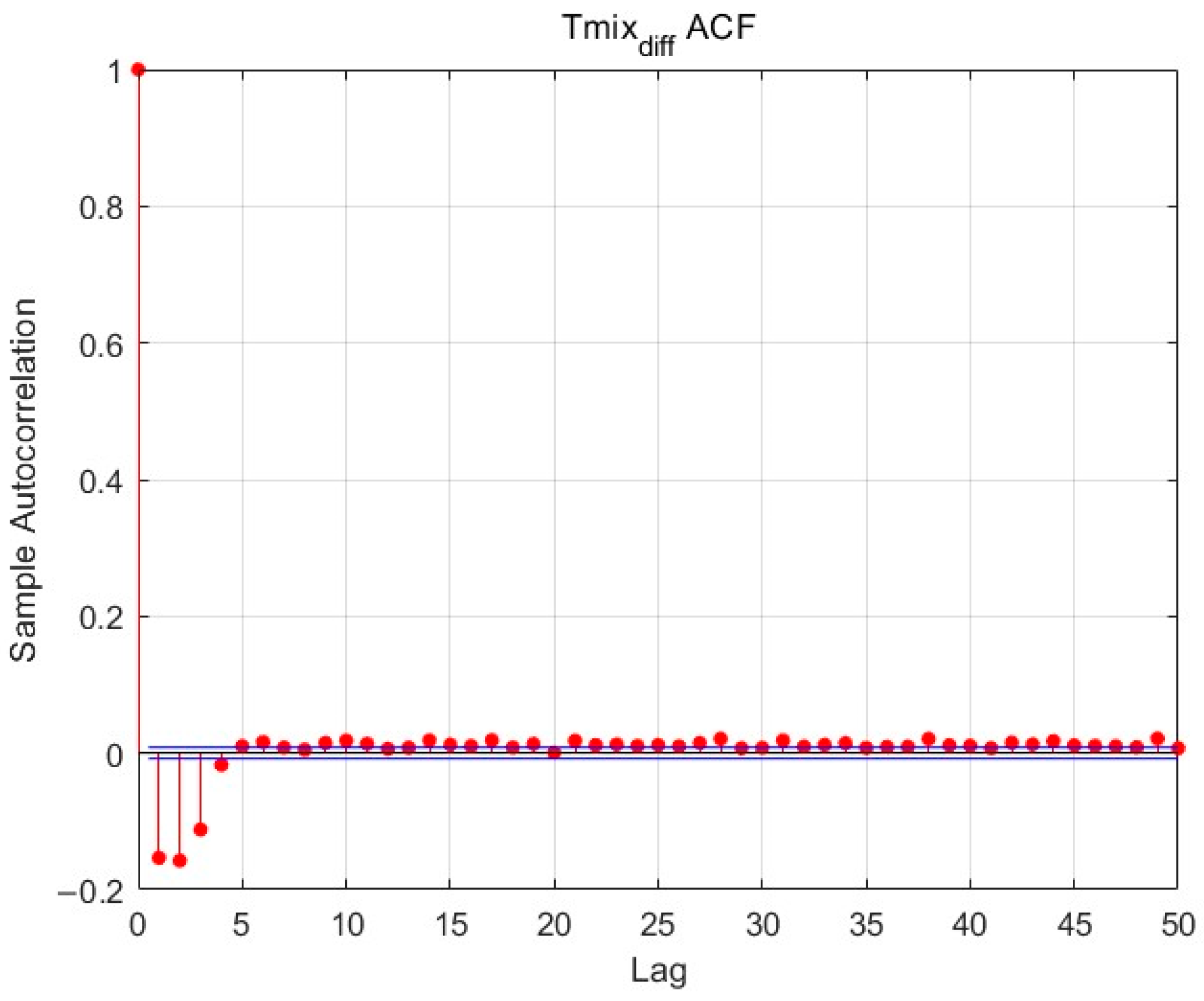
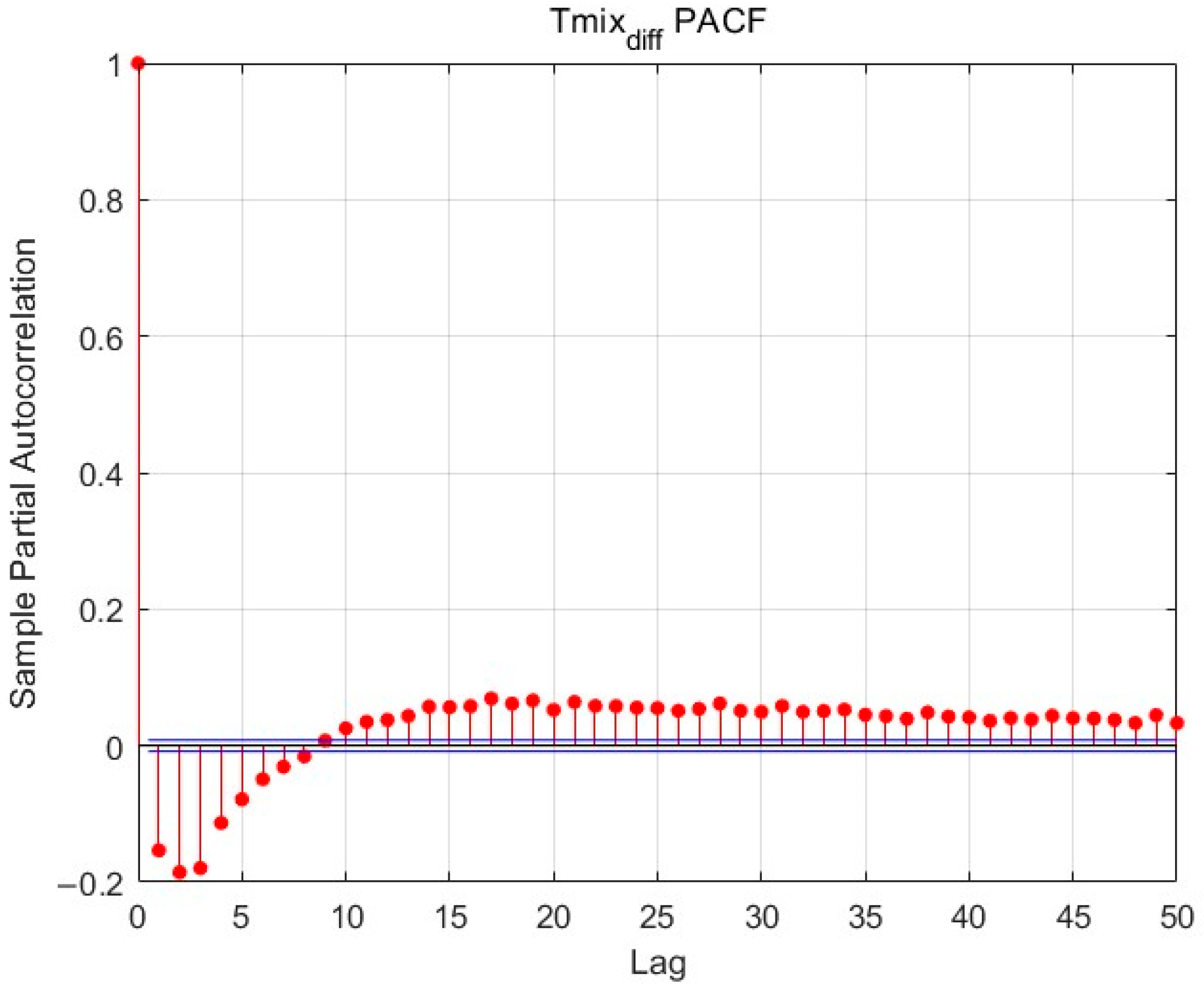
After differencing the outlet temperature $T_{mix}$, its ACF and PACF were computed, and the resulting correlation plots are shown in Figure 2 and Figure 3. The blue lines indicate the approximate 95% confidence intervals under the null hypothesis of white noise. Spikes exceeding these bounds suggest statistically significant correlations at the corresponding lags. The red vertical line at lag zero serves as a reference axis, distinguishing negative from positive lags. Analysis of the ACF and PACF reveals that the PACF at lag 1 deviates significantly from zero, indicating a strong linear correlation between the differenced temperature and its previous time step. Lags 2 to 5 show slight but noticeable significance, suggesting a certain degree of short-term negative feedback in the sequence. Beyond lag 5, the partial autocorrelations fall within the confidence bounds, indicating weak long-lag effects. Therefore, the differenced $T_{mix}$ series can be regarded as a short-memory process, mainly relying on the values from the previous five time steps.

3.2.3. Lag Response Analysis

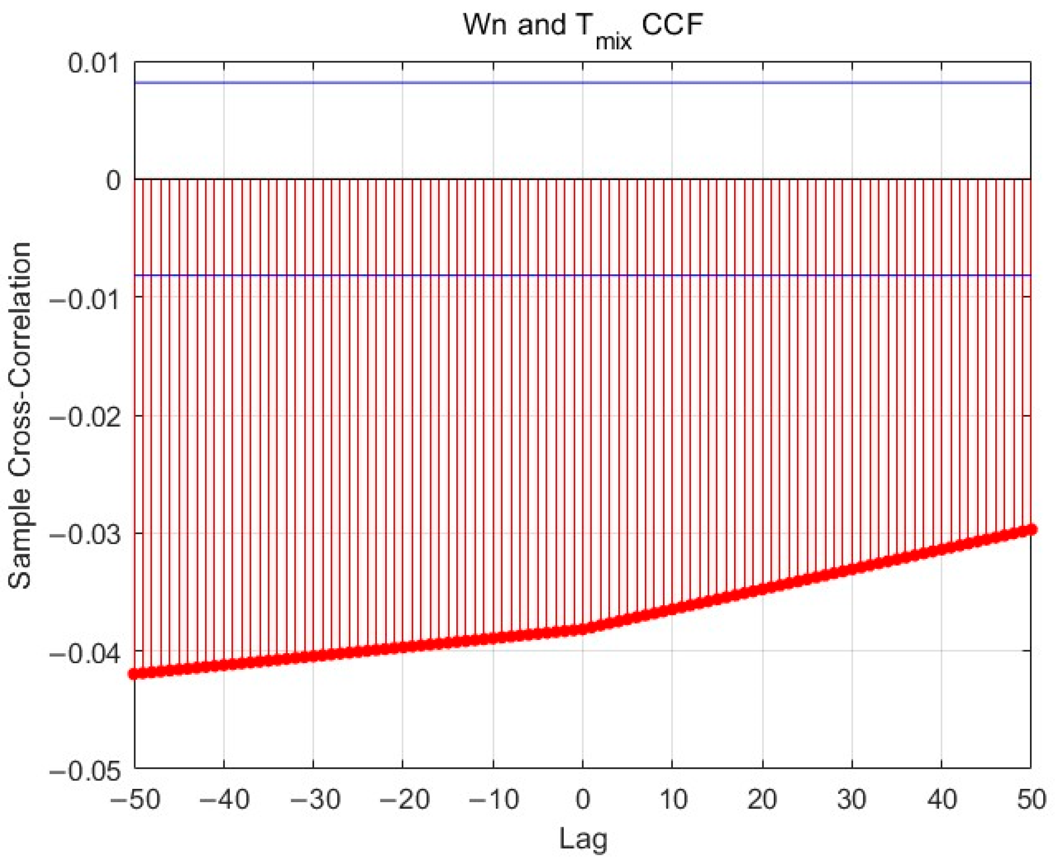
To investigate the dynamic influence of different air source flow rates on the mixer outlet temperature $T_{mix}$ this study calculates the Cross-Correlation Function (CCF) between cold air flow $W_c$ and ambient air flow $W_n$ with $T_{mix}$, with the maximum lag order set to 50. The results are shown in Figure 4 and Figure 5.

The analysis reveals a significant negative correlation between the $W_c$ and $T_{mix}$, indicating that an increase in $W_c$ leads to a reduction in $T_{mix}$, with a clear time-delay effect. In contrast, the correlation between $W_n$ and $T_{mix}$ is relatively weak, suggesting that $W_n$ has limited direct influence on outlet temperature variations. These observed lag characteristics reflect the inherent system inertia and energy accumulation effects, highlighting the necessity of incorporating temporal window mechanisms or recurrent structures into the prediction model to accurately capture the underlying dynamic behavior.

3.3. Physics Model with Inertia Process

The physical model derived from the energy conservation equation can be used for a rough estimation of the outlet temperature under ideal conditions. However, this theoretical formulation assumes perfect mixing and homogeneous thermal properties, which cannot fully represent the real system’s response latency and dynamic disturbances. To introduce these temporal characteristics, the system is modeled as a first-order inertia process:

$$\tau ·{\displaystyle \frac{{dT}_{cal\_delay}\left(t\right)}{dt}}+T_{cal\_delay}\left(t\right)=T_{cal}\left(t\right)$$

(12)

where $\tau$ is the time constant of the system, reflecting the degree of delay, $T_{cal}\left(t\right)$ is the instantaneous outlet temperature computed from the energy conservation model, and $T_{cal\_delay}\left(t\right)$ is the delayed (inertia-affected) outlet temperature.

By discretizing the differential equation using a forward Euler method, the model can be rewritten as:

$$T_{cal\_delay}\left(t+∆t\right)=T_{cal\_delay}\left(t\right)+{\displaystyle \frac{∆t}{\tau }}\left[{T_{cal}\left(t\right)-T}_{cal\_delay}\left(t\right)\right]$$

(13)

where $∆t$ is the sampling interval.

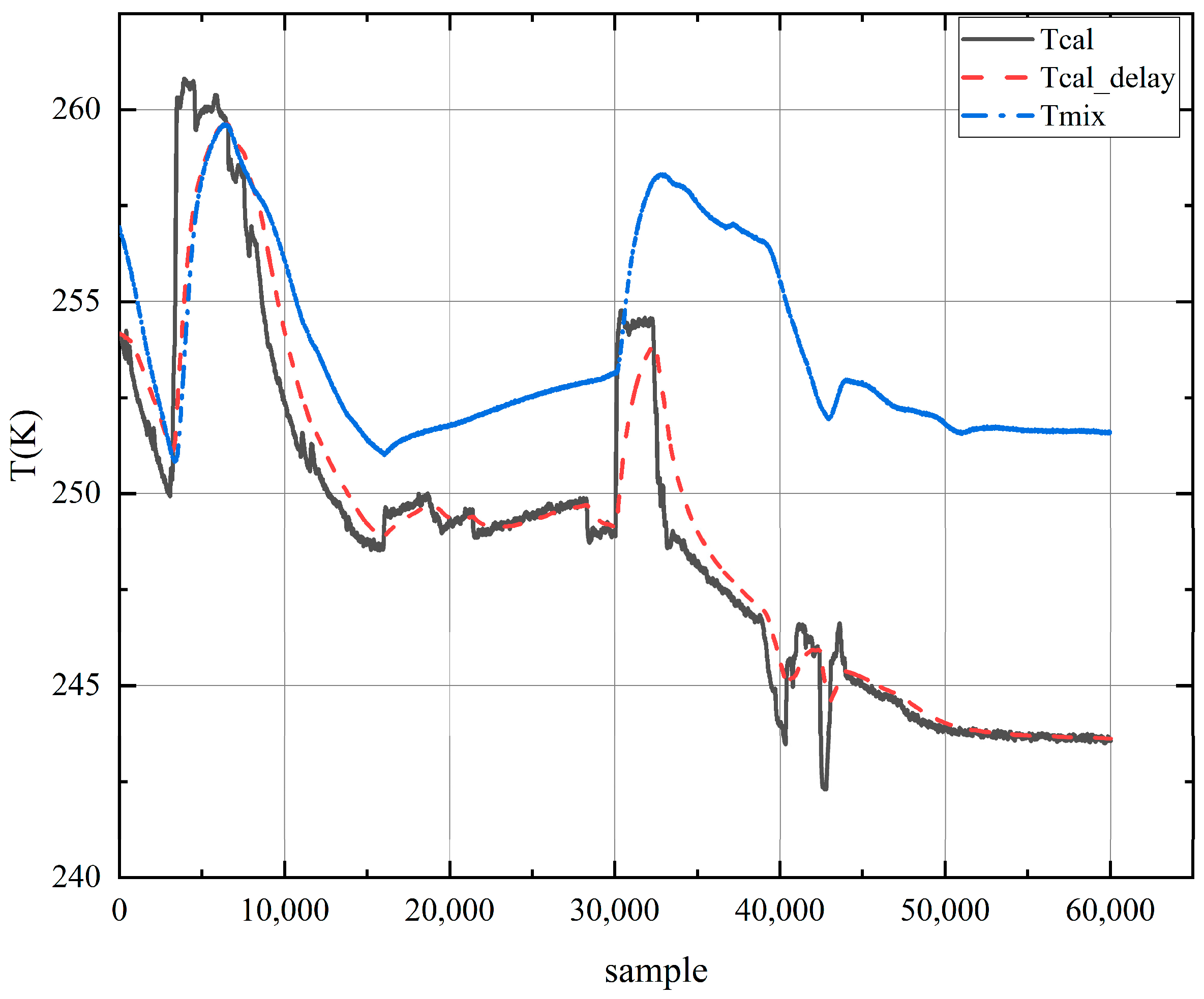
Figure 6 compares the actual outlet temperature, the theoretical prediction from the ideal physical model, and the output of the inertia-based model. The results demonstrate that the ideal model $T_{cal}$ responds rapidly to input perturbations but shows large deviations from the actual temperature trend. In contrast, introducing the inertial term $T_{cal\_delay}$ effectively smooths the model response and enhances its ability to capture gradual trends. However, the inertia-based model still exhibits limitations in tracking rapid fluctuations or complex nonlinear disturbances.

4. Methodology

To achieve high-precision and interpretable modeling of the outlet temperature $T_{mix}$ in dynamic air-mixing systems, this study proposes a hybrid modeling framework. The method integrates physics-informed priors, multiscale feature extraction, and a perturbation-aware dual-path memory structure to capture both the global trends and local disturbances in time-series data. This chapter elaborates on each component of the framework.

4.1. Physics-Guided Hybrid Modeling

The outlet temperature of an air mixer is fundamentally determined by the mixing enthalpy balance between two inlet airflows. The theoretical outlet temperature $T_{cal}$ can be derived via energy conservation principles, as introduced in Section 3.1 (Equation (4)). However, in real-world applications, disturbances such as actuator delay, heat loss, turbulence, and sensor noise result in significant deviations between the theoretical value and the actual measured $T_{mix}$.

To reconcile physical interpretability with data-driven flexibility, we adopt a gray-box modeling strategy [26]. The final predicted temperature is expressed as:

$$T_{mix}\left(t\right)\approx T_{cal}\left(t\right)+f_{\theta }\left(x_t\right)+\epsilon$$

(14)

where $x_t$ denotes the historical input sequence (e.g., previous flow rates and temperatures), $f_{\theta }\left(·\right)$ is a neural network parameterized by $\theta$, trained to learn the residual between $T_{mix}$ and $T_{cal}$, and $\epsilon$ is the residual noise term.

In training, a physics-regularized loss function is adopted to enhance consistency with domain knowledge:

$${\mathcal{L}}_{total}\approx {\mathcal{L}}_{mse}\left(T_{pred}, T_{mix}\right)+\lambda ·{\mathcal{L}}_{phys}\left(T_{pred},T_{cal}\right)$$

(15)

where ${\mathcal{L}}_{phys}$ enforces consistency between the predicted output and the physical model, $\lambda$ is a hyperparameter to control the trade-off between data fitting and physical regularization.

To exploit the trend-consistency advantage of $T_{cal}$ while mitigating the risk of performance degradation due to over-constraining, we propose a trend-aware weak physical constraint in the loss formulation. The physical loss is defined as:

$${\mathcal{L}}_{phys}\left(T_{pred},T_{cal}\right)={\displaystyle \frac{1}{N}}\sum _{t=1}^N{\left({\displaystyle \frac{T_{pred}\left(t\right)-T_{cal}\left(t\right)}{T_{cal}\left(t\right)+\epsilon }}\right)}^2·mask\left(t\right)$$

(16)

where $\epsilon$ is a small constant (set to ${10}^{-6}$) to prevent division by zero, and $mask\left(t\right)$ is a dynamic weighting term designed to weaken the physical constraint when the theoretical temperature is deemed unreliable.

The mask term is given by:

$$mask\left(t\right)=exp\left(-{\displaystyle \frac{\left|T_{cal}\left(t\right)-T_{cal}\left(t-1\right)\right|}{k}}\right)$$

(17)

where $k$ is a decay-rate hyperparameter. This formulation draws inspiration from adaptive weighting strategies in physics-informed neural networks [27], in which the balance between data loss and physical residual minimization is dynamically tuned to handle noisy or partially inaccurate physical models. In this paper, $mask\left(t\right)$ decays exponentially when large fluctuations occur in $T_{cal}$, signaling potential unreliability in the theoretical model under unstable operating conditions. This mechanism allows the hybrid model to fully leverage the theoretical trend information in stable regimes while relaxing the constraint when the physical model is less trustworthy.

4.2. Discrete Wavelet Transform (DWT)

Given that the outlet temperature reflects both global trends (e.g., flow regulation) and local disturbances (e.g., sharp flow changes), traditional LSTM or single-layer convolutional model is insufficient to capture these features [28]. Traditional time–domain or frequency–domain analysis methods struggle to effectively capture such complex temporal features. To address this limitation, DWT is introduced into the modeling process.

DWT is a powerful tool for time–frequency analysis, which decomposes a signal into different frequency bands with preserved temporal localization. Unlike the Fourier transform, which only provides frequency information, wavelet transform retains both time and scale (frequency) details, making it particularly suitable for analyzing non-stationary signals such as temperature and flow rate fluctuations.

Raw temperature and flow signals are decomposed into low- and high-frequency components using wavelet transform, allowing the model to separately capture global trends and local fluctuations:

$$x\left(t\right)=A\left(t\right)+D_1\left(t\right)+D_2\left(t\right)+\cdots$$

(18)

where $A\left(t\right)$ represents the smooth trend (low-frequency), and $D_i\left(t\right)$ are high-frequency perturbations. These components are then concatenated across channels to enhance robustness under dynamic conditions. This multi-resolution input significantly improves the model’s adaptability to non-stationary disturbances.

4.3. Perturbation-Aware Memory Structure

The temperature system typically exhibits slow-varying or lagging behavior, meaning that the effects of an upstream disturbance (e.g., a sudden change in airflow rate) may not immediately manifest at the outlet temperature. Instead, such perturbations propagate through the physical system over time, leading to a causal delay between input changes and output response. Capturing this lagged dependency is essential for improving multi-step prediction accuracy and system interpretability.

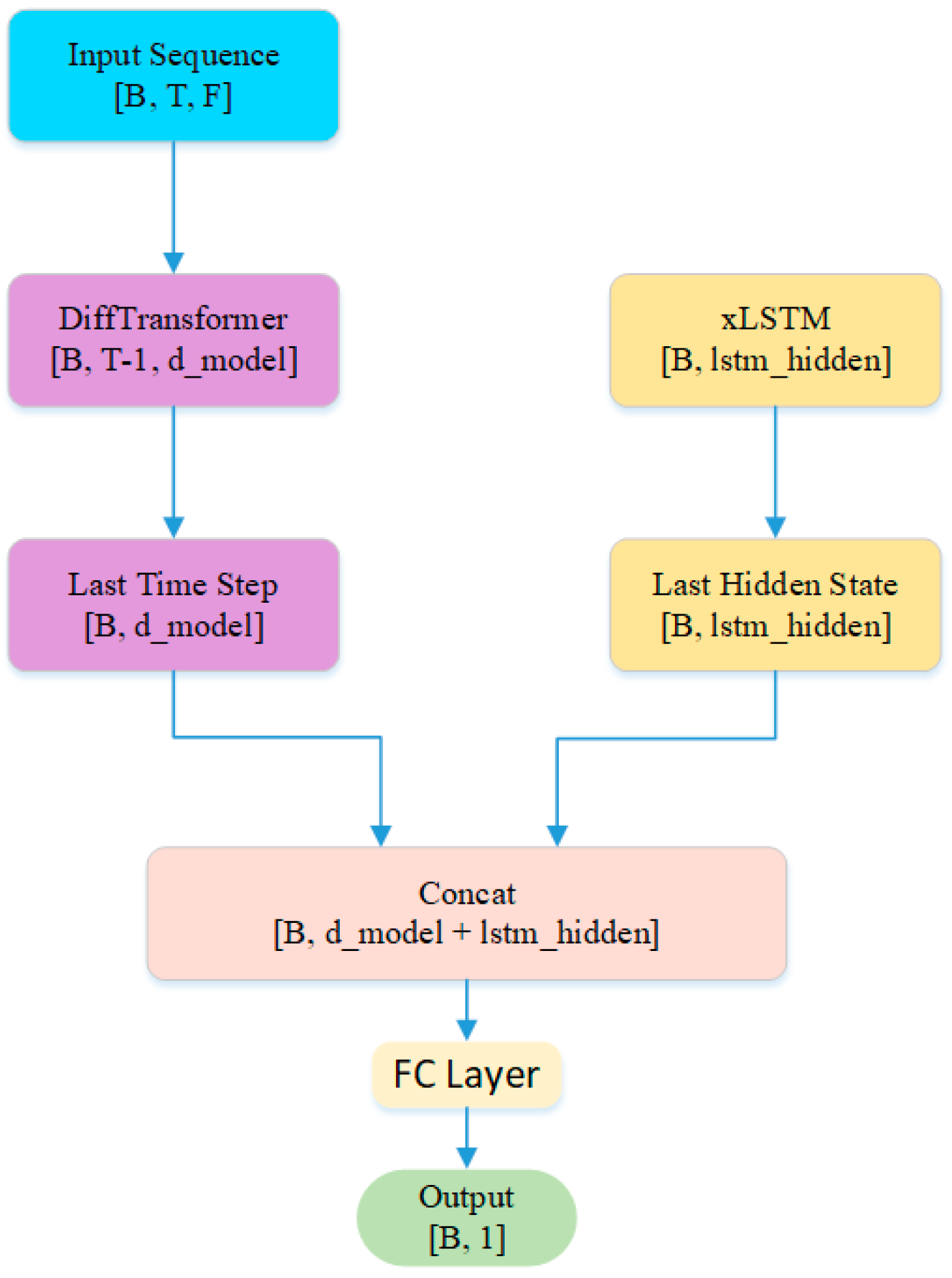
This work proposes a perturbation-aware memory structure that leverages dual-path temporal decomposition, integrating a decomposed Transformer path for long-term dependency modeling and an Extended Long Short-Term Memory (xLSTM) path for local short-term dynamics. Notably, the Transformer pathway processes the first-order differences of the input features, allowing the model to focus on temporal variations indicative of system perturbations. This hybrid design enhances both predictive accuracy and interpretability under dynamic input conditions.

4.3.1. Transformer for Long-Term Dependency Modeling

Compared to traditional Recurrent Neural Networks (RNNs), the Transformer model does not rely on sequential order. Instead, it captures dependencies among elements in the sequence through a self-attention mechanism. The core components of the Transformer model are the multi-head self-attention mechanism and a position-wise feedforward neural network. Through the multi-head attention mechanism, the model can automatically identify which historical inputs (e.g., sudden flow fluctuations) are more relevant to the current output. The attention weights provide interpretability regarding the causal origin of disturbances.

The self-attention mechanism takes as input a query matrix $Q$, a key matrix $K$, and a value matrix $V$, and computes the output as [29]:

$$Attention\left(Q,K,V\right)=softmax\left({\displaystyle \frac{Q{K}^T}{\sqrt{d_k}}}\right)V$$

(19)

where $d_k$ is the dimensionality of the key vectors, $1/\sqrt{d_k}$ is a scaling factor used to prevent the dot-product from becoming excessively large, and $softmax$ denotes the normalized exponential function.

The multi-head self-attention mechanism computes multiple self-attention operations in parallel, allowing the model to capture dependencies across different subspaces of the sequence. The output is obtained by concatenating the results from each attention head:

$$\left\{\begin{array}{c}Multihead\left(Q,K,V\right)=Concat\left({head}_1,\cdots ,{head}_h\right)W^o\\ {head}_i=Attention\left(Q{W}_i^Q,K{W}_i^K,V{W}_i^V\right)\end{array}\right.$$

(20)

where $W_i^Q$, $W_i^K$, $W_i^V$, and $W^o$ are learnable projection matrices for the query, key, value, and output, respectively.

The multi-head self-attention mechanism enables the model to identify which historical inputs (e.g., sudden flow changes) are most relevant to the current output. The attention weights provide interpretable insights into the causal origin of perturbations.

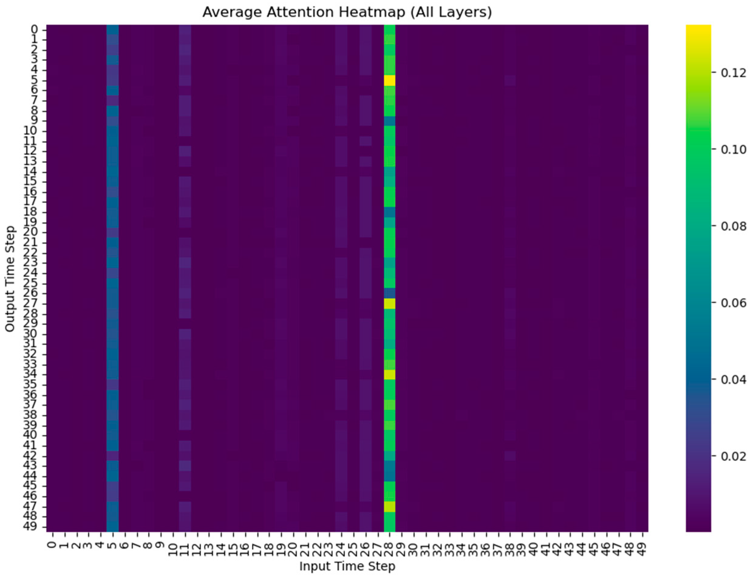
Figure 7 shows the average attention heatmap across all Transformer layers. The model predominantly attends to input time steps 8 and 36 when predicting the mixed temperature, indicating that these time points are the most informative for the output. This demonstrates that the model can identify and focus on the critical features, supporting its interpretability.

4.3.2. xLSTM for Short-Term Disturbance Sensitivity

To complement the long-term modeling capability of the Transformer, we introduce an xLSTM module that enhances sensitivity to short-term fluctuations and local nonlinear dynamics.

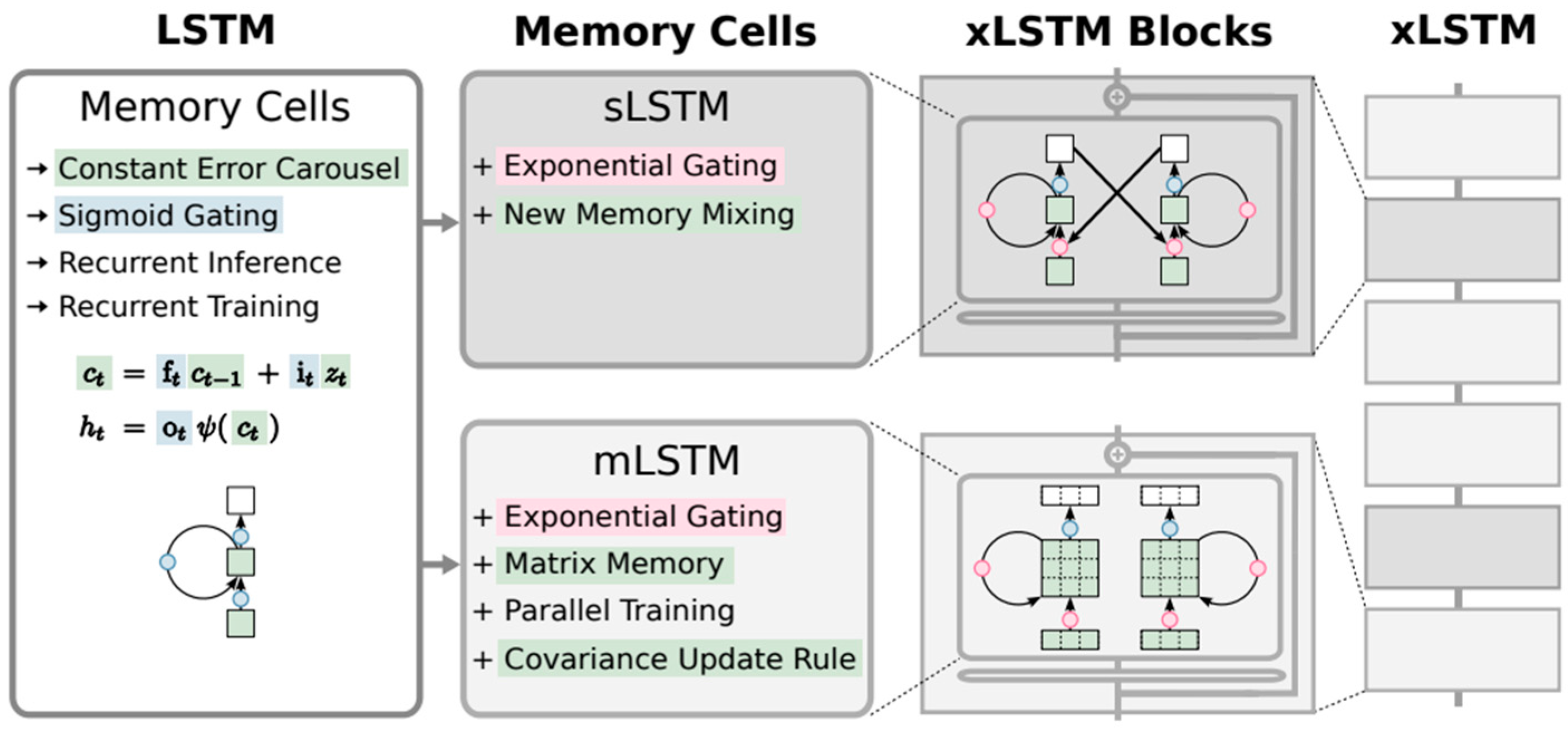
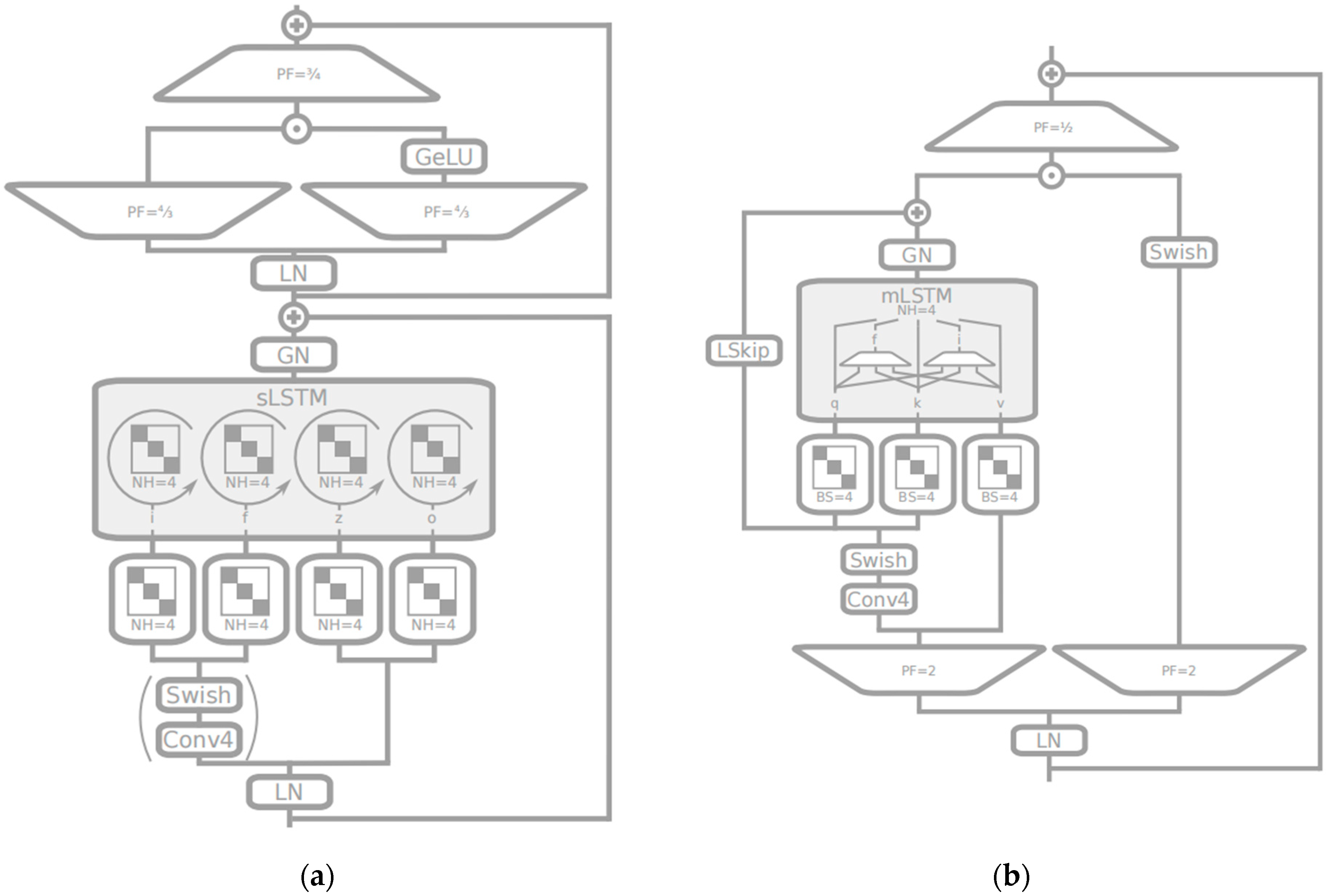
Compared to conventional LSTM, xLSTM introduces several key enhancements, including residual connections, layer-wise memory fusion, and gate-modulated memory updates. These modifications allow xLSTM to better capture fine-grained transient dynamics in time series while maintaining numerical stability during multistep predictions. Consequently, xLSTM provides superior capability in modeling complex nonlinear temporal dependencies and achieves higher predictive accuracy than standard LSTM models. The architecture of xLSTM is shown in Figure 8 [30], where its key submodules, sLSTM and mLSTM, are illustrated in are illustrated in Figure 9 [30].

4.3.3. Hybrid Integration and Perturbation-Aware Loss

The outputs from the Transformer and xLSTM branches are fused using a learnable gating or attention fusion layer. This enables the model to dynamically blend long-term memory with recent context.

To further prioritize disturbance periods, we design a perturbation-weighted loss that emphasizes prediction accuracy during abnormal intervals:

$${\mathcal{L}}_{p-aware}=\sum _t\omega \left(t\right)·{‖T_{pred}\left(t\right)-T_{mix}\left(t\right)‖}^2$$

(21)

where the weight $\omega \left(t\right)$ is derived from the temporal gradient (e.g., first-order derivative of flow rate or temperature). Larger weights are assigned during high-variance or critical control phases.

The final hybrid model integrates all the above modules, as shown in Figure 10.

To improve clarity and readability, a functional diagram of the fusion layer is provided, illustrating how the outputs from the Transformer and xLSTM branches are combined. Figure 11 demonstrates that the fusion layer first aligns the feature dimensions of both branches and then integrates them using a weighted combination, allowing the model to leverage both the temporal dependencies captured by the xLSTM and the long-range contextual information captured by the Transformer. This design enhances the overall predictive capability by effectively merging complementary information from the two branches.

5. Results and Discussion

5.1. Experimental Setup

5.1.1. Dataset and Operating Environment

To validate the effectiveness of the proposed hybrid modeling framework, we conduct a series of experiments based on the dataset sourced from real data collected during a high-altitude engine test for a specific model of aero-engine at a test site in Qingdao. The raw dataset is preprocessed to form a time-series dataset containing 60,000 samples with a time interval of 0.2 s. All model training and simulation experiments in this work were carried out on a laptop equipped with a Windows 11 operating system, Intel i7-12700H processor, 16G RAM, Python 3.9, and PyTorch 2.6.0+cu126.

5.1.2. Evaluation Metrics

The prediction evaluation metrics include the mean absolute error (MAE), root mean squared error (RMSE), mean absolute percentage error (MAPE) and coefficient of determination ($R^2$), calculated as Equations (15)–(17), respectively.

$$\mathrm{M}\mathrm{A}\mathrm{E}={\displaystyle \frac{1}{N}}\sum _{i=1}^N\left|y_i-{\widehat{y}}_i\right|$$

(22)

$$\mathrm{R}\mathrm{M}\mathrm{S}\mathrm{E}=\sqrt{{\displaystyle \frac{1}{N}}\sum _{i=1}^N{\left(y_i-{\widehat{y}}_i\right)}^2}$$

(23)

$$\mathrm{M}\mathrm{A}\mathrm{P}\mathrm{E}={\displaystyle \frac{1}{N}}\sum _{i=1}^N\left|{\displaystyle \frac{y_i-{\widehat{y}}_i}{y_i}}\right|\times 100\mathrm{\%}$$

(24)

$$R^2=1-{\displaystyle \frac{\frac{1}{N}\sum _{i=1}^N{\left(y_i-{\widehat{y}}_i\right)}^2}{\sum _{i=1}^N{\left(y_i-\frac{1}{N}\sum _{i=1}^N{y}_i\right)}^2}}$$

(25)

where ${\mathit{y}}_{\mathit{i}}$ and ${\widehat{\mathit{y}}}_{\mathit{i}}$ represent the actual and predicted values at time $\mathit{i}$, respectively, and $\mathit{N}$ is the number of samples. MAE and RMSE represent the absolute prediction errors. whereas MAPE reflects the relative magnitude of the prediction error with respect to the actual values, Lower values of MAE, RMSE, and MAPE indicate higher prediction accuracy. R² measures the goodness of fit of the model, with values closer to 1 indicating stronger predictive performance and better alignment with the observed data.

5.2. Experimental Results and Analysis

5.2.1. Performance Evaluation of the Prediction Model

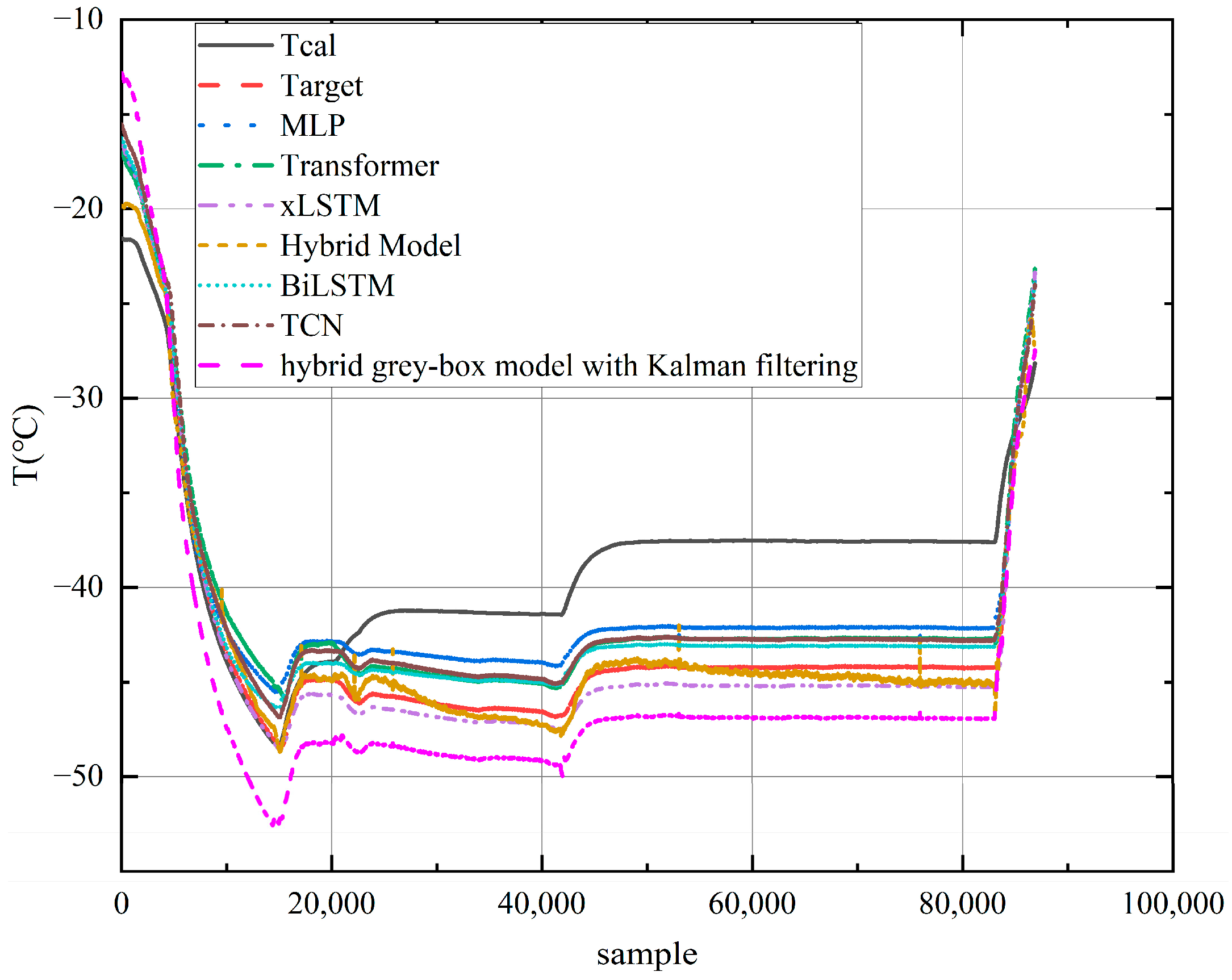
As shown in Figure 12 and

Table 3. Comparative evaluation of the proposed model and baseline models.

Comparative Models	Evaluation Metrics
	RMSE	MAE	MAPE	${\mathbf{R}}^2$
physics-only model	5.2445	4.6958	0.1109	0.3471
xLSTM	0.7721	0.7040	0.0159	0.9856
Transformer	1.5738	1.5046	0.0343	0.9401
MLP	2.0920	1.9455	0.0433	0.8942
hybrid grey-box model with Kalman filtering	2.8381	2.7645	0.0669	0.8053
BiLSTM	1.1802	1.0961	0.0248	0.9663
TCN	1.5031	1.4683	0.0344	0.9454
Hybrid Model	0.7414	0.5651	0.0156	0.9867

, it can be observed that the physics-only model shows the lowest performance across all metrics, which is expected due to its simplified assumptions. Data-driven models such as xLSTM, BiLSTM, and Transformer significantly improve the prediction accuracy, with R² values above 0.94. Among them, the xLSTM achieves relatively good results with RMSE = 0.7721.

The proposed Hybrid Model outperforms all baselines, achieving the lowest error values and the highest coefficient of determination, with the best results highlighted in bold. The detailed hyper-parameter configuration of all models is provided in Appendix A.

These results clearly demonstrate that the integration of multi-scale features and physical constraints within the Hybrid Model framework effectively improves outlet temperature prediction performance, providing a reliable solution for practical engineering applications.

5.2.2. Wavelet Ablation Study

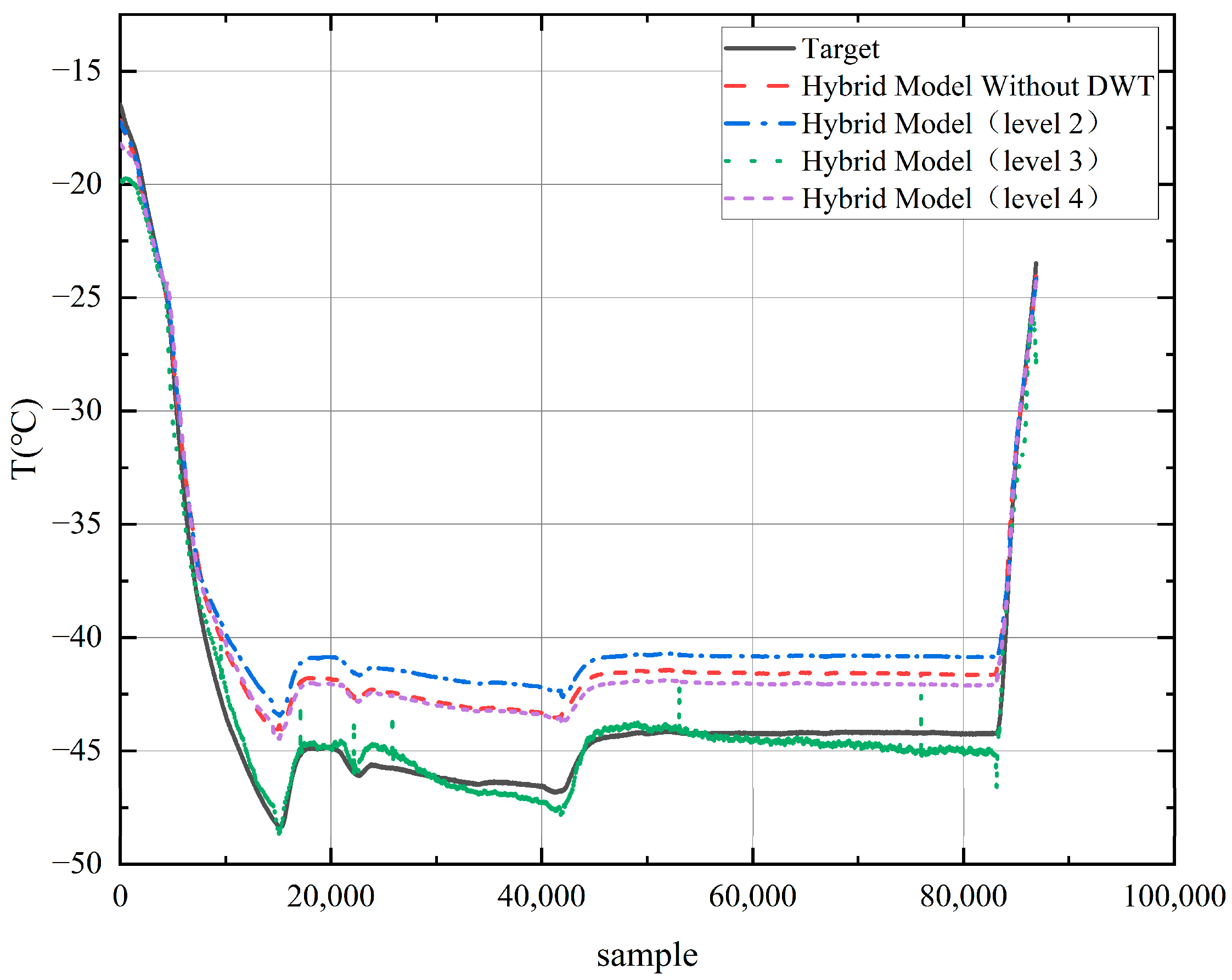
To verify the applicability of DWT for temperature sequences, this section conducts a wavelet ablation study to compare the prediction performance of the hybrid model.

Figure 13 and

Table 4. Comparative evaluation of the wavelet ablation study.

Comparative Models	Evaluation Metrics
	RMSE	MAE	MAPE	${\mathbf{R}}^2$
Hybrid Model (level 2)	3.6093	3.4126	0.0766	0.6852
Hybrid Model (level 3)	0.7414	0.5651	0.0156	0.9867
Hybrid Model (level 4)	2.5644	2.4258	0.0552	0.8411
Hybrid Model Without DWT	2.8025	2.6708	0.0603	0.8102

investigate the impact of DWT and different decomposition levels on the prediction performance of the proposed Hybrid Model. The results clearly indicate that introducing DWT significantly enhances model accuracy, while the choice of decomposition level plays a crucial role in determining the final performance.

Among the tested configurations, the Hybrid Model with level 3 decomposition achieves the best overall results, with the lowest RMSE, MAE, and MAPE, as well as the highest ${\mathrm{R}}^2$. This highlights that level 3 decomposition effectively balances the extraction of global trends and local fluctuations, providing optimal multi-scale feature representation for the model.

The Hybrid Model without DWT demonstrates the poorest performance among all DWT-enhanced models, confirming that incorporating wavelet-based multi-scale features is essential for accurately capturing complex, non-stationary characteristics in the outlet temperature sequence.

5.2.3. Ablation Study on Physical Constraint

To assess the contribution of the physical constraint module, a comparative experiment was conducted between the full hybrid model and a variant without the physics-informed loss term. As shown in

Table 5. Ablation study on the physical constraint module.

Comparative Models	Evaluation Metrics
	RMSE	MAE	MAPE	${\mathbf{R}}^2$
Hybrid Model	0.7414	0.5651	0.0156	0.9867
Hybrid Model Without Physical Constraint	1.8806	1.7655	0.0416	0.9145

, the inclusion of physical constraint significantly improves model performance across all evaluation metrics:

These results indicate that the physics-informed regularization not only reduces prediction error but also enhances model generalization and consistency with physical laws. The constraint acts as a soft prior that guides the model toward more physically plausible predictions, especially under conditions with limited or noisy data. This validates the effectiveness of integrating domain knowledge into data-driven architectures.

6. Conclusions

In this study, a hybrid mixer outlet temperature prediction method incorporating physical constraints and multiscale feature decomposition was proposed. The method effectively combines mechanistic modeling and advanced deep learning techniques to enhance prediction accuracy and robustness under complex conditions. Specifically, a theoretical outlet temperature was calculated based on mass and energy conservation principles, serving as a physical constraint to improve the model’s consistency with real-world thermodynamic behavior. Furthermore, DWT was employed to decompose raw time series into low- and high-frequency components, allowing the model to capture both global trends and local fluctuations.

A hybrid deep learning framework based on a difference-enhanced Transformer and xLSTM architecture was constructed to extract multi-scale temporal dependencies. Extensive experiments, including ablation studies and comparisons with baseline models, demonstrate that the proposed method significantly outperforms traditional machine learning and standard deep learning models in terms of prediction accuracy, generalization, and physical interpretability.

This research provides a practical and reliable approach for temperature prediction in a flight environment simulation intake system. Future work will focus on extending the method to multi-source airflow mixing scenarios and exploring adaptive physical parameter identification to further enhance model generalization capabilities.

Although the proposed model demonstrates excellent predictive accuracy on the current dataset, the data was collected from a single aero-engine and a specific experimental setup. The model’s performance under different engine types, operating conditions, or geometrical configurations may vary. Future work will investigate transfer learning and domain adaptation strategies to enhance generalizability across diverse engine architectures.

References

- Avril, A.; Hornung, C.H.; Urban, A.; Fraser, D.; Horne, M.; Veder, J.-P.; Tsanaktsidis, J.; Rodopoulos, T.; Henry, C.; Gunasegaram, D.R. Continuous flow hydrogenations using novel catalytic static mixers inside a tubular reactor. React. Chem. Eng. 2017, 2, 180–188. [Google Scholar] [CrossRef]
- Park, H.; Bach, C.K. A literature review of air mixing devices for psychrometric performance measurement applications (ASHRAE RP-1733). Sci. Technol. Built Environ. 2020, 26, 778–789. [Google Scholar] [CrossRef]
- Pei, X.; Zhang, S.; Dan, Z.; Zhu, M.; Qian, Q.; Wang, X. Study on digital modeling and simulation of altitude test facility flight environment simulation system. J. Propuls. Technol. 2019, 40, 1144–1152. [Google Scholar] [CrossRef]
- Zhu, M.; Wang, X.; Pei, X.; Zhang, S.; Dan, Z.; Miao, K.; Liu, J.; Jiang, Z. Multi-volume fluid-solid heat transfer modeling for flight environment simulation system. J. Propuls. Technol. 2020, 41, 2848–2859. [Google Scholar] [CrossRef]
- Wu, X. Research on Flow Characteristics and Structural Improvement of Engine Transition Test Mixer. Master’s Thesis, Southwest University of Science and Technology, Mianyang, China, 2024. [Google Scholar] [CrossRef]
- Huang, J.; Ming, P.; Sun, W. Dynamic modal analysis of fluid sweeping rods bundle. J. Eng. Thermophys. 2023, 44, 2279–2284. [Google Scholar]
- Zhang, P.; Li, Y.; Cheng, R. Control of Corner Separation for a Linear Compressor Cascade via Bionic Slanting Riblets at the Endwall. J. Therm. Sci. 2024, 34, 129–144. [Google Scholar] [CrossRef]
- Bagheri, A.; Patrignani, A.; Ghanbarian, B.; Pourkargar, D.B. A hybrid time series and physics-informed machine learning framework to predict soil water content. Eng. Appl. Artif. Intell. 2025, 144, 110105. [Google Scholar] [CrossRef]
- Naeini, S.S.; Snaiki, R. A physics-informed machine learning model for time-dependent wave runup prediction. Ocean Eng. 2024, 295, 116986. [Google Scholar] [CrossRef]
- Zhu, M.; Wang, X. An Integral Type Synthesis Method for Temperature and Pressure Control of Flight Environment Simulation Volume. In Proceedings of the ASME Turbo Expo 2017: Turbomachinery Technical Conference and Exposition, Charlotte, NC, USA, 26–30 June 2017. [Google Scholar]
- Wang, J.; Li, J.; Gao, Z.; He, X.; Zou, S.; Wan, J. Numerical simulation of internal flow field and structure improvement of hot air mixer. Chin. J. Process Eng. 2020, 20, 148–157. [Google Scholar]
- Zhu, J.; Dong, W.; Wu, F.; Tian, X. Calculation and analysis of heat transfer process in pipes of altitude test facility. Gas Turbine Exp. Res. 2011, 24, 10–14+24. [Google Scholar]
- Montgomery, P.; Burdette, R.; Klepper, J.; Milhoan, A. Evolution of a Turbine Engine Test Facility to Meet the Test Needs of Future Aircraft Systems. In Proceedings of the American Society of Mechanical Engineers(ASME) Turbo Expo 2002 v.1: Aircraft Engine Coal, Biomass, and Alternative Fuels Combustion and Fuels Education Electric Power Vehicular and Small Turbomachines, Amsterdam, The Netherlands, 1 December 2002; pp. 119–128. [Google Scholar]
- Montgomery, P.A.; Burdette, R.; Wilhite, L.; Salita, S. Modernization of a Turbine Engine Test Facility Utilizing a Real-Time Facility Model and Simulation. In Proceedings of the ASME TURBO EXPO 2001: Power for Land, Sea, & Air, New Orleans, LA, USA, 4–7 June 2001; pp. 4474–4481. [Google Scholar]
- Zhu, D. Structural Optimization Design of Cold and Hot Airflow Mixing Chamber. Master’s Thesis, Huazhong University of Science and Technology, Wuhan, China, 2022. [Google Scholar] [CrossRef]
- Hajirahimi, Z.; Khashei, M. Hybrid structures in time series modeling and forecasting: A review. Eng. Appl. Artif. Intell. 2019, 86, 83–106. [Google Scholar] [CrossRef]
- Wang, L.; Wang, Z.; Qu, H.; Liu, S. Optimal Forecast Combination Based on Neural Networks for Time Series Forecasting. Appl. Soft Comput. 2018, 66, 1–17. [Google Scholar] [CrossRef]
- Ning, Z.; Liu, X.; Wang, S. A digital twin modeling approach for aerospace control systems with mechanism and data fusion. Aerosp. Control Appl. 2022, 48, 1–7. [Google Scholar]
- Peng, L. Soft Measurement of Temperature in Vacuum Sintering Furnace Based on Mechanism and Data-Driven Hybrid Modeling. Master’s Thesis, Guangdong University of Technology, Guangzhou, China, 2020. [Google Scholar] [CrossRef]
- Yu, G. Research on Neural Network Predictive Control of Decomposing Furnace Outlet Temperature. Master’s Thesis, Hefei University of Technology, Hefei, China, 2021. [Google Scholar] [CrossRef]
- Kula, A.; Dąbrowski, D.; Blachnik, M.; Sajkowski, M.; Smalcerz, A.; Kamiński, Z. Modelling the Temperature of a Data Centre Cooling System Using Machine Learning Methods. Energies 2025, 18, 2581. [Google Scholar] [CrossRef]
- Zhang, Y.; Tian, Q.; Bai, Y. Prediction of Outlet Temperature of Circulating Water Based on Hybrid Model and Stacking Framework. Comput. Simul. 2023, 40, 172–177. [Google Scholar]
- Yan, L.; Lei, D.; Li, X.; Xu, L.; Dong, J.; Wang, Z. Outlet Temperature Prediction of Parabolic Trough Solar Field Based on Hybrid Neural Network. Acta Energiae Solaris Sin. 2023, 44, 265–273. [Google Scholar]
- Wang, J.; Tang, W.; Lv, T.; Ding, N. Simulation theory and methods of pipeline networks. Liaoning Chem. Ind. 2013, 42, 1476–1478. [Google Scholar]
- Elliott, G.; Rothenberg, T.J.; Stock, J.H. Efficient Tests for an Autoregressive Unit Root. Econometrica 1996, 64, 813–836. [Google Scholar] [CrossRef]
- Jagtap, A.D.; Kawaguchi, K.; Karniadakis, G.E. Adaptive activation functions accelerate convergence in deep and physics-informed neural networks. J. Comput. Phys. 2020, 404, 109136. [Google Scholar] [CrossRef]
- Raissi, M.; Perdikaris, P.; Karniadakis, G.E. Physics-informed neural networks: A deep learning framework for solving forward and inverse problems involving nonlinear partial differential equations. J. Comput. Phys. 2019, 378, 686–707. [Google Scholar] [CrossRef]
- Chen, H.; Ren, B. A multivariate time series forecasting model based on time-frequency feature fusion. J. Huazhong Univ. Sci. Technol. 2025, 1–13. [Google Scholar] [CrossRef]
- Vaswani, A.; Shazeer, N.; Parmar, N.; Uszkoreit, J.; Jones, L.; Gomez, A.N.; Kaiser, L.; Polosukhin, I. Attention Is All You Need. arXiv 2023, arXiv:1706.03762. [Google Scholar] [CrossRef]
- Beck, M.; Pöppel, K.; Spanring, M.; Auer, A.; Prudnikova, O.; Kopp, M.; Klambauer, G.; Brandstetter, J.; Hochreiter, S. xLSTM: Extended Long Short-Term Memory. arXiv 2024, arXiv:2405.04517. [Google Scholar] [CrossRef]