Article

A Direct Discrete Recurrent Neural Network with Integral Noise Tolerance and Fuzzy Integral Parameters for Discrete Time-Varying Matrix Problem Solving

1
School of Cyber Security, Guangdong Polytechnic Normal University, Guangzhou 510630, China
2
School of Information Engineering, Jiangxi University of Science and Technology, Ganzhou 341000, China
*
Author to whom correspondence should be addressed.
Symmetry 2025, 17(8), 1359; https://doi.org/10.3390/sym17081359
Submission received: 12 July 2025 / Revised: 10 August 2025 / Accepted: 16 August 2025 / Published: 20 August 2025
(This article belongs to the Section Mathematics)

Abstract

Discrete time-varying matrix problems are prevalent in scientific and engineering fields, and their efficient solution remains a key research objective. Existing direct discrete recurrent neural network models exhibit limitations in noise resistance and are prone to accuracy degradation in complex noise environments. To overcome these deficiencies, this paper proposes a fuzzy integral direct discrete recurrent neural network (FITDRNN) model. The FITDRNN model incorporates an integral term to counteract noise interference and employs a fuzzy logic system for dynamic adjustment of the integral parameter magnitude, thereby further enhancing its noise resistance. Theoretical analysis, combined with numerical experiments and robotic arm trajectory tracking experiments, verifies the convergence and noise resistance of the proposed FITDRNN model.

1. Introduction

Time-varying matrix problems are prevalent in mathematics [1,2], robotic motion control [3,4,5], image processing [6,7], and other fields. Their unique properties and computational complexity have attracted significant research attention. As a subfield, discrete time-varying matrix problems are also highly significant. Consequently, developing faster and more accurate solution methods for these discrete problems has become a key research objective. Symmetry analysis [8] often offers a pathway for simplifying such problems. For example, symmetric matrices leverage their symmetric structure to streamline operations like eigenvalue decomposition and matrix inversion [9]. Therefore, analyzing the symmetry or asymmetry of these matrices proves essential for enhancing algorithmic efficiency in solving discrete time-varying problems.
Discrete time-varying matrix problems in engineering applications frequently exhibit asymmetric structures due to dynamic properties and environmental noise interference [10]. This asymmetry presents dual challenges for model design: ensuring convergence and maintaining robustness. Recurrent neural networks (RNNs) demonstrate strong potential for resolving such dynamic problems by virtue of their excellent nonlinear mapping characteristics [11,12,13], providing innovative solutions to such problems. For instance, Shi et al. [14] proposed four novel discrete-time RNN (DT-RNN) models and verified the effectiveness of these DT-RNN models in solving such problems through numerical experiments. However, most existing discrete RNN models are obtained using indirect discretization methods. These approaches discretize the derived continuous models using established discretization techniques [15,16,17,18]. For instance, Yang et al. [18] applied a second-level discretization method to a continuous ZNN model, yielding Second-Level-Discrete Zeroing Neural Network (SLDZNN). These methods rely on a continuous-time framework, exhibiting computational complexity and limited efficiency [19].
To address the above limitations, Shi et al. [20] proposed a Taylor-based direct discretization method. This method first clarifies the target problem of discretization, then defines the error function for the discrete problem, processes the error function using Taylor expansion, derives the iterative update formula of the discrete-time RNN, and thereby constructs a direct discrete-time model to solve the corresponding discrete problem. Unlike traditional methods that first establish continuous time-varying models before discretization [21], the Taylor-based framework directly solves problems within the discrete-time paradigm [22]. This approach enhances computational efficiency and improves practical utility in engineering applications.
However, models developed using Taylor-based direct discretization methods are typically designed for ideal noise-free environments. In practical applications involving discrete time-varying matrix problems, noise interference is widespread, not only inducing computational errors but also compromising model stability [23]. Consequently, incorporating anti-noise mechanisms into model design is essential to overcome performance limitations in noisy environments and enhance adaptability to complex real-world scenarios. Currently, research on the noise resistance of direct discretization models remains limited. This contrasts with significant advances in noise-resistant modeling for continuous time-varying matrix problems solved via indirect discretization, where numerous effective models exist [24,25,26,27]. For example, Liu et al. [28] proposed a generalized RNN-based polynomial noise resistance (RB-PNR) model, which was verified through numerical simulations and robotic application experiments to effectively suppress polynomial noise. Similarly, Han et al. [29] constructed a triple-integral noise-resistant RNN (TINR-RNN) model, enabling the UR5 manipulator to track butterfly-shaped trajectories under noise interference and effectively suppress constant, linear, and polynomial noises. Inspired by these continuous domain approaches, this paper employed error accumulation in discrete time-varying matrix problems as an integral term to counteract noise interference.
Static mechanisms with fixed parameters exhibit inherent limitations: Their inability to perform real-time adjustments or adaptive optimizations in response to noise’s time-varying characteristics induces persistent parameter–environment mismatch. This misalignment impedes adaptation to complex, variable environments [30,31]. To enhance noise interference resistance, this research incorporated a fuzzy logic system. First proposed by Zadeh in 1965 [32], fuzzy set theory has experienced rapid development in industrial and control domains since its inception, owing to its remarkable capability to handle uncertainty and imprecision [33,34]. By emulating human decision-making processes, fuzzy systems effectively process imprecise information to address both fuzziness and dynamic changes in complex systems. As an important extension of fuzzy set theory, fuzzy logic systems are not only suitable for complex nonlinear systems but also exhibit certain anti-interference capabilities. Recent research has successfully integrated fuzzy logic systems into RNN architectures [35,36,37] to achieve dynamic adjustment of key parameters. For instance, Qiu et al. [37] adaptively regulated the step-size parameter of a discrete RNN model using a fuzzy control system and validated the effectiveness of the fuzzy logic system through numerical experiments.
The preceding analysis reveals two fundamental limitations of current direct discrete models: inadequate noise tolerance and static parameterization. To address these challenges, this paper proposes a fuzzy integral direct discrete recurrent neural network (FITDRNN) model, developed through direct discretization principles. Specifically, targeting the common noise interference in practical applications, the model incorporates an error accumulation integral term during its construction to enhance the inherent noise suppression capability and improve the basic anti-interference performance of the model. Meanwhile, it integrates a fuzzy logic system to dynamically adjust the integral parameters of the model, enabling the model to perceive noise changes in real time and adaptively update parameters. As a result, the robustness and convergence speed of the model are enhanced. The key contributions of this paper are outlined below.
  • The FITDRNN model is proposed based on the direct discretization concept. By integrating the dynamic modeling capability of the RNN and the parameter adaptive adjustment mechanism of the fuzzy logic system, it specifically addresses the defects of insufficient noise resistance and parameter staticity in existing direct discretization models, significantly improving the robustness and solution accuracy of the model in noisy environments.
  • It strictly proves the robustness and convergence characteristics of the FITDRNN model in both noise-free and noisy scenarios, establishing theoretical foundations for its practical application.
  • Numerical experiments confirm FITDRNN’s efficacy in solving discrete time-varying matrix problems while maintaining exponential error convergence amid diverse noise interference, exhibiting superior convergence and robustness.
  • Applied to robotic arm trajectory tracking, the model achieves precise tracking under noise-free and noisy environments, validating its utility in actual control systems.
The remainder of this paper is organized as follows: In Section 2, the mathematical formulation of discrete time-varying matrix problems is expounded, and the design process of the FITDRNN model is introduced in detail. Section 3 focuses on the fuzzy logic system adopted by the FITDRNN model, presenting its design details. Section 4 theoretically analyzes the convergence and robustness of the FITDRNN model. Section 5 conducts simulation experiments and presents the results. Section 6 discusses the limitations of the model and future directions for improvement. Finally, Section 7 summarizes and prospects the research contents of this paper.

2. Problem Formulation and Model Construction

This section first formulates the target discrete time-varying matrix problem. It then presents the mathematical formulations of the direct discrete recurrent neural network (TDRNN) model and adaptive direct-discretized recurrent neural network (ADD-RNN) model for solving this problem. The section concludes with a detailed description of the proposed fuzzy integral direct discrete recurrent neural network (FITDRNN) model.

2.1. Problem Formulation

The discrete time-varying matrix problem is described as:
Υ ( t h + 1 ) χ ( t h + 1 ) = Γ ( t h + 1 ) ,
where Υ ( t h + 1 ) R m × n denotes a full-rank dynamic coefficient matrix, Γ ( t h + 1 ) R m × n is a dynamic matrix, and χ ( t h + 1 ) R n × n denotes the unknown matrix to be solved within each time interval t h , t h + 1 0 , + . It is worth noting that in order to obtain the real-time value of χ ( t h + 1 ) , the previous and current values should be fully utilized.

2.2. TDRNN Model

First, Q ( χ ( t h + 1 ) , t h + 1 ) and Q ( χ ( t h ) , t h ) represent the error equations of Equation (1) at time t h + 1 and t h , respectively. Q ( χ ( t h + 1 ) , t h + 1 ) can be defined as follows:
Q ( χ ( t h + 1 ) , t h + 1 ) = Υ ( t h + 1 ) χ ( t h + 1 ) Γ ( t h + 1 ) .
The Taylor-based direct discretization method employs a second-order Taylor expansion [20]:
Q ( χ ( t h + 1 ) , t h + 1 ) = Q ( χ ( t h ) , t h ) + ( Q ( χ ( t h ) , t h ) / χ ( t h ) ) ( χ ( t h + 1 ) χ ( t h ) ) + ( d Q ( χ ( t h ) , t h ) / d t h ) ( t h + 1 t h ) + O ( τ 2 ) ) ,
where O ( τ 2 ) represents the higher-order infinitesimal term. Next, let Q ( χ ( t h + 1 ) , t h + 1 ) = ϖ Q ( χ ( t h ) , t h ) [20], where h is sufficiently large and ϖ is a design parameter. Building upon this formulation, a TDRNN model for addressing the discrete time-varying matrix problem (1) is thereby derived, with the formulation given below.
χ ( t h + 1 ) = ( ϖ 1 ) Υ ( t h ) 1 ( Υ ( t h ) χ ( t h ) Γ ( t h ) ) ε Υ ( t h ) 1 ( Υ ˙ ( t h ) χ ( t h ) Γ ˙ ( t h ) ) + χ ( t h ) ,
where ε = t h + 1 t h represents the sampling gap.

2.3. ADD-RNN Model

Building upon the design concept of the Taylor-based direct discretization method, Qiu et al. [38] utilized the formula Q ( χ ( t h + 1 ) , t h + 1 ) = ( 1 λ ) Q ( χ ( t h ) , t h ) to derive the direct discrete model as follows:
χ ( t h + 1 ) = λ Υ ( t h ) 1 ( Υ ( t h ) χ ( t h ) Γ ( t h ) ) ε Υ ( t h ) 1 ( Υ ˙ ( t h ) χ ( t h ) Γ ˙ ( t h ) ) + χ ( t h ) ,
where λ = 0.1 + ς denotes the fuzzy-enhanced solution step size. Furthermore, a fuzzy control system (FCS) is integrated into this model to enable adaptive adjustment of its parameter ς .

2.4. FITDRNN Model

First, the error function Q ( χ ( t h ) , t h ) of discrete time-varying matrix problem (1) can be defined as follows:
Q ( χ ( t h ) , t h ) = Υ ( t h ) χ ( t h ) Γ ( t h ) .
Utilizing the first-order Taylor expansion formula [37], we have
Q ( χ ( t h + 1 ) , t h + 1 ) = Q ( χ ( t h ) , t h ) + ε Q ˙ ( χ ( t h ) , t h ) + O ( ε 2 ) .
Applying the chain rule, the time derivative Q ˙ ( χ ( t h ) , t h ) can be expressed as
Q ˙ ( χ ( t h ) , t h ) = Υ ( t h ) χ ˙ ( t h ) + ( Υ ˙ ( t h ) χ ( t h ) Γ ˙ ( t h ) ) ,
where χ ˙ ( t h ) can be expanded using the forward Euler method as
χ ˙ ( t h ) = χ ( t h + 1 ) χ ( t h ) ε .
Therefore, Equation (6) can be rewritten as
Q ( χ ( t h + 1 ) , t h + 1 ) = Q ( χ ( t h ) , t h ) + Υ ( t h ) ( χ ( t h + 1 ) χ ( t h ) ) + ε ( Υ ˙ ( t h ) χ ( t h ) Γ ˙ ( t h ) ) + O ( ε 2 ) .
When h tends to infinity, Q ( χ ( t h + 1 ) , t h + 1 ) = ϖ Q ( χ ( t h ) , t h ) ξ i = 0 h Q ( χ ( t i ) , t i ) is defined, where ϖ is a design parameter, and ξ denotes an integral parameter. It can be obtained that
Q ( χ ( t h + 1 ) , t h + 1 ) Q ( χ ( t h ) , t h ) = ( ϖ 1 ) Q ( χ ( t h ) , t h ) ξ i = 0 h Q ( χ ( t i ) , t i ) .
By combining Equations (7) and (8), we can derive
( ϖ 1 ) Q ( χ ( t h ) , t h ) ξ i = 0 h Q ( χ ( t i ) , t i ) = Q ( χ ( t h ) , t h ) + Υ ( t h ) ( χ ( t h + 1 ) χ ( t h ) ) + ε ( Υ ˙ ( t h ) χ ( t h ) Γ ˙ ( t h ) ) + O ( ε 2 ) .
Neglecting O ( ε 2 ) and substituting Equation (5) into (9) yields
( ϖ 1 ) ( Υ ( t h ) χ ( t h ) Γ ( t h ) ) ξ i = 0 h ( Υ ( t i ) χ ( t i ) Γ ( t i ) ) = Υ ( t h ) ( χ ( t h + 1 ) χ ( t h ) ) + ε ( Υ ˙ ( t h ) χ ( t h ) Γ ˙ ( t h ) ) .
By arranging the above expressions (10), we can obtain
χ ( t h + 1 ) = ( 1 ϖ ) Υ ( t h ) 1 ( Υ ( t h ) χ ( t h ) Γ ( t h ) ) ε Υ ( t h ) 1 ( Υ ˙ ( t h ) χ ( t h ) Γ ˙ ( t h ) ) ξ Υ ( t h ) 1 i = 0 h ( Υ ( t i ) χ ( t i ) Γ ( t i ) ) + χ ( t h ) .
Then, the fuzzy logic system is incorporated into Equation (11). The FITDRNN model can be expressed as
χ ( t h + 1 ) = ( 1 ϖ ) Υ ( t h ) 1 ( Υ ( t h ) χ ( t h ) Γ ( t h ) ) ε Υ ( t h ) 1 ( Υ ˙ ( t h ) χ ( t h ) Γ ˙ ( t h ) ) γ Υ ( t h ) 1 i = 0 h ( Υ ( t i ) χ ( t i ) Γ ( t i ) ) + χ ( t h ) ,
where γ = c α represents an adaptively adjusted fuzzy integral parameter that replaces the original fixed parameter ξ . Here, c denotes an arbitrary positive constant controlling the regulation amplitude of the integral term, while α functions as a fuzzy factor generated by the fuzzy logic system in Section 3. This factor dynamically adjusts γ through real-time output, constituting the core mechanism enabling γ ’s adaptive capability. In order to investigate the noise resilience of the FITDRNN model, an unknown noise term U ( t h ) is introduced. The above FITDRNN model can be rewritten as
χ ( t h + 1 ) = ( 1 ϖ ) Υ ( t h ) 1 ( Υ ( t h ) χ ( t h ) Γ ( t h ) ) ε Υ ( t h ) 1 ( Υ ˙ ( t h ) χ ( t h ) Γ ˙ ( t h ) ) γ Υ ( t h ) 1 i = 0 h ( Υ ( t i ) χ ( t i ) Γ ( t i ) ) + ε Υ ( t h ) 1 U ( t h ) + χ ( t h ) .

3. Fuzzy Logic System

This section presents the fuzzy logic system (FLS) that generates the fuzzy integral parameter for the proposed FITDRNN model (12). In general, constructing an FLS involves three steps, i.e., fuzzification, fuzzy inference engine, and defuzzification. By following these three steps, a fuzzy factor can be derived. Subsequently, the FLS is constructed in line with these three steps.
1.
Fuzzification
Fuzzification is the initial step in an FLS, converting precise input data into fuzzy sets using membership functions. In this paper, the residual error ρ = Υ ( t h ) χ ( t h ) Γ ( t h ) F was employed as input, where · denotes the Frobenius norm. The fuzzy input set is defined as M, and the fuzzy output set is defined as N. Both input and output membership functions utilize Gaussian functions [37], which are symmetric (i.e., axisymmetric) about their centers, as shown in Figure 1. The Gaussian membership function is defined as
υ ( x ) = e ( x a ) 2 2 ϱ 2 ,
where parameter a represents the center of Gaussian functions and ϱ controls the width.
2.
Fuzzy inference engine
The fuzzy inference engine forms the core of the FLS. It processes the fuzzified inputs by matching them against predefined fuzzy rules, determining the activation degrees of the rules based on this match, and calculating the membership degrees of the output variable in the fuzzy sets according to the rule activations. Fuzzy rules define the mapping relationships between input fuzzy sets M and output fuzzy sets N. Specifically, the FLS uses the following rules:
R 1 : if M = S then N = S ; R 2 : if M = M S then N = M S ; R 3 : if M = M L then N = M L ; R 4 : if M = L then N = L .
where S, M S , M L , and L represent small, medium-small, medium-large, and large, respectively.
3.
Defuzzification
Within an FLS, the fuzzy inference engine outputs the membership degrees of the output variable. Defuzzification converts this fuzzy output into a precise numerical value. Various defuzzification methods exist [39], including the largest of maximum, centroid, and bisector methods. This paper employed the centroid method. Among these, it used the centroid position of the output fuzzy set as the precise output value. The centroid method comprehensively considers the contributions of all activated fuzzy rules, providing a smooth output. It is defined as follows:
α = O α υ ( α ) d α O υ ( α ) d α ,
where α is the fuzzy factor, and O represents the domain of α .

4. Theoretical Analyses

This section conducts a rigorous theoretical analysis of the FITDRNN model, covering its convergence characteristics and noise robustness in the context of solving discrete time-varying linear matrix problems.
Theorem 1.
The proposed FITDRNN model (12) can be equivalently expressed as follows:
( 2 ϖ ) Q ( χ ( t h ) , t h ) = Q ( χ ( t h 1 ) , t h 1 ) γ i = 0 h Q ( χ ( t i ) , t i ) + ε U ( t h ) + O ( ε 2 ) .
Proof of Theorem 1.
Based on the Euler method, Υ ˙ ( t h ) and Γ ˙ ( t h ) can be formulated as
Υ ˙ ( t h ) = Υ ( t h ) Υ ( t h 1 ) ε ,
Γ ˙ ( t h ) = Γ ( t h ) Γ ( t h 1 ) ε .
Expanding χ ( t h + 1 ) and χ ( t h ) using Taylor formula [38] yields
χ ( t h + 1 ) = χ ( t h ) + ε χ ˙ ( t h ) + O ( ε 2 ) ,
and
χ ( t h ) = χ ( t h 1 ) + ε χ ˙ ( t h ) + O ( ε 2 ) .
Substituting the expressions Υ ˙ ( t h ) , Γ ˙ ( t h ) , χ ( t h ) and χ ( t h + 1 ) into the FITDRNN model (12) yields
χ ( t h ) + ε χ ˙ ( t h ) = ( 1 ϖ ) Υ ( t h ) 1 Q ( χ ( t h ) , t h ) ε Υ ( t h ) 1 ( Υ ( t h ) Υ ( t h 1 ) ε ( χ ( t h 1 ) + ε χ ˙ ( t h ) ) Γ ( t h ) Γ ( t h 1 ) ε ) γ Υ ( t h ) 1 i = 0 h Q ( χ ( t i ) , t i ) + ε Υ ( t h ) 1 U ( t h ) + χ ( t h 1 ) + ε χ ˙ ( t h ) + O ( ε 2 ) ,
and simplifying the above Equation (15) yields the following:
( 2 ϖ ) Q ( χ ( t h ) , t h ) Q ( χ ( t h 1 ) , t h 1 ) + ε Υ ( t h ) χ ˙ ( t h ) = ε Υ ( t h 1 ) χ ˙ ( t h ) γ i = 0 h Q ( χ ( t i ) , t i ) + ε U ( t h ) + O ( ε 2 ) .
Substituting Formula (14) into Equation (16) again and simplifying it yields the following result:
( 2 ϖ ) Q ( χ ( t h ) , t h ) = Q ( χ ( t h 1 ) , t h 1 ) γ i = 0 h Q ( χ ( t i ) , t i ) + ε U ( t h ) + O ( ε 2 ) .
Theorem 2.
In the absence of noise, the steady-state residual lim h Q ( χ ( t h + 1 ) , t h + 1 ) 2 of the proposed FITDRNN model (12) is O ( ε 2 ) when h is large enough.
Proof of Theorem 2. 
Under noise-free conditions, i.e., U ( t h ) = 0 , Equation (13) can be denoted as
( 2 ϖ ) Q ( χ ( t h ) , t h ) = Q ( χ ( t h 1 ) , t h 1 ) γ i = 0 h Q ( χ ( t i ) , t i ) + O ( ε 2 ) .
Similarly, the equation at time t h + 1 can be derived. By subtracting Equation (17) at time t h from that at time t h + 1 , we have
( 2 ϖ + γ ) Q ( χ ( t h + 1 ) , t h + 1 ) = ( 3 ϖ ) Q ( χ ( t h ) , t h ) Q ( χ ( t h 1 ) , t h 1 ) + O ( ε 2 ) .
Let the m - th , m [ 1 , n ] subtracting of Q ( χ ( t h + 1 ) , t h + 1 ) be q ( t h + 1 ) m , then Equation (18) can be written as
( 2 ϖ + γ ) q ( t h + 1 ) m = ( 3 ϖ ) q ( t h ) m q ( t h 1 ) m + O ( ε 2 ) .
To perform stability analysis via eigenvalues [40], ϕ ( t h + 1 ) m = q ( t h + 1 ) m , q ( t h ) m T is defined. For the state-space equation corresponding to Equation (19), the control strategy is
ϕ ( t h + 1 ) m = N ϕ ( t h ) m + O ( ε 2 ) ,
where matrix N is expressed as follows:
N = 3 ϖ 2 ϖ + γ 1 2 ϖ + γ 1 0 .
Using the triangle inequality property of the norm, we have
| | ϕ ( t h + 1 ) m | | 2 | | N | | 2 | | ϕ ( t h ) m | | 2 + O ( ε 2 ) | | N | | 2 | | N ϕ ( t h 1 ) m | | 2 + | | N | | 2 O ( ε 2 ) + O ( ε 2 ) | | N | | 2 2 | | ϕ ( t h 1 ) m | | 2 + O ( ε 2 ) | | N | | 2 h | | ϕ ( t 1 ) m | | 2 + O ( ε 2 ) .
The absolute values of the real parts of the eigenvalues of matrix N are all less than 1; therefore, lim h N 2 h = 0 , and it follows that
lim h | | ϕ ( t h + 1 ) m | | 2 = O ( ε 2 ) .
According to ϕ ( t h + 1 ) m = e ( t h + 1 ) m , e ( t h ) m T , it can be derived that the steady-state residual lim h Q ( χ ( t h + 1 ) , t h + 1 ) 2 is O ( ε 2 ) . □
Theorem 3.
With interference from random bounded noise U ( t h ) = u ( t h ) , the steady-state residual lim h Q ( χ ( t h + 1 ) , t h + 1 ) 2 of the FITDRNN model (12) is bounded by 2 n sup 1 p h , 1 m n | u p m | / ( 1 N 2 ) + O ( ε 2 ) .
Proof of Theorem 3. 
Under random bounded noise disturbance, the equation of (13) can be expressed as
( 2 ϖ ) Q ( χ ( t h ) , t h ) = Q ( χ ( t h 1 ) , t h 1 ) γ i = 0 h Q ( χ ( t i ) , t i ) + ε u ( t h ) + O ( ε 2 ) .
Similar to the proof process of Theorem 2, let φ ( t h ) m = u ( t h ) m u ( t h 1 ) m , 0 T . The control strategy is
ϕ ( t h + 1 ) m = N ϕ ( t h ) m + φ ( t h ) m ,
then
| | ϕ ( t h + 1 ) m | | 2 | | N | | 2 | | ϕ ( t h ) m | | 2 + | | φ ( t h ) m | | 2 | | N | | 2 | | N ϕ ( t h 1 ) m | | 2 + | | N | | 2 | | φ ( t h 1 ) m | | 2 + | | φ ( t h ) m | | 2 | | N | | 2 h | | N ϕ ( t 1 ) m | | 2 + | | N | | 2 h 1 | | φ ( t 1 ) m | | 2 + + | | φ ( t h ) m | | 2 < | | N | | 2 h | | N ϕ ( t 1 ) m | | 2 + max 1 p h | | φ h m | | 2 / ( 1 | | N | | 2 ) < | | N | | 2 h | | N ϕ ( t 1 ) m | | 2 + 2 max 1 p h | u ( t h ) m | 2 / ( 1 | | N | | 2 ) .
According to Theorem 2, lim h N 2 h = 0 . It can be obtained that
lim h Q ( χ ( t h + 1 ) , t h + 1 ) 2 < 2 n sup 1 p h , 1 m n | u p m | / ( 1 N 2 ) + O ( ε 2 ) .
Theorem 4.
With constant noise interference, the steady-state residual lim h Q ( χ ( t h + 1 ) , t h + 1 ) 2 of the proposed FITDRNN model (12) is O ( ε 2 ) .
Proof of Theorem 4. 
Similar to Theorem 2, the Equation (13) subsystem with constant noise U ( t h ) = C is constructed as follows:
( 2 ϖ + γ ) q ( t h + 1 ) m = q ( t h ) m γ i = 0 h q ( t i ) + C m + O ( ε 2 ) ,
and application of the Z-transform yields
q z m = ( 2 ϖ + γ ) z ( z 1 ) q m + z C m ( 2 ϖ + γ ) z ( z 1 ) ( z 1 ) + z γ .
Then, by applying the properties of the final value theorem of the Z-transform, we have
lim h q h m = lim z 1 ( z 1 ) ( ( 2 ϖ + γ ) z ( z 1 ) q m + z C m ( 2 ϖ + γ ) z ( z 1 ) ( z 1 ) + z γ = 0 .
Through the above proof, it follows that the steady-state residual error is O ( ε 2 ) . The proof of the steady-state residual error under linear noise interference is the same as above, and will not be repeated. □

5. Numerical Simulation and Mechanical Arm Application

This section verifies the convergence characteristics and robustness of the proposed FITDRNN model (12) through a numerical simulation and a robotic arm trajectory tracking experiment.

5.1. Numerical Simulation

This subsection applies the FITDRNN model (12) to solve the following discrete time-varying matrix problem. The experiment utilized sample data derived from the mathematical essence of discrete time-varying matrix problems. The coefficient matrices Υ ( t h ) R 2 × 2 and Γ ( t h ) R 2 × 2 followed typical dynamic evolution forms in time-varying system theory [2,23], defined as
Υ ( t h ) = sin ( t h ) cos ( t h ) cos ( t h ) sin ( t h ) ,
and
Γ ( t h ) = sin ( 2 t h ) cos ( 2 t h ) cos ( 2 t h ) sin ( 2 t h ) .
To facilitate comparative analysis, the theoretical solution χ * ( t h ) expression is
χ * ( t h ) = Υ ( t h ) 1 Γ ( t h ) = cos ( t h ) sin ( t h ) sin ( t h ) cos ( t h ) .
In the numerical experiment, the sampling gap ε was set to 0.001. The convergence parameter ϖ for both the TDRNN model (3) and the FITDRNN model (12) was set to 0.7. The initial fuzzy-enhanced solution step size λ of the ADD-RNN model (4) was configured as 0.3, and the initial fuzzy integral parameter γ of the FITDRNN model (12) was set as 1. During online computation, the fuzzy integral parameter γ was dynamically generated by the FLS, while the fuzzy-enhanced solution step size λ was dynamically optimized by the FCS.
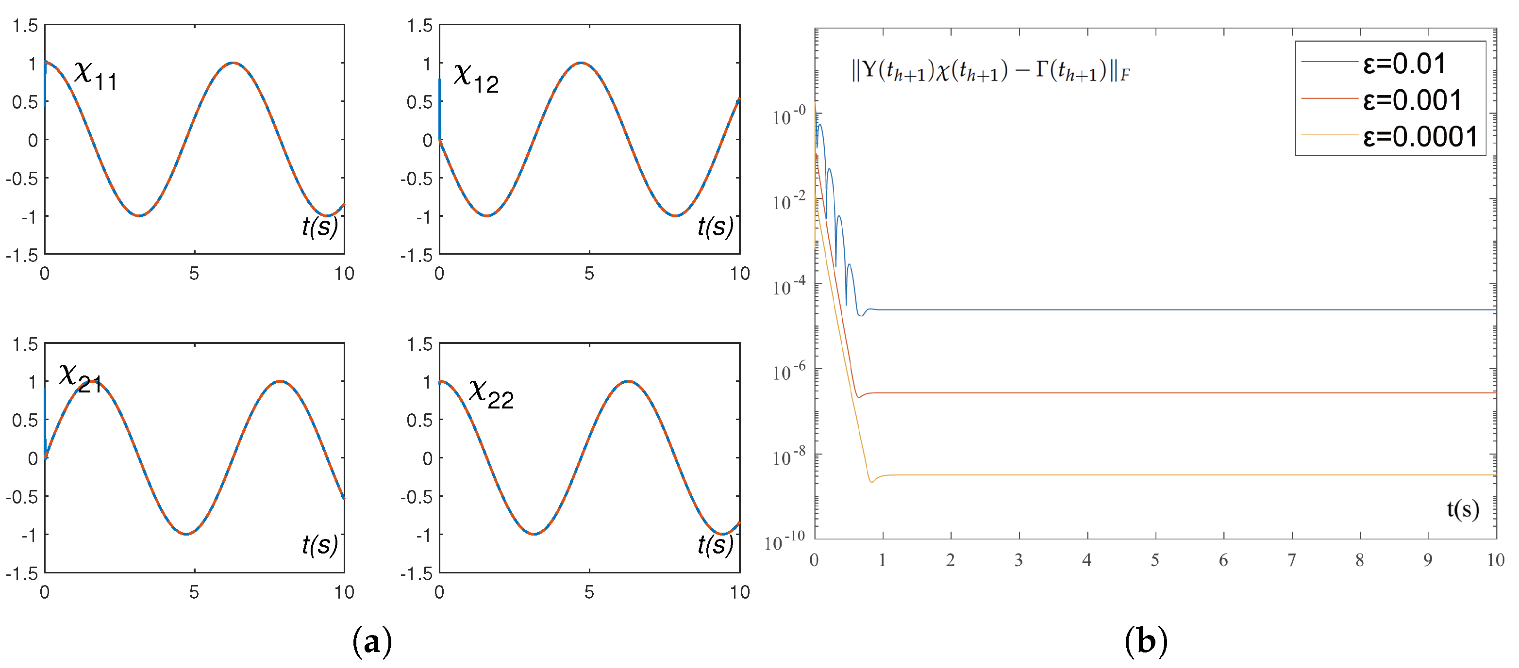
Under noise-free conditions, the FITDRNN model (12) was applied to solve the above-mentioned discrete time-varying matrix problem. The experimental results are clearly demonstrated in Figure 2 and Figure 3. Figure 2a presents the trajectories of the theoretical solution χ * ( t h ) and the state solution χ ( t h ) : The theoretical solution is marked by red dashed lines, while the state solution is represented by blue dashed lines. It can be observed that the state solution converged rapidly to the theoretical solution with random initial value. To further analyze how the sampling gap ε influences FITDRNN model (12) performance, Figure 2b illustrates the variation of the residual error of the FITDRNN model (12) under different values of ε . The experimental data show that when ε changed from 0.01 to 0.001, the residual error correspondingly varied from 10 5 to 10 7 . This demonstrates that the residual error of the FITDRNN model (12) varies in the form of O ( ε 2 ) , consistent with the theoretical analysis in Section 4. Figure 3 compares the residual errors of the TDRNN (3), ADD-RNN (4), and FITDRNN (12) models across varying ε values. The results demonstrate significantly smaller residual errors for the FITDRNN model (12) compared to both TDRNN (3) and ADD-RNN (4) across all tested ε values, confirming its superior convergence accuracy.
To validate its robustness in noisy environments, the FITDRNN model (12) was applied to solving the same discrete time-varying matrix problem in a noisy environment, with the TDRNN model (3) and the ADD-RNN model (4) introduced for comparison. Three noise types were tested: constant noise U ( t h ) = 50 , linear noise U ( t h ) = 50 + t h , and random bounded noise U ( t h ) [ 55 , 60 ] . The experimental results are presented in Figure 4 and Table 1. Specifically, in both constant and linear noise environments, the residual errors of both the TDRNN model (3) and the ADD-RNN model (4) stabilized at 10 1 , while the residual error of the FITDRNN model (12) was 10 8 —significantly lower than the residual errors of the former two models. Under random bounded noise, the ADD-RNN model (4) achieved a residual error of 10 2 , while the FITDRNN model (12) was 10 3 . Notably, the residual error of the ADD-RNN model (4) under random bounded noise was smaller than that under linear noise. This finding suggests that the FCS performs better at handling uncertainty. Based on the above conclusions, the FITDRNN model (12) exhibits superior noise resistance over the TDRNN model (3) and the ADD-RNN model (4) across different noise scenarios. To investigate the effect of the values of ε on the performance of the FITDRNN model (12) in noisy environments, the relevant experimental results are shown in Table 2. The experimental data demonstrate that regardless of the noise environment, the residual error of the FITDRNN model (12) varies in the form of O ( ε 2 ) . The results confirm the robustness of the proposed FITDRNN model (12).

5.2. Mechanical Arm Application

This section applies the FITDRNN model (12) to a manipulator trajectory tracking task, demonstrating its practical utility. For robotic arm trajectory tracking, the position and orientation of the end-effector in Cartesian space can be computed using the manipulator’s joint angles, and the mapping relationship between these variables is expressible as
Ψ ( β ( t h ) ) = f ( t h ) ,
where β ( t h ) represents the joint angle vector, and f ( t h ) denotes the end-effector position vector. Here, Ψ ( · ) is the kinematic mapping function that transforms the joint state into the position information of the end-effector. According to the literature [41], the Cartesian velocity of the end-effector f ˙ ( t h ) and the joint velocity β ˙ ( t h ) are related as follows:
J ( β ( t h ) ) β ˙ ( t h ) = f ˙ ( t h ) ,
where J ( β ( t h ) ) = Ψ ( β ( t h ) ) β ( t h ) denotes the Jacobian matrix. The target trajectory follows a standard flower-shaped path [42], commonly used in this field to evaluate robotic arm performance in complex curve tracking tasks. This trajectory is defined as
f ( t h ) = 1 4 cos π 5 t h 1 4 sin π 5 t h 1 5 sin π 2 t h .
The initial joint angle was set as β ( t 0 ) = 0 , π / 6 , 0 , π / 3 , 0 , π / 6 T , and the tracking task was configured to span 20 s. Meanwhile, the sampling gap ε , the design parameter ϖ , and the integral parameter γ maintained identical values to those in the numerical experiment.
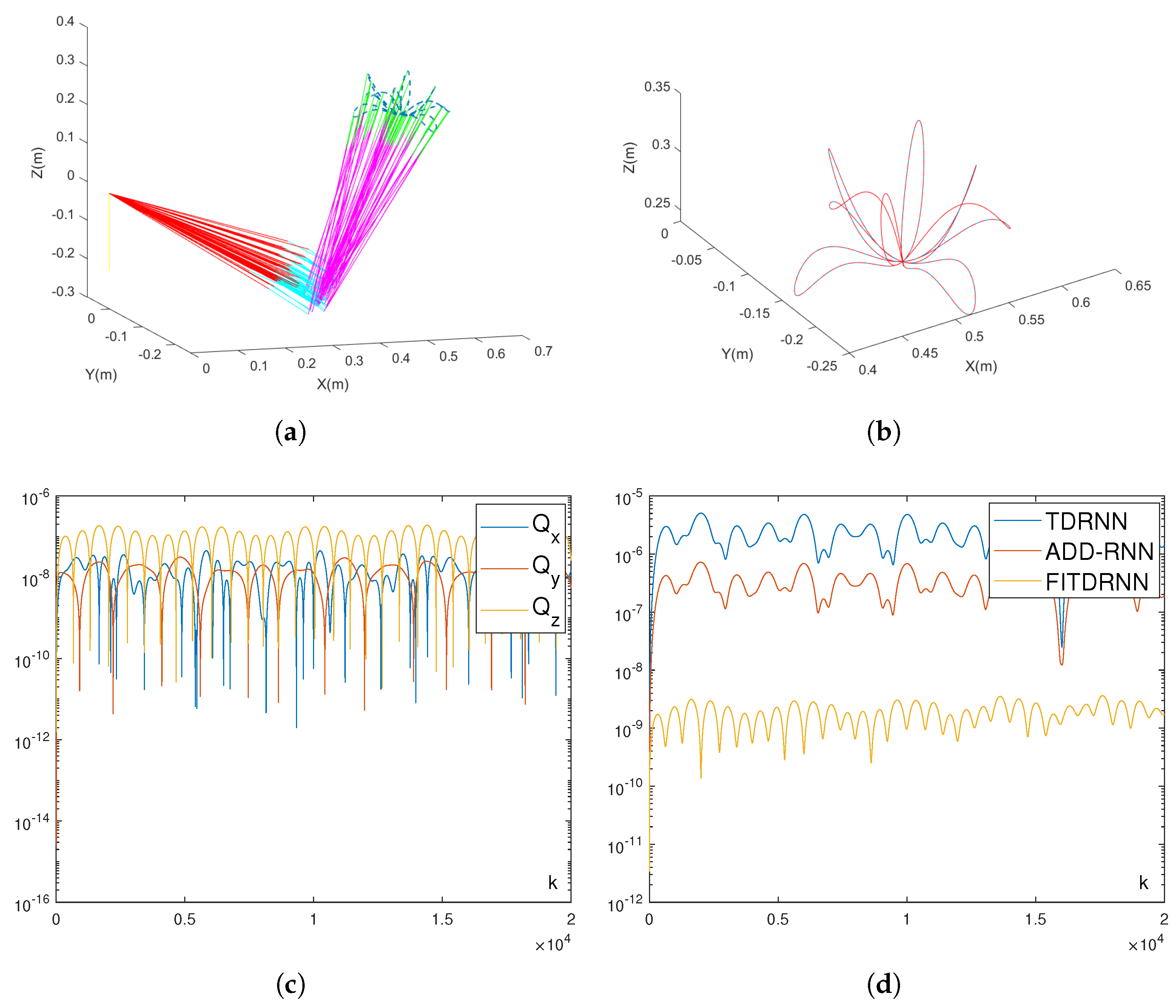
In the absence of noise, the experimental results are presented in Figure 5. Figure 5a displays the trajectory of the robotic arm during the tracking process, while Figure 5b depicts the actual and desired trajectories of the robot end-effector. It can be clearly observed that the trajectory presents an approximately rotationally symmetric feature around the center in three-dimensional space, and the actual trajectory aligns remarkably well with the desired trajectory, which indicates that the FITDRNN model (12) can successfully accomplish the robotic arm trajectory tracking task. Meanwhile, Figure 5c shows the error between the actual and desired trajectories of the X, Y, and Z axes of the robotic arm when it performed the tracking task. Figure 5d presents the error comparison among the TDRNN model (3), ADD-RNN model (4), and FITDRNN model (12). It is evident that the residual error of the TDRNN model (3) is 10 6 , the ADD-RNN model (4) is 10 7 , and the FITDRNN model (12) is 10 8 , with the error of the FITDRNN model (12) being significantly lower than that of the TDRNN model (3) and ADD-RNN model (4).
To validate the noise resistance of the FITDRNN model (12), this research introduced multiple types of noise interference and compared its performance with the TDRNN model (3) and the ADD-RNN model (4). Specifically, the experimental settings included an integral parameter set as 120 α , a constant noise intensity of 10, a linear noise intensity of 10 + h , and a random bounded noise of U ( t h ) [ 10 , 15 ) . Figure 6 presents the residual errors of the three models in different noise environments. The results demonstrate that under constant noise, the TDRNN model (3) failed to resist interference entirely, and the ADD-RNN model (4) exhibited moderate noise resistance, while the FITDRNN model (12) achieved complete noise suppression, with a residual error of 10 5 . When facing linear and random bounded noise, both the TDRNN model (3) and the ADD-RNN model (4) struggled to effectively counteract noise disturbances, whereas the FITDRNN model (12) maintained a residual error of 10 5 , demonstrating exceptional noise resistance. In summary, the FITDRNN model (12) significantly outperformed the TDRNN model (3) and the ADD-RNN model (4) across all noise scenarios, validating its effectiveness for practical applications in complex, noisy environments.

6. Discussion

While the proposed FITDRNN model effectively solved discrete time-varying matrix problems and demonstrated robust noise resistance, it still has certain limitations. The first limitation involves the inherent subjectivity in designing the fuzzy rule base. The model’s fuzzy logic system employs an empirically designed rule base, which inevitably introduces subjective bias. Although these rules performed well in our experimental scenarios, they may lack precision in specific application contexts. The second limitation involves elevated computational overhead. Although the integration of fuzzy logic enhances the model’s robustness, it simultaneously raises computational costs. This is particularly critical in time-sensitive applications (e.g., high-speed industrial control systems and millisecond-scale image processing), as the iterative process of fuzzy rule reasoning may cause system delays.
To address these constraints, future research will prioritize two key directions: The first research axis will focus on developing autonomous rule evolution mechanisms for fuzzy logic systems through data-driven methods, enabling self-optimizing rule generation to reduce empirical dependency and enhance model generalizability. The second axis will entail investigating lightweight iterative processes for fuzzy systems, aiming to significantly reduce computational latency while maintaining dynamic parameter optimization efficacy, ultimately enhancing adaptability to real-time industrial applications.

7. Conclusions

This paper presented a fuzzy integral direct discrete recurrent neural network (FITDRNN) model for solving discrete time-varying matrix problems. The model synergistically integrates integral-term processing into a fuzzy logic system (FLS) to achieve superior noise adaptability. Theoretical analysis rigorously established the convergence and robustness of the proposed model. Furthermore, numerical experiments quantitatively compared the residual errors among the TDRNN (3), ADD-RNN (4), and FITDRNN (12) models under noise interference, confirming the superior noise resistance of the FITDRNN model. Furthermore, the FITDRNN model (12) was successfully validated in robotic arm trajectory tracking tasks, demonstrating its practical utility.
The proposed model can achieve excellent scalability in large-scale complex scenarios via three core aspects: Architecturally, its modular structure, integrating the fuzzy logic parameter adjustment and integral anti-noise modules, enables computational power expansion on a parallel framework to efficiently handle high-dimensional discrete time-varying matrix problems. For anti-noise performance, the fuzzy logic system’s rule base has dynamic expandability. It flexibly adds adaptive rules based on scenario complexity, accurately capturing multi-source heterogeneous noise characteristics to mitigate interference. In implementation, the iterative update formula from Taylor-based direct discretization avoids redundant computations from continuous to discrete model conversions, ensuring efficiency. Notably, in robotic arm multi-joint control and high-dimensional image processing, the model maintains convergence efficiency and robustness through adaptive parameter optimization, supporting large-scale practical applications.

Author Contributions

Conceptualization, C.Y.; data curation, J.C.; formal analysis, J.C.; funding acquisition, C.Y.; investigation, J.C.; methodology, J.C.; project administration, C.Y.; resources, C.Y.; software, J.C.; supervision, C.Y.; validation, J.C.; visualization, J.C.; writing—original draft, J.C.; writing—review and editing, C.Y., J.C. and L.L. All authors have read and agreed to the published version of the manuscript.

Funding

This research was funded by the Special Projects in National Key Research and Development Program of China (2018YFB1802200), the GPNU Foundation (2022SDKYA029), the Key Areas of Guangdong Province (2019B010118001), and the National Natural Science Foundation of China (NSFC: 11561029).

Data Availability Statement

The original contributions presented in this study are included in the article material. Further inquiries can be directed to the corresponding author.

Conflicts of Interest

The authors declare no conflicts of interest.

References

  1. Gao, Y.; Tang, Z.; Ke, Y.; Stanimirovi, P. New Activation Functions and Zhangians In Zeroing Neural Network and Applications to Time-Varying Matrix Pseudoinversion. Math. Comput. Simul. 2024, 225, 1–12. [Google Scholar] [CrossRef]
  2. Chen, Y.; Chen, J.; Yi, C. A Pre-Defined Finite Time Neural Solver for The Time-Variant Matrix Equation E(t)X(t)G(t) = D(t). J. Frankl. Inst. 2024, 361, 106710. [Google Scholar] [CrossRef]
  3. Liao, B.; Wang, Y.; Li, J.; Guo, D.; He, Y. Harmonic Noise-Tolerant ZNN for Dynamic Matrix Pseudoinversion and Its Application to Robot Manipulator. Front. Neurorobot. 2022, 16, 928636. [Google Scholar] [CrossRef] [PubMed]
  4. Tang, W.; Cai, H.; Xiao, L.; He, Y.; Li, L.; Zuo, Q.; Li, J. A Predefined-Time Adaptive Zeroing Neural Network for Solving Time-Varying Linear Equations and Its Application to UR5 Robot. IEEE Trans. Neural Netw. Learn. Syst. 2025, 36, 4703–4712. [Google Scholar] [CrossRef] [PubMed]
  5. Li, C.; Zheng, B.; Ou, Q.; Wang, Q.; Yue, C.; Chen, L.; Zhang, Z.; Yu, J.; Liu, P. A Novel Varying-Parameter Periodic Rhythm Neural Network for Solving Time-Varying Matrix Equation in Finite Energy Noise Environment and Its Application to Robot Arm. Neural Comput. Appl. 2023, 35, 22577–22593. [Google Scholar] [CrossRef]
  6. Xiao, L.; Li, X.; Cao, P.; He, Y.; Tang, W.; Li, J.; Wang, Y. A Dynamic-Varying Parameter Enhanced ZNN Model for Solving Time-Varying Complex-Valued Tensor Inversion With Its Application to Image Encryption. IEEE Trans. Neural Netw. Learn. Syst. 2024, 35, 13681–13690. [Google Scholar] [CrossRef]
  7. Xiao, L.; Yan, X.; He, Y.; Cao, P. A Variable-Gain Fixed-Time Convergent and Robust ZNN Model for Image Fusion: Design, Analysis, and Verification. IEEE Trans. Syst. Man Cybern. Syst. 2024, 54, 3415–3426. [Google Scholar] [CrossRef]
  8. Khiar, Y.; Mainar, E.; Royo-Amondarain, E. Factorizations and Accurate Computations with Min and Max Matrices. Symmetry 2025, 17, 684. [Google Scholar] [CrossRef]
  9. Wang, Q.W.; Gao, Z.H.; Gao, J.L. A Comprehensive Review on Solving the System of Equations AX = C and XB = D. Symmetry 2025, 17, 625. [Google Scholar] [CrossRef]
  10. Cui, Y.; Song, Z.; Wu, K.; Yan, J.; Chen, C.; Zhu, D. A Discrete-Time Neurodynamics Scheme for Time-Varying Nonlinear Optimization With Equation Constraints and Application to Acoustic Source Localization. Symmetry 2025, 17, 932. [Google Scholar] [CrossRef]
  11. Zheng, B.; Yue, C.; Wang, Q.; Li, C.; Zhang, Z.; Yu, J.; Liu, P. A New Super-Predefined-Time Convergence and Noise-Tolerant RNN for Solving Time-Variant Linear Matrix–Vector Inequality in Noisy Environment and Its Application to Robot Arm. Neural Comput. Appl. 2024, 36, 4811–4827. [Google Scholar] [CrossRef]
  12. Seo, J.; Kim, K.D. An RNN-Based Adaptive Hybrid Time Series Forecasting Model for Driving Data Prediction. IEEE Access 2025, 13, 54177–54191. [Google Scholar] [CrossRef]
  13. Chen, Y.; Chen, J.; Yi, C. Time-Varying Learning Rate for Recurrent Neural Networks to Solve Linear Equations. Math. Methods Appl. Sci. 2022; early view. [Google Scholar] [CrossRef]
  14. Shi, Y.; Ding, C.; Li, S.; Li, B.; Sun, X. New RNN Algorithms for Different Time-Variant Matrix Inequalities Solving Under Discrete-Time Framework. IEEE Trans. Neural Netw. Learn. Syst. 2025, 36, 5244–5257. [Google Scholar] [CrossRef]
  15. Huang, M.; Mao, M.; Zhang, Y. Eleven-point Discrete Perturbation-Handling ZNN Algorithm Applied to Tracking Control of MIMO Nonlinear System Under Various Disturbances. Neural Comput. Appl. 2025, 37, 3455–3472. [Google Scholar] [CrossRef]
  16. Chen, J.; Pan, Y.; Zhang, Y. ZNN Continuous Model and Discrete Algorithm for Temporally Variant Optimization With Nonlinear Equation Constraints via Novel TD Formula. IEEE Trans. Syst. Man Cybern. Syst. 2024, 54, 3994–4004. [Google Scholar] [CrossRef]
  17. Qiu, B.; Li, X.; Yang, S. A Novel Discrete-Time Neurodynamic Algorithm for Future Constrained Quadratic Programming With Wheeled Mobile Robot Control. Neural Comput. Appl. 2023, 35, 2795–2809. [Google Scholar] [CrossRef]
  18. Yang, M. New Second-Level-Discrete Zeroing Neural Network for Solving Dynamic Linear System. IEEE/CAA J. Autom. Sin. 2024, 11, 1521–1523. [Google Scholar] [CrossRef]
  19. Shi, Y.; Sheng, W.; Li, S.; Li, B.; Sun, X. Neurodynamics for Equality-Constrained Time-Variant Nonlinear Optimization Using Discretization. IEEE Trans. Ind. Inform. 2024, 20, 2354–2364. [Google Scholar] [CrossRef]
  20. Shi, Y.; Zhao, W.; Li, S.; Li, B.; Sun, X. Direct Derivation Scheme of DT-RNN Algorithm for Discrete Time-Variant Matrix Pseudo-Inversion With Application to Robotic Manipulator. Appl. Soft Comput. 2023, 133, 15684946. [Google Scholar] [CrossRef]
  21. Wu, W.; Zhang, Y.; Tan, N. Adaptive ZNN Model and Solvers for Tackling Temporally Variant Quadratic Program With Applications. IEEE Trans. Ind. Inf. 2024, 20, 13015–13025. [Google Scholar] [CrossRef]
  22. Guo, J.; Xiao, Z.; Guo, J.; Hu, X.; Qiu, B. Different-Layer Control of Robotic Manipulators Based on A Novel Direct-Discretization RNN Algorithm. Neurocomputing 2025, 620, 129252. [Google Scholar] [CrossRef]
  23. Cai, J.; Zhang, W.; Zhong, S.; Yi, C. A Super-Twisting Algorithm Combined Zeroing Neural Network With Noise Tolerance and Finite-Time Convergence for Solving Time-Variant Sylvester Equation. Expert Syst. Appl. 2024, 248, 123380. [Google Scholar] [CrossRef]
  24. Zheng, B.; Han, Z.; Li, C.; Zhang, Z.; Yu, J.; Liu, P. A Flexible-Predefined-Time Convergence and Noise-Suppression ZNN for Solving Time-Variant Sylvester Equation and Its Application to Robotic Arm. Chaos Solitons Fractals 2024, 178, 114285. [Google Scholar] [CrossRef]
  25. Hu, Y.; Zhang, C.; Wang, B.; Zhao, J.; Gong, X.; Gao, J.; Chen, H. Noise-Tolerant ZNN-Based Data-Driven Iterative Learning Control for Discrete Nonaffine Nonlinear MIMO Repetitive Systems. IEEE/CAA J. Autom. Sin. 2024, 11, 344–361. [Google Scholar] [CrossRef]
  26. Cang, N.; Tang, H.; Guo, D.; Zhang, W.; Li, W.; Li, X. Discrete-Time Zeroing Neural Network with Quintic Error Mode for Time-Dependent Nonlinear Equation and Its Application to Robot Arms. Appl. Soft Comput. 2024, 157, 111511. [Google Scholar] [CrossRef]
  27. Li, J.; Qu, L.; Zhu, Y.; Li, Z.; Liao, B. A Novel Zeroing Neural Network for Time-Varying Matrix Pseudoinversion in the Presence of Linear Noises. Tsinghua Sci. Technol. 2025, 30, 1911–1926. [Google Scholar] [CrossRef]
  28. Liu, M.; Li, J.; Li, S.; Zeng, N. Recurrent-Neural-Network-Based Polynomial Noise Resistance Model for Computing Dynamic Nonlinear Equations Applied to Robotics. IEEE Trans. Cogn. Dev. Syst. 2023, 15, 518–529. [Google Scholar] [CrossRef]
  29. Han, Y.; Cheng, G.; Qiu, B. A Triple-Integral Noise-Resistant RNN for Time-Dependent Constrained Nonlinear Optimization Applied to Manipulator Control. IEEE Trans. Ind. Electron. 2025, 72, 6124–6133. [Google Scholar] [CrossRef]
  30. Jia, L.; Xiao, L.; Dai, J.; Wang, Y. Intensive Noise-Tolerant Zeroing Neural Network Based on a Novel Fuzzy Control Approach. IEEE Trans. Fuzzy Syst. 2023, 31, 4350–4360. [Google Scholar] [CrossRef]
  31. Hu, Y.; Du, Q.; Luo, J.; Yu, C.; Zhao, B.; Sun, Y. A Nonconvex Activated Fuzzy RNN with Noise-Immune for Time-Varying Quadratic Programming Problems: Application to Plant Leaf Disease Identification. Tsinghua Sci. Technol. 2025, 30, 1994–2013. [Google Scholar] [CrossRef]
  32. Dai, J.; Tan, P.; Xiao, L.; Jia, L.; He, Y.; Luo, J. A Fuzzy Adaptive Zeroing Neural Network Model With Event-Triggered Control for Time-Varying Matrix Inversion. IEEE Trans. Fuzzy Syst. 2023, 31, 3974–3983. [Google Scholar] [CrossRef]
  33. Chiu, C.S.; Yao, S.Y.; Santiago, C. Type-2 Fuzzy-Controlled Air-Cleaning Mobile Robot. Symmetry 2025, 17, 1088. [Google Scholar] [CrossRef]
  34. Jin, L.C.; Hashim, A.A.A.; Ahmad, S.; Ghani, N.M.A. System Identification and Control of Automatic Car Pedal Pressing System. J. Intell. Syst. Control 2022, 1, 79–89. [Google Scholar] [CrossRef]
  35. Tan, C.; Cao, Q.; Quek, C. FE-RNN: A Fuzzy Embedded Recurrent Neural Network for Improving Interpretability of Underlying Neural Network. Inf. Sci. 2024, 663, 120276. [Google Scholar] [CrossRef]
  36. Jin, J.; Lei, X.; Chen, C.; Lu, M.; Wu, L.; Li, Z. A Fuzzy Zeroing Neural Network and Its Application on Dynamic Hill Cipher. Neural Comput. Appl. 2025, 37, 10605–10619. [Google Scholar] [CrossRef]
  37. Qiu, B.; Li, Z.; Li, K.; Guo, J. A Fuzzy-Power Direct-Discretization RNN Algorithm for Solving Discrete Multilayer Dynamic Systems With Robotic Applications. In Proceedings of the 2024 International Conference on Intelligent Robotics and Automatic Control, IRAC 2024, Guangzhou, China, 29 November–1 December 2024; pp. 124–129. [Google Scholar] [CrossRef]
  38. Qiu, B.; Li, K.; Li, Z.; Guo, J. An Adaptive Direct-Discretized RNN With Fuzzy Factor for Handling Future Distinct-Layer Inequality and Equation System Applied to Robot Manipulator Control. In Proceedings of the 2024 International Conference on Intelligent Robotics and Automatic Control, IRAC 2024, Guangzhou, China, 29 November–1 December 2024; pp. 519–524. [Google Scholar] [CrossRef]
  39. Kong, Y.; Zeng, X.; Jiang, Y.; Sun, D. Comprehensive Study on a Fuzzy Parameter Strategy of Zeroing Neural Network for Time-Variant Complex Sylvester Equation. IEEE Trans. Fuzzy Syst. 2024, 32, 4470–4481. [Google Scholar] [CrossRef]
  40. Fu, X.; Li, S.; Wunsch, D.C.; Alonso, E. Local Stability and Convergence Analysis of Neural Network Controllers With Error Integral Inputs. IEEE Trans. Neural Netw. Learn. Syst. 2023, 34, 3751–3763. [Google Scholar] [CrossRef]
  41. Zhao, L.; Liu, X.; Jin, J. A Novel Fuzzy-Type Zeroing Neural Network for Dynamic Matrix Solving and Its Applications. J. Frankl. Inst. 2024, 361, 107143. [Google Scholar] [CrossRef]
  42. Yi, C.; Li, X.; Zhu, M.; Ruan, J. A Recurrent Neural Network Based on Taylor Difference for Solving Discrete Time-Varying Linear Matrix Problems and Application in Robot Arms. J. Frankl. Inst. 2025, 362, 107469. [Google Scholar] [CrossRef]
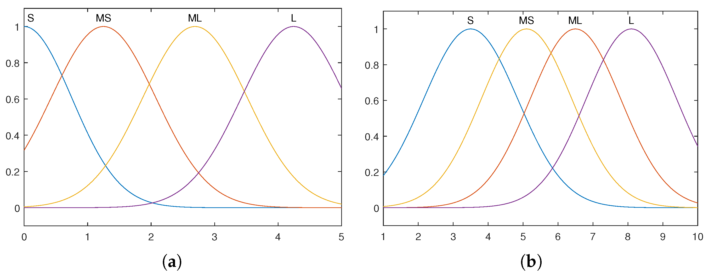
Figure 1. Membership functions of the FLS (S, MS, ML, and L represent small, medium-small, medium-large, and large, respectively): (a) input membership function; (b) output membership function.
Symmetry 17 01359 g001
Figure 2. Numerical experimental results of the FITDRNN model (12) for solving the discrete time-varying matrix problem. (a) The state trajectories of the theoretical solution and the state solution with sampling gap ε = 0.001 . χ 11 denotes the element in the first row and first column of the solution, and the other elements follow the same logic. The red and blue dashed lines represent the theoretical solution and the state solution, respectively. (b) The residual errors of the FITDRNN model (12) with different values of ε .
Symmetry 17 01359 g002
Figure 3. Comparison of the residual errors among the TDRNN model (3), the ADD-RNN model (4), and the FITDRNN model (12) under different sampling gap ε values: (a) ε = 0.01 ; (b) ε = 0.001 ; (c) ε = 0.0001 .
Symmetry 17 01359 g003
Figure 4. Comparison of the residual errors among the TDRNN model (3), the ADD-RNN model (4), and the FITDRNN model (12) in different noise environments with sampling gap ε = 0.001 : (a) constant noise; (b) linear noise; (c) random bounded noise.
Symmetry 17 01359 g004
Figure 5. The results using the FITDRNN model (12) to track the flower-shaped path and performance comparison of different models under noise-free conditions. (a) Motion trajectories of the robotic arm. (b) Actual trajectory and desired path of the robot end-effector. (c) Error between the actual trajectories and the desired trajectories of the X, Y, and Z axes. (d) Comparison of the residual errors among the TDRNN model (3), the ADD-RNN model (4), and the FITDRNN model (12).
Symmetry 17 01359 g005
Figure 6. Comparison of the residual errors of the TDRNN model (3), the ADD-RNN model (4), and the FITDRNN model (12) under different noise conditions in the mechanical arm application: (a) constant noise; (b) linear noise; (c) random bounded noise.
Symmetry 17 01359 g006
Table 1. Comparison of the residual errors among the TDRNN model (3), the ADD-RNN model (4), and the FITDRNN model (12) under different types of noise in the numerical experiment.
CNLNRBN
TDRNN model 3.3333 × 10 1 3.3333 × 10 1 3.3333 × 10 1
ADD-RNN model 1.6666 × 10 1 1.7996 × 10 1 9.8022 × 10 2
FITDRNN model 3.4785 × 10 7 4.9711 × 10 4 3.8973 × 10 3
CN, LN, and RBN denote constant noise U ( t h ) = 50 , linear noise U ( t h ) = 50 + t h , and random bounded noise U ( t h ) [ 55 , 60 ] , respectively.
Table 2. Comparison of the residual errors of the FITDRNN model (12) under different sampling gaps ε and noise types in the numerical experiment.
ε CNLNRBN
0.01 3.5045 × 10 5 4.9834 × 10 3 3.7254 × 10 2
0.001 3.4785 × 10 7 4.9716 × 10 4 2.0401 × 10 3
0.0001 3.4759 × 10 9 4.9696 × 10 5 1.7242 × 10 4
CN, LN, and RBN denote constant noise U ( t h ) = 50 , linear noise U ( t h ) = 50 + t h , and random bounded noise U ( t h ) [ 55 , 60 ] , respectively.
Disclaimer/Publisher’s Note: The statements, opinions and data contained in all publications are solely those of the individual author(s) and contributor(s) and not of MDPI and/or the editor(s). MDPI and/or the editor(s) disclaim responsibility for any injury to people or property resulting from any ideas, methods, instructions or products referred to in the content.