The Inverted Hjorth Distribution and Its Applications in Environmental and Pharmaceutical Sciences

Abstract

This study introduces an inverted version of the three-parameter Hjorth lifespan model, characterized by one scale parameter and two shape parameters, referred to as the inverted Hjorth (IH) distribution. This asymmetric distribution can fit various positively skewed datasets more accurately than several existing models in the literature, as it can accommodate data exhibiting an inverted (upside-down) bathtub-shaped hazard rate. We derive key properties of the model, including quantiles, moments, reliability measures, stress–strength reliability, and order statistics. Point estimation of the IH model parameters is performed using maximum likelihood and Bayesian approaches. Moreover, for interval estimation, two types of asymptotic confidence intervals and two types of Bayesian credible intervals are obtained using the same estimation methodologies. As an extension to a complete sampling plan, Type-II censoring is employed to examine the impact of data incompleteness on IH parameter estimation. Monte Carlo simulation results indicate that Bayesian point and credible estimates outperform those obtained via classical estimation methods across several precision metrics, including mean squared error, average absolute bias, average interval length, and coverage probability. To further assess its performance, two real datasets are analyzed: one from the environmental domain (minimum monthly water flows of the Piracicaba River) and another from the pharmacological domain (plasma indomethacin concentrations). The superiority and flexibility of the inverted Hjorth model are evaluated and compared with several competing models. The results confirm that the IH distribution provides a better fit than several existing lifetime models—such as the inverted Gompertz, inverted log-logistic, inverted Lomax, and inverted Nadarajah–Haghighi distributions—making it a valuable tool for reliability and survival data analysis.

1. Introduction

The Hjorth distribution, proposed by Hjorth [1], is known for accommodating increasing, decreasing, and bathtub-shaped hazard rates, making it more flexible than traditional models such as the Weibull and Gamma distributions. This flexibility enables improved statistical fitting in survival analysis, reliability engineering, and risk assessment.

Furthermore, Hjorth [1] demonstrated that a bathtub-shaped model allows for more effective analysis of failure data from hydromechanical systems driving electric generators in airplanes operating at constant revolutions per unit time. Consequently, this model is widely applied in biostatistics, actuarial science, and mechanical failure analysis, offering improved predictive accuracy for real-world failure data. Following Haj Ahmad and Elshahhat [2], let Y be a nonnegative random variable that follows the three-parameter Hjorth ($\Omega$) distribution, where $\Omega ={(\alpha ,\beta ,\theta )}^{\top }$. 

Then, the associated cumulative distribution function (CDF) and probability density function (PDF) (for $y>0$) of the IH model are given, respectively, by 

$$G\left(y;\Omega \right)=1-{\left(1+\theta y\right)}^{-{\displaystyle \frac{\alpha }{\theta }}}{e}^{-\beta {\displaystyle \frac{y^2}{2}}},y>0,$$

(1)

and

$$g\left(y;\Omega \right)=(\alpha +\beta y\left(1+\theta y\right)){\left(1+\theta y\right)}^{-{\displaystyle \frac{\alpha }{\theta }}-1}{e}^{-\beta {\displaystyle \frac{y^2}{2}}},y>0,$$

(2)

where $(\alpha ,\theta )$ and $\beta$ are the positive shape and scale parameters, respectively. Several authors in the literature have studied this model in different statistical scenarios; for example, see Nadarajah [3], Rastogi et al. [4], Jiang [5], Pushkarna et al. [6], Elshahhat and Nassar [7], Demirci Bicer [8], among others.

An inverted distribution is developed by applying a reciprocal transformation to a random variable. This type of distribution offers enhanced modeling flexibility by introducing distinct hazard rate shapes, such as inverted-bathtub forms, which are suitable for systems with early high risk followed by stabilization. They often provide better fits for real-world data, especially in sciences where large survival times or low failure rates are common; see Lehmann and Shaffer [9], Sharma et al. [10], Nguyen et al. [11], Tomer and Panwar [12], Choudhary et al. [13], Nayal [14], Alqasem et al. [15], Singh et al. [16], among others.

The Hjorth distribution is well-known for its ability to model bathtub-shaped hazard rates, which are important in many reliability settings. However, in real-world applications, especially in biomedical and environmental contexts, data often exhibit inverted bathtub-shaped hazard rates, characterized by early failure risk, a stable middle period, and a declining risk later on. Such behavior is not captured adequately by the original Hjorth model.

The proposed inverted Hjorth (IH) model originates from a non-trivial transformation of the classical Hjorth distribution, capturing inverse behavior in lifetime dynamics, which is rarely addressed in conventional reliability models. The IH model supports an inverted bathtub-shaped hazard rate, which is critical for systems prone to initial high risk, followed by a plateau, and then gradual wear-out—an area underrepresented in traditional survival analysis. The IH model introduces additional flexibility in modeling right-skewed, heavy-tailed data and offers superior capability for capturing extreme values or outliers, especially in biomedical and environmental reliability contexts. Additionally, its hazard function supports more complex reliability structures, which are not well captured by other inverted lifetime models, such as the inverted Weibull or inverted Gompertz lifespan models. Analyzing two real-world datasets from different sectors, as shown later, revealed that the IH distribution outperforms eight existing and recently proposed models, namely inverted Dagum, generalized inverse Gompertz, inverted log-logistic, inverted Lomax, inverted Gompertz, inverted Nadarajah-Haghighi, inverted exponentiated Pareto, and exponentiated inverted exponential. In light of the primary purpose of introducing the IH distribution, the main objectives of the present study are as follows:

• Developing an inverted life distribution, called the IH distribution, which provides a useful framework for modeling data showing inverted bathtub failure rates, demonstrating its superior performance compared to many existing distributions developed in the literature.
• Developing different statistical and reliability characteristics of the IH model, including quantiles, moments, reliability measures, and order statistics.
• Developing different estimators using likelihood- and Bayesian-based approaches to examine the behavior of IH model parameters in estimation scenarios, particularly using Type-II censoring (TIIC).
• Creating two types of asymptotic interval estimators and two types of credible interval estimators.
• Conducting a simulation study to evaluate the accuracy of various estimation methods using rigorous statistical performance metrics.
• Analyzing two real-world datasets to demonstrate the IH distribution’s superiority over existing lifespan distributions in modeling environmental and pharmacological problems, owing to the flexibility and simplicity of its PDF and CDF.

We now classify the rest of this work as follows: Section 2 introduces the IH distribution. Section 3 derives certain model features. Section 4 investigated several parameter estimation issues. Simulation design and real-world data applications are examined in Section 5 and Section 6, respectively. Section 7 and Section 8 outline the study limitations and conclusions, respectively.

2. The Inverted Hjorth Model

This section introduces the key mathematical properties of the IH distribution, including its main functions such as probability density, cumulative distribution, reliability, failure rate, and others.

2.1. Distribution Functions

Now, let Y be a random variable that follows the Hjorth distribution with the CDF $G(·)$, in (1), and with the PDF $g(·)$, in (2). Taking $X=Y^{-1}$, the random variable X will follow the IH model, symbolized as $X\sim \mathrm{IH}(\Omega )$, with the following CDF (say, $F(·)$) and PDF (say, $f(·)$):

$$F\left(x;\Omega \right)={\left(1+{\displaystyle \frac{\theta }{x}}\right)}^{-{\displaystyle \frac{\alpha }{\theta }}}{e}^{-{\displaystyle \frac{\beta }{2x^2}}},x>0,$$

(3)

and

$$f\left(x;\Omega \right)={\displaystyle \frac{1}{x^2}}\left(\alpha +{\displaystyle \frac{\beta }{x}}\left(1+{\displaystyle \frac{\theta }{x}}\right)\right){\left(1+{\displaystyle \frac{\theta }{x}}\right)}^{-{\displaystyle \frac{\alpha }{\theta }}-1}{e}^{-{\displaystyle \frac{\beta }{2x^2}}},$$

(4)

respectively, where $(\alpha ,\theta )$ denotes the shape parameters and $\beta$ denotes the scale parameter. Briefly, to ensure the mathematical validity of the proposed distribution, we now demonstrate that the CDF in (3) satisfies the fundamental properties required of any distribution function.

Proof. 

Specifically, we show the CDF (3) is right-continuous and non-decreasing and that its limiting values at the boundaries of its support conform to standard behavior; that is, the CDF approaches 0 as $x\to 0^{+}$ and approaches 1 as $x\to \infty$.

(i)

Right-Continuity: The function $F(·)$ is composed of rational and exponential components, each continuous for $x>0$. Hence, the function is right-continuous, such as:

$$\underset{h\to 0^{+}}{lim}F(x+h;\Omega )=F(x;\Omega ).$$

(ii)

Limits at the Endpoints:

• As $x\to 0^{+}$, we get: ${\left(1+{\displaystyle \frac{\theta }{x}}\right)}^{-{\displaystyle \frac{\alpha }{\theta }}}\to 0,exp\left(-{\displaystyle \frac{\beta }{2x^2}}\right)\to 0\Rightarrow \underset{x\to 0^{+}}{lim}F(x;\Omega )=0.$
• As $x\to \infty$, we get: ${\left(1+{\displaystyle \frac{\theta }{x}}\right)}^{-{\displaystyle \frac{\alpha }{\theta }}}\to 1,exp\left(-{\displaystyle \frac{\beta }{2x^2}}\right)\to 1\Rightarrow \underset{x\to \infty }{lim}F(x;\Omega )=1.$

(iii)

Monotonicity (Non-decreasing): Check the PDF by differentiating the CDF with respect to x:

$$\begin{array}{cc}\hfill f(x;\Omega )& ={\displaystyle \frac{d}{dx}}F(x;\Omega )\hfill \\ \hfill & ={\left(1+{\displaystyle \frac{\theta }{x}}\right)}^{-{\displaystyle \frac{\alpha }{\theta }}}exp\left(-{\displaystyle \frac{\beta }{2x^2}}\right)\left({\displaystyle \frac{\alpha }{x^2+\theta x}}+{\displaystyle \frac{\beta }{x^3}}\right),\hfill \end{array}$$

which is matches to Equation (4), that is

$$f(x;\Omega )={\displaystyle \frac{1}{x^2}}\left(\alpha +{\displaystyle \frac{\beta }{x}}\left(1+{\displaystyle \frac{\theta }{x}}\right)\right){\left(1+{\displaystyle \frac{\theta }{x}}\right)}^{-{\displaystyle \frac{\alpha }{\theta }}-1}{e}^{-{\displaystyle \frac{\beta }{2x^2}}}.$$

(5)

Since all terms in (5) are strictly positive for $x>0$ and $\alpha ,\beta ,\theta >0$, it follows that $f(·)>0$, and thus $F(·)$ is strictly increasing (non-decreasing) on its support.

   □

2.2. Reliability and Failure Rate

The survival (or reliability) and hazard rate (or failure rate function (FRF)) functions of the IH distribution are

$$R\left(x;\Omega \right)=1-{\left(1+{\displaystyle \frac{\theta }{x}}\right)}^{-{\displaystyle \frac{\alpha }{\theta }}}{e}^{-{\displaystyle \frac{\beta }{2x^2}}},$$

(6)

and

$$h\left(x;\Omega \right)={\displaystyle \frac{\frac{1}{x^2}\left(\alpha +\frac{\beta }{x}\left(1+\frac{\theta }{x}\right)\right){\left(1+\frac{\theta }{x}\right)}^{-\frac{\alpha }{\theta }-1}{e}^{-\frac{\beta }{2x^2}}}{1-{\left(1+\frac{\theta }{x}\right)}^{-\frac{\alpha }{\theta }}{e}^{-\frac{\beta }{2x^2}}}}.$$

(7)

By varying the parameters $\alpha$, $\theta$, and $\beta$, Figure 1 illustrates different shapes of the density and hazard rate functions of the IH model. Figure 1a shows that the IH density can be unimodal and positively (right) skewed, exhibiting substantial tail heaviness. Figure 1b illustrates that the IH hazard rate exhibits an inverted (upside-down) bathtub shape. This type of failure rate is relevant for modeling early-life failures, stable operational phases, and wear-out failures, making it highly suitable for real-world reliability analysis. It is useful for optimizing maintenance schedules, designing cost-effective warranty policies, and improving resource allocation by emphasizing early defect detection and late-stage preventive actions. Consequently, Figure 1 shows that:

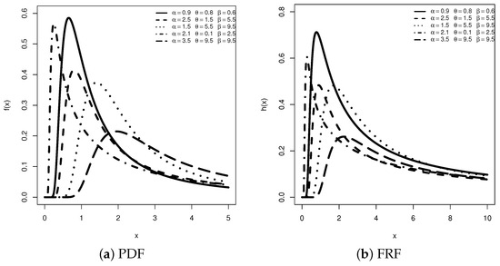
Figure 1. Several density and failure rate shapes of the IH’s model.

• When $\alpha$ is small and $\beta$ is moderate, the PDF exhibits pronounced right skewness and heavy tails;
• When $\theta$ is small, the FRF assumes a monotonically decreasing shape;
• As $\theta$ increases, the FRF adopts an inverted bathtub shape, rising initially, peaking early, and then gradually declining;
• Increasing $\beta$ compresses the PDF toward the origin, producing a sharper peak and accentuating the early-failure phase in the FRF.

2.3. Density Expansion

The series expansion of the IH density provides deeper insight into the distribution’s structure, particularly when analyzing its behavior near the origin or in the tails. Although the PDF (4) is expressed in closed form and is algebraically tractable, representing it via a Maclaurin series expansion enhances its analytical utility. Accordingly, this part derives a power series representation of the IH density to facilitate further theoretical exploration. Suppose $a>0$ and $b>0$ are real numbers; we now employ the following general binomial expansion series:

$${\left(1+a\right)}^b=\sum _{i=0}^{\infty }\left(\begin{array}{c}b\\ i\end{array}\right)a^i,$$

(8)

where $\left(\begin{array}{c}b\\ i\end{array}\right)={\displaystyle \frac{\Gamma (b+1)\Gamma (i+1)}{\Gamma (b-i+1)}}$.

Applying the expansion (8) to the case where the numerator coefficient is negative, we obtain:

$${\left(1+{\displaystyle \frac{\theta }{x}}\right)}^{-{\displaystyle \frac{\alpha }{\theta }}-1}=\sum _{i=0}^{\infty }{\left(-1\right)}^i\left(\begin{array}{c}\alpha {\theta }^{-1}+i\\ i\end{array}\right){\left({\displaystyle \frac{\theta }{x}}\right)}^i,$$

(9)

expanding the PDF (4) by (9), we get

$$f\left(x\right)=\sum _{i=0}^{\infty }{\psi }_i^{\circ }{\theta }^i{\displaystyle \frac{1}{x^{i+2}}}\left(\alpha +{\displaystyle \frac{\beta }{x}}\left(1+{\displaystyle \frac{\theta }{x}}\right)\right)e^{-{\displaystyle \frac{\beta }{2x^2}}},x>0,\alpha ,\theta ,\beta >0,$$

(10)

where ${\psi }_i^{\circ }={\left(-1\right)}^i{\displaystyle \frac{\Gamma \left(\alpha {\theta }^{-1}+i+1\right)}{\Gamma \left(i+1\right)\Gamma \left(\alpha {\theta }^{-1}+1\right)}}$.

Setting $\left(\alpha +{\displaystyle \frac{\beta }{x}}\left(1+{\displaystyle \frac{\theta }{x}}\right)\right)={\displaystyle \sum _{j=0}^2}{\displaystyle \frac{A_j}{x^j}}$ and $e^{-{\displaystyle \frac{\beta }{2x^2}}}={\displaystyle \sum _{k=0}^{\infty }}{\displaystyle \frac{{\left(-1\right)}^k}{\Gamma \left(k+1\right)}}{\left({\displaystyle \frac{\beta }{2x^2}}\right)}^k$, one can rewrite (10) as:

$$f\left(x\right)=\sum _{i,k=0}^{\infty }\sum _{j=0}^2{\psi }_{i,k}^{\circ }{A}_j{\theta }^i{\beta }^k{\displaystyle \frac{2^{-k}}{x^{i^{*}}}},x>0,\alpha ,\theta ,\beta >0,$$

(11)

where $i^{*}=i+j+2(k+1)$, $A_0=\alpha$, $A_1=\beta$, $A_2=\beta \theta$, and ${\psi }_{i,k}^{\circ }={\displaystyle \frac{{\left(-1\right)}^k}{\Gamma \left(k+1\right)}}{\psi }_i^{\circ }$.

In similar setup, from (9), we expanding the following term:

$${\left(1+{\displaystyle \frac{\theta }{x}}\right)}^{-{\displaystyle \frac{\alpha }{\theta }}}=\sum _{i=0}^{\infty }{\left(-1\right)}^i\left(\begin{array}{c}\alpha {\theta }^{-1}+i-1\\ i\end{array}\right){\left({\displaystyle \frac{\theta }{x}}\right)}^i,$$

(12)

thus, we can easily expanding the CDF (3) as follows:

$$F\left(x\right)=\sum _{i,k=0}^{\infty }{\psi }_{i,k}^{•}{\displaystyle \frac{{\theta }^i{\beta }^k}{x^{2k+i}}},x>0,$$

(13)

where ${\psi }_{i,k}^{•}={\left(-1\right)}^{i+k}{\displaystyle \frac{\Gamma \left(\alpha {\theta }^{-1}+i\right)}{2^k\Gamma \left(i+1\right)\Gamma \left(\alpha {\theta }^{-1}\right)\Gamma \left(k+1\right)}}.$

Notably, the infinite series expansions of the PDF and CDF given in (11) and (13), respectively, are numerically approximated by truncating both series to a finite number of terms, denoted $i_{max}$ and $k_{max}$. From a simulated IH dataset, without loss of generality, truncating at $i_{max}=10$ and $k_{max}=10$ yields an accurate approximation with a negligible error (less than 10⁻⁶) across the entire range of practical parameter values.

2.4. Quantile and Quartiles

The quantile function, given by $Q\left(u\right)=F^{-1}\left(u\right)$ for $0<u<1$, can be derived from (3) as

$$Q\left(u\right)=F^{-1}\left(u\right),0<u<1,$$

(14)

solve for x in terms of u, we get:

$$u={\left(1+{\displaystyle \frac{\theta }{x}}\right)}^{-{\displaystyle \frac{\alpha }{\theta }}}{e}^{-{\displaystyle \frac{\beta }{2x^2}}}.$$

Taking the natural logarithm for both sides as

$$log\left(1+{\displaystyle \frac{\theta }{x}}\right)=-{\displaystyle \frac{\theta }{\alpha }}\left[log\left(u\right)+{\displaystyle \frac{\beta }{2x^2}}\right].$$

(15)

After raising both sides in (15) to the power, we put $e^{-{\displaystyle \frac{\theta }{\alpha }}log\left(u\right)}=u^{-{\displaystyle \frac{\theta }{\alpha }}}$ as follows

$$x\left(u\right)={\displaystyle \frac{\theta }{u^{-\frac{\theta }{\alpha }}{e}^{-\frac{\theta \beta }{2\alpha x^2}}-1}}.$$

(16)

As a result, the quantile function of the IH model is expressed in a nonlinear form and requires numerical methods to solve for x. Now, let U follow the uniform distribution on (0, 1). Then, a random sample of size n from the IH distribution can be generated as follows:

$$x_i={\displaystyle \frac{\theta }{u_i^{-\frac{\theta }{\alpha }}{e}^{-\frac{\theta \beta }{2\alpha x_i^2}}-1}},i=1,\dots ,n.$$

For this purpose, we recommend using the ’$\mathsf{GoFKernel}$’ package (version 2.1-3), as suggested by Pavia and Pavia [17], to simulate IH random variates. In particular, from (16), the first, second (median), and third quartiles of the IH distribution can be acquired directly by setting $u(={\displaystyle \frac{1}{4}},{\displaystyle \frac{2}{4}},{\displaystyle \frac{3}{4}})$, respectively.

3. Statistical Properties

This section presents several properties of the IH distribution, including moments, mean residual life, stress–strength reliability, and order statistics, among others.

3.1. Mean Deviation

The mean deviation about the mean (or median) offers a simple and intuitive measure of dispersion, as it captures the average absolute deviation of data points from the central value, making it useful for understanding variability within a population. Let $\mu$ and M denote the mean and median of the IH distribution, respectively. Following Elshahhat et al. [18], the mean deviation about the mean $\mu$ (say, ${\mathcal{D}}_{\mu }\left(X\right)$) can be derived as

$$\begin{array}{cc}\hfill {\mathcal{D}}_{\mu }\left(X\right)=\mathbb{E}\left(\left|X-\mu \right|\right)& ={\int }_{-\infty }^{\infty }\left|x-\mu \right|f\left(x\right)dx\hfill \\ \hfill & =2[\mu F\left(\mu \right)-\phi \left(\mu \right)],\hfill \end{array}$$

(17)

where $\phi \left(\mu \right)={\int }_0^{\mu }xf\left(x\right)dx.$ From (11), one can get $\phi \left(\mu \right)$ as

$$\begin{array}{cc}\hfill \phi \left(\mu \right)& =\sum _{i,k=0}^{\infty }\sum _{j=0}^2{\psi }_{i,k}^{\circ }{A}_j{\theta }^i{\beta }^k{\int }_0^t{\displaystyle \frac{2^{-k}}{x^{i^{*}-1}}}dx,\hfill \\ \hfill & =\sum _{i,k=0}^{\infty }\sum _{j=0}^2{\psi }_{i,k}^{\circ }{A}_j{\theta }^i{\beta }^k{2}^{-k}{\displaystyle \frac{{\mu }^{1-i^{*}}}{(1-i^{*})}}.\hfill \end{array}$$

(18)

Now, from (3) and (18), one can re-express (17) as

$$\begin{array}{c}\hfill {\mathcal{D}}_{\mu }\left(X\right)=2\left[\mu F\left(\mu \right)-\sum _{i,k=0}^{\infty }\sum _{j=0}^2{\psi }_{i,k}^{\circ }{A}_j{\theta }^i{\beta }^k{2}^{-k}{\displaystyle \frac{{\mu }^{1-i^{*}}}{(1-i^{*})}}\right].\end{array}$$

(19)

On the other hand, the mean deviation about the median M of the IH distribution is given by

$$\begin{array}{cc}\hfill {\mathcal{D}}_2\left(X\right)=\mathbb{E}\left(\left|X-M\right|\right)& ={\int }_{-\infty }^{\infty }\left|x-M\right|f\left(x\right)dx\hfill \\ \hfill & =\mu -2\phi \left(M\right).\hfill \end{array}$$

(20)

By replacing $\mu$ with M in (18), the mean deviation about the median, denoted ${\mathcal{D}}_2\left(X\right)$, can be derived in a manner similar to that used for obtaining the mean deviation about the mean $\mu$ of the IH distribution.

3.2. Moments and Moment Generating Function

Moments play a vital role in statistical analysis, as they characterize important features of probability distributions

Theorem 1.

If X follows the IH$(\Omega )$ distribution, then the rth moment (moment about zero), denoted ${\mu }_r^{\circ }$, is given by

$$\begin{array}{c}\hfill {\mu }_r^{\circ }={\displaystyle \frac{1}{2}}\sum _{v=0}^{\infty }{(-1)}^v{\displaystyle \frac{\Gamma (\nu +v)}{\Gamma \left(\nu \right)\Gamma (v+1)}}{\theta }^v\left(\alpha {\mathcal{K}}_{1,r,v}^{★}+\beta {\mathcal{K}}_{2,r,v}^{★}+\beta \theta {\mathcal{K}}_{3,r,v}^{★}\right),\end{array}$$

(21)

where

• ${\mathcal{K}}_{1,r,v}^{★}={\left({\displaystyle \frac{\beta }{2}}\right)}^{-{\displaystyle \frac{(3-r+v)}{2}}}\Gamma \left({\displaystyle \frac{3-r+v}{2}}\right),$
• ${\mathcal{K}}_{2,r,v}^{★}={\left({\displaystyle \frac{\beta }{2}}\right)}^{-{\displaystyle \frac{(4-r+v)}{2}}}\Gamma \left({\displaystyle \frac{4-r+v}{2}}\right),$

and

• ${\mathcal{K}}_{3,r,v}^{★}={\left({\displaystyle \frac{\beta }{2}}\right)}^{-{\displaystyle \frac{(5-r+v)}{2}}}\Gamma \left({\displaystyle \frac{5-r+v}{2}}\right).$

Proof. 

See Appendix A.    □

By setting $r=1$ in (21), the mean of the IH distribution is

$${\mu }_1^{\circ }={\displaystyle \frac{1}{2}}\sum _{v=0}^{\infty }{(-1)}^v{\displaystyle \frac{\Gamma (\nu +v)}{\Gamma \left(\nu \right)\Gamma (v+1)}}{\theta }^v\left(\alpha {\mathcal{K}}_{1,1,v}^{★}+\beta {\mathcal{K}}_{2,1,v}^{★}+\beta \theta {\mathcal{K}}_{3,1,v}^{★}\right),$$

(22)

where

• ${\mathcal{K}}_{1,1,v}^{★}={\left({\displaystyle \frac{\beta }{2}}\right)}^{-{\displaystyle \frac{(2+v)}{2}}}\Gamma \left({\displaystyle \frac{2+v}{2}}\right),$
• ${\mathcal{K}}_{2,1,v}^{★}={\left({\displaystyle \frac{\beta }{2}}\right)}^{-{\displaystyle \frac{(3+v)}{2}}}\Gamma \left({\displaystyle \frac{3+v}{2}}\right),$

and

• ${\mathcal{K}}_{3,1,v}^{★}={\left({\displaystyle \frac{\beta }{2}}\right)}^{-{\displaystyle \frac{(4+v)}{2}}}\Gamma \left({\displaystyle \frac{4+v}{2}}\right).$

Following the same approach used to obtain the mean of the IH model, its variance can be derived as $V\left(X\right)={\mu }_2={\mu }_2^{\circ }-{\left({\mu }_1^{\circ }\right)}^2$, by directly setting $r=2$ in ${\mu }_r^{\circ }$.

Using Theorem 1, the central moments of the IH distribution can be obtained in the following form:

$${\mu }_r^{•}=\sum _{j=0}^r{(-1)}^j\left(\begin{array}{c}r\\ j\end{array}\right){\mu }_1^{\circ }{\mu }_{r-j}^{\circ }.$$

(23)

Using ${\mu }_i^{•}$ for $i=2,3,4$, the skewness, denoted by ${\Psi }_1$, and the kurtosis, denoted by ${\Psi }_2$, of the IH distribution can be obtained, respectively, as follows:

$${\Psi }_1={\displaystyle \frac{{\mu }_3^{•}}{{\left({\mu }_2^{•}\right)}^{\frac{3}{2}}}}\mathrm{and}{\Psi }_2={\displaystyle \frac{{\mu }_4^{•}}{{\left({\mu }_2^{•}\right)}^2}}.$$

Table 1 presents key summary statistics of the IH distribution, namely the mean, variance, skewness, and kurtosis. The results indicate that:

Table 1. Summary statistics of the IH model under different parameter settings.

$\mathit{\alpha }$	$\mathit{\beta }\to$	0.5				1.0				1.5
	$\mathbf{\theta }\downarrow$	Mean	Variance	Skewness	Kurtosis	Mean	Variance	Skewness	Kurtosis	Mean	Variance	Skewness	Kurtosis
0.5	0.1	0.302	0.101	0.509	1.703	0.264	0.106	0.761	1.856	0.219	0.123	1.082	2.380
	0.5	0.312	0.104	0.443	1.707	0.278	0.111	0.668	1.746	0.233	0.126	0.983	2.184
	1.0	0.323	0.107	0.377	1.711	0.291	0.117	0.585	1.661	0.245	0.128	0.898	2.032
	1.5	0.332	0.111	0.327	1.717	0.302	0.121	0.526	1.607	0.254	0.130	0.838	1.931
	2.5	0.345	0.116	0.255	1.734	0.316	0.126	0.443	1.544	0.267	0.132	0.756	1.806
1.0	0.1	0.204	0.102	1.160	2.670	0.172	0.100	1.454	3.362	0.141	0.093	1.799	4.452
	0.5	0.224	0.105	1.002	2.385	0.193	0.102	1.262	2.862	0.159	0.100	1.590	3.751
	1.0	0.242	0.107	0.864	2.177	0.213	0.103	1.100	2.495	0.177	0.107	1.418	3.235
	1.5	0.257	0.109	0.763	2.048	0.228	0.106	0.985	2.265	0.190	0.111	1.297	2.909
	2.5	0.278	0.112	0.623	1.906	0.251	0.109	0.828	1.995	0.210	0.118	1.136	2.519
1.5	0.1	0.134	0.085	1.844	4.713	0.111	0.076	2.191	6.070	0.090	0.065	2.590	7.963
	0.5	0.157	0.091	1.570	3.822	0.133	0.085	1.872	4.786	0.108	0.075	2.236	6.252
	1.0	0.180	0.095	1.347	3.207	0.154	0.093	1.614	3.896	0.127	0.085	1.955	5.071
	1.5	0.197	0.098	1.190	2.837	0.172	0.095	1.437	3.359	0.142	0.091	1.764	4.357
	2.5	0.224	0.105	0.978	2.416	0.198	0.102	1.200	2.743	0.166	0.099	1.515	3.533

• When $\alpha$ increases (for fixed $\theta$ and $\beta$), the mean and variance decrease, whereas the skewness and kurtosis increase. A similar pattern is observed when $\beta$ increases (for fixed $\alpha$ and $\theta$);
• When $\theta$ increases (for fixed $\alpha$ and $\beta$), the mean and variance increase, while the skewness and kurtosis decrease.

The moment generating function (say, ${\mathcal{M}}_X(·)$) is defined as

$$\begin{array}{cc}\hfill {\mathcal{M}}_X\left(t\right)& =\sum _{r=0}^{\infty }{\displaystyle \frac{t^r}{\Gamma (r+1)}}{\int }_0^{\infty }{x}^{r}f\left(x\right)dx,\hfill \\ \hfill & =\sum _{r=0}^{\infty }{\displaystyle \frac{t^r}{\Gamma (r+1)}}{\mu }_r^{\circ }.\hfill \end{array}$$

(24)

Then, from (4) and (21), we have

$${\mathcal{M}}_X\left(t\right)={\displaystyle \frac{1}{2}}\sum _{v,r=0}^{\infty }{B}_{v,r}^{\circ }{\theta }^v\left(\alpha {\mathcal{K}}_{1,r,v}^{★}+\beta {\mathcal{K}}_{2,r,v}^{★}+\beta \theta {\mathcal{K}}_{3,r,v}^{★}\right),$$

where

$$B_{v,r}^{\circ }={(-1)}^v{\displaystyle \frac{t^r\Gamma (\nu +v)}{\Gamma \left(\nu \right)\Gamma (v+1)\Gamma (r+1)}}.$$

3.3. Mean Residual Life

The mean residual life (MRL) function quantifies the expected remaining lifetime of a system or component, given that it has survived up to a specified time. This measure is particularly useful in reliability analysis and maintenance planning. The MRL function, denoted by $\mathrm{MRL}(·)$, is defined as

$$\begin{array}{cc}\hfill \mathrm{MRL}\left(t\right)& ={\displaystyle \frac{1}{R\left(t\right)}}{\int }_t^{\infty }R\left(x\right)dx\hfill \\ \hfill & ={\displaystyle \frac{1}{R\left(t\right)}}\left({\int }_t^{\infty }xf\left(x\right)dx-t\right)\hfill \\ \hfill & ={\displaystyle \frac{1}{R\left(t\right)}}\left({\mu }_1^{\circ }-t-{\int }_0^{t}xf\left(x\right)dx\right),t>0,\hfill \end{array}$$

(25)

where $R\left(t\right)$ and ${\mu }_1^{\circ }$ are defined in (6) and (22), respectively.

Substituting (11) into (25), the MRL function of the IH model, for $t>0$, is obtained as:

$$\begin{array}{cc}\hfill \mathrm{MRL}\left(t\right)& ={\displaystyle \frac{1}{R\left(t\right)}}\left({\mu }_1^{\circ }-t-\sum _{i,k=0}^{\infty }\sum _{j=0}^2{\psi }_{i,k}^{\circ }{A}_j{\theta }^i{\beta }^k{\int }_0^t{\displaystyle \frac{2^{-k}}{x^{i^{*}-1}}}dx\right),\hfill \\ \hfill & ={\displaystyle \frac{1}{R\left(t\right)}}\left({\mu }_1^{\circ }-t-\sum _{i,k=0}^{\infty }\sum _{j=0}^2{\psi }_{i,k}^{\circ }{A}_j{\theta }^i{\beta }^k{2}^{-k}{\displaystyle \frac{t^{2-i^{*}}}{(2-i^{*})}}\right),t>0.\hfill \end{array}$$

(26)

3.4. Mean Inactivity Time

The mean inactivity time (MIT) function quantifies the expected time a system or component has been inactive prior to a given time and is useful in reliability and maintenance analysis. Consider the quantity $\left(x-X\right)|X\le x$, where X is a lifetime random variable. This represents the elapsed time since the component failed, given that its lifetime is less than or equal to x. The MIT function of X is formally defined as

$$\begin{array}{cc}\hfill \mathrm{MIT}\left(t\right)& =\mathbb{E}(t-X|X\le t)={\displaystyle \frac{{\int }_0^{t}F\left(x\right)dx}{F\left(t\right)}}.\hfill \end{array}$$

(27)

If $X\sim \mathrm{IH}(\Omega )$, from (13), we have

$${\int }_0^{t}F\left(x\right)dx=\sum _{i,k=0}^{\infty }{\psi }_{i,k}^{•}{\theta }^i{\beta }^k{\displaystyle \frac{t^{1-i-2k}}{(1-i-2k)}},t>0.$$

(28)

By substituting (13) and (28) into (27), the MIT function (for $t>0$) of the IH distribution can be obtained.

3.5. Strong Mean Inactivity Time

The strong-MIT (SMIT) function is used in reliability analysis, maintenance scheduling, and risk assessment to evaluate system downtime, predict failure patterns, and optimize resource allocation for improved operational efficiency.

The SMIT of a lifetime $rv$ X is defined as

$$\mathrm{SMIT}\left(t\right)={\displaystyle \frac{1}{F\left(t\right)}}{\int }_0^{t}2xF\left(x\right)dx.$$

(29)

If $X\sim \mathrm{IH}(\Omega )$, from (13), we have

$${\int }_0^{t}2xF\left(x\right)dx=\sum _{i,k=0}^{\infty }{\psi }_{i,k}^{•}{\theta }^i{\beta }^k{\displaystyle \frac{t^{2\left(1-k\right)-i}}{2\left(1-k\right)-i}},t>0.$$

(30)

Subsequently, the SMIT of the IH distribution can be simply offered by substituting (13) (at $t>0$) and (30) into (29).

3.6. Stress-Strength

In the stress–strength model, the lifetime of a component with random strength, denoted $X_1$, under random stress, denoted $X_2$, is considered. The component fails when the applied stress exceeds its strength, i.e., when $X_2>X_1$, and remains functional otherwise. Suppose $X_1$ and $X_2$ are independent IH random variables such that $X_1\sim \mathrm{IH}({\alpha }_1,\beta ,{\theta }_1)\mathrm{and}{X}_2\sim \mathrm{IH}({\alpha }_2,\beta ,{\theta }_2).$ Then, the stress–strength parameter (SSP), denoted $\mathcal{R}=Pr(X_1>X_2),$ is given by

$$\mathcal{R}={\int }_0^{\infty }{f}_1\left(x;{\alpha }_1,\beta ,{\theta }_1\right)F_2\left(x;{\alpha }_2,\beta ,{\theta }_2\right)dx.$$

(31)

From (3) and (4), the CDF and PDF of $X_1$ and $X_2$ can be formulated as follows:

$$F_2\left(x;{\alpha }_2,\beta ,{\theta }_2\right)={\left(1+{\displaystyle \frac{{\theta }_2}{x}}\right)}^{-{\displaystyle \frac{{\alpha }_2}{{\theta }_2}}}{e}^{-{\displaystyle \frac{\beta }{2x^2}}},x>0,$$

(32)

and

$$f_1\left(x;{\alpha }_1,\beta ,{\theta }_1\right)={\displaystyle \frac{1}{x^2}}\left({\alpha }_1+{\displaystyle \frac{\beta }{x}}\left(1+{\displaystyle \frac{{\theta }_1}{x}}\right)\right){\left(1+{\displaystyle \frac{{\theta }_1}{x}}\right)}^{-{\displaystyle \frac{\alpha }{{\theta }_1}}-1}{e}^{-{\displaystyle \frac{\beta }{2x^2}}},x>0,$$

(33)

respectively, where ${\alpha }_i>0$ and ${\theta }_i>0$ (for $i=1,2$) denote the shape parameters and $\beta$ denotes the scale parameter. Before deriving the SSP, we first determine three key quantities from the expansion series, namely:

$$e^{-{\displaystyle \frac{\beta }{x^2}}}=\sum _{k=0}^{\infty }{\displaystyle \frac{{\left(-1\right)}^k}{\Gamma \left(k+1\right)}}{\left({\displaystyle \frac{\beta }{x^2}}\right)}^k,$$

(34)

$${\left(1+{\displaystyle \frac{{\theta }_1}{x}}\right)}^{-{\displaystyle \frac{{\alpha }_1}{{\theta }_1}}-1}=\sum _{i=0}^{\infty }{\left(-1\right)}^i\left(\begin{array}{c}{\alpha }_1{\theta }_1^{-1}+i\hfill \\ i\hfill \end{array}\right){\left({\displaystyle \frac{{\theta }_1}{x}}\right)}^i$$

(35)

and

$${\left(1+{\displaystyle \frac{{\theta }_2}{x}}\right)}^{-{\displaystyle \frac{{\alpha }_2}{{\theta }_2}}}=\sum _{j=0}^{\infty }{\left(-1\right)}^j\left(\begin{array}{c}{\alpha }_2{\theta }_2^{-1}+j-1\hfill \\ j\hfill \end{array}\right){\left({\displaystyle \frac{{\theta }_2}{x}}\right)}^j.$$

(36)

Substituting Equations (32)–(36) into (31), the SSP $\mathcal{R}$ of the IH model becomes

$$\mathcal{R}=\sum _{i,j,k=0}^{\infty }\sum _{l=0}^2{\psi }_{i,j,k}^{•}{A}_l^{•}{x}^{-\left(i+j+l+2k\right)}{\theta }^{i+j}{\beta }^k,$$

(37)

where $A_0^{•}={\alpha }_1$, $A_1^{•}=\beta$, $A_2^{•}=\beta {\theta }_1$, and

$${\psi }_{i,j,k}^{•}={\left(-1\right)}^{i+j+k}{\displaystyle \frac{\Gamma \left({\alpha }_1{\theta }_1^{-1}+i+1\right)\Gamma \left({\alpha }_2{\theta }_2^{-1}+j\right)}{\Gamma \left(i+1\right)\Gamma \left(j+1\right)\Gamma \left(k+1\right)\Gamma \left({\alpha }_1{\theta }_1^{-1}+1\right)\Gamma \left({\alpha }_2{\theta }_2^{-1}\right)}}.$$

3.7. Order Statistics

Order statistics provide valuable insights into the distribution of data, facilitating the estimation of percentiles, extremes, and reliability measures in statistical analysis. Suppose $X_{\left(1\right)}\le X_{\left(2\right)}\le \dots \le X_{\left(n\right)}$ denote the order statistics of a random sample of size n drawn from the IH population. The PDF and CDF of $X_{\left(m\right)}$, for $m=1,2,\dots ,n$ (denoted by $f_{\left(m\right)}\left(x\right)$ and $F_{\left(m\right)}\left(x\right)$, respectively), where $B(·,·)$ is the beta function, are given by

$$\begin{array}{cc}\hfill f_{\left(m\right)}\left(x\right)& =C_m^{-1}f\left(x\right){\left[F\left(x\right)\right]}^{m-1}{\left[1-F\left(x\right)\right]}^{n-m}\hfill \\ \hfill & =C_m^{-1}\sum _{i=1}^{n-m}{\left(-1\right)}^i\left(\begin{array}{c}n-m\\ i\end{array}\right)f\left(x\right){\left[F\left(x\right)\right]}^{m+i-1},\hfill \end{array}$$

(38)

and

$$\begin{array}{cc}\hfill F_{\left(m\right)}\left(x\right)& =\sum _{m=0}^n\left(\begin{array}{c}n\\ m\end{array}\right){\left[F\left(x\right)\right]}^m{\left[1-F\left(x\right)\right]}^{n-m}\hfill \\ \hfill & =\sum _{m=0}^n\sum _{i=0}^{n-m}{\left(-1\right)}^i\left(\begin{array}{c}n\\ m\end{array}\right)\left(\begin{array}{c}n-m\\ i\end{array}\right){\left[F\left(x\right)\right]}^{m+i},\hfill \end{array}$$

(39)

respectively, where $C_m=B\left(m,n-m+1\right)$.

Hence, from (3) and (4), the PDF and CDF of $X_{\left(m\right)},m=1,2,\dots ,n,$ are acquired, respectively, as 

$$\begin{array}{c}\hfill f_{\left(m\right)}\left(x\right)=C_m^{-1}\sum _{i=1}^{n-m}\sum _{j=0}^2{\left(-1\right)}^i{\displaystyle \frac{A_j}{x^{j+2}}}\left(\begin{array}{c}n-m\\ i\end{array}\right){\left(1+{\displaystyle \frac{\theta }{x}}\right)}^{-\left(m+i\right){\displaystyle \frac{\alpha }{\theta }}-1}{e}^{-\left(m+i\right){\displaystyle \frac{\beta }{2x^2}}}\end{array}$$

(40)

and

$$F_{\left(m\right)}\left(x\right)=\sum _{m=0}^n\sum _{i=0}^{n-m}{\left(-1\right)}^i\left(\begin{array}{c}n\\ m\end{array}\right)\left(\begin{array}{c}n-m\\ i\end{array}\right){\left(1+{\displaystyle \frac{\theta }{x}}\right)}^{-\left(m+i\right){\displaystyle \frac{\alpha }{\theta }}}{e}^{-\left(m+i\right){\displaystyle \frac{\beta }{2x^2}}}.$$

(41)

Consequently, the PDFs of the smallest and largest order statistics, $X_{\left(1\right)}$ and $X_{\left(n\right)}$, respectively, are given by

$$\begin{array}{c}\hfill f_{\left(1\right)}\left(x\right)=C_1^{-1}\sum _{i=1}^{n-1}\sum _{j=0}^2{\left(-1\right)}^i\left(\begin{array}{c}n-1\\ i\end{array}\right){\displaystyle \frac{A_j}{x^{j+2}}}{\left(1+{\displaystyle \frac{\theta }{x}}\right)}^{-\left(i+1\right){\displaystyle \frac{\alpha }{\theta }}-1}{e}^{-\left(i+1\right){\displaystyle \frac{\beta }{2x^2}}}\end{array}$$

and

$$\begin{array}{c}\hfill f_{\left(n\right)}\left(x\right)=C_n^{-1}\sum _{j=0}^2{\displaystyle \frac{A_j}{x^{j+2}}}{\left(1+{\displaystyle \frac{\theta }{x}}\right)}^{-{\displaystyle \frac{\alpha n}{\theta }}-1}{e}^{-{\displaystyle \frac{\beta n}{2x^2}}},\end{array}$$

respectively.

4. Parameter Estimation

This section deals with the likelihood and Bayesian estimation approaches under a TIIC strategy for developing point and interval estimates of the IH parameters.

4.1. Likelihood Inference

Suppose $\mathbf{x}=(X_{\left(1\right)},X_{\left(2\right)},\dots ,X_{\left(d\right)})$, where $d<n$ is the specified number of failures, represents a TIIC sample of size d obtained from a life test of n independent units, all placed on test at time zero. The joint likelihood function of $X_{\left(i\right)},i=1,2,\dots ,d$, denoted $L(·)$, is defined as

$$L\left(\mathbf{x}\right|\Omega )=C_d\prod _{i=1}^d\left[f(x_{\left(i\right)};\Omega )\right]{\left[1-F(x_{\left(d\right)};\Omega )\right]}^{n-d},$$

(42)

where $C_d={\displaystyle \frac{n!}{(n-d)!}}$.

From (3), (4), and (42), the likelihood function (LF) and its corresponding log-likelihood (log-LF) can be expressed, up to a proportionality constant, as 

$$L\left(\mathbf{x}\right|\Omega )\propto {\prod }_{i=1}^d{\varrho }_i{\vartheta }_i^{-{\displaystyle \frac{\alpha }{\theta }}-1}{e}^{-\beta {\sum }_{i=1}^d{\displaystyle \frac{1}{2x_i^2}}}{\left[1-{\vartheta }_d^{-{\displaystyle \frac{\alpha }{\theta }}}{e}^{-{\displaystyle \frac{\beta }{2x_d^2}}}\right]}^{n-d}$$

(43)

and

$$\begin{array}{cc}\hfill logL& ={\sum }_{i=1}^{d}log\left({\varrho }_i\right)-\left({\displaystyle \frac{\alpha }{\theta }}+1\right){\sum }_{i=1}^{d}log\left({\vartheta }_i\right)-\beta {\sum }_{i=1}^d{\displaystyle \frac{1}{2x_i^2}}\hfill \\ \hfill & +\left(n-d\right)log\left[1-{\vartheta }_d^{-{\displaystyle \frac{\alpha }{\theta }}}{e}^{-{\displaystyle \frac{\beta }{2x_d^2}}}\right],\hfill \end{array}$$

(44)

respectively, where ${\varrho }_i=\alpha +\beta x_i^{-1}{\vartheta }_i$ and $x_i\equiv x_{\left(i\right)},i=1,2,...,m,$ for simplicity.

By differentiating (44) partially with respect to $\alpha$, $\beta$, and $\theta$, three nonlinear likelihood equations are obtained, which must be solved simultaneously to obtain their maximum likelihood estimates (MLEs), denoted by $\widehat{\alpha }$, $\widehat{\beta }$, and $\widehat{\theta }$, as

$$\begin{array}{cc}\hfill {\displaystyle \frac{\partial logL}{\partial \alpha }}& ={\sum }_{i=1}^d{\varrho }_i^{-1}-{\displaystyle \frac{1}{\theta }}{\sum }_{i=1}^{d}log\left({\vartheta }_i\right)-(n-d)\left[{\displaystyle \frac{1}{\theta }}{\vartheta }_d^{{\displaystyle \frac{\alpha }{\theta }}}log\left({\vartheta }_d\right)\right]{\left[1-{\vartheta }_d^{{\displaystyle \frac{\alpha }{\theta }}}{e}^{-{\displaystyle \frac{\beta }{2x_d^2}}}\right]}^{-1},\hfill \end{array}$$

(45)

$$\begin{array}{c}\hfill {\displaystyle \frac{\partial logL}{\partial \beta }}={\sum }_{i=1}^d{x}_i^{-1}{\varrho }_i^{-1}{\vartheta }_i-{\sum }_{i=1}^d{\displaystyle \frac{1}{2x_i^2}}+(n-d)\left[{\displaystyle \frac{1}{2x_d^2}}{\vartheta }_d^{{\displaystyle \frac{\alpha }{\theta }}}{e}^{-{\displaystyle \frac{\beta }{2x_d^2}}}\right]{\left[1-{\vartheta }_d^{{\displaystyle \frac{\alpha }{\theta }}}{e}^{-{\displaystyle \frac{\beta }{2x_d^2}}}\right]}^{-1},\end{array}$$

(46)

and

$$\begin{array}{cc}\hfill {\displaystyle \frac{\partial logL}{\partial \theta }}& ={\sum }_{i=1}^d\beta x_i^{-2}{\varrho }_i^{-1}-{\displaystyle \frac{\alpha }{{\theta }^2}}{\sum }_{i=1}^{d}log\left({\vartheta }_i\right)+\left({\displaystyle \frac{\alpha }{\theta }}+1\right){\sum }_{i=1}^d{x}_i^{-1}{\vartheta }_i^{-1}\hfill \\ \hfill & -(n-d)\left[{\vartheta }_d^{{\displaystyle \frac{\alpha }{\theta }}}\left({\displaystyle \frac{\alpha }{{\theta }^2}}log\left({\vartheta }_d\right)+{\displaystyle \frac{\alpha x_d^{-1}}{\theta \left({\vartheta }_d\right)}}\right)e^{-{\displaystyle \frac{\beta }{2x_d^2}}}\right]{\left[1-{\vartheta }_d^{{\displaystyle \frac{\alpha }{\theta }}}{e}^{-{\displaystyle \frac{\beta }{2x_d^2}}}\right]}^{-1},\hfill \end{array}$$

(47)

respectively.

From (45)–(47), the MLEs $\widehat{\alpha }$, $\widehat{\beta }$, and $\widehat{\theta }$ of $\alpha$, $\beta$, and $\theta$, respectively, are expressed as three nonlinear equations, as motivated earlier. To ensure reliable and interpretable statistical inference, we examine the existence and uniqueness of the MLEs $\widehat{\alpha }$, $\widehat{\beta }$, and $\widehat{\theta }$ to verify that they yield an optimal fit to the data. The log-likelihood surface serves as a key tool for this purpose, enabling visualization of the peaks and curvature associated with the MLEs. Using a TIIC dataset with $(n,d)=(100,50)$ drawn from the $\mathrm{IH}(0.2,0.5,0.8)$ distribution, Figure 2 presents three 3D log-likelihood surfaces, illustrating the behavior of the likelihood function under varying parameter values. The plots in Figure 2 reveal that each surface exhibits a single global maximum, confirming the existence and uniqueness of the MLEs $\widehat{\alpha }$, $\widehat{\beta }$, and $\widehat{\theta }$.

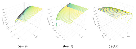
Figure 2. 3D plots of log-likelihood surfaces for the IH parameters.

We now consider the asymptotic normality (AN) of each MLE to construct its corresponding asymptotic confidence interval (ACI), denoted ACI-AN. Accordingly, based on (45)–(47), the $(1-\gamma )100\%$ ACI-AN estimators for $\alpha$, $\beta$, and $\theta$, respectively, are given as follows:

$$\begin{array}{c}\hfill \left(\widehat{\alpha }\mp z_{{\displaystyle \frac{\gamma }{2}}}\sqrt{{\widehat{\sigma }}_{11}}\right),\left(\widehat{\beta }\mp z_{{\displaystyle \frac{\gamma }{2}}}\sqrt{{\widehat{\sigma }}_{22}}\right),\mathrm{and}\left(\widehat{\theta }\mp z_{{\displaystyle \frac{\gamma }{2}}}\sqrt{{\widehat{\sigma }}_{33}}\right),\end{array}$$

(48)

where $z_{{\displaystyle \frac{\gamma }{2}}}$ is an upper limit $\left({\displaystyle \frac{\gamma }{2}}\right)\%$ of the standard Gaussian distribution.

A log-transformed MLE helps ensure that parameters constrained to be positive are not estimated with invalid negative values. By applying a logarithmic transformation, the resulting sampling distribution becomes more stable and approximately symmetric, particularly for small sample sizes. When the ACI is back-transformed, it remains within the valid positive range, thus improving its efficiency; see Meeker and Escobar [19] and Nassar and Elshahhat [20] for additional details. Hence, the NA of the log-MLE is used to construct its corresponding ACI, abbreviated ACI-NL. Accordingly, from (45)–(47), the $(1-\gamma )100\%$ ACI-NL estimators for $\alpha$, $\beta$, and $\theta$ are given as follows:

$$\begin{array}{c}\hfill \widehat{\alpha }\times exp\left(\mp {\displaystyle \frac{z_{\frac{\gamma }{2}}}{\widehat{\alpha }}}\sqrt{{\widehat{\sigma }}_{11}}\right),\widehat{\beta }\times exp\left(\mp {\displaystyle \frac{z_{\frac{\gamma }{2}}}{\widehat{\beta }}}\sqrt{{\widehat{\sigma }}_{22}}\right),\mathrm{and}\widehat{\theta }\times exp\left(\mp {\displaystyle \frac{z_{\frac{\gamma }{2}}}{\widehat{\theta }}}\sqrt{{\widehat{\sigma }}_{33}}\right),\end{array}$$

(49)

respectively.

To get the estimated variances ${\widehat{\sigma }}_{ii},i=1,2,3$ (provided in (48) and (49)), we first obtain six quantities from (44), namely ${\mathcal{I}}_{ij},i,j=1,2,3$, as: 0pt

$${\mathcal{I}}_{11}=-\sum _{i=1}^d{\varrho }_i^{-2}+{\displaystyle \frac{(n-d)}{{\theta }^2}}{\vartheta }_d^{-{\displaystyle \frac{\alpha }{\theta }}}{\xi }_d^{-2}{log}^2\left({\vartheta }_d\right)e^{-{\displaystyle \frac{\beta }{2x_d^2}}},$$

$${\mathcal{I}}_{22}=-\sum _{i=1}^d{x}_i^{-2}{\vartheta }_i^2{\varrho }_i^{-2}+{\displaystyle \frac{(n-d)}{4x_d^4}}{\vartheta }_d^{-{\displaystyle \frac{\alpha }{\theta }}}{\xi }_d^{-2}{e}^{-{\displaystyle \frac{\beta }{2x_d^2}}},$$

$${\mathcal{I}}_{33}=-\beta \sum _{i=1}^d{x}_i^{-3}{\varrho }_i^{-2}+{\displaystyle \frac{2\alpha }{{\theta }^3}}\sum _{i=1}^{d}log\left({\vartheta }_i\right)-{\displaystyle \frac{\alpha }{\theta }}\sum _{i=1}^d{x}_i^{-2}{\vartheta }_i^{-2}-{\displaystyle \frac{\alpha (n-d)}{{\theta }^2}}{\vartheta }_d^{-{\displaystyle \frac{\alpha }{\theta }}}{\xi }_d^{-2}log({\vartheta }_d-1)e^{-{\displaystyle \frac{\beta }{2x_d^2}}},$$

$${\mathcal{I}}_{12}=\sum _{i=1}^d{x}_i^{-1}{\vartheta }_i{\varrho }_i^{-2},$$

$${\mathcal{I}}_{13}=\beta \sum _{i=1}^d{x}_i^{-2}{\varrho }_i^{-2}-{\displaystyle \frac{1}{{\theta }^2}}\sum _{i=1}^{d}log\left({\vartheta }_i\right)+{\displaystyle \frac{1}{\theta }}\sum _{i=1}^d{x}_i^{-1}{\vartheta }_i^{-1}+{\displaystyle \frac{\alpha (n-d)}{{\theta }^2}}{\vartheta }_d^{-{\displaystyle \frac{\alpha }{\theta }}}{\xi }_d^{-1}{e}^{-{\displaystyle \frac{\beta }{2x_d^2}}}\left(log\left({\vartheta }_d\right)-1\right),$$

and

$${\mathcal{I}}_{23}=\sum _{i=1}^d{x}_i^{-2}{\varrho }_i^{-2}-2(n-d)x_d^{-2}{\vartheta }_d^{-{\displaystyle \frac{\alpha }{\theta }}}{\xi }_d^{-1}{e}^{-{\displaystyle \frac{\beta }{2}}},$$

where ${\xi }_d=\left(1-{\vartheta }_d^{-{\displaystyle \frac{\alpha }{\theta }}}{e}^{-{\displaystyle \frac{\beta }{2x_d^2}}}\right).$

Using the invariance property of the MLEs $\widehat{\alpha }$, $\widehat{\beta }$, and $\widehat{\theta }$, the approximate variance–covariance (AVC) matrix, denoted $\Sigma (·)$, is obtained, from which the MLEs of ${\sigma }_{ii}$, for $i=1,2,3$, are derived as follows:

$$\widehat{\Sigma }\left(\widehat{\Omega }\right)={\left[\begin{array}{ccc}{\mathcal{I}}_{11}& & \\ {\mathcal{I}}_{12}& {\mathcal{I}}_{22}& \\ {\mathcal{I}}_{31}& {\mathcal{I}}_{32}& {\mathcal{I}}_{33}\end{array}\right]}_{(\Omega =\widehat{\Omega })}^{-1}=\left[\begin{array}{ccc}{\widehat{\sigma }}_{11}& & \\ {\widehat{\sigma }}_{21}& {\widehat{\sigma }}_{22}& \\ {\widehat{\sigma }}_{31}& {\widehat{\sigma }}_{32}& {\widehat{\sigma }}_{33}\end{array}\right].$$

(50)

To obtain the MLEs, we recommend using the Newton–Raphson (NR) algorithm to solve the likelihood equations. To implement this, after installing the maxLik package in R (version 4.2.2), the MLEs, along with their $(1-\gamma )100\%$ ACIs, for $\alpha$, $\beta$, and $\theta$ can be computed.

4.2. Bayesian Inference

This subsection explores the Bayesian estimators and the associated $(1-\gamma )100\%$ Bayesian credible intervals (BCIs), including highest posterior density (HPD) intervals, based on three independent gamma conjugate priors for $\alpha$, $\beta$, and $\theta$. The gamma distribution is adopted as the prior density because it exhibits flexible shapes depending on the chosen hyperparameters, making it a more suitable prior for model parameters compared to more complex alternatives; see Dey et al. [21] for further discussion. Therefore, gamma priors are employed to ensure proper support for the IH parameters. Hence, the joint prior PDF, denoted ${\rm Y}(·)$, for $\Omega$, up to a proportionality constant, is given by

$${\rm Y}\left(\Omega |\mathbf{x}\right)\propto \prod _{i=1}^3{\lambda }_i^{a_i-1}{e}^{-b_i{\lambda }_i},\alpha ,\beta ,\theta >0,$$

(51)

where $a_i>0$ and $b_i>0$ for $i=1,2,3,$ are the shape and scale hyper-parameters, respectively, of ${\lambda }_1=\alpha$, ${\lambda }_2=\beta$, and ${\lambda }_3=\theta$.

Combining (51) with (42), the joint posterior distribution (say, $\Pi (·)$) of $\alpha$, $\beta$, and $\theta$ becomes

$$\Pi \left(\Omega \right)={\mathcal{P}}^{-1}{\xi }_d^{n-d}{e}^{-\beta {\displaystyle \sum _{i=1}^d}{\displaystyle \frac{1}{2x_i^2}}}\prod _{i=1}^3{\lambda }_i^{a_i-1}{e}^{-b_i{\lambda }_i}\prod _{i=1}^d{\varrho }_i{\vartheta }_i^{-{\displaystyle \frac{\alpha }{\theta }}-1},$$

(52)

and $\mathcal{P}={\int }_0^{\infty }{\int }_0^{\infty }{\int }_0^{\infty }{\rm Y}\left(\Omega \right)·L\left(\mathbf{x}\right|\Omega )\mathrm{d}\alpha \mathrm{d}\beta \mathrm{d}\theta$ is the normalizing term.

The Bayes estimators of $\alpha$, $\beta$, and $\theta$, denoted $\tilde{\alpha }$, $\tilde{\beta }$, and $\tilde{\theta }$, respectively, for a generic function $\phi (\Omega )$ under the squared error loss (SEL) function, are directly given by the posterior mean of $\phi (\Omega )$, as follows:

$$\tilde{\phi }(\Omega )={\mathcal{P}}^{-1}{\int }_0^{\infty }{\int }_0^{\infty }{\int }_0^{\infty }\phi (\Omega )·\Pi \left(\Omega \right)\mathrm{d}\alpha \mathrm{d}\beta \mathrm{d}\theta .$$

(53)

Due to the nonlinear nature of the posterior mean in (53), the marginal posterior PDFs of $\alpha$, $\beta$, and $\theta$ cannot be obtained in closed form. Therefore, Markov chain Monte Carlo (MCMC) methods are recommended to generate posterior samples from (52), evaluate the Bayes estimators of $\alpha$, $\beta$, and $\theta$, and construct their BCI and HPD interval estimates. To implement this, the full conditional distributions of $\alpha$, $\beta$, and $\theta$ derived from (52) are given by:

$${\Pi }_1\left(\alpha |\mathbf{x},\beta ,\theta \right)\propto {\alpha }^{a_1-1}{e}^{-b_1\alpha }{\xi }_d^{n-d}\prod _{i=1}^d{\varrho }_i{\vartheta }_i^{-{\displaystyle \frac{\alpha }{\theta }}-1},$$

(54)

$${\Pi }_2\left(\beta |\mathbf{x},\alpha ,\theta \right)\propto {\beta }^{a_2-1}{e}^{-\beta \left(b_2+{\sum }_{i=1}^d{\displaystyle \frac{1}{2x_i^2}}\right)}{\xi }_d^{n-d}\prod _{i=1}^d{\varrho }_i,$$

(55)

and

$${\Pi }_3\left(\theta |\mathbf{x},\alpha ,\beta \right)\propto {\theta }^{a_3-1}{e}^{-b_3\theta }{\xi }_d^{n-d}\prod _{i=1}^d{\varrho }_i{\vartheta }_i^{-{\displaystyle \frac{\alpha }{\theta }}-1},$$

(56)

respectively.

From (54) and (56), the conditional posterior PDFs of $\alpha$, $\beta$, and $\theta$ do not belong to any standard family of distributions. Using the same TIIC dataset employed in Figure 2, the posterior distributions ${\Pi }_i$ ($i=1,2,3$) of $\alpha$, $\beta$, and $\theta$ are displayed in Figure 3. It reveals that all posterior PDFs of $\alpha$, $\beta$, and $\theta$ exhibit approximately normal behavior. Consequently, the Metropolis–Hastings (M–H) algorithm with a normal proposal distribution is recommended for generating MCMC samples to obtain the Bayes point estimates and their corresponding $(1-\gamma )100\%$ credible intervals for each unknown parameter.

Figure 3. Posterior distribution plots of $\alpha$, $\beta$, and $\theta$.

To perform the M-H algorithm, do the following steps:

Step 1.

Put $i=1$.

Step 2.

Set $({\alpha }^{\left[0\right]},{\beta }^{\left[0\right]},{\theta }^{\left[0\right]})=(\widehat{\alpha },\widehat{\beta },\widehat{\theta })$.

Step 3.

Obtain ${\alpha }^{★}$ from normal proposal distribution $N(\widehat{\alpha },{\widehat{\sigma }}_{11})$.

Step 4.

Obtain ${\eta }_1={\Pi }_1\left({\alpha }^{\left[i\right]}\right|\mathbf{x},{\beta }^{i-1},{\theta }^{i-1})$.

Step 5.

Generate $u_1$ from uniform $U(0,1)$ distribution.

Step 6.

If $u_1⩽min\{1,{\eta }_1\}$, set ${\alpha }^{\left[i\right]}={\alpha }^{*}$ else set ${\alpha }^{\left[i\right]}={\alpha }^{[i-1]}$.

Step 7.

Set $i=i+1$.

Step 8.

Redo Steps 2-7 ${\mathcal{B}}^{•}$ times, burning in ${\mathcal{B}}^{\circ }$, to get $\left({\alpha }^{[{\mathcal{B}}^{\circ }+1]},{\alpha }^{[{\mathcal{B}}^{\circ }+2]},\dots ,{\alpha }^{\left[{\mathcal{B}}^{•}\right]}\right)$.

Step 9.

Find the MCMC point estimate of $\alpha$ through the SEL as:

$$\tilde{\alpha }={\displaystyle \frac{1}{\overline{\mathcal{B}}}}\sum _{i={\mathcal{B}}^{\circ }+1}^{{\mathcal{B}}^{•}}{\alpha }^{\left[i\right]},$$

where $\overline{\mathcal{B}}={\mathcal{B}}^{•}-{\mathcal{B}}^{\circ }$.

Step 10.

Find the $(1-\gamma )100\%$ BCI bounds of $\alpha$ as:

(a)

Sort ${\alpha }^{\left[i\right]}$ for $i={\mathcal{B}}^{\circ }+1,{\mathcal{B}}^{\circ }+2,\dots ,{\mathcal{B}}^{•}$ as:

$$\left({\alpha }_{[{\mathcal{B}}^{\circ }+1]},{\alpha }_{[{\mathcal{B}}^{\circ }+2]},\dots ,{\alpha }_{\left[{\mathcal{B}}^{•}\right]}\right).$$

(b)

The BCI bounds of $\alpha$ take:

$$\left\{{\alpha }_{\left[{\displaystyle \frac{\gamma }{2}}\overline{\mathcal{B}}\right]},{\alpha }_{\left[\left(1-{\displaystyle \frac{\gamma }{2}}\right)\overline{\mathcal{B}}\right]}\right\}.$$

Step 11.

The $100(1-\gamma )\%$ HPD interval of $\alpha$ is computed as follows:

• Use outputs in Step 10 (a).
• Create the HPD interval as:

  $$\left[{\alpha }_{\left[i^{*}\right]},{\alpha }_{\left[i^{*}+\left(1-\gamma \right)\overline{\mathcal{B}}\right]}\right],$$

  where $i^{*}={\mathcal{B}}^{\circ }+1,\dots ,{\mathcal{B}}^{•}$ is determined by

  $${\alpha }_{[i^{*}+\left[(1-\gamma )\overline{\mathcal{B}}\right]]}-{\alpha }_{\left[i^{*}\right]}=\underset{1⩽i⩽\gamma \overline{\mathcal{B}}}{\min }\left\{{\alpha }_{[i+\left[(1-\gamma )\overline{\mathcal{B}}\right]]}-{\alpha }_{\left[i\right]}\right\},$$

  where $\left[i\right]$ refers to the highest integer which not exceed i.

Step 12.

Redo Steps 2–11 for $\beta$ and $\theta$.

5. Monte Carlo Simulations

To examine the performance of the offered estimators of the proposed IH estimators mentioned in earlier sections, in this part, we conduct several Monte Carlo comparisons. To achieve this, we create several TIIC samples using specified configurations of IH parameters $\Omega$ by following the next steps:

Step 1:

Set two sets of IH parameters, namely:

• Set 1: $\mathrm{IH}(0.8,0.5,0.2)$;
• Set 2: $\mathrm{IH}(1.5,2.0,2.5)$.

Step 2:

Fix levels of sample sizes $n(=20,50,80,100,150,200)$.

Step 3:

Generate $u_i\sim U(0,1)$ independently for $i=1,2,\dots ,n$.

Step 4:

Set $X_i=F^{-1}(\Omega ;u_i),i=1,2,\dots ,n$.

Step 5:

Fix levels of failure percentages (FPs) of each n, where $\mathrm{FP}={\displaystyle \frac{d}{n}}\times 100\%$, such as FP $(=50,80,100\%)$.

Step 6:

Perform 5000 replications for each setting.

To get the Bayes estimates and associated 95% BCI/HPD intervals of $\alpha$, $\theta$, or $\beta$, beyond assigning ${\mathcal{B}}^{\circ }$ = 2000 and ${\mathcal{B}}^{•}$ = 12,000, we use two informative prior sets for each parameter group, namely:

• For Set 1:

  –

  Prior-1 (P1): $(a_1,a_2,a_3)=(4,2.5,1)$ and $b_i=5$;

  –

  Prior-2 (P2): $(a_1,a_2,a_3)=(8,5,2)$ and $b_i=10$.

• For Set 2:

  –

  Prior-1 (P1): $(a_1,a_2,a_3)=(7.5,10,12.5)$ and $b_i=5$;

  –

  Prior-2 (P2): $(a_1,a_2,a_3)=(15,20,25)$ and $b_i=10$.

Comparison of the point estimates of $\alpha$ (as an example) is done using their mean squared errors (MSEs) and mean absolute biases (MABs) as:

$$\mathrm{MSE}\left(\check{\alpha }\right)={\displaystyle \frac{1}{1000}}{\sum }_{i=1}^{1000}{\left({\check{\alpha }}^{\left[i\right]}-\alpha \right)}^2,$$

and

$$\mathrm{MAB}\left(\check{\alpha }\right)={\displaystyle \frac{1}{1000}}{\sum }_{i=1}^{1000}\left|{\check{\alpha }}^{\left[i\right]}-\alpha \right|,$$

respectively. Also, the comparison of the interval estimates of $\alpha$ (as an example) is done using their average interval lengths (AILs) and coverage percentages (CP) as follows:

$${\mathrm{AIL}}^{95\%}\left(\alpha \right)={\displaystyle \frac{1}{1000}}{\sum }_{i=1}^{1000}\left(U_{{\widehat{\alpha }}^{\left[i\right]}}-L_{{\widehat{\alpha }}^{\left[i\right]}}\right)$$

and

$${\mathrm{CP}}^{95\%}\left(\alpha \right)={\displaystyle \frac{1}{1000}}{\sum }_{i=1}^{1000}{\mathsf{1}}_{\left(L_{{\widehat{\alpha }}^{\left[i\right]}};U_{{\widehat{\alpha }}^{\left[i\right]}}\right)}\left(\alpha \right),$$

where $\mathsf{1}(·)$ is the indicator function, $L(·)$ and $U(·)$ denote the lower and upper bounds, respectively, of each offered interval estimator.

By installing two $\mathsf{R}$ programming packages, namely ’$\mathtt{maxLik}$’ and ’$\mathsf{coda}$,’ suggested by Henningsen and Toomet [22] and Plummer et al. [23], respectively, the classical and Bayesian calculations, in addition to their interval estimations, are obtained. All software scripts used for these calculations are available upon request. Table 2, Table 3, Table 4, Table 5, Table 6 and Table 7 present the simulated MSE, MAB, AIL, and CP values for the parameters $\alpha$, $\theta$, and $\beta$. The results indicate the following trends:

Table 2. The MSEs (1st Col.) and MABs (2nd Col.) of $\alpha$.

n	FP%	Set 1						Set 2
		MSE			MAB			MSE			MAB
		MLE	Bayes-P1	Bayes-P2	MLE	Bayes-P1	Bayes-P2	MLE	Bayes-P1	Bayes-P2	MLE	Bayes-P1	Bayes-P2
20	50%	0.019	0.016	0.011	0.600	0.198	0.139	0.259	0.174	0.099	0.418	0.282	0.225
50		0.015	0.013	0.009	0.550	0.184	0.110	0.225	0.131	0.076	0.373	0.256	0.188
100		0.011	0.009	0.008	0.525	0.176	0.100	0.195	0.107	0.066	0.315	0.232	0.171
150		0.009	0.008	0.006	0.497	0.156	0.095	0.163	0.096	0.055	0.299	0.213	0.168
200		0.008	0.006	0.002	0.434	0.148	0.089	0.121	0.085	0.044	0.276	0.195	0.158
20	80%	0.015	0.013	0.009	0.550	0.180	0.121	0.229	0.147	0.088	0.373	0.269	0.219
50		0.012	0.010	0.007	0.515	0.176	0.105	0.192	0.120	0.068	0.342	0.235	0.194
100		0.009	0.008	0.006	0.462	0.162	0.094	0.139	0.096	0.053	0.299	0.220	0.164
150		0.007	0.007	0.004	0.392	0.148	0.091	0.108	0.085	0.048	0.275	0.199	0.156
200		0.005	0.003	0.002	0.384	0.140	0.085	0.096	0.074	0.041	0.254	0.177	0.144
20	100%	0.012	0.011	0.007	0.521	0.189	0.115	0.175	0.129	0.081	0.352	0.237	0.212
50		0.011	0.008	0.005	0.499	0.167	0.099	0.119	0.110	0.061	0.313	0.219	0.193
100		0.007	0.007	0.004	0.414	0.156	0.087	0.072	0.086	0.044	0.268	0.210	0.167
150		0.006	0.005	0.003	0.381	0.140	0.081	0.065	0.078	0.039	0.227	0.187	0.149
200		0.004	0.003	0.002	0.378	0.133	0.078	0.054	0.064	0.031	0.231	0.165	0.134

Table 3. The MSEs (1st Col.) and MABs (2nd Col.) of $\theta$.

n	FP%	Set 1						Set 2
		MSE			MAB			MSE			MAB
		MLE	Bayes-P1	Bayes-P2	MLE	Bayes-P1	Bayes-P2	MLE	Bayes-P1	Bayes-P2	MLE	Bayes-P1	Bayes-P2
20	50%	0.275	0.063	0.042	0.430	0.207	0.149	0.836	0.256	0.130	0.900	0.424	0.283
50		0.265	0.052	0.030	0.227	0.174	0.114	0.785	0.237	0.115	0.827	0.399	0.276
100		0.250	0.046	0.025	0.186	0.125	0.108	0.705	0.209	0.095	0.728	0.354	0.254
150		0.225	0.040	0.019	0.144	0.110	0.089	0.655	0.182	0.093	0.696	0.343	0.235
200		0.189	0.037	0.016	0.124	0.098	0.085	0.544	0.179	0.086	0.615	0.331	0.223
20	80%	0.250	0.065	0.035	0.362	0.186	0.139	0.752	0.235	0.127	0.808	0.405	0.277
50		0.225	0.047	0.027	0.180	0.153	0.108	0.673	0.210	0.118	0.731	0.376	0.266
100		0.213	0.042	0.020	0.143	0.110	0.100	0.628	0.188	0.105	0.668	0.341	0.245
150		0.175	0.037	0.016	0.126	0.098	0.081	0.597	0.179	0.094	0.605	0.334	0.224
200		0.147	0.033	0.013	0.110	0.089	0.071	0.482	0.156	0.087	0.552	0.326	0.210
20	100%	0.235	0.057	0.028	0.333	0.170	0.124	0.628	0.216	0.131	0.789	0.389	0.269
50		0.215	0.044	0.022	0.169	0.131	0.102	0.545	0.205	0.119	0.619	0.358	0.242
100		0.159	0.038	0.017	0.126	0.102	0.091	0.483	0.168	0.110	0.577	0.324	0.228
150		0.145	0.032	0.014	0.107	0.091	0.078	0.375	0.158	0.093	0.497	0.304	0.204
200		0.124	0.028	0.011	0.095	0.080	0.064	0.318	0.127	0.088	0.440	0.277	0.185

Table 4. The MSEs (1st Col.) and MABs (2nd Col.) of $\beta$.

n	FP%	Set 1						Set 2
		MSE			MAB			MSE			MAB
		MLE	Bayes-P1	Bayes-P2	MLE	Bayes-P1	Bayes-P2	MLE	Bayes-P1	Bayes-P2	MLE	Bayes-P1	Bayes-P2
20	50%	0.022	0.016	0.014	0.136	0.091	0.068	0.654	0.184	0.124	1.074	0.385	0.299
50		0.019	0.012	0.011	0.096	0.077	0.055	0.592	0.168	0.110	0.823	0.325	0.285
100		0.016	0.011	0.009	0.087	0.061	0.048	0.466	0.140	0.099	0.723	0.312	0.273
150		0.013	0.009	0.008	0.070	0.055	0.041	0.322	0.123	0.085	0.671	0.286	0.255
200		0.011	0.007	0.006	0.065	0.048	0.036	0.216	0.110	0.077	0.517	0.260	0.241
20	80%	0.018	0.014	0.010	0.122	0.086	0.063	0.588	0.178	0.110	0.932	0.335	0.277
50		0.016	0.011	0.009	0.090	0.066	0.049	0.452	0.145	0.100	0.769	0.315	0.262
100		0.013	0.008	0.006	0.079	0.052	0.044	0.366	0.134	0.088	0.670	0.304	0.231
150		0.011	0.006	0.004	0.067	0.047	0.039	0.296	0.110	0.077	0.581	0.276	0.215
200		0.009	0.005	0.003	0.060	0.043	0.034	0.193	0.098	0.066	0.469	0.246	0.207
20	100%	0.016	0.012	0.007	0.113	0.074	0.060	0.473	0.158	0.102	0.831	0.293	0.260
50		0.014	0.007	0.006	0.082	0.058	0.046	0.419	0.140	0.097	0.707	0.286	0.249
100		0.010	0.006	0.005	0.072	0.048	0.040	0.325	0.129	0.078	0.605	0.275	0.220
150		0.008	0.005	0.004	0.061	0.043	0.036	0.249	0.102	0.068	0.522	0.268	0.190
200		0.007	0.004	0.002	0.056	0.040	0.031	0.182	0.088	0.057	0.427	0.226	0.181

Table 5. The AILs (1st Col.) and CPs (2nd Col.) of $\alpha$.

n	FP%	Set 1						Set 2
		ACI-NA		BCI-P1		HPD-P1		ACI-NA		BCI-P1		HPD-P1
		ACI-NL		BCI-P2		HPD-P2		ACI-NL		BCI-P2		HPD-P2
20	50%	1.554	0.732	0.662	0.836	0.868	0.890	3.844	1.024	0.917	0.844	0.846	0.860
		1.787	0.712	0.645	0.832	0.880	0.934	4.093	1.003	0.908	0.825	0.850	0.910
50		1.379	0.564	0.528	0.846	0.876	0.910	3.683	1.004	0.909	0.852	0.848	0.867
		1.644	0.552	0.516	0.840	0.888	0.942	3.763	0.983	0.891	0.833	0.859	0.922
100		1.234	0.478	0.457	0.853	0.880	0.920	3.510	1.004	0.907	0.859	0.852	0.870
		1.415	0.467	0.442	0.848	0.890	0.949	3.626	0.983	0.888	0.840	0.864	0.933
150		1.198	0.421	0.399	0.860	0.889	0.930	3.345	0.892	0.852	0.864	0.858	0.875
		1.240	0.406	0.387	0.850	0.902	0.950	3.510	0.881	0.829	0.845	0.867	0.941
200		1.076	0.377	0.366	0.865	0.902	0.935	3.102	0.874	0.818	0.876	0.870	0.878
		1.180	0.369	0.358	0.855	0.910	0.958	3.365	0.861	0.796	0.857	0.875	0.947
20	80%	1.383	0.714	0.656	0.865	0.885	0.940	3.037	0.872	0.804	0.882	0.867	0.880
		1.466	0.693	0.635	0.860	0.902	0.958	3.176	0.846	0.792	0.862	0.870	0.950
50		1.248	0.555	0.515	0.878	0.892	0.950	2.973	0.818	0.767	0.893	0.875	0.885
		1.370	0.543	0.503	0.878	0.908	0.966	3.087	0.811	0.750	0.873	0.880	0.952
100		1.178	0.450	0.430	0.885	0.900	0.960	2.870	0.780	0.743	0.898	0.885	0.890
		1.216	0.437	0.418	0.880	0.912	0.979	2.947	0.764	0.721	0.878	0.890	0.956
150		0.976	0.396	0.380	0.899	0.905	0.967	2.548	0.779	0.731	0.909	0.890	0.959
		1.175	0.382	0.366	0.890	0.920	0.986	2.795	0.763	0.714	0.889	0.894	0.970
200		0.864	0.354	0.342	0.905	0.910	0.975	2.257	0.769	0.714	0.915	0.895	0.963
		1.070	0.345	0.334	0.896	0.930	0.994	2.683	0.754	0.701	0.895	0.915	0.974
20	100%	1.185	0.707	0.651	0.890	0.910	0.952	2.039	0.733	0.684	0.896	0.905	0.972
		1.252	0.687	0.633	0.875	0.939	0.959	2.380	0.713	0.670	0.876	0.920	0.978
50		1.037	0.547	0.512	0.899	0.913	0.958	1.989	0.723	0.682	0.920	0.900	0.975
		1.195	0.536	0.502	0.886	0.944	0.965	2.196	0.711	0.668	0.900	0.927	0.980
100		0.855	0.445	0.426	0.905	0.923	0.968	1.851	0.712	0.679	0.925	0.910	0.978
		0.943	0.433	0.414	0.895	0.948	0.975	1.986	0.707	0.645	0.905	0.935	0.983
150		0.731	0.393	0.376	0.912	0.940	0.978	1.686	0.681	0.640	0.930	0.920	0.980
		0.824	0.382	0.364	0.910	0.954	0.990	1.758	0.665	0.627	0.910	0.932	0.985
200		0.631	0.352	0.340	0.920	0.950	0.983	1.573	0.671	0.638	0.936	0.924	0.984
		0.755	0.341	0.330	0.930	0.960	0.996	1.632	0.657	0.624	0.915	0.930	0.987

Table 6. The AILs (1st Col.) and CPs (2nd Col.) of $\theta$.

n	FP%	Set 1						Set 2
		ACI-NA		BCI-P1		HPD-P1		ACI-NA		BCI-P1		HPD-P1
		ACI-NL		BCI-P2		HPD-P2		ACI-NL		BCI-P2		HPD-P2
20	50%	1.567	0.790	0.682	0.810	0.818	0.940	1.347	1.121	1.099	0.740	0.784	0.840
		1.834	0.765	0.663	0.800	0.897	0.940	1.543	1.037	1.017	0.728	0.800	0.853
50		1.476	0.789	0.676	0.840	0.857	0.930	1.313	1.113	1.092	0.743	0.798	0.848
		1.655	0.764	0.657	0.820	0.920	0.950	1.486	1.028	1.009	0.733	0.815	0.862
100		1.370	0.786	0.673	0.850	0.859	0.940	1.279	1.112	1.090	0.750	0.810	0.852
		1.410	0.764	0.656	0.830	0.929	0.960	1.398	1.024	1.005	0.738	0.819	0.866
150		1.234	0.708	0.630	0.860	0.876	0.967	1.245	1.094	1.078	0.756	0.817	0.865
		1.383	0.687	0.613	0.830	0.949	0.974	1.327	1.021	1.001	0.741	0.824	0.879
200		1.188	0.707	0.629	0.886	0.889	0.977	1.211	1.092	1.070	0.762	0.820	0.869
		1.266	0.687	0.612	0.837	0.949	0.980	1.260	1.018	0.994	0.747	0.830	0.883
20	80%	0.933	0.705	0.626	0.880	0.893	0.948	1.277	1.098	1.088	0.770	0.832	0.872
		1.093	0.686	0.609	0.860	0.935	0.965	1.426	1.015	0.993	0.755	0.835	0.886
50		0.864	0.699	0.624	0.890	0.897	0.955	1.230	1.088	1.080	0.774	0.840	0.885
		0.985	0.679	0.606	0.870	0.946	0.972	1.384	1.015	0.991	0.767	0.847	0.899
100		0.832	0.699	0.622	0.908	0.904	0.968	1.176	1.087	1.075	0.780	0.850	0.895
		0.910	0.677	0.605	0.873	0.953	0.983	1.275	1.012	0.990	0.770	0.850	0.909
150		0.792	0.697	0.620	0.912	0.909	0.980	1.108	1.086	1.064	0.788	0.854	0.900
		0.831	0.677	0.602	0.880	0.959	0.988	1.236	1.010	0.988	0.780	0.860	0.915
200		0.699	0.691	0.615	0.919	0.910	0.990	1.001	1.081	1.061	0.793	0.860	0.906
		0.783	0.673	0.599	0.889	0.960	0.990	1.138	0.993	0.978	0.785	0.878	0.920
20	100%	0.684	0.667	0.609	0.910	0.920	0.956	1.239	1.094	1.069	0.803	0.860	0.911
		0.751	0.614	0.598	0.880	0.943	0.970	1.349	0.987	0.968	0.790	0.889	0.921
50		0.668	0.662	0.597	0.920	0.925	0.965	1.143	1.085	1.063	0.818	0.870	0.914
		0.722	0.614	0.595	0.890	0.955	0.978	1.322	0.985	0.967	0.812	0.912	0.929
100		0.655	0.635	0.566	0.928	0.960	0.975	1.106	1.061	1.040	0.830	0.921	0.940
		0.693	0.585	0.524	0.905	0.959	0.986	1.228	0.983	0.964	0.827	0.924	0.944
150		0.647	0.626	0.565	0.932	0.970	0.987	1.040	1.059	1.037	0.839	0.927	0.956
		0.659	0.584	0.460	0.912	0.959	0.990	1.141	0.982	0.961	0.835	0.931	0.960
200		0.624	0.625	0.557	0.935	0.974	0.992	0.959	1.052	1.030	0.848	0.932	0.960
		0.631	0.579	0.233	0.921	0.968	0.995	1.106	0.979	0.956	0.841	0.935	0.964

Table 7. The AILs (1st Col.) and CPs (2nd Col.) of $\beta$.

n	FP%	Set 1						Set 2
		ACI-NA		BCI-P1		HPD-P1		ACI-NA		BCI-P1		HPD-P1
		ACI-NL		BCI-P2		HPD-P2		ACI-NL		BCI-P2		HPD-P2
20	50%	0.639	0.443	0.414	0.800	0.810	0.937	1.850	1.258	1.106	0.820	0.844	0.851
		1.126	0.373	0.366	0.787	0.897	0.941	1.977	1.126	0.996	0.812	0.858	0.874
50		0.624	0.426	0.409	0.812	0.840	0.940	1.783	1.248	1.083	0.827	0.855	0.867
		0.878	0.357	0.356	0.798	0.910	0.944	1.906	1.110	0.989	0.820	0.885	0.920
100		0.542	0.402	0.390	0.830	0.850	0.942	1.727	1.224	1.077	0.834	0.881	0.910
		0.795	0.347	0.335	0.808	0.919	0.948	1.865	1.080	0.979	0.828	0.890	0.922
150		0.520	0.383	0.320	0.833	0.860	0.946	1.682	1.197	1.010	0.840	0.888	0.918
		0.692	0.330	0.290	0.818	0.925	0.950	1.823	0.987	0.966	0.834	0.897	0.930
200		0.493	0.324	0.312	0.840	0.880	0.948	1.623	1.187	1.001	0.846	0.895	0.927
		0.636	0.291	0.282	0.824	0.928	0.952	1.801	0.971	0.954	0.838	0.903	0.937
20	80%	0.481	0.321	0.309	0.860	0.880	0.951	1.503	1.176	0.995	0.850	0.903	0.938
		0.952	0.279	0.268	0.815	0.936	0.953	1.777	0.969	0.935	0.842	0.908	0.942
50		0.456	0.287	0.259	0.875	0.894	0.955	1.483	1.156	0.968	0.854	0.906	0.940
		0.781	0.243	0.244	0.835	0.941	0.959	1.742	0.925	0.927	0.848	0.913	0.946
100		0.425	0.276	0.251	0.887	0.900	0.958	1.450	1.136	0.967	0.856	0.912	0.949
		0.742	0.234	0.226	0.859	0.947	0.963	1.703	0.916	0.910	0.851	0.915	0.949
150		0.407	0.257	0.248	0.890	0.905	0.963	1.421	1.115	0.947	0.862	0.916	0.952
		0.673	0.231	0.215	0.868	0.952	0.968	1.697	0.904	0.897	0.856	0.918	0.952
200		0.380	0.231	0.223	0.880	0.915	0.967	1.380	1.085	0.928	0.868	0.920	0.954
		0.617	0.224	0.205	0.874	0.956	0.971	1.622	0.875	0.849	0.862	0.925	0.967
20	100%	0.339	0.226	0.219	0.900	0.910	0.970	1.353	1.053	0.905	0.872	0.925	0.960
		0.510	0.215	0.198	0.890	0.960	0.973	1.589	0.856	0.832	0.867	0.935	0.974
50		0.346	0.213	0.218	0.910	0.920	0.977	1.284	1.049	0.885	0.874	0.931	0.969
		0.492	0.202	0.180	0.890	0.964	0.980	1.518	0.841	0.827	0.870	0.941	0.980
100		0.335	0.206	0.199	0.919	0.925	0.980	1.213	1.028	0.861	0.879	0.938	0.978
		0.449	0.190	0.176	0.905	0.969	0.982	1.452	0.826	0.818	0.871	0.944	0.985
150		0.288	0.185	0.191	0.923	0.930	0.984	1.184	1.009	0.842	0.885	0.942	0.980
		0.411	0.185	0.171	0.910	0.970	0.985	1.414	0.818	0.810	0.876	0.949	0.989
200		0.279	0.172	0.188	0.930	0.948	0.980	1.140	0.999	0.839	0.888	0.947	0.988
		0.314	0.178	0.168	0.917	0.974	0.990	1.339	0.807	0.801	0.879	0.952	0.993

• As the sample size n increases, the precision of all parameter estimates improves. A similar improvement is observed as the fraction of failures (FP%) increases.
• As FP% approaches 100%, all point and interval estimation results become satisfactory, consistent with the asymptotic properties of the estimators.
• In terms of minimum MSE and MAB, Bayesian estimates using informative priors outperform likelihood-based estimates due to the incorporation of prior information.
• Credible intervals (e.g., 95% BCI/HPD) are more reliable than asymptotic intervals (95% ACI-NA/ACI-NL), providing lower AIL values and higher CP values.
• Among the asymptotic intervals, the ACI-NA method performs better than the ACI-NL method, yielding lower AIL and higher CP values.
• Among the credible intervals, HPD intervals outperform BCIs, achieving lower AIL and higher CP values.
• Within the Bayesian approaches, Prior-2 (P2) consistently outperforms Prior-1 (P1) due to its lower prior variance.
• Both prior choices produce consistent parameter estimates; however, Prior-2, being more informative, results in slightly better precision (lower MSE and shorter AILs). The sensitivity to prior specification remains moderate and within acceptable limits, confirming the robustness of the Bayesian estimates.
• As $\alpha$, $\theta$, and $\beta$ increase, the simulated MSE, MAB, and AIL values increase, while the associated CP values decrease.
• Overall, Bayesian estimation with a normal proposal in the Metropolis–Hastings algorithm is recommended for IH parameter estimation.

To visualize the simulation results for $\alpha$, $\theta$, and $\beta$, Figure 4 and Figure 5 display the corresponding outcomes. The patterns observed in Figure 4 and Figure 5 are consistent with the numerical results presented in Table 2, Table 3, Table 4, Table 5, Table 6 and Table 7.

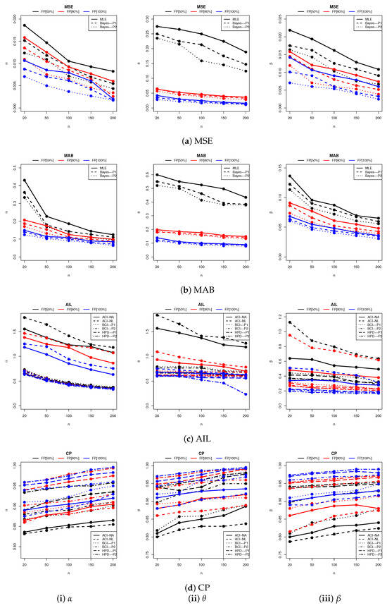
Figure 4. Plots of the simulation results for $\alpha$, $\theta$, and $\beta$ from Set 1.

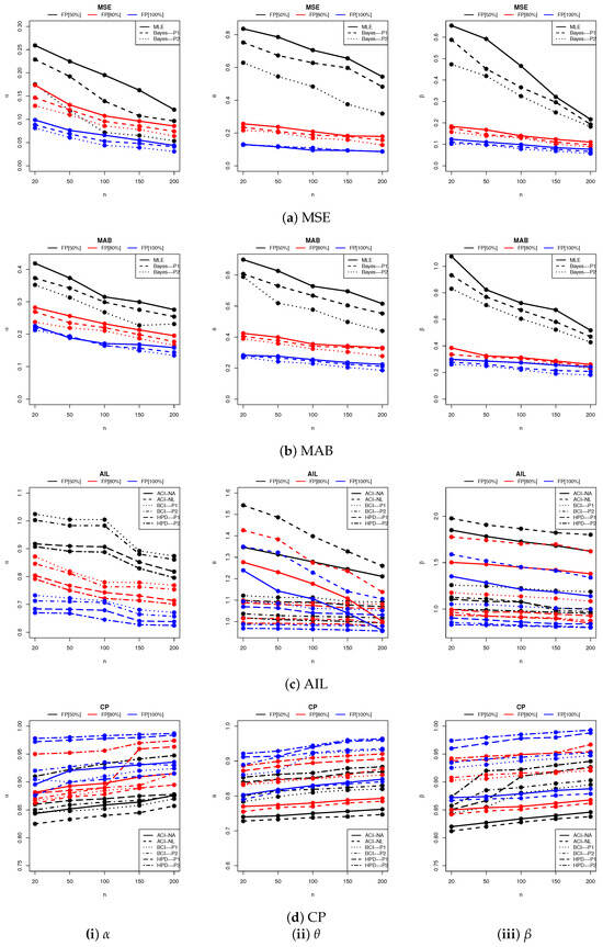
Figure 5. Plots of the simulation results for $\alpha$, $\theta$, and $\beta$ from Set 2.

6. Data Analysis

This section analyzes two real-world datasets from the environmental and pharmacological domains to demonstrate the efficiency and superiority of the IH model and to illustrate the practical relevance of the proposed estimators in real-world scenarios:

Data A:

Maintaining monthly river flows is crucial for preserving aquatic ecosystems, supporting biodiversity, and sustaining water quality for downstream users. It also ensures a reliable water supply for agriculture, industry, and urban consumption, particularly during dry seasons. This dataset represents the minimum monthly water flows (m³/s) of the Piracicaba River, located in São Paulo state, Brazil; see Arshad et al. [24]. The data were obtained from the Department of Water Resources and the Power Agency for Water Resources Management of São Paulo State, covering the period 1960–2014. For computational convenience, all flow measurements ($n=40$) reported in Table 8 have been divided by ten.

Table 8. Two real-word datasets from environmental and pharmacology sciences.

Data	Items
A	1.000	1.286	1.331	1.374	1.592	1.676	1.847	1.847	1.930	1.946
	1.946	1.972	2.103	2.189	2.356	2.429	2.453	2.558	2.755	2.799
	2.919	3.290	3.335	3.362	3.412	3.549	3.604	4.000	4.163	4.410
	4.574	4.700	5.085	5.625	5.927	6.853	8.430	10.633	15.111	37.454
B	0.05	0.06	0.07	0.07	0.07	0.08	0.08	0.08	0.08	0.08
	0.09	0.10	0.10	0.10	0.11	0.11	0.11	0.11	0.12	0.12
	0.12	0.13	0.13	0.16	0.17	0.19	0.20	0.22	0.23	0.24
	0.25	0.30	0.32	0.36	0.37	0.39	0.39	0.40	0.42	0.48
	0.59	0.64	0.64	0.70	0.71	0.78	0.80	0.80	0.81	0.84
	0.89	0.94	1.02	1.03	1.04	1.16	1.39	1.44	1.49	1.50
	1.63	1.85	2.03	2.05	2.31	2.72

Data B:

Plasma concentrations of indomethacin are used to assess the drug’s therapeutic effectiveness and guide dosing to safely manage pain and inflammation. Monitoring these levels also helps minimize the risk of adverse effects, such as gastrointestinal or renal complications, by avoiding toxic concentrations. Table 8 presents a dataset ($n=66$) of plasma indomethacin concentrations (µg/mL); see Arshad et al. [24].

To demonstrate the adaptability of the proposed model, the IH lifetime distribution is compared with eight competing models from the literature:

(1)

Inverted Dagum (ID($\alpha ,\theta ,\beta$)) by Osi et al. [25];

(2)

Generalized inverse Gompertz (GIG($\alpha ,\theta ,\beta$)) by Elshahhat et al. [26];

(3)

Inverted log-logistic (ILL($\alpha ,\theta ,\beta$)) by Leemis [27];

(4)

Inverted Lomax (ILo($\theta ,\beta$)) by Kleiber and Kotz [28];

(5)

Inverted Gompertz (IGo($\theta ,\beta$)) by Eliwa et al. [29];

(6)

Inverted Nadarajah–Haghighi (INH($\theta ,\beta$)) by Tahir et al. [30];

(7)

Inverted exponentiated Pareto (IEP($\theta ,\beta$)) by Abouammoh and Alshingiti [31];

(8)

Exponentiated inverted exponential (EIE($\theta ,\beta$)) by Fatima and Ahmad [32].

To evaluate the goodness-of-fit of the IH model and its competitors, we use several criteria: (i) negative log-likelihood (N-LL), (ii) Akaike information (AI), (iii) consistent Akaike information (CAI), (iv) Bayesian information (BI), (v) Hannan–Quinn information (HQI), and (vi) the Kolmogorov–Smirnov (KS) statistic with its corresponding p-value (see Table 9).

Table 9. Fitting outcomes of the IH model and its competitors from data sets A and B.

Model	$\mathit{\alpha }$	$\mathit{\beta }$	$\mathit{\theta }$	AI	CAI	N-LL	KS	p-Value
				BI	HQI
Data A
IH	0.2568	13.073	10.329	175.88	176.55	84.94	0.0763	0.9740
	1.5915	377.88	3.8028	180.95	177.71
ID	2.0309	7.1426	0.9381	176.06	176.72	85.03	0.0770	0.9729
	0.3931	15.163	1.2148	181.12	177.89
GIG	2.0126	2.7793	1.2957	175.89	176.56	84.94	0.0772	0.9728
	0.7361	1.2521	0.9099	180.96	177.72
ILL	7.1770	2.0224	0.9270	176.05	176.72	85.03	0.0775	0.9733
	7.4643	0.2949	0.5967	181.12	177.88
ILo	-	32.139	0.0830	193.53	193.86	94.77	0.2353	0.0238
	-	34.914	0.0919	196.91	194.75
IGo	-	1.1389	2.7344	177.15	177.48	86.58	0.0932	0.8782
	-	0.3318	0.6464	180.98	178.38
INH	-	20.406	0.0864	180.03	180.36	88.02	0.1657	0.2218
	-	19.354	0.0842	183.41	181.25
IEP	-	3.6764	6.3866	179.28	179.61	87.64	0.0967	0.8484
	-	0.9435	0.9595	182.66	180.51
EIE	-	1.0576	3.3419	189.52	189.85	92.76	0.1754	0.1705
	-	0.4112	0.8951	192.90	190.74
Data B
IH	0.2699	0.4270	0.0145	58.728	59.115	26.364	0.0900	0.6596
	0.0829	0.3173	0.0045	65.297	61.324
ID	1.0858	4.4805	0.0551	64.556	64.943	29.278	0.1225	0.2754
	0.1255	3.4730	0.0508	71.125	67.152
GIG	0.9457	0.1588	0.0289	62.385	62.772	28.193	0.1356	0.1766
	0.2280	0.0637	0.0450	68.954	64.981
ILL	1.8989	1.2521	0.1501	66.527	66.914	30.263	0.1299	0.2154
	0.8463	0.1586	0.0790	73.096	69.122
ILo	-	17.953	0.0111	61.494	61.685	28.747	0.1177	0.3204
	-	14.174	0.0091	65.874	63.225
IGo	-	0.1701	0.0208	60.472	60.663	28.236	0.1420	0.1395
	-	0.0338	0.0295	64.852	62.203
INH	-	1.0701	0.1700	60.926	61.116	28.463	0.1296	0.2179
	-	0.4290	0.1086	65.305	62.656
IEP	-	3.2815	1.2507	65.566	65.756	30.783	0.1452	0.1235
	-	0.6622	0.1547	69.945	67.296
EIE	-	0.1644	0.0905	61.764	61.955	28.882	0.1976	0.0115
	-	0.0820	0.0408	66.144	63.495

For all measures (i)–(vi), the MLEs along with their standard errors (Std. Errs) for $\alpha$, $\beta$, and $\theta$ are computed. In Table 9, the MLEs for $\alpha$, $\beta$, and $\theta$ are reported in the first row, while their corresponding Std. Errs are provided in the second row. Table 9 shows that the IH model outperforms all competing models by achieving the lowest values for all fit metrics and the highest p-value in the KS test.

Figure 6 visualizes the model fits for the IH distribution and its competitors using real datasets A and B, evaluated through four graphical diagnostics: (i) probability–probability (PP) plots, (ii) fitted reliability function (RF) curves, (iii) fitted PDF curves overlaid with histogram-normalized counts (HNC), and (iv) scaled total time on test (TTT) transforms.

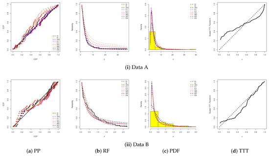
Figure 6. Four fitting diagrams for IH and its competitors from real datasets A and B.

Figure 6a,b for datasets A and B show that the fitted IH distribution closely follows the empirical data points. Figure 6c demonstrate that the fitted IH density curve captures most of the observed histogram for both datasets. Figure 6d (where the theoretical and empirical TTT lines are represented by dashed and solid lines, respectively) confirms that datasets A and B exhibit inverted-bathtub hazard shapes, consistent with the IH failure rate shown in Figure 1. Thus, all visual diagnostics in Figure 6 confirm that the IH lifetime model provides the best fit among the considered alternatives.

Using the complete datasets A and B, in addition to complete sample, two TIIC samples are also considered with sizes $d=20$ and $d=30$ for Data A, and $d=20$ and $d=40$ for Data B. Maximum likelihood and Bayesian methods are employed to obtain point estimates and interval estimates for the parameters $\alpha$, $\beta$, and $\theta$ from all censored samples. The MLEs and Bayesian estimates (along with their Std. Errs) as well as the interval widths (IWs) derived from 95% ACI-NA/ACI-NL and 95% BCI/HPD approaches for $\alpha$, $\beta$, and $\theta$ are summarized in Table 10 and Table 11. For all Bayesian computations, due to the lack of prior knowledge about $\mathrm{IH}(\Omega )$, the hyperparameters $a_i$ and $b_i$ ($i=1,2,3$) are set to $0.0001$, making the gamma priors nearly non-informative. The M–H algorithm is employed with a burn-in period ${\mathcal{B}}^{\circ }=10,000$ and a total of ${\mathcal{B}}^{•}=50,000$ iterations. To assess the existence and uniqueness of the MLEs for $\alpha$, $\beta$, and $\theta$, the corresponding profile log-likelihood functions are plotted in Figure 7 and Figure 8. These plots display clear and well-defined maxima, confirming that the frequentist estimates of $\alpha$, $\beta$, and $\theta$ derived from all samples based on datasets A and B exist and are unique. These graphical findings align with the numerical estimates reported in Table 10 and Table 11, and thus these estimates are used as initial values for subsequent Bayesian computations. Additionally, Figure 7 and Figure 8 present the kernel density estimates (using a Gaussian kernel) alongside trace plots for the 40,000 retained MCMC samples of $\alpha$, $\beta$, and $\theta$ obtained from a representative TIIC sample ($d=20$) for both datasets A and B. The trace plots for each parameter indicate good mixing and suggest convergence of the chains. Moreover, the marginal posterior estimates of $\alpha$, $\beta$, and $\theta$ appear approximately symmetric. These observations further confirm that the chosen burn-in period is sufficient to mitigate the influence of initial values and allow the chains to adequately explore the target posterior distributions.

Table 10. Estimates of $\alpha$, $\beta$, and $\theta$ from Data A.

$(\mathit{n},\mathit{d})$	Par.	MLE		95% ACI-NA			95% BCI
		Bayes		95% ACI-NL			95% HPD
		Est.	Std.Er	Low.	Upp.	IW	Low.	Upp.	IW
(40, 20)	$\alpha$	1.3897	9.3207	0.4527	2.9052	2.4525	1.0462	1.7424	0.6963
		1.4085	0.0206	0.0012	5.2116	5.2103	1.2464	1.5246	0.2782
	$\beta$	10.176	2.9475	4.3993	15.953	11.554	9.9652	10.295	0.3298
		10.075	0.0101	5.7682	17.953	12.184	10.005	10.195	0.1892
	$\theta$	109.95	6.8493	101.80	128.65	26.849	114.96	116.30	1.3431
		115.20	0.0561	100.55	129.46	28.909	115.10	115.30	0.1936
(40, 30)	$\alpha$	0.6965	3.2264	0.1805	1.2581	1.0776	1.0649	1.4603	0.3954
		1.3624	0.1566	0.0079	3.5280	3.5200	1.2693	1.4642	0.1949
	$\beta$	10.393	2.0405	6.3939	14.393	7.9988	9.9955	10.149	0.1948
		10.051	0.0559	7.0735	15.271	8.1977	10.014	10.148	0.1346
	$\theta$	87.191	8.3886	80.750	93.632	12.883	114.81	115.30	0.4900
		115.20	0.0562	78.207	103.28	25.078	115.10	115.23	0.1253
(40, 40)	$\alpha$	0.2568	1.5915	0.0025	0.7608	0.7583	0.1245	0.3173	0.1928
		0.2194	0.0621	0.0015	1.8812	1.8797	0.1222	0.3100	0.1877
	$\beta$	13.073	377.88	9.1905	14.704	5.5137	12.947	13.115	0.1678
		13.046	0.0573	9.8536	16.253	6.3989	12.985	13.147	0.1620
	$\theta$	10.329	3.8028	5.8756	15.782	9.9067	10.209	10.403	0.1942
		10.104	0.0562	5.0197	21.254	16.234	10.018	10.186	0.1687

Table 11. Estimates of $\alpha$, $\beta$, and $\theta$ from Data B.

$(\mathit{n},\mathit{d})$	Par.	MLE		95% ACI-NA			95% BCI
		Bayes		95% ACI-NL			95% HPD
		Est.	Std.Er	Low.	Upp.	IW	Low.	Upp.	IW
(66,20)	$\alpha$	0.0660	0.1597	0.0000	0.3789	0.3789	0.0620	0.0693	0.0073
		0.0020	0.0619	0.0006	7.5843	7.5837	0.0659	0.0698	0.0039
	$\beta$	0.0220	0.0201	0.0000	0.0615	0.0615	0.0183	0.0250	0.0067
		0.0018	0.0184	0.0037	0.1319	0.1282	0.0219	0.0254	0.0035
	$\theta$	0.0716	1.3296	0.0000	2.6775	2.6775	0.0675	0.0750	0.0075
		0.0020	0.0676	0.1801	0.7652	0.5851	0.0715	0.0754	0.0039
(66,40)	$\alpha$	0.6313	0.4802	0.0012	1.5725	1.5713	0.6274	0.6349	0.0075
		0.0020	0.6273	0.0421	2.8038	2.7617	0.6312	0.6351	0.0039
	$\beta$	0.0177	0.0044	0.0090	0.0263	0.0173	0.0140	0.0204	0.0065
		0.0018	0.0141	0.0108	0.0788	0.0680	0.0175	0.0209	0.0035
	$\theta$	2.4306	3.0936	0.0125	8.4939	8.4814	2.4265	2.4340	0.0075
		0.0020	2.4267	2.1006	2.5495	0.4488	2.4306	2.4346	0.0040
(66,66)	$\alpha$	0.2699	0.2879	0.0000	0.8342	1.1286	0.2652	0.2725	0.0073
		0.0028	0.2652	0.0734	2.1840	2.1106	0.2685	0.2731	0.0046
	$\beta$	0.4270	0.5633	0.0000	1.5310	2.2081	0.4189	0.4239	0.0050
		0.0063	0.4189	0.4038	0.4567	0.0528	0.4209	0.4245	0.0036
	$\theta$	0.0145	0.0671	0.0000	0.1460	0.2630	0.0122	0.0181	0.0060
		0.0019	0.0116	0.0074	0.3962	0.3888	0.0156	0.0183	0.0027

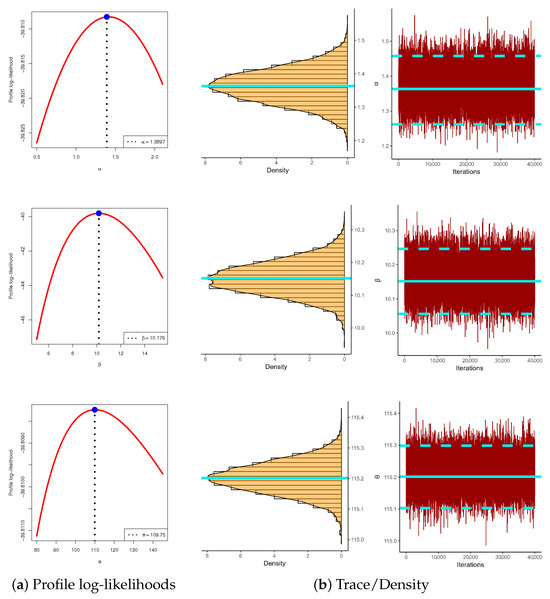
Figure 7. Existences and convergence plots of $\alpha$ (top), $\beta$ (middle), and $\theta$ (bottom) from Data A.

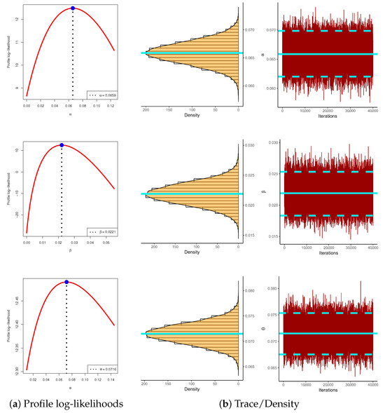
Figure 8. Existences and convergence plots of $\alpha$ (top), $\beta$ (middle), and $\theta$ (bottom) from Data B.

Overall, the results from the environmental and pharmacological case studies demonstrate the flexibility and efficiency of the proposed IH lifetime model in capturing diverse failure behaviors across different scenarios. Compared to eight widely used lifetime models with varying hazard rate structures, the IH model consistently provides the best fit, establishing it as an effective and practical tool for real-world applications. For reproducibility, Appendix B provides the R scripts implementing the main IH functions used in the real-data analyses.

7. Limitations

Despite the promising results and practical importance of the IH model, which shows great flexibility and robust performance in modeling lifetime data, this section provides some limitations to the current study, such as:

• First, the current formulation focuses on univariate lifetime distributions and does not yet account for multivariate extensions or covariate-dependent reliability frameworks, which are often relevant in complex engineering and biomedical applications.
• Second, while Bayesian estimation was successfully implemented, the choice of prior distributions remains a critical factor; although nearly non-informative priors were adopted in this study, further investigation into the sensitivity of the model to alternative informative priors is warranted.
• Third, the simulation experiments and real-data analyses were conducted for selected sample sizes and censoring schemes, and thus the findings may not fully generalize to all experimental designs, particularly under extreme censoring.
• Finally, the comparative study was limited to eight well-known lifetime models; additional benchmarking against more recent flexible distributions could provide a deeper assessment of the IH model’s relative performance.

8. Conclusions

This study introduced the inverted Hjorth (IH) distribution as a flexible alternative to model lifetime data with upside-down bathtub-shaped hazard rates, which are particularly relevant for reliability prediction and maintenance planning. Several analytical properties, including the moment-generating function, quantiles, mean residual life, and order statistics, were derived. Parameter estimation was addressed using both maximum likelihood and Bayesian approaches under Type-II censoring, and two forms of asymptotic confidence intervals and Bayesian credible intervals (BCI and HPD) were proposed. Through extensive Monte Carlo simulations, we observed that MLEs perform reliably for large and complete samples but lose accuracy under heavy censoring or small sample sizes. In contrast, Bayesian estimators, especially with informative priors, demonstrated improved robustness, lower error measures, and more reliable coverage. Bayesian credible intervals were generally shorter and provided better coverage than traditional asymptotic intervals. The practical relevance of the IH model was validated through two real-world datasets: minimum monthly water flows of the Piracicaba River in São Paulo State and plasma concentrations of indomethacin. In both cases, the IH model outperformed eight well-known competing lifetime models, highlighting its superior flexibility and effectiveness. Overall, the IH distribution serves as a valuable tool for modeling complex lifetime behaviors under censoring and limited data conditions. Future work may extend this model to multivariate settings, regression-based lifetime analyses, and more complex real-world reliability problems.

References

- Hjorth, U. A reliability distribution with increasing, decreasing, constant and bathtub-shaped failure rates. Technometrics 1980, 22, 99–107. [Google Scholar] [CrossRef]
- Haj Ahmad, H.; Elshahhat, A. A New Hjorth Distribution in Its Discrete Version. Mathematics 2025, 13, 875. [Google Scholar] [CrossRef]
- Nadarajah, S. Bathtub-shaped failure rate functions. Qual. Quant. 2009, 43, 855–863. [Google Scholar] [CrossRef]
- Rastogi, M.K.; Tripathi, Y.M.; Wu, S.J. Estimating the parameters of a bathtub-shaped distribution under progressive type-II censoring. J. Appl. Stat. 2012, 39, 2389–2411. [Google Scholar] [CrossRef]
- Jiang, R. A new bathtub curve model with a finite support. Reliab. Eng. Syst. Saf. 2013, 119, 44–45. [Google Scholar] [CrossRef]
- Pushkarna, N.; Saran, J.; Verma, K. Progressively Type-II right censored order statistics from Hjorth distribution and related inference. Stat. Optim. Inf. Comput. 2020, 8, 481–498. [Google Scholar] [CrossRef]
- Elshahhat, A.; Nassar, M. Bayesian survival analysis for adaptive Type-II progressive hybrid censored Hjorth data. Comput. Stat. 2021, 36, 1965–1990. [Google Scholar] [CrossRef]
- Bicer, H.D.; Bicer, C.; Bakouch, H.S.H. A geometric process with Hjorth marginal: Estimation, discrimination, and reliability data modeling. Qual. Reliab. Eng. Int. 2022, 38, 2795–2819. [Google Scholar] [CrossRef]
- Lehmann, E.L.; Shaffer, J.P. Inverted distributions. In Selected Works of EL Lehmann; Springer: Boston, MA, USA, 2011; pp. 833–836. [Google Scholar]
- Sharma, V.K.; Singh, S.K.; Singh, U.; Agiwal, V. The inverse Lindley distribution: A stress-strength reliability model with application to head and neck cancer data. J. Ind. Prod. Eng. 2015, 32, 162–173. [Google Scholar] [CrossRef]
- Nguyen, H.C.; Zecchina, R.; Berg, J. Inverse statistical problems: From the inverse Ising problem to data science. Adv. Phys. 2017, 66, 197–261. [Google Scholar] [CrossRef]
- Tomer, S.K.; Panwar, M.S. A review on Inverse Maxwell distribution with its statistical properties and applications. J. Stat. Theory Pract. 2020, 14, 33. [Google Scholar] [CrossRef]
- Choudhary, N.; Tyagi, A.; Singh, B. A flexible bathtub-shaped failure time model: Properties and associated inference. Statistica 2021, 81, 65–92. [Google Scholar]
- Nayal, A.S.; Ramos, P.L.; Tyagi, A.; Singh, B. Improving inference in exponential logarithmic distribution. Commun. Stat.-Simul. Comput. 2024, 99, 1–25. [Google Scholar] [CrossRef]
- Alqasem, O.A.; Nassar, M.; Abd Elwahab, M.E.; Elshahhat, A. A new inverted Pham distribution for data modeling of mechanical components and diamond in South-West Africa. Phys. Scr. 2024, 99, 115268. [Google Scholar] [CrossRef]
- Singh, B.; Tyagi, S.; Singh, R.P.; Tyagi, A. Modified Topp-Leone Distribution: Properties, Classical and Bayesian Estimation with Application to COVID-19 and Reliability Data. Thail. Stat. 2025, 23, 72–96. [Google Scholar]
- Pavia, J.M.; Pavia, M.J.M. Package ‘GoFKernel’. Econom. Theory 2022, 10, 316–356. [Google Scholar]
- Elshahhat, A.; El-Sherpieny, E.S.A.; Hassan, A.S. The Pareto–Poisson Distribution: Characteristics, Estimations and Engineering Applications. Sankhya A 2023, 85, 1058–1099. [Google Scholar] [CrossRef]
- Meeker, W.Q.; Escobar, L.A. Statistical Methods for Reliability Data; Wiley: New York, NY, USA, 1998. [Google Scholar]
- Nassar, M.; Elshahhat, A. Estimation procedures and optimal censoring schemes for an improved adaptive progressively type-II censored Weibull distribution. J. Appl. Stat. 2024, 51, 1664–1688. [Google Scholar] [CrossRef] [PubMed]
- Dey, S.; Elshahhat, A.; Nassar, M. Analysis of progressive type-II censored gamma distribution. Comput. Stat. 2023, 38, 481–508. [Google Scholar] [CrossRef]
- Henningsen, A.; Toomet, O. maxLik: A package for maximum likelihood estimation in R. Comput. Stat. 2011, 26, 443–458. [Google Scholar] [CrossRef]
- Plummer, M.; Best, N.; Cowles, K.; Vines, K. coda: Convergence diagnosis and output analysis for MCMC. R News 2006, 6, 7–11. [Google Scholar]
- Arshad, M.Z.; Iqbal, M.Z.; Al Mutairi, A. A comprehensive review of datasets for statistical research in probability and quality control. J. Math. Comput. Sci. 2021, 11, 3663–3728. [Google Scholar] [CrossRef]
- Osi, A.A.; Sabo, S.A.; Musa, I.Z. Inverted dagum distribution: Properties and application to lifetime dataset. Reliab. Theory Appl. 2024, 19, 595–604. [Google Scholar]
- Elshahhat, A.; Aljohani, H.M.; Afify, A.Z. Bayesian and classical inference under Type-II censored samples of the extended inverse Gompertz distribution with engineering applications. Entropy 2021, 23, 1578. [Google Scholar] [CrossRef]
- Leemis, L.M. Log-logistic distribution. In Univariate Distribution Relationships; Department of Mathematics, The College of William and Mary: Williamsburg, VA, USA, 2008. [Google Scholar]
- Kleiber, C.; Kotz, S. Statistical Size Distributions in Economics and Actuarial Sciences; Wiley and Sons, Inc.: Hoboken, NJ, USA, 2003. [Google Scholar]
- Eliwa, M.S.; El-Morshedy, M.; Ibrahim, M. Inverse Gompertz distribution: Properties and different estimation methods with application to complete and censored data. Ann. Data Sci. 2019, 6, 321–339. [Google Scholar] [CrossRef]
- Tahir, M.H.; Cordeiro, G.M.; Ali, S.; Dey, S.; Manzoor, A. The inverted Nadarajah–Haghighi distribution: Estimation methods and applications. J. Stat. Comput. Simul. 2018, 88, 2775–2798. [Google Scholar] [CrossRef]
- Abouammoh, A.M.; Alshingiti, A.M. Reliability estimation of generalized inverted exponential distribution. J. Stat. Comput. Simul. 2009, 79, 1301–1315. [Google Scholar] [CrossRef]
- Fatima, K.; Ahmad, S.P. The Exponentiated Inverted Exponential Distribution. J. Appl. Inf. Sci. 2017, 5, 35–41. [Google Scholar]
Disclaimer/Publisher’s Note: The statements, opinions and data contained in all publications are solely those of the individual author(s) and contributor(s) and not of MDPI and/or the editor(s). MDPI and/or the editor(s) disclaim responsibility for any injury to people or property resulting from any ideas, methods, instructions or products referred to in the content. |
© 2025 by the authors. Licensee MDPI, Basel, Switzerland. This article is an open access article distributed under the terms and conditions of the Creative Commons Attribution (CC BY) license (https://creativecommons.org/licenses/by/4.0/).