Article

Symmetric Versus Asymmetric Transformer Architectures for Spatio-Temporal Modeling in Effluent Wastewater Quality Prediction

1
Jiangsu Co-Innovation Center of Efficient Processing and Utilization of Forest Resources, Nanjing Forestry University, Nanjing 210037, China
2
College of Information Science and Technology & Artificial Intelligence, Nanjing Forestry University, Nanjing 210037, China
*
Author to whom correspondence should be addressed.
Symmetry 2025, 17(8), 1322; https://doi.org/10.3390/sym17081322
Submission received: 23 May 2025 / Revised: 22 July 2025 / Accepted: 1 August 2025 / Published: 14 August 2025
(This article belongs to the Special Issue Advances in Machine Learning and Symmetry/Asymmetry)

Abstract

Accurate prediction of effluent quality indicators is essential for ensuring stable operation and regulatory compliance in wastewater treatment plants. However, the inherent spatial distribution and temporal fluctuations of wastewater processes present significant challenges for modeling. In this study, we propose a dynamic multi-scale spatio-temporal Transformer (DMST-Transformer) with a symmetric architecture to enhance prediction accuracy in complex wastewater systems. Unlike conventional asymmetric designs, the DMST-Transformer extracts spatial and temporal features in parallel using a spatial graph convolutional network and a multi-scale self-attention mechanism coupled with a dynamic self-tuning module. The model is evaluated on a full-process dataset collected from a municipal wastewater treatment plant, with biochemical oxygen demand selected as the target indicator. Experimental results on test data show that the DMST-Transformer achieves a coefficient of determination of 0.93, root mean square error of 1.40 mg/L, and mean absolute percentage error of 6.61%, outperforming classical models such as linear regression, partial least squares, and graph convolutional networks, as well as advanced deep learning baselines including Transformer and ST-Transformer. Ablation studies confirm the complementary effectiveness of the spatial and temporal modules, and computational time comparisons demonstrate the model’s suitability for real-time applications. These results validate the practical potential of the DMST-Transformer for robust effluent quality monitoring in wastewater treatment plants. Future research will focus on scaling the model to larger and more diverse datasets, extending it to predict additional water quality indicators, and deploying it in real-time environmental monitoring systems to support intelligent water resource management.

1. Introduction

As industrialization progresses, the challenge of achieving high-efficiency wastewater treatment with limited resources has become increasingly critical. Effluent quality indicators in wastewater treatment plants (WWTPs) are subject to increasingly stringent standards, yet their accurate measurement often involves significant time delays, limiting real-time responsiveness [1]. Among these indicators, biochemical oxygen demand (BOD) is widely used to assess pollutant levels [2], but remains difficult to measure in a timely and accurate manner due to the limitations of biochemical assays and the insufficient reliability of hardware sensors [3]. These limitations affect the development and optimization of wastewater treatment control systems [4].
To address this, prediction models based on data analysis have been explored [5]. Conventional approaches include mechanistic and data-driven methods [6,7], such as linear regression (LR), support vector regression [8], regression tree [9], and time series models [10]. While these methods have achieved moderate success, they typically require extensive feature engineering [11]. In contrast to structured data like images or speech, WWTP datasets often feature complex multivariate structures, making effective feature extraction particularly challenging.
Among traditional machine learning methods, partial least squares (PLS) effectively addresses multicollinearity and reduces dimensionality by projecting input variables onto latent components that are most relevant to the target output, making it widely applicable in wastewater prediction tasks [12,13]. However, it remains limited in capturing complex nonlinear and dynamic spatio-temporal dependencies inherent in wastewater treatment processes, motivating the need for more expressive modeling frameworks [14].
Deep learning has driven breakthroughs in environmental monitoring and industrial process control by enabling automatic feature extraction through neural network architectures [15]. Convolutional neural networks (CNNs) and long short-term memory (LSTM) have been widely adopted to learn spatial and temporal features, reducing the need for manual engineering [16]. In wastewater treatment, Li et al. combined CNN and LSTM with attention to predict chemical oxygen demand [17], while Xie et al. used a variational autoencoder to address LSTM-induced information loss [18]. These models improved prediction accuracy, especially when enhanced with attention mechanisms [19]. However, CNN and LSTM still process spatial and temporal dependencies in isolation, limiting their effectiveness under complex wastewater conditions. Most existing approaches process spatial and temporal information in a fixed order, limiting the flexibility of cross-dimensional interaction and potentially reducing their effectiveness in highly dynamic wastewater systems [20].
To address these challenges, the Transformer model introduced by Vaswani et al. employs multi-head self-attention (MHA) to capture long-term dependencies across time sequences, achieving better scalability and accuracy [21]. These characteristics make the Transformer suited for wastewater datasets, as its non-recurrent architecture and positional encoding enable efficient and accurate modeling of temporal sequences [22]. Recent studies have demonstrated the efficacy of Transformer-based architectures for prediction in environmental domains. Chen et al. integrated CNN with Transformer layers to enhance ozone prediction by combining local and global features [23], and Zhang et al. proposed a sparse attention-based Transformer for PM2.5 forecasting, achieving improved accuracy and reduced computational cost across diverse datasets [24].
Despite their strengths in temporal modeling, standard Transformers lack mechanisms for capturing spatial dependencies—an essential aspect in wastewater treatment processes with spatially distributed monitoring units. To overcome this, a spatio-temporal Transformer (ST-Transformer) has been developed to jointly learn spatial and temporal dependencies by extending the multi-head self-attention mechanism [25]. It is able to compute parallel attention across multiple heads, embedding temporal sequences and spatial relationships simultaneously [26,27]. This integrated design has shown strong performance in environmental applications; for instance, ST-Transformers have been applied to wildfire-related PM2.5 prediction, where accurate modeling of both temporal dynamics and spatial variations is critical [28].
Although effective in modeling spatio-temporal data, the ST-Transformer still faces limitations. It processes temporal and spatial features sequentially, leading to potential information loss and weak feature fusion. Its fixed processing order limits flexibility in capturing complex interactions, and it lacks explicit spatial structure modeling, relying solely on attention to infer dependencies. To overcome these issues, spatial graph convolutional networks (SGCNs) have been applied to explicitly model spatial correlations, especially useful in wastewater systems with distributed treatment units [29]. By aggregating information from neighboring data points, SGCNs effectively capture spatial variations, making them a valuable complement to ST-Transformers when spatial relationships are critical. These findings highlight the need for a more advanced architecture that enables efficient and balanced fusion of spatial and temporal features. In particular, a symmetric design that models both dimensions in parallel can avoid sequential bias and preserve more information. Theoretically, such architectures support simultaneous learning across domains, facilitating better cross-dimensional interaction and potentially improving computational efficiency by reducing bottlenecks caused by fixed processing orders [30].
To further address temporal fusion and adaptability concerns, we incorporate a multi-scale self-attention (MSSA) module followed by a dynamic self-tuning (DST) mechanism to enhance temporal modeling capabilities and dynamic responsiveness.
In this study, we introduce the dynamic multi-scale spatio-temporal Transformer (DMST-Transformer) model, which combines SGCN, MSSA, and DST mechanisms to effectively model both spatial and temporal dependencies. The DMST-Transformer adopts a symmetric design that processes spatial and temporal features in parallel, providing a more balanced approach to spatio-temporal modeling in wastewater treatment applications.
To validate its effectiveness, we conduct comparative experiments against representative baselines, including single models (LR, PLS, Transformer, GCN) and the hybrid model (ST-Transformer). Additionally, ablation experiments are conducted by removing key components from the DMST-Transformer to evaluate the individual contributions of each module. The key contributions of this study are as follows:
(1)
The integration of the MSSA mechanism, which utilizes varying dilation rates to capture short-term, medium-term, and long-term temporal dependencies in wastewater datasets, leveraging a multi-head attention structure to process different temporal scales in parallel;
(2)
The incorporation of SGCN to explicitly model spatial relationships between monitoring locations, enhancing the model’s ability to handle spatial variations and interactions;
(3)
The introduction of a symmetric architecture that processes spatial and temporal features in parallel, ensuring equal importance to both aspects and enabling more effective feature fusion;
(4)
The validation of the DMST-Transformer framework using a full-process wastewater treatment dataset, demonstrating superior performance in prediction accuracy and robustness compared to traditional deep learning models.

2. Materials and Methods

2.1. Data Structure and Temporal Encoding

2.1.1. Spatio-Temporal Data Structure

Wastewater treatment processes generate complex multivariate time-series data with intricate temporal and spatial characteristics. The input data represents historical observations from multiple monitoring stations across the treatment system, forming a temporal window of length L:
X t = { x 1 , x 2 , , x L }
where xt contains observations at time step t from all monitoring locations. These observations capture various process variables and effluent quality indices that interact in complex ways throughout the treatment process.
To clarify the spatial dimension, we define each monitoring location as corresponding to a functional unit within the wastewater treatment system. Specifically, variables are recorded across major physical locations such as sludge and effluent. Each location includes several variables that reflect its unique process characteristics. Finally, these distributed points form the spatial structure of the dataset, which is further detailed in the spatial modeling methods described in Section 2.2. And specific information on monitoring positions is provided in Section 3.1.

2.1.2. Temporal Encoding

By refining the positional encoding concept from the original Transformer, we develop dedicated temporal encoding tailored to wastewater treatment data. Unlike standard embedding methods, it inherently preserves the sequential order and captures key temporal patterns. This encoding approach helps the model distinguish between different time steps and recognize the periodic patterns common in wastewater treatment operations.
The temporal encoding uses sinusoidal functions to create unique representations for each position in the sequence while maintaining consistent relative relationships between time steps:
P E ( p o s , 2 i ) = sin p o s 1000 0 2 i d m o d e l
P E ( p o s , 2 i + 1 ) = cos p o s 1000 0 2 i d m o d e l
where pos represents the position index within the input time series, i is the dimension index, and dmodel is the model’s embedding dimension. This encoding approach enables the model to effectively generalize to sequence lengths not encountered during training, which is particularly valuable for wastewater treatment applications where monitoring periods may vary.
The resulting temporal features carry rich information about the sequential order and evolution patterns in the data, providing a solid foundation for the subsequent modeling stages. This encoding mechanism provides essential temporal context for predicting effluent quality indicators.

2.2. Spatial Representation Methods

In spatio-temporal modeling of wastewater treatment processes, effective representation of spatial relationships is crucial for accurate prediction. As wastewater treatment involves complex interactions between multiple variables across different monitoring locations, the choice of spatial representation method significantly impacts the model’s ability to capture these relationships accurately. In the subsequent study, two representative spatial modeling strategies are considered: a conventional embedding-based method and a graph-based approach, each offering different capabilities in characterizing spatial dependencies.

2.2.1. Traditional Embedding-Based Representation

The most straightforward approach to spatial representation is conventional spatial embedding, which maps the original input features through a trainable embedding matrix:
H spatial = X W spatial
where Wspatial is a fully connected weight matrix that learns the spatial representation of each variable through training. This approach has been widely used in various spatio-temporal modeling tasks due to its simplicity and computational efficiency. By transforming input features into a higher-dimensional space, it can capture certain basic spatial characteristics of the data.
However, as wastewater treatment processes become more complex with numerous interconnected variables, the limitations of traditional spatial embedding become increasingly apparent. While enhancing individual variable expressiveness, traditional embedding lacks the structural capacity to capture inter-variable dependencies, which is an essential aspect of wastewater systems.

2.2.2. Graph-Based Representation with SGCN

To model spatial dependencies among variables, this study employs a spatial graph convolutional network (SGCN), which constructs a graph-based representation of inter-variable relationships within the wastewater treatment system. In this formulation, variables are treated as interconnected nodes that reflect the physical and biochemical interactions present in the process. The resulting structure is formalized as an undirected graph:
G   =   V ,   E
where V denotes the set of spatial nodes (i.e., monitoring variables or locations), and E represents the set of edges that encode their spatial or functional connectivity.
The key advantage of SGCN is its ability to dynamically update feature representations by aggregating information from neighboring nodes. The forward propagation in an SGCN layer is formulated as follows:
H ( l + 1 ) = σ A H ( l ) W ( l )
where H(l) is the input feature matrix at the l-th layer, W(l) is the learnable weight matrix, σ(·) is the ReLU activation function, and A is the adjacency matrix encoding spatial connections among variables.
An important challenge in applying SGCN to wastewater treatment is determining the initial connectivity structure. Unlike some domains where physical connections are well-defined, the exact spatial relationships between sensors in wastewater systems are often ambiguous and evolve with operational conditions. We address this by initializing the adjacency matrix as an identity matrix:
A ^ = I R M × M
where I is the identity matrix and M represents the number of monitoring variables. This initialization treats all nodes as initially independent, enabling the model to adaptively learn meaningful connectivity patterns from the data during training.
The SGCN module models spatial dependencies by aggregating features from neighboring nodes within a learned graph structure. Figure 1 illustrates the SGCN module structure and its operation on monitoring variables, showing how the graph representation and identity matrix initialization work together in the forward propagation process.

2.3. Multi-Scale Self-Attention and Dynamic Self-Tuning

Wastewater treatment processes involve complex temporal dependencies across multiple time scales, which stem from operational cycles, periodic loading fluctuations, and long-term seasonal changes. To effectively capture these dynamics, we incorporate a multi-scale self-attention (MSSA) module followed by a dynamic self-tuning (DST) mechanism, aimed at enhancing temporal modeling capabilities and dynamic responsiveness.
The MSSA mechanism draws inspiration from recent advances in multi-resolution Transformers such as Pathformer and Scaleformer [31], and utilizes attention dilation or multi-resolution projections to capture short-, medium-, and long-term temporal dependencies in parallel.
The input to the MSSA module is the temporal features Htemporal obtained from the temporal encoding stage. The basic attention operation for input features is defined by the scaled dot-product attention formula:
Attention ( Q , K , V ) = softmax Q K T d k V
where Q, K, and V are query, key, and value matrices, respectively, and dk is the dimensionality of the key vector.
Multi-head attention extends this operation by projecting the input Htemporal into multiple subspaces, enabling parallel attention across different representations:
head i = Attention ( H t e m p o r a l W i Q , H t e m p o r a l W i K , H t e m p o r a l W i V )
MHA ( H t e m p o r a l ) = Concat ( head 1 , head 2 , , head h ) W O
where W i Q , W i K , and W i V are learnable projection matrices for each attention head, and W O is the output projection matrix.
Building upon this foundation, the MSSA mechanism applies multi-head attention with different dilation rates to capture temporal dependencies at various scales:
H ( k ) = MHA ( k ) ( H temporal ; D k )
where MHA(k) represents the multi-head attention mechanism with dilation rate k from the set D = {1, 2, 4}. These three dilation rates correspond to distinct temporal granularities: short-term patterns (capturing immediate fluctuations), medium-term cycles (modeling daily operational patterns), and long-term trends (identifying weekly patterns or slow-evolving dynamics) in wastewater treatment processes.
The multi-scale temporal representation is then obtained by concatenating the outputs from these three temporal scales:
H MSSA = Concat ( [ H ( 1 ) , H ( 2 ) , H ( 3 ) ] )
where Concat(·) denotes the operation that concatenates the features from different dilation rates along the feature dimension, resulting in a richer representation that captures temporal patterns at multiple scales simultaneously.
To further enhance temporal adaptability, we incorporate a dynamic self-tuning (DST) mechanism after the MSSA module. DST applies a learnable gating function, implemented through Sigmoid activation, to dynamically reweight outputs based on contextual dependencies:
α = σ ( H MSSA W DST )
where σ(·) represents the Sigmoid activation function, and WDST is a trainable weight matrix.
The final gated output is expressed as a simple element-wise multiplication:
H DST = α H MSSA
where denotes element-wise multiplication used for gated weighting fusion. This mechanism preserves the information foundation of all scale features while adaptively enhancing attention to critical time periods and variables through the gating mechanism.
The MSSA and DST mechanisms are jointly incorporated to model temporal dependencies across multiple scales and to adaptively reweight the outputs based on temporal correlation patterns observed in the input data. MSSA captures temporal patterns using parallel attention branches with different dilation rates, while DST applies a gating function to modulate the contribution of each scale during training.

2.4. Benchmark Architecture: Asymmetric ST-Transformer Architecture

The asymmetric spatio-temporal Transformer (ST-Transformer) architecture processes spatial and temporal features sequentially, following a specific order of operations. This model adopts an encoder-only Transformer architecture, which differs from the traditional encoder-decoder Transformer design. The encoder-only design suits time series regression tasks, which aim to map input sequences to target values without generating output sequences. This choice reduces complexity while preserving the ability to model temporal dependencies through self-attention.
First, the input data undergoes temporal encoding as described in Section 2.1, where temporal features are extracted and encoded using sinusoidal positional encoding. This process captures the temporal dependencies and periodic patterns in the data, resulting in the temporal embeddings Htemporal. After the temporal encoding stage, the temporal embeddings are passed through the spatial embedding stage, where traditional spatial embedding is applied as described in Section 2.2. The input features are mapped through a trainable spatial embedding matrix to obtain the spatially embedded representation Hspatial.
The temporal and spatial features are then fused using element-wise addition to obtain a unified spatio-temporal representation:
H fusion = H spatial + H temporal
The fused representation Hfusion is fed into the Transformer encoder composed of multiple stacked layers. Each encoder layer contains two main components: a multi-head self-attention mechanism and a feed-forward neural network, both followed by residual connections and layer normalization to ensure stable training. For the l-th encoder layer, the multi-head attention output can be expressed as follows:
Z ( l ) = LayerNorm ( H ( l 1 ) + MultiHead ( H ( l 1 ) ) )
where H(l−1) is the output from the previous layer (for l = 1, H(0) = Hfusion), and MultiHead(·) represents the standard multi-head attention computation.
The feed-forward network then processes this intermediate representation:
H ( l ) = LayerNorm ( Z ( l ) + FFN ( Z ( l ) ) )
where FNN(·) is a position-wise feed-forward network consisting of two linear transformations with a ReLU activation in between:
FFN ( x ) = ReLU ( x W 1 + b 1 ) W 2 + b 2
where W1 and W2 are weight matrices for the first and second linear transformations, respectively, and b1 and b2 are the corresponding bias vectors.
After L encoder layers, the final output H(L) contains enriched spatio-temporal features. This output is passed to a linear projection layer to produce the final prediction:
Y ^ = Dense ( H ( L ) )
where Dense(·) represents a fully connected linear operation implemented through a linear projection layer that maps the high-dimensional feature representation to the target prediction space, transforming the encoder’s output into the final prediction values.
The asymmetric ST-Transformer architecture presented above features a sequential processing framework where temporal encoding precedes spatial embedding, with feature fusion through addition. This design integrates spatial and temporal information efficiently. Figure 2 illustrates the architecture of the asymmetric ST-Transformer model.

2.5. Proposed Architecture: Symmetric DMST-Transformer Architecture

While the asymmetric ST-Transformer architecture sequentially integrates temporal and spatial features, this design may present certain constraints when modeling highly dynamic spatiotemporal data, particularly in scenarios with complex interdependencies across variables.
As an alternative, the symmetric dynamic multi-scale spatio-temporal Transformer (DMST-Transformer) adopts a parallel strategy for spatial and temporal representations. Unlike the sequential design in Section 2.4, this architecture models temporal and spatial dimensions equally via two parallel branches. The overall framework remains encoder-only, suitable for regression tasks, with a modified layout to support dual-pathway integration.
The DMST-Transformer implements a parallel symmetric structure where spatial and temporal features are independently encoded and later fused through concatenation. This parallel processing approach allows for richer and more balanced spatio-temporal representation compared to sequential processing. The symmetric structure improves both feature integrity and modeling efficiency by avoiding sequential bias and preserving the distinct characteristics of both spatial and temporal information, ultimately enhancing predictive performance and robustness in complex wastewater scenarios. This structural foundation enables the following modeling process.
The modeling process begins with the temporal encoding of input data as described in Section 2.1, resulting in the temporal embeddings Htemporal. This temporal representation serves as the foundation for two parallel processing branches. For the spatial branch, the temporal embeddings are processed through the SGCN module described in Section 2.2. Unlike traditional embedding, SGCN captures spatial dependencies via graph structure by aggregating features based on learned inter-variable relationships:
H spatial = SGCN ( H temporal )
where SGCN(·) operates on the temporal embeddings to extract spatial features through graph convolution operations using the adjacency matrix and learnable weights as defined in Section 2.2.2.
In parallel, the same temporal embeddings are fed into the multi-scale self-attention and dynamic self-tuning modules as described in Section 2.3. The MSSA processes temporal information at multiple scales using different dilation rates, and the DST applies weighted adjustments to the features. This process yields the temporal representation HDST.
After obtaining both Hspatial from the spatial branch and HDST from the temporal branch, the symmetric architecture integrates them through concatenation rather than addition:
H fusion = Concat ( [ H spatial , H DST ] )
The fused representation is processed through the same encoder-only Transformer, comprising stacked encoder layers with multi-head attention and feed-forward networks. Each layer follows the same computational pattern defined by Equations (16)–(18), with residual connections and layer normalization. The final output is passed to a linear projection layer for prediction, as in Equation (19).
The symmetric structure of DMST-Transformer represents an alternative approach to the asymmetric design. By processing spatial and temporal features in parallel, this architecture handles the two types of information separately before fusing them. The parallel branches followed by concatenation-based fusion allow the model to process different aspects of the data through distinct computational pathways. Figure 3 illustrates the complete architecture of the symmetric DMST-Transformer model. As shown in the figure, the model employs parallel processing branches to handle spatial and temporal features independently, followed by concatenation-based fusion before passing through the Transformer encoder layers.

3. Results and Discussion

3.1. Data Description

This study utilizes a full-process dataset collected from a wastewater treatment plant to construct and evaluate the proposed model [32]. Compared with datasets limited to a single process unit, the full-segment dataset offers greater complexity and richer variable diversity, thereby presenting a more realistic modeling scenario. The wastewater treatment process consists of four main stages: pretreatment, primary settlers, aeration tanks, and secondary settlers.
A total of 32 variables were measured across different locations in the WWTP, including the influent, intermediate process units, returned and wasted sludge lines, aeration tanks, and the effluent outlet. These variables are detailed in Table 1.
To provide an intuitive overview of the spatial distribution of measured variables, Figure 4 illustrates the full-process layout of the wastewater treatment plant, including key operational units such as pretreatment, primary settlers, aeration tanks, and secondary settlers. Each monitoring point is annotated with its associated variables, aligned with the corresponding units. This flowchart complements the tabular information in Table 1 and helps clarify how sensor data is spatially structured throughout the treatment process.
To distinguish variables from different process locations, unique letter prefixes and suffixes were adopted (e.g., BOD-E for influent BOD, BOD-S for effluent BOD). The effluent biochemical oxygen demand (BOD-S) is selected as the target response variable due to its significance in water quality assessment and its delayed laboratory detection time. The remaining 31 variables from the upstream and intermediate processes (i.e., influent, reactors, and sludge lines) serve as predictor variables. The dataset covers approximately two years of operation and consists of 380 valid samples after cleaning and preprocessing. The first 70% of the samples are used as the training set to develop the model, while the remaining 30% constitute the test set for evaluating predictive performance.
To ensure numerical stability and accelerate model convergence, all variables were normalized to the [0, 1] range using the Min-Max normalization method. This normalization is essential to eliminate scale differences among features and allow fair weight learning during training.

3.2. Model Architecture and Hyperparameter Setup

This section details the architectural configurations of both models used in this comparative study. Both architectures process the same input of 31 predictor variables but use different approaches for spatio-temporal modeling.

3.2.1. Asymmetric ST-Transformer

The asymmetric ST-Transformer uses an encoder-only architecture that processes spatial and temporal features sequentially. It first applies sinusoidal temporal encoding, followed by a spatial embedding layer. The features are fused via element-wise addition before entering the Transformer encoder.
The architectural composition and dimensionality of each component of the asymmetric ST-Transformer are detailed in Table 2 below.

3.2.2. Symmetric DMST-Transformer

The symmetric DMST-Transformer also uses an encoder-only architecture, but processes features differently. Unlike the sequential processing in the asymmetric model, DMST-Transformer handles spatial and temporal information in parallel branches: one branch uses SGCN for spatial modeling, while the other employs multi-scale self-attention with dynamic self-tuning for temporal modeling at different scales.
Each MSSA layer uses three different dilation rates {1, 2, 4}, allowing the model to capture temporal dependencies across short, medium, and long-term patterns simultaneously. To enhance adaptability under dynamic conditions, the DST module follows the MSSA to adaptively reweight attention outputs. The features from both branches are then fused through concatenation before passing through the Transformer encoder blocks. Each block contains multi-head attention, feed-forward networks, and normalization layers.
The architectural composition and dimensionality of each component of the symmetric DMST-Transformer are detailed in Table 3 below.
Both models were implemented using TensorFlow 2.x and trained for 100 epochs with a batch size of 12. The Adam optimizer was used with an initial learning rate of 0.0005, and the mean squared error (MSE) was selected as the loss function. All input features were normalized to the range [0, 1], and dropout regularization and early stopping were applied to prevent overfitting and improve generalization. Key hyperparameters were selected using a grid search strategy over a predefined parameter space, including learning rate, number of attention heads, and dropout rate.

3.2.3. Baseline and Ablation Model Configurations

To ensure fair comparison with the proposed DMST-Transformer, the baseline models were implemented as follows:
(1)
Linear regression (LR): As a basic regression method, LR comprises 32 trainable parameters, including 31 weight coefficients corresponding to input features and one bias term. The model is fitted using ordinary least squares minimization.
(2)
The number of latent components was determined through cross-validation. A total of 6 latent variables were selected to balance complexity and performance. This configuration maximized the cumulative explained variance of the input matrix X, while achieving a response variable Y explained variance of 51.53%.
(3)
Spatial graph convolutional network (SGCN): The GCN model employs a 31-dimensional embedding layer aligned with the feature dimension. A fixed identity adjacency matrix is used to represent pairwise feature connectivity. The hidden layer dimension is set to 128, and global average pooling is applied to generate the final output.
(4)
Transformer: The model adopts a sequence-to-one structure with 2 encoder and 2 decoder blocks, each employing 2 attention heads. The input embedding dimension is 31, consistent with the number of features, and the feed-forward network uses a hidden layer of size 128.
In addition to standard baselines, three ablation variants of the DMST-Transformer were designed to assess the contribution of key architectural components:
(5)
T-SGCN-Transformer: Removes the multi-scale attention and DST modules, retaining only the spatial modeling branch with SGCN. This model follows an asymmetric sequential structure.
(6)
T-MSSA-DST-Transformer: Removes the SGCN branch and retains the multi-scale self-attention with dynamic self-tuning in the temporal pathway. It also follows an asymmetric sequential structure.
(7)
T-SGCN-MSSA-Transformer: Removes the DST module while retaining both the spatial and multi-scale attention branches, to evaluate the standalone effect of MSSA. This model follows a symmetric parallel structure.

3.3. Modeling Evaluation Metrics

To quantify the prediction accuracy of the model, this paper introduces the coefficient of determination (R2), the mean absolute percentage error (MAPE), and the root mean square error (RMSE) as the model evaluation indicators [33]. The model has better prediction accuracy when R2 is closer to 1, and MAPE and RMSE are closer to 0. The calculation formulas for these three evaluation indicators are as follows:
R 2 = 1 i = 1 N y i y ̑ i 2 i = 1 N y i y ¯ 2
MAPE = 100 % N i = 1 N y ̑ i y i y i
RMSE = 1 N i = 1 N y i y ̑ i 2
where y i is the measured value, y ̑ i is the predicted value of the model, N is the number of samples, and y ¯ is the mean of the measured values.

3.4. Experimental Results and Discussion

To comprehensively evaluate the performance of different modeling strategies for effluent BOD prediction, we compare the proposed symmetric DMST-Transformer with a set of baseline and ablation models. These include the classical linear regression model, the SGCN, the temporal-focused Transformer, the asymmetric ST-Transformer, and three ablation variants of the DMST-Transformer. Table 4 summarizes the prediction results of all models based on three evaluation metrics (R2, RMSE, and MAPE) on both the training and test sets. The goal is to examine not only the overall effectiveness of the proposed model but also the contribution of each architectural component and the advantage of adopting a symmetric structure for spatio-temporal modeling.
As shown in Table 4, the DMST-Transformer consistently delivers the best performance across all models, achieving the highest R2 (0.93), the lowest RMSE (1.40 mg/L), and the lowest MAPE (6.61%) on the test set. Compared with the basic linear regression (LR) model, the DMST-Transformer yields a 43.1% improvement in R2, a 52.9% reduction in RMSE, and a 56.1% decrease in MAPE, highlighting the advantage of deep learning in capturing complex nonlinear patterns in wastewater systems. Compared to the traditional PLS model, the improvements are also substantial: 36.8% in R2, 55.0% in RMSE, and 51.5% in MAPE. For the SGCN, the DMST-Transformer achieves an 82.4% increase in R2, a 69.8% reduction in RMSE, and a 73.1% decrease in MAPE. Against the temporal-focused Transformer, the improvement remains significant, 29.2% in R2, 48.5% in RMSE, and 50.0% in MAPE, demonstrating that combining spatial and temporal modeling in a well-structured architecture greatly enhances prediction performance. These results collectively validate the superiority of the proposed model in handling multistage spatio-temporal dependencies inherent in wastewater treatment processes.
A key focus of this study is the performance comparison between the symmetric DMST-Transformer and the asymmetric ST-Transformer. Both models integrate spatial and temporal features, but the DMST-Transformer adopts a parallel symmetric structure with concatenation-based fusion, while the ST-Transformer relies on sequential processing with element-wise addition. The results indicate that DMST-Transformer yields a 20.8% increase in R2, a 42.2% reduction in RMSE, and a 29.4% decrease in MAPE compared to ST-Transformer, confirming the benefits of symmetric design in preserving feature integrity and enhancing cross-dimensional interaction.
To further understand the individual contributions of architectural components, three ablation variants were evaluated. When removing MSSA and DST (T-SGCN-Transformer), the test R2 dropped to 0.85, indicating the temporal module’s importance. When only the spatial SGCN was excluded (T-MSSA-DST-Transformer), performance also declined (R2 = 0.81), highlighting the need for spatial modeling. Finally, removing DST while keeping both SGCN and MSSA (T-SGCN-MSSA-Transformer) still reduced performance (R2 = 0.89), confirming the role of adaptive dynamic fusion. These comparisons demonstrate that all three modules, SGCN, MSSA, and DST, play complementary and indispensable roles in improving model accuracy and robustness.
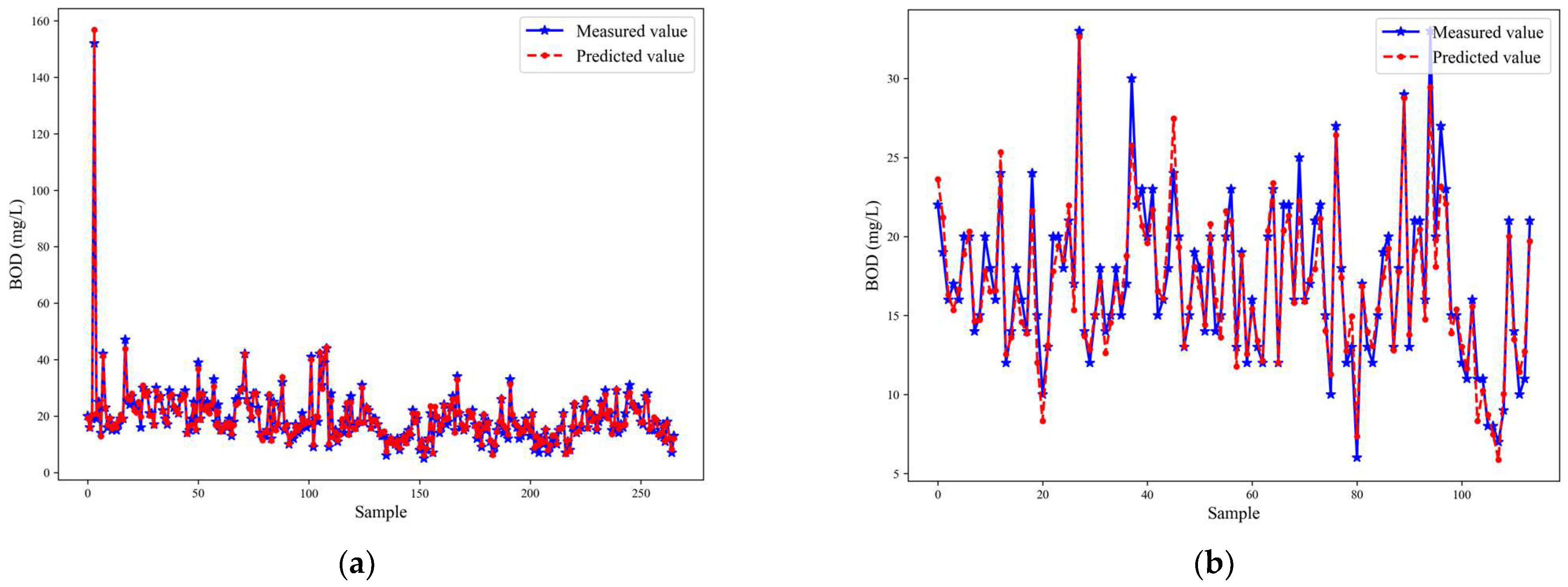
Figure 5a,b display the prediction results of the DMST-Transformer model on the training and test sets, respectively. It is observed that the predicted BOD values closely follow the trend of actual measurements, with no obvious lag or overshooting across the full time horizon. The prediction curve on the test set shows good continuity and stability, indicating the robustness of the model under varying input conditions.
Beyond accuracy, we further assessed the computational efficiency and scalability of the models. As shown in Table 4, the symmetric DMST-Transformer requires 0.66 s for inference on the test set, which is faster than the asymmetric ST-Transformer (0.86 s) and the ablation variant T-SGCN-Transformer (0.92 s), while significantly outperforming them in accuracy. Although it is slower than the lightweight LR model (0.01 s) and GCN (0.21 s), the DMST-Transformer achieves a superior balance between runtime and predictive performance, reinforcing its suitability for real-time wastewater monitoring applications.
Furthermore, the ablation variants of the DMST-Transformer (e.g., without SGCN or DST module) show reduced inference times but also exhibit corresponding drops in prediction accuracy, highlighting the role of each architectural component in balancing efficiency and performance. Due to its parallelizable dual-pathway design and modular integration, the symmetric architecture also scales more effectively with increasing feature dimensions and sequence lengths. These findings reinforce the suitability of the DMST-Transformer for real-time and large-scale deployment in wastewater monitoring systems.
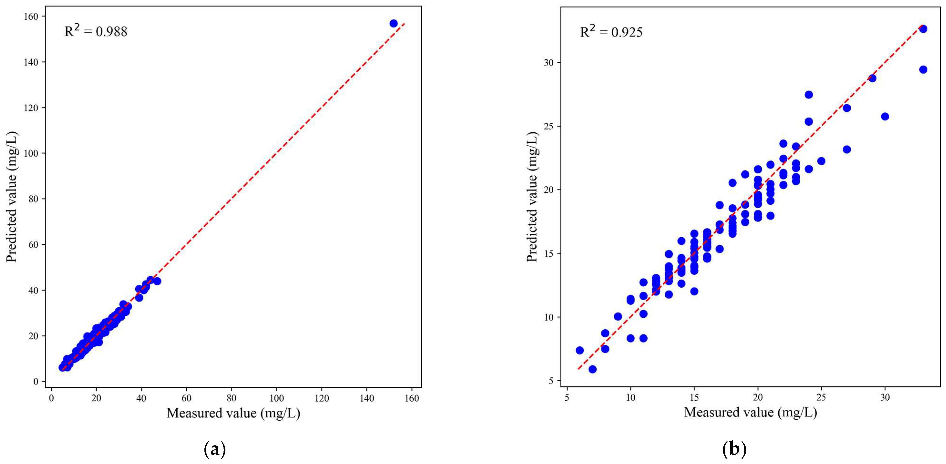
To further evaluate the prediction consistency, Figure 6a,b present scatter plots of predicted values and true values for both training and test sets. The data points align well with the diagonal reference line, especially on the test set, confirming that the model exhibits high accuracy without significant underestimation or overestimation.
To further evaluate the training dynamics and error distribution characteristics of the Benchmark model (ST-Transformer) and the proposed model (DMST-Transformer), Figure 7 and Figure 8 present the training-validation loss curves and residual plots for the ST-Transformer and DMST-Transformer, respectively. As shown in Figure 7a, the ST-Transformer exhibits relatively unstable validation loss with noticeable fluctuations, and early stopping is triggered around the ninetieth epoch. In contrast, the DMST-Transformer shown in Figure 7b converges faster and more smoothly, with early stopping occurring at approximately the fiftieth epoch. This indicates a more efficient and stable training process.
Further assessing the prediction performance, Figure 8 shows the residual plots of predicted BOD values. It can be observed that the ST-Transformer displays a wider spread and more extreme residuals, particularly in the high-value prediction range. In comparison, the DMST-Transformer shows more compact and symmetric residuals around zero, suggesting better predictive stability and error control under varying input conditions. These results support the observed improvements in MAPE and RMSE, confirming that the proposed DMST-Transformer model not only enhances prediction accuracy but also improves practical applicability for robust and stable effluent quality monitoring in wastewater treatment systems.
Figure 9 presents the SHAP summary plot of the DMST-Transformer model, illustrating the distribution of feature contributions to the predicted effluent BOD across all samples. Each dot represents the SHAP value of a particular feature for one observation, with color indicating the original feature value (red for high, blue for low). The features are ranked by their average SHAP value, with influent BOD (BOD-E, SHAP = 3.39), primary settler conductivity (COND-P, SHAP = 2.54), and influent flow rate (Q-E, SHAP = 2.48) emerging as the most influential variables. BOD-E not only holds the highest average SHAP score but also consistently exhibits a positive contribution to the predicted output when its value is high, confirming its pivotal role in determining effluent quality. Conversely, variables such as suspended solids and sediment concentrations in the primary settler (e.g., SS-P, SED-P) show relatively low and stable SHAP values, indicating limited predictive relevance in this context. Further analysis of feature importance aggregated by treatment stage reveals that the influent stage alone accounts for 45.6% of the total contribution, underscoring the engineering principle of source control in wastewater management. These results provide strong support for the inclusion of spatial modeling components in the symmetric architecture and offer practical guidance for optimizing sensor placement and process control strategies based on data-driven insights.
In summary, the comparative analysis confirms that architectural symmetry plays a critical role in enhancing spatio-temporal modeling performance for wastewater quality prediction. The proposed DMST-Transformer consistently achieved the best results across all evaluation metrics while maintaining reasonable computational efficiency (inference time 0.66 s, lower than most asymmetric variants). This balance between accuracy and efficiency underscores its practical applicability in real-world wastewater treatment scenarios. Furthermore, the ablation results validate that each architectural module (SGCN, MSSA, and DST) contributes distinct and complementary benefits to the final performance. These findings not only support the theoretical rationale for adopting symmetric designs but also provide actionable insights for future deployment of intelligent monitoring systems in environmental and industrial contexts.

4. Conclusions

This study presents a comparative investigation into symmetric and asymmetric Transformer architectures for spatio-temporal modeling in the context of wastewater treatment. The proposed DMST-Transformer introduces a symmetric design that integrates spatial and temporal modeling through parallel pathways and feature concatenation, in contrast to the sequential addition-based fusion adopted by asymmetric models.
Experimental results demonstrate that the DMST-Transformer consistently achieves superior performance across all evaluation metrics, including a test R2 of 0.93, RMSE of 1.40 mg/L, and MAPE of 6.61%, significantly outperforming traditional models such as linear regression (R2 = 0.65), PLS (R2 = 0.68), and advanced baselines like GCN (R2 = 0.51) and ST-Transformer (R2 = 0.77). These findings validate the effectiveness of architectural symmetry in preserving both spatial and temporal feature integrity, leading to improved predictive accuracy and robustness under dynamic operating conditions.
Beyond accuracy, the DMST-Transformer also demonstrates competitive computational efficiency, with an inference time comparable to or lower than that of several asymmetric variants, reinforcing its suitability for real-time deployment in wastewater monitoring systems. The ablation analysis further confirms the complementary roles of the SGCN, MSSA, and DST modules, providing empirical justification for each architectural component.
Despite its advantages, the study has limitations. The dataset is relatively small and originates from a single wastewater treatment plant, which may affect the model’s generalizability to other facilities or broader water quality indicators. Furthermore, the limited sample size increases the potential risk of overfitting, despite the use of dropout regularization and early stopping. In addition, although the model demonstrates promising real-time prediction potential, it has not yet been deployed in an actual operational environment.
Future work will focus on validating the model across multiple datasets and treatment plants to assess its transferability and robustness. We also plan to extend the model to multi-target prediction tasks (e.g., COD, SS, pH), explore adaptive deployment strategies, and integrate the model into real-time monitoring platforms for continuous effluent quality management. These efforts aim to bridge the gap between academic research and industrial application in the field of intelligent environmental monitoring.

Author Contributions

Conceptualization, T.H. and H.L.; methodology, T.H. and H.L.; software, T.H.; validation, T.H., Z.C. and J.S.; data curation, Z.C.; writing—original draft preparation, T.H.; writing—review and editing, H.L.; supervision, H.L. All authors have read and agreed to the published version of the manuscript.

Funding

This work was supported by the Postgraduate Research & Practice Innovation Program of Jiangsu Province, China (SJCX24_0400), Shandong Provincial Natural Science Foundation, China (ZR2021MF135), and Natural Science Foundation of Jiangsu Provincial Universities, China (22KJA530003).

Data Availability Statement

The data presented in this study are openly available in the Water Treatment Plant—UCI Machine Learning Repository at 10.24432/C5FS4C, reference number 106.

Conflicts of Interest

The authors declare no conflicts of interest.

References

  1. Hu, G.; Li, J.; Zeng, G. Recent development in the treatment of oily sludge from petroleum industry: A review. J. Hazard. Mater. 2013, 261, 470–490. [Google Scholar] [CrossRef]
  2. Li, J.; Du, Q.; Peng, H.; Zhang, Y.; Bi, Y.; Shi, Y.; Xu, Y.; Liu, T. Optimization of biochemical oxygen demand to total nitrogen ratio for treating landfill leachate in a single-stage partial nitrification-denitrification system. J. Clean. Prod. 2020, 266, 121809. [Google Scholar] [CrossRef]
  3. Ma, J.; Ding, Y.; Cheng, J.C.P.; Jiang, F.; Xu, Z. Soft detection of 5-day BOD with sparse matrix in city harbor water using deep learning techniques. Water Res. 2020, 170, 115350. [Google Scholar] [CrossRef] [PubMed]
  4. Song, P.; Huang, G.; An, C.; Shen, J.; Zhang, P.; Chen, X.; Shen, J.; Yao, Y.; Zheng, R.; Sun, C. Treatment of rural domestic wastewater using multi-soil-layering systems: Performance evaluation, factorial analysis and numerical modeling. Sci. Total Environ. 2018, 644, 536–546. [Google Scholar] [CrossRef] [PubMed]
  5. Solgi, A.; Pourhaghi, A.; Bahmani, R.; Zarei, H. Improving SVR and ANFIS performance using wavelet transform and PCA algorithm for modeling and predicting biochemical oxygen demand (BOD). Ecohydrol. Hydrobiol. 2017, 17, 164–175. [Google Scholar] [CrossRef]
  6. Del Rio-Chanona, E.A.; Cong, X.; Bradford, E.; Zhang, D.; Jing, K. Review of advanced physical and data-driven models for dynamic bioprocess simulation: Case study of algae–Bacteria consortium wastewater treatment. Biotechnol. Bioeng. 2019, 116, 342–353. [Google Scholar] [CrossRef]
  7. Huang, R.; Ma, C.; Ma, J.; Huangfu, X.; He, Q. Machine learning in natural and engineered water systems. Water Res. 2021, 205, 117666. [Google Scholar] [CrossRef]
  8. Zaghloul, M.S.; Hamza, R.A.; Iorhemen, O.T.; Tay, J.H. Comparison of adaptive neuro-fuzzy inference systems (ANFIS) and support vector regression (SVR) for data-driven modelling of aerobic granular sludge reactors. J. Environ. Chem. Eng. 2020, 8, 103742. [Google Scholar] [CrossRef]
  9. Yu, H.; Song, Y.; Liu, R.; Pan, H.; Xiang, L.; Qian, F. Identifying changes in dissolved organic matter content and characteristics by fluorescence spectroscopy coupled with self-organizing map and classification and regression tree analysis during wastewater treatment. Chemosphere 2014, 113, 79–86. [Google Scholar] [CrossRef]
  10. Harrou, F.; Cheng, T.; Sun, Y.; Leiknes, T.; Ghaffour, N. A Data-Driven Soft Sensor to Forecast Energy Consumption in Wastewater Treatment Plants: A Case Study. IEEE Sens. J. 2021, 21, 4908–4917. [Google Scholar] [CrossRef]
  11. Li, Z.; Ma, X.; Xin, H. Feature engineering of machine-learning chemisorption models for catalyst design. Catal. Today 2017, 280, 232–238. [Google Scholar] [CrossRef]
  12. Dittrich, I.; Gertz, M.; Maassen-Francke, B.; Krudewig, K.H.; Junge, W.; Krieter, J. Combining multivariate cumulative sum control charts with principal component analysis and partial least squares model to detect sickness behaviour in dairy cattle. Comput. Electron. Agric. 2021, 186, 106209. [Google Scholar] [CrossRef]
  13. Liu, H.; Yang, J.; Zhang, Y.; Yang, C. Monitoring of wastewater treatment processes using dynamic concurrent kernel partial least squares. Process Saf. Environ. Prot. 2021, 147, 274–282. [Google Scholar] [CrossRef]
  14. Alvi, M.; Batstone, D.; Mbamba, C.K.; Keymer, P.; French, T.; Ward, A.; Dwyer, J.; Cardell-Oliver, R. Deep learning in wastewater treatment: A critical review. Water Res. 2023, 245, 120518. [Google Scholar] [CrossRef] [PubMed]
  15. Dong, S.; Wang, P.; Abbas, K. A survey on deep learning and its applications. Comput. Sci. Rev. 2021, 40, 100379. [Google Scholar] [CrossRef]
  16. Pouyanfar, S.; Sadiq, S.; Yan, Y.; Tian, H.; Tao, Y.; Reyes, M.P.; Shyu, M.-L.; Chen, S.-C.; Iyengar, S.S. A Survey on Deep Learning: Algorithms, Techniques, and Applications. ACM Comput. Surv. 2018, 51, 1–36. [Google Scholar] [CrossRef]
  17. Li, X.; Yi, X.; Liu, Z.; Liu, H.; Chen, T.; Niu, G.; Yan, B.; Chen, C.; Huang, M.; Ying, G. Application of novel hybrid deep leaning model for cleaner production in a paper industrial wastewater treatment system. J. Clean. Prod. 2021, 294, 126343. [Google Scholar] [CrossRef]
  18. Xie, W.; Wang, J.; Xing, C.; Guo, S.; Guo, M.; Zhu, L. Variational Autoencoder Bidirectional Long and Short-Term Memory Neural Network Soft-Sensor Model Based on Batch Training Strategy. IEEE Trans. Ind. Inform. 2021, 17, 5325–5334. [Google Scholar] [CrossRef]
  19. Chen, H.; Chen, A.; Xu, L.; Xie, H.; Qiao, H.; Lin, Q.; Cai, K. A deep learning CNN architecture applied in smart near-infrared analysis of water pollution for agricultural irrigation resources. Agric. Water Manag. 2020, 240, 106303. [Google Scholar] [CrossRef]
  20. Yu, M.; Huang, Q.; Li, Z. Deep learning for spatiotemporal forecasting in Earth system science: A review. Int. J. Digit. Earth 2024, 17, 2391952. [Google Scholar] [CrossRef]
  21. Vaswani, A.; Shazeer, N.; Parmar, N.; Uszkoreit, J.; Jones, L.; Gomez, A.N.; Kaiser, Ł.; Polosukhin, I. Attention is all you need. In Proceedings of the Advances in Neural Information Processing Systems 30 (NIPS 2017), Long Beach, CA, USA, 4–9 December 2017. [Google Scholar]
  22. Chang, P.; Zhang, S.; Wang, Z. Soft sensor of the key effluent index in the municipal wastewater treatment process based on transformer. IEEE Trans. Ind. Inform. 2023, 20, 4021–4028. [Google Scholar] [CrossRef]
  23. Chen, Y.; Chen, X.; Xu, A.; Sun, Q.; Peng, X. A hybrid CNN-Transformer model for ozone concentration prediction. Air Qual. Atmos. Health 2022, 15, 1533–1546. [Google Scholar] [CrossRef]
  24. Zhang, Z.; Zhang, S. Modeling air quality PM2. 5 forecasting using deep sparse attention-based transformer networks. Int. J. Environ. Sci. Technol. 2023, 20, 13535–13550. [Google Scholar] [CrossRef]
  25. Tang, S.; Li, C.; Zhang, P.; Tang, R. Swinlstm: Improving spatiotemporal prediction accuracy using swin transformer and lstm. In Proceedings of the IEEE/CVF International Conference on Computer Vision, Paris, France, 2–6 October 2023; pp. 13470–13479. [Google Scholar]
  26. Wen, Q.; Zhou, T.; Zhang, C.; Chen, W.; Ma, Z.; Yan, J.; Sun, L. Transformers in time series: A survey. arXiv 2022, arXiv:2202.07125. [Google Scholar]
  27. Rahali, A.; Akhloufi, M.A. End-to-end transformer-based models in textual-based NLP. AI 2023, 4, 54–110. [Google Scholar] [CrossRef]
  28. Yu, M.; Masrur, A.; Blaszczak-Boxe, C. Predicting hourly PM2. 5 concentrations in wildfire-prone areas using a SpatioTemporal Transformer model. Sci. Total Environ. 2023, 860, 160446. [Google Scholar] [CrossRef]
  29. Geng, Y.; Zhang, F.; Liu, H. Multi-scale temporal convolutional networks for effluent cod prediction in industrial wastewater. Appl. Sci. 2024, 14, 5824. [Google Scholar] [CrossRef]
  30. Wang, P.; Wang, K.; Song, Y.; Wang, X. AutoLDT: A lightweight spatio-temporal decoupling transformer framework with AutoML method for time series classification. Sci. Rep. 2024, 14, 29801. [Google Scholar] [CrossRef]
  31. Naghashi, V.; Boukadoum, M.; Diallo, A.B. A multiscale model for multivariate time series forecasting. Sci. Rep. 2025, 15, 1565. [Google Scholar] [CrossRef] [PubMed]
  32. Liu, Y.; Huang, D.; Li, Y. Development of interval soft sensors using enhanced just-in-time learning and inductive confidence predictor. Ind. Eng. Chem. Res. 2012, 51, 3356–3367. [Google Scholar] [CrossRef]
  33. Luo, L.; Bao, S.; Mao, J. Adaptive Selection of Latent Variables for Process Monitoring. Ind. Eng. Chem. Res. 2019, 58, 9075–9086. [Google Scholar] [CrossRef]
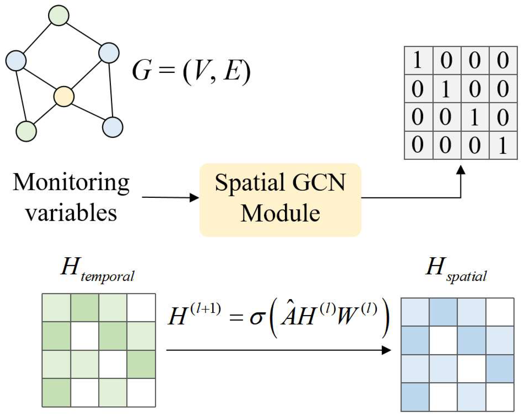
Figure 1. The structure of the SGCN module.
Symmetry 17 01322 g001
Figure 2. The Benchmark Architecture: asymmetric ST-Transformer model.
Symmetry 17 01322 g002
Figure 3. The Proposed Architecture: symmetric DMST-Transformer model.
Symmetry 17 01322 g003
Figure 4. Flowchart of wastewater variables and monitoring locations.
Symmetry 17 01322 g004
Figure 5. The prediction results of the DMST-Transformer model: (a) training set, (b) test set.
Symmetry 17 01322 g005
Figure 6. Scatter plots of measured and predicted values: (a) training set, (b) test set.
Symmetry 17 01322 g006
Figure 7. Training and validation loss curves: (a) ST-Transformer, (b) DMST-Transformer.
Symmetry 17 01322 g007
Figure 8. Residual plots of predicted BOD values: (a) ST-Transformer, (b) DMST-Transformer.
Symmetry 17 01322 g008
Figure 9. SHAP summary plot of the DMST-Transformer model showing feature impacts across all samples.
Symmetry 17 01322 g009
Table 1. WWTP variables used in this work.
PositionVariables
Influent to WWTPFlow (Q-E), Zinc (Zn-E), pH (pH-E), Biological oxygen demand (BOD-E), chemical oxygen demand (COD-E), suspended solids (SS-E), volatile suspended solids (VSS-E), sediments (SED-E), conductivity (COND-E)
Primary settlerspH (pH-P), Biological oxygen demand (BOD-P), suspended solids (SS-P), volatile suspended solids (VSS-P), sediments (SED-P), conductivity (COND-P)
Secondary settlerspH (pH-D), Biological oxygen demand (BOD-D), chemical oxygen demand (COD-D), suspended solids (SS-D), volatile suspended solids (VSS-D), sediments (SED-D), conductivity (COND-D)
Returned sludgeBiological oxygen demand (RD-BOD-P), suspended solids (RD-SS-P), sediments (RD-SED-P)
Wasted sludgeBiological oxygen demand (RD-BOD-S), chemical oxygen demand (RD-COD-S)
Aeration tanksBiological oxygen demand (RD-BOD-G), chemical oxygen demand (RD-COD-G), suspended solids (RD-SS-G), sediments (RD-SED-G)
EffluentpH (pH-S), Biological oxygen demand (BOD-S), chemical oxygen demand (COD-S), suspended solids (SS-S), volatile suspended solids (VSS-S), sediments (SED-S), conductivity (COND-S)
Table 2. Architecture-related hyperparameters of ST-Transformer.
LayerOutput Size
Input[batch, 10, 31]
Temporal Encoding[batch, 10, 64]
Spatial Embedding[batch, 10, 64]
Spatio-Temporal Fusion[batch, 10, 64]
Transformer Block-1[batch, 10, 31]
Multi-Head Attention[batch, 10, 31]
LayerNorm[batch, 10, 31]
Dropout (0.3)[batch, 10, 31]
Feed-Forward[batch, 10, 31]
Transformer Encoder-2[batch, 10, 31]
Average Pooling[batch, 31]
Dense[batch, 1]
Table 3. Architecture-related hyperparameters of DMST-Transformer.
LayerOutput Size
Input[batch, 10, 31]
Positional Encoding[batch, 10, 31]
Adjacency Matrix[31, 31]
GraphConv-1[batch, 10, 64]
GraphConv-2[batch, 10, 31]
Multi-Scale Attention (D = 1)[batch, 10, 31]
Multi-Scale Attention (D = 2)[batch, 10, 31]
Multi-Scale Attention (D = 4)[batch, 10, 31]
Dynamic Self-Tuning (DST)[batch, 10, 31]
Transformer Block-1[batch, 10, 31]
Multi-Head Attention[batch, 10, 31]
LayerNorm[batch, 10, 31]
Dropout (0.1)[batch, 10, 31]
Feed-Forward[batch, 10, 31]
Transformer Block-2[batch, 10, 31]
Average Pooling[batch, 31]
Dense[batch, 1]
Table 4. Comparison of effluent BOD prediction performance using different models.
ModelsBOD
R2RMSE (mg/L)MAPE (%)Times (s)
LRTraining set0.715.8225.120.01
Test set0.652.9715.07
PLSTraining set0.893.5714.090.01
Test set0.683.1113.63
GCNTraining set0.755.4828.740.21
Test set0.514.6624.58
Transformer
(Asymmetric)
Training set0.913.3513.530.5
Test set0.722.7213.22
ST-Transformer
(Asymmetric)
Training set0.942.6711.830.86
Test set0.772.4412.89
DMST-Transformer
(Symmetric)
Training set0.991.195.470.66
Test set0.931.406.61
T-SGCN-Transformer
(Asymmetric)
Training set0.912.5610.350.92
Test set0.852.2910.92
T-MSSA-DST-Transformer
(Asymmetric)
Training set0.892.6310.770.75
Test set0.812.3411.13
T-SGCN-MSSA-Transformer
(Symmetric)
Training set0.951.678.420.68
Test set0.891.728.89
Disclaimer/Publisher’s Note: The statements, opinions and data contained in all publications are solely those of the individual author(s) and contributor(s) and not of MDPI and/or the editor(s). MDPI and/or the editor(s) disclaim responsibility for any injury to people or property resulting from any ideas, methods, instructions or products referred to in the content.