Abstract
Self-Organizing Map (SOM) neural networks can project complex, high-dimensional data onto a two-dimensional plane for data visualization, enabling an intuitive understanding of the distribution and symmetric structures of such data, thereby facilitating the clustering and anomaly detection of complex high-dimensional data. However, this algorithm is sensitive to the initial weight matrix and suffers from insufficient feature extraction. To address these issues, this paper proposes an improved SOM based on virtual winning neurons (virtual-winner SOMs, vwSOMs). In this method, the principal component analysis (PCA) is utilized to generate the initial weight matrix, allowing the weights to better capture the main features of the data and thereby enhance clustering performance. Subsequently, when new input sample data are mapped to the output layer, multiple neurons with a high similarity in the weight matrix are selected to calculate a virtual winning neuron, which is then used to update the weight matrix to comprehensively represent the input data features within a minimal error range, thus improving the algorithm’s robustness. Multiple datasets were used to analyze the clustering performance of vwSOM. On the Iris dataset, the S is 0.5262, the F1 value is 0.93, the ACC value is 0.9412, and the VA is 0.0012, and the experimental result with the Wine dataset shows that the S is 0.5255, the F1 value is 0.93, the ACC value is 0.9401, and the VA is 0.0014. Finally, to further demonstrate the performance of the algorithm, we use the more complex Waveform dataset; the S is 0.5101, the F1 value is 0.88, the ACC value is 0.8931, and the VA is 0.0033. All the experimental results show that the proposed algorithm can significantly improve clustering accuracy and have better stability, and its algorithm complexity can meet the requirements for real-time data processing.
1. Introduction
1.1. Motivation and Incitement
Machine learning (ML) is the process by which a computer automatically learns general rules or knowledge from a limited set of observed samples and then induces and generalizes them to unknown samples [1]. In recent years, ML technology has rapidly advanced and plays a crucial role in fields such as agriculture, industry, economics, and medicine. It is commonly used for natural language processing, image processing, and data analysis. When analyzing data using ML technology, tasks often include clustering analysis, anomaly detection, association rule mining, and predictive modeling.
Anomaly detection refers to the identification of data patterns that are significantly different from the majority of the data, i.e., objects in a dataset that are markedly distinct from other data points [2,3]. One kind of traditional method for data anomaly detection often involves modeling using a statistical distribution and then using this model to determine whether the distribution of a data point is anomalous. The others need set thresholds for single measurements and identify outliers based on these thresholds to detect “dirty data”. However, due to the complexity of real-world data and the fact that it may not necessarily conform to any ideal statistical distribution model, results obtained from traditional anomaly detection methods tend to be one-sided. It is difficult to distinguish the types of anomalies and impossible to make joint judgments.
1.2. A Review of Related Literature
In order to efficiently and accurately detect anomalies and high-quality data mining, researchers have been integrating ML technology with data anomaly detection in recent years to enhance traditional algorithms and address simple problems.
Based on the information provided by the training samples and the different feedback mechanisms, ML techniques used for anomaly detection can be divided into two main categories: supervised learning and unsupervised learning [4,5].
In supervised anomaly detection methods, labeled information is utilized to establish a mapping relationship between the input data and their corresponding labels by constructing a classification or regression model. Different mapping relationships reflect the “normal” and “anomalous” states of the data. Subsequently, the model can determine whether test data are normal or anomalous based on the mapping relationship between the data and their label. Classical algorithms for supervised learning include decision trees (DTs), linear regression, K-Nearest neighbor (KNN), and linear support vector machine (SVM) [6]. When using supervised learning for anomaly detection, leveraging data label information can improve model accuracy. However, issues such as class imbalance may arise when the volume of anomalous data is small. Additionally, the performance of supervised learning algorithms can be compromised when dataset labels are missing, which can impact the detection results.
In real life, due to a lack of prior knowledge, the labels for most datasets are not fully known. It is difficult to manually label all the data, making it impractical to train supervised models. Therefore, the practical application of unsupervised learning is more widespread. Unsupervised learning can analyze and process datasets without labels; that is to say, unsupervised learning algorithms can identify or differentiate data by learning the inherent patterns in the data without any prior knowledge. Common unsupervised algorithms fall into two categories: clustering and dimensionality reduction. Clustering algorithms include k-means clustering, hierarchical clustering, and DBSCAN clustering [7], while dimensionality reduction algorithms include principal component analysis (PCA), singular value decomposition (SVD), and others. When the minority of samples in a dataset are abnormal values that differ significantly from the normal data, unsupervised anomaly detection methods can be used [8]. During the algorithm training process, no labels are needed for correction. Data anomalies are typically reflected in aspects such as the distance between data points, distribution density, and deviation degree. By identifying the feature relationships between data points, the algorithm detects the most dissimilar samples as anomalous test data compared to other data points. The idea of determining outlier points based on clustering is that data points are out of any cluster. Additionally, data points are also considered anomalies when they are far from the cluster center or in clusters with sparse data points. Depending on the specific anomaly patterns, suitable unsupervised learning models can be selected for anomaly detection. S. Gadal [9] proposes combining k-means clustering with sequential minimal optimization (SMO) for anomaly detection. This hybrid algorithm enhances the accuracy of anomaly detection and controls the false alarm probability (FAP) within a low threshold. However, this algorithm only divides the dataset into normal and anomaly classes without further categorization of anomaly data and has high complexity. M. Jain [10] combines k-means clustering with data capture and drift analysis, reducing data volume to enhance the training dataset. However, this algorithm can provide more consistent accuracy and FAP for detecting network traffic anomalies. It has unstable accuracy and F1 values when dealing with datasets with diverse traffic patterns and large capacities. The literature [11] introduces a parameter self-selecting DBSCAN model that improves upon the challenge of parameter selection in traditional DBSCAN. It can effectively cluster multidimensional data with a smaller minimum points (minPts) setting and perform anomaly detection on real-time collected data. Nevertheless, the small minPts parameter may cause over-dispersed clustering, potentially grouping noise data into clusters in practical applications. The literature [12] presents an anomaly detection method based on PCA and isolation forest for analyzing user access data flow on website platforms. While this method enhances the computational efficiency of traditional isolation forest algorithms, it still faces challenges such as low detection accuracy and poor generalization capabilities. Table 1 shows the performance of various clustering algorithms.

Table 1.
Comparison table of the performance of various clustering algorithms.
As a classic clustering model in unsupervised learning, a Self-Organizing Map (SOM) can be used for data visualization, clustering, classification, feature extraction, and other purposes [13,14,15,16]. A SOM reveals the distribution and symmetric structures of complex, high-dimensional data, which are understood through topological mapping and distance-based neighborhood learning mechanisms. Symmetric patterns in high-dimensional spaces typically manifest as geometrically or distributionally equivalent clusters. Detecting symmetric groups enhances clustering validity, while asymmetric deviations—such as neuron weight vectors breaking expected symmetry—can flag potential outliers. This capability significantly facilitates both clustering of high-dimensional data and anomaly detection. Training a SOM network maps input data onto nodes in the output layer, where nodes are arranged based on their distance relationships. This approach allows the network to learn the intrinsic features of the data and understand the topological relationships between different data points. The traditional SOM algorithm is easy to implement and has low computational complexity.
In recent years, many scholars have optimized the traditional SOM algorithm. All these methods have advantages and disadvantages. Z. Sandoval-Lara et al. proposed the Growing Self- Organizing Map algorithm (GSOM) [17], which dynamically increases the number of neurons in the SOM during the training process to adapt to the shape of the data as needed. Compared to traditional fixed-size models, this algorithm exhibits higher robustness on datasets of different sizes. However, it involves a larger number of model learning iterations and does not consider the impact of noise in the data. W. Cui et al. combined SOM with the Support Vector Machine algorithm (SVM) for intermittent fault diagnosis in devices [18]. They introduced a labeling process based on a majority voting strategy before training the SOM network. This process generates a labeled SOM model for identifying data. And then, the SVM algorithm is used to further process the inputs judged as normal or faulty states. By performing two-step anomaly detection, the accuracy of intermittent fault diagnosis is improved. However, labeling the unsupervised SOM model through voting increases the algorithm’s complexity and introduces errors in data labeling judgment. X. Zhang et al. proposed an anomaly detection algorithm that combines SOM with the backpropagation neural network (BP) [19]. This algorithm overcomes the SOM model’s inability to directly judge the correctness of clustering results and the difficulty in understanding clustering results, leading to the improvement of stability and accuracy of the detection results. Unfortunately, it may have error accumulation from the clustering to the classification process when the samples’ differences are not significant. S. Chen et al. proposed to integrate the dimensionality reduction of the Uniform Manifold Approximation and Projection algorithm (UMAP) with the SOM model’s representation of data topological structures [20]. By establishing the global relationships between samples correctly and preserving the internal spatial structures of most category samples as much as possible, the UMAP-SOM achieved more reliable classification. Nevertheless, the UMAP dimensionality reduction algorithm requires multiple experiments to determine the appropriate parameter size. Additionally, it constructs high-dimensional graph representations using local distances, leading to the loss of meaning in cluster sizes and distances between clusters. Table 2 shows that the performance of various SOM algorithms.
Table 2.
Comparison table of the performance of various SOM algorithms.
1.3. Contribution and Paper Organization
The research gap this paper aim to address are as follows.
(1) In the SOM algorithm, the random initialization of the weight matrix can slow down the convergence speed of the SOM network and lead to getting stuck in local optima when exploring the parameter space.
(2) Training the model using a single winning neuron is not conducive to interpreting input data from multiple perspectives and cannot comprehensively represent various aspects of the data’s features.
(3) The sensitivity of the algorithm to changes in a single winning neuron makes it susceptible to noise interference in the input data.
In summary, this paper proposes an improved Self-Organizing Map neural network based on virtual winning neurons (vwSOM). This algorithm can reduce the impact of the initial weight matrix on model training and comprehensively characterize data features. Experimental results demonstrate that the proposed algorithm can improve the stability and accuracy of the clustering results.
The contributions of this paper are as follows:
(1) Initializing the weight matrix using PCA, avoiding issues such as slow convergence speed and getting stuck in local optima caused by random initialization of the weight matrix.
(2) When new input sample data are mapped to the output layer, several neurons with high similarity in the weight matrix are selected. Subsequently, a virtual winning neuron is computed to update the weight matrix.
The structure of the paper is as follows: Section 1 includes the significance of the research, the current state of domestic and international research, and the algorithmic contributions of this paper; Section 2 introduces the principles and training process of SOM, providing the technical foundation for the optimization algorithm in the later sections; Section 3 focuses on the proposed vwSOM algorithm, providing a detailed explanation in three parts: PCA initialization of the weight matrix, the principle of virtual winning neurons, and the algorithm process; Section 4 presents the experimental section, where vwSOM is applied to multiple datasets and compared with other algorithms under the same parameter conditions, and the experimental data are explained and analyzed; Section 5 summarizes the advantages of the proposed algorithm and outlines possible directions for future improvement.
2. Related Technology
Principles of SOM
When projecting high-dimensional data onto SOM networks, the intrinsic relationships in the data space are preserved through the following mechanisms:
(1) Neighborhood Preservation: Ensuring that topologically adjacent neurons represent related data points.
(2) Weight Vector Alignment: Adjusting neuron weights to align with symmetry axes in the feature space.
(3) Unified Distance Matrix (U-Matrix): Highlighting symmetric regions through the visualization of inter-neuron distances.
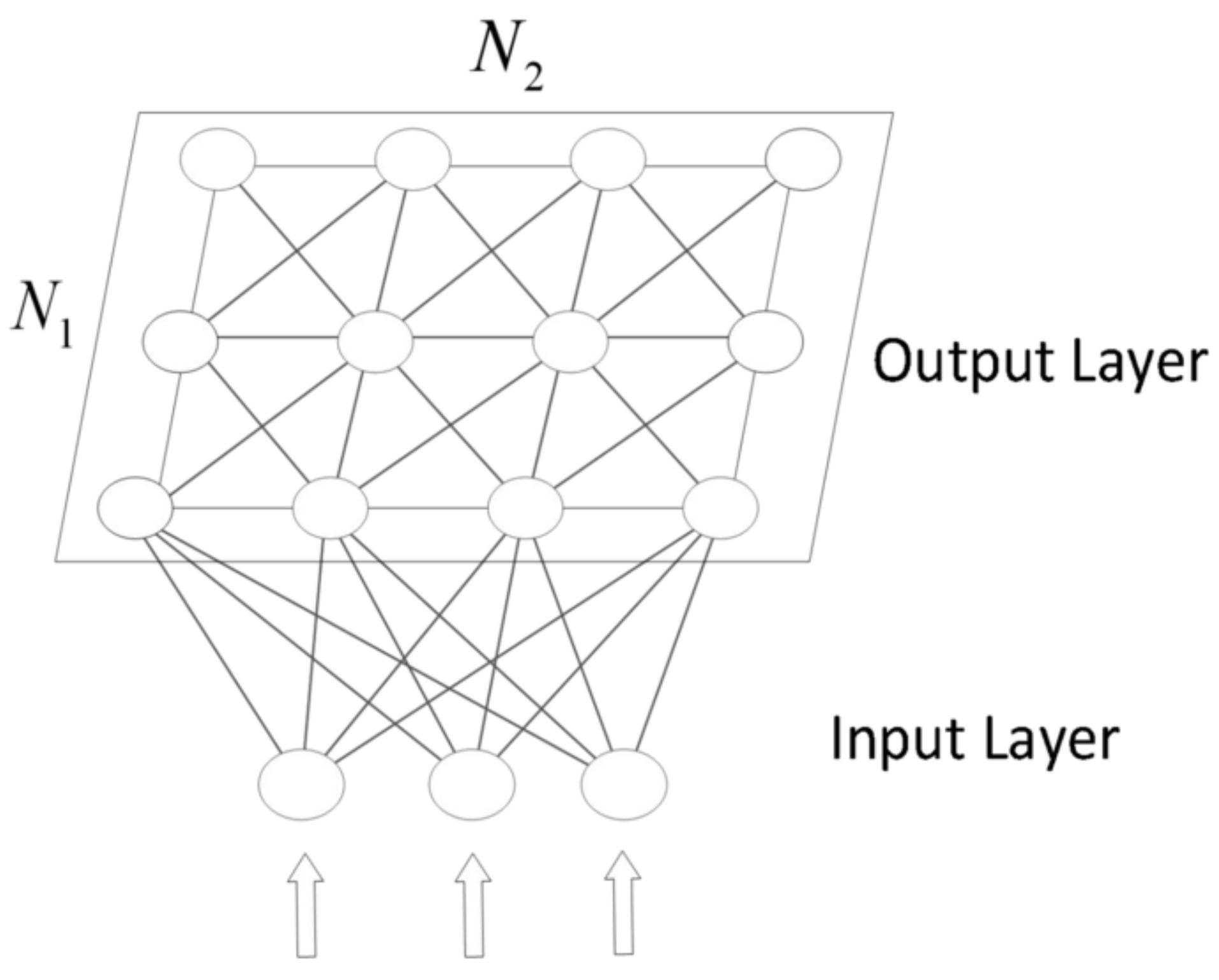
The SOM algorithm consists of two layers: the input layer and the output layer. Its structure is shown in Figure 1. The input layer consists of D nodes, which is the same as the input feature dimensions. The output layer contains · neural nodes, forming a two-dimensional matrix. The input nodes are fully connected to the output layer neurons, and the connecting lines represent the weights. Each neuron in the output layer is represented by a D-dimensional vector . After training, there are certain associations between the nodes of the output layer based on their distances. By learning a set of weights, the input data can be mapped to the output layer nodes. The output layer nodes represent the characteristics of the input data and preserve the topological structure between the input data. This allows for associated data in the input space to cluster together in the output space, forming a set of neurons with correlations. Through multiple iterations, a clustering region will form near each neuron, and the neuron’s weight values in the clustering region will be consistent with or approach the input data. As a result, input data with similar characteristics will be concentrated on adjacent neurons, thus achieving clustering.
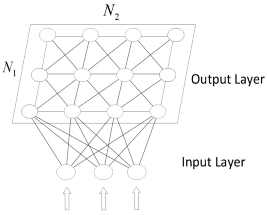
Figure 1.
The architecture of the SOM.
The training process is as follows:
(1) Preprocess the training data. Assume that the size of the training data is N·D, where N is the number of training samples and D is the input feature dimension. Preprocessing the training data includes normalization and regularization. Normalizing the data when the feature values have different ranges ensures that the features have the same measurement scale, which helps improve algorithm accuracy. Regularizing the data prevents overfitting, controls algorithm complexity, and enhances algorithm generalization capability.
(2) Determine the size of the output layer. The performance of the SOM algorithm improves as the number of output layer neurons increases. However, the computational cost will also increase accordingly. Therefore, the size of the output layer can be determined based on the following empirical formula:
(3) Initialize the weight matrix W, with a size of ··D. The weight matrix can be randomly initialized and then regularized.
(4) Iterative training.
Obtain a sample x of training data and calculate the Euclidean distance between x and each node,
Find the closest point as the winning point, i.e., the activated neuron for x. Set the weight of that point to 1. Calculate the weights of other nodes based on the distance between the winning point and themselves in the output layer, leading to the neighborhood function corresponding to this iteration.
Where represents each output layer neuron and is the neighborhood decay rate, which decreases as the number of iterations increases.
Where is the initial neighborhood decay rate, t is the current iteration number, and is the maximum number of iterations.
Update the weight matrix,
This process is similar to finding cluster centers, where each update makes closer to x. Here, is the learning rate, which decreases as the number of iterations increases, so that with each iteration, the weight matrix updates become smaller,
Where is the initial learning rate. The feedback from neurons to input data follows a “Sombrero” function, as shown in Figure 2. The neurons around the winning neuron are in an excited state, while neurons farther away from the winning neuron are in an inhibited state.
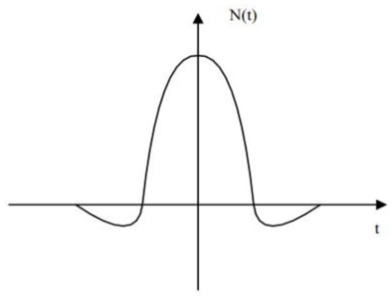
Figure 2.
“Sombrero” function illustration.
After multiple iterations, terminate the iteration when the weight vectors of neurons reach global convergence,
Here, is the mean of all input data mapped to neuron . When the training times are sufficiently large, the weight of each neuron on the output layer becomes infinitely similar to the mean of the input data mapped to it. Therefore, each neuron can be used to represent features of the input data.
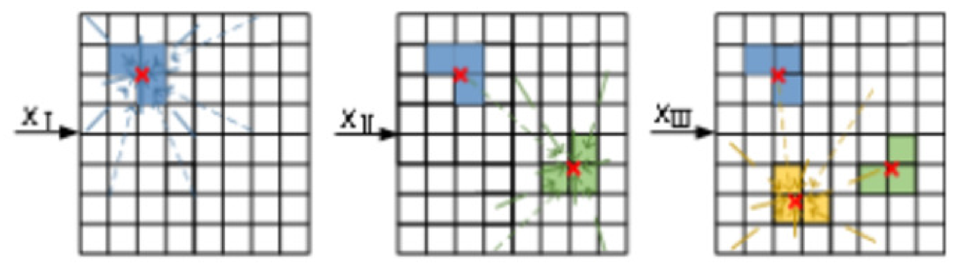
Assume the training data are divided into three categories. During the SOM model training process, the trend of the weight vector changes for each neuron node is shown in Figure 3.
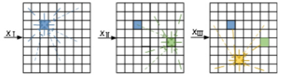
Figure 3.
Diagram of the update of the weight vector in the SOM.
In this figure, , , represent training data from different categories; different colored blocks represent the winning neurons of input data; the thickness and style of the lines indicate the weight vector update rules as shown in Equations (3) and (5), i.e., neurons closer to the winning neuron undergo greater weight vector updates. From the figure, it can be observed that the change in a single winning neuron causes the algorithm to be more sensitive to the input data, making it prone to noise interference. Therefore, this paper proposes the vwSOM model to improve the algorithm’s stability and achieve better clustering results.
3. Principles of vwSOM
3.1. Initialize the Weight Matrix Using the PCA Algorithm
Perform PCA [21] on the preprocessed data to calculate the feature vectors in the dataset, which represent the directions with the maximum variance in the dataset.
Assume the training data matrix:
where each x is a D -dimensional column vector that represents input sample.
Calculate the covariance matrix S:
Perform eigen-decomposition on the covariance matrix S:
Obtain the eigenvalues and their corresponding eigenvectors, arrange them in descending order, and form a matrix P consisting of the eigenvectors corresponding to non-zero eigenvalues, resulting in
where is a diagonal matrix containing the decreasing non-negative real eigenvalues . The eigenvectors corresponding to the largest k eigenvalues as the principal components are chosen, where k is the dimension after dimension reduction. The new data matrix T after PCA with k-dimensional can be obtained,
The extracted principal components are used to initialize the weight matrix of the SOM model, using each principal component as an initial weight vector.
By using PCA to initialize the weight matrix, it provides a good initial state for the subsequent model training, reducing the impact of the initial weight matrix on the clustering algorithm’s effectiveness. This approach helps accelerate the convergence process of the algorithm, reducing training time and computational resource consumption.
3.2. The Virtual Winning Neuron
In the SOM algorithm, the way to update the weight matrix is based on the relationship between the distances of the winning neuron and the other nodes in the output layer after mapping the sample data. By observing the Euclidean distance array between the input samples and the points in the output layer, it is found that the Euclidean distance of the winning neuron node is very similar to that of the surrounding two neurons. This indicates that these three neurons represent the input sample similarly. Inspired by virtual nodes, the SOM algorithm is improved by selecting the three nodes closest to the input sample as the winning neurons. By calculating the distance weights of these three neurons, the weighted average Euclidean distance between the input sample and the three neuron nodes is obtained. The point with the difference from the feature value of x is set as a virtual winning neuron s. The weights of other nodes are updated based on the distance relationship with this virtual node. By changing the number of winning neurons, it is hoped to capture more information under small errors, comprehensively represent the features of input data, and improve the clustering accuracy of the algorithm. In addition, compared to the concept of the single winning neuron, the multi-winning neuron algorithm has lower sensitivity to input data and stronger algorithm stability.
Select the three winning neurons closest to the input sample in terms of Euclidean distance and calculate the distances between the current neuron and these three winning neurons, denoted as . Use an exponential decay rate to calculate the weights of these three distances so that relatively distant winning neurons contribute less to the final weighted distance while relatively close winning neurons contribute more. The decay rate can be controlled by adjusting the parameters in the exponential decay rate. For example:
Based on the distance weights obtained above, calculate the weighted average of the Euclidean distances corresponding to the three winning neurons to obtain the distance between the virtual neuron node s and the current node,
Traverse each neuron in the output layer and update its weight vector ,
where is the neighborhood decay rate, which is shown in Formula (4). And represents the distance between the input sample x and the neuron node at position in the output layer, which is shown in Formula (2).
Assume the training data are divided into three categories. During the training process of the vwSOM model, the trend of the weight vector changes for each neuron node is shown in Figure 4. In this figure, , , represent training data from different categories; different colored blocks represent the winning neurons of input data; the thickness and style of the lines indicate the weight vector update rules; the three same-colored blocks represent the three winning neurons corresponding to the training data; and the red markers represent the virtual winning neuron obtained from Equations (16) and (17). Comparing with Figure 3, it is found that the vwSOM model selects multiple winning neurons for the input data. This method increases the amount of information the model obtains from the input data and allows for a more comprehensive representation of the data characteristics. By calculating the virtual winning neurons and using them for weight updates, the sensitivity of the model to noise interference can be reduced, thereby improving the algorithm’s stability.

Figure 4.
Diagram of virtual winning neurons used to update weight vectors.
3.3. The vwSOM Algorithm
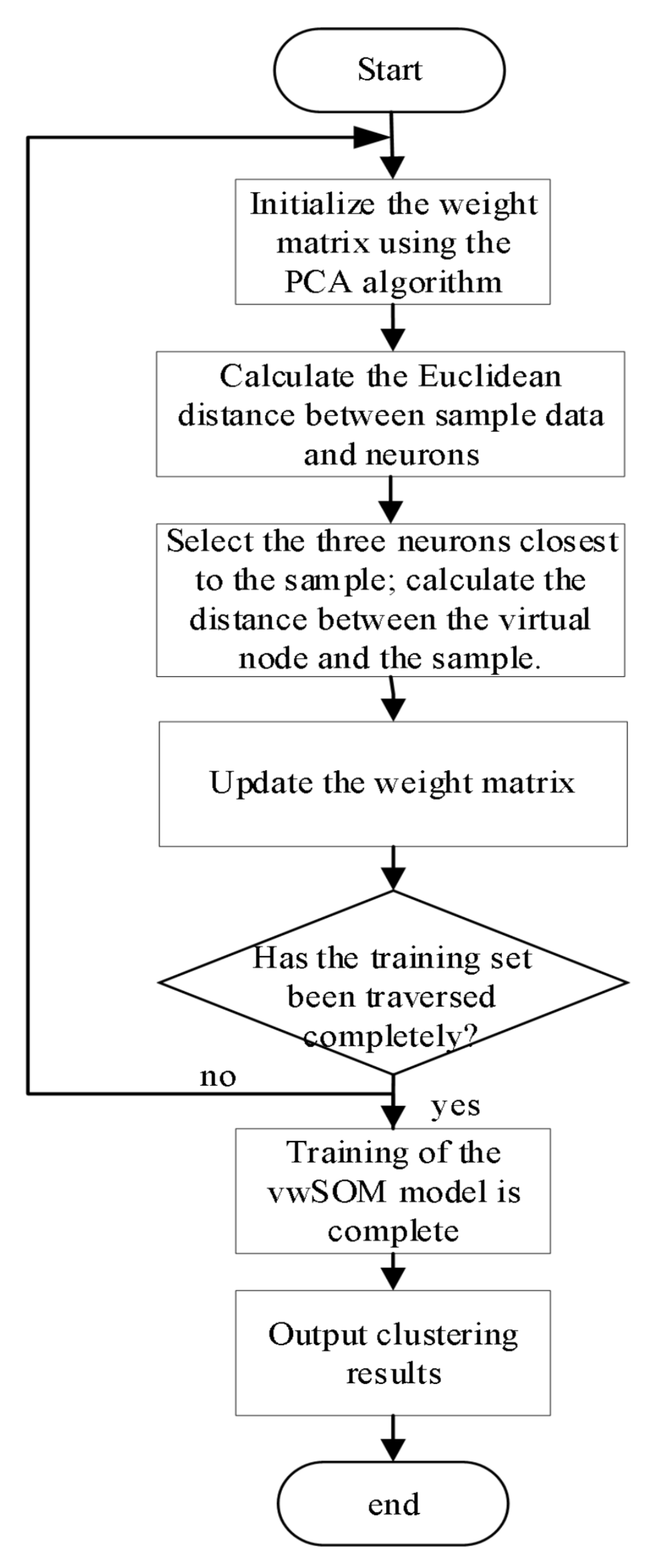
Combining the PCA algorithm with the concept of virtual winning neurons applied to the SOM algorithm, the specific steps are as follows:
(1) Preprocess the training set data and initialize the weight matrix using the PCA algorithm. Select the corresponding feature vectors as initial weight vectors based on the desired number of principal components. The weight matrix constructed in this way is used for subsequent model training.
(2) Iterate through the sample data, calculate the Euclidean distance between the sample and each neuron node, which is calculated as the Euclidean distance between the sample features and each weight vector.
(3) Select the top three neurons with the smallest distances as the winning neurons. Calculate the weighted average of the distances among these three neurons and use the resulting value as the distance between the sample data and the virtual neuron node mapped to the output layer.
(4) Update the weight vectors based on the distance relationship between the virtual neuron node and the other nodes. After iterating through the training set data, the weight matrix is updated.
(5) Iteratively train the model multiple times to make the weight matrix closely approximate the features of the sample data.

Figure 5.
Flowchart of the vwSOM Algorithm.
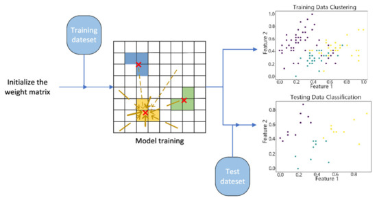
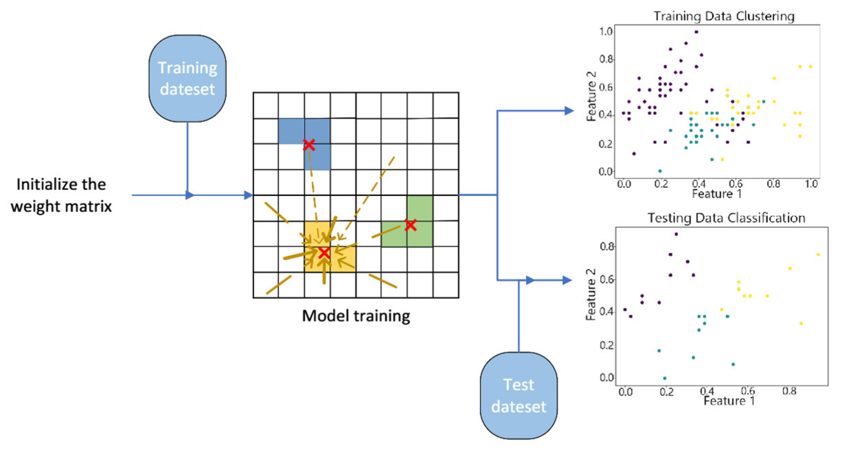
Figure 6.
Structure of the vwSOM Algorithm.
4. Experimental Results and Analysis
4.1. Experimental Setup
Conducting experiments using Python 3.8, we imported the Iris dataset [22] and the Wine dataset [23]. Meanwhile, to further evaluate the algorithm’s performance, we selected the more complex Waveform dataset [24]. Table 3 shows the parameters of the datasets. Each dataset is split into training and testing datasets at a 7:3 ratio. The IRIS dataset is a classic multi-class dataset containing 150 samples, divided into three classes of iris flowers (Setosa, Versicolor, and Virginica). Each sample has four features: sepal length, sepal width, petal length, and petal width. It is commonly used in machine learning and data mining for studying classification algorithms. The Wine dataset contains 178 samples, divided into three classes of different types of wine, with each class containing 59 to 71 samples. Each sample has 13 features, mainly describing the chemical composition of the wine, such as alcohol content, malic acid, and ash. It is commonly used for studying the performance of classification and regression algorithms. The Waveform DataSet contains 5000 samples, each with 21 features representing signals from three different waveform types. The task of the dataset is to identify the signals based on these features. It is commonly used to test the classification and clustering performance of machine learning models. Then Table 4 shows all the hyperparameters used in the experiment.
Table 3.
The parameters of the datasets.
Table 4.
The hyperparameters and optimization methods used during the vwSOM model training.
We compared the vwSOM algorithm with the DBSCAN algorithm, the Hybrid SOM algorithm proposed by Khan et al. [25], and the Dynamic Programming SOM proposed by M. N. Manikant [26]. We used a scatter plot to visualize clustering results. This helps to observe the clustering relationships between different sample data points. It also allows the assessment of the clustering effectiveness of each algorithm. We also analyzed the algorithm performance based on various external evaluation metrics. Finally, we conducted ablation experiments to observe the roles played by different modules in the vwSOM algorithm in terms of accuracy and stability. The parameters in the comparison algorithm are set according to the standards specified in the original text. Hyperparameter tuning was performed consistently across all comparative methods to ensure a fair evaluation.
The true labels of the Iris and the Wine dataset are introduced to calculate various performance metrics such as Accuracy (ACC), Precision (P), Recall (R), and F1 for evaluating the algorithms. ACC represents the proportion of all correctly predicted samples to the total number of samples, measuring the overall prediction accuracy of the model. In the case of imbalanced sample classes, high accuracy may lose its significance. P refers to the ratio of the number of correctly predicted positive class samples to the total number of samples predicted as the positive class, measuring how many of the predicted positive class samples are truly positive. A higher precision indicates a lower misjudgment rate of the model. R represents the ratio of the number of correctly predicted positive class samples to the actual number of positive class samples, measuring the model’s ability to identify positive class samples. A higher recall indicates a higher proportion of correctly identified positive class samples by the model. Precision and recall are often contradictory; improving one may lead to a decrease in the other. Therefore, the F1 score is introduced to measure the model’s performance. F1 is the weighted harmonic mean of precision and recall, comprehensively considering both precision and recall. The silhouette score is calculated by computing the average distance (a) between a sample and other data points within the same cluster, as well as the distance (b) between the sample and the data points in the nearest neighboring cluster. It measures the cohesion and similarity between the sample’s own cluster and the neighboring clusters. The value of the silhouette score ranges from [−1, 1]. A higher silhouette score indicates better compactness within clusters and greater distinction between clusters, suggesting better model performance. The calculation formula is as follows:
where N is the number of clusters. The formulas for calculating the above evaluation metrics are as follows:
As the ACC measures the overall prediction accuracy of the model, we conducted 1000 repeated experiments under the same conditions to calculate the variance of ACC (VA). This variance is used to assess the stability of the algorithm’s clustering effect on the data. The Average Operation Time (AOT) refers to the average time taken by the model to process each test data and is used to measure the algorithm’s complexity.
4.2. Visualization of Clustering Results
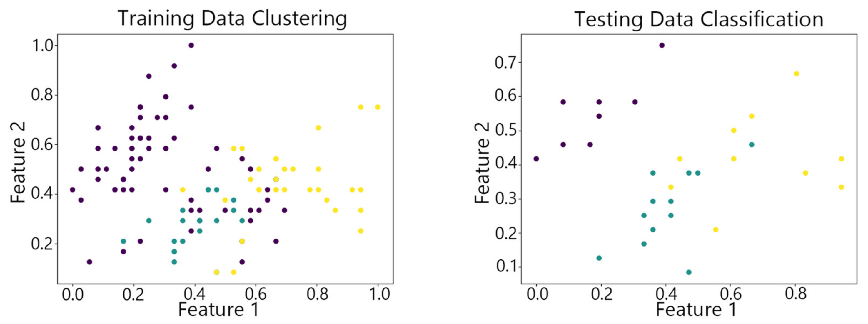
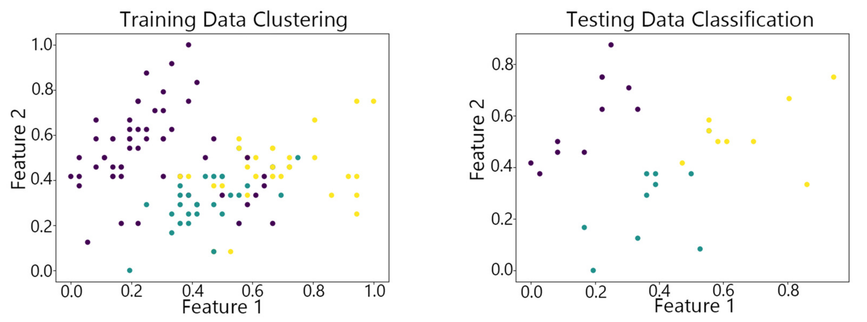
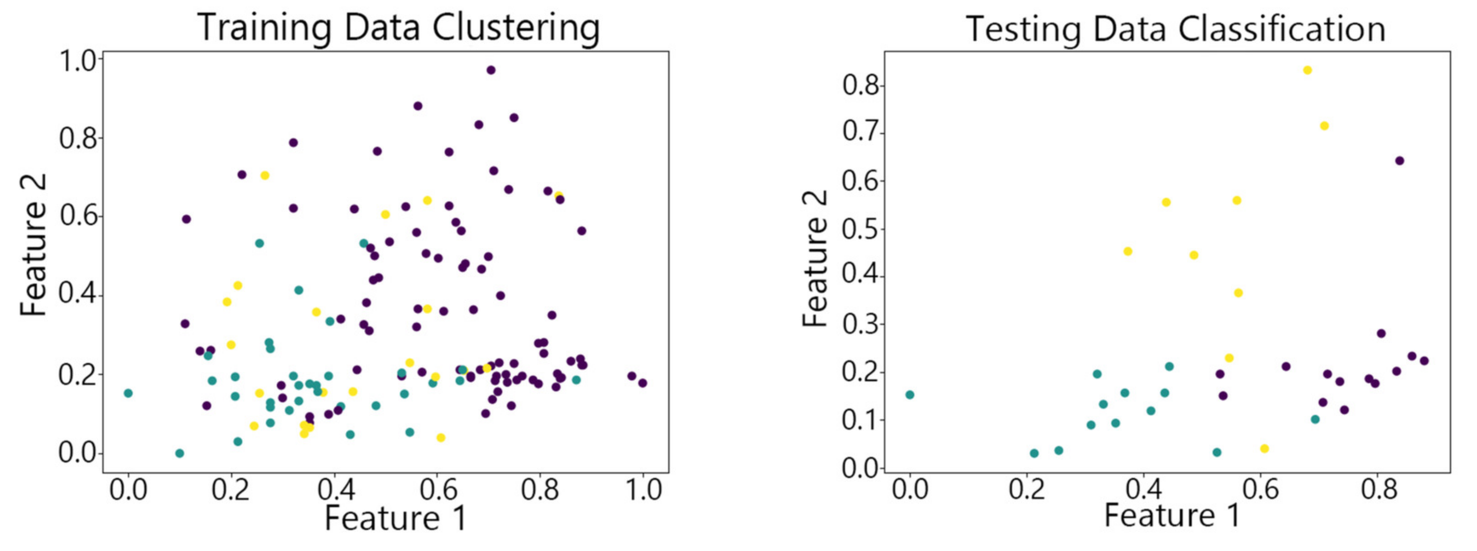
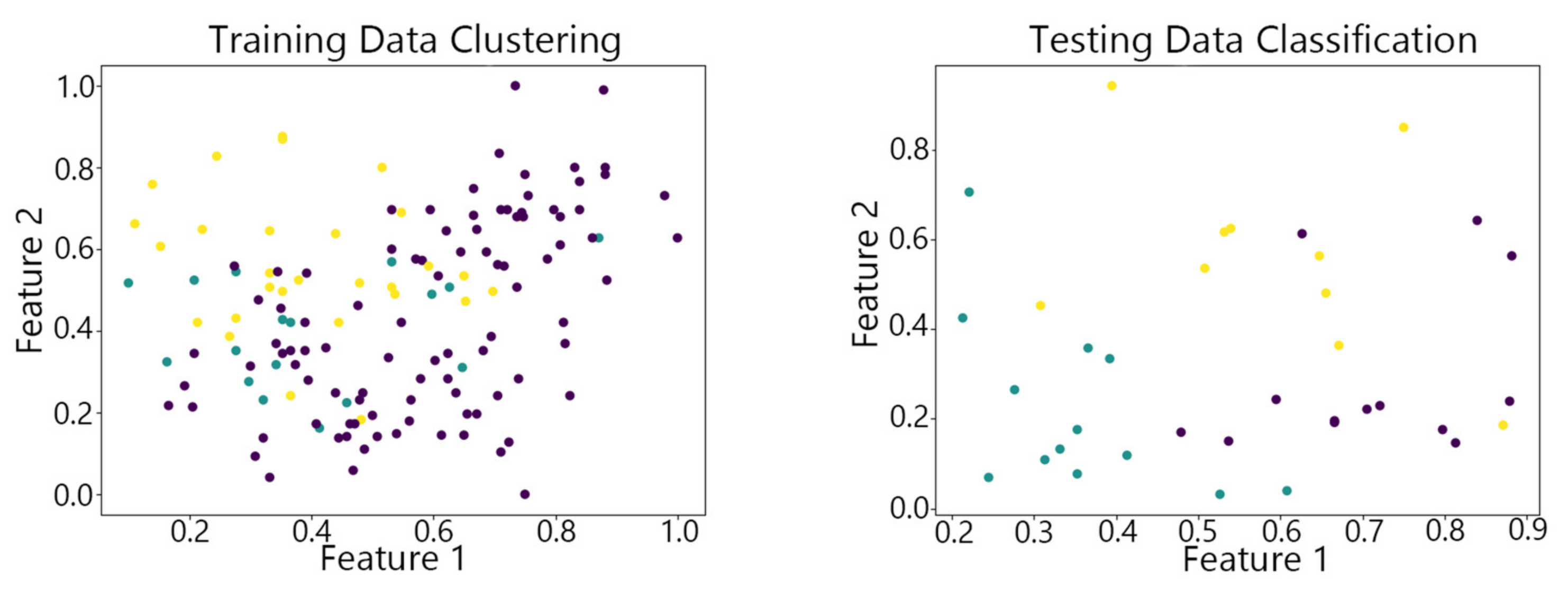
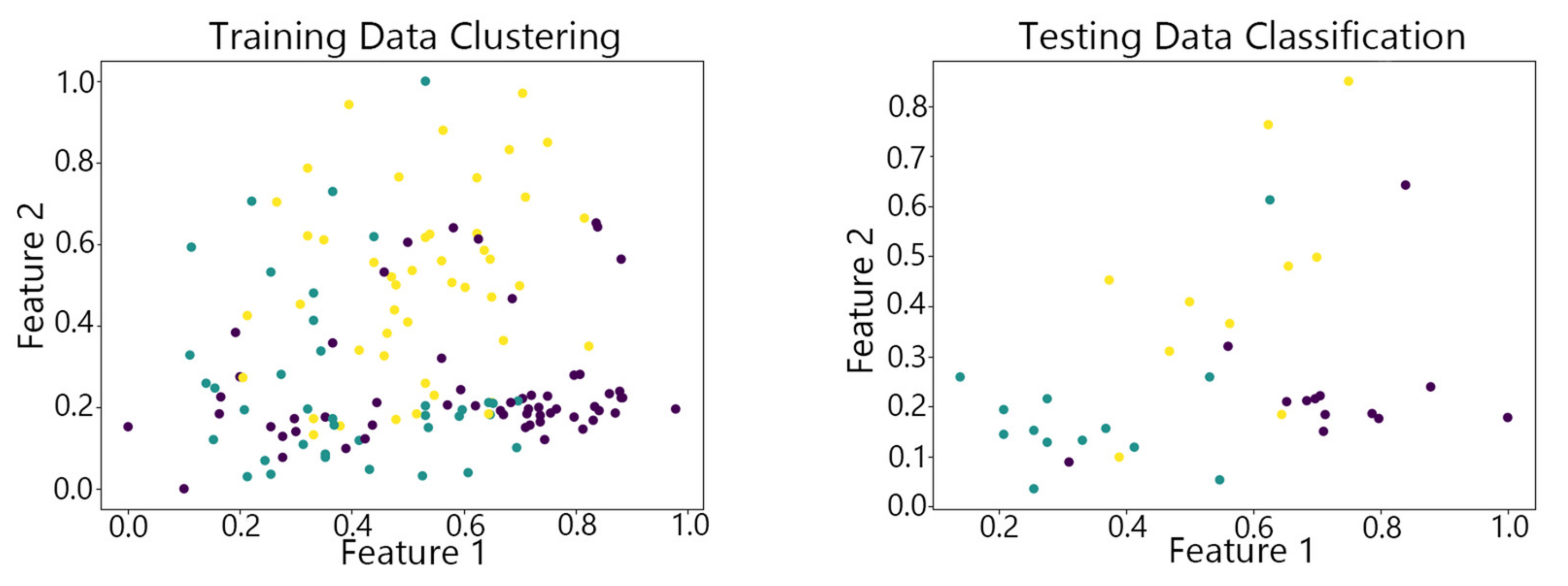
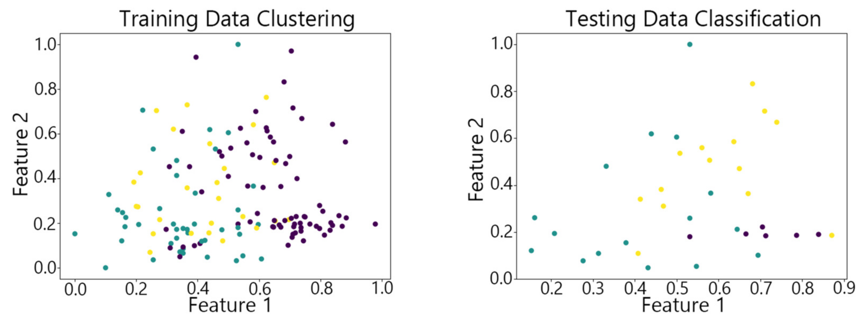
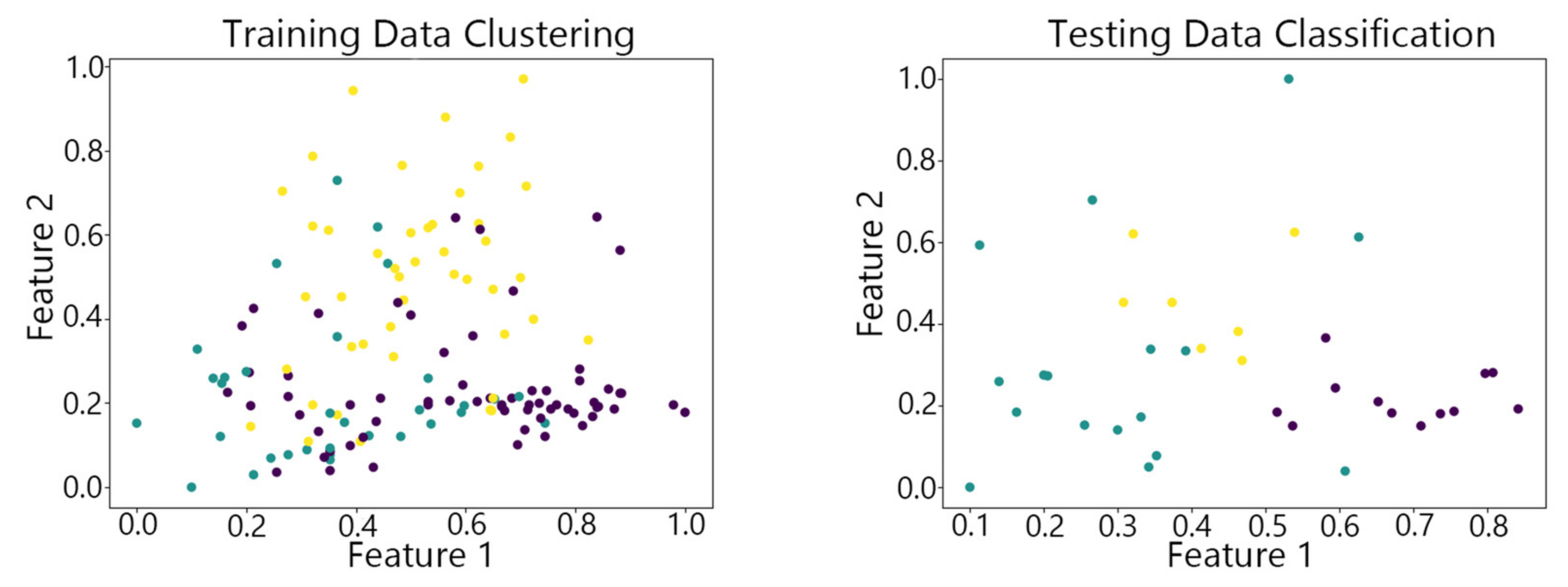
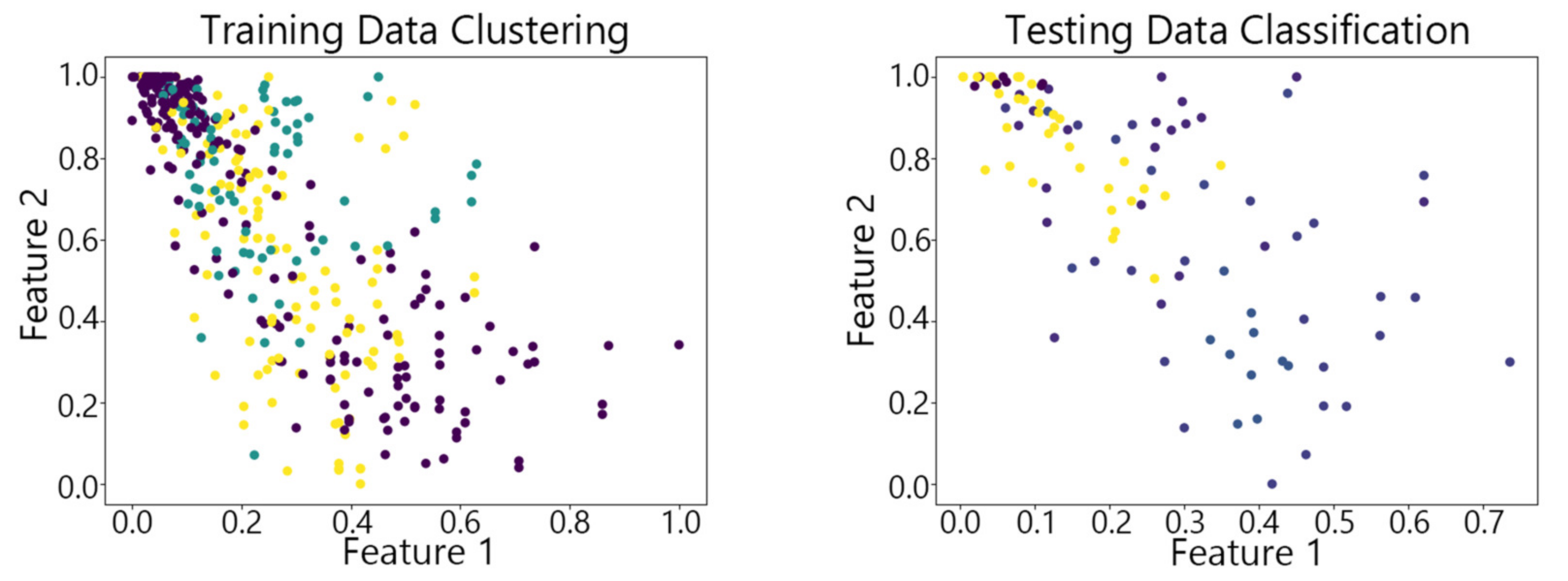
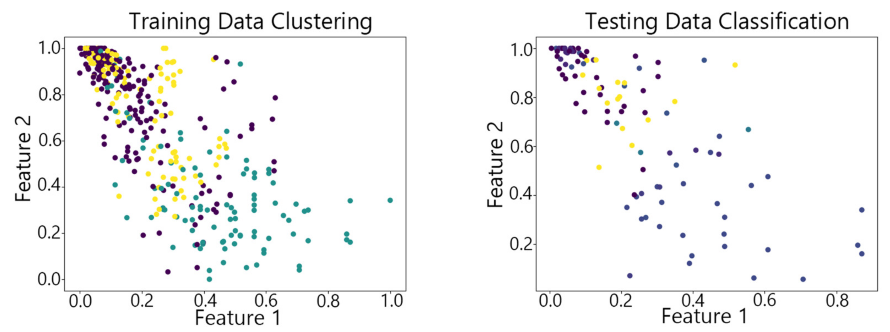
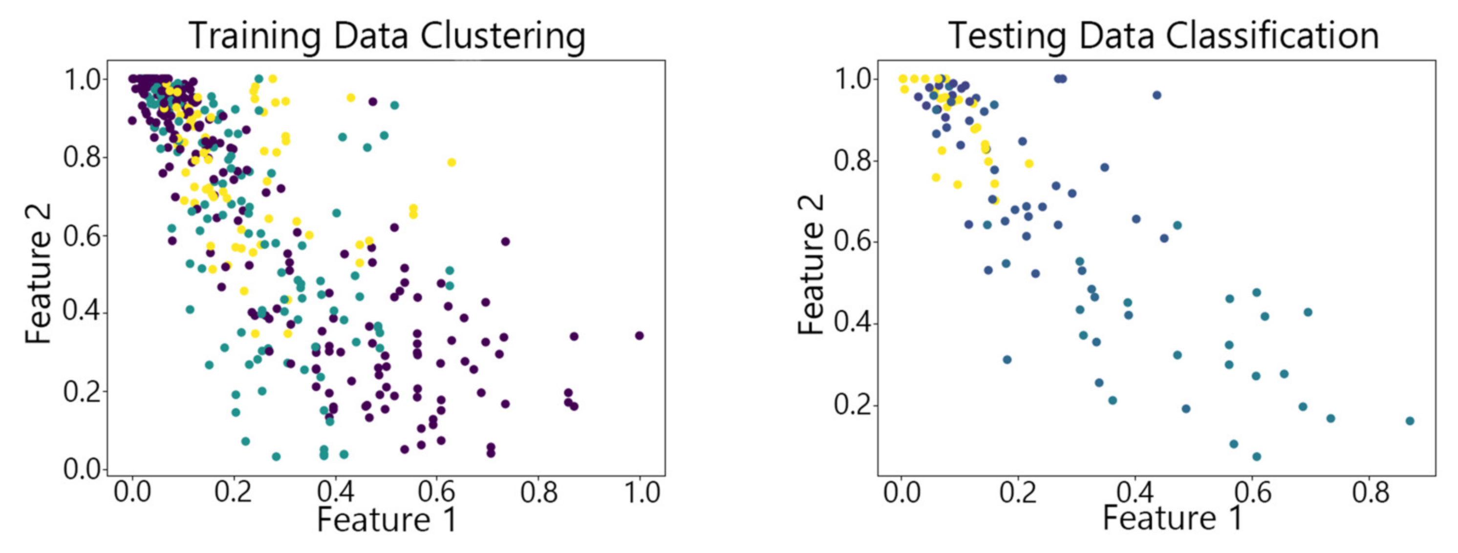
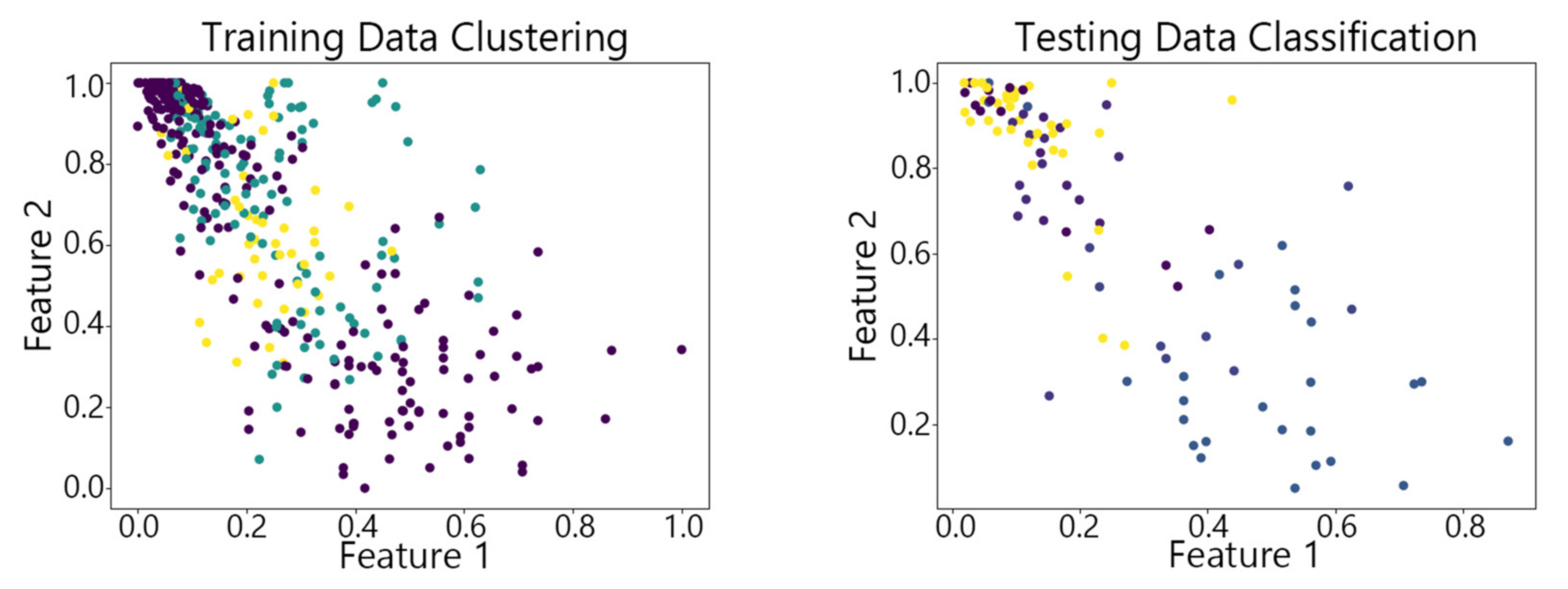
Figure 7, Figure 8,Figure 9, Figure 10 and Figure 11 show the clustering results of the SOM algorithm, the DBSCAN algorithm, the Hybrid SOM algorithm, the Dynamic Programming SOM(DP-SOM) algorithm, and the vwSOM algorithm on the training and testing sets of Iris. The clustering results of Wine using different algorithms are shown in Figure 12, Figure 13,Figure 14, Figure 15 and Figure 16. The clustering results of the Waveform dataset using different algorithms are shown in Figure 17, Figure 18,Figure 19, Figure 20 and Figure 21. To determine the position of the data in the clustering graph, we used the petal length and petal width as the horizontal and vertical axes because these two characteristics have a high linear correlation with the class and can better represent the class. Similarly, the alcohol and malic acid components in the wine better characterize the classes, so these two features are chosen as the axes for the scatter plot. The first feature in the Waveform dataset represents the signal’s amplitude, while the second feature represents the signal’s periodicity or frequency variations. These two features have the highest correlation, so they are used as the x-axis and y-axis in a scatter plot to represent the data distribution. Different colors in the clustering graph represent different clustering clusters.
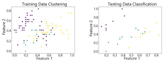
Figure 7.
The SOM algorithm on Iris.
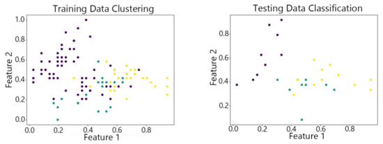
Figure 8.
The DBSCAN algorithm on Iris.
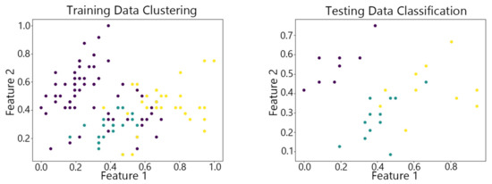
Figure 9.
The Hybrid SOM algorithm on Iris.
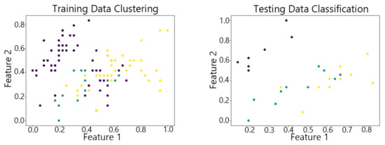
Figure 10.
The DP-SOM algorithm on Iris.
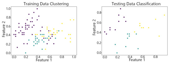
Figure 11.
The vwSOM algorithm on Iris.
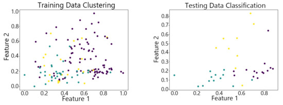
Figure 12.
The SOM algorithm on Wine.
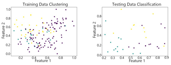
Figure 13.
The DBSCAN algorithm on Wine.
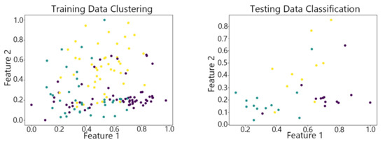
Figure 14.
The Hybrid SOM algorithm on Wine.
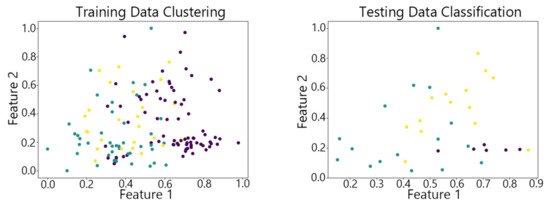
Figure 15.
The DP-SOM algorithm on Wine.
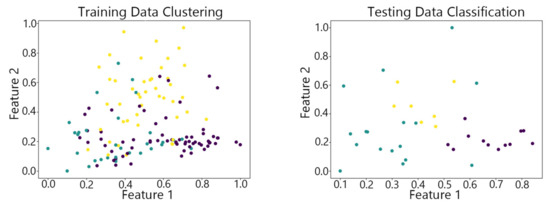
Figure 16.
The vwSOM algorithm on Wine.

Figure 17.
The SOM algorithm on Waveform.

Figure 18.
The DBSCAN algorithm on Waveform.
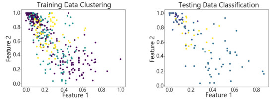
Figure 19.
The Hybrid SOM algorithm on Waveform.
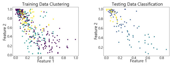
Figure 20.
The DP-SOM algorithm on Waveform.

Figure 21.
The vwSOM algorithm on Waveform.
By observing the scatter plots, it can be seen that when using highly correlated features to characterize the data, they exhibit different distribution characteristics, and different features determine the position of the data on the scatter plot. When training the model with the training set and inputting the test data to verify its clustering effect, it can be found that the test data are clustered into the same class as the training data with the same characteristics. This is consistent with the evaluation indicators obtained from the experimental results. The number of points presented in the scatter plot is slightly less than the number of training and testing data in the experimental code settings. This is due to the fact that some data will appear at the same position on the scatter plot when the petal length and width of different data are extremely close or completely identical. And due to their consistent characteristics, they will be clustered into the same category so that their color presented in the scatter plot will also be consistent.
4.3. Clustering Results of Different Algorithms
Table 5 shows the clustering results obtained by the SOM algorithm, the DBSCAN algorithm, the Hybrid SOM algorithm, and the vwSOM algorithm on the Iris dataset. The clustering results of different algorithms on the Wine dataset are shown in Table 6. The clustering results of different algorithms on the Waveform dataset are shown in Table 7. When dealing with complex data structures, using distance similarity alone for clustering may not yield satisfactory results. Therefore, based on the primitive SOM algorithm, the density similarity has emerged. DBSCAN is a classic density-based clustering algorithm that categorizes sample data into core points, boundary points, and outlier points based on their distribution density. It forms different clusters through definitions such as density-reachable, density-connected, and others. However, when dealing with larger datasets, it exhibits slow convergence and performs poorly when the dataset has an uneven density distribution. The Hybrid SOM algorithm combines the traditional SOM model with the KNN model. It trains the SOM on a healthy dataset with minimal noise. After fitting the healthy data, nodes that are too sparse or fall below the minimum BMU threshold are removed to prevent BMU contamination by noise. Then, a layer of KNN is added after the SOM model to identify data based on the Euclidean distance between centroids and observed data points. Test data are input into the trained KNN to detect outliers based on the Euclidean distance between the test data and nodes within the cluster. Classification using SOM based on Dynamic Programming entails utilizing a neural network framework to arrange and categorize input data within a two-dimensional grid, clustering similar data points together. By integrating the self-organizing properties of SOMs with Dynamic Programming methods, the neuron assignment of input data is maximized, and the classification process can be optimized.
Table 5.
Comparison of clustering effects of different algorithms on the Iris dataset.
Table 6.
Comparison of clustering effects of different algorithms on the Wine dataset.
Table 7.
Comparison of clustering effects of different algorithms on the Waveform Dataset.
Due to the weak boundary characteristics between classes in the Iris dataset, it is challenging to choose hyperparameters for the DBSCAN algorithm. This makes it difficult to determine cluster sizes and identify boundary points. As a result, its S, F1 score and ACC are 0.5062, 0.84 and 0.88, respectively, which are all lower than those of the vwSOM algorithm. Due to the uneven sample distribution, the clustering analysis of the Wine dataset using this algorithm results in a decreased ACC value and an increased VA value, indicating a reduction in clustering stability. However, it is easy to implement because of the low complexity. And with a processing time of only 0.0244ms for the individual data of Iris, this algorithm is suitable for real-time data processing scenarios with low precision requirements.
When applied to clustering the Iris dataset, the Hybrid SOM algorithm yields an S of 0.5235, an ACC of 0.9395, and an F1 score of 0.91, lower than the results of the vwSOM algorithm due to its relatively low R-value, indicating a higher number of false negative predictions. When processing the Wine dataset, the ACC value slightly decreases. The Hybrid SOM algorithm exhibits good scalability through threshold judgment and reduces computation time and algorithm complexity but may also result in the loss of some valid information.
When the DP-SOM algorithm handles datasets with fewer features, it does not show a significant advantage in terms of accuracy. However, when the dataset has a larger number of features, such as the Wine and Waveform datasets, the DP-SOM algorithm, due to its ability to dynamically program the allocation of neurons, adjusts the neuron weights to be closer to the input data. As a result, the algorithm’s accuracy is higher than that of the hybrid SOM algorithm, while its accuracy is very close to that of the vwSOM algorithm.
The vwSOM algorithm on Iris achieves an S of 0.5262, an F1 score of 0.93 and an ACC of 0.9412, with a relatively low VA value, indicating high clustering accuracy and stable performance. When used for clustering the Wine dataset, the S is 0.5255, the F1 score remains at 0.93, and the ACC and VA values are essentially unchanged. This indicates that the uneven distribution of samples across different classes in the dataset has a minimal impact on the vwSOM algorithm. The algorithm processes the individual data of the Iris in 0.2221 ms and 0.2263 ms of the Wine. The AOT value increases with the number of data features. Although it is slightly higher than the AOT of the above two algorithms, it meets the real-time data processing requirements. It strikes a good balance between algorithm complexity and computational accuracy, making it suitable for practical data anomaly handling in real-life scenarios. When the vwSOM algorithm is applied to the Waveform dataset, the S, the F1 score and accuracy decrease, with values of 0.5101, 0.88 and 0.8931, respectively. This is due to the Waveform dataset being a large-scale, multi-feature dataset. During the training process of the model’s weight matrix, different feature vectors influence each other, which reduces the representation capability of the neuron nodes for the mapped data, thus affecting the final training results. Additionally, the large number of features in the sample data increases the time required to process each individual data point. However, when compared to the experimental results of other algorithms on the same dataset, the proposed algorithm still shows advantages in terms of clustering accuracy and stability.
4.4. Ablation Experiments
The vwSOM model is based on the SOM model and uses the PCA algorithm to initialize the weight matrix, as well as adding virtual winning neurons to transform the traditional single winning neuron mechanism into a multi-winning mechanism. Through ablation experiments, the roles of each module of the vwSOM algorithm in terms of accuracy and stability are observed, as shown in Table 8.
Table 8.
Ablation experiments.
For example, when processing the Iris dataset, the SOM algorithm has an ACC of 0.8986, VA of 0.0026, and a relatively low R value of 0.85. By using the PCA algorithm to determine the direction of maximum variance in the dataset, it provides a good starting point for subsequent model training. Each principal component serves as an initial weight vector for initializing the SOM model’s weight matrix. This approach accelerates the convergence of the algorithm. The P value is relatively high at 0.8999, and the ACC is improved. Additionally, the VA significantly decreases to 0.0017, indicating an enhancement in algorithm stability. By innovating the single winning neuron mechanism in the SOM algorithm and introducing the concept of virtual winning neurons, the algorithm achieves a higher F1 score and a noticeable increase in ACC to 0.9385. The VA value is 0.0020, lower than the traditional algorithm. This is because changing the number of winning neurons allows for capturing more information with minimal errors, enabling a more comprehensive representation of the input data features. Analyzing the experimental data reveals that PCA enhances algorithm stability. The idea of virtual winning neurons derived from multiple winning neurons contributes to improving algorithm accuracy. Combining these enhancements and applying them to the SOM yields the vwSOM algorithm, with an F1 score of 0.93, an ACC of 0.9412, and a VA of 0.0012, indicating high accuracy and good stability of the algorithm.
5. Conclusions
This paper innovates on the classic unsupervised learning SOM model by using the PCA algorithm to initialize the weight matrix. It also improves the single winning neuron mechanism to multiple winning neurons, and proposes the concept of virtual neuron nodes. The proposed vwSOM algorithm can be used for anomaly detection in data transmission within communication systems by inputting certain data into a trained model. If the data cannot be clustered into any category, the point is considered an anomaly. A clustering analysis of the Iris dataset and the Wine dataset using the vwSOM algorithm shows that the proposed algorithm achieves better clustering results with high accuracy. It also reduces sensitivity to input data and exhibits good stability. Additionally, the experimental results show that the vwSOM algorithm has strong generalization ability and can be widely applied in data processing of dynamic systems. It is capable of handling the high-dimensional and complex data commonly found in dynamical systems. This efficiency enables the rapid identification of patterns and structures within the data. For instance, vwSOM can assist in mapping these interactions and comprehending their influence on the overall system behavior, which is crucial for understanding the underlying dynamical systems. Although the vwSOM model has the aforementioned advantages in practical anomaly detection applications, there is still room for improvement. During the training process, this model maps data from different categories to the same weight matrix, which may lead to mutual influence between them. Whether it is possible to train each category of data separately to achieve higher clustering accuracy is a topic worth exploring.
Author Contributions
Methodology, X.F., S.Z. and X.X.; Writing—original draft, S.F.; Writing—review & editing, R.J. and H.K.; Supervision, X.F., S.Z., X.X. and R.J. All authors have read and agreed to the published version of the manuscript.
Funding
This project was funded by the National Natural Science Foundation of China under Grant 62371246 and 62271266.
Data Availability Statement
Data are contained within the article.
Acknowledgments
The authors thank SDIC Gansu Xiaosanxia Power Co., Ltd. and Nanjing University of Posts and Telecommunications for its continued support.
Conflicts of Interest
The authors Xiaoliang Fan, Shaodong Zhang and Xuefeng Xue were employed by the company SDIC Gansu Xiaosanxia Power Co., Ltd. The remaining authors declare that the research was conducted in the absence of any commercial or financial relationships that could be construed as a potential conflict of interest.
References
- Zhou, Z. Machine Learning; Tsinghua University Press: Beijing, China, 2016. [Google Scholar]
- Li, Y.; Li, H.; Qian, X.; Zhu, Y. A review and analysis of outlier detection algorithms. Comput. Eng. 2002, 28, 5–6+32. [Google Scholar]
- Xu, X.; Liu, H.; Yao, M. Recent Progress of Anomaly Detection. Complexity 2019, 2019, 1–11. [Google Scholar] [CrossRef]
- Omar, S.; Ngadi, A.; Jebur, H.H. Machine Learning Techniques for Anomaly Detection: An Overview. Int. J. Comput. Appl. 2013, 79, 3–41. [Google Scholar] [CrossRef]
- Nassif, A.B.; Talib, M.A.; Nasir, Q.; Dakalbab, F.M. Machine Learning for Anomaly Detection: A Systematic Review. IEEE Access 2021, 9, 78658–78700. [Google Scholar] [CrossRef]
- Bzdok, D.; Krzywinski, M.; Altman, N. Machine learning: Supervised methods. Nat. Methods 2018, 15, 5–6. [Google Scholar] [CrossRef] [PubMed]
- Ester, M.; Kriegel, H.P.; Sander, J.; Xu, X. A density-based algorithm for discovering clusters in large spatial databases with noise. In Proceedings of the Second International Conference on Knowledge Discovery and Data Mining (KDD’96), Portland, OR, USA, 2–4 August 1996; pp. 226–231. [Google Scholar]
- Goldstein, M.; Uchida, S. A comparative evaluation of unsupervised anomaly detection algorithms for multivariate data. PLoS ONE 2016, 11, 1–15. [Google Scholar] [CrossRef] [PubMed]
- Gadal, S.; Mokhtar, R.; Abdelhaq, M.; Alsaqour, R.; Ali, E.S.; Saeed, R. Machine Learning-Based Anomaly Detection Using K-Mean Array and Sequential Minimal Optimization. Electronics 2022, 11, 2158. [Google Scholar] [CrossRef]
- Jain, M.; Kaur, G.; Saxena, V. A K-Means clustering and SVM based hybrid concept drift detection technique for network anomaly detection. Expert Syst. Appl. 2022, 193, 116510. [Google Scholar] [CrossRef]
- Dai, Y.; Sun, S.; Che, L. Improved DBSCAN-based Data Anomaly Detection Approach for Battery Energy Storage Stations. J. Phys. Conf. Ser. 2022, 2351, 012025. [Google Scholar] [CrossRef]
- Zhang, L.; Liu, L. Data anomaly detection based on isolation forest algorithm. In Proceedings of the 2022 International Conference on Computation, Big-Data and Engineering (ICCBE), Yunlin, Taiwan, 27–29 May 2022; pp. 87–89. [Google Scholar]
- Kohonen, T. The Self-Organizing Map. Proc. IEEE 1990, 78, 1464–1480. [Google Scholar] [CrossRef]
- Kohonen, T. Things you haven’t heard about the Self-Organizing Map. In Proceedings of the IEEE international Conference on Neural Networks, San Francisco, CA, USA, 28 March–1 April 1993; pp. 1147–1156. [Google Scholar]
- Kohonen, T. Exploration of very large databases by Self-Organizing Maps. In Proceedings of International Conference on Neural Networks (icnn’97), Houston, TX, USA, 12 June 1997; pp. PL1–PL6. [Google Scholar]
- Kohonen, T. Essentials of the Self-Organizing Map. Neural Netw. 2013, 37, 52–65. [Google Scholar] [CrossRef] [PubMed]
- Sandoval-Lara, Z.; Gómez-Gil, P.; Moreno-Rodríguez, J.C.; Ramírez-Cortés, M. Self-Organizing Clustering by Growing-SOM for EEG-Based Biometrics. In Proceedings of the 2023 International Conference on Artificial Intelligence and Applications (ICAIA) Alliance Technology Conference (ATCON-1), Bangalore, India, 21–22 April 2023; pp. 1–4. [Google Scholar]
- Cui, W.; Xue, W.; Li, L.; Shi, J. A Method for Intermittent Fault Diagnosis of Electronic Equipment Based on Labeled SOM. In In Proceedings of the 2020 International Conference on Sensing, Diagnostics, Prognostics, and Control (SDPC), Beijing, China, 5–7 August 2020; pp. 149–154. [Google Scholar]
- Zhang, X.; Xu, J.; Zhang, H. Fault Diagnosis of Levitation Controller of Medium-Speed Maglev Train Based on SOM-BP Neural Network. In Proceedings of the 2023 35th Chinese Control and Decision Conference (CCDC), Yichang, China, 20–22 May 2023; pp. 4162–4167. [Google Scholar]
- Chen, S.; Liu, Z.; Zhou, H.; Wen, X.; Xue, Y. Seismic Facies Visualization Analysis Method of SOM Corrected by Uniform Manifold Approximation and Projection. IEEE Geosci. Remote. Sens. Lett. 2023, 20, 1–5. [Google Scholar] [CrossRef]
- Kuncheva, L.I.; Faithfull, W.J. PCA Feature Extraction for Change Detection in Multidimensional Unlabeled Data. IEEE Trans. Neural Networks Learn. Syst. 2014, 25, 69–80. [Google Scholar] [CrossRef] [PubMed]
- Anderson, E. The Irises of the Gaspe Peninsula. Bull. Am. Iris Soc. 1935, 59, 2–5. [Google Scholar]
- Aeberhard, S.; Coomans, D.; de Vel, O. Comparison of Classifiers in High Dimensional Settings; Technical Report; Department of Mathematics and Statistics, James Cook University: North Queensland, Australia, 1992; Volume 92. [Google Scholar]
- Aha, D.W.; Kibler, D. Instance-based learning algorithms. Mach. Learn. 1991, 6, 37–66. [Google Scholar] [CrossRef]
- Khan, S.; Mailewa, A.B. Discover botnets in IoT sensor networks: A lightweight deep learning framework with hybrid Self-Organizing Maps. Microprocess. Microsystems 2023, 97, 104753. [Google Scholar] [CrossRef]
- Manikant, M.N. Improved Classification of Cyber-Bullying Tweets in Social Media Using SVM-MaxEnt Based Dynamic Programming Based Self Organizing Maps. In Proceedings of the 2024 13th International Conference on System Modeling & Advancement in Research Trends (SMART), Moradabad, India, 6–7 December 2024; pp. 99–106. [Google Scholar]


Disclaimer/Publisher’s Note: The statements, opinions and data contained in all publications are solely those of the individual author(s) and contributor(s) and not of MDPI and/or the editor(s). MDPI and/or the editor(s) disclaim responsibility for any injury to people or property resulting from any ideas, methods, instructions or products referred to in the content. |
© 2025 by the authors. Licensee MDPI, Basel, Switzerland. This article is an open access article distributed under the terms and conditions of the Creative Commons Attribution (CC BY) license (https://creativecommons.org/licenses/by/4.0/).