Modeling of Flow-Difference Influences on Dynamic Phase Transition and Stability in Curved Road Traffic Systems

Abstract

The traffic flow difference factor is of great significance for traffic flow stability and congestion mitigation. However, its role has not been studied in existing curved-road traffic flow models. To fill this gap, this study proposes an improved lattice traffic flow model for curved roads based on lattice hydrodynamic theory, which comprehensively considers the synergistic influence of curve geometric characteristics and the flow difference factor on traffic dynamics. Meanwhile, the new model adopts a modified optimal speed function regarding the symmetric characteristics of density. Through linear stability analysis, the stability criterion of the new model is derived. Via nonlinear analysis, the mKdV equation describing the propagation mechanism of traffic congestion near the critical point, along with its density wave solution, is obtained. The results show that introducing the traffic flow difference factor can significantly suppress the propagation speed and fluctuation amplitude of density waves and reduce the driver’s critical sensitivity coefficient, thereby effectively enhancing the stability and robustness of traffic flow on curved roads. Moreover, the model’s stability gradually improves as the curve curvature increases. Under the same curve conditions, compared with the classical Zhou model, the critical sensitivity and density wave propagation speed of the new model are reduced by approximately 16.67% and 19.48%, respectively, with favorable traffic congestion suppression effects.

1. Introduction

Traffic flow theory primarily investigates the formation, motion laws, and dynamic characteristics of traffic flow on roadways. It establishes models through mathematical, physical, and statistical methods to reveal the relationships between various traffic flow parameters, explain the causes of traffic phenomena (such as congestion, bottlenecks, and accidents), and predict the evolutionary trends of traffic flow. In recent years, traffic flow theory has attracted extensive attention from scholars with diverse backgrounds, leading to the successive proposal of a series of traffic flow models [1,2,3,4,5,6,7,8]. Among these models, one category, known as microscopic traffic flow models, takes individual vehicles as the modeling object and mainly depicts the interaction rules between vehicles. Representative models include cellular automaton models [1,2] and car-following models [3,4]. The other category, referred to as macroscopic traffic flow models, adopts the overall traffic flow as the modeling scale and describes the spatiotemporal evolution laws of the entire traffic flow. Typical models include continuous models [5,6] and lattice models [7,8].

In the field of traffic flow research, how to construct accurate and effective theoretical models has always been a focus of academic attention. In 1998, scholar Nagatani [7] made a breakthrough by combining the analysis of macroscopic overall traffic conditions with the study of microscopic individual vehicle behaviors, proposing a single-lane lattice traffic flow model. Based on this model, Nagatani [8] further considered the ubiquitous lane-changing behaviors in actual traffic, expanding the single-lane model into a two-lane lattice framework. Since the mKdV (modified Korteweg-de Vries) density equation describing the evolution process of traffic congestion can be derived relatively simply from Nagatani’s single-lane [7] and two-lane lattice models [8], the Nagatani model has rapidly gained widespread attention in the field of traffic flow research. However, in the construction process of Nagatani’s lattice models [7,8], many key factors affecting traffic flow were simplified to facilitate mathematical treatment and theoretical derivation. Although these simplifications endow the model with a concise mathematical form and high computational efficiency, they also make it difficult to accurately simulate complex scenarios in the real traffic environment. To break through these limitations and better reproduce the rich nonlinear phenomena in complex traffic systems, researchers have carried out a large number of extension studies around the Nagatani model. Factors such as driver prediction effects [9,10,11,12], traffic jerk effects [13], curve overtaking [14,15,16], honking effects [17,18], ramp effects [19,20,21,22], and self-stabilizing effects [23,24] have been successively introduced. These extensions have greatly enriched the theoretical connotation of the Nagatani model and significantly improved its adaptability to complex traffic scenarios and prediction accuracy.

Notably, most existing traffic flow lattice models are designed for straight roads, limiting their ability to accurately capture the dynamic characteristics of curved-road traffic. In curved scenarios, beyond road geometric alignment, centrifugal force exerts a substantial influence on vehicle operation. According to automotive dynamics principles, when a vehicle travels on a curve, centrifugal force increases as the turning radius decreases or the driving speed increases. This not only elevates the demand for lateral tire friction—thereby restricting the safe driving speed—but also prolongs drivers’ reaction time and vehicles’ braking distance, exacerbating the cumulative effect of speed differences between vehicles and ultimately amplifying the instability of traffic flow. Therefore, how to extend traffic flow models developed for straight roads to curved road scenarios by integrating the characteristics of curves and vehicle dynamics has become a key research focus in the field of traffic flow. In 2015, Cao and Shi [25] pioneered a curved lattice model to explore the influence of friction coefficients and curvature radii on traffic flow characteristics. One year later, Zhou and Shi [26] further enhanced this model by integrating the effects of curve arcs. Concurrently, Zhou et al. [27] developed a curved-road adaptation of Nagatani’s two-lane lattice model in 2016. Thereafter, in 2025, Xiao et al. [28] proposed a novel lattice hydrodynamic model on curved roads with the empirical lane-changing rate. Wang et al. [29] in 2020 put forward a novel lattice hydrodynamic model for curved road scenarios, which incorporates the effects of drivers’ memory and differences in optimal speed. Cheng et al. [30] in 2019 explored the role of delayed feedback control in curved road scenarios. Mehta et al. [31] in 2025 investigated the dynamic characteristics of traffic flow on curved roads by incorporating the impacts of visibility and lane-changing maneuvers and developed a new lattice model. Wang et al. [32] in 2025 constructed a unified lattice hydrodynamic model integrating straight, curved, and sloped segments.

Existing studies [33,34,35,36] have confirmed that flow difference information—defined as the difference between the traffic flows passing through adjacent lattice units per unit time—exerts a significant regulatory effect on traffic dynamics characteristics. However, based on current understanding, the lattice traffic flow models for curved roads have not yet incorporated this factor into the research scope. Therefore, under the constraint of the unique alignment structure of curved roads, the action pathway of flow difference on traffic flow remains theoretically unexplored. From a mechanistic perspective, the flow difference in lattice traffic flow models and the speed difference in car-following models [37,38] exhibit similar regulatory functions: both can provide dynamic decision-making bases for drivers within the current lattice, guiding them to adjust their driving strategies accordingly. However, it should be explicitly noted that there exists a significant discrepancy in their modeling scales: the flow difference in lattice models reflects the overall dynamic imbalance of macroscopic traffic flow between adjacent road segments, with its regulatory target being all vehicles within a specific lattice; in contrast, the speed difference in car-following models focuses on the movement relationship between an individual vehicle and its preceding vehicle, and its regulatory target is the driving behavior of a single driver. Notably, leveraging the real-time data interaction capability of Cyber-Physical Systems (CPS) and through the real-time communication technology between Road-Side Units (RSUs) and On-Board Units (OBUs) of intelligent connected vehicles, drivers in curved road scenarios can obtain real-time interactive information such as flow differences, thereby enabling them to predict changes in the preceding traffic flow in advance. This provides robust data support for the optimization of driving decisions and the optimal control of traffic flow on curved roads. To accurately reveal the interactive influence mechanism of flow difference and geometric characteristics of curved roads on traffic flow, and meanwhile bridge the existing research gap, we embedded a flow difference effect module into the model proposed by Zhou et al. [26] to construct a new lattice traffic flow model for curved roads. Through theoretical analysis and numerical simulation, the collaborative action mechanism of flow difference and geometric characteristic parameters of curved roads on the evolution of traffic flow on curved roads was systematically explored.

The main contributions of this paper are as follows: (1) Although the flow difference effect has been widely mentioned in straight road traffic research, there is currently no systematic study on it in curved road scenarios. Therefore, this study extends the research on the flow difference effect from straight roads to more complex curved road scenarios, which possess clear scenario-specific innovative value. (2) The linear stability criterion of the new model for curved road scenarios and the density wave evolution equation describing the propagation law of traffic congestion near the critical point are derived, providing a quantitative tool for the theoretical analysis of curved road traffic flow under the influence of the flow difference factor. (3) Both numerical simulations and theoretical analyses consistently show that the introduced flow difference information has a stabilizing effect and congestion suppression capability on traffic flow in curves. It is also confirmed that the stability of traffic flow in curves increases with the increase in road radius.

2. Models

2.1. Classical Single-Lane Nagatani Lattice Model

In 1998, Nagatani [7] pioneered the development of a lattice model to characterize the evolution process of macroscopic traffic streams under the scenario of a single-lane roadway. The governing equations of this model are given as follows:

$${\mathsf{\partial }}_t{\rho }_j(t)+{\rho }_0[{\rho }_j(t)v_j(t)-{\rho }_{j-1}(t)v_{j-1}(t)]=0$$

(1)

$${\rho }_j(t+\tau )v_j(t+\tau )={\rho }_{0}V({\rho }_{j+1}(t))$$

(2)

Here, symbol j denotes the index of the road segment (lattice). Variables ${\rho }_j(t)$ and $v_j(t)$ represent the average density and speed of the macroscopic traffic flow on the j-th segment at time $t$, respectively. ${\rho }_0$ is the overall average density of traffic flow in the entire transportation system, and it is inversely proportional to the average headway δ, i.e., $\delta =1/{\rho }_0$. The parameter $\tau$ stands for the reaction delay of drivers, which is inversely proportional to the driver sensitivity coefficient $a$, i.e., $\tau = 1/a$. $V$, meanwhile, denotes the optimal velocity function. Considering the symmetry of density, the optimal velocity function in the Nagatani lattice model is given by [39]:

$$V({\rho }_j)={\displaystyle \frac{V_{\max }}{2}}\tanh ({\displaystyle \frac{2}{{\rho }_0}}-{\displaystyle \frac{{\rho }_j(t)}{{\rho }_0^2}}-{\displaystyle \frac{1}{{\rho }_c}})+\tanh ({\displaystyle \frac{1}{{\rho }_c}})$$

(3)

where ${\rho }_c$ represents the critical density value, and $v_{max}$ is the maximum speed of the vehicle. When ${\rho }_0={\rho }_c$, Equation (3) has an inflection point at ${\rho }_j={\rho }_c$.

2.2. Classical Single-Lane Curved Road Lattice Model

Figure 1 depicts an abstract physical model of a curved road. R is the road’s radius of curvature, and ${\theta }_j$ denotes the radian corresponding to the $j$-th lattice point. The road curvature is defined by $y=\sqrt{R^2-(x-R{)}^2}$. The arc length between adjacent lattice points ($j$ and $j$ − 1) is calculated as [26]:

$$l={\displaystyle {\int }_{x-x_0}^x\sqrt{1+y^{’2}}}dx={\displaystyle \frac{x_0}{\sin {\theta }_j}}$$

(4)

For the traffic flow scenario of the curved road illustrated in Figure 1, Zhou and Shi [26] improved the classical Nagatani single-lane lattice model based on Equation (4) and proposed a corresponding lattice model for curved roads, whose governing equations are given as follows:

$${\mathsf{\partial }}_t{\rho }_j(t)+{\displaystyle \frac{{\rho }_0}{\sin {\theta }_j}}[{\rho }_j(t)v_j(t)-{\rho }_{j-1}(t)v_{j-1}(t)]=0$$

(5)

$${\rho }_j(t+\tau )v_j(t+\tau )={\displaystyle \frac{{\rho }_0}{\sin {\theta }_j}}V({\rho }_{j+1}(t))$$

(6)

Equation (5) characterizes the conservation of vehicle count under the curved road traffic scenario and is thus termed the vehicle conservation equation. Equation (6) is referred to as the motion equation that describes the vehicular movement characteristics. To accommodate the curved road scenario, the optimal velocity function Equation (3) has also been revised, taking the following form [26]:

$$V({\rho }_j)=\beta {\displaystyle \frac{\sqrt{\mu gR}}{2}}[\tanh ({\displaystyle \frac{2}{{\rho }_0}}-{\displaystyle \frac{{\rho }_j}{{\rho }_0^2}}-{\displaystyle \frac{1}{{\rho }_c}})+\tanh ({\displaystyle \frac{1}{{\rho }_c}})]$$

(7)

Here, parameters $\mu$ and $g$ denote the road surface friction coefficient and gravitational acceleration, respectively. For safety considerations, vehicle speeds on curved sections are significantly lower than the theoretical maximum speed $V_{max}=\sqrt{\mu gR}$ and, thus, a control coefficient $\beta$ is introduced.

2.3. The New Model

Recent research achievements [33,34,35,36] have confirmed that the flow difference between adjacent grid points significantly modulates the dynamic evolution process of macroscopic traffic flow. In contrast, the existing lattice models for curved road traffic flow [11,14,28,29,30] rarely incorporate the influence mechanism of traffic flow difference effects in their modeling frameworks. Especially in curved road scenarios, the collaborative effect of flow difference and road geometric curvature on the stability of traffic flow has not been fully analyzed. To break through this theoretical bottleneck, drawing on the modeling idea from the literature [40], this study introduces a flow difference effect term based on the basic lattice model framework proposed by Zhou et al. [26] and constructs an improved traffic flow dynamics model adaptable to curved roads. The evolution equation of this new model is as follows:

$${\rho }_j(t+\tau )-{\rho }_j(t)+{\displaystyle \frac{1}{\sin {\theta }_j}}\tau {\rho }_0[{\rho }_j(t)v_j(t)-{\rho }_{j-1}(t)v_{j-1}(t)]=0$$

(8)

$${\rho }_j(t+\tau )v_j(t+\tau )={\displaystyle \frac{1}{\sin {\theta }_j}}{\rho }_{0}V({\rho }_{j+1}(t))+k[{\rho }_{j+1}(t)v_{j+1}(t)-{\rho }_j(t)v_j(t)]$$

(9)

Here, ${\rho }_j(t)v_j(t)$ denotes the traffic flow on the j-th road segment at time t. The term $\Delta Q_j(t)={\rho }_{j+1}(t)v_{j+1}(t)-{\rho }_j(t)v_j(t)$ represents the introduced traffic flow difference information at grid point j at time t, and parameter $k$ is the corresponding response intensity coefficient. When $k$ = 0, the proposed model in this paper degenerates into the model by Zhou et al. [26]; thus, the latter is a special case of the proposed model. From the perspective of driving behavior mechanisms, drivers typically exhibit a gradual response to flow differences, with the magnitude of their adjustments approximating a linear correlation with these differences. Consequently, the new model employs a linear term to simplify the description of this regularity. Furthermore, while the driver response coefficient $k$ is associated with the road’s radius of curvature, $k$ is temporarily set as a constant in the model to focus on core mechanisms. It should be noted that the linear flow difference term in Equation (9) cannot capture the saturated response characteristics of drivers under extreme conditions (e.g., when flow differences are excessively large).

Eliminating the speed variable $v$ in Equations (8) and (9), we obtain the evolution equation about the density variable:

$$\begin{array}{l}{\rho }_j(t+2\tau )-{\rho }_j(t+\tau )+{\displaystyle \frac{1}{{\sin }^2{\theta }_j}}\tau {\rho }_0^2[V({\rho }_{j+1}(t))-V({\rho }_j(t))]\\ -k[\Delta {\rho }_j(t+\tau )-\Delta {\rho }_j(t)]=0\end{array}$$

(10)

in which $\Delta {\rho }_j={\rho }_{j+1}-{\rho }_j$.

3. Linear Stability Analysis

At the initial moment, it is assumed that the traffic density at all lattices is uniformly distributed as ${\rho }_0$ and maintains a consistent moving speed $V({\rho }_0)$. Under such circumstances, the steady-state solution of Equation (10) is as follows:

$${\rho }_j(t)={\rho }_0,v_j(t)=V({\rho }_0)$$

(11)

A small disturbance $y_j(t)$ is imposed on the steady state, and we have

$${\rho }_j(t)={\rho }_0+y_j(t)$$

(12)

Substituting (12) into (10) and linearizing yields:

$$\begin{array}{l}{y}_j(t+2\tau )-y_j(t+\tau )+{\displaystyle \frac{1}{{\sin }^2{\theta }_j}}\tau {\rho }_0^2{V}^{\prime }\Delta y_j(t)\\ -k[\Delta y_j(t+\tau )-\Delta y_j(t)]=0\end{array}$$

(13)

where $\Delta y_j=y_{j+1}-y_j$, $V^{’}={\displaystyle \frac{dV\left(\rho \right)}{d\rho }}{|}_{\rho ={\rho }_0}$. Expand $y_j(t)$ in Equation (13) into the form of a Fourier series: $y_j(t)=\mathit{exp}(ikj+zt)$, and the following expression can be obtained:

$$e^{2\tau z}-e^{\tau z}+{\displaystyle \frac{1}{{\sin }^2{\theta }_j}}\tau {\rho }_0^2{V}^{\prime }(e^{ik}-1)-k(e^{\tau z}-1)(e^{ik}-1)=0$$

(14)

Substituting $z=z_{1}ik+z_2(ik{)}^2$ into Equation (14) gives first- and second-order terms in $ik$:

$$z_1=-{\displaystyle \frac{1}{{\sin }^2{\theta }_j}}{\rho }_0^2{V}^{\prime },$$

(15)

$$z_2=-{\displaystyle \frac{3}{2{\sin }^4{\theta }_j}}\tau {({\rho }_0^2{V}^{\prime })}^2-(k+{\displaystyle \frac{1}{2}}){\displaystyle \frac{1}{{\sin }^2{\theta }_j}}{\rho }_0^2{V}^{\prime }$$

(16)

According to the judgment criteria of the long-wave expansion analysis method, if $z_2<0$, the traffic flow is unstable. Conversely, when z₂ > 0, the traffic flow is stable. Therefore, the critical stability condition of the new model is

$$\tau =-{\displaystyle \frac{(1+2k){\sin }^2{\theta }_j}{3{\rho }_0^2{V}^{\prime }}}$$

(17)

Hence, the stability condition of the proposed model is

$$\tau <-{\displaystyle \frac{(1+2k){\sin }^2{\theta }_j}{3{\rho }_0^2{V}^{\prime }}}$$

(18)

When $k=0$, the stability condition reduces to Zhou’s stability condition [26]:

$$\tau <-{\displaystyle \frac{{\sin }^2{\theta }_j}{3{\rho }_0^2{V}^{\prime }}}$$

(19)

In the proposed model, the stability condition of Equation (18) indicates that the flow difference response coefficient $k$ and road radian ${\theta }_j$ play a crucial role in determining the stability of traffic flow on curved roads. As shown in Figure 1, the arc length between lattice sites $j-1$ and $j$ is denoted as $\Delta s=l$, and the corresponding change in angle is $\Delta \theta ={\theta }_j-{\theta }_{j-1}$. According to the arc length formula, the relation $l=\Delta \mathrm{s}=R\Delta {\theta }_j$ holds. Given that the road curvature is $\epsilon ={\displaystyle \frac{1}{R}}$, substituting $R$ into this formula yields $\epsilon ={\displaystyle \frac{\Delta {\theta }_j}{\Delta s}}$. As $\Delta s\to 0$, taking the limit gives $\epsilon =\underset{\Delta s\to 0}{lim}{\displaystyle \frac{\Delta {\theta }_j}{\Delta s}}={\displaystyle \frac{d{\theta }_j}{ds}}$. It can thus be seen that the parameter ${\theta }_j$ in the new model has a corresponding relationship with the variable $\epsilon$ that describes the road curvature and can be used to characterize the degree of curvature of a curved road.

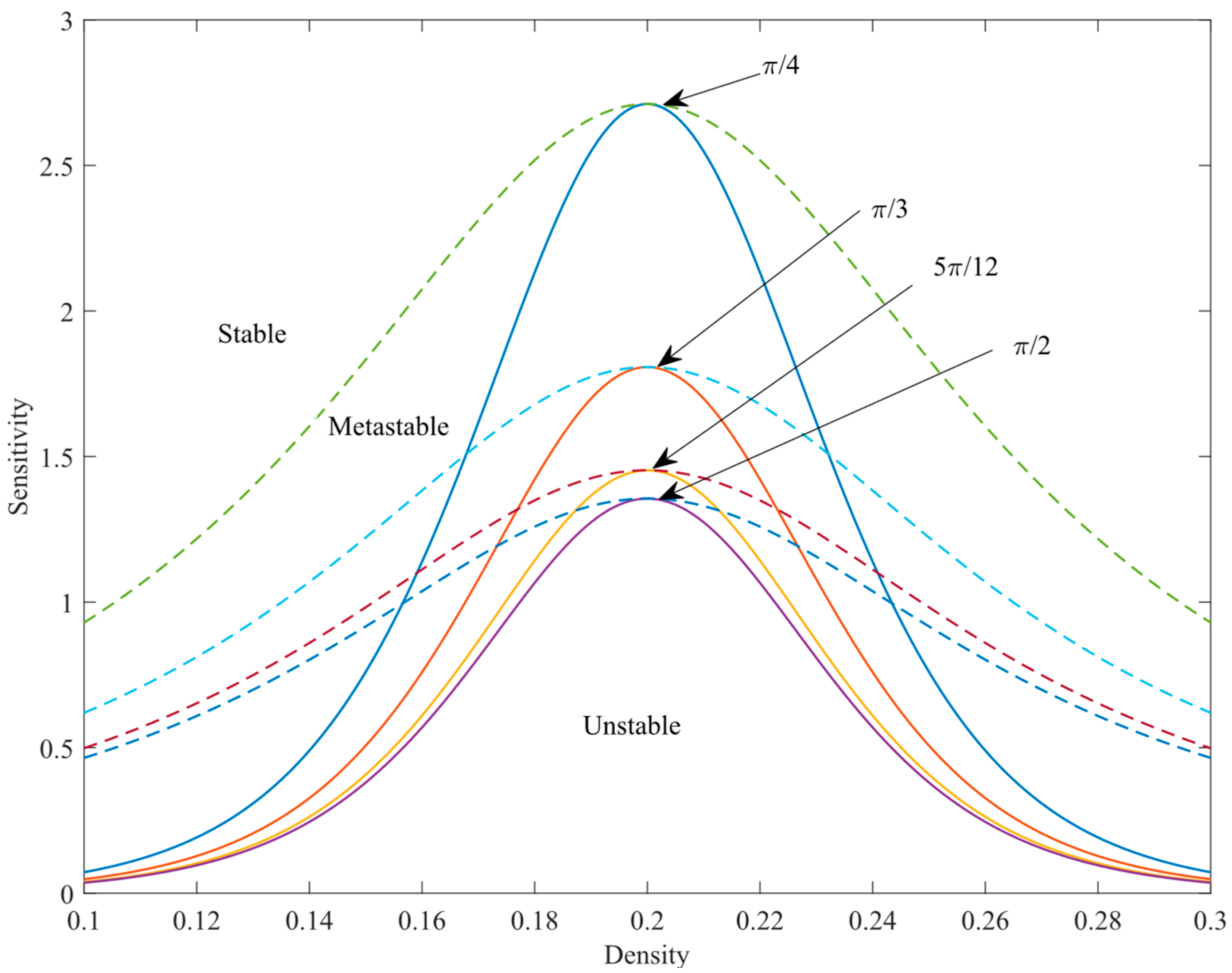
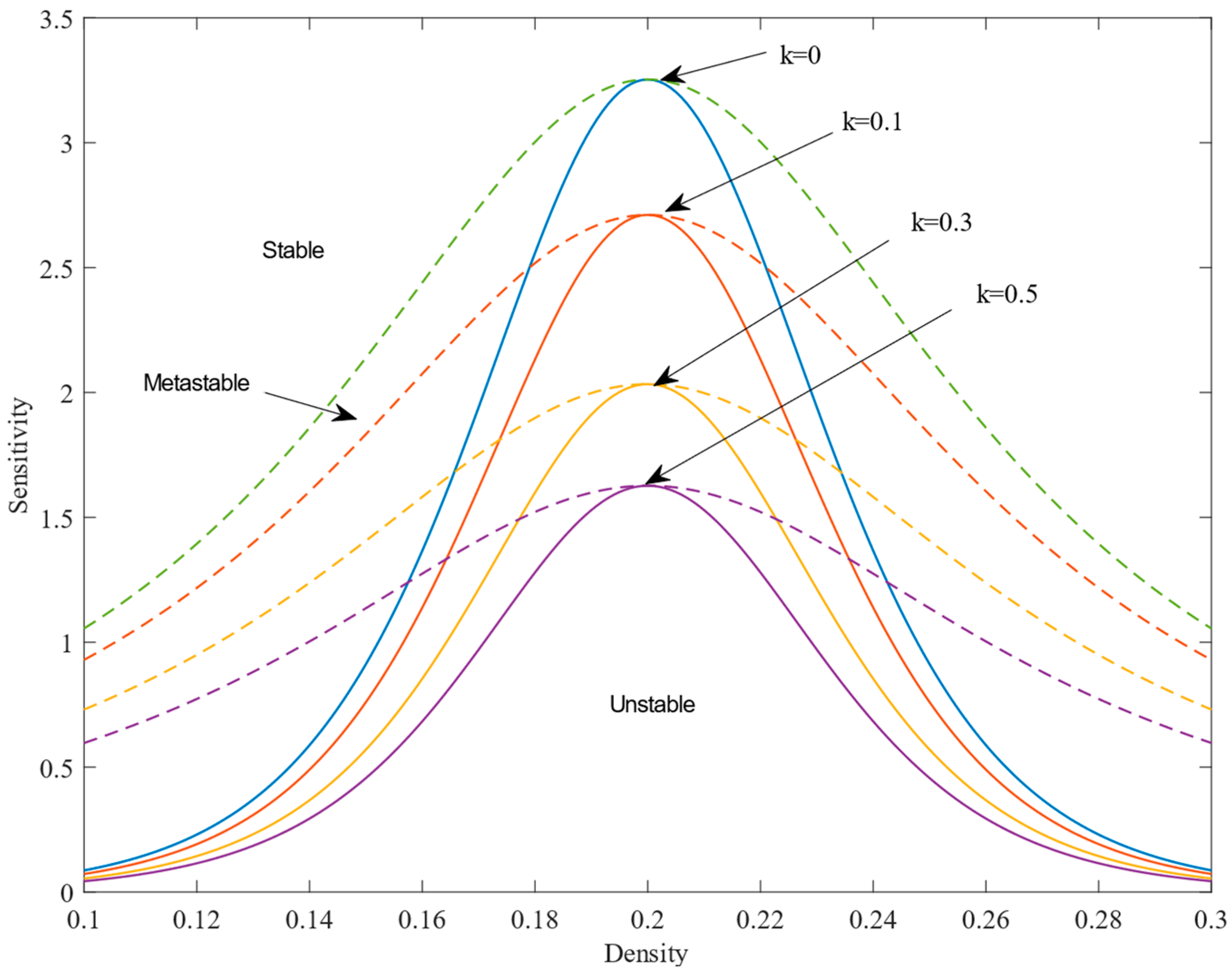
Figure 2 and Figure 3, respectively, present the density–sensitivity phase diagrams of the new model under different k values (k = 0, 0.1, 0.3, 0.5) and various road curvature ${\theta }_j$ values (${\theta }_j$= π/4, π/3, 5π/12, π/2). In these figures, dashed lines correspond to coexistence curves derived from mKdV equation solutions (see the nonlinear analysis in Section 4), while solid lines represent critical stability curves defined by Equation (17). Each pair of coexistence and critical stability curves shares a common vertex—the critical stability point, with coordinates $({\rho }_c,a_c)$—which divides the phase space into three regions: stable, metastable, and unstable. In the stable region, small disturbances do not intensify over time; traffic flow self-adjusts back to a stable state. Conversely, in the metastable and unstable regions, minor disturbances gradually amplify, triggering traffic congestion.

As observed in Figure 2, as the value of k increases, the position of the critical stability point gradually drops, and the stable region expands incrementally. This reflects an enhancement in both the stability and anti-interference capability of traffic flow on curved roads. Parameter k is used to quantify the feedback regulation intensity of flow difference information and has a significant impact on the response capability to small disturbances in traffic flow on curved roads. In practical applications, the reasonable value of parameter k should be calibrated by integrating the constraint range of stability condition (18) with field-measured data. In Figure 3 ($k=0.1$), it is evident that as the radian ${\theta }_j$ increases, the stability of traffic flow on the curved road continuously improves. Notably, when ${\theta }_j=\pi /2$ (corresponding to a straight road), the traffic flow stability reaches an optimal state, which aligns with practical traffic experiences. The aforementioned theoretical analysis sufficiently demonstrates that the radian of a curved road exerts a notable impact on the operational stability of traffic flow. Moreover, in curved road scenarios, leveraging flow difference information can effectively suppress the propagation and amplification of upstream disturbance signals, facilitating the formation of stable traffic flow.

4. Nonlinear Analysis

For curved road systems, when density exceeds ${\rho }_c$, traffic jams and nonlinear phenomena emerge. To study how flow differences affect spatiotemporal evolution near (${\rho }_c$, $a_c$), we apply nonlinear analysis. Near (${\rho }_c$, $a_c$), we define slow variables $X$ and $T$ for time t and space $j$ as follows:

$$X=\epsilon (j+bt),T={\epsilon }^{3}t,0<\epsilon \le 1$$

(20)

where $b$ is a parameter to be determined, let the density

$${\rho }_j(t)={\rho }_c+\epsilon R(X,T)$$

(21)

By substituting Equations (20) and (21) into Equation (10) and conducting a Taylor expansion up to the order of ${\epsilon }^5$ around the critical point $({\rho }_c,a_c)$, the resulting partial differential equation is

$$\begin{array}{l}{\epsilon }^2(b+{\displaystyle \frac{1}{{\sin }^2{\theta }_j}}{\rho }_c^2{V}^{\prime }){\mathsf{\partial }}_{X}R+{\epsilon }^3[{\displaystyle \frac{3}{2}}{b}^2\tau +{\displaystyle \frac{1}{2{\sin }^2{\theta }_j}}{\rho }_c^2{V}^{\prime }-kb]{\mathsf{\partial }}_X^{2}R\\ +{\epsilon }^4\{{\mathsf{\partial }}_{T}R+[{\displaystyle \frac{7b^3{\tau }^2}{6}}+{\displaystyle \frac{1}{6{\sin }^2{\theta }_j}}{\rho }_c^2{V}^{\prime }-{\displaystyle \frac{kb(b\tau +1)}{2}}]{\mathsf{\partial }}_X^{3}R+{\displaystyle \frac{{\rho }_c^2{V}^{‴}}{6{\sin }^2{\theta }_j}}{\mathsf{\partial }}_X{R}^3\}\\ +{\epsilon }^5\{(3b\tau -k){\mathsf{\partial }}_X{\mathsf{\partial }}_{T}R+[{\displaystyle \frac{5b^4{\tau }^3}{8}}+{\displaystyle \frac{1}{24{\sin }^2{\theta }_j}}{\rho }_c^2{V}^{\prime }\\ -{\displaystyle \frac{k}{24}}(4b^3{\tau }^2+6b^2\tau +4b)]{\mathsf{\partial }}_X^{4}R+{\displaystyle \frac{1}{12{\sin }^2{\theta }_j}}{\rho }_c^2{V}^{‴}{\mathsf{\partial }}_X^2{R}^3\}=0\end{array}$$

(22)

where $V^{’}=[{\displaystyle \frac{dV({\rho }_j)}{d{\rho }_j}}]|{\rho }_j={\rho }_c$ and $V^{‴}=[{\displaystyle \frac{d^{3}V({\rho }_j)}{d{\rho }_j^3}}]|{\rho }_j={\rho }_c$. At the critical point $({\rho }_c,a_c)$, let $\tau =(1+{\epsilon }^2){\tau }_c$, setting $b=-{\rho }_c^2{V}^{’}/{\mathit{sin}}^2{\theta }_j$, and eliminating the second-order and third-order $\epsilon$ terms in Equation (22), resulting in

$${\epsilon }^4[{\mathsf{\partial }}_{T}R-g_1{\mathsf{\partial }}_X^{3}R+g_2{\mathsf{\partial }}_X{R}^3]+{\epsilon }^5[g_3{\mathsf{\partial }}_X^{2}R+g_4{\mathsf{\partial }}_X^{4}R+g_5{\mathsf{\partial }}_X^2{R}^3]=0$$

(23)

where

$$g_1=-{\displaystyle \frac{7b^3{\tau }_c^2}{6}}-{\displaystyle \frac{1}{6{\sin }^2{\theta }_j}}{\rho }_c^2{V}^{\prime }+{\displaystyle \frac{1}{2}}kb(b{\tau }_c+1)$$

(24)

$$g_2={\displaystyle \frac{{\rho }_c^2{V}^{‴}}{6{\sin }^2{\theta }_j}}$$

(25)

$$g_3={\displaystyle \frac{3}{2}}{b}^2{\tau }_c$$

(26)

$$g_4=(3b{\tau }_c-k)g_1+{\displaystyle \frac{5}{8}}{b}^4{\tau }_c^3+{\displaystyle \frac{1}{24{\sin }^2{\theta }_j}}{\rho }_c^2{V}^{\prime }-{\displaystyle \frac{k}{24}}(4b^3{\tau }_c^2+6b^2{\tau }_c+4b),$$

(27)

$$g_5={\displaystyle \frac{1-6b{\tau }_c+2k}{12{\sin }^2{\theta }_j}}{\rho }_c^2{V}^{‴}$$

(28)

Through transforming Equation (23), we can derive the mKdV equation, which is as follows:

$$T^{\prime }=g_{1}T,R=\sqrt{{\displaystyle \frac{g_1}{g_2}}}{R}^{\prime }$$

(29)

Starting from Equation (29), the partial differential equation containing higher-order infinitesimal terms given below is derived:

$${\mathsf{\partial }}_{T^{\prime }}{R}^{\prime }-{\mathsf{\partial }}_X^3{R}^{\prime }+{\mathsf{\partial }}_X{R^{\prime }}^3+\epsilon M[R^{\prime }]=0$$

(30)

where

$$M[R^{\prime }]={\displaystyle \frac{1}{g_1}}[g_3{\mathsf{\partial }}_X^2{R}^{\prime }+g_4{\mathsf{\partial }}_X^4{R}^{\prime }+{\displaystyle \frac{g_1{g}_5}{g_2}}{\mathsf{\partial }}_X^2{R^{\prime }}^3]$$

(31)

Omitting the $O\left(\epsilon \right)$ terms in Equation (30), the kink–antikink solution of the standard mKdV equation is as follows:

$${R^{\prime }}_0(X,T^{\prime })=\sqrt{c}\tanh \sqrt{{\displaystyle \frac{c}{2}}}(X-c{T}^{\prime })$$

(32)

Drawing on reference [41], by integrating Equation (32), we can obtain the propagation velocity of the traffic density wave:

$$c={\displaystyle \frac{5g_2{g}_3}{2g_2{g}_4-3g_1{g}_5}}$$

(33)

Thus, taking into account the impact of flow difference in curved road situations, the kink–antikink density wave solution of the new model is

$${\rho }_j(t)={\rho }_c+\sqrt{{\displaystyle \frac{g_{1}c}{g_2}}({\displaystyle \frac{\tau }{{\tau }_c}}-1)}\tanh \sqrt{{\displaystyle \frac{c}{2}}({\displaystyle \frac{\tau }{{\tau }_c}}-1)}[j+(1-c{g}_1({\displaystyle \frac{\tau }{{\tau }_c}}-1))t]$$

(34)

The amplitude $A$ of the kink–antikink wave solution is

$$A=\sqrt{{\displaystyle \frac{g_{1}c}{g_2}}({\displaystyle \frac{\tau }{{\tau }_c}}-1)}$$

(35)

Nonlinear analysis shows the new model yields a kink–antikink wave solution. This solution describes coexisting phases: free flow (${\rho }_j={\rho }_c-A$, low density) and jammed flow (${\rho }_j={\rho }_c+A$, high density).

By examining Equations (24) and (26)–(28), it can be observed that the flow difference factor exerts an influence, via coefficient $k$, on $g_1$, $g_3$, $g_4$, $g_5$ and the propagation speed c of the density wave in Equation (33). This, in turn, acts on the density wave solution of the new model. When $k=0$, the new model proposed in this paper yields the mKdV equation and density wave solution consistent with Zhou’s model.

Table 1. Critical sensitivity a_c and density wave velocity c of the new model for different $k$ when ${\theta }_j=\pi /4$.

	k	0	0.05	0.1	0.15	0.2	0.25	0.3
The new model	ac	3.2533	2.9576	2.7111	2.5025	2.3238	2.1689	2.0333
	c	27	23.8832	21.7391	20.2323	19.1761	18.4615	18.0240

presents the distributions of critical sensitivity and density wave velocity for the new model under different values of $k$ when ${\theta }_j=\pi /4$. When $k=0$, the new model degenerates into the model proposed by Zhou et al. Due to the introduction of the flow difference factor, the critical sensitivity coefficient of drivers and the propagation velocity of density waves in the new model are significantly lower than those in Zhou’s model. Moreover, both the critical sensitivity and the velocity of density waves in the new model decrease with the increase in $k$. This indicates that the flow difference factor has a damping effect similar to that in reference [42], and its introduction can enhance the stability of curved traffic flow, with the stability improving as $k$ increases.

Table 2. Critical sensitivity a_c and density wave velocity c of the new model and Zhou’s model under different ${\theta }_j$.

	${\mathit{\theta }}_{\mathit{j}}$	$\mathit{\pi }/6$	$\mathit{\pi }/4$	$\mathit{\pi }/3$	$5\mathit{\pi }/12$	$\mathit{\pi }/2$
The new model	ac	5.4222	2.7111	1.8074	1.4529	1.3555
	c	21.7391	21.7391	21.7391	21.7391	21.7391
Zhou’s model	ac	6.5066	3.2533	2.1689	1.7434	1.6267
	c	27.0000	27.0000	27.0000	27.0000	27.0000

shows the distributions of critical sensitivity and density wave velocity for the new model proposed in this paper ($k=0.1$) and Zhou’s model under different ${\theta }_j$, respectively. Under the same conditions, the values of critical sensitivity and density wave in our model are significantly lower than those in Zhou’s model. The sensitivity coefficient and density wave velocity are reduced by approximately 16.67% and 19.48%, respectively, compared with Zhou’s model. This demonstrates that our model has stronger stability and traffic congestion suppression ability, and its stability is enhanced as ${\theta }_j$ increases.

To further illustrate the improvement effect of the new model, a comparison is made with the classic curve lattice model proposed by Cao et al. [25].

Table 3. Critical sensitivity a_c and density wave velocity c of the new model and Cao’s model under different $R$.

	$\mathit{R}$	$30$	$60$	$90$	$120$	150	$180$
The new model	ac	1.6602	2.3479	2.8755	3.3204	3.7123	4.0666
	c	21.7391	21.7391	21.7391	21.7391	21.7391	21.7391
Cao’s model	ac	1.9922	2.8174	3.4507	3.9845	4.4548	4.8800
	c	27.0000	27.0000	27.0000	27.0000	27.0000	27.0000

presents the distribution of density wave propagation speed and critical sensitivity in both the proposed model ($k=0.1$) and Cao’s model under different curve radii. The results show that under the same curve radius, due to the introduction of the flow difference effect, both the critical sensitivity coefficient and the density wave propagation speed of the proposed model are lower than those of Cao’s model. This indicates that the flow difference effect has a positive stabilizing effect on curved traffic flow.

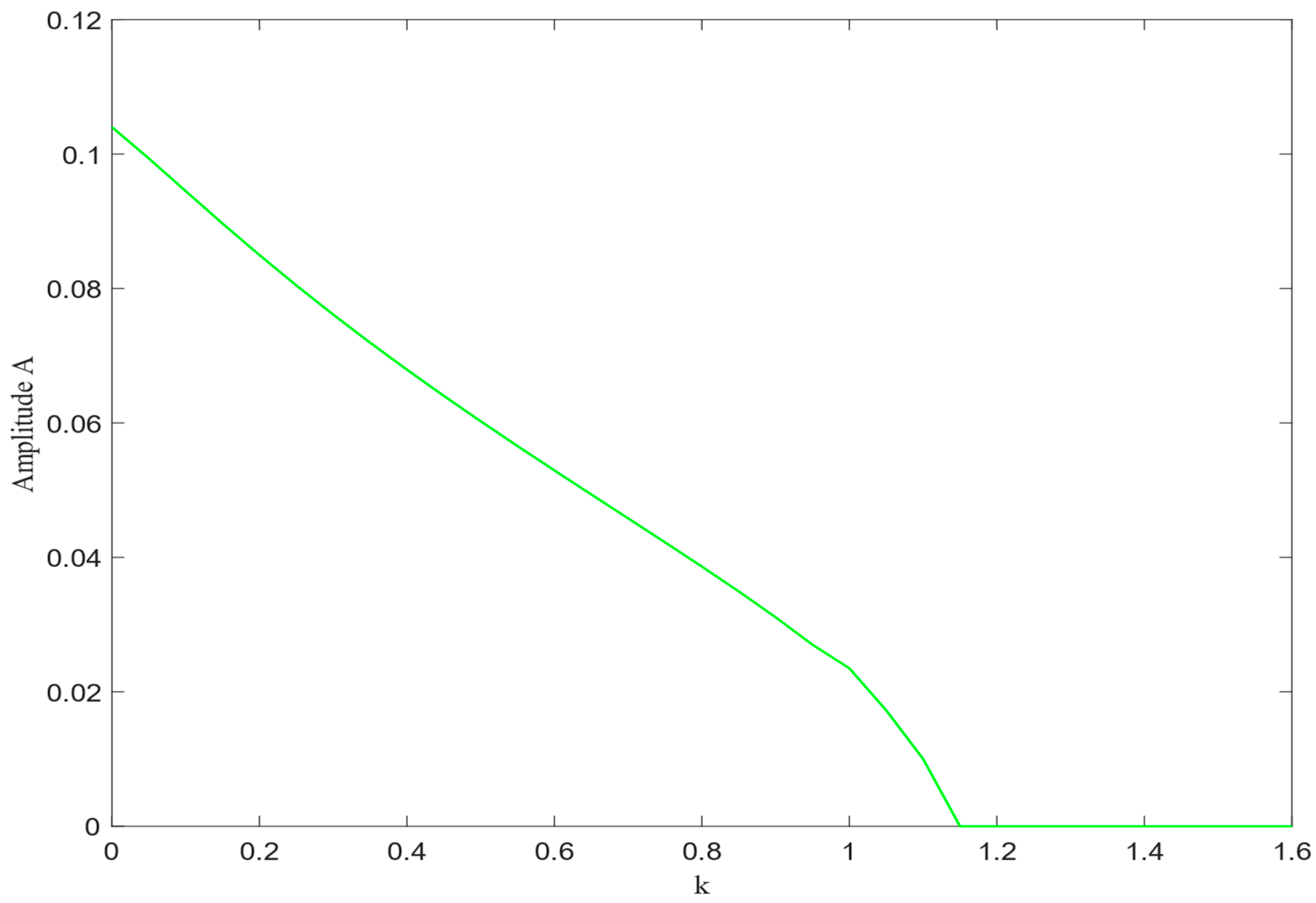
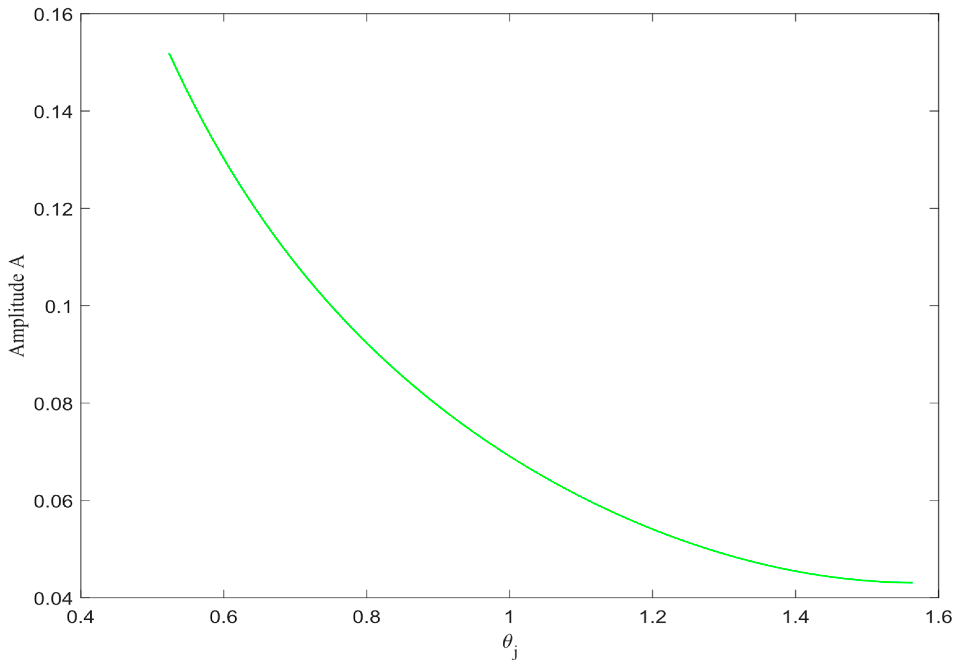
According to Equation (35), when $\tau =1$, Figure 4 and Figure 5 respectively illustrate the variation patterns of the density wave amplitude A with parameters $k$ and ${\theta }_j$ in the proposed model. It can be observed that as $k$ and ${\theta }_j$ increase, the density wave amplitude gradually decreases, traffic congestion is progressively mitigated, and the traffic flow stability is incrementally enhanced.

5. Numerical Simulation

To validate the theoretical analysis, numerical simulations under periodic boundaries use density evolution Equation (10) for curved roads. Initial conditions are

$${\rho }_j(0)={\rho }_j(1)=\left\{\begin{array}{c}{\rho }_0-A; 0\le j<{\displaystyle \frac{N}{2}}\\ {\rho }_0+A; {\displaystyle \frac{N}{2}}\le j<N\end{array}\right.$$

(36)

where the total number of grids in the simulated system is $N=100$, ${\rho }_0={\rho }_c=0.2$, and the initial perturbation is $A=0.05$. The other simulation input parameters are as follows: $g=10$, $\mu =0.3$, $R=20$, and $\beta =0.14$. For better clarity and readability, we have provided a summary of the key parameters employed in the simulation model, with specific information outlined in

Table 4. The query table of main parameters.

Notation	Definition	Value	UNIT
N	The number of grid cells in the simulation	100	-
j	The numbering of road segments.		-
a	driver sensitivity coefficient.		s−1
t	Time		s
$\tau$	Driver’s reaction time delay, $\tau =1/a$.		s
${\rho }_0$	The total average density of traffic system.	0.2	veh/km
${\rho }_c$	Critical density.	0.2	veh/km
$g$	The gravity acceleration.	10	m/s2
$\mu$	Road-surface friction coefficient.	0.3	-
$\beta$	Control coefficient.	0.14	-
R	The road’s radius of curvature.	20	km
${\theta }_j$	The radian corresponding to the $j$-th lattice point.		rad
k	traffic flow difference response intensity coefficient.		s−1
V	Optimized velocity function.		km/h
$v_j(t)$	The average speed of road segment j at time t.		km/h
${\rho }_j(t)$	The average density of road segment j at time t.		veh/km

. The simulation results are shown in Figure 6, Figure 7, Figure 8, Figure 9, Figure 10 and Figure 11.

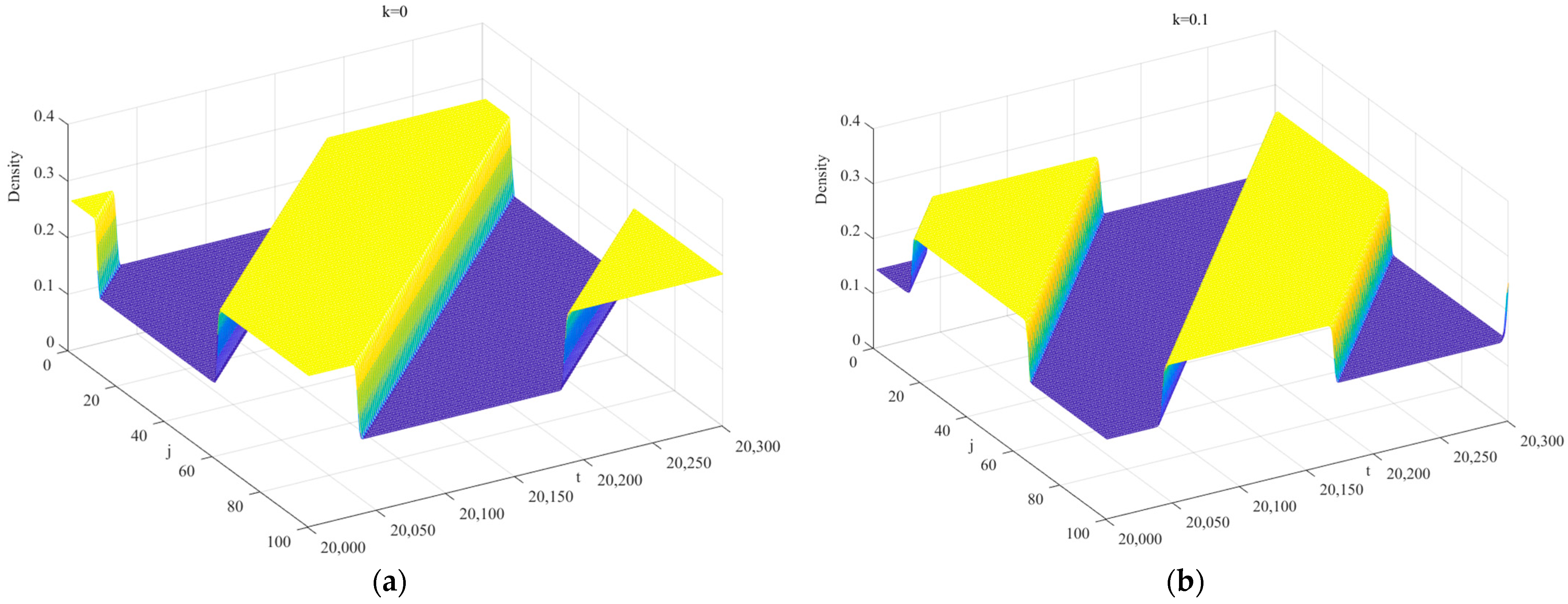
Figure 6a–d present three-dimensional traffic density images of the novel model after t = 20,000, with $k=0, 0.1, 0.3, 0.5$, $a=1.8$, and ${\theta }_j=\pi /4$. Increasing k reduces density fluctuations, enhancing curved road traffic stability. Notably, when $k=0$ (Figure 6a), the model degenerates to Zhou and Shi’s curved lattice model [26]. In Figure 6a–c, stability condition (18) is violated: small perturbations propagate and amplify, triggering stop-and-go traffic jams. At k = 0.5, condition (18) holds: disturbances decay during propagation, and traffic returns to free flow (see Figure 6d).

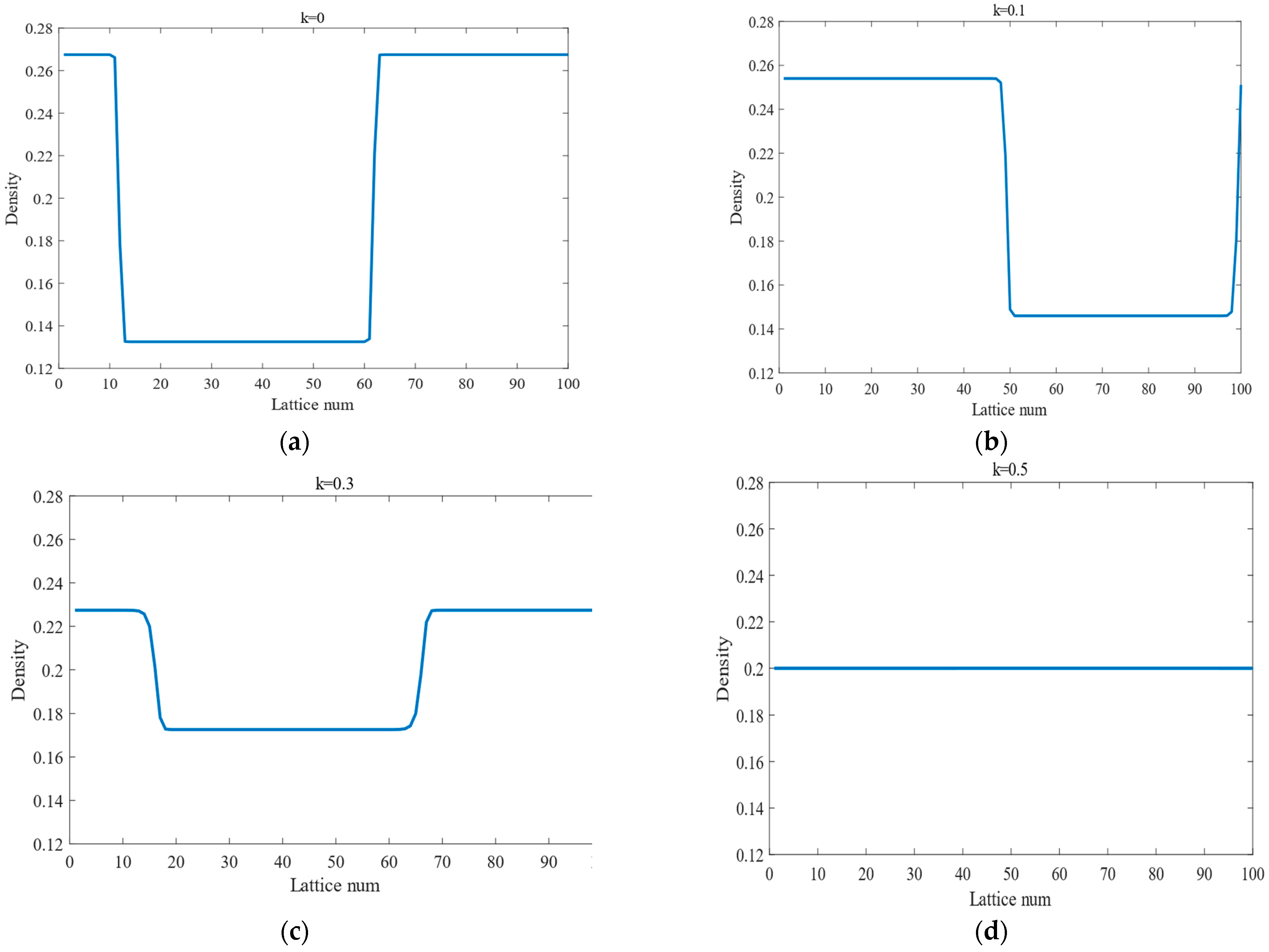
Figure 7 (corresponding to Figure 6) depicts the traffic density distribution at t = 20,300. In curved road scenarios, unstable traffic propagates as kink-antikink density waves (governed by the mKdV equation). Under the same sensitivity and initial density, increasing k gradually decays the density wave amplitude (traffic jams), significantly alleviating congestion.

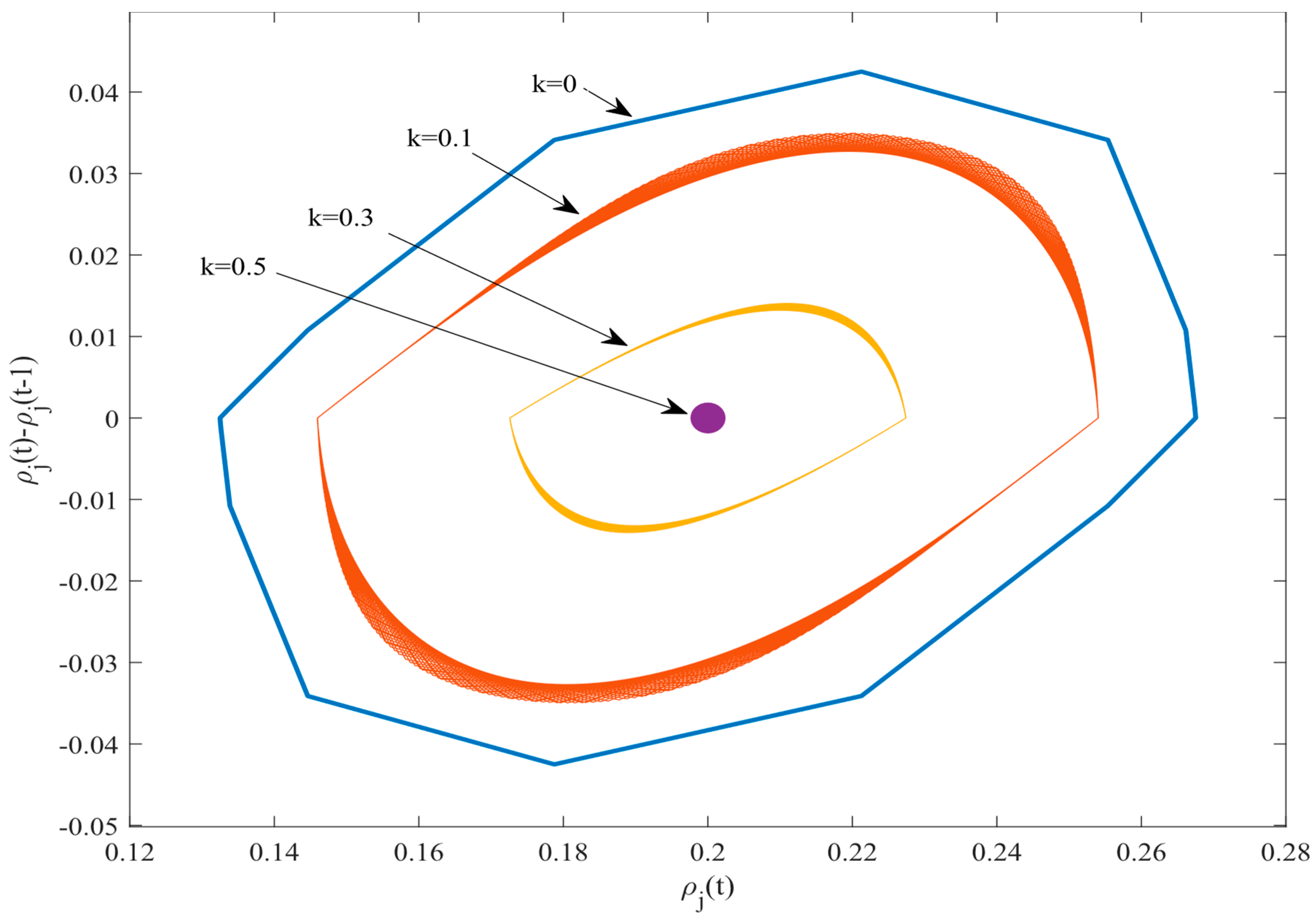
To more intuitively illustrate the influence of the flow difference factor on the stability of the curved road traffic system, Figure 8 presents the relationship between the density difference ${\rho }_j(t)-{\rho }_j(t-1)$ and the density ${\rho }_j(t)$ in the new model under different values of parameter k within the time interval t = 15,000−20,300. The trajectory of the dataset (${\rho }_j(t)-{\rho }_j(t-1)$, ${\rho }_j(t)$) forms a hysteresis loop, and the area of the loop reflects the stability of traffic operation (the smaller the area, the more stable the traffic). As can be seen from Figure 8, as the parameter k increases, the area of the hysteresis loop gradually decreases. Notably, when k = 0.5, the hysteresis loop degenerates into a point, which means that the traffic flow reaches a stable state.

From the simulation results shown in Figure 6, Figure 7 and Figure 8, it is inferred that the flow difference effect plays a remarkably significant stabilizing role in curved road environments. It effectively mitigates traffic congestion. Thus, integrating the flow difference factor into the current curved lattice model framework is of substantial practical importance.

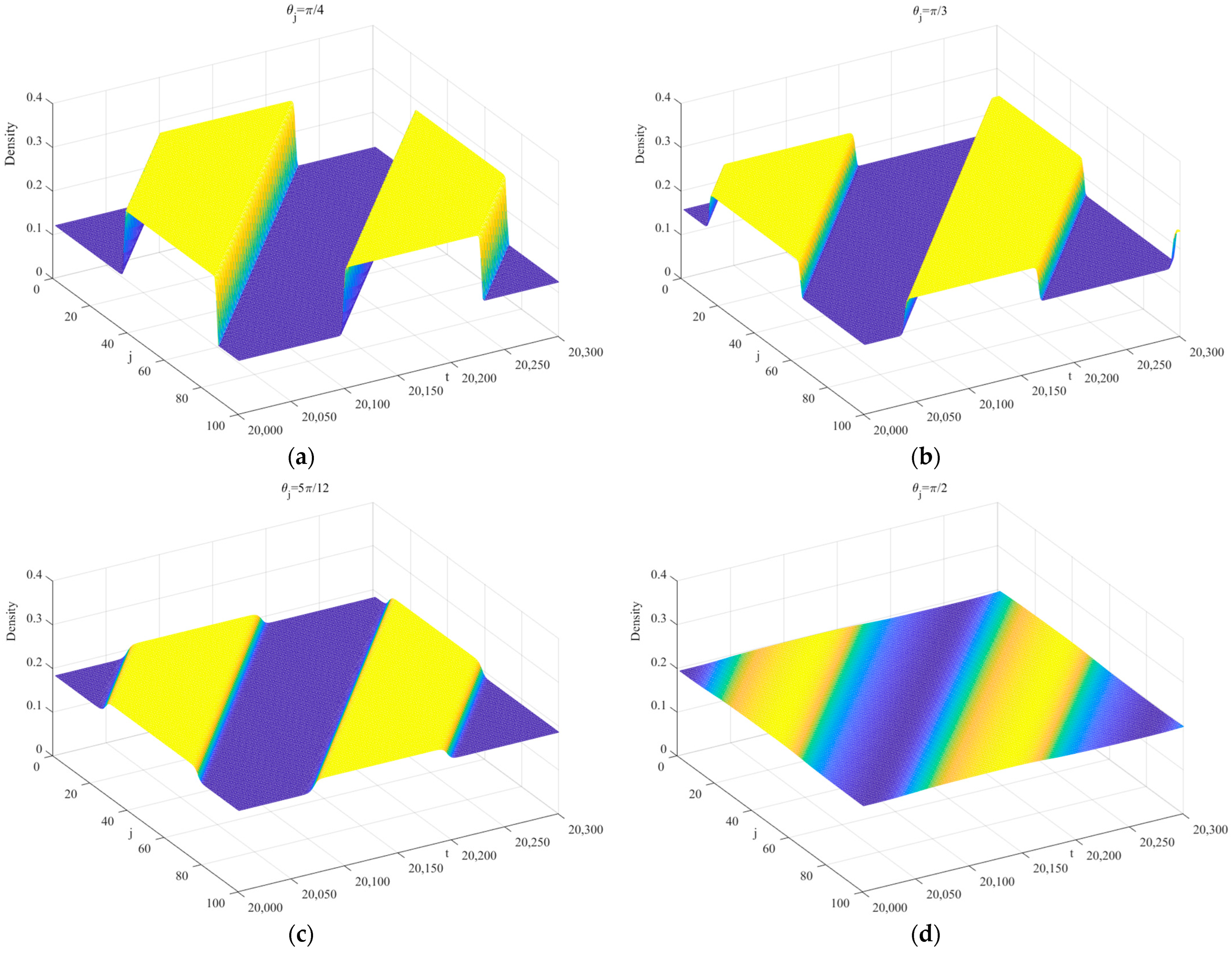
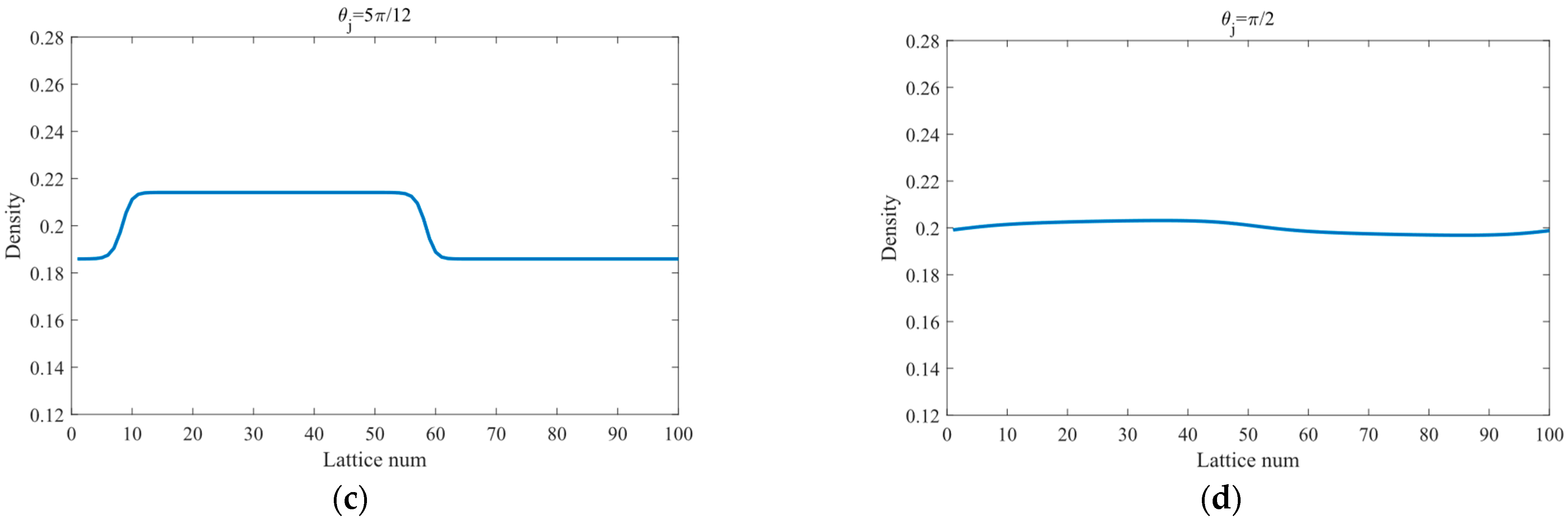
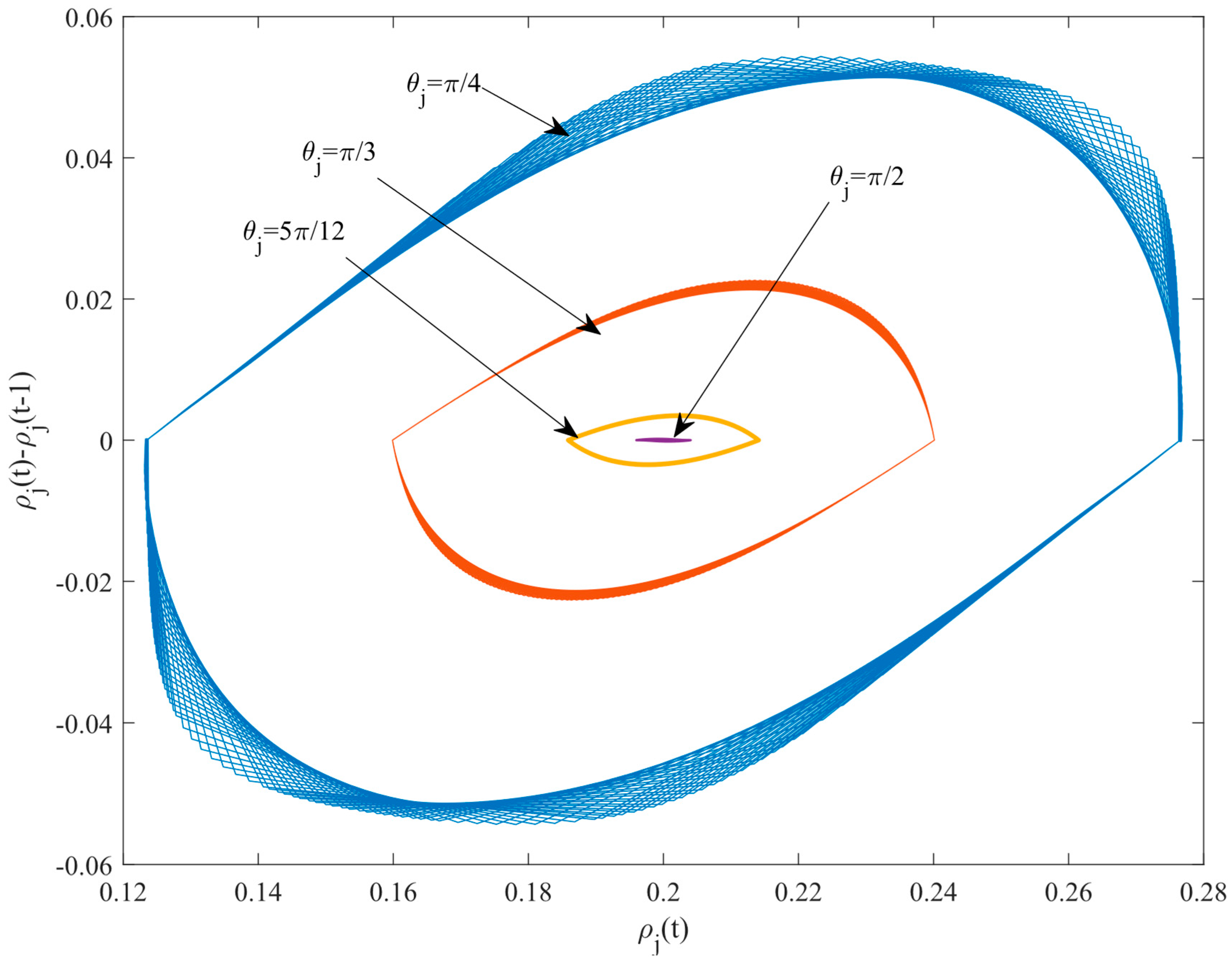
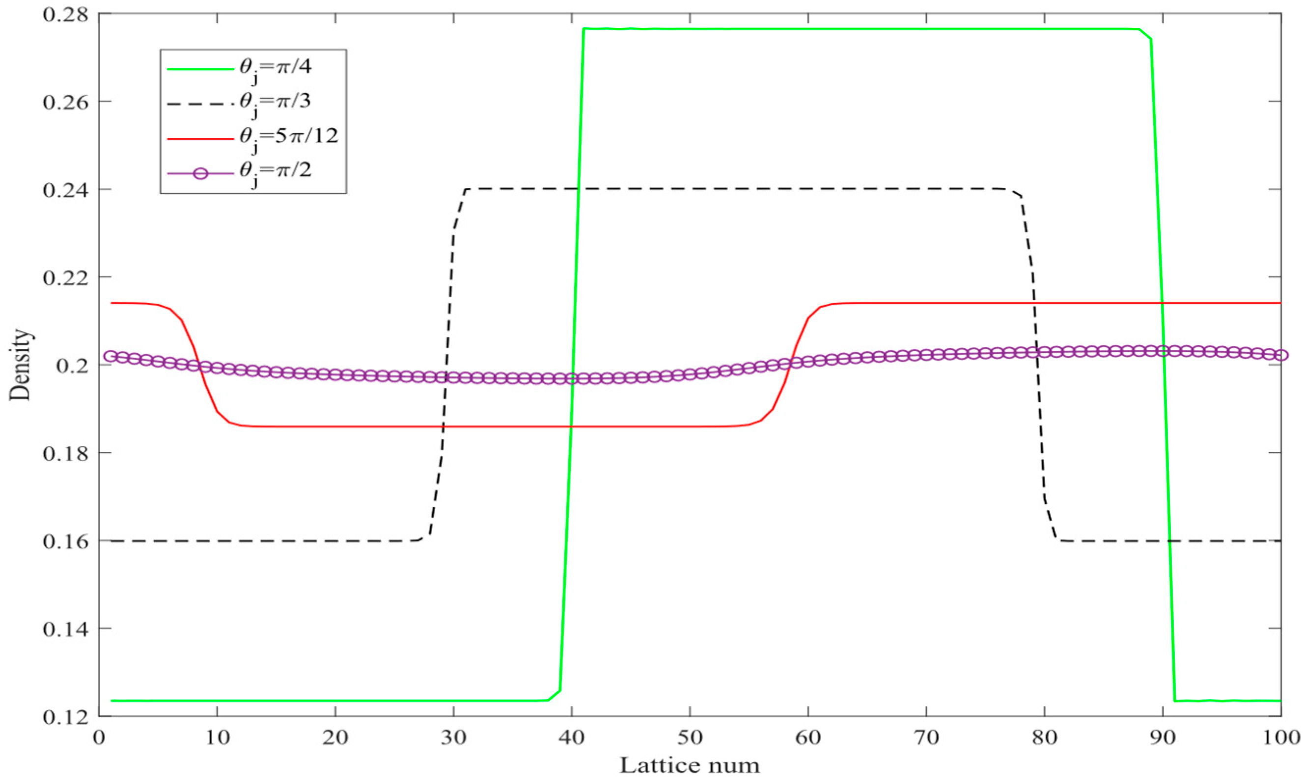
Figure 9a–d depict the spatiotemporal evolution of traffic density at time step t = 20,000 for different ${\theta }_j$ values ($\pi /4,\pi /3,5\pi /12,\pi /2$) under input parameters $a=1.4$ and $k=0.1$. Figure 10 illustrates the traffic density distribution across all lattice points corresponding to Figure 9 at t = 20,300. As shown in Figure 9 and Figure 10, when ${\theta }_j$ takes values of $\pi /4$, $\pi /3$, and $5\pi /12$ (Figure 9a–c and Figure 10a–c), the stability condition (18) is violated, leading to the amplification of disturbance signals over time and causing stop-and-go traffic congestion. Notably, under the same sensitivity conditions, a larger ${\theta }_j$ results in a smaller fluctuation amplitude of density waves and smoother traffic flow operation. Specifically, when ${\theta }_j=\pi /2$ (horizontal straight road), the stability condition (18) is satisfied, and small disturbance signals are completely absorbed over time, restoring the traffic flow to a stable free-flow state (Figure 9d and Figure 10d). Additionally, Figure 11 shows the hysteresis loops for different ${\theta }_j$ values in the new model during the time steps 15,000−20,300. It is observed that the area of the hysteresis loop gradually decreases with increasing ${\theta }_j$, indicating a continuous improvement in traffic flow stability.

Thus, based on the simulation outcomes depicted in Figure 9, Figure 10 and Figure 11, the following inference can be made: The curvature of the curved roadway exerts a substantial influence on traffic flow stability. Specifically, traffic stability demonstrates a gradual enhancement as roadway curvature increases, a finding that aligns with both the stability analysis results and real-world observations.

To verify whether the above simulation results depend on the perturbation intensity in Equation (36), we conducted a numerical analysis under a new perturbation scale, where the initial perturbation $A$ is set to 0.1 while all other input parameters remain unchanged. Figure 12 and Figure 13 present the traffic density distributions at t = 20,300 corresponding to different values of k and ${\theta }_j$, respectively. The results in Figure 12 and Figure 13 indicate that the stability of traffic flow gradually improves as the parameters k or ${\theta }_j$ gradually increase. This conclusion is consistent with that obtained under the conditions of Equation (36), thus demonstrating that the simulation conclusions are general and independent of the initial perturbation scale.

6. Conclusions

To address the issue of traffic flow modeling on curved roads, this study proposes an improved lattice hydrodynamic model that integrates the geometric characteristics of curves and traffic flow difference information. The key conclusions derived from theoretical analysis and numerical simulations are as follows:

(1) Based on lattice hydrodynamic theory, the new model effectively incorporates the combined effects of curve geometric features and traffic flow differences on macroscopic traffic flow. Its stability criterion is derived using linear stability theory. Meanwhile, through nonlinear analysis, the mKdV equation describing the propagation law of traffic congestion near the critical point is successfully deduced, along with its density wave solution.

(2) Both theoretical and simulation results indicate that the stability of traffic flow increases significantly with the growth of curve curvature. Additionally, the introduction of the traffic flow difference factor can effectively suppress the accumulation and propagation of traffic waves and reduce drivers’ critical sensitivity.

(3) Compared with the classical model by Zhou et al., the new model exhibits a reduction of approximately 16.67% in critical sensitivity and 19.48% in density wave propagation speed, demonstrating superior congestion mitigation performance. These findings provide a theoretical reference for the optimal control of traffic flow on curved roads.

However, the proposed model has only been subjected to theoretical analysis and numerical simulation and lacks comparison with field measurement results of actual traffic. In the future, to verify the model’s practicality and rationality, we plan to collect field-measured data to calibrate the model. Furthermore, with the accumulation of massive sensing data in the transportation domain, we can draw on the ideas and technical framework of References [43,44] to break free from the reliance of traditional traffic flow models on empirical assumptions and explore data-driven approaches to traffic flow modeling.

References

1. Liu, K.; Feng, T. Heterogeneous traffic flow cellular automata model mixed with intelligent controlled vehicles. Phys. A Stat. Mech. Its Appl. 2023, 632, 129316. [Google Scholar] [CrossRef]
2. Fukui, M.; Ishibashi, Y. Traffic flow in 1d cellular automaton model including cars moving with high speed. J. Phys. Soc. Jpn. 1996, 65, 1868–1870. [Google Scholar] [CrossRef]
3. Zhai, C.; Wu, W.; Xiao, Y. Cooperative car-following control with electronic throttle and perceived headway errors on gyroidal roads. Appl. Math. Model. 2022, 108, 770–786. [Google Scholar] [CrossRef]
4. Sun, Y.; Ge, H.; Cheng, R. A car-following model considering the effect of electronic throttle opening angle over the curved road. Phys. A Stat. Mech. Its Appl. 2019, 534, 122377. [Google Scholar] [CrossRef]
5. Zhai, C.; Wu, W. A continuous traffic flow model considering predictive headway variation and preceding vehicle’s taillight effect. Phys. A Stat. Mech. Its Appl. 2021, 584, 126364. [Google Scholar] [CrossRef]
6. Jiang, R.; Wu, Q.-S.; Zhu, Z.-J. A new continuum model for traffic flow and numerical tests. Transp. Res. Part B Methodol. 2002, 36, 405–419. [Google Scholar] [CrossRef]
7. Nagatani, T. Modified KdV equation for jamming transition in the continuum models of traffic. Phys. A Stat. Mech. Its Appl. 1998, 261, 599–607. [Google Scholar] [CrossRef]
8. Nagatani, T. Jamming transitions and the modified Korteweg–de Vries equation in a two-lane traffic flow. Phys. A Stat. Mech. Its Appl. 1999, 265, 297–310. [Google Scholar] [CrossRef]
9. Wang, T.; Zang, R.; Xu, K.; Zhang, J. Analysis of predictive effect on lattice hydrodynamic traffic flow model. Phys. A Stat. Mech. Its Appl. 2019, 526, 120711. [Google Scholar] [CrossRef]
10. Kaur, D.; Sharma, S. A new two-lane lattice model by considering predictive effect in traffic flow. Phys. A Stat. Mech. Its Appl. 2020, 539, 122913. [Google Scholar] [CrossRef]
11. Kang, Y.-R.; Tian, C. A new curved road lattice model integrating the multiple prediction effect under V2X environment. Phys. A Stat. Mech. Its Appl. 2024, 643, 129812. [Google Scholar] [CrossRef]
12. Zhai, C.; Wu, W.; Xiao, Y. An extended multi-lane lattice hydrodynamic model considering the predictive effect of drivers under connected vehicle environment. J. Transp. Eng. Part A Syst. 2023, 149, 04023099. [Google Scholar] [CrossRef]
13. Redhu, P.; Siwach, V. An extended lattice model accounting for traffic jerk. Phys. A Stat. Mech. Its Appl. 2018, 492, 1473–1480. [Google Scholar] [CrossRef]
14. Wang, T.; Cheng, R.; Ge, H. An extended two-lane lattice hydrodynamic model for traffic flow on curved road with passing. Phys. A Stat. Mech. Its Appl. 2019, 533, 121915. [Google Scholar] [CrossRef]
15. Jin, Y.-D.; Zhou, J.; Shi, Z.-K.; Zhang, H.-L.; Wang, C.-P. Lattice hydrodynamic model for traffic flow on curved road with passing. Nonlinear Dyn. 2017, 89, 107–124. [Google Scholar] [CrossRef]
16. Zhai, C.; Wu, W.; Xiao, Y. The jamming transition of multi-lane lattice hydrodynamic model with passing effect. Chaos Solitons Fractals 2023, 171, 113515. [Google Scholar] [CrossRef]
17. Peng, G.; Kuang, H.; Zhao, H.; Li, Q. Nonlinear analysis of a new lattice hydrodynamic model with the consideration of honk effect on flux for two-lane highway. Phys. A Stat. Mech. Its Appl. 2019, 515, 93–101. [Google Scholar] [CrossRef]
18. Peng, G.; Kuang, H.; Bai, K. The impact of the individual difference on traffic flow under honk environment in lattice hydrodynamic model. Phys. A Stat. Mech. Its Appl. 2019, 526, 120772. [Google Scholar] [CrossRef]
19. Mei, Y.; Zhao, X.; Qian, Y.; Xu, S.; Li, Z. Effect of self-stabilizing control in lattice hydrodynamic model with on-ramp and off-ramp. Phys. A Stat. Mech. Its Appl. 2021, 575, 126048. [Google Scholar] [CrossRef]
20. Zhang, G.; Sun, D.-H.; Zhao, M. Phase transition of a new lattice hydrodynamic model with consideration of on-ramp and off-ramp. Commun. Nonlinear Sci. Numer. Simul. 2018, 54, 347–355. [Google Scholar] [CrossRef]
21. Jiang, C.; Cheng, R.; Ge, H. Mean-field flow difference model with consideration of on-ramp and off-ramp. Phys. A Stat. Mech. Its Appl. 2019, 513, 465–476. [Google Scholar] [CrossRef]
22. Tian, C.; Kang, Y. Modeling and optimal congestion control of multi-lane highway traffic with on-ramp and off-ramp under V2X environment. Phys. A Stat. Mech. Its Appl. 2025, 661, 130409. [Google Scholar] [CrossRef]
23. Peng, G.; Zhao, H.; Li, X. The impact of self-stabilization on traffic stability considering the current lattice’s historic flux for two-lane freeway. Phys. A Stat. Mech. Its Appl. 2019, 515, 31–37. [Google Scholar] [CrossRef]
24. Zhang, G. The self-stabilization effect of lattice’s historical flow in a new lattice hydrodynamic model. Nonlinear Dyn. 2018, 91, 809–817. [Google Scholar] [CrossRef]
25. Cao, J.-L.; Shi, Z.-K. A novel lattice traffic flow model on a curved road. Int. J. Mod. Phys. C 2015, 26, 1550121. [Google Scholar] [CrossRef]
26. Zhou, J.; Shi, Z.-K. Lattice hydrodynamic model for traffic flow on curved road. Nonlinear Dyn. 2016, 83, 1217–1236. [Google Scholar] [CrossRef]
27. Zhou, J.; Shi, Z.-K.; Wang, C.-P. Lattice hydrodynamic model for two-lane traffic flow on curved road. Nonlinear Dyn. 2016, 85, 1423–1443. [Google Scholar] [CrossRef]
28. Xiao, Y.; Wu, W.; Zhai, C.; Zhai, M.; Zhang, J. Analysis of empirical lane-changing rate effect on multi-lane traffic on curved roads. Chin. J. Phys. 2025, 95, 260–274. [Google Scholar] [CrossRef]
29. Wang, Q.; Cheng, R.; Ge, H. A novel lattice hydrodynamic model accounting for driver’s memory effect and the difference of optimal velocity on curved road. Phys. A Stat. Mech. Its Appl. 2020, 559, 125023. [Google Scholar] [CrossRef]
30. Cheng, R.; Wang, Y. An extended lattice hydrodynamic model considering the delayed feedback control on a curved road. Phys. A Stat. Mech. Its Appl. 2019, 513, 510–517. [Google Scholar] [CrossRef]
31. Mehta, S.; Dangi, R.; Siwach, V.; Redhu, P. Effect of weather’s visibility on traffic dynamics: A novel lattice hydrodynamic model for curved roads with passing. Eur. Phys. J. B 2025, 98, 2. [Google Scholar] [CrossRef]
32. Wang, Y.; Zhang, C.; Zhu, C.; Hou, H.; Wang, Z. Analysis of traffic characteristics in mixed road environments based on a unified lattice hydrodynamic model. Eur. Phys. J. B 2025, 98, 134. [Google Scholar] [CrossRef]
33. Chang, Y.; Cheng, R. Effect of speed deviation and anticipation effect of flux difference in the lattice hydrodynamic model. Phys. A Stat. Mech. Its Appl. 2019, 531, 121751. [Google Scholar] [CrossRef]
34. Qin, S.; He, Z.; Cheng, R. An extended lattice hydrodynamic model based on control theory considering the memory effect of flux difference. Phys. A Stat. Mech. Its Appl. 2018, 509, 809–816. [Google Scholar] [CrossRef]
35. Wang, T.; Gao, Z.-Y.; Zhao, X.-M.; Tian, J.-F.; Zhang, W.-Y. Flow difference effect in the two-lane lattice hydrodynamic model. Chin. Phys. B 2012, 21, 070507. [Google Scholar] [CrossRef]
36. Tian, J.-F.; Jia, B.; Li, X.-G.; Gao, Z.-Y. Flow difference effect in the lattice hydrodynamic model. Chin. Phys. B 2010, 19, 040303. [Google Scholar] [CrossRef]
37. Jin, Y.; Meng, J.; Xu, M. Dynamical analysis for a car-following model with delayed-feedback control of both velocity and acceleration differences. Commun. Nonlinear Sci. Numer. Simul. 2022, 111, 106458. [Google Scholar] [CrossRef]
38. Li, S.; Cheng, R.; Ge, H. An improved car-following model considering electronic throttle dynamics and delayed velocity difference. Phys. A Stat. Mech. Its Appl. 2020, 558, 125015. [Google Scholar] [CrossRef]
39. Nagatani, T. Jamming transition in a two-dimensional traffic flow model. Phys. Rev. E 1999, 59, 4857. [Google Scholar] [CrossRef] [PubMed]
40. Al-Yaari, A.; Ching, D.L.C.; Sakidin, H.; Muthuvalu, M.S.; Zafar, M.; Alyousifi, Y.; Saeed, A.A.H.; Bilad, M.R. Thermophysical Properties of Nanofluid in Two-Phase Fluid Flow through a Porous Rectangular Medium for Enhanced Oil Recovery. Nanomaterials 2022, 12, 1011. [Google Scholar] [CrossRef] [PubMed]
41. Ge, H.X.; Cheng, R.J.; Dai, S.Q. KdV and kink-antikink solitons in car-following models. Phys. A Stat. Mech. Its Appl. 2005, 357, 466–476. [Google Scholar] [CrossRef]
42. Al-Yaari, A.; Ching, D.L.C.; Sakidin, H.; Muthuvalu, M.S.; Zafar, M.; Haruna, A.; Merican, Z.M.A.; Yunus, R.B.; Al-dhawi, B.N.S.; Jagaba, A.H. The effects of nanofluid thermophysical properties on enhanced oil recovery in a heterogenous porous media. Case Stud. Chem. Environ. Eng. 2024, 9, 100556. [Google Scholar] [CrossRef]
43. Liu, X.; Qiu, L.; Fang, Y.; Wang, K.; Li, Y.; Rodríguez, J. Event-Driven Based Reinforcement Learning Predictive Controller Design for Three-Phase NPC Converters Using Online Approximators. IEEE Trans. Power Electron. 2025, 40, 4914–4926. [Google Scholar] [CrossRef]
44. Chen, X.; Wu, S.; Shi, C.; Huang, Y.; Yang, Y.; Ke, R. Sensing Data Supported Traffic Flow Prediction via Denoising Schemes and ANN: A Comparison. IEEE Sens. J. 2020, 20, 14317–14328. [Google Scholar] [CrossRef]
Figure 1. The physical form of the model for a curved road.
Symmetry 17 01299 g001
Figure 2. Phase diagram for presented model in density-sensitivity space with different k when θ j = π / 4 .
Symmetry 17 01299 g002
Figure 3. Phase diagram for presented model in density-sensitivity space with different θ j when k = 0.1 .
Symmetry 17 01299 g003
Figure 4. The relationship between the density wave amplitude A and the parameter k in the proposed model when τ = 1 .
Symmetry 17 01299 g004
Figure 5. The relationship between the density wave amplitude A and the parameter θ j in the proposed model when τ = 1 .
Symmetry 17 01299 g005
Figure 6. Space-time evolution of the density after t = 20,000 for presented model (a) k = 0 , (b) k = 0.1 , (c) k = 0.3 , and (d) k = 0.5 when a = 1.8 and θ j = π / 4 .
Symmetry 17 01299 g006aSymmetry 17 01299 g006b
Figure 7. Density profiles at t = 20,300 for presented model (a) k = 0 , (b) k = 0.1 , (c) k = 0.3 , and (d) k = 0.5 when a = 1.8 and θ j = π / 4 .
Symmetry 17 01299 g007
Figure 8. Plot of the density difference ρ j ( t ) ρ j ( t 1 ) against density ρ j ( t ) for t = 15,000−20,300 when a = 1.8 and θ j = π / 4 for k = 0 , 0.1 , 0.3 , and 0.5, respectively. The smaller the area of the hysteresis loop in the figure, the stronger the stability.
Symmetry 17 01299 g008
Figure 9. Space−time evolution of the density after t = 20,000 for presented model (a) θ j = π / 4 , (b) θ j = π / 3 , (c) θ j = 5 π / 12 , and (d) θ j = π / 2 when a = 1.4 and k = 0.1 .
Symmetry 17 01299 g009
Figure 10. Density profiles at t = 20,300 for presented model (a) θ j = π / 4 , (b) θ j = π / 3 , (c) θ j = 5 π / 12 , and (d) θ j = π / 2 when a = 1.4 and k = 0.1 .
Symmetry 17 01299 g010aSymmetry 17 01299 g010b
Figure 11. Plot of the density difference ρ j ( t ) ρ j ( t 1 ) against density ρ j ( t ) for t = 15,000−20,300 when a = 1.4 , k = 0.1 for θ j = π / 3 , π / 4 , 5 π / 12 , and π / 2 , respectively. The smaller the area of the hysteresis loop in the figure, the stronger the stability.
Symmetry 17 01299 g011
Figure 12. Density profiles at time t = 20,300 with different value k when a = 1.8 and θ j = π / 4 .
Symmetry 17 01299 g012
Figure 13. Density profiles at time t = 20,300 with different value θ j when a = 1.4 and k = 0.1 .
Symmetry 17 01299 g013