Article

Multi-Scale Pure Graphs with Multi-View Subspace Clustering for Salient Object Detection

1
School of Earth Science and Engineering, Xi’an Shiyou University, Xi’an 710065, China
2
Shaanxi Key Laboratory of Petroleum Accumulation Geology, Xi’an Shiyou University, Xi’an 710065, China
3
College of Petroleum Engineering, Xi’an Shiyou University, Xi’an 710065, China
4
School of Science, Xi’an Shiyou University, Xi’an 710065, China
*
Author to whom correspondence should be addressed.
Symmetry 2025, 17(8), 1262; https://doi.org/10.3390/sym17081262
Submission received: 30 June 2025 / Revised: 21 July 2025 / Accepted: 1 August 2025 / Published: 7 August 2025
(This article belongs to the Section Engineering and Materials)

Abstract

Salient object detection is a challenging task in the field of computer vision. The graph-based model has attracted lots of research attention and achieved remarkable progress in this task, which constructs graphs to formulate the intrinsic structure of any image. Nevertheless, the existing graph-based salient object detection methods still have certain limitations and face two major challenges: (1) Previous graphs are constructed by the Gaussian kernel, but they are often corrupted by original noise. (2) They fail to capture common representations and complementary diversity of multi-view features. Both of these degrade saliency performance. In this paper, we propose a novel method, called multi-scale pure graphs with multi-view subspace clustering for salient object detection. Its main contribution is a new, two-stage graph, constructed and constrained by multi-view subspace clustering with sparsity and low rank. One of the advantages is that the multi-scale pure graphs upgrade the saliency performance from the propagation of noise in the graph matrix. Another advantage is that the multi-scale pure graphs exploit consistency and complementary information among multi-view features, which can effectively boost the capability of the graphs. In addition, to verify the impact of the symmetry of the multi-scale pure graphs on the salient object detection performance, we compared the proposed two-stage graphs, which included cases considering the multi-scale pure graphs and those not considering the multi-scale pure graphs. The experimental results were derived using several RGB benchmark datasets and several state-of-the-art algorithms for comparison. The results demonstrate that the proposed method outperforms the state-of-the-art approaches in terms of multiple standard evaluation metrics. This paper reveals that multi-view subspace clustering is beneficial in promoting graph-based saliency detection tasks.

1. Introduction

Saliency detection aims to seek the most interesting region or important object from a natural scene by simulating the visual attention mechanism. This is a hot topic in computer vision and widely applied in many computer vision tasks, such as image segmentation [1], image retrieval [2], image fusion [3], visual tracking [4], dynamic driving scenes [5], and others.
Existing saliency detection algorithms are used for either eye fixation prediction and salient object detection. Early works [6,7,8] focused on the former topic, predicting where human gazes focused on a given image. Afterward, developed algorithms [9,10,11,12] were mainly geared toward salient object detection, aiming to extract complete object information from RGB images. Salient object detection approaches include bottom-up models and top-down models. Bottom-up models [11,13,14] are stimuli-driven, without specific task guidance, employing low-level features such as colors, textures, orientations, and spatial distances to detect salient objects. Top-down models [15,16,17] are task-driven, requiring supervised learning with manually labeled ground truth, exploiting high-level information to better abstract salient objects.
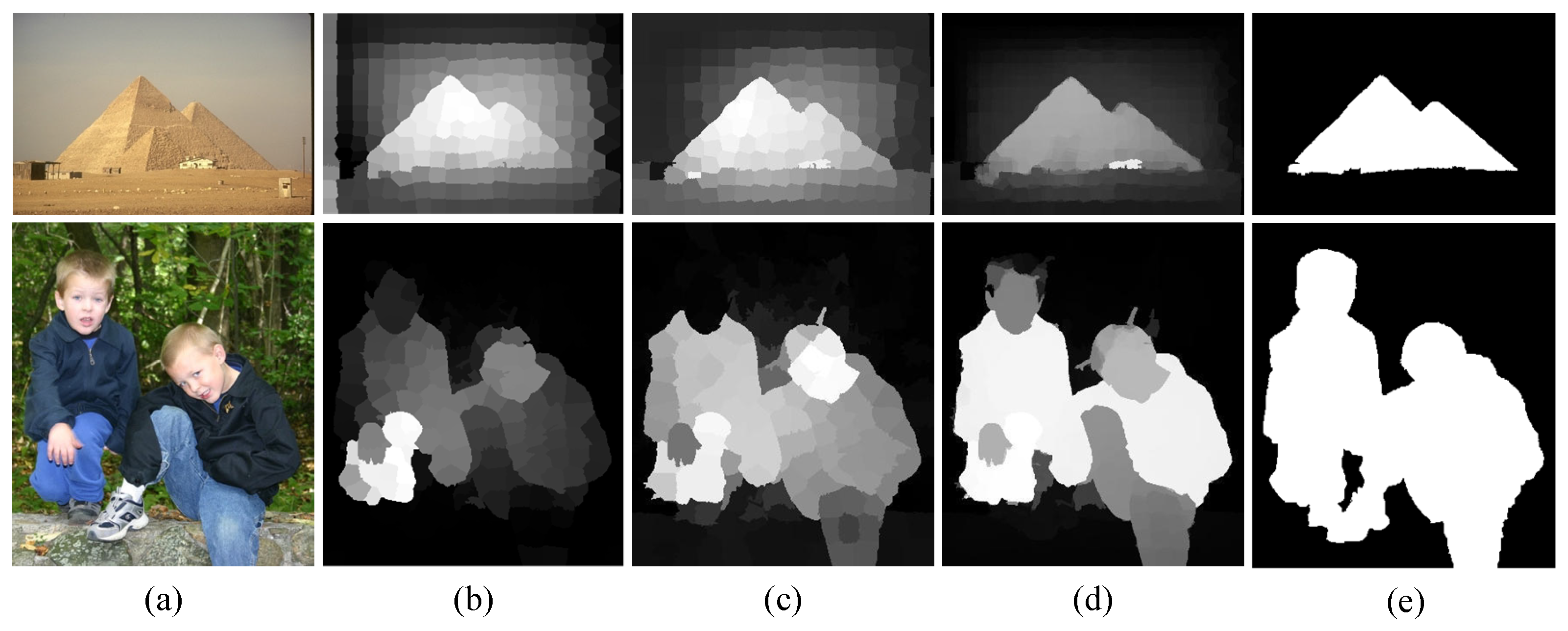
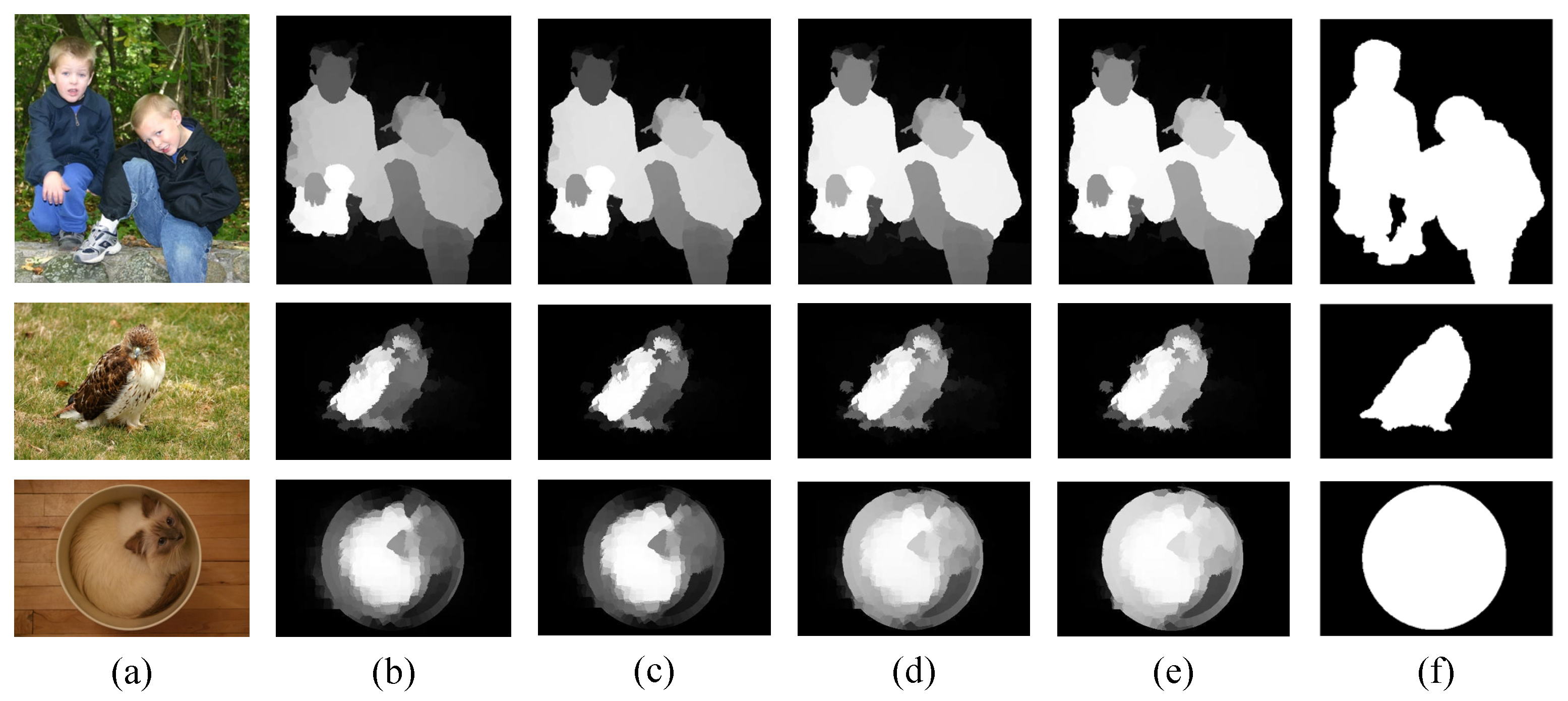
It is worth mentioning that the bottom-up models [13,14] are pioneer, graph-based methods that have shown promising performance with simplicity and efficiency. These methods mainly contain two aspects, i.e., graph construction and foreground/background seed selection. For saliency detection, graph construction is a critical issue. Traditionally, graph models depend on the Gaussian kernel function to compute affinity matrices in a single-view feature (CIElab color). Background seeds follow the boundary prior (the boundary patches are mostly background). The single-view feature cannot contain rich information about an image. To address this problem, graph models [18,19,20,21] were further constructed on multi-view low-level features for salient object detection. However, the above methods have two limitations. On the one hand, these traditional graphs are constructed from the Gaussian kernel function and may often be corrupted by noise. On the other hand, they fail to efficiently exploit both the consistency and complementary intrinsic structure of multi-view features. Both degrade saliency performance (Figure 1).
To overcome the aforementioned limitations, on the basis of the existing graph models, we propose a novel, multi-scale pure graph with multi-view subspace clustering for salient object detection. It builds upon two-stage multi-scale graphs and follows the background to compute the saliency score of each superpixel. In detail, to capture the local structures of multi-view low-level features, we first utilized the Gaussian kernel function to calculate the traditional graph matrix. Secondly, to further depict the global structure and eliminate the noise of multi-view low-level features, multi-view low-rank sparse subspace clustering [22] was applied to generate a shared affinity matrix. Afterward, the traditional graph matrix and affinity matrix were decomposed by singular value decomposition (SVD). In order to exploit the consistency and complementary intrinsic structure of multi-view low-level features, a joint affinity graph matrix was learned from multi-view subspace clustering based on a low-rank representation with diversity regularization and a rank constraint [23]. Based on these graph matrices, we constructed two-stage multi-scale graphs for graph-based manifold ranking. The main contributions are summarized as follows:
1.
To depict the global structure and remove the noise of multi-view low-level features, multi-view low-rank sparse subspace clustering was applied to induce a shared affinity graph matrix.
2.
To further capture the consistency and complementary intrinsic structure of multi-view features, multi-view subspace clustering was explored based on a low-rank representation with diversity regularization.
3.
To clearly describe the local and global structure of multi-view low-level features, two-stage multi-scale pure graphs were constructed based on the above graph matrices.
4.
Extensive experiments demonstrate that our two-stage, multi-scale pure graphs consistently achieve better saliency performance than several state-of-the-art graph models on five benchmark datasets.
The rest of this paper is organized as follows. Section 2 describes the works related to the proposed method. Section 3 introduces the main aspects of our designed framework. Section 4 presents the experiments and comparisons. Section 5 gives a discussion of the proposed method. Finally, Section 6 concludes our work.

2. Related Work

In the early stage of graph-based saliency detection, in view of these representative graph-based saliency detection methods [14,24,25,26], researchers mainly adopted the CIElab color feature to compute the affinity matrix. However, these graph models only use the CIElab color space and are unable to present the rich diversity of salient objects and backgrounds. Even worse, traditional graphs fail to capture the global structure of an image.
In particular, the work that inspired our proposed method is that featuring graph-based manifold ranking (GMR) [14], which has attracted a lot of attention in salient object detection. In this method, an RGB image is mapped onto a graph G = ( V , E ) with N nodes { v 1 , v 2 , . . . , v N } and a set of edges E. Traditionally, E is denoted by an affinity graph matrix W = [ w i j ] N × N and w i j is calculated by
w i j = e x i x j σ 2 i f   j N i 0 o t h e r w i s e
where x i and x j represent the mean scores of superpixels v i and v j in the feature space, respectively. σ is a constant. N i denotes the neighbors of superpixel v i . From the graph matrix W = [ w i j ] N × N , the corresponding degree matrix D = d i a g { d 11 , . . . , d N N } is obtained, where d i i = i N w i j . Accordingly, let y = [ y 1 , y 2 , . . , y N ] T be a indication vector, in which y i = 1 if x i is a query and y i = 0 otherwise. The optimal ranking solution of queries is derived by solving the optimization formula:
f * = arg min f 1 2 ( i , j = 1 N w i j f i d i i f j d j j 2 + μ i = 1 N f i y i 2 )
where the first term ( i , j = 1 N w i j f i d i i f j d j j 2 ) represents the smoothness constraint. The second term ( i = 1 N f i y i 2 ) represents the fitting constraint. The parameter μ controls the balance between these two terms. f * is the ranking results. When setting the derivative of Equation (2) to be 0, the ranking results f * is equal to
f * = ( D α S ) 1 y
where S denotes a normalized Laplacian matrix, S = D 1 / 2 W D 1 / 2 , and α = 1 1 + μ = 0.99 .
To suit salient object detection, an unnormalized Laplacian matrix is embeded into Equation (3) and then the final ranking result is generated as
f * = ( D α W ) 1 y
The key contribution of graph-based manifold ranking is two-stage “superior” graphs. For a “superior” graph matrix W R N × N , each element w i j is an edge weight that reflects the similarity between two adjacent nodes/superpixels x i and x j of an input image. Inspired by this, researchers [18,20,27] extracted the multi-view appearance feature from an image and developed the corresponding graph-based approaches. They individually computed the traditional graph matrix in each appearance feature and achieved the final graph matrix through linear fusion or vector dot product. However, these approaches still cannot capture the global structure. Furthermore, their graphs are insufficient to possess consistency and complementary intrinsic structures from the multi-view features and do not obtain significantly enhanced saliency results. Benefiting from the high-level features of deep learning [28,29] that contain rich semantic concepts of salient objects, several improved graph-based algorithms [30,31,32,33] have been proposed. These methods construct traditional graph matrices by extracting the multi-view features containing high-level semantic information and appearance features. Since the high-level semantic information can effectively describe the salient objects, these algorithms achieve better saliency performance. However, the high-level semantic information needs plenty of time to train the sample datasets. Moreover, the pooling of convolutional neural networks seriously blurs the position information of salient objects. In recent years, with the superior performance of deep learning [34,35], convolutional neural networks [36,37] and attention-based graph models [38,39,40] have been developed to perform salient object detection and have achieved outstanding saliency results. But, they still have a common shortcoming whereby they require a huge amount of labeled data along with a GPU-enabled system. In this study, different from all the aforementioned salient object detection methods, our proposed method explicitly explores subspace clustering and constructs a robust graph model of the multi-view low-level features in saliency objects. Fortunately, compared with unsupervised graph-based saliency models with multi-view low-level features, our proposed method generates promising performance and breaks through the limitation of traditional graph models.

3. Methodology

A diagram of our proposed method is shown in Figure 2, and the details will be elaborated upon below.

3.1. Multi-View Feature Extraction

To effectively describe the difference between salient objects and background, our proposed method firstly extracts 64-dimension low-level features, as given in Table 1. Secondly, SLIC [41] is carried out to over-segment the input image into N nonoverlapping superpixels P = { P 1 , P 2 , , P N } . For each superpixel P i , each view feature matrix is represented as X ( v ) = { x 1 ( v ) , x 2 ( v ) , , x N ( v ) } R d v × N , where v = { 1 , 2 , . . , V } .

3.2. Multi-View Pure Graph Construction

This section includes the traditional graph matrix computation and joint affinity matrix learning with multi-view subspace clustering.

3.2.1. Adjacent Graph

Based on the suitability of the traditional graph matrix in salient object detection, the similarity between any two adjacent nodes P i and P j in multi-view features is calculated as follows:
w i j ( l ) = e x i ( l ) x j ( l ) 2 σ 2 i f j N i 0 o t h e r w i s e
w i j ( o ) = e x i ( o ) x j ( o ) 2 σ 2 i f j N i 0 o t h e r w i s e
where x i ( l ) and x j ( l ) represent the mean values of superpixels P i and P j in CIElab color features, respectively. x i ( o ) and x j ( o ) represent the mean values of superpixels P i and P j in other multi-view features, respectively. σ is a constant parameter that controls the degree of similarity. To integrate these two graph matrices W ( o ) = [ w i j ( o ) ] N × N and W ( l ) = [ w i j ( l ) ] N × N , the traditional graph matrix is generated by
W ( T ) = ( W ( l ) ) 2 + ( W ( o ) ) 2

3.2.2. Affinity Graph Learning

The multi-view features X ( v ) = { V ( 1 ) ; V ( 2 ) ; ; X ( V ) } R d × n should share consensus information because different features represent an input image simultaneously. Firstly, to eliminate the confusion of noise, an affinity matrix shared among multi-views is learned with low-rank and sparsity constraints, then defined as
min C ( 1 ) , C ( 2 ) , . . . , C ( V ) = v = 1 V ( β 1 C ( v ) * + β 2 C ( v ) 1 + λ ( v ) C ( v ) C * F 2 ) s . t . X v = X v C v , d i a g ( C v ) = 0 .
where C ( v ) represents the low-rank representation matrix of the v-th feature, C * represents the consensus low-rank representation matrix of all views, and the parameters β 1 , β 2 , and λ ( v ) control the trade-off between low-rank and sparsity terms, respectively. In this study, we set β 1 = 0.1 , β 2 = 1 β 1 , λ ( v ) = 0.3 , V = 8 . The optimization problem of this objective function is solved with the method [22]. Then, the affinity matrix is obtained by
W ( C ) = | C * | + | C * | T 2
To better explore the local similarity information of the traditional graph matrix W ( T ) and global similarity information of the affinity matrix W ( C ) , we utilize the Hadamard product to combine these two matrices, as follows:
W ( T C ) = W ( C ) ˜ T W ( T ) W ( C ) ˜ + W ( T ) ˜ T W ( C ) W ( T ) ˜
where ∘ represents the Hadamard product of N × N matrices. The Hadamard product can reduce the computational complexity of the matrix fusion and is insensitive to the saliency results of our proposed method. Regarding the matrices W ( C ) and W ( T ) , the angular information of the principal directions of any two low-rank vectors probably extracted from the same subspace has a higher value than that of those extracted from different subspaces. Specifically, we calculate W ( C ) ˜ = U ( C ) Σ ( V ( C ) ) T and W ( T ) ˜ = U ( T ) Σ ( V ( T ) ) T , which represent the SVDs of W ( C ) and W ( T ) , respectively. Thus, W ( T C ) with global clustering can be used to refine the neighbors of the traditional graph. Further, in order to sufficiently exploit consistency and complementary information among multi-view features, the graph regularization term and rank constraint are simultaneously mixed to formulate the objective model and then a joint affinity matrix is learned and obtained as follows:
min Z ^ , E ( v ) , w Z ^ * + v = 1 V w ( v ) E ( v ) 2 , 1 + λ w T H w + β T r ( Z ^ L s Z ^ T ) s . t . X ( v ) = X ( v ) Z ^ + E ( v ) , w T 1 V = 1 , r a n k ( L s ) = N C ,
where Z ^ is the joint representation matrix of the multi-view features. E ( v ) is the representation residual matrix of the v-th view. L s ( T C ) is the Laplacian matrix of the graph matrix W ( T C ) . λ and β are two positive balance parameters, which are set to λ = 1 and β = 1 . C represents different classes of the multiview data, setting C = 10 . H = [ H i , j ] V × V R V × V and H i , j = T r ( T i T T j ) represent the similarity between the i-th and j-th views, where T i = D i 1 S i ( i = 1 , 2 , , V ) is the probability transition matrix of the random walk of the i-th view. 1 V R V is a vector and its elements are set as 1. Given a vector w R + V , a diversity regularization term is obtained as follows:
min w R + V i , j = 1 V w i w j H i , j = w T Hw s . t . w T 1 = 1
We adopt the augmented Lagrange multiplier with alternating direction minimizing (ALM-ADM) to optimize the objective function Equation (11). This objective function is solved via [23]. Accordingly, the joint affinity matrix is achieved by
W ( Z ) = | Z ^ | + | Z ^ | T 2
In order to compute saliency maps with homogeneity and integrity, W ( Z ) is further normalized as follows:
W ( Z ) = ( D ( Z ) ) 1 · W ( Z )
where D ( Z ) is the degree matrix of the graph matrix W ( Z ) . On this basis, W ( Z ) is applied to strengthen the above graph matrix. Accordingly, the graph matrix of first-stage graph-based manifold ranking is
W ( 1 ) = ( W ( Z ) * ) T W ( T C ) W ( Z ) + η 1 ( W ( Z ) ) T W ( T ) W ( Z )
Inspired by the background prior, the coarse saliency score is computed by propagating the background seeds y on the graph, which is formulated as
f * ( 1 ) = ( D ( 1 ) α W ( 1 ) ) 1 y
where y { y t , y d , y l , y r } , in which y t , y d , y l , and y r represent the top, down, left, and right boundaries of an image, respectively. f * ( 1 ) is the saliency result of the first-stage graph-based manifold ranking.
After segmenting f * ( 1 ) by the threshold value κ · m e a n ( f * ( 1 ) ) , the foreground seed y f is produced. Thereby, for the faithful propagation of foreground seed y f , another “good” graph matrix is expected to be constructed. Considering the saliency f * ( 1 ) , a new graph matrix is computed as
W ( 2 ) = ( W ( T ) ) T W ( f ) W ( T ) + η 2 ( W ( Z ) * ) T W ( f ) W ( Z ) *
where W ( f ) is the traditional graph matrix by using the saliency f * ( 1 ) . Finally, the saliency map is achieved by Algorithm 1:
f * ( 2 ) = ( D ( 2 ) α W ( 2 ) ) 1 y f
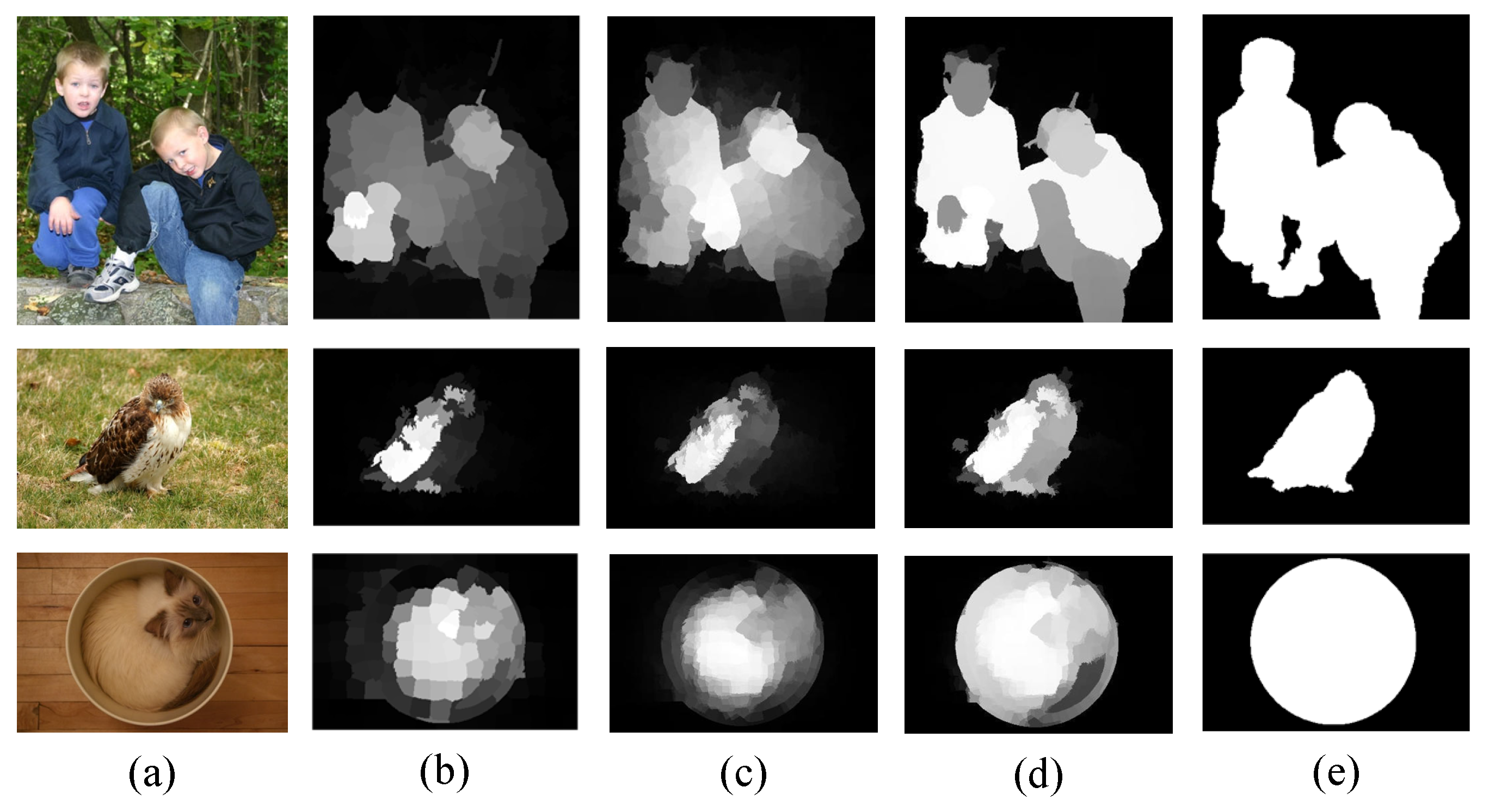
The saliency maps of the proposed framework are presented in Figure 3.
Computational Complexity: In Algorithm 1, two main computational complexities solve the objective functions (Equations (8) and (11)). Following [22], the computational complexity of solving the objective functions in Equation (8) is O ( T V N 3 ) , where T is the number of iterations, V is the number of views, and N is the number of superpixels. In addition, the computational complexity of solving the objective functions in Equation (11) is O ( d i 2 N + d i N 2 + N 3 ) by following reference [23], where d i is the dimension of each view.
Algorithm 1 Multi-scale pure graphs with multi-view subspace clustering for salient object detection
Require: Multi-view features X , background seeds y { y t , y d , y l , y r } .
Ensure: Saliency result f * ( 2 ) .
  1:
Initially compute traditional graph matrices W ( l ) = [ w i j ( l ) ] N × N and W ( o ) = [ w i j ( o ) ] N × N by Equation (5) and Equation (6) respectively.
  2:
Fuse traditional graph matrices W ( l ) = [ w i j ( l ) ] N × N and W ( o ) = [ w i j ( o ) ] N × N to generate W ( T ) by Equation (7).
  3:
Learn affinity graph matrix W ( C ) by the objective function Equations (8) and (9).
  4:
Combine W ( C ) and W ( T ) and produce W ( T C ) by Equation (10).
  5:
Achieve affinity graph matrix W ( Z ) by the objective function Equations (11) and (13).
  6:
Normalize affinity graph matrix W ( Z ) and obtain W ( Z ) * by Equation (14).
  7:
Construct first-stage graph matrix W ( 1 ) by Equation (15).
  8:
Propagate background seeds y { y t , y d , y l , y r } and compute coarse saliency map f * ( 1 ) by Equation (16).
  9:
Construct second-stage graph matrix W ( 2 ) by Equation (17).
10:
Obtain foreground seeds by segmenting f * ( 1 ) .
11:
Propagate foreground seeds y f and calculate fine saliency result f * ( 2 ) by Equation (18).

4. Experimental Design and Analysis

In this section, we evaluate the saliency performance of the proposed method on five public RGB datasets, which provide qualitative and quantitative comparisons with ten state-of-the-art methods, and carry out some effectiveness analysis of ablation experiments.

4.1. Experimental Setup

4.1.1. Implementation Details

All extensive experiments were performed in MATLAB 2016b on an Intel(R) Core(TM) i5-3700K with CPU @ 3.40 GHz and 32.0 GB of RAM. In the proposed framework, the numbers of multi-scale superpixels were set as 200, 300, and 400.

4.1.2. Benchmark Dataset

To demonstrate the effectiveness of the proposed approach, we conducted extensive experiments on five public RGB saliency detection datasets, named ECSSD [46], SOD [47], DUTOMRON [46], HUK-IS [48], and SED2 [49].
ECSSD has 1000 images of complex scenes with meaningful and rich semantic concepts.
SOD contains 300 challenging images from the Berkeley segmentation dataset, in which most images have several objects, which is challenging for bottom-up models.
DUTOMRON contains 5168 images with structural complexity and at least one object in a scene.
HUK-IS contains 4447 images with multiple salient objects.
SED2 contains 100 images and each image has two salient objects.

4.1.3. Baseline Models

To show the superior saliency performance of the proposed method, we compared the proposed method with ten state-of-the-art methods, including DRFI [13], GMR [14], RBD [50], BSCA [26], SMD [42], DP2-LSG [51], RCRR [52], WMR [18], PDP [53], AME [54], and HCA [55].
GMR is the baseline of our method.
AME is a promising graph-based salient object detection approach among existing bottom-up models in which the graph is constructed by multi-view high-level features.
HCA is an improvement of BSCA, where BSCA is named single cellular automata. It utilizes multi-view high-level features and multi-view low-level features.
SMD is a saliency detection method based on low-rank matrix recovery theory that exploits multi-view low-level features.
DRFI is a deep learning approach that exploits multi-view low-level features to highlight salient regions and achieves remarkable saliency performance.
Others are representative graph-based methods.

4.1.4. Evaluation Metrics

To achieve a faithful evaluation of all experimental results, the comparison experiments relied on eight evaluation metrics, such as the precision–recall (PR) curve [14], S-measure [56], E-measure [57], F-measure ( F m ), mean absolute error (MAE) [12], area under curve (AUC), overlap ratio (OR) [42], and weighted F-measure [58].
PR: in the precision–recall (PR) curve, the precision was the correct proportion of the detection results and the recall was the proportion of correct detection results in the ground truth (GT). They were defined as follows:
P r e c i s i o n = | M G T | | M | , R e c a l l = | M G T | | G T |
where M denotes the binarized map of a saliency map and GT represents the corresponding ground truth (GT).
S-measure was adopted to assess the detection performance and counted region-aware and object-aware structural similarity among the saliency map and the corresponding ground-truth map, which was computed by
S β = β · S o + ( 1 β ) · S r
where S o and S r are the region-aware and object-aware structural similarity measures, respectively.
E-measure was an enhanced-alignment measure that integrated the local pixel score with the image-level mean score and computed the statistics for image levels and matching information of local pixels. It was defined as
E ξ = 1 W × H i = 1 W j = 1 H θ ( ξ )
where θ ( ξ ) denotes the enhanced-alignment matrix.
F-measure was used to obtain an overall measure for the saliency results and was formulated as
F β = ( 1 + β 2 ) · P r e c i s i o n · R e c a l l β 2 · P r e c i s i o n + R e c a l l
β 2 was set to 0.3 to strengthen the precision. Based on this, the weighted F-measure was computed by
F β ω = ( 1 + β 2 ) · P r e c i s i o n ω · R e c a l l ω β 2 · P r e c i s i o n ω + R e c a l l ω
MAE was an assistant measure that calculated the average difference between the saliency map and the corresponding ground truth:
M A E = 1 W × H i = 0 W 1 j = 0 H 1 | S ( i , j ) G T ( i , j ) |
A lower computed value meant a better performance.
AUC was defined as the area under the ROC curve; the ROC curve was obtained by computing the true positive rate (TPR) and false positive rate (FPR) under different thresholds.

4.2. Comparison with State-of-the-Art Methods

This section comprehensively evaluates and analyzes both quantitative and qualitative comparisons of the experimental results for the ECSSD, SOD, DUTOMRON, HUK-IS, and SED2 datasets.
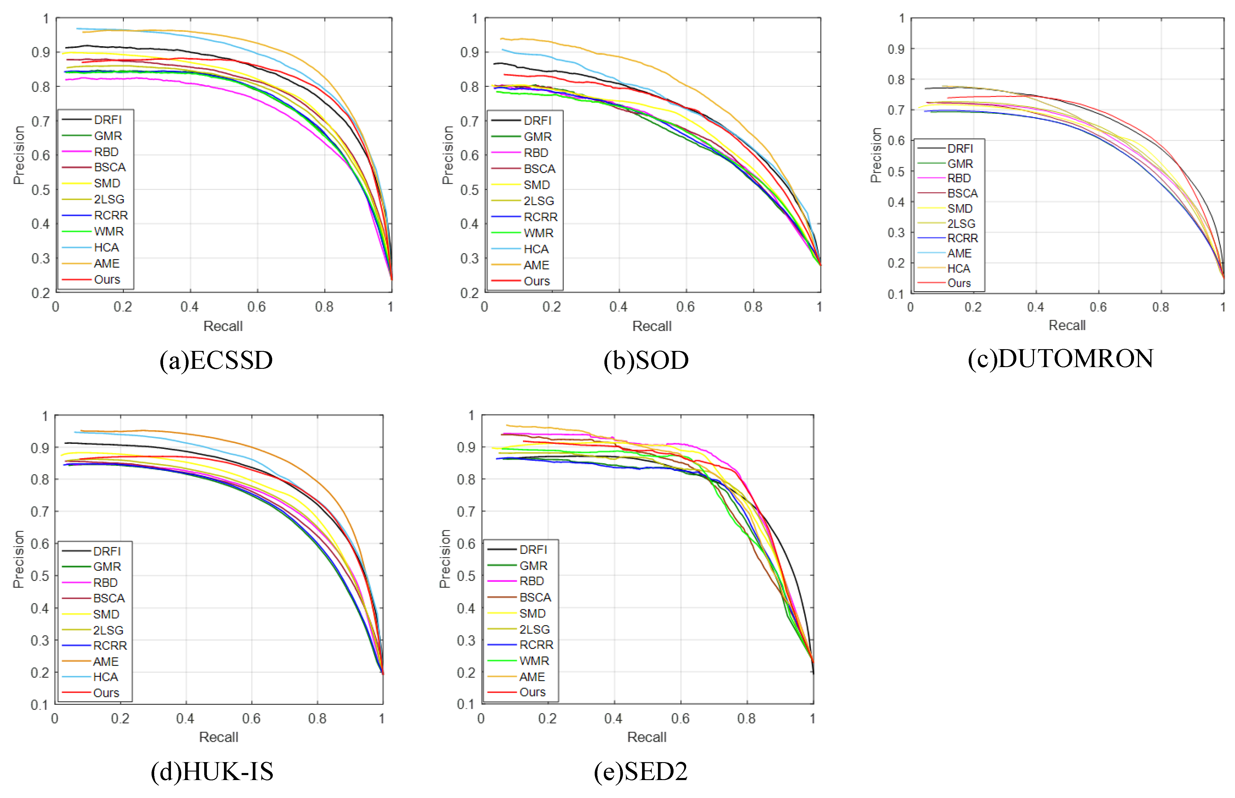
Figure 4 shows the PR curves of our proposed method and other compared methods. It is noteworthy that our method significantly outperformed other state-of-the-art methods for DUTOMRON, ECSSD, SOD, and HUK-IS, and our method was clearly better than the other baseline methods except for AME and HCA. The most important factor was that AME and HCA utilize deeper or learned semantic features, while our proposed method only employs multi-view low-level features. On SED2, our method also achieved a better result. Moreover, Table 2, Table 3, Table 4, Table 5 and Table 6 present the quantitative comparison results, including the S-measure, E-measure, F-measure, MAE, AUC, WF, and OR matrices. Table 2, Table 3, Table 4 and Table 5 further demonstrate the superiority of our proposed method on ECSSD, SOD, HUK-IS, and DUTOMRON. As shown in Table 6, our method achieved considerable performance compared with the baseline methods.
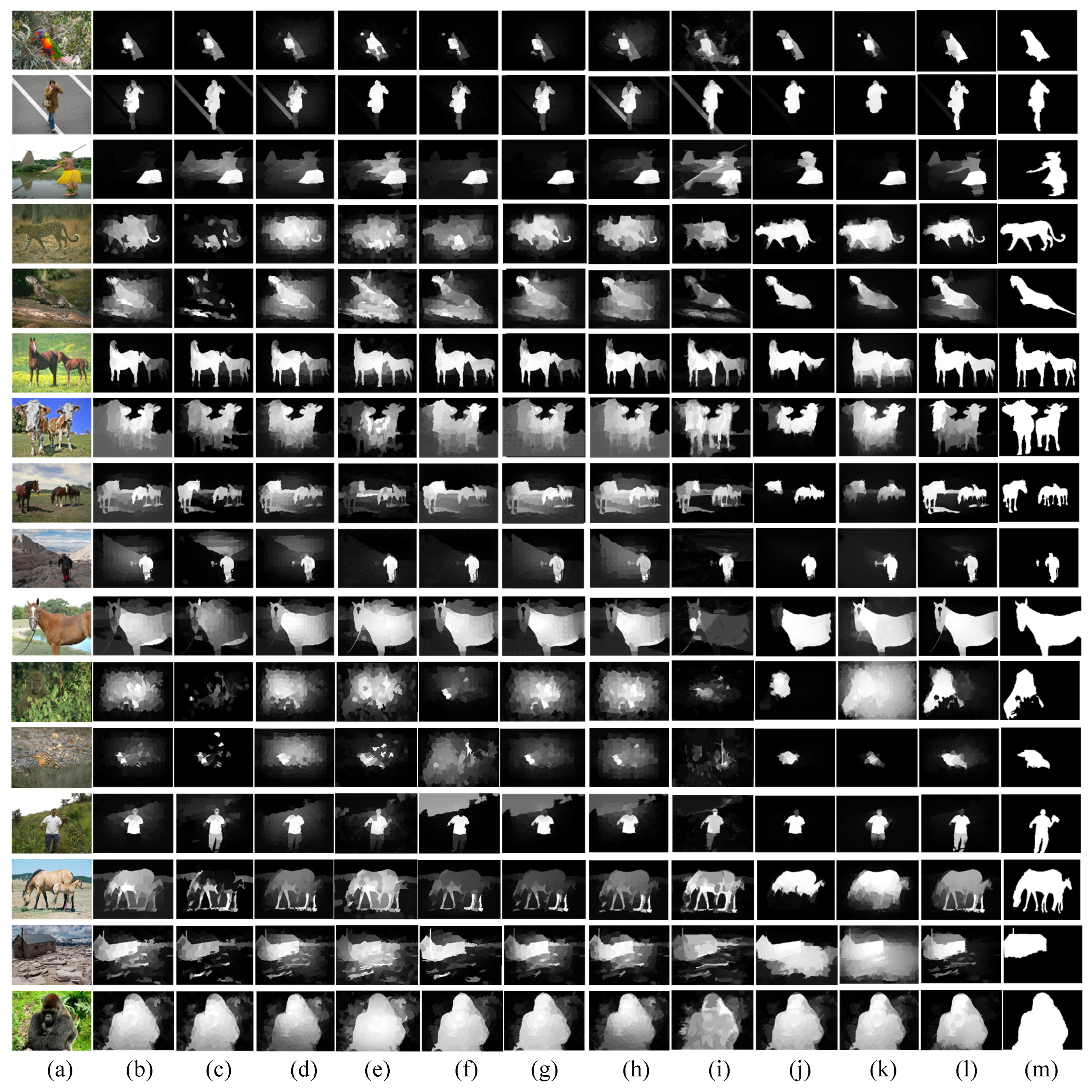
Visual comparisons of saliency maps of different algorithms in typical scenarios are shown in Figure 5. Intuitively, our method could accurately extract the salient objects in complex scenes. Even if salient objects were extremely similar to the surroundings (Image 4, 5, 11, 12, 15), the proposed method could still generate better saliency performance. These examples obviously illustrate the effectiveness and robustness of the proposed method. In total, visual comparisons clearly demonstrate that our proposed method performed better than the state-of-the-art methods on challenging scenes.

4.3. Comparison of Ablation Experiments

In this subsection, we describe the related ablation experiments, including the graph model analysis and each stage of graph contribution.
In the first stage of graph-based manifold ranking, the key matter is the newly constructed graph W ( 1 ) . Based on this, we tested the proposed scheme with traditional multi-view graph W T and new multi-view graph W ( 1 ) . From Figure 6a and Table 7, we can observe that the new multi-view graph W ( 1 ) performed significantly better than the traditional multi-view graph W T and baseline method. Meanwhile, Figure 7 displays the superiority of the proposed method using visual comparisons. As for the contributions of the two-stage graphs, Figure 6b and Table 8 present the PR curves and other quantitative results. It can be seen that the affinity graph W ( T C ) contributed to the two-stage graph-based manifold ranking. Table 8 quantitatively demonstrates the contribution of the proposed second-stage graph. Figure 8 displays visual comparisons, further showing the progress from coarse to fine.
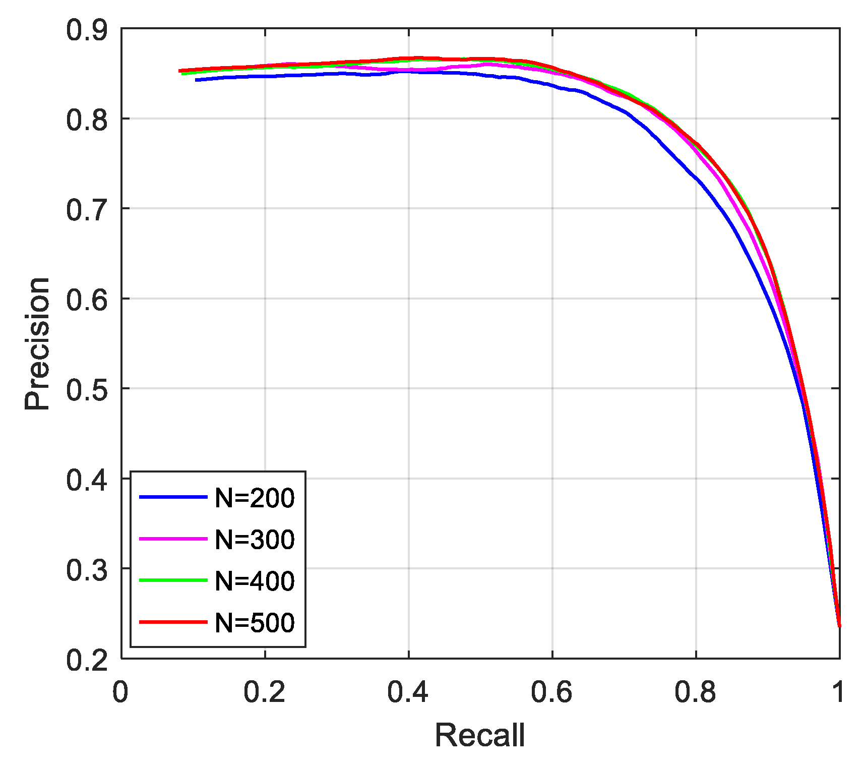
Finally, we analyzed the influence of superpixels with different numbers of superpixels, as shown in Figure 9 and Table 9. The best performance of the proposed method was obtained when the number of superpixels was set to N = 400 .

4.4. Extended Experiment on High-Resolution Dataset

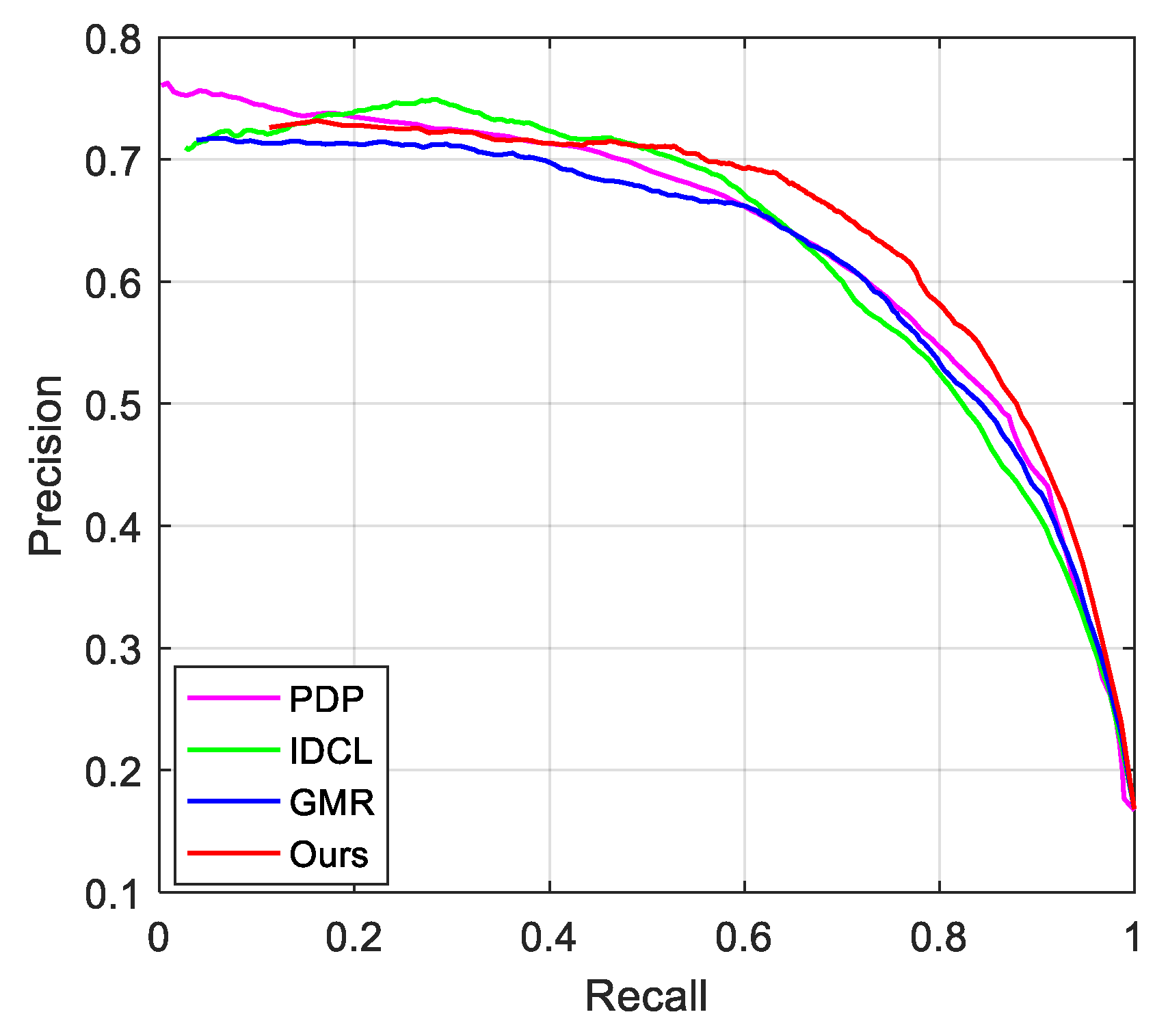
To demonstrate the potential applicability of our proposed method in broader contexts, we provide quantitative comparisons on a high-resolution dataset. Most graph-based saliency detection methods mainly focus on natural images with low resolutions, such as 400 × 400 or smaller, which limits their potential applications. Therefore, we tested our method on the high-resolution dataset (HRSOD) and compared it with graph-based models (GMR, IDCL) and the PDP method. Figure 10 shows the PR curves of the experimental methods on the HRSOD dataset, showing that the proposed method achieved the best performance improvement. The proposed method demonstrates a powerful ability to be used in practical applications compared to the three traditional graph-based saliency detection models.

4.5. Running Time

The computational time of the proposed method was analyzed on the ECSSD benchmark dataset. The proposed method was implemented on MATLAB 2016b on the 13th Gen Intel(R) Core(TM) i7-13700K with CPU @ 3.40 GHz and 32.0 GB of RAM. It took approximately 5.79 s on average to generate the saliency map for experimental images of 400 × 267 pixels. Table 10 shows the average time of our method and the baseline models. We found that our method was slower than the competitive methods but still outperformed them both considering the comprehensive evaluation performances. This was because the competitive models AME and HCA required a significant amount of time to train multi-view semantic features using neural networks.

5. Discussion

In this work, we explored graphs with low-level multi-view features and computed saliency scores by following the background prior. This could produce poor saliency results, as shown in Figure 11. For the challenging scenes, only low-level multi-view features caused an inability to identify salient objects. In a future study, we plan to exploit multi-view deep-level semantic information to construct a “good” graph matrix for hyperspectral images. In addition, it is worth mentioning that eye movement data can be formulated to describe clinically relevant regions in a medical image and potentially integrated into an artificial intelligence (AI) system for automatic diagnosis in medical imaging. Therefore, we will be committed to researching graph neural networks for saliency detection and applying them to chest X-rays.

6. Conclusions

In this paper, we proposed novel, multi-scale pure graphs with multi-view subspace clustering for salient object detection. This work presented two-stage graphs constrained by multi-view subspace clustering with sparsity and low rank and embedded them into manifold ranking to compute a saliency map. This could upgrade saliency performance using the propagation on the graph model that exploited consistency and complementary information among multi-view features. Both methods effectively boosted the capability of the graph model. To validate the promising performance of the proposed method in terms of standard evaluation indexes, experiments on several RGB benchmark datasets and comparisons with several state-of-the-art baseline methods were carried out. The superior saliency performance enhancement demonstrates the good generalization capability of our proposed saliency detection framework.

Author Contributions

Conceptualization, M.W. and F.W.; Methodology, M.W. and F.W.; Software, H.Y. and W.W.; Validation, M.W., F.W. and H.Y.; Formal analysis, M.W. and F.W.; Resources, F.W.; Data curation, M.W.; Writing—original draft, M.W.; Writing—review and editing, M.W., Y.Z. and F.W.; Visualization, H.Y.; Supervision, M.W., Y.Z. and F.W.; Project administration, M.W.; Funding acquisition, M.W., Y.Z. and F.W. All authors have read and agreed to the published version of the manuscript.

Funding

This work was financially supported in part by the National Natural Science Foundation of China under grant 12401673, the Graduate Education Comprehensive Reform Project of Xi’an Shiyou University under grant 2023-X-YJG-021, the Deep Earth Probe and Mineral Resources Exploration-National Science and Technology Major Project under grant 2024ZD1004406, the Natural Science Basic Research Program of Shaanxi under grant 2024JC-YBQN-0670, and the Youth Innovation Team of Shaanxi Universities (Yi Zhang).

Data Availability Statement

All data generated or analysed during this study are included in this article.

Acknowledgments

We sincerely thank all the creators and funding programs that were involved in the writing of this paper.

Conflicts of Interest

The authors declare no conflicts of interest.

References

  1. Hsu, K.J.; Lin, Y.Y.; Chuang, Y.Y. DeepCO3: Deep Instance Co-Segmentation by Co-Peak Search and Co-Saliency Detection. In Proceedings of the 2019 IEEE/CVF Conference on Computer Vision and Pattern Recognition (CVPR), Long Beach, CA, USA, 15–20 June 2019; pp. 8838–8847. [Google Scholar] [CrossRef]
  2. Yang, X.; Qian, X.; Xue, Y. Scalable Mobile Image Retrieval by Exploring Contextual Saliency. IEEE Trans. Image Process. 2015, 24, 1709–1721. [Google Scholar] [CrossRef] [PubMed]
  3. Ma, J.; Tang, L.; Xu, M.; Zhang, H.; Xiao, G. STDFusionNet: An Infrared and Visible Image Fusion Network Based on Salient Target Detection. IEEE Trans. Instrum. Meas. 2021, 70, 5009513. [Google Scholar] [CrossRef]
  4. Wang, Q.; Chen, F.; Xu, W. Saliency selection for robust visual tracking. In Proceedings of the 2010 IEEE International Conference on Image Processing, Hong Kong, China, 26–29 September 2010; pp. 2785–2788. [Google Scholar]
  5. Deng, T.; Yang, K.; Li, Y.; Yan, H. Where Does the Driver Look? Top-Down-Based Saliency Detection in a Traffic Driving Environment. IEEE Trans. Intell. Transp. Syst. 2016, 17, 2051–2062. [Google Scholar] [CrossRef]
  6. Itti, L.; Koch, C.; Niebur, E. A Model of Saliency-based Visual Attention for Rapid Scene Analysis. IEEE Trans. Pattern Anal. Mach. Intell. 1998, 20, 1254–1259. [Google Scholar] [CrossRef]
  7. Schölkopf, B.; Platt, J.; Hofmann, T. Graph-Based Visual Saliency. In Advances in Neural Information Processing Systems 19: Proceedings of the 2006 Conference; MIT Press: Cambridge, MA, USA, 2007; pp. 545–552. [Google Scholar]
  8. Hou, X.; Zhang, L. Saliency Detection: A Spectral Residual Approach. In Proceedings of the 2007 IEEE Conference on Computer Vision and Pattern Recognition, Minneapolis, MN, USA, 17–22 June 2007; pp. 1–8. [Google Scholar]
  9. Achanta, R.; Estrada, F.; Wils, P.; Süsstrunk, S. Salient Region Detection and Segmentation; Springer: Berlin, Germany, 2008. [Google Scholar] [CrossRef]
  10. Achantay, R.; Hemamiz, S.; Estraday, F.; Süsstrunky, S. Frequency-tuned salient region detection. In Proceedings of the 2009 IEEE Computer Society Conference on Computer Vision and Pattern Recognition Workshops, CVPR Workshops 2009, Miami, FL, USA, 20–25 June 2009; pp. 1597–1604. [Google Scholar] [CrossRef]
  11. Cheng, M.M.; Zhang, G.X.; Mitra, N.; Huang, X.; Hu, S.M. Global Contrast Based Salient Region Detection. IEEE Trans. Pattern Anal. Mach. Intell. 2011, 37, 409–416. [Google Scholar] [CrossRef]
  12. Perazzi, F.; Krähenbühl, P.; Pritch, Y.; Hornung, A. Saliency filters: Contrast based filtering for salient region detection. In Proceedings of the 2012 IEEE Conference on Computer Vision and Pattern Recognition, Providence, RI, USA, 16–21 June 2012; pp. 733–740. [Google Scholar]
  13. Jiang, H.; Wang, J.; Yuan, Z.; Wu, Y.; Zheng, N.; Li, S. Salient Object Detection: A Discriminative Regional Feature Integration Approach. In Proceedings of the IEEE Conference on Computer Vision and Pattern Recognition (CVPR), Portland, OR, USA, 23–28 June 2013; pp. 2083–2090. [Google Scholar]
  14. Yang, C.; Zhang, L.; Lu, H.; Ruan, X.; Yang, M.H. Saliency Detection via Graph-Based Manifold Ranking. In Proceedings of the IEEE Conference on Computer Vision and Pattern Recognition (CVPR), Portland, OR, USA, 23–28 June 2013; pp. 3166–3173. [Google Scholar]
  15. Li, X.; Zhao, L.; Wei, L.; Yang, M.H.; Wu, F.; Zhuang, Y.; Ling, H.; Wang, J. DeepSaliency: Multi-Task Deep Neural Network Model for Salient Object Detection. IEEE Trans. Image Process. 2015, 25, 3919–3930. [Google Scholar] [CrossRef]
  16. Liu, N.; Han, J. DHSNet: Deep hierarchical saliency network for salient object detection. In Proceedings of the 2016 IEEE Conference on Computer Vision and Pattern Recognition (CVPR), Las Vegas, NV, USA, 27–30 June 2016; pp. 678–686. [Google Scholar]
  17. Li, G.; Yu, Y. Visual Saliency Detection Based on Multiscale Deep CNN Features. IEEE Trans. Image Process. 2016, 25, 5012–5024. [Google Scholar] [CrossRef]
  18. Zhu, X.; Tang, C.; Wang, P.; Xu, H.; Wang, M.; Tian, J. Saliency Detection via Affinity Graph Learning and Weighted Manifold Ranking. Neurocomputing 2018, 312, 239–250. [Google Scholar] [CrossRef]
  19. Zhang, M.; Pang, Y.; Wu, Y.; Du, Y.; Sun, H.; Zhang, K. Saliency Detection via Local Structure Propagation. J. Vis. Commun. Image Represent. 2018, 52, 131–142. [Google Scholar] [CrossRef]
  20. Ji, Y.; Zhang, H.; Tseng, K.K.; Chow, T.W.; Wu, Q.J. Graph Model-based Salient Object Detection Using Objectness and Multiple Saliency Cues. Neurocomputing 2018, 323, 188–202. [Google Scholar] [CrossRef]
  21. Liu, Y.; Han, J.; Zhang, Q.; Wang, L. Salient Object Detection via Two-Stage Graphs. IEEE Trans. Circuits Syst. Video Technol. 2019, 29, 1023–1037. [Google Scholar] [CrossRef]
  22. Brbić, M.; Kopriva, I. Multi-view low-rank sparse subspace clustering. Pattern Recognit. 2018, 73, 247–258. [Google Scholar] [CrossRef]
  23. Tang, C.; Zhu, X.; Liu, X.; Li, M.; Wang, P.; Zhang, C.; Wang, L. Learning a Joint Affinity Graph for Multiview Subspace Clustering. IEEE Trans. Multimed. 2019, 21, 1724–1736. [Google Scholar] [CrossRef]
  24. Jiang, B.; Zhang, L.; Lu, H.; Yang, C.; Yang, M.H. Saliency Detection via Absorbing Markov Chain. In Proceedings of the IEEE International Conference on Computer Vision (ICCV), Sydney, Australia, 1–8 December 2013; pp. 1665–1672. [Google Scholar]
  25. Zhou, L.; Yang, Z.; Yuan, Q.; Zhou, Z.; Hu, D. Salient Region Detection via Integrating Diffusion-Based Compactness and Local Contrast. IEEE Trans. Image Process. 2015, 24, 3308–3320. [Google Scholar] [CrossRef]
  26. Qin, Y.; Lu, H.; Xu, Y.; Wang, H. Saliency Detection via Cellular Automata. In Proceedings of the IEEE Conference on Computer Vision and Pattern Recognition (CVPR), Boston, MA, USA, 7–12 June 2015; pp. 110–119. [Google Scholar]
  27. Wang, F.; Wang, M.; Peng, G. Multiview diffusion-based affinity graph learning with good neighbourhoods for salient object detection. Appl. Intell. 2025, 55, 37. [Google Scholar] [CrossRef]
  28. Long, J.; Shelhamer, E.; Darrell, T. Fully Convolutional Networks for Semantic Segmentation. In Proceedings of the IEEE Conference on Computer Vision and Pattern Recognition (CVPR), Boston, MA, USA, 7–12 June 2015; pp. 3431–3440. [Google Scholar]
  29. Razavian, A.S.; Azizpour, H.; Sullivan, J.; Carlsson, S. CNN Features Off-the-Shelf: An Astounding Baseline for Recognition. In Proceedings of the 2014 IEEE Conference on Computer Vision and Pattern Recognition Workshops, Columbus, OH, USA, 23–28 June 2014; pp. 512–519. [Google Scholar] [CrossRef]
  30. Wang, Q.; Zheng, W.; Piramuthu, R. GraB: Visual Saliency via Novel Graph Model and Background Priors. In Proceedings of the IEEE Conference on Computer Vision and Pattern Recognition (CVPR), Las Vegas, NV, USA, 27–30 June 2016; pp. 535–543. [Google Scholar]
  31. Zhang, Y.Y.; Zhang, S.; Zhang, P.; Song, H.Z.; Zhang, X.G. Local Regression Ranking for Saliency Detection. IEEE Trans. Image Process. 2019, 29, 1536–1547. [Google Scholar] [CrossRef]
  32. Xia, C.; Zhang, H.; Gao, X.; Li, K. Exploiting background divergence and foreground compactness for Salient object detection. Neurocomputing 2019, 383, 194–211. [Google Scholar] [CrossRef]
  33. Deng, C.; Yang, X.; Nie, F.; Tao, D. Saliency Detection via a Multiple Self-Weighted Graph-Based Manifold Ranking. IEEE Trans. Multimed. 2020, 22, 885–896. [Google Scholar] [CrossRef]
  34. Zhang, K.; Li, T.; Shen, S.; Liu, B.; Chen, J.; Liu, Q. Adaptive Graph Convolutional Network with Attention Graph Clustering for Co-Saliency Detection. In Proceedings of the 2020 IEEE/CVF Conference on Computer Vision and Pattern Recognition (CVPR), Seattle, WA, USA, 13–19 June 2020; pp. 9047–9056. [Google Scholar] [CrossRef]
  35. Ji, W.; Li, X.; Wei, L.; Wu, F.; Zhuang, Y. Context-Aware Graph Label Propagation Network for Saliency Detection. IEEE Trans. Image Process. 2020, 29, 8177–8186. [Google Scholar] [CrossRef] [PubMed]
  36. Fang, X.; Jiang, M.; Zhu, J.; Shao, X.; Wang, H. GroupTransNet: Group transformer network for RGB-D salient object detection. Neurocomputing 2024, 594, 127865. [Google Scholar] [CrossRef]
  37. Zhong, M.; Sun, J.; Ren, P.; Wang, F.; Sun, F. MAGNet: Multi-scale Awareness and Global fusion Network for RGB-D salient object detection. Knowl.-Based Syst. 2024, 299, 112126. [Google Scholar] [CrossRef]
  38. Zhao, J.; Jia, Y.; Ma, L.; Yu, L. Recurrent Adaptive Graph Reasoning Network With Region and Boundary Interaction for Salient Object Detection in Optical Remote Sensing Images. IEEE Trans. Geosci. Remote Sens. 2024, 62, 5630720. [Google Scholar] [CrossRef]
  39. Wu, Z.; Lu, J.; Han, J.; Bai, L.; Zhang, Y.; Zhao, Z.; Song, S. Domain Separation Graph Neural Networks for Saliency Object Ranking. In Proceedings of the IEEE/CVF Conference on Computer Vision and Pattern Recognition (CVPR), Seattle, WA, USA, 16–22 June 2024; pp. 3964–3974. [Google Scholar]
  40. Yang, Q.; Gao, W.; Li, C.; Wang, H.; Dai, W.; Zou, J.; Xiong, H.; Frossard, P. 360Spred: Saliency Prediction for 360-Degree Videos Based on 3D Separable Graph Convolutional Networks. IEEE Trans. Circuits Syst. Video Technol. 2024, 34, 9979–9996. [Google Scholar] [CrossRef]
  41. Achanta, R.; Shaji, A.; Smith, K.; Lucchi, A.; Fua, P.; Süsstrunk, S. SLIC Superpixels Compared to State-of-the-Art Superpixel Methods. IEEE Trans. Pattern Anal. Mach. Intell. 2012, 34, 2274–2282. [Google Scholar] [CrossRef]
  42. Peng, H.; Li, B.; Ling, H.; Hu, W.; Xiong, W.; Maybank, S.J. Salient Object Detection via Structured Matrix Decomposition. IEEE Trans. Pattern Anal. Mach. Intell. 2017, 39, 818–832. [Google Scholar] [CrossRef] [PubMed]
  43. Lan, R.; Zhou, Y.; Tang, Y.Y. Quaternionic Weber Local Descriptor of Color Images. IEEE Trans. Circuits Syst. Video Technol. 2017, 27, 261–274. [Google Scholar] [CrossRef]
  44. Zhang, L.; Gu, Z.; Li, H. SDSP: A novel saliency detection method by combining simple priors. In Proceedings of the 2013 IEEE International Conference on Image Processing, Melbourne, Australia, 15–18 September 2013; pp. 171–175. [Google Scholar]
  45. Tong, N.; Lu, H.; Ruan, X.; Yang, M.H. Salient Object Detection via Bootstrap Learning. In Proceedings of the IEEE Conference on Computer Vision and Pattern Recognition (CVPR), Boston, MA, USA, 7–12 June 2015; pp. 1884–1892. [Google Scholar]
  46. Yan, Q.; Xu, L.; Shi, J.; Jia, J. Hierarchical Saliency Detection. In Proceedings of the IEEE Conference on Computer Vision and Pattern Recognition (CVPR), Portland, OR, USA, 23–28 June 2013; pp. 1155–1162. [Google Scholar]
  47. Movahedi, V.; Elder, J.H. Design and perceptual validation of performance measures for salient object segmentation. In Proceedings of the 2010 IEEE Computer Society Conference on Computer Vision and Pattern Recognition-Workshops, San Francisco, CA, USA, 13–18 June 2010; pp. 49–56. [Google Scholar]
  48. Li, G.; Yu, Y. Visual saliency based on multiscale deep features. In Proceedings of the IEEE Conference on Computer Vision and Pattern Recognition, Boston, MA, USA, 7–12 June 2015; pp. 5455–5463. [Google Scholar]
  49. Alpert, S.; Galun, M.; Brandt, A.; Basri, R. Image Segmentation by Probabilistic Bottom-Up Aggregation and Cue Integration. IEEE Trans. Pattern Anal. Mach. Intell. 2012, 34, 315–327. [Google Scholar] [CrossRef]
  50. Zhu, W.; Liang, S.; Wei, Y.; Sun, J. Saliency Optimization from Robust Background Detection. In Proceedings of the IEEE Conference on Computer Vision and Pattern Recognition (CVPR), Columbus, OH, USA, 23–28 June 2014; pp. 2814–2821. [Google Scholar]
  51. Zhou, L.; Yang, Z.; Zhou, Z.; Hu, D. Salient Region Detection Using Diffusion Process on a Two-Layer Sparse Graph. IEEE Trans. Image Process. 2017, 26, 5882–5894. [Google Scholar] [CrossRef]
  52. Zheng, Q.; Yu, S.; You, X. Coarse-to-fine salient object detection with low-rank matrix recovery. Neurocomputing 2020, 376, 232–243. [Google Scholar] [CrossRef]
  53. Xiao, X.; Zhou, Y.; Gong, Y.J. RGB-‘D’ Saliency Detection With Pseudo Depth. IEEE Trans. Image Process. 2019, 28, 2126–2139. [Google Scholar] [CrossRef]
  54. Zhang, L.; Ai, J.; Jiang, B.; Lu, H.; Li, X. Saliency Detection via Absorbing Markov Chain With Learnt Transition Probability. IEEE Trans. Image Process. 2018, 27, 987–998. [Google Scholar] [CrossRef] [PubMed]
  55. Qin, Y.; Feng, M.; Lu, H.; Cottrell, G.W. Hierarchical Cellular Automata for Visual Saliency. Int. J. Comput. Vis. 2018, 126, 751–770. [Google Scholar] [CrossRef]
  56. Fan, D.P.; Cheng, M.M.; Liu, Y.; Li, T.; Borji, A. Structure-Measure: A New Way to Evaluate Foreground Maps. In Proceedings of the IEEE International Conference on Computer Vision (ICCV), Venice, Italy, 22–29 October 2017; pp. 4548–4557. [Google Scholar]
  57. Fan, D.P.; Gong, C.; Cao, Y.; Ren, B.; Cheng, M.M.; Borji, A. Enhanced-alignment Measure for Binary Foreground Map Evaluation. In Proceedings of the Twenty-Seventh International Joint Conference on Artificial Intelligence Main Track, Stockholm, Sweden, 13–19 July 2018; pp. 698–704. [Google Scholar]
  58. Margolin, R.; Zelnik-Manor, L.; Tal, A. How to Evaluate Foreground Maps. In Proceedings of the 2014 IEEE Conference on Computer Vision and Pattern Recognition, Columbus, OH, USA, 23–28 June 2014; pp. 248–255. [Google Scholar] [CrossRef]
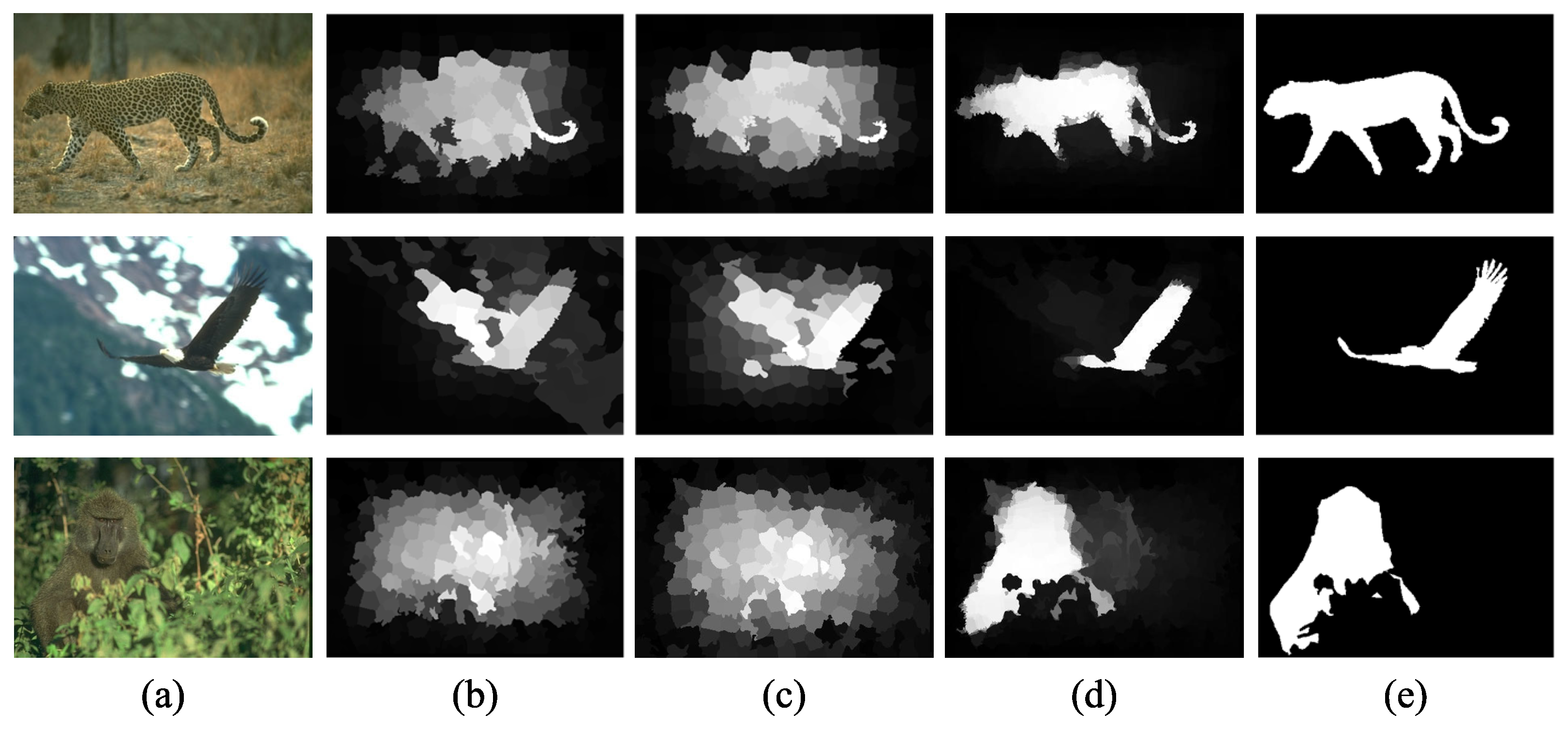
Figure 1. Visual results of graph-based manifold ranking. (a) Input image, (b) GMR [14], (c) WMR [18], (d) proposed method, (e) ground truth.
Symmetry 17 01262 g001
Figure 2. Diagram of our proposed method.
Symmetry 17 01262 g002
Figure 3. Visual results of the first-stage graph-based manifold ranking. (a) Input image, (b) GMR [14], (c) WMR [18], (d) proposed method, (e) ground truth.
Symmetry 17 01262 g003
Figure 4. Quantitative comparisons on five datasets in terms of PR curves: (a) ECSSD, (b) SOD, (c) DUTOMRON, (d) HUK-IS, (e) SED2.
Symmetry 17 01262 g004
Figure 5. Visual comparisons of saliency maps of different algorithms in different scenarios: (a) input image, (b) GMR, (c) RBD, (d) BSCA, (e) SMD, (f) DP2-LSG, (g) RCRR, (h) WMR, (i) DRFI, (j) HCA, (k) AME, (l) Ours, (m) GT.
Symmetry 17 01262 g005
Figure 6. Illustrations of the superiority of our proposed “superior” affinity matrix on the ECSSD dataset: (a) Comparisons of the PR curves of our proposed affinity matrix W ( 1 ) and the traditional multi-view graph W T , (b) Comparisons of the PR curves of two-stage graphs with W ( T C ) and without W ( T C ) , respectively.
Symmetry 17 01262 g006
Figure 7. Saliency maps of ablation experiments in different scenarios: (a) input image, (b) GMR, (c) ours by W ( T ) , (d) ours, (e) GT.
Symmetry 17 01262 g007
Figure 8. Saliency maps of ablation experiments in different scenarios: (a) input image, (b) first stage of ours without W ( T C ) , (c) second stage of ours without W ( T C ) , (d) first stage of ours with W ( T C ) , (e) second stage of ours with W ( T C ) , (f) GT.
Symmetry 17 01262 g008
Figure 9. Comparisons of the PR curves of the different numbers of superpixels on the overall performance.
Symmetry 17 01262 g009
Figure 10. Comparisons of the PR curves of different graph-based methods on the HRSOD dataset.
Symmetry 17 01262 g010
Figure 11. Failure cases of our proposed method: (a) input image, (b) our proposed method, (c) GT.
Symmetry 17 01262 g011
Table 1. The details of the multi-view features.
TypesFeature DescriptionsDim
Color featuresThe average RGB values of each superpixel3
The average LAB values of each superpixel3
The average HSV values of each superpixel3
Texture featuresThe Gabor features of each superpixel [42]36
The steerable pyramids features of each superpixel [42]12
The average LBP features of each superpixel1
The QWLD features of each superpixel [43]1
Saliency priorsThe warm color prior map [44]1
The SR prior map [8]1
The dark channel prior maps [45]3
Table 2. Quantitative comparisons on ECSSD in terms of S-measure, E-measure, F-measure, MAE, AUC, WF and OR scores.
MethodsS-Measure ↑E-Measure ↑F-Measure ↑MAE ↓AUC ↑OR ↑WF ↑
DRFI0.7520.8160.7330.1640.8330.5840.542
GMR0.6890.7740.6890.1890.7900.5200.493
RBD0.6890.7870.6760.1890.7810.5250.513
BSCA0.7250.7970.7020.1820.8150.5490.513
SMD0.7340.8000.7120.1730.8110.5600.537
2LSG0.7020.7860.7030.1810.7950.5410.510
RCRR0.6940.7810.6930.1840.7930.5290.498
WMR0.6980.7790.6840.1910.7980.5270.497
AME0.7750.8240.7890.1680.8320.6280.586
HCA0.7070.8250.7780.1190.7810.6160.674
Ours0.7560.8210.7560.1450.8160.6140.603
* Red indicates the first-best, green indicates the second-best, and blue indicates the third-best.
Table 3. Quantitative comparisons on SOD in terms of S-measure, E-measure, F-measure, MAE, AUC, WF, and OR scores.
MethodsS-Measure ↑E-Measure ↑F-Measure ↑MAE ↓AUC ↑OR ↑WF ↑
DRFI0.6250.7140.6260.2260.7520.4370.438
GMR0.5890.6760.5770.2590.7140.3840.405
RBD0.5890.7000.5960.2290.7060.4060.428
BSCA0.6220.6920.5820.2520.7380.3960.432
SMD0.6320.7020.6060.2340.7320.3780.411
2LSG0.5910.6700.6060.2540.7020.3780.420
RCRR0.5900.6720.5740.2560.7140.5290.498
WMR0.5910.6720.5580.2660.7170.3560.409
AME0.6330.7040.6770.2290.7520.4540.490
HCA0.6390.7020.6340.2030.6940.4350.537
Ours0.6420.7160.6370.2190.7320.4540.491
* Red indicates the first-best, green indicates the second-best, and blue indicates the third-best.
Table 4. Quantitative comparisons on DUTOMRON in terms of S-measure, E-measure, F-measure, MAE, AUC, WF, and OR scores.
MethodsS-Measure ↑E-Measure ↑F-Measure ↑MAE ↓AUC ↑OR ↑WF ↑
DRFI0.6960.7380.6230.1550.8570.4510.408
GMR0.6450.7230.5270.1970.7810.4190.379
RBD0.6810.7200.5280.1440.8140.4320.428
BSCA0.6520.7060.5670.1910.8080.4090.392
SMD0.6800.7280.5720.1660.8090.4400.424
2LSG0.6640.7410.5730.1770.7950.4940.406
RCRR0.6490.7200.5270.1820.7790.4210.384
AME0.6130.7130.6920.2710.8410.4250.283
HCA0.6710.7010.5390.1560.7760.4380.475
Ours0.7040.7530.5890.1440.8150.4910.464
* Red indicates the first-best, green indicates the second-best, and blue indicates the third-best.
Table 5. Quantitative comparisons on HUK-IS in terms of S-measure, E-measure, F-measure, MAE, AUC, WF, and OR scores.
MethodsS-Measure ↑E-Measure ↑F-Measure ↑MAE ↓AUC ↑OR ↑WF ↑
DRFI0.7350.8310.7380.1480.8490.5710.498
GMR0.6740.7920.6610.1750.7940.5010.456
RBD0.7070.8120.6770.1430.8100.5380.516
BSCA0.7000.7940.6490.1760.8210.5090.464
SMD0.7260.8150.6890.1570.8250.5490.512
2LSG0.6920.8070.6630.1660.8080.5390.479
RCRR0.6790.7940.6640.1710.7970.5070.459
AME0.7650.8600.7720.1370.8450.6360.573
HCA0.7430.8240.7400.1130.7860.5810.628
Ours0.7450.8290.7250.1320.8260.5920.567
* Red indicates the first-best, green indicates the second-best, and blue indicates the third-best.
Table 6. Quantitative comparisons on SED2 in terms of S-measure, E-measure, F-measure, MAE, AUC, WF, and OR scores.
MethodsS-Measure ↑E-Measure ↑F-Measure ↑MAE ↓AUC ↑OR ↑WF ↑
DRFI0.7660.8100.7310.1300.8280.6130.637
GMR0.6880.8070.7270.1840.7280.5410.570
RBD0.7510.8300.7800.1300.7760.5980.641
BSCA0.7160.7910.7040.1590.7720.5390.540
SMD0.7530.8320.7550.1310.7760.5880.636
2LSG0.7070.8170.7470.1610.7440.5790.591
RCRR0.6920.7980.7270.1600.7330.5420.576
WMR0.7070.7980.7040.1530.7410.5390.577
AME0.7010.7650.6980.1560.7450.5070.548
Ours0.7460.8340.7630.1360.7700.6080.637
* Red indicates the first-best, green indicates the second-best, and blue indicates the third-best.
Table 7. Quantitative comparisons on ECSSD in terms of ablation experiments.
MethodsS-Measure ↑E-Measure ↑F-Measure ↑MAE ↓AUC ↑OR ↑WF ↑
GMR0.6890.7740.6890.1890.7900.5200.493
Ours by W T 0.6970.7710.6710.1920.8030.5240.497
Ours0.7560.8210.7560.1450.8160.6140.603
* Red indicates the first-best, green indicates the second-best, and blue indicates the third-best.
Table 8. Quantitative comparisons on ECSSD in terms of ablation experiments.
MethodsS-Measure ↑E-Measure ↑F-Measure ↑MAE ↓AUC ↑OR ↑WF ↑
Stage 1 of ours with W ( T C ) 0.7440.8140.7480.1620.8280.6080.559
Stage 2 of ours with W ( T C ) 0.7560.8210.7560.1450.8160.6140.603
Stage 1 of ours without W ( T C ) 0.7290.8070.7390.1640.8210.5930.549
Stage 2 of ours without W ( T C ) 0.7330.8030.7370.1500.8040.5930.586
* Red indicates the first-best, green indicates the second-best, and blue indicates the third-best.
Table 9. Quantitative comparisons of the different numbers of superpixels on the overall performance.
SuperpixelsF-Measure ↑MAE ↓AUC ↑OR ↑WF ↑
N = 2000.6770.1480.7820.5790.591
N = 3000.6770.1440.8050.6050.602
N = 4000.6600.1460.8170.6170.603
N = 5000.6730.1500.8240.6130.594
Table 10. Average runtime comparison of methods on ECSSD1000 dataset.
MethodsGMRBSCADRFIAMEHCAOurs
Runtime(s)0.210.292.935.111.592.83
Disclaimer/Publisher’s Note: The statements, opinions and data contained in all publications are solely those of the individual author(s) and contributor(s) and not of MDPI and/or the editor(s). MDPI and/or the editor(s) disclaim responsibility for any injury to people or property resulting from any ideas, methods, instructions or products referred to in the content.