1. Introduction
Two coupled reverberation chambers (CRCs) are two RCs coupled by one or more apertures. If the two RCs are nested, the system is called nested RC, whereas if the RCs are adjacent, the system is called adjacent RCs. There is no difference in the field and power statistics between nested RCs and adjacent RCs. They are used for several standardized measurements [
1,
2] and related research purposes. The statistics of field components in two CRCs is experimentally addressed in [
3]; the statistics of field components and associated powers in CRCs is theoretically investigated in [
4]. These studies lead to several inaccurate results, as it is specified and justified in [
5], where they are improved and enhanced. Moreover, useful experiments are shown in [
6]. In [
5], the proper probability density functions (PDFs) and cumulative density functions (CDFs) of the normalized field components are shown, as well as those of the related normalized powers, by considering the filtering characteristics due to the size and shape of single electrically small coupling apertures (ESCAs). In [
7], a hybrid model was proposed to predict field distributions inside coupled enclosures, including chains of coupled enclosures, where the field is stirred within each cavity. However, this model is not applicable in cases of weak intercavity coupling. In [
8], the power form of the nonnormalized double Rayleigh distribution was tested; for the case N = 1, the results are perfectly consistent with what is specified and shown in [
5]. In this work, we still consider a single small CA between the two chambers unless otherwise specified. The goals of this work are as follows:
- (1)
To derive the PDFs and CDFs of the nonnormalized field components and of the related powers received inside CRCs;
- (2)
To show an easy way to achieve the corresponding normalized statistics from the nonnormalized ones for both the aforementioned quantities;
- (3)
To show a simple way to validate the accuracy of the theoretically achieved distributions by comparing the mean square values (MSVs) of the nonnormalized PDFs of field components and the mean values (MVs) of the nonnormalized PDFs of the related received powers.
- (4)
To provide a systematic organization of the derived field and power distributions for coupled enclosures.
Note that the normalized PDFs of fields and the powers are very useful in RC-related applications, as it is important to know the behavior of the PDFs for values greater than the MV; nevertheless, we show that the corresponding nonnormalized statistics allow us to validate theoretical results, when they are achieved in an independent way and hence on physical basis. This aspect, which is discussed in
Section 3 below, represents a significant difference between this work and that in [
5]. Unlike [
5], where only normalized statistics are addressed, this paper provides a systematic organization of the derived field and power distributions for coupled enclosures, covering both nonnormalized and normalized statistics. Hence, both nonnormalized and normalized distributions are useful; however, the normalized distributions can be easily obtained from the nonnormalized ones.
In order to support the achieved theoretical results further, they are also validated by measurements.
Finally, for the sake of completeness and rigor of published results, two canonical cases of results from measurements on two electrically large coupling apertures (ELCAs) are shown.
2. Theoretical Results
In [
5], the coupling phenomenon between the chambers through a single small aperture is represented by two virtual back-to-back antennas, whose polarizations are considered linear or circular according to the form of the aperture itself. Specifically, these antennas are linearly polarized if the small CA filters a single component of the field (1D case), whereas they are considered circularly polarized if the small CA filters two components of the field (2D case). We obtain here the nonnormalized PDFs and CDFs of fields and powers from which we also achieve the corresponding normalized distributions. Along the same line as in [
5], we assume that the fields in both chambers are independent and that the amplitude of each field component in both chambers follows an
distribution with two degrees of freedom (DoF) when they operate in a standalone way. Such a distribution is also called a Rayleigh distribution. We denote by
and
the variances of the Gaussian components of the related field components inside the two coupled chambers, respectively. It is specified that
or
includes the attenuation through the aperture arisen from the mismatches of the two virtual antennas [
5]. Note that the transmission coefficients are reciprocal; thus, we can assume that
includes the attenuation through the aperture.
It is stressed that the mathematical models are developed under the assumption that the fields inside both chambers are perfectly stirred, i.e., the fields are stirred inside both chambers.
For 1D cases, we denote by X and V the random variables (RVs) representing a field component and the related power inside the chamber fed by the other one through the CA. In this case, the field transmitted to the chamber fed by the other one follows a χ distribution with two DoF, whereas the related power has a χ-squared distribution with two DoF.
For the PDF and CDF of the field components of 1D case, we achieve, respectively,
where
K0 and
K1 are the modified Bessel functions of the second kind and of zeroth and first order, respectively. For the PDF and CDF of the power of 1D case, we achieve, respectively,
Actually, PDF (1) was shown in [
3], whereas PDF (3) and CDF (4) were shown in [
9]; however, we show it here for ease and completeness.
For 2D cases, we denote by Y and W the RVs representing a field component and the related power inside the chamber fed by the other one through the CA. In this case, the field transmitted inside the chamber fed by the other one has a χ distribution with four DoF, whereas the power has a χ-squared distribution with four DoF. For the PDF and CDF of the field components of the 2D case, we achieve, respectively,
where
K2 is the modified Bessel functions of the second kind and of second order. For PDF and CDF of the power of the 2D case, we achieve, respectively,
We can achieve the MVs of the distributions (1) and (2), (3) and (4), (5) and (6), (7) and (8). For ease, we can achieve them from the two PDFs determining such distributions, which are independent. Note that the distributions are determined by the product of two independent RVs. Therefore, the following moments can easily be derived:
We denote by
µ the moments of the concerning RV; the first subscript denotes the order of the moment, whereas the second subscript specifically denotes the RV. In order to achieve the normalized statistics from the nonnormalized ones easily, we set the conditions
,
,
,
so as to obtain the corresponding products
,
and
under such conditions. By using these products
in the corresponding couples of Equations (1)–(8), we can arrive at the corresponding normalized distributions easily. In particular, we can achieve the normalized distribution [
5] (Equations (10) and (11)) from the distribution (1) and (2), as well as [
5] (Equations (15) and (16)) from (5) and (6), and [
5] (Equations (20) and (21)) from (7) and (8). For normalized PDF and CDF of the power of 1D case, we can acquire the same Equations as in [
4] (Equations (8) and (9)) from the distributions (3) and (4), respectively. Actually, this alternative method to achieve the normalized PDFs and CDFs was already mentioned in [
5]; however, in [
5], it was only applied to the PDF (1). It is specified that nonnormalized distributions of fields and powers, which are a χ distribution with two DoF and a χ-squared distribution with two DoF, respectively, in case of ELCAs [
4] are well known from the literature, as they are the same as those of the fields and powers inside well-stirred RCs. Since in
Section 4 we use the nonnormalized distributions in the single chambers when they operate in a standalone way, as well as test the distribution of the field inside the chamber fed by the other one through the CA for two meaningful cases of ELCAs, we, however, below show the application of the procedure to obtain the normalized PDFs and CDFs of the χ distribution with two DoF from the nonnormalized ones. In this paper, “standalone way” strictly means that the signal is transmitted and received in the same chamber with the same configuration of coupling between the chambers. Clearly, such coupling configurations have to meet the conditions of isolation between the chambers, as detailed in
Section 4.
Note that the MSV of (1) is the same as the MV of (3) for the 1D case. Similarly, the MSV of (5) is the same as the MV of (7) for the 2D case. Since the MVs of (3) and (7) are given by the product of MVs of well-known independent power distributions, they can be obtained immediately; on the contrary, it is not as straightforward to achieve the MSVs of (1) and (5), as specified below. Therefore, considering (1) and (5), we achieve, respectively,
The integral (13) and (14), can be solved by applying recurrence relation [
10] (page 376 first Equation (9.6.26)), symmetric properties [
10] (page 376, second Equation (9.6.32)), logarithmic series expansions [
10] (page 375, Equation (9.6.11)), and asymptotic expansion [
10] (page 378, Equation (9.7.2)). Note that it turns out that
Equations (15) and (16) show that the average powers achieved by fields and those achieved by the powers are the same as expected. It can be exploited to corroborate the same achieved distributions, as discussed in the next section.
In order to make the readability of the results easier, they are gathered and compared in
Table 1.
We note that the nonnormalized PDFs and CDFs in
Table 1 can also be expressed as functions of the means of the related RVs. However, we chose to retain the explicit dependence on the product of the two parameters, σ
1 and σ
2, and their respective powers. Note that if these nonnormalized PDFs and CDFs are expressed in terms of the means, the corresponding normalized ones can be obtained by setting the mean equal to one in the related expressions. The product
can be estimated by the estimate of the means of the related RVs; it is useful to statistically test the theoretical results as shown in the
Section 4.
As mentioned above, we show here the nonnormalized and normalized PDFs and the CDFs of the χ distribution with two DoF. The RVs representing a field component and the related power inside the chamber fed by the other one through the CA are denoted by Λ and Z. Equations (17) and (18) represent the PDF and the CDF of the nonnormalized χ distribution with two DoF, respectively,
The following moment can be derived easily as mentioned above:
. If we set
, we obtain
; the latter can be replaced in (17) and (18), changing the name to the RV Ʌ. Therefore, as we saw above, we obtain Equations (19) and (20), which represent the PDF and the CDF of the normalized χ distribution with two DoF, respectively,
The subscript “n” means “normalized”.
4. Measurement Results
In [
5], results from normalized distributions for both small 1D and 2D apertures are shown.
In order to support the theoretical results presented in this paper, they are also statistically compared with measurement results. In short, the p-values from the comparison between nonnormalized theoretical and experimental CDFs are shown.
For the sake of completeness and rigorousness of published results, statistical tests applied to measured data on two canonical cases of ELCAs are presented in
Section 4.3.
Only the amplitude of the field components are considered for the statistical tests. Note that the distribution of the amplitude of the field components has the same form as that of .
The Anderson–Darling (A-D) test was used for statistical comparisons. It is a goodness-of-fit (GOF) test [
13,
14]. In order to achieve the relative critical values of the related distributions, the theoretical distributions of “A
2” were obtained by simulations, where the product of the parameters
, as well as the parameters themselves, was obtained by the estimate of the means of the amplitudes of the measured transmission parameters S
21,o,i, S
21,o,o or S
21,i,i for each frequency point. In short, we use the
p-value from the A-D test enhanced by Monte Carlo simulations; such a test gives more weight to the tails than the Kolmogorov–Smirnov test [
13,
14].
4.1. Measurement Setup
The measurements are performed in the available nested RCs at the Università degli Studi di Napoli Parthenope; it is described in [
5].
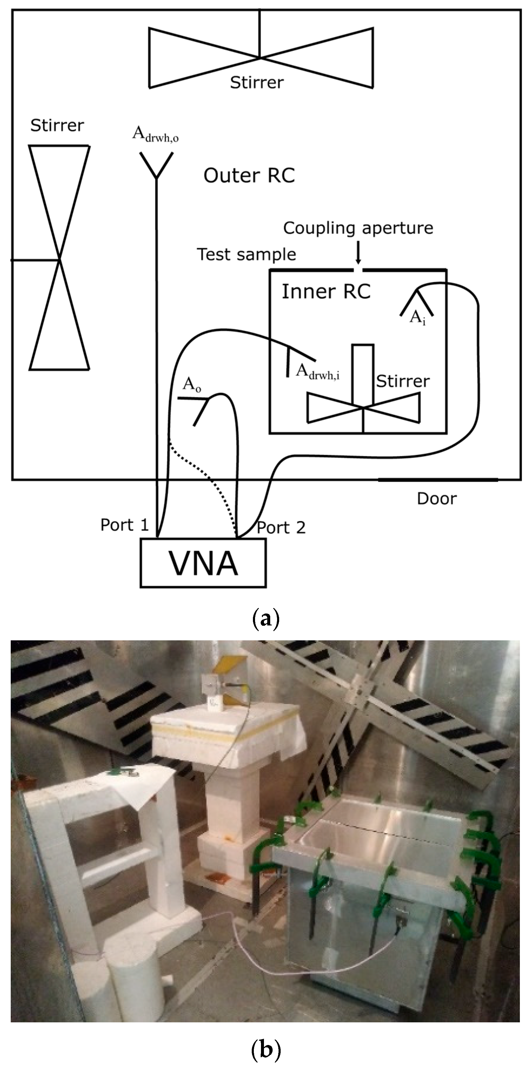
Figure 1a shows a sketch of the measurement setup, including the nested RCs [
5], and
Figure 1b shows the inside of the RC, where the inner chamber is visible. The RC has three stirrers, which work in continuous mode. The inner sizes of the inner chamber are exactly 473 mm × 473 mm × 473 mm. It has a removable side, which is exploited to change the coupling configuration. The removable side was positioned on the flange of a width of 40 mm of the inner chamber. The apertures were created by cutting off parts of aluminum slabs, which were used as removable sides. These interchangeable aluminum slabs were properly placed on the flange of the inner chamber, which was covered by a sealing gasket. An efficient homemade stirrer was used to achieve an acceptable assumed field distribution inside the inner chamber. The stirrer, which works in continuous mode, includes a vertical prism, metalized by adhesive aluminum except for the top wall. The measurement setup is the same as that used in [
5]. The scattering parameters S
21,o,i, S
21,o,o, and S
21,i,i, which are the transmission coefficient between the chambers and those of the outer and inner chambers, respectively, are measured. It is specified that the subscript
o (
i) means outer (inner) chamber. Such subscripts could be replaced with subscripts
1 (
2) when any system of CRCs is considered, such as two adjacent RCs. It is also specified that the coefficients S
21,o,i and S
21,i,o are the same for the reciprocity. The former coefficient (S
21,o,i) refers to the case in which the transmitting antennas are placed inside the outer chamber, and the receiving one is placed inside the inner chamber; the latter coefficient (S
21,i,o) refers to the case in which the transmitting antennas is placed inside the inner chamber and the receiving one is placed inside the outer chamber. The measurements of the coefficients are performed over the frequency range (FR) from 1 GHz to 18 GHz.
The antennas used in the experiments are a couple of ETS-Lindgren 3115 double-ridge waveguide horn antennas, of which one is placed in the outer chamber and the other is placed inside the inner chamber. The other two antennas are ultra-wideband image transmission TEM antennas (model XR 170), which are Vivaldi-type antennas; manufacturer: Shenzhenshi Desheng Wangluo Keji Youxian Gongsi; Shenzhen, China. The measurement setup includes a two-port Agilent 8363B vector network analyzer (VNA); manufacturer: Agilent Technologies; Bayan Lepas Free Industrial zone, Penang, Malaysia.
In the measurements, 1700 uniformly distributed uncorrelated samples over the whole FR from 1 GHz to 18 GHz were gathered for each frequency sweep. Fifty frequency sweeps were acquired for each of the three measured scattering parameters. A step frequency of 10 MHz was used. In short, 50 uncorrelated samples were acquired for each of the 1700 frequency points. The possible biases of the real and imaginary parts were removed frequency by frequency. Consequently, the samples to be processed were also independent. Hence, we obtained and tested 1700 CDFs, each derived from 50 measured samples of the amplitudes of the parameters , , and , using the p-value from the Anderson–Darling (A-D) test.
4.2. Results from Measurements Using Two Canonical Cases of Single ESCAs
The two ESCAs used in the measurements were a rectangular slot shape of 20 mm × 2 mm for the 1D case and a circular hole shape of 16 mm in diameter for the 2D case. For these small coupling apertures, the assumption of independence of the fields inside the two coupling chambers can be clearly assumed, as shown below.
First, results from the two chambers when they operate in a standalone way are shown, in order to verify the assumed distribution inside the single chambers. Only the distributions of the field components are considered in the statistical tests for brevity. On the other hand, the distributions of the powers were used to corroborate theoretical results.
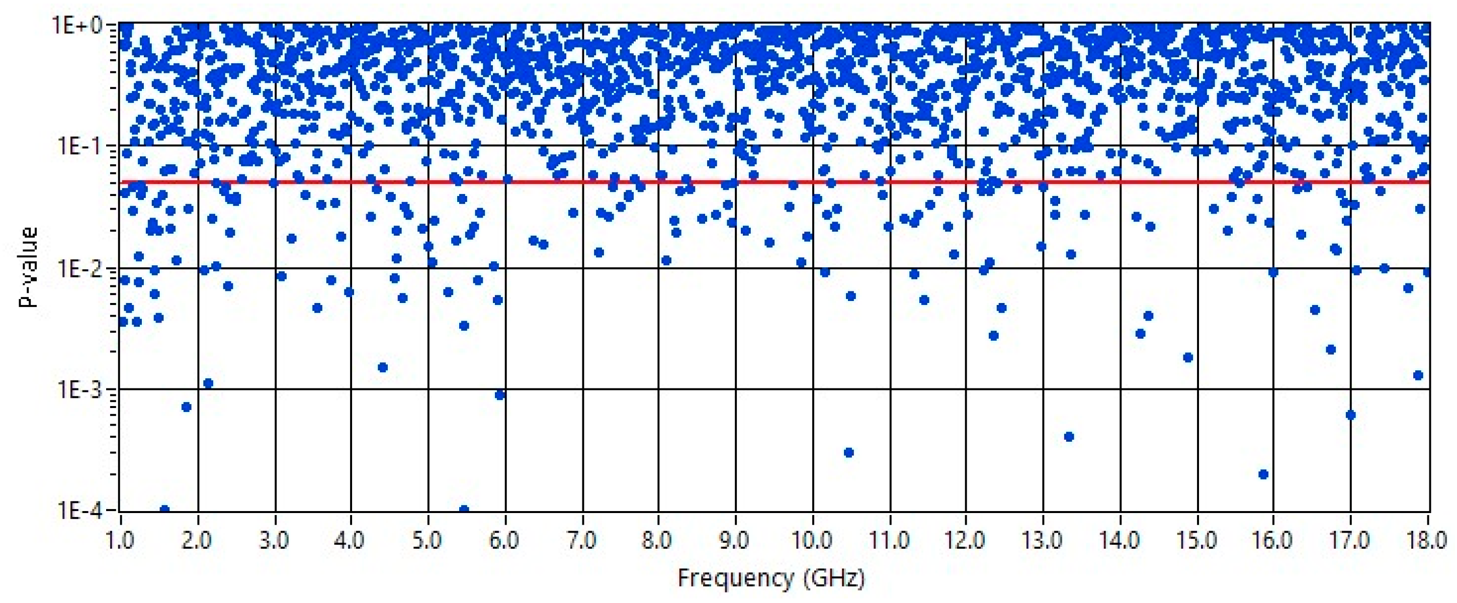
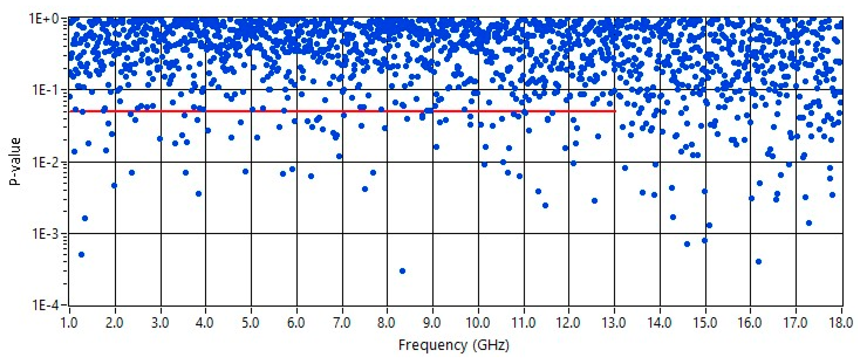
Figure 2 and
Figure 3 show the
p-value for the nonnormalized amplitude of S
21 measured inside the inner chamber and inside the outer chamber, respectively. In these measurements, the inner chamber was inside the outer chamber, and the coupling aperture was 32 mm × 2 mm. In these two cases (outer and inner chamber), the theoretical CDF is a χ distribution with 2 DOF.
For the inner chamber (
Figure 2), the theoretical hypothesis was rejected at 5% and 1% significance levels; the rejection rates were 10.2% and 2.9%, respectively. Note that the red line represents the threshold at the 5% significance level. The rejection of the test on the distribution of the amplitude of the field components inside the inner chamber was likely because of an ordinary imperfect stirring inside the inner chamber, which was due to the limited volume and only to the use of MS. Such an imperfection was rather generalized over the entire FR even though it was more significant at the lower frequencies, where the modal density is lower, as expected [
5].
However, the map of the p-values and the rates of rejection of the test show that the results are acceptable for the sake of comparison in this paper.
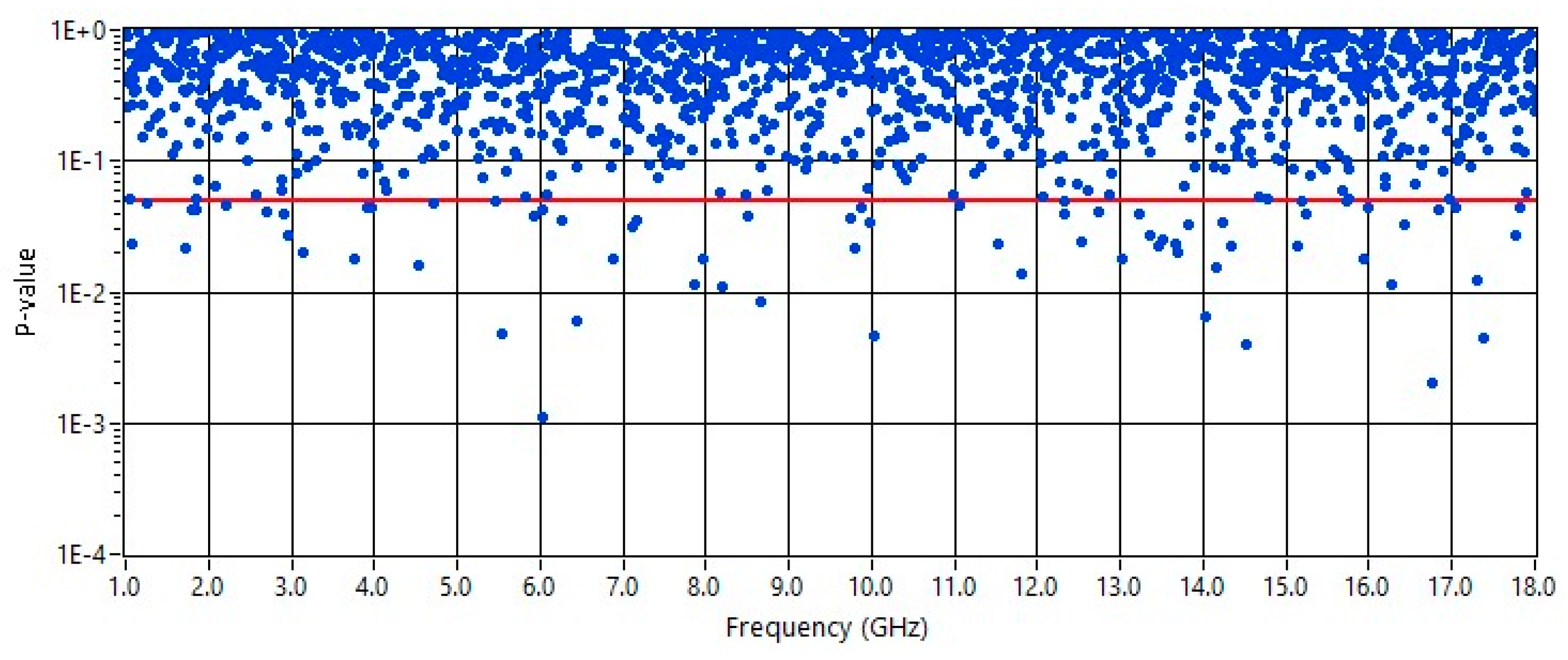
For the outer chamber (
Figure 3), the theoretical hypothesis was accepted both at the 5% and 1% significance levels, as expected. In this case, the rejection rates were 4.0% and 0.5%, respectively.
The results shown in
Figure 2 and
Figure 3 are perfectly consistent with the corresponding ones presented in [
5], as expected.
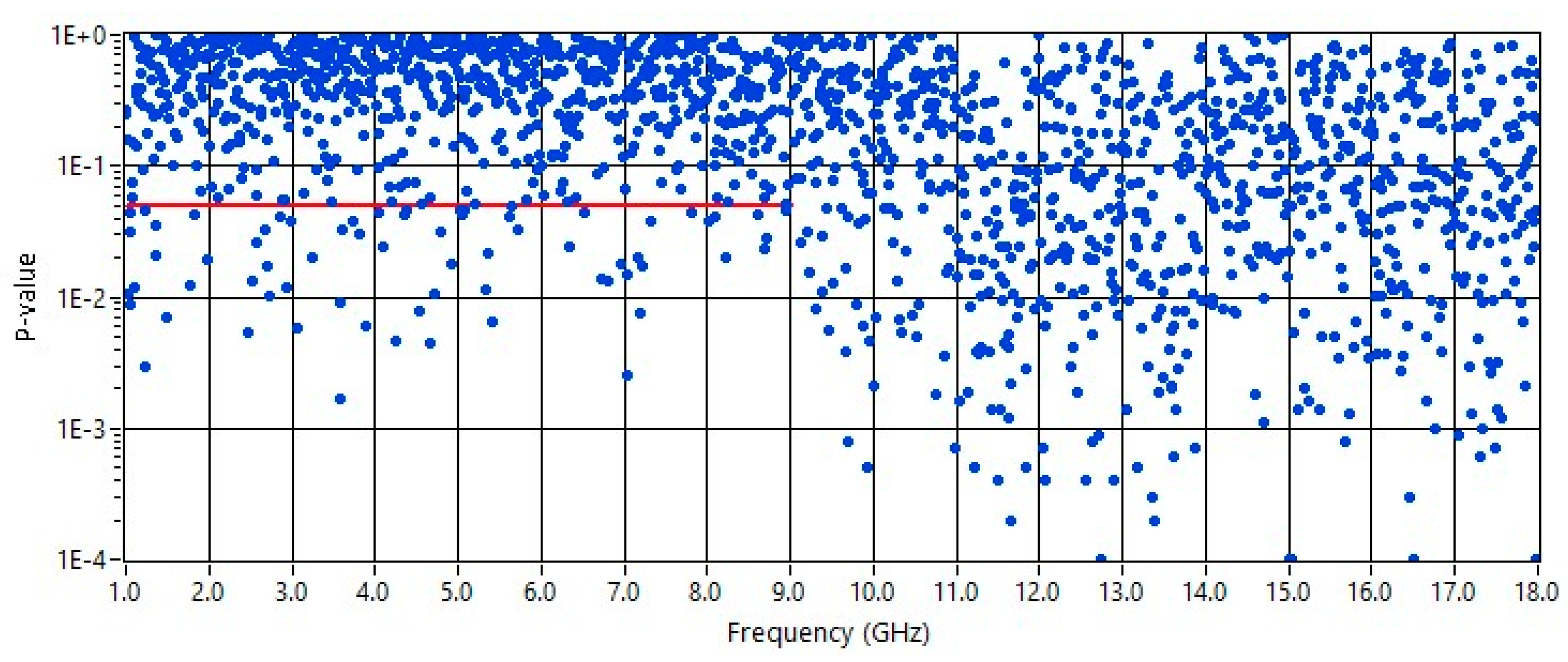
Figure 4 and
Figure 5 show the results of the
p-value for the nonnormalized amplitude of S
21,o,i, measured between the chambers, in the case where the coupling apertures were the slots of 20 mm × 2 mm and the hole of 16 mm in diameter, respectively. In
Figure 4, the theoretical hypothesis is the nonnormalized double Rayleigh, i.e., the CDF expressed by Equation (2). In
Figure 5, the theoretical hypothesis is the CDF expressed by Equation (6).
The cut-off frequency of the slot of 20 mm (
Figure 4) is 7.5 GHz. However, the A-D test was performed over the sub-FR from 1 GHz to 9 GHz for the nonnormalized double Rayleigh distribution. The theoretical hypothesis was rejected at the 5% and 1% significance levels; the rejection rates were 8.4% and 1.7%, respectively. We note that the rejection rates strongly worsen for frequencies from 9 GHz to 18 GHz.
The cut-off frequency of the circular hole of 16 mm in diameter is about 11 GHz. However, the A-D test was performed over the sub-FR from 1 GHz to 13 GHz. The theoretical hypothesis was rejected at the 5% and 1% significance levels; the rejection rates were 5.5% and 1.7%, respectively.
We specify that the tests in this paper were performed up to more than the cut-off frequency of the coupling aperture, as the results were reasonable and acceptable up to about the considered frequencies.
Note that the rejection rates in
Figure 4 and
Figure 5 are totally compatible with those due to imperfect stirring inside the inner chamber (see
Figure 2 and
Figure 3). Therefore, even though the test was rejected at 5% and 1% significance levels for these apertures, the rejection ratios and the
p-value maps show that the experimental and theoretical CDFs match well. Moreover, the visible migration toward a different distribution is also expected for the electromagnetic behavior of the two apertures, which de facto represents the real physical problem [
5]. Indeed, the distribution of the field components inside the inner chamber changes from ES to EL by crossing the resonance region, according to the ratio between the size of the apertures and the wavelength over the FR. In other words, the coupling apertures can be considered “electrically small” until the frequencies in the resonance region of the aperture itself, where the amplitude and phase of the field on the aperture still can be considered approximately constant. It is specified that the transitional behavior from ES to EL aperture is shown for a circular aperture (2D case) in ([
5], Figure 11), where normalized CDFs were considered.
Again, the results shown in
Figure 4 and
Figure 5 are perfectly consistent to the corresponding ones presented in [
5], as expected.
4.3. Results from Measurements Using Two Electrically Large Canonical Apertures
In [
3], the experiments are not systematically designed in the case of ELCAs. Furthermore, the condition of sufficient isolation between the coupled chambers is not fully considered, as the results ([
3], Figures 4 and 5d) reflect. In [
15], the isolation between the chambers is sufficient; however, the results and comments are in contrast with the theory in [
4], as mentioned in [
5]. It is important to note that the theory regarding ELCAs, which is discussed in [
4], is simple and robust. The assumption of the independence of the fields in both chambers entails that the chambers are sufficiently isolated so that the multiple interactions between the chambers are negligible, as shown in [
16,
17,
18]. In [
16], a sufficient condition is given for such an isolation. It is important to note that if the CA is not electrically small and or the chambers are not sufficiently isolated, the distributions of the field components and the associated powers inside the chamber fed by the other one move towards the χ distribution with two DoF and the χ-squared distribution with two DoF, respectively [
5], according to the size of the CA and or of the isolation level. Such distributions are obvious and well-known for fields and powers inside the two chambers when they are considerably coupled. Therefore, it is relevant to show the distributions of fields and powers in cases where the CAs are electrically large and at the same time the two chambers are sufficiently isolated according to an objective measure.
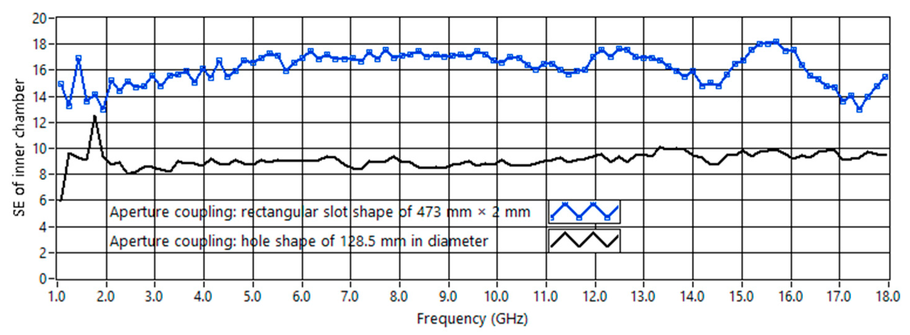
The two ELCAs used in the experiments have a rectangular slot shape of 473 mm × 2 mm and a circular hole shape of 128.5 mm in diameter, for which the first case acts as a 1D ELCA and the second case reflects the behavior of a 2D ELCA similar to those used for shielding effectiveness (SE) tests of materials and gaskets [
17].
In this case, the expected distribution of the amplitude of the field components is a χ distribution with two DoF.
Figure 6 shows the SE of the inner chamber for both the ELCAs mentioned above; it is obtained by measurements. The SE of the inner chamber is obtained by evaluating the expression
, where the subscripts
M and
F are the number of samples from mechanical stirring and the number from frequency stirring; that is, such averages are obtained by using both mechanical stirring and frequency stirring. It is specified that in our case,
M = 50, which is the same as the acquired frequency sweeps, and
F = 17; the latter is deliberately chosen to be a submultiple of 1700, which is the number of samples over the whole FR from 1 GHz to 18 GHz as mentioned above. The total number of samples to obtain the averages for SE is
N = 50 × 17 = 850. The frequency stirring bandwidth is equal to (17 − 1) × 10
6 = 160 MHz.
We note that the SE is greater than or equal to 5 dB; therefore, the assumed isolation conditions are met [
16,
17,
18]. Note that SE ≥ 5 dB is a sufficient condition for the isolation of the two coupled chambers [
16,
17,
18]. In other words, the fields inside the two chambers can be considered as independent for the two cases of ELCAs presented in this work. If SE is greater than or equal to 5 dB, the chamber isolation
is greater than or equal to 10 dB [
19], and consequently, the multiple reflections between the two chambers can be neglected [
16]. In other words, the reflection of the energy from the feed chamber towards the feeding one can be neglected; the coupling between the chambers turns out to be weak enough to consider the corresponding volumes as separate. Considering also that the fields are independently stirred in both chambers and that the losses inside the chambers are independent of each other, the independence of the fluctuations and of the distributions of the fields inside the chambers can reasonably be assumed. It is important to note that if the sufficient condition for the isolation (SE ≥ 5 dB) is met, the isolation between the two chambers is always greater than 10 dB; indeed, it turns out to be equal to 10 dB only for two chambers, for which
. It likely could occur for two adjacent and equal chambers (here the concept of “equal chambers” includes volumes and related inner total losses, so that it turns out to be
). We also note that the SE of the inner chamber is greater than the value in ([
17], Figure 16), because the inner chamber was loaded in the measurements performed in this paper, as it is visible in ([
5], Figure 4a). It is specified that the SE of an enclosure depends both on the SE of the wall material [
20] and the total inner losses, which include losses in the walls [
21].
It is specified that the distribution of the field components in the inner chamber was, however, tested in the case of the circular hole shape of 128.5 mm in diameter, when it operates in a standalone way, to check the assumed distribution of the fields. The results closely resemble those presented in
Figure 2 and are therefore omitted for the sake of brevity.
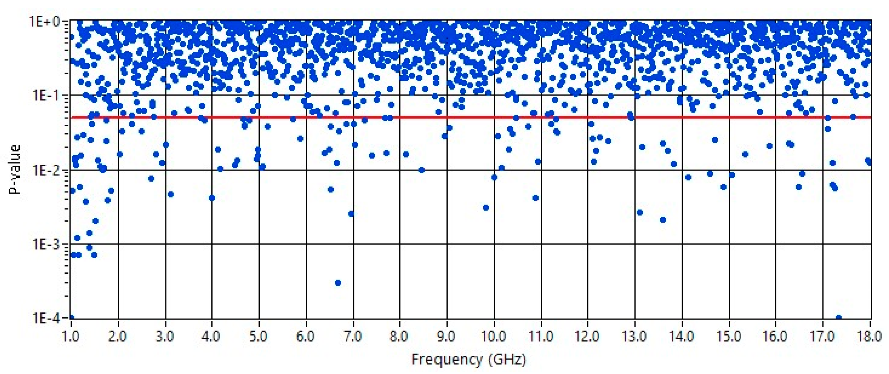
Figure 7 shows the results of the
p-values from the comparison between theoretical and experimental CDFs, where the former is a nonnormalized χ distribution with 2 DoF, whereas the latter is obtained by the measured amplitudes of S
21,o,i, in the case where the CA is a slot of 473 mm × 2 mm. The theoretical hypothesis is rejected at the 5% and 1% significance levels over the whole FR; the rejection rates are 7.4% and 2.2%, respectively. It is important to note that the rejection rates in
Figure 7 is completely compatible with those due to imperfect stirring inside the inner chamber as mentioned above. Therefore, even though the test was rejected at the 5% and 1% significance levels for these apertures, the rejection ratios and the
p-value maps show that the experimental and theoretical CDFs match well. The red line represents the threshold at the 5% significance level.
Figure 8 shows the results of the
p-value from the comparison between theoretical and experimental CDFs, where the former is a nonnormalized χ distribution with 2 DoF, whereas the latter is obtained by the measured amplitudes of S
21,o,i; the CA is a hole of 128.5 mm in diameter.
The theoretical hypothesis is rejected at the 5% and 1% significance levels over the whole FR; the rejection rates are 6.6% and 1.8%, respectively. Again, it is important to note that the rejection rates in
Figure 4 is completely compatible with those due to ordinary imperfect stirring inside the inner chamber. Therefore, even though the test was rejected at the 5% and 1% significance levels for these apertures, the rejection ratios and the
p-value maps show that the experimental and theoretical CDFs match well. From
Figure 7 and
Figure 8, we note a reduction in the
p-value at low frequencies, specifically over the sub-FR from 1 GHz to 2 GHz. It is likely due to the effect of two independent causes: the size of the CA and volume of the inner chamber, as discussed in [
5].
5. Conclusions and Discussion
In this work, the PDFs and CDFs of the nonnormalized field components and nonnormalized related powers inside CRCs were derived, from which we easily achieved corresponding normalized statistics for both field components and related powers. Two cases of single electrically small CAs were considered. These two cases involve one-dimensional (1D) and two-dimensional (2D) single electrically small CAs, respectively. We showed that the accuracy of the theoretical distributions can be validated by the comparison between the MSVs of the nonnormalized PDFs of the field components and the MVs of the nonnormalized PDFs of the corresponding received powers, when they are achieved in an independent way and hence on a physical basis. The theoretical results were also supported by the comparisons with the results from measurements.
Moreover, we showed two canonical cases of the results from measurements using two ELCAs: a rectangular slot shape of 473 mm × 2 mm and a circular hole shape of 128.5 mm in diameter.
It is important to note that the rationale used to achieve the theoretical and experimental results presented in this paper can also be used for a chain of coupled enclosures. It is highlighted that results expressed by Equations (5)–(8) are totally novel, and they are very useful to achieve statistical models for predicting distributions of fields and powers in coupled enclosures, also when the coupled cavities are more than two, as in [
7]. In other words, we can easily study the distributions of fields and powers inside the third, fourth, etc., of a chain of N coupled enclosures in cases where they are coupled by a single ESCA, by an ELCA, or by many apertures and are sufficiently isolated.
This study is useful and applicable in electromagnetic compatibility, both for radiated emissions and radiated susceptibility [
22], as well as SE measurements, where the statistics of fields and powers inside coupled cavities are involved. They are useful for both internal and external interferences due to radiated electromagnetic emissions [
22], where the knowledge of the statistics of fields and powers inside coupled cavities allows us to accurately know the probability of values of fields and associated powers above a certain threshold value [
1]. For SE measurements, the knowledge of the statistics of fields and powers allows us to select the measurement model more appropriate to improve the accuracy [
1,
17]. In short, for these applications, the distributions achieved can be considered as a reference for coupled enclosures in the real world.
Finally, in addition to coming up with new results, this study provides a systematic organization of the field and power distributions for coupled enclosures.


