Surface Resistivity Imaging for Drilling Columnar Cores

Abstract

The resistivity imaging system is specifically designed for the precise measurement of resistivity distributions within drilled columnar core samples. Its coaxial symmetric configuration enables the non-destructive characterization of electrical properties, with broad applications in oil and gas exploration, reservoir evaluation, and geological research. By integrating a ring return electrode and full-circumference electrode arrays, the system can acquire core-scale resistivity data in conductive media environments. The self-developed imaging software employs advanced processing algorithms—including depth correction, amplitude normalization, and image enhancement—to transform raw resistivity measurements into high-resolution surface imaging maps. Experimental results demonstrate that the system can resolve features such as cracks with a minimum width of 0.5 mm and pores with a minimum inner diameter of 0.4 mm in granite core, providing a novel technical approach for the fine-scale characterization of core materials.

1. Introduction

A core is a cylindrical rock sample extracted from a borehole using a ring-core drill bit and other coring tools, in accordance with the requirements of geological survey work or engineering projects. It offers the possibility to directly observe geological conditions and serves as a crucial link facilitating the exchange of information between the surface and the subsurface. Through in-depth analysis of the core, we can not only directly ascertain the rock type and the physical and chemical properties of the formation (such as permeability [1,2], saturation [3,4], pore characteristics [5,6,7]), but also furnish first-hand information for evaluating reservoir characteristics, identifying source rocks and cap rocks [8,9]. Moreover, when integrated with other geophysical data, core data can remarkably enhance our understanding of subsurface geological models, thus increasing the overall success rate of the project [10].

Rock materials can be recognized based on scanning electron microscopy (SEM) images [11]. However, the SEM image can cover the size of several microns, and it is not valid for drilled cores. Measuring the resistivity of the core is the primary approach for characterizing reservoirs. The electrical resistivity can be measured by a direct current (DC) or alternating current (AC). The electrodes can be placed on the surface of the specimen, positioning an electrode disk or a linear array, or by a four-probe square array [12,13,14]. An automated/semiautomated digital multi-electrode instrument was designed with direct current electrical (geoelectric) methods [15]. Some researchers created conductive materials capable of monitoring the behavior of concrete structures [16]. Cracks can be obtained with embedded electrodes [17]. A mini-electric imaging survey with a Wenner array was conducted, and the development of cracks was monitored [18]. Saturated rocks were applied with multiple electrical voltage measurements. A crack in a fractured core sample can be recognized in the resistivity scan; however, the resolution is limited to between 0.5 and 0.75 mm [19].

In this paper, we present our self-developed core resistivity imaging setup. The shielding electrode and stainless-steel electrode array are placed in the coaxial symmetric system, which can help achieve non-destructive detection of the electrical characteristics. The resistivity distribution for drilled columnar cores like sandstone, granite, and other rocks can be obtained in a conductive environment simulating the underground magma. The cracks and pores can be recognized in the resistivity image of the core. The distribution, development patterns, and physical properties of cracks and pores may indicate the potential for carbonate reservoir exploration and development.

2. Setups and Methods

2.1. Surface Resistivity Imaging System

As shown in Figure 1, the core resistivity imaging system consists of the following main components. A polypropylene (PP) tank is employed to hold the electrolyte prepared from a 15% concentration of NaCl solution. The volume of the prepared electrolyte is determined by the length of the core to be tested, and the electrolyte must submerge the circular return electrode to ensure that the entire device is within the same current path. The electrolyte is configured so that no other metal conductors are present; only the components of the core are placed in it, and there is no current loop in the electrolyte other than the one surrounding the core itself.

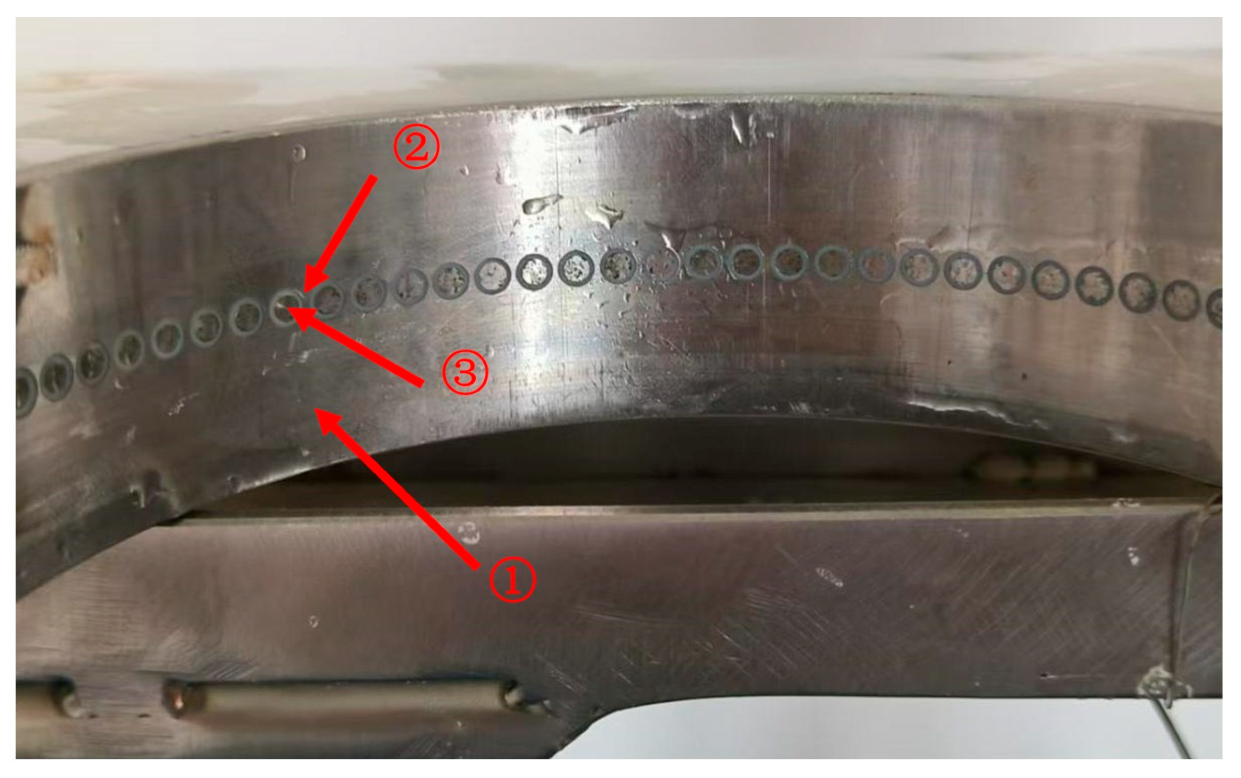
The Φ105 mm core holder is made of naval stainless steel, which can be placed in the electrolyte for an extended period and can meet the requirements of multiple scanning measurements. The clamping method is a Hassler-type core holder, which is currently the most commonly used in core analysis. It is characterized by ease of use, convenient loading and unloading of rock samples without having to dismantle the entire core holder. Its structure comprises two semicircular hollow structures with an inner diameter of Φ105 mm. The core clamping device adopts the method of applying radial pressure on the column surface of the core to seal the side wall of the core. With the assistance of flexible plastic shrapnel, it can expand the adaptability range from Φ103 mm to Φ105 mm of the core clamping device.

Currently, the core resistivity imaging system employs a perimeter array of circular buckles, which are arranged in a single, densely packed row. Circular reflux electrodes are positioned at the perimeter of the buckle array (⑤ in Figure 1), directly above the core. The perimeter of the buckle array and the circular reflux electrode are coaxial and are fixed within the auto-stepper robot arm. They are controlled by the auto-stepper robot arm (⑦ in Figure 1) to move vertically along the vertical direction.

The automatic stepper arm is made of naval brass, which has strong corrosion resistance and good rigidity. It is not prone to deformation during the movement of the arm, thus reducing the possibility of errors in the testing process. The automatic stepping motor is selected CL-01A (Haijie Technology, Beijing, China). It is characterized by single-axis operation and is arbitrarily programmable (capable of realizing a variety of complex operations: positioning control and non-positioning control). It has a maximum output frequency of 50 kHz, a resolution of 1 Hz, and a minimum displacement step of 0.01 mm, which is also the minimum measurement accuracy of this core measuring device.

As shown in Figure 2, the pole plate is equipped with an array of button electrodes and shielding electrodes. The stainless-steel button electrodes (③ in Figure 2) and stainless-steel shielding electrodes (① in Figure 2) are separated by the insulating material polytetrafluoroethylene (PTFE), and the return electrode is designed as a ring directly above the pole plate. Both the button electrode and the shielding electrode output alternating current (AC) signals with the same potential, frequency, amplitude, and phase. The same AC signals on button electrodes and the shielding electrode can help avoid current flows directly through the electrolyte solution outside the core. The current from each button electrode can flow nearby the electrode and the core, then to the circular reflux electrodes (⑥ in Figure 2)

The diameter of a standard core is D mm, and the diameter of the plate is D + X mm (where X ranges from 0.1 to 3.0 mm). The core resistance imaging device uses shielded wires to connect the circuit module to each button electrode on the pole plate. These shielded wires are used to transmit test signals and prevent interference from inter-electrode AC signals. To maintain a tight fit between the core and the plate and keep the core level with the plate, it is essential to ensure the core is upright and not tilted. A rigid spring is used to apply an external force to the plate to keep it locked. The core clamping device at the bottom is made of an elastic material, and its size is determined by the diameter of a standard core D. The return electrode (a stainless-steel ring) of the core resistance imaging device is located directly above the pole plate, and its vertical distance from the pole plate is selected as 3 cm, which yields a better imaging effect.

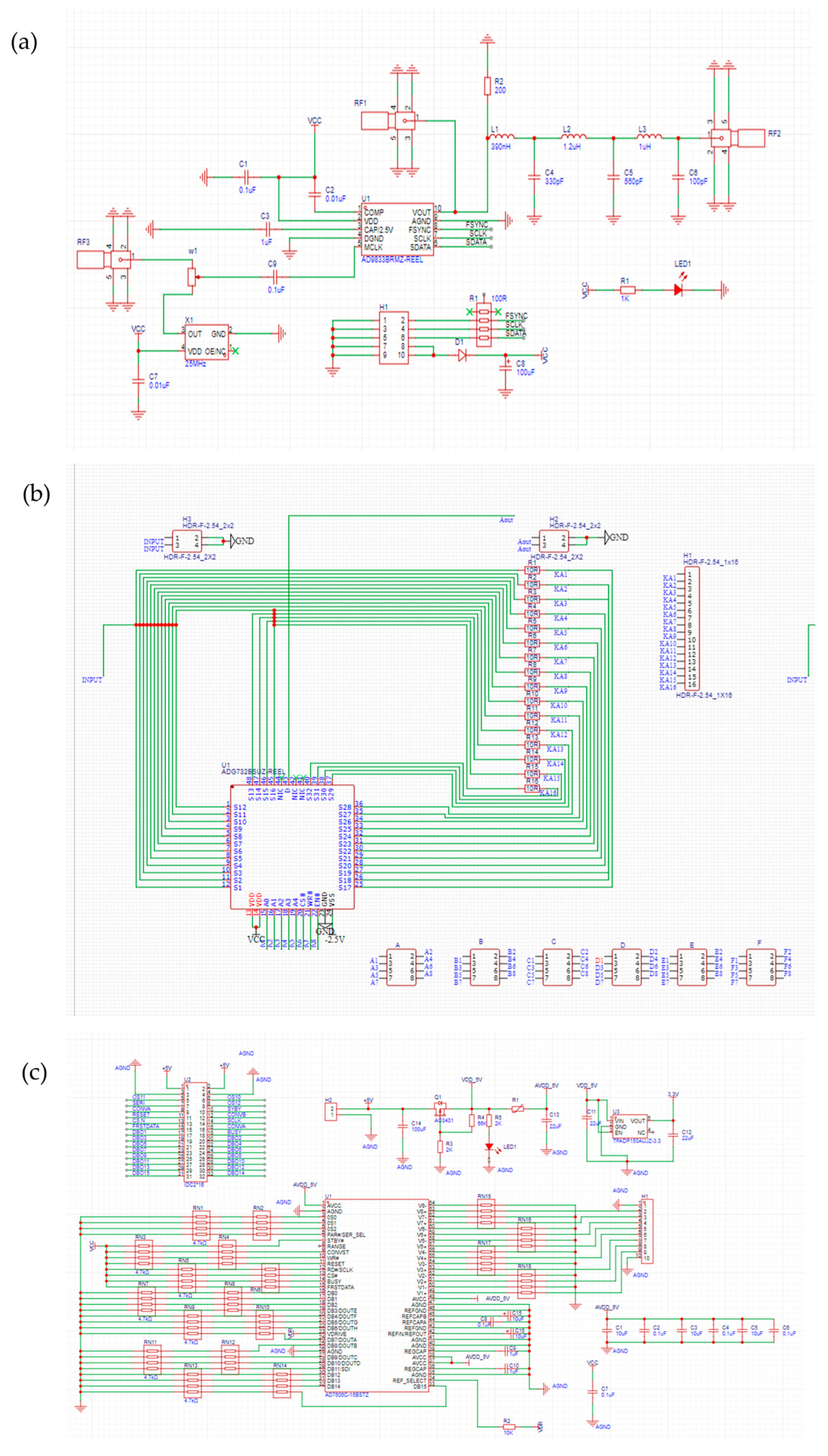
The circuits for the core resistivity imaging system are composed of a signal generation module, switching module, and signal acquisition module, as shown in Figure 3. The signal generation module enables precise control of frequency, phase, and waveform. By integrating a high-current operational amplifier into a dynamic gain amplification chain, and combining a dual-buffer mechanism, multi-stage filtering, and closed-loop calibration, it can achieve stable signal output across a wide range. An 88-channel sensor signal selection network is established in the switching module. Through timing control, crosstalk between channels is ensured to be <−80 dB. Together with an instrumentation amplifier (with adaptive gain adjustment) and a negative voltage generation module, it realizes signal enhancement and noise suppression. Self-calibration firmware is incorporated (channel consistency error < 0.1%). The signal acquisition module can achieve synchronous acquisition of 88-channel differential signals. Through precise timing control by an FPGA and USB dual-buffer transmission, combined with real-time processing and multi-stage calibration (hardware self-calibration + software calibration, linearity error < 0.02%), it enables high-precision resistivity imaging.

The system ensures long-term stable operation in complex electromagnetic environments and high-load conditions through wide-range signal coverage, redundant power supply design, thermal management, and anti-interference measures, providing reliable technical support for the measurement of core electrical characteristics.

The transmitting voltage of the core resistive imaging device is provided by the signal generator module, which is controlled by DDS. The AC voltage signal is connected to a voltage amplifier for adjustable output. The output voltage amplitude V ranges from 0.1 to 10 V, and the frequency K ranges from 100 to 20 kHz.

The voltage magnitude at the corresponding position of the rock core is collected by the button electrode. A sampling resistor is placed between the button electrode and the emitting resistor. The resistance value of the sampling resistor R can vary from 1 Ω to 1 KΩ. The voltage V on the sampling resistor is taken out by the differential toggle switching circuit, filtered, and amplified by the differential amplifying circuit, which can amplify tiny signals and send them to the data acquisition system.

The switching module and data acquisition module operate in sequence. The core resistance imaging device has an array of N button electrodes with a diameter of d (ranging from 0.2 mm to 10 mm) distributed along the inner side of the pole plate in a circular pattern. The pole plate locking device of the core resistance imaging device applies force to the pole plate through the elastic element, causing the pole plate to close the inner circle. This ensures effective electrical conduction between the pole plate and the core to be measured while avoiding direct contact.

The pole plate of the core resistive imaging device is connected to a control automatic stepping motor. Parameters of the control automatic stepping motor, such as the step length h, the number of steps p, and the dwell time t at a single depth point, are set on the computer side for automated core measurement.

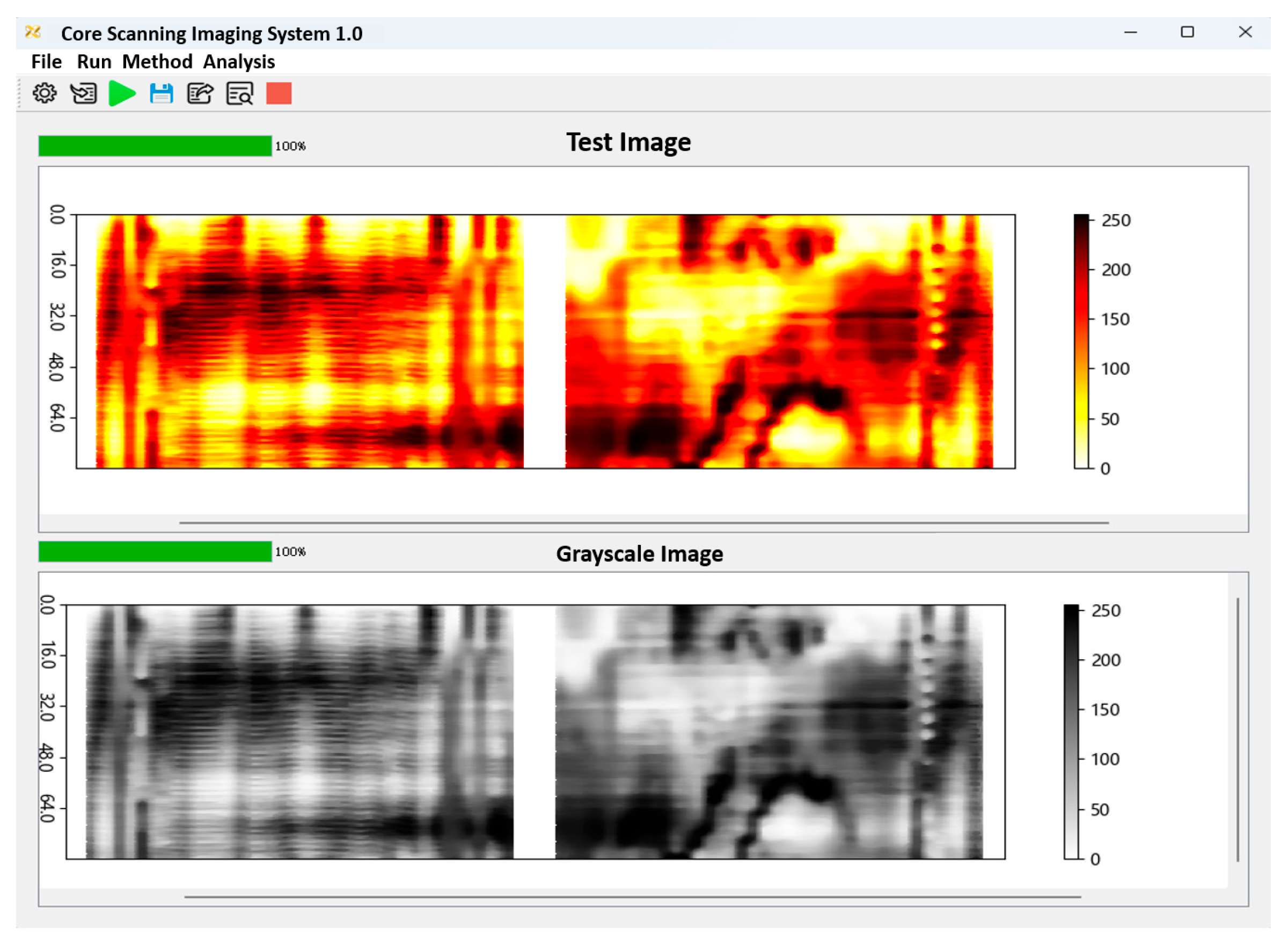
The imaging of the core resistive imaging device is carried out by software that is specifically matched to the imaging device. This software incorporates algorithms designed to generate images from the stored data. The images are exported in the form of coordinates (X, Z). Here, the X-axis represents the data obtained from different button electrodes at the same depth point m, while the Z-axis represents the data from different depth points corresponding to the same button electrode i. The data of the same button electrode i at different depth points are also exported in the form of (X, Z). The coordinates are determined by the following equation:

$$X\left(i\right)=\pi D/N\times i$$

(1)

where i is the corresponding button electrode, i ∈ (0, N − 1).

$$Z\left(m\right)=H0+h\times m$$

(2)

where m is the corresponding depth point, m ∈ (0, p − 1), H0 is the starting measurement position, and the distance tested is H = h × p.

$$R(X,Z)={\displaystyle \frac{V-v(X,Z)}{v(X,Z)/R}}$$

(3)

where V is the output voltage of the signal generator, v (X, Z) is the voltage value on the sampling resistor corresponding to the button electrode at lateral position X and depth Z, and R is the resistance value of the sampling resistor.

The core resistive imaging device uses algorithms such as equalization processing, error correction, and other algorithms to process the image during imaging.

The data acquisition system of the core resistivity imaging system is connected via a USB serial port, boasting a sampling frequency of up to 200 kHz. Based on the Nyquist sampling theorem, the sampling frequency should be at least twice the signal frequency. The maximum range of the data acquisition system is ±10 V.

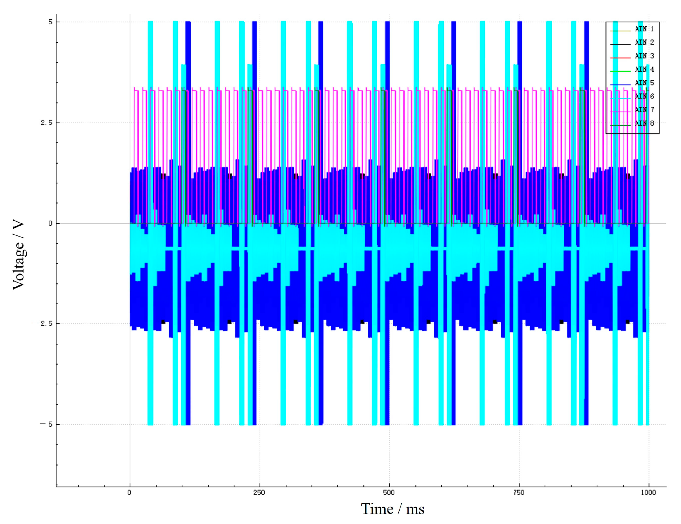
This data acquisition system employs six channels for parallel acquisition. Each channel encompasses 16 button electrodes on the full-perimeter button array. Consequently, the real-time voltage value on each button electrode can be observed in the data acquisition panel as shown in Figure 4. The voltage magnitude corresponds to the voltage magnitude of the core at the corresponding position at that instant, from which the resistance value at the corresponding position can be deduced. After data acquisition, the data is stored as a csv-format file. The file size is determined by the length of the tested core and the sampling frequency. Specifically, the longer the length of the tested core and the higher the sampling frequency, the larger the file size will be, and the longer it will take for the program to process the image.

2.2. Methods of Core Resistivity Imaging

To guarantee the accuracy of subsequent processing during the imaging process, the measurement data must be appropriately pre-processed. The crucial steps in the pre-processing of core resistivity measurements comprise depth correction (including coplanar correction, acceleration correction, etc.), amplitude correction (such as EMEX voltage correction, data normalization, bad snap correction, and equalization correction, etc.), and image enhancement [20,21]. As shown in the flowchart of Figure 5, once the pre-processing is completed, the imaging of the processed data is carried out.

(1)

Depth correction

① Coplanar correction

When there are irregularities in the core, the tension angles of the individual plates in contact with the core sidewalls will vary. This leads to a vertical depth misalignment among them, which needs to be rectified to a coplanar state by integrating the characteristics of the core wall and the instrument structure. The vertical displacement caused by differences in the instrument tension angles is calculated as follows:

$$H\left[i\right]=ArmLen - sqrt(ArmLen\ast ArmLen-(c\left[i\right]-PtLen)\ast (c\left[i\right]-PtLen\left)\right)$$

(4)

where \(H[i]\) represents the vertical displacement of the plate, \(ArmLen\) is the arm length of the plate, \(c[i]\) is the radius of the corresponding core part of the plate, and \(PtLen\) is the thickness of the plate.

② Acceleration correction

During the measurement process, if the instrument moves non-uniformly, or even gets stuck or unstuck, the acquired data will show image stretching and compression, as well as jagged misalignment between the polar plates after time–depth conversion. It is necessary to combine the operating state of the instrument to restore the data to an isochronous state of uniform sampling according to the depth. Through resampling, some missing details can be recovered, and the misalignment between the polar plates can be rectified. However, it is impossible to reconstruct the severely missed measurements caused by significant jamming.

(2)

Amplitude correction

① EMEX voltage correction

To ensure that the instrument can effectively sample the core surface within its own dynamic range during the measurement (without zeroing or saturation), the transmitter voltage of the acquisition circuitry is automatically adjusted to control the measured current strength. This ensures that the measured current can effectively penetrate the formation and form the measurement loop. Therefore, in the vertical direction, amplitude uniformity is required to enhance the vertical stratigraphic comparability. The general formula for EMEX voltage correction is as follows:

$$pArray \left[ip\right] \left[ilg\right] \left[idm\right]\ast ={\displaystyle \frac{EmMx}{pEmex}}\left[ip\right]$$

(5)

where \(EmMx\) represents the global maximum of the EMEX voltage, \(pEmex[ip]\) is the read value of the EMEX voltage at each depth point, \(pArray\) is a 3D cache array of the imaged logging data, and \(ip\), \(ilg\), and \(idm\) represent the serial number indices of its depth, pole plate, and electrode buckle, respectively. Meanwhile, \(ipk\) is the difference in depth (number of samples) of the electrode buckles with respect to the standard logging point, and the same notation applies hereinafter.

② Bad Buckle Correction

For individual electrical buckles with abnormal statuses, the measurement curve shows flat or jumped values. These can be detected by statistical techniques and repaired through interpolation. In the case of the jump-value phenomenon, the procedural processing requires the use of median filtering. Since both the statistical detection and filtering repair computations are relatively intensive, the manual repair of abnormal segments through manual observation is generally considered. For the automatic repair of bad buckles, this study is implemented as follows: first, the variance of each specified buckle curve is calculated and compared with the in-window variance of all buckle curves. If this variance is greater than a certain cut-off value (specified by the user), it is identified as a dead buckle, which is generally repaired by interpolating the average value of the neighboring buckles.

③ Data Normalization

The degrees of attachment of the buckles to the well wall and the electrode coefficients vary, resulting in different measured background values between buckles, and the images do not have a consistent background color. The logging data must be normalized to ensure that the measured data from each buckle has consistent mathematical and statistical expectations.

During the measurement process of the resistivity imaging logger, the contact degrees between each pole plate and the well wall cannot be exactly the same; some may have better contact while some may have worse contact. For the electric buckles on the same pole plate, their electric buckling coefficients may not be identical, and their contact degrees with the well wall may also differ. Due to the influence of the above-mentioned factors, there may be some differences in the logging responses of each buckle to a formation with the same resistance value. This leads to the absence of a consistent background color between the buckles on the image, which is an unavoidable drawback in the instrument design and needs to be addressed in data processing.

For a particular measurement well section, the measured values of each electric buckle should be basically the same, meaning there should be a certain mathematical expectation. Additionally, the distribution of its measured-value data should basically follow a normal distribution. This provides the possibility to improve the borehole resistivity imaging image through mathematical methods. There are numerous data-normalization methods, such as data standardization, data regularization, extreme-value normalization, mean-value normalization, standard normalization, and centering. After the data-normalization process, the image resolution between the polar plates of the resistivity imager can be significantly improved, and the background values of the polar plates can be ensured to be consistent, thereby enhancing the visual effect.

④ Equalization Correction

During the measurement process, due to the differences in the contact degrees between each pole plate and the core sidewall, the differences in the sensitivity/signal gain of the buckles, the non-homogeneity of the core conditions in all directions, and the continuous change in some random factors, the amplitude of the measured data varies in the circumferential direction of the core. This is manifested as a lateral brightness and darkness fluctuation on the unfolded image. Equalization correction is a statistical processing technique that corrects for the consistency of the variance and mean of the data measured by each buckle or plate. After this correction, the buckles/plates show a similar response, i.e., the degrees of lightness and darkness of the plates and the contrast of details between the buckles are close to being the same. The general formula for the equalization correction is as follows:

\(pArray[ip][ilg][idm] = MnWin + (DvWin/Dv) × (pArray[ip][ilg][idm] − Mn)\)

In the formula, \(MnWin\) and \(DvWin\) are the mean and variance of all buckling data in the statistical window, and \(Mn\) and \(Dv\) are the mean and variance of the specified buckling curves. In specific operations, it can be carried out based on the pole plate, based on the electric buckle, or as a combination of the two. Equalization based on the pole plate takes the pole plate as a unit for comparison and correction, and the calculation amount is relatively small; equalization based on the electric buckle takes a single electric buckle as a unit for comparison and correction, and the calculation amount is larger; the mixed processing of the two involves equalization correction operations for both the pole plate and the electric buckle, and the calculation amount is the largest. Experience has proven that equalization by pole plate is the most essential and can generally achieve the equalization purpose better, while a few special cases require mixed equalization processing.

(3)

Image enhancement

① Histogram equalization

For core resistivity imaging images, histogram equalization is usually employed. The original histogram of the measured data is counted, the counts in each interval are homogenized and adjusted to a new histogram with the same counts in each gray level, and the data are color-coordinated according to the bounding values of the intervals in the new histogram. The uniform processing of the whole well results in a static image, which is mainly used for longitudinal stratigraphic comparisons. In contrast, sliding processing with a dynamic window results in a dynamic image, which is mainly used for observing local details.

② Balanced processing

The drift of the electronic circuit, the non-uniformity of the button electrodes used, or other factors have a certain impact on the resistivity imager measurement data, and this impact may lead to the appearance of colored and gray-scale stripes on the electro-imaging image. To avoid and eliminate the non-geological interference caused by these impacts, the electrode current should be equalized.

The equalization technique replaces the per-electrode gain and intercept with the balanced gain and intercept of all electrodes calculated within a user-specified window length. It is required that the mean and root-mean-square (rms) of all active electrode currents are the same within the processing window. This compensates for the impacts caused by the differences in the gain and intercept of each electrode. The window length is generally set to 15 ft. Different window lengths can be selected for different purposes. To highlight the local features of the formation, the window length should be shorter (e.g., 50 mm).

To highlight and describe the classification characteristics of large sections of the formation, the window length should be chosen to be longer, or even the length of the entire sidewall section of the treated core. When calculating the mean and mean-square deviation of the electrode-current window, care should be taken to exclude the influence of local structural inhomogeneity of the formation and to remove the influence of the anomalous increase or decrease in electrode current as much as possible due to the presence of cracks, solvation holes, and gravel particles. After the equalization process, the streaks caused by local current anomalies (non-stratigraphic information) are eliminated, making the image more realistic. By comparing the imaging images before and after equalization, the images show better consistency of the polar-plate characteristics.

(4)

Chroma calibration

The chromaticity calibration scale is a scale that maps electrical buckling measurements into color grades of pixels in a certain relationship for image display. To convert resistivity measurement values into images, the resistivity measurements are first graded so that each grade corresponds to a certain color scale.

The pixel color or gray-level scale of the electro-imaging map is performed first. The electrode current intensity is scaled according to a certain relationship, which can be achieved either by linear scaling of the electrode intensity or by equal-area scaling. The principle of the equal-area scaling method for color or the gray level is that the total number of pixels of each color or gray level is equal in the selected scaling window. Similarly to the principle of selecting window lengths for image equalization, the color or gray-scale window lengths for buckling-current pixels can also be selected. Long window lengths are used to differentiate between large resistivity variations for lithological comparisons, and short window lengths are used to highlight localized stratigraphic details.

The next step is to determine the image. The data matrix obtained at each recorded depth point consists of 120 horizontal elements (azimuthal data collected by the electrodes) and 120 vertical elements (resistivity data). The sampling spacing for both horizontal and vertical elements is 0.1 in. Each matrix element is displayed on the image with a color (color patch). Its spatial position depends on the scale chosen for plotting its square image.

If the linear grading of resistivity values is used, the limited color scale may be mostly occupied by small low-or high-resistance anomalous spike data points, while the majority of the data is shown with only a small number of color scales. As a result, most of the data have the same color scale on the image, making the overall image contrast poor. The Window Histogram Enhancement technique makes the number of measurement points within each data classification the same, fully utilizing the limited number of color scales and greatly enhancing the image contrast. The image is divided into multiple grades, each with the same number of data points. This ensures that each color occupies the same area on the final result map. The grades of color are scaled in a white (high resistivity)–yellow-orange-black (low resistivity) sequence, representing the change in resistivity rather than the color of the rock. The gray scale, on the other hand, varies from white to brown.

The colors or shades of gray on the core-sidewall resistivity image only reflect variations in lithology, porosity, and fluids and do not represent the true colors or shades of gray of the stratigraphic rocks. The purpose of image enhancement is to better characterize the image with a limited color scale and improve the contrast, which is divided into two types: static and dynamic enhancement. Generally, the image-enhancement method of window-histogram normalization is used. The image-enhancement technique using window-histogram normalization can be classified as static or dynamic enhancement according to the size of the window length.

① Static standardization

Static standardized images are the result of color-grade scaling (long-window-length processing) of all data from the entire core section using the same standard. Such images are suitable for observing large resistivity variations and conducting comparative lithological analyses. The so-called static enhancement is a special case of dynamic enhancement, where the window length is the entire treated well section.

② Dynamical Enhancement

Typically, when the core resistivity varies over a wide range and detailed stratigraphic information is required, static-standardized images processed using long window lengths do not meet the geological analysis requirements. For dynamic enhancement, the user can define the window length (the window length is generally small, usually not more than 3 ft and can be specified by the user). During the processing, all the measured values of 120 buckles within the window length will participate in the histogram-grading process. The grading is completed by outputting the graded data to achieve the re-scaling of the colors. Then the window is moved upwards by 25% of the entire length of the window, and the histogram of the data in the window is re-performed. In this way, the window slides upwards continuously until the entire core section has been processed. By displaying the image with the new-graded data, better contrast can be obtained, and the resistivity imaging image can be displayed more precisely.

Since the dynamically enhanced image is re-scaled for color within a certain depth window, there is a fixed correspondence between resistivity and image color level, which is different in different depth windows. Therefore, an image of the same color may represent different resistivity values at different depth sections. Caution should be exercised when interpreting the images. This dynamic enhancement of the image is suitable for increasing the clarity of features over particular areas of the core borehole, but it may also blur vertical variations over layer segments with thicknesses exceeding the length of the window.

3. Results and Discussion

Figure 6 illustrates the interface of the core resistivity imaging software. The imaging procedures encompass data pre-processing and imaging processing.

Via the data import button on the interface, the csv file obtained from the data acquisition system can be read into the imaging software. The data within the data file is then extracted, and the image scale corresponding to each electric buckle is derived through the set measurement parameters. Subsequently, imaging is carried out in accordance with the actual measurement scale. Parameter settings involve acquisition height, acquisition step size, and measurement mode (either top-to-bottom or bottom-to-top).

Since the data collected by the data acquisition system is the voltage value of each buckle on the full-circumference electric buckle array at each frequency, its data storage volume is large. Multiple measurements demand substantial storage space on the computer. Therefore, the data used for imaging is separately extracted and saved in a file through the data extraction algorithm embedded in the imaging software, which supports export to txt format. The imaging software is capable of exporting images as grayscale and color maps, with the x-axis and y-axis scales of the images being consistent with the actual measurement scale.

Through the image import button in the interface, JPG or PNG files can be read from a folder into the imaging software, where they are processed to generate binary images that exclusively depict pores and fractures. Subsequently, edge detection processing is applied to the segmented fracture and dissolution pore sub-images. Automated identification and quantitative parameter calculation of fractures and pores are achieved through morphological algorithms, yielding key parameters such as pore count, pore diameter, pore area ratio, fracture count, dip angle, and fracture width. This comprehensive workflow provides precise data support for geological analysis.

During the testing process, if a relatively large step size is chosen for the test parameters, the resulting image will be discontinuous. In such a case, vertical-direction interpolation is necessary to make the image smoother.

If there are bright spots or jaggedness in the imaging, the image can be filtered using spatial filtering techniques to achieve a smoother image display.

The image is enhanced using methods such as weighted average grayscale conversion, anisotropic diffusion, median filtering for noise reduction, and piecewise linear enhancement to improve image quality and highlight subtle targets like fractures and pores. Subsequently, the optimal threshold is adaptively selected using Otsu’s method (maximum between-class variance method) to extract the target from the background, generating a binary image of the target region with smooth pore edges. This process ensures precise segmentation and clear depiction of the geological features in the imaging results.

In image processing technology, to accurately analyze the fracture and pore features in binary images, Hough transform and connected component analysis techniques can be combined. The Hough transform is used to detect and extract parameters such as the position, length, and dip angle of fractures in the image, achieving a quantitative description of fracture characteristics. Connected component analysis is then utilized to calculate parameters like the area and diameter of individual pores.

For resistivity calibration images generated by logging software, comparative analysis can be conducted with core feature locations such as vugs, fractures, lithological interfaces, and geological structures. Further image processing and parameter calculation are then applied. By employing image algorithms to segment vug and fracture regions and quantify their geometric parameters, the computed parameters from the imaging logs can be calibrated against core-measured data. This calibration relationship can subsequently be integrated into electrical imaging log interpretation workflows to achieve precise calibration and quantitative evaluation of vug-fracture porosity. This methodology provides a systematic approach to enhance the reliability and accuracy of imaging log interpretation in fractured-vuggy reservoirs, offering robust technical support for reservoir characterization and development strategies.

A core with a diameter of 105 mm was tested with the core resistance measurement system. A core clamping device with a diameter of 105 mm and the pole plate is selected. We connect the pole plate to the control automatic stepping motor and fix the core on the base to ensure that the core is in a vertical position. The ring return electrode should be immersed in the 15% NaCl solution.

When an electric current passes through the core-solution interface, an electric double layer is formed between the electrode and the solution due to charge accumulation. AC signals can significantly suppress polarization effects due to their periodic alternating characteristics. A signal generator is employed to generate a sinusoidal AC voltage of ±2.5 V at a frequency of 2 kHz. This voltage is transmitted to the button electrodes and shielding electrodes on the pole plate, respectively. The current passes through the sampling resistor and the button electrodes into the core and then forms a circuit through the reflux electrode.

The switching module sequentially collects the voltage value on the sampling resistor corresponding to each button electrode. After being amplified by the data acquisition system, the voltage is transmitted to the computer and stored in the form of differential voltage. The imaging processor processes the raw data to obtain the relevant imaging data corresponding to the (X, Z, R) coordinates. Subsequently, it generates the feature image of the core surface through algorithms such as equalization and error processing.

Figure 7a presents the optical picture of the core from 499.33 to 499.83 m of the second section of the Wang1 well-C lamp. This core is made of granite, with cracks and holes of varying depths and widths distributed on its surface, and the overall length of the core is 400 mm. Figure 7b,c display the imaging results obtained with the core resistivity imaging system. The actual measuring range is 60 mm, the measuring step size is 0.2 mm, the measuring duration is 6 min, and the time taken to form the image is 4 min. As a result, the surface characteristic map of the test core was obtained. The scale of the image is consistent with that of the actual measured area, and the image style is a hot style. In this image, the dark-colored part represents the low-resistivity areas on the core, reflecting the defective parts of the core, such as cracks, holes, and other geological features. In this test core, the minimum width of the cracks is 0.5 mm, and the minimum inner diameter of the holes is 0.4 mm. The shaded areas on the imaging result map are generally consistent with the defects on the test core, including details like cracks and holes.

As this resistivity imaging system is designed for a Φ105 mm core, different diameters, a retractable annular electrode array, and an adaptive fixture structure need to be developed in the future work. The obtained resistivity imaging maps can be applied in subsequent image processing and the evaluation of intelligent recognition [22,23]. It will enable the detection to expand from fractures to micro-properties such as surface cementation status and mineral wettability for the requirements of geological survey work or engineering projects.

4. Summary

A resistivity imaging system for drilled columnar cores has been designed and implemented. Comprising a mechanical assembly, measurement circuitry, and custom imaging software, the system enables automated resistivity mapping in conductive media. The software processes raw data through algorithms including depth correction, amplitude normalization, and image enhancement, and it can generate high-resolution surface resistivity maps. These maps effectively visualize subsurface features such as cracks and pores within granite core samples, demonstrating the system’s capability for fine-scale geological characterization.