
PSMP: Category Prototype-Guided Streaming Multi-Level Perturbation for Online Open-World Object Detection


Abstract
1. Introduction
- Weak handling of inter-class interference: Although BSDP’s feature-level and data-level perturbation strategies improve the model’s plasticity, they may also introduce ambiguous interference between categories, leading to fluctuations in the recognition accuracy of known classes in specific tasks.
- Lack of diversity in perturbation generation: BSDP utilizes feature-level and data-level perturbations to enhance the performance of the model. However, both types of perturbations are constructed based solely on the statistical characteristics of known (old) categories, lacking mechanisms for modeling the diversity and generalization of unknown categories. Consequently, the perturbations exhibit constrained coverage within the semantic space, resulting in inadequate simulation of diverse and potentially unobserved categories. This limitation restricts the model’s adaptability in complex, open-world scenarios.
- We propose a plug-and-play method called Category Prototype-guided Streaming Multi-Level Perturbation (PSMP). PSMP effectively enhances the model’s ability to distinguish both known and unknown categories by introducing data-level, feature-level, and semantic-level perturbations on the training dataset and image features while significantly mitigating catastrophic forgetting.
- We optimize the prototype generation mechanism and design a semantic-level perturbation based on contrastive tension between inter-class prototypes, which guides feature perturbations along semantic boundaries in the latent space. This improves the model’s ability to delineate class boundaries, enhance generalization, and strengthen unknown category detection while alleviating forgetting. Furthermore, we refine the data-level and feature-level perturbation strategies from BSDP, effectively improving the representational stability and generalizability of class prototypes while enhancing the controllability of perturbations and the overall model performance.
- We conduct a systematic evaluation of PSMP on standard OWOD benchmark tasks. The experimental results demonstrate that our method achieves consistently lower WI and A-SOE metrics across multiple task phases while significantly improving the detection performance of known categories. The results obtained demonstrate the robust compatibility, practicality, and scalability of PSMP.
2. Related Work
2.1. Traditional Object Detection (OD)
2.2. Open-World Object Detection
2.3. Incremental Learning
3. Method
3.1. Problem Formulation and Motivation
3.1.1. Problem Formulation
3.1.2. Motivation
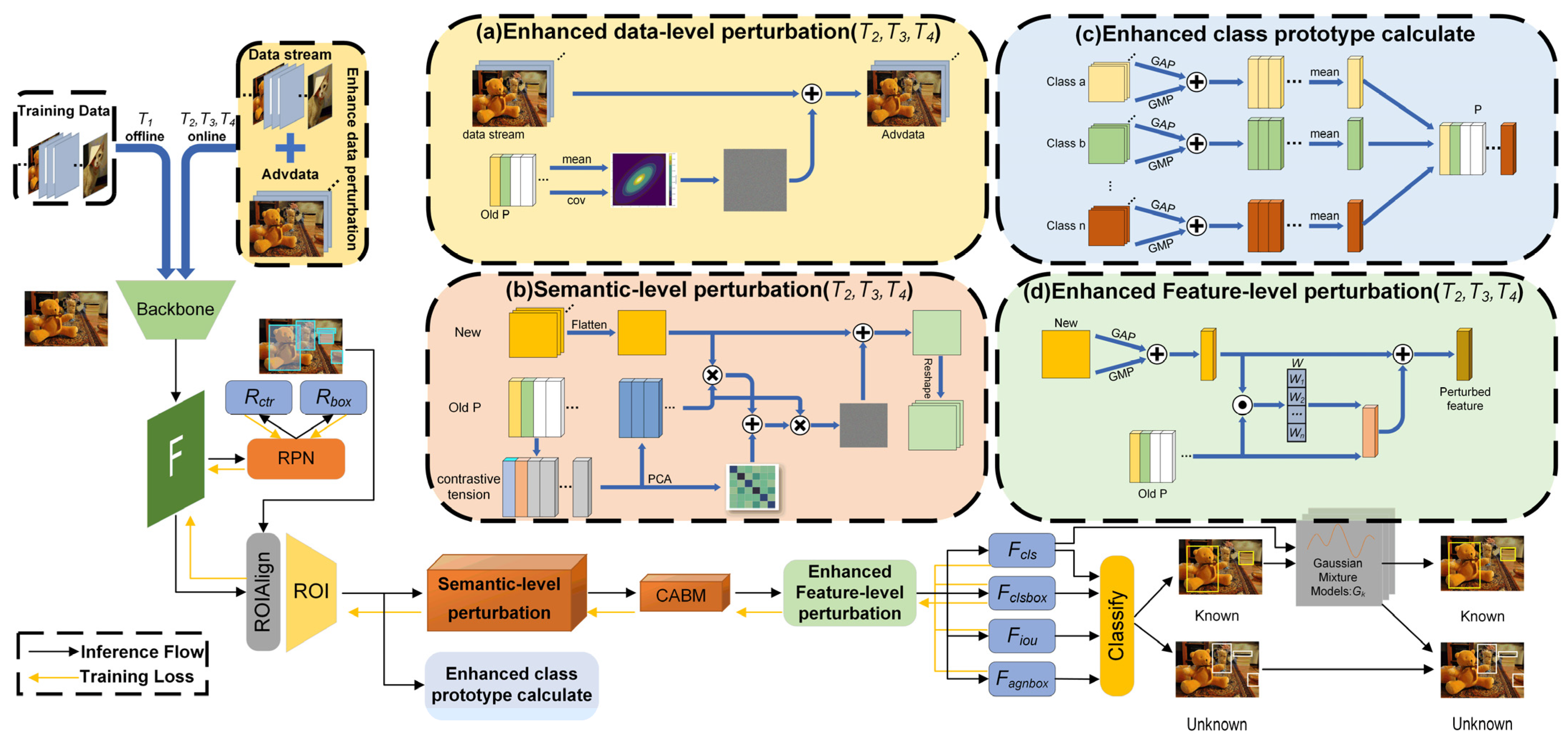
3.2. Overall Architecture
3.3. Enhanced Category Prototype Computation
3.3.1. Inter-Class Prototype Computation via Pooling and Mean
| Algorithm 1 Enhanced Category Prototype Computation |
| Input: : Feature maps of all instances in current class c, shape [N, C, H, W] : Number of most representative samples to retain (e.g., 50) : Weight coefficient for GAP and GMP fusion (default 0.5) Output: : Final prototype vector for class c 1: Initialize empty list candidate_features = [] 2: For i in range(N): 3: feature map [i] 4: Compute GAP and GMP: 5: gap GlobalAveragePooling(feature_map) 6: gmp GlobalMaxPooling(feature_map) 7: Fuse to form candidate feature: 8: fused_feature × gap + (1 − ) × gmp 9: candidate_features.append(fused_feature) 10: end 11: center Mean(candidate_features) 12: distance_list [] 13: For feat in candidate_features: 14: dist = EuclideanDistance(feat, center) 15: distance_list.append((feat, dist)) 16: end 17: distance_list sort(keylambda x: x [1]) 18: Retain closest features: 19: selected_feats [feat for feat, _ in distance_list[:]] 20: Mean(selected_feats) 21: Normalize() 22: Return |
3.3.2. Prototype Distance-Based Sample Selection Strategy
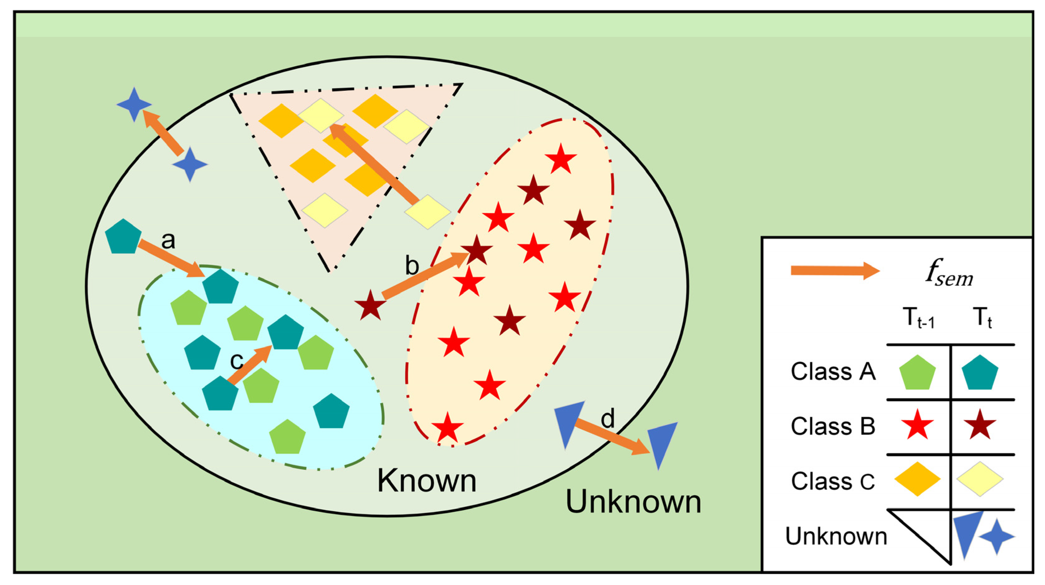
3.4. Semantic-Level Perturbation via Prototype-Contrastive Tension
| Algorithm 2 Semantic-Level Perturbation | |
| Input: : Feature map from ROI Pooling : Prototype matrix from previous tasks () : Blending hyperparameter (e.g., 0.4) Output: : Perturbed features after semantic-level perturbation 1: Flatten(f) 2: 3: For i in range(): 4: For j in range(N): 5: if : 6: .append()// 7: end 8: end 9: ←Matrixization () # 10: pca_model ← PCA() 11: pca_model.fit() 12: cumulative_variance ← CumulativeSum(pca_model.explained_variance_ratio_) 13: D ← FirstIndexWhere(cumulative_variance ≥ 0.9) + 1 14: ← TopDPrincipalComponents(pca_model) 15: ← 16: ← Covariance() 17: ← Cholesky() 18: ← SampleFromStandardGaussian() 19: ← 20: ← 21: ← Reshape(f_gen_sem) 22: ← 23: Return |
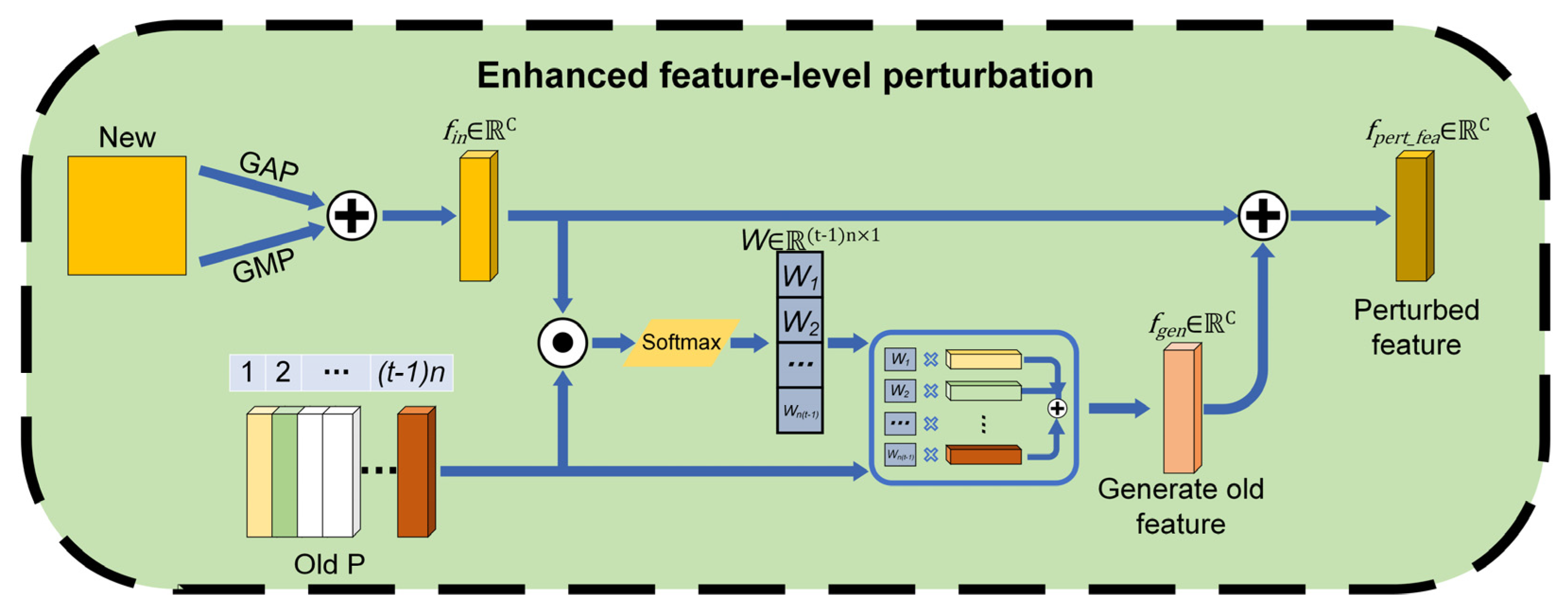
3.5. Enhanced Feature-Level Perturbations via Similarity Calculation
| Algorithm 3 Feature-Level Perturbation | ||
| Input: : Feature map from CABM : Prototype memory matrix : Blending coefficient (e.g., 0.6) Output: : Perturbed feature map 1: Compute GAP and GMP of feature f: 2: ← GMP(f) 3: ← GMP(f) 4: Fuse into input feature vector: 5: ← 0.5 × ( + ) 6: Compute cosine similarity between and each prototype in M: 7: For each prototype ∈ M: 8: ← 9: Compute attention weights via Softmax: 10: W ← Softmax() 11: Generate perturbation feature from weighted sum: 12: ← 13: Fuse with original feature to obtain final perturbation: 14: ← 15: Return |
3.6. Enhanced Data-Level Perturbations via Multivariate Gaussian Distribution
| Algorithm 4 Enhanced Data-Level Perturbations | |
| Input: : Boundary features for previous : Training data for current task : Perturbation ratio (e.g., 0.05) Output: : Augmented training data 1: For each class c in : 2: Compute class mean vector ← 3: Compute class covariance matrix ← 4: end 5: Compute global mean vector ← 6: Compute global covariance matrix ← 7: Define multivariate Gaussian distribution 8: Sample from with shape matching 9: Randomly select ⌊ × ||⌋ samples from to form subset 10: For each x ∈: 11: Generate adversarial sample: ← x + 12: Add x with in 13: end 14: Return |
4. Experience
4.1. Experiment Settings
4.1.1. Datasets
4.1.2. Baseline and Metrics
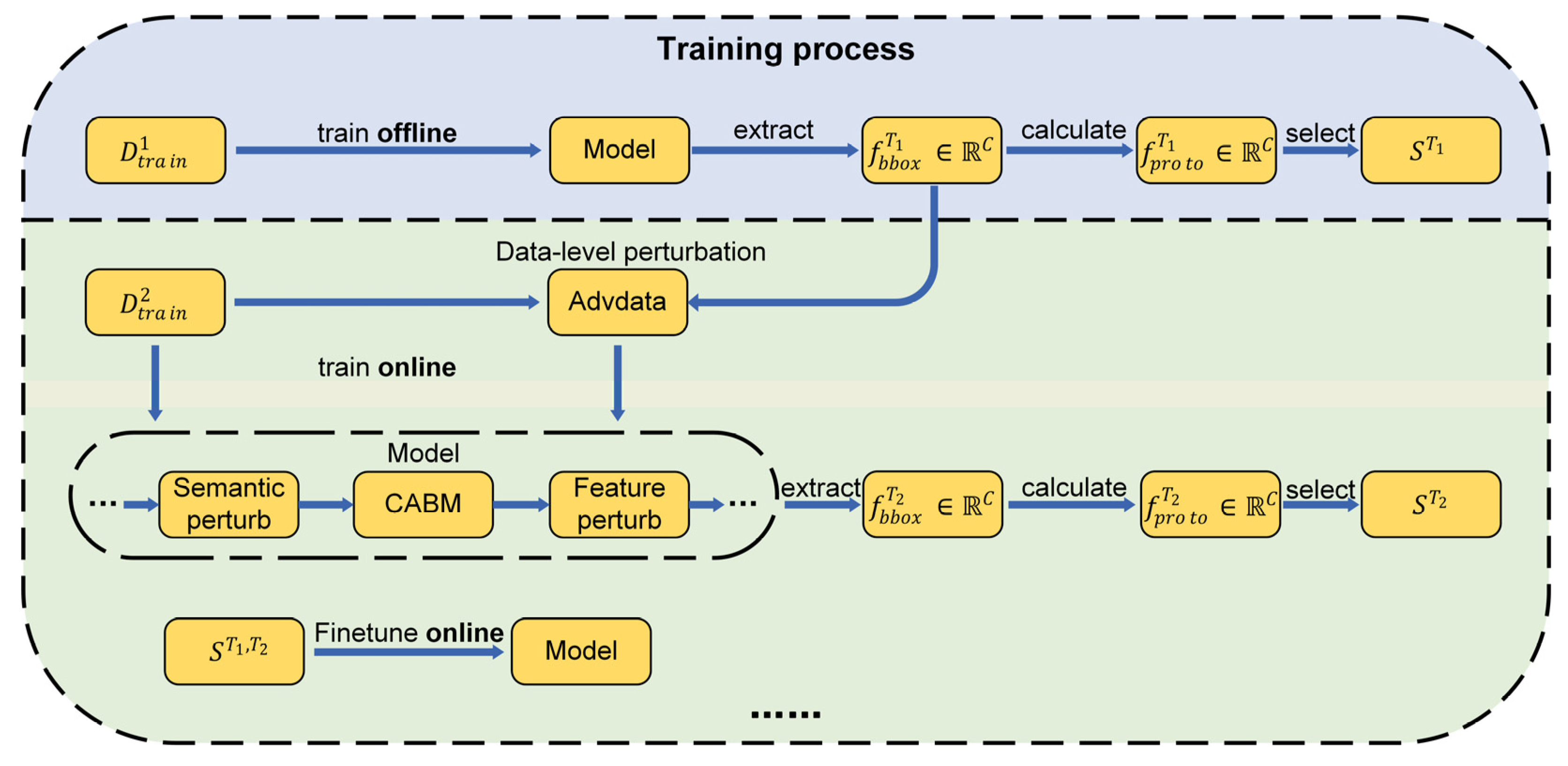
4.1.3. Training Process
4.1.4. Implementation Details
4.2. Results and Analysis
4.3. Incremental Object Detection
4.4. Ablation Study
4.4.1. Ablation Study of the PSMP Module
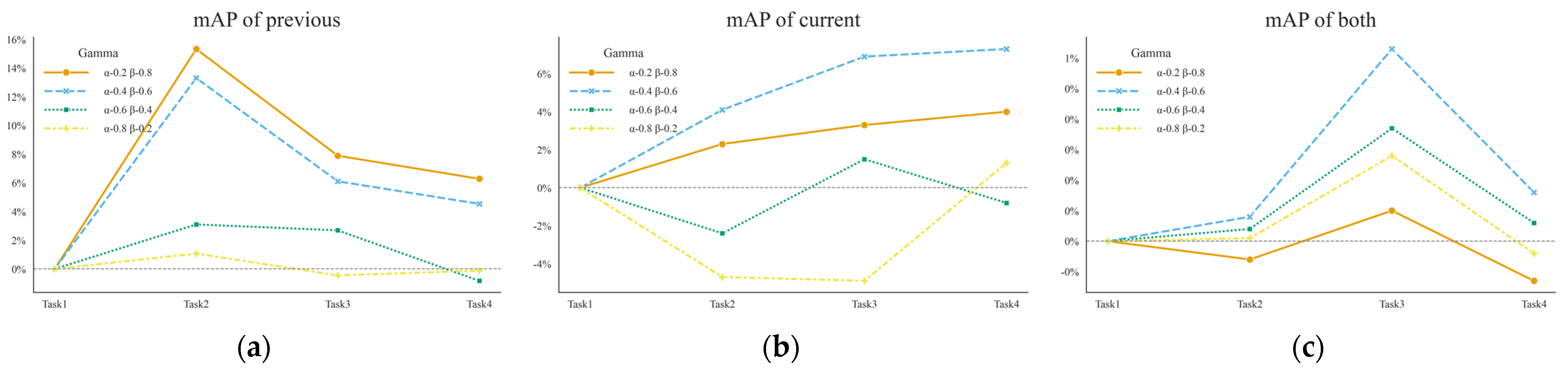
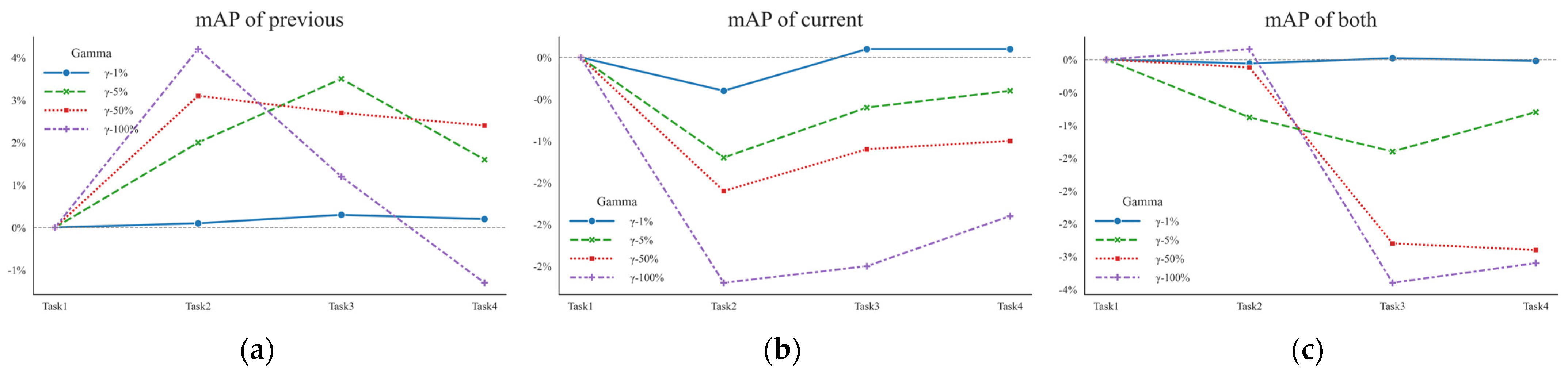
4.4.2. Ablation Study of Perturbation Intensity
4.4.3. Ablation Study of PSMP’s Performance
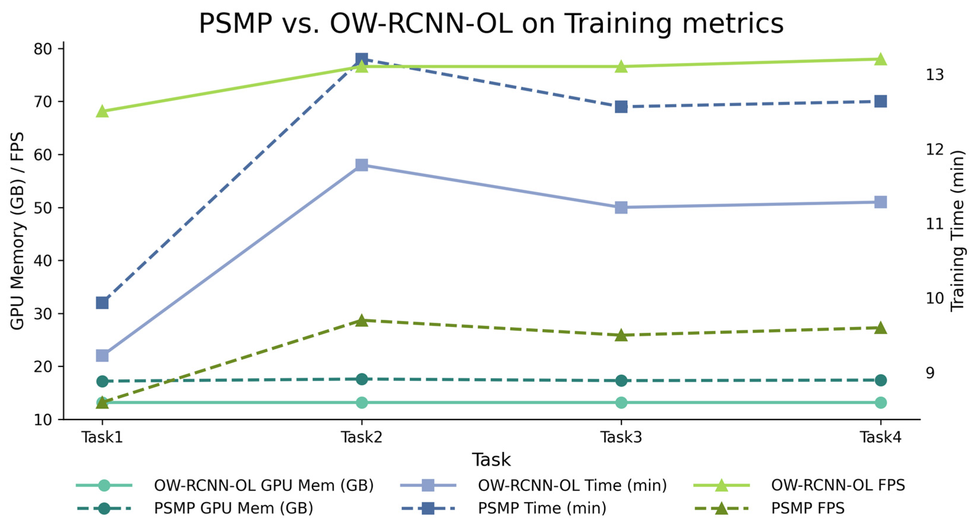
- The prototype computation module introduces minimal overhead, with only ~1 GB increase in memory and 4 additional minutes per training stage.
- Semantic-level and data-level perturbations consume similar amounts of memory, and each add approximately 7 min to the training time. However, semantic perturbation leads to the most noticeable drop in training FPS.
- Feature-level perturbation incurs the least memory overhead and increases training time by only 2 min, with a slight decrease in FPS.
- As no perturbations are applied during inference, PSMP and OW-RCNN-OL exhibit identical inference-time performance metrics, which are therefore omitted here.

| PSMP(OW-RCNN) | GPU Memory | Per-Stage Time | Training FPS |
|---|---|---|---|
| +1.0 GB | +4 min | 12.0 | |
| +0.7 GB | +4 min | 11.2 | |
| +1.4 GB | +7 min | 11.6 | |
| +1.3 GB | +7 min | 10.8 | |
| Total | +4.2 GB | +20 min | 10.6 |
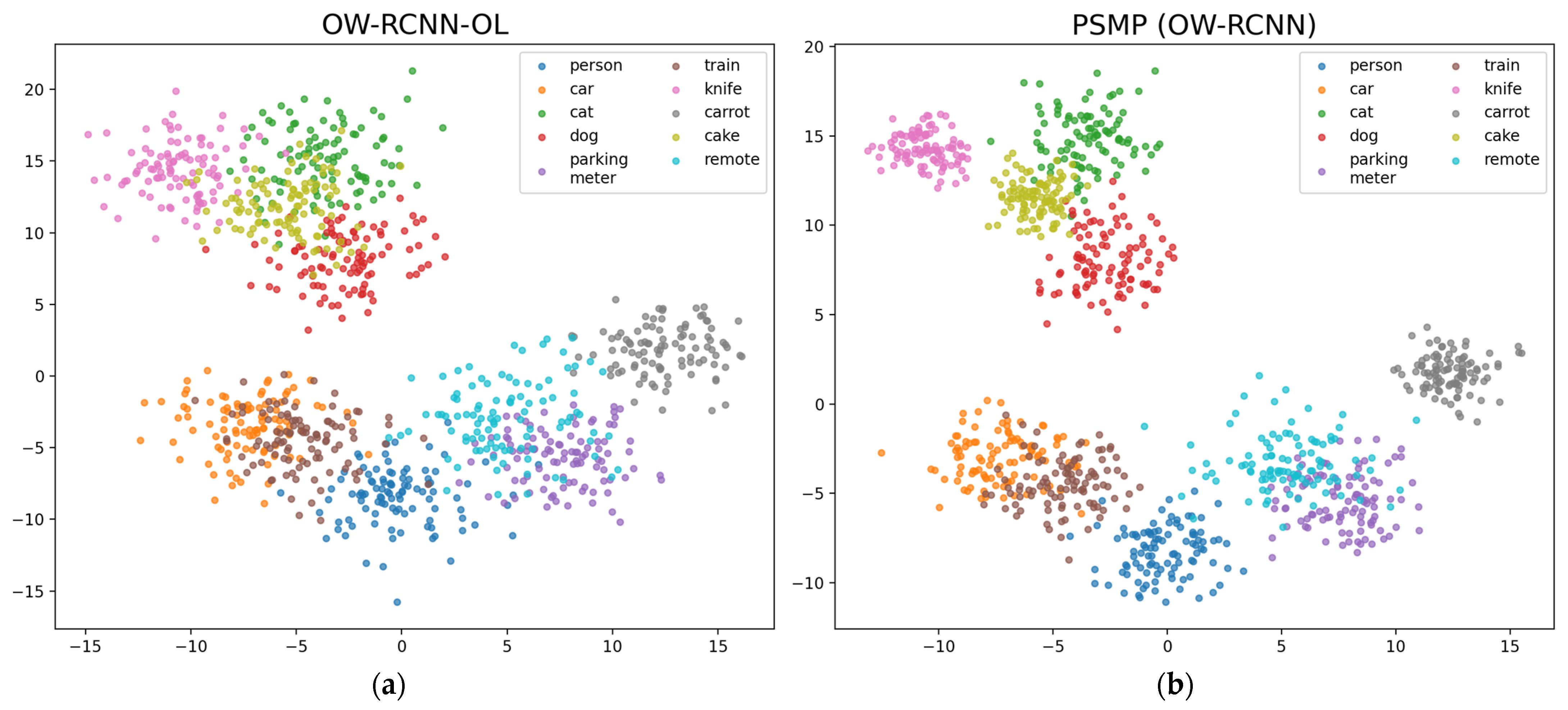
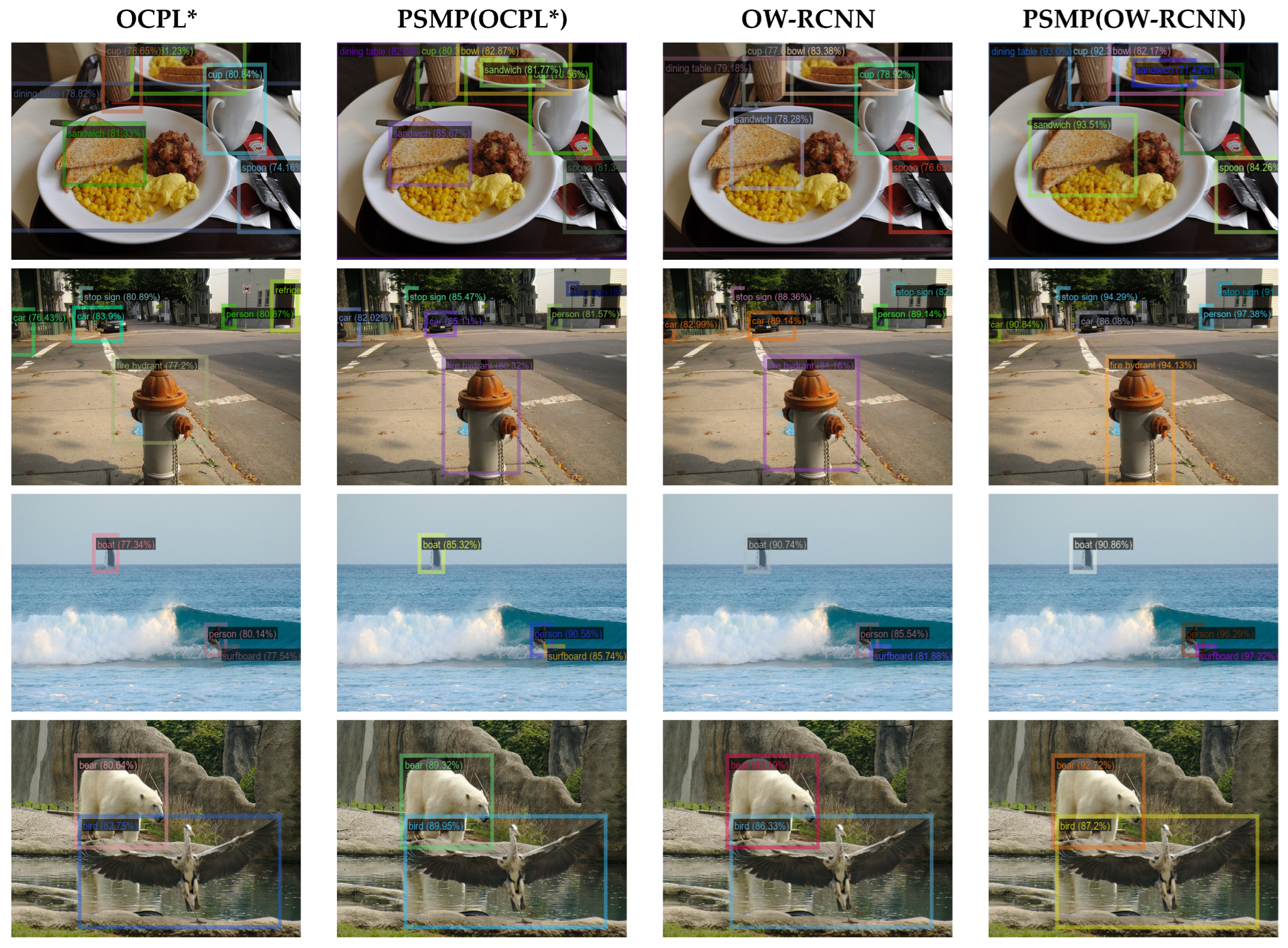
4.5. Visualization
5. Discussion
6. Conclusions
Author Contributions
Funding
Data Availability Statement
Acknowledgments
Conflicts of Interest
References
- He, K.; Gkioxari, G.; Dollár, P.; Girshick, R. Mask r-cnn. In Proceedings of the IEEE International Conference on Computer Vision, Venice, Italy, 22–29 October 2017; pp. 2961–2969. [Google Scholar]
- Lin, T.-Y.; Goyal, P.; Girshick, R.; He, K.; Dollár, P. Focal loss for dense object detection. In Proceedings of the IEEE International Conference on Computer Vision, Venice, Italy, 22–29 October 2017; pp. 2980–2988. [Google Scholar]
- Lin, T.-Y.; Maire, M.; Belongie, S.; Hays, J.; Perona, P.; Ramanan, D.; Dollár, P.; Zitnick, C.L. Microsoft coco: Common objects in context. In Proceedings of the Computer Vision–ECCV 2014: 13th European Conference, Zurich, Switzerland, 6–12 September 2014; Proceedings, Part V 13. pp. 740–755. [Google Scholar]
- Ren, S.; He, K.; Girshick, R.; Sun, J. Faster r-cnn: Towards real-time object detection with region proposal networks. Adv. Neural Inf. Process. Syst. 2015, 28. [Google Scholar] [CrossRef] [PubMed]
- Girshick, R. Fast r-cnn. In Proceedings of the IEEE International Conference on Computer Vision, Santiago, Chile, 7–13 December 2015; pp. 1440–1448. [Google Scholar]
- Redmon, J.; Divvala, S.; Girshick, R.; Farhadi, A. You only look once: Unified, real-time object detection. In Proceedings of the IEEE Conference on Computer Vision and Pattern Recognition, Las Vegas, NV, USA, 27–30 June 2016; pp. 779–788. [Google Scholar]
- Redmon, J.; Farhadi, A. YOLO9000: Better, faster, stronger. In Proceedings of the IEEE Conference on Computer Vision and Pattern Recognition, Honolulu, HI, USA, 21–26 July 2017; pp. 7263–7271. [Google Scholar]
- Wang, C.-Y.; Bochkovskiy, A.; Liao, H.-Y.M. YOLOv7: Trainable bag-of-freebies sets new state-of-the-art for real-time object detectors. In Proceedings of the IEEE/CVF Conference on Computer Vision and Pattern Recognition, Vancouver, BC, Canada, 17–24 June 2023; pp. 7464–7475. [Google Scholar]
- Vaswani, A.; Shazeer, N.; Parmar, N.; Uszkoreit, J.; Jones, L.; Gomez, A.N.; Kaiser, L.; Polosukhin, I. Attention is all you need. Adv. Neural Inf. Process. Syst. 2017, 30, 2. [Google Scholar]
- Zhu, X.; Su, W.; Lu, L.; Li, B.; Wang, X.; Dai, J. Deformable detr: Deformable transformers for end-to-end object detection. arXiv 2020, arXiv:2010.04159. [Google Scholar]
- Joseph, K.; Khan, S.; Khan, F.S.; Balasubramanian, V.N. Towards open world object detection. In Proceedings of the IEEE/CVF Conference on Computer Vision and Pattern Recognition, Nashville, TN, USA, 20–25 June 2021; pp. 5830–5840. [Google Scholar]
- Gupta, A.; Narayan, S.; Joseph, K.; Khan, S.; Khan, F.S.; Shah, M. Ow-detr: Open-world detection transformer. In Proceedings of the IEEE/CVF Conference on Computer Vision and Pattern Recognition, Long Beach, CA, USA, 20 June 2019; pp. 9235–9244. [Google Scholar]
- Zhao, X.; Liu, X.; Shen, Y.; Qiao, Y.; Ma, Y.; Wang, D. Revisiting Open World Object Detection. IEEE Trans. Circuits Syst. Video Technol. 2023, 34, 3496–3509. [Google Scholar] [CrossRef]
- Zohar, O.; Wang, K.-C.; Yeung, S. PROB: Probabilistic Objectness for Open World Object Detection. In Proceedings of the IEEE/CVF Conference on Computer Vision and Pattern Recognition (CVPR), Vancouver, BC, Canada, 24 June 2023; pp. 11444–11453. [Google Scholar]
- Ma, S.; Wang, Y.; Wei, Y.; Fan, J.; Li, T.H.; Liu, H.; Lv, F. CAT: LoCalization and IdentificAtion Cascade Detection Transformer for Open-World Object Detection. In Proceedings of the IEEE/CVF Conference on Computer Vision and Pattern Recognition (CVPR), Vancouver, BC, Canada, 24 June 2023; pp. 19681–19690. [Google Scholar]
- Yu, J.; Ma, L.; Li, Z.; Peng, Y.; Xie, S. Open-world object detection via discriminative class prototype learning. In Proceedings of the 2022 IEEE International Conference on Image Processing (ICIP), Bordeaux, France, 16–19 October 2022. [Google Scholar]
- Pershouse, D.; Dayoub, F.; Miller, D.; Sünderhauf, N. Addressing the challenges of open-world object detection. arXiv 2023, arXiv:2303.14930. [Google Scholar] [CrossRef]
- Chen, Y.; Ma, L.; Jing, L.; Yu, J. BSDP: Brain-inspired Streaming Dual-level Perturbations for Online Open World Object Detection. Pattern Recognit. 2024, 152, 110472. [Google Scholar] [CrossRef]
- Van der Groen, O.; Potok, W.; Wenderoth, N.; Edwards, G.; Mattingley, J.B.; Edwards, D. Using noise for the better: The effects of transcranial random noise stimulation on the brain and behavior. Neurosci. Biobehav. Rev. 2022, 138, 104702. [Google Scholar] [CrossRef] [PubMed]
- Girshick, R.; Donahue, J.; Darrell, T.; Malik, J. Region-based convolutional networks for accurate object detection and segmentation. IEEE Trans. Pattern Anal. Mach. Intell. 2015, 38, 142–158. [Google Scholar] [CrossRef] [PubMed]
- Cai, Z.; Vasconcelos, N. Cascade r-cnn: Delving into high quality object detection. In Proceedings of the IEEE Conference on Computer Vision and Pattern Recognition, Salt Lake City, UT, USA, 18–23 June 2018; pp. 6154–6162. [Google Scholar]
- Sun, P.; Zhang, R.; Jiang, Y.; Kong, T.; Xu, C.; Zhan, W.; Tomizuka, M.; Li, L.; Yuan, Z.; Wang, C. Sparse r-cnn: End-to-end object detection with learnable proposals. In Proceedings of the IEEE/CVF Conference on Computer Vision and Pattern Recognition, New Orleans, LA, USA, 18–24 June 2022; pp. 14454–14463. [Google Scholar]
- Liu, W.; Anguelov, D.; Erhan, D.; Szegedy, C.; Reed, S.; Fu, C.-Y.; Berg, A.C. SSD: Single Shot MultiBox Detector. In Proceedings of the 14th European Conference on Computer Vision (ECCV), Amsterdam, The Netherlands, 11–14 October 2016; pp. 21–37. [Google Scholar]
- Khan, S.; Naseer, M.; Hayat, M.; Zamir, S.W.; Khan, F.S.; Shah, M. Transformers in vision: A survey. ACM Comput. Surv. (CSUR) 2022, 54, 1–41. [Google Scholar] [CrossRef]
- Dosovitskiy, A.; Beyer, L.; Kolesnikov, A.; Weissenborn, D.; Zhai, X.; Unterthiner, T.; Dehghani, M.; Minderer, M.; Heigold, G.; Gelly, S.; et al. An Image is Worth 16x16 Words: Transformers for Image Recognition at Scale. arXiv 2021, arXiv:2010.11929. [Google Scholar] [CrossRef]
- Ranftl, R.; Bochkovskiy, A.; Koltun, V. Vision transformers for dense prediction. In Proceedings of the IEEE/CVF International Conference on Computer Vision, Montreal, QC, Canada, 10–17 October 2021; pp. 12179–12188. [Google Scholar]
- Fan, H.; Xiong, B.; Mangalam, K.; Li, Y.; Yan, Z.; Malik, J.; Feichtenhofer, C. Multiscale vision transformers. In Proceedings of the IEEE/CVF International Conference on Computer Vision, Montreal, BC, Canada, 10–17 October 2021; pp. 6824–6835. [Google Scholar]
- Wang, W.; Xie, E.; Li, X.; Fan, D.-P.; Song, K.; Liang, D.; Lu, T.; Luo, P.; Shao, L. Pyramid vision transformer: A versatile backbone for dense prediction without convolutions. In Proceedings of the IEEE/CVF International Conference on Computer Vision, Montreal, QC, Canada, 10–17 October 2021; pp. 568–578. [Google Scholar]
- Carion, N.; Massa, F.; Synnaeve, G.; Usunier, N.; Kirillov, A.; Zagoruyko, S. End-to-End Object Detection with Transformers. arXiv 2020, arXiv:2005.12872. [Google Scholar]
- Wu, Z.; Lu, Y.; Chen, X.; Wu, Z.; Kang, L.; Yu, J. UC-OWOD: Unknown-Classified Open World Object Detection; Springer Nature: Cham, Switzerland; pp. 193–210.
- Shaheen, K.; Hanif, M.A.; Hasan, O.; Shafique, M. A Framework for Open World Object Detection. Artif. Intell. Evol. 2023, 4, 154–164. [Google Scholar] [CrossRef]
- Li, Y.; Wang, Y.; Wang, W.; Lin, D.; Li, B.; Yap, K. Open World Object Detection: A Survey. IEEE Trans. Circuits Syst. Video Technol. 2025, 35, 988–1008. [Google Scholar] [CrossRef]
- Mullappilly, S.S.; Gehlot, A.S.; Anwer, R.M.; Khan, F.S.; Cholakkal, H. Semi-supervised Open-World Object Detection. In Proceedings of the 38th AAAI Conference on Artificial Intelligence (AAAI)/36th Conference on Innovative Applications of Artificial Intelligence/14th Symposium on Educational Advances in Artificial Intelligence, Vancouver, BC, Canada, 20–27 February 2024; pp. 4305–4314. [Google Scholar]
- Ma, Z.; Zheng, Z.; Wei, J.; Yang, Y.; Shen, H.T. Instance-Dictionary Learning for Open-World Object Detection in Autonomous Driving Scenarios. IEEE Trans. Circuits Syst. Video Technol. 2024, 34, 3395–3408. [Google Scholar] [CrossRef]
- He, Y.; Chen, W.; Wang, S.; Liu, T.; Wang, M. Recalling Unknowns Without Losing Precision: An Effective Solution to Large Model-Guided Open World Object Detection. IEEE Trans. Image Process. 2025, 34, 729–742. [Google Scholar] [CrossRef] [PubMed]
- Xue, W.; Xu, G.; Yang, N.; Liu, J. Enhancing open-world object detection with AIGC-generated datasets and elastic weight consolidation. J. Supercomput. 2025, 81, 417. [Google Scholar] [CrossRef]
- Fang, R.; Pang, G.; Miao, W.; Bai, X.; Zheng, J.; Ning, X. Unsupervised Recognition of Unknown Objects for Open-World Object Detection. IEEE Trans. Neural Netw. Learn. Syst. 2025, 36, 11340–11354. [Google Scholar] [CrossRef] [PubMed]
- Zhao, R.; Wang, J.; Chen, Y.; Zheng, Z.; Cui, K.; Su, J. Class-Agnostic Detection of Unknown Objects from Foreground Improves Robust Open World Object Detection. In Proceedings of the 7th Chinese Conference on Pattern Recognition and Computer Vision, Urumqi, China, 18–20 October 2024; pp. 78–92. [Google Scholar]
- Jamonnak, S.; Guo, J.; He, W.; Gou, L.; Ren, L. OW-Adapter: Human-Assisted Open-World Object Detection with a Few Examples. IEEE Trans. Vis. Comput. Graph. 2024, 30, 694–704. [Google Scholar] [CrossRef] [PubMed]
- Kirkpatrick, J.; Pascanu, R.; Rabinowitz, N.; Veness, J.; Desjardins, G.; Rusu, A.A.; Milan, K.; Quan, J.; Ramalho, T.; Hassabis, D.; et al. Overcoming catastrophic forgetting in neural networks. Proc. Natl. Acad. Sci. USA 2017, 114, 3521–3526. [Google Scholar] [CrossRef] [PubMed]
- Li, Z.; Hoiem, D. Learning without forgetting. IEEE Trans. Pattern Anal. Mach. Intell. 2017, 40, 2935–2947. [Google Scholar] [CrossRef] [PubMed]
- Castro, F.M.; Marín-Jiménez, M.J.; Guil, N.; Schmid, C.; Alahari, K. End-to-end incremental learning. In Proceedings of the European Conference on Computer Vision (ECCV), Munich, Germany, 8–14 September 2018; pp. 233–248. [Google Scholar]
- Dong, N.; Zhang, Y.; Ding, M.; Bai, Y. Class-incremental object detection. Pattern Recognit. 2023, 139, 109488. [Google Scholar] [CrossRef]
- Sun, W.; Li, Q.; Zhang, J.; Wang, D.; Wang, W.; Geng, Y. Exemplar-free class incremental learning via discriminative and comparable parallel one-class classifiers. Pattern Recognit. 2023, 140, 109561. [Google Scholar] [CrossRef]
- Sun, Q.; Lyu, F.; Shang, F.; Feng, W.; Wan, L. Exploring example influence in continual learning. Adv. Neural Inf. Process. Syst. 2022, 35, 27075–27086. [Google Scholar]
- Tiwari, R.; Killamsetty, K.; Iyer, R.; Shenoy, P. Gcr: Gradient coreset based replay buffer selection for continual learning. In Proceedings of the IEEE/CVF Conference on Computer Vision and Pattern Recognition, New Orleans, LA, USA, 19–20 June 2022; pp. 99–108. [Google Scholar]
- Riemer, M.; Cases, I.; Ajemian, R.; Liu, M.; Rish, I.; Tu, Y.; Tesauro, G. Learning to learn without forgetting by maximizing transfer and minimizing interference. arXiv 2018, arXiv:1810.11910. [Google Scholar]
- Zhuang, C.; Huang, S.; Cheng, G.; Ning, J. Multi-criteria selection of rehearsal samples for continual learning. Pattern Recognit. 2022, 132, 108907. [Google Scholar] [CrossRef]
- Rebuffi, S.-A.; Kolesnikov, A.; Sperl, G.; Lampert, C.H. icarl: Incremental classifier and representation learning. In Proceedings of the IEEE conference on Computer Vision and Pattern Recognition, Las Vegas, NV, USA, 27–30 June 2016; pp. 2001–2010. [Google Scholar]
- Dong, J.; Liang, W.; Cong, Y.; Sun, G. Heterogeneous forgetting compensation for class-incremental learning. In Proceedings of the IEEE/CVF International Conference on Computer Vision, Seattle, WA, USA, 16–22 June 2024; pp. 11742–11751. [Google Scholar]
- Yang, D.; Zhou, Y.; Zhang, A.; Sun, X.; Wu, D.; Wang, W.; Ye, Q. Multi-View correlation distillation for incremental object detection. Pattern Recognit. 2022, 131, 108863. [Google Scholar] [CrossRef]
- Wang, J.; Wang, X.; Shang-Guan, Y.; Gupta, A. Wanderlust: Online Continual Object Detection in the Real World. In Proceedings of the 2021 IEEE/CVF International Conference on Computer Vision (ICCV), Montreal, QC, Canada, 10–17 October 2021; pp. 10809–10818. [Google Scholar]
- Li, M.; Yan, Z.; Li, C. Class Incremental Learning with Important and Diverse Memory; Springer Nature: Cham, Switzerland; pp. 164–175.
- Nokhwal, S.; Kumar, N. DSS: A Diverse Sample Selection Method to Preserve Knowledge in Class-Incremental Learning. In Proceedings of the 2023 10th International Conference on Soft Computing & Machine Intelligence (ISCMI), Mexico City, Mexico, 25–26 November 2023; pp. 178–182. [Google Scholar]
- Zeng, L.; Chen, X.; Shi, X.; Shen, H.T. Feature Noise Boosts DNN Generalization Under Label Noise. IEEE Trans. Neural Netw. Learn. Syst. 2025, 36, 7711–7724. [Google Scholar] [CrossRef] [PubMed]
- Dhifallah, O.; Lu, Y. On the inherent regularization effects of noise injection during training. In Proceedings of the International Conference on Machine Learning, PMLR, Virtual, 18–24 July 2021; pp. 2665–2675. [Google Scholar]
- Yuan, X.; Li, J.; Kuruoglu, E.E. Robustness enhancement in neural networks with alpha-stable training noise. Digit. Signal Process. 2025, 156, 104778. [Google Scholar] [CrossRef]
- Kim, H.-E.; Hwang, S.; Cho, K. Semantic Noise Modeling for Better Representation Learning. arXiv 2016, arXiv:1611.01268. [Google Scholar] [CrossRef]
- Woo, S.; Park, J.; Lee, J.-Y.; Kweon, I.S. Cbam: Convolutional block attention module. In Proceedings of the European Conference on Computer Vision (ECCV), Munich, Germany, 8–14 September 2018; pp. 3–19. [Google Scholar]
- Everingham, M.; Van Gool, L.; Williams, C.K.I.; Winn, J.; Zisserman, A. The Pascal Visual Object Classes (VOC) Challenge. Int. J. Comput. Vis. 2010, 88, 303–338. [Google Scholar] [CrossRef]
- Bansal, A.; Sikka, K.; Sharma, G.; Chellappa, R.; Divakaran, A. Zero-Shot Object Detection. In Computer Vision—ECCV 2018; Springer Nature: Cham, Switzerland, 2018; pp. 397–414. [Google Scholar]
- Dhamija, A.R.; Günther, M.; Ventura, J.; Boult, T.E. The Overlooked Elephant of Object Detection: Open Set. In Proceedings of the 2020 IEEE Winter Conference on Applications of Computer Vision (WACV), Snowmass Village, CO, USA, 1–5 March 2020; pp. 1010–1019. [Google Scholar]
- Miller, D.; Zhou, Z.; Bambos, N.; Ben-Gal, I. Optimal Sensing for Patient Health Monitoring. In Proceedings of the 2018 IEEE International Conference on Communications (ICC), Kansas City, MO, USA, 20–24 May 2018; pp. 1–7. [Google Scholar]
- Wang, Y.; Yue, Z.; Hua, X.-S.; Zhang, H. Random boxes are open-world object detectors. In Proceedings of the IEEE/CVF International Conference on Computer Vision, Paris, France, 1–6 October 2023; pp. 6233–6243. [Google Scholar]
- Joseph, K.J.; Rajasegaran, J.; Khan, S.; Khan, F.S.; Balasubramanian, V.N. Incremental Object Detection via Meta-Learning. IEEE Trans. Pattern Anal. Mach. Intell. 2022, 44, 9209–9216. [Google Scholar] [CrossRef] [PubMed]
- Shmelkov, K.; Schmid, C.; Alahari, K. Incremental learning of object detectors without catastrophic forgetting. In Proceedings of the IEEE International Conference on Computer Vision, Venice, Italy, 22–29 October 2017; pp. 3400–3409. [Google Scholar]
- Peng, C.; Zhao, K.; Lovell, B.C. Faster ILOD: Incremental learning for object detectors based on faster RCNN. Pattern Recognit. Lett. 2020, 140, 109–115. [Google Scholar] [CrossRef]


| Task 1 (Base Task) | Task 2 | Task 3 | Task 4 | |
|---|---|---|---|---|
| Semantic split | VOC classes | Outdoor, accessories, appliance, truck | Sports, food | Electronic, indoor, kitchen, furniture |
| Training images | 16,551 | 45,520 | 39,402 | 40,260 |
| Exemplars | 1000 | 1000 | 1000 | 1000 |
| Test images | 10,246 | 10,246 | 10,246 | 10,246 |
| Task IDs | Task 1 | Task 2 | Task 3 | Task 4 | |||||||||
|---|---|---|---|---|---|---|---|---|---|---|---|---|---|
| mAP (↑) | UR | mAP (↑) | UR | mAP (↑) | UR | mAP (↑) | |||||||
| C | (↑) | P | C | Both | (↑) | P | C | Both | (↑) | P | C | Both | |
| ORE* | 56.21 | 5.24 | 52.84 | 28.73 | 40.79 | 2.95 | 38.20 | 13.05 | 30.07 | 3.93 | 29.64 | 14.21 | 25.52 |
| OCPL* | 56.32 | 8.23 | 51.93 | 28.86 | 40.40 | 7.51 | 39.25 | 14.79 | 31.44 | 12.28 | 31.47 | 14.80 | 26.24 |
| OW-RCNN [17] | 62.41 | 37.52 | 48.20 | 41.58 | 45.14 | 39.67 | 44.31 | 30.94 | 40.08 | 42.18 | 39.82 | 28.07 | 36.94 |
| UC-OWOD* | 56.38 | 32.44 | 48.83 | 45.75 | 46.04 | 35.41 | 30.14 | 26.82 | 27.43 | 37.49 | 28.24 | 25.79 | 26.11 |
| RandBox | 60.4 | 10.5 | 47.26 | 43.88 | 45.07 | 6.25 | 42.17 | 38.34 | 39.28 | 7.67 | 36.02 | 33.94 | 34.81 |
| ORE*-OL | 56.21 | 5.24 | 51.44 | 22.84 | 37.22 | 3.42 | 37.28 | 12.59 | 28.73 | 2.45 | 28.47 | 13.88 | 23.12 |
| OCPL*-OL | 56.32 | 8.23 | 52.20 | 25.37 | 38.35 | 7.91 | 39.11 | 13.66 | 30.11 | 9.32 | 29.25 | 14.01 | 25.24 |
| OW-RCNN-OL | 62.41 | 37.52 | 46.98 | 40.32 | 44.43 | 40.28 | 42.81 | 29.19 | 39.26 | 40.71 | 38.76 | 27.40 | 36.07 |
| UC-OWOD*-OL | 56.38 | 32.44 | 49.46 | 42.90 | 44.28 | 35.88 | 29.97 | 25.06 | 26.32 | 34.85 | 26.11 | 25.37 | 25.39 |
| RandBox-OL | 60.4 | 10.5 | 48.04 | 40.39 | 43.97 | 5.98 | 41.32 | 36.33 | 38.50 | 6.94 | 34.53 | 31.71 | 32.55 |
| PSMP(ORE*) | 56.21 | 5.24 | 52.98 | 23.47 | 38.49 | 3.51 | 38.92 | 12.33 | 30.82 | 3.21 | 30.26 | 14.08 | 25.20 |
| PSMP(OCPL*) | 56.32 | 8.23 | 53.27 | 26.83 | 39.55 | 7.68 | 40.70 | 14.25 | 31.29 | 11.83 | 32.52 | 14.67 | 26.51 |
| PSMP(UC-OWOD*) | 56.38 | 32.44 | 50.66 | 44.34 | 45.77 | 35.69 | 30.84 | 26.55 | 28.01 | 35.08 | 28.29 | 26.15 | 27.04 |
| PSMP(RandBox) | 60.4 | 10.5 | 49.33 | 42.34 | 45.28 | 6.44 | 42.86 | 36.54 | 39.66 | 8.01 | 36.70 | 33.18 | 35.22 |
| BSDP(OW-RCNN) | 62.41 | 37.52 | 52.45 | 40.27 | 44.58 | 40.31 | 44.57 | 29.10 | 41.22 | 44.29 | 40.08 | 26.01 | 36.44 |
| PSMP(OW-RCNN) | 62.41 | 37.52 | 54.58 | 41.29 | 45.02 | 42.14 | 46.22 | 30.88 | 42.50 | 45.28 | 41.27 | 27.91 | 37.68 |
| Task IDs | Task 1 | Task 2 | Task 3 | |||
|---|---|---|---|---|---|---|
| WI | A-OSE | WI | A-OSE | WI | A-OSE | |
| (↓) | (↓) | (↓) | (↓) | (↓) | (↓) | |
| ORE* | 0.0580 | 11428 | 0.0295 | 10631 | 0.0214 | 9471 |
| OCPL* | 0.0462 | 5615 | 0.0228 | 5944 | 0.0165 | 4852 |
| OW-RCNN [17] | 0.0537 | 6882 | 0.0248 | 4722 | 0.0172 | 3827 |
| ORE*-OL | 0.0580 | 11428 | 0.0384 | 11377 | 0.0192 | 8925 |
| OCPL*-OL | 0.0462 | 5615 | 0.0242 | 5865 | 0.0174 | 4221 |
| OW-RCNN-OL | 0.0537 | 6882 | 0.0261 | 4006 | 0.0168 | 3428 |
| PSMP(ORE*) | 0.0580 | 11428 | 0.0297 | 12875 | 0.0260 | 7931 |
| PSMP(OCPL*) | 0.0462 | 5615 | 0.0249 | 5437 | 0.0179 | 4394 |
| BSDP(OW-RCNN) | 0.0537 | 6882 | 0.0226 | 3922 | 0.0174 | 4155 |
| PSMP(OW-RCNN) | 0.0537 | 6882 | 0.0213 | 3719 | 0.0160 | 3107 |
| 10 + 10 Settings | Table | Dog | Horse | Bike | Person | Plant | Sheep | Sofa | Train | TV | mAP |
|---|---|---|---|---|---|---|---|---|---|---|---|
| ILOD [66] | 59.7 | 72.7 | 73.5 | 73.2 | 66.3 | 29.5 | 63.4 | 61.6 | 69.3 | 62.2 | 63.1 |
| Faster ILOD [67] | 36.7 | 70.9 | 66.8 | 67.6 | 66.1 | 24.7 | 63.1 | 48.1 | 57.1 | 43.6 | 62.2 |
| iOD [65] | 60.1 | 66.4 | 76.0 | 72.6 | 74.6 | 39.7 | 64.0 | 60.2 | 68.5 | 60.5 | 66.3 |
| ORE [11] | 56.1 | 70.4 | 80.2 | 72.3 | 81.8 | 42.7 | 71.6 | 68.1 | 77.0 | 67.7 | 64.6 |
| OCPL* | 46.1 | 50.8 | 65.2 | 66.0 | 71.9 | 21.6 | 49.8 | 54.6 | 68.5 | 46.3 | 64.3 |
| OW-RCNN [17] | 58.8 | 42.9 | 63.5 | 58.2 | 67.6 | 28.9 | 36.3 | 66.8 | 77.5 | 59.6 | 65.1 |
| PSMP(ORE*) | 36.7 | 69.3 | 77.4 | 76.6 | 70.8 | 38.2 | 70.7 | 52.2 | 63.9 | 59.9 | 67.9 |
| PSMP(OCPL*) | 52.2 | 61.3 | 72.4 | 70.0 | 69.7 | 30.7 | 64.3 | 36.5 | 60.1 | 56.6 | 68.5 |
| PSMP(OW-RCNN) | 51.3 | 64.2 | 68.8 | 84.3 | 64.4 | 37.7 | 50.6 | 48.3 | 48.7 | 60.8 | 69.1 |
| 15 + 5 Settings | Table | Dog | Horse | Bike | Person | Plant | Sheep | Sofa | Train | TV | mAP |
| ILOD [66] | 59.0 | 75.8 | 71.8 | 78.6 | 69.6 | 33.7 | 61.5 | 63.1 | 71.7 | 62.2 | 65.9 |
| Faster ILOD [67] | 63.1 | 78.6 | 80.5 | 78.4 | 80.4 | 36.7 | 61.7 | 59.3 | 67.9 | 59.1 | 67.9 |
| iOD [65] | 61.8 | 74.7 | 81.6 | 77.5 | 80.2 | 37.8 | 58.0 | 54.6 | 73.0 | 56.1 | 67.8 |
| ORE [11] | 55.4 | 76.7 | 86.2 | 78.5 | 82.1 | 32.8 | 63.6 | 54.7 | 77.7 | 64.6 | 68.5 |
| OCPL* | 75.5 | 81.2 | 89.2 | 84.4 | 83.3 | 19.1 | 25.2 | 24.0 | 65.1 | 36.8 | 69.5 |
| OW-RCNN [17] | 79.3 | 83.7 | 82.6 | 80.7 | 81.8 | 54.2 | 39.1 | 43.7 | 31.5 | 47.3 | 72.8 |
| PSMP(ORE*) | 61.5 | 79.2 | 90.1 | 88.7 | 86.6 | 42.3 | 68.8 | 50.7 | 48.2 | 52.9 | 74.7 |
| PSMP(OCPL*) | 82.4 | 87.0 | 85.2 | 84.5 | 84.1 | 58.2 | 47.6 | 51.3 | 42.9 | 50.1 | 76.0 |
| PSMP(OW-RCNN) | 81.7 | 88.1 | 86.9 | 84.3 | 85.4 | 59.6 | 48.3 | 52.1 | 45.7 | 54.3 | 77.1 |
| 19 + 1 Settings | Table | Dog | Horse | Bike | Person | Plant | Sheep | Sofa | Train | TV | mAP |
| ILOD [66] | 64.8 | 77.2 | 80.8 | 77.5 | 70.1 | 42.3 | 67.5 | 64.4 | 76.7 | 62.7 | 68.3 |
| Faster ILOD [67] | 58.7 | 78.8 | 81.8 | 75.3 | 77.4 | 43.1 | 73.8 | 61.7 | 69.8 | 61.1 | 68.6 |
| iOD [65] | 63.2 | 78.5 | 82.7 | 79.1 | 79.9 | 44.1 | 73.2 | 66.3 | 76.4 | 57.6 | 70.2 |
| ORE [11] | 54.6 | 72.8 | 85.9 | 81.7 | 82.4 | 44.8 | 75.8 | 68.2 | 75.7 | 60.1 | 68.9 |
| OCPL* | 74.4 | 86.1 | 88.7 | 87.6 | 85.4 | 50.1 | 83.7 | 74.9 | 77.8 | 48.5 | 77.1 |
| OW-RCNN [17] | 76.9 | 82.3 | 79.5 | 77.6 | 78.8 | 74.1 | 75.6 | 78.3 | 80.1 | 58.3 | 78.0 |
| PSMP(ORE*) | 79.8 | 84.2 | 81.2 | 80.3 | 81.0 | 80.5 | 82.7 | 83.8 | 85.3 | 54.1 | 81.1 |
| PSMP(OCPL*) | 82.6 | 86.0 | 82.8 | 81.4 | 82.9 | 82.1 | 84.0 | 84.7 | 85.3 | 52.6 | 82.6 |
| PSMP(OW-RCNN) | 83.9 | 87.6 | 85.5 | 80.0 | 86.2 | 84.8 | 86.9 | 87.8 | 88.4 | 56.2 | 84.6 |
| Method | Task 1 mAP (↑) | Task 2 mAP (↑) | Task 3 mAP (↑) | Task 4 mAP (↑) | ||||||
|---|---|---|---|---|---|---|---|---|---|---|
| C | P | C | Both | P | C | Both | P | C | Both | |
| Baseline | 62.41 | 46.98 | 40.32 | 44.43 | 42.81 | 29.19 | 39.26 | 38.76 | 27.40 | 36.07 |
| 62.41 | 47.35 | 39.74 | 44.47 | 43.06 | 28.77 | 39.19 | 39.27 | 25.08 | 36.14 | |
| 62.41 | 52.77 | 41.07 | 45.11 | 45.39 | 29.81 | 40.27 | 40.55 | 26.34 | 36.16 | |
| 62.41 | 49.63 | 40.28 | 44.03 | 44.91 | 28.94 | 38.77 | 39.72 | 26.11 | 35.86 | |
| 62.41 | 48.32 | 39.27 | 44.08 | 44.57 | 28.61 | 38.64 | 39.88 | 24.97 | 35.82 | |
| 62.41 | 53.65 | 41.37 | 44.83 | 45.69 | 30.77 | 41.66 | 41.05 | 26.93 | 36.74 | |
| +All | 62.41 | 54.58 | 41.29 | 45.02 | 46.22 | 30.88 | 42.50 | 41.27 | 27.91 | 37.68 |
| Method | GPU Memory | Total Time | Per-Stage Time | Training FPS |
|---|---|---|---|---|
| OW-RCNN-OL | 13.2 GB | 18 (Task1) + 3.1 h | 46 min | 12.3 FPS |
| PSMP(OW-RCNN) | 17.4 GB | 18 (Task1) + 4.0 h | 66 min | 10.6 FPS |
| Symbol | Explanation |
|---|---|
| It denotes weighted addition | |
| It denotes matrix multiplication | |
| It denotes similarity computation | |
| It denotes prototype | |
| It denotes contrastive tension | |
| It denotes semantic-level perturbation | |
| It denotes feature-level perturbation | |
| It denotes data-level perturbation | |
| -OL | It denotes training by online settings |
Disclaimer/Publisher’s Note: The statements, opinions and data contained in all publications are solely those of the individual author(s) and contributor(s) and not of MDPI and/or the editor(s). MDPI and/or the editor(s) disclaim responsibility for any injury to people or property resulting from any ideas, methods, instructions or products referred to in the content. |
© 2025 by the authors. Licensee MDPI, Basel, Switzerland. This article is an open access article distributed under the terms and conditions of the Creative Commons Attribution (CC BY) license (https://creativecommons.org/licenses/by/4.0/).
Share and Cite
Gu, S.; Sun, M.; Zhang, Z.; Bai, Y.; Chen, Z. PSMP: Category Prototype-Guided Streaming Multi-Level Perturbation for Online Open-World Object Detection. Symmetry 2025, 17, 1237. https://doi.org/10.3390/sym17081237
Gu S, Sun M, Zhang Z, Bai Y, Chen Z. PSMP: Category Prototype-Guided Streaming Multi-Level Perturbation for Online Open-World Object Detection. Symmetry. 2025; 17(8):1237. https://doi.org/10.3390/sym17081237
Chicago/Turabian StyleGu, Shibo, Meng Sun, Zhihao Zhang, Yuhao Bai, and Ziliang Chen. 2025. "PSMP: Category Prototype-Guided Streaming Multi-Level Perturbation for Online Open-World Object Detection" Symmetry 17, no. 8: 1237. https://doi.org/10.3390/sym17081237
APA StyleGu, S., Sun, M., Zhang, Z., Bai, Y., & Chen, Z. (2025). PSMP: Category Prototype-Guided Streaming Multi-Level Perturbation for Online Open-World Object Detection. Symmetry, 17(8), 1237. https://doi.org/10.3390/sym17081237