Dombi Aggregation of Trapezoidal Neutrosophic Number for Charging Station Decision-Making

Abstract

In engineering and decision sciences, trapezoidal-valued neutrosophic fuzzy numbers $(TzVNFNs)$ have become effective tools for managing imprecision and uncertainty in multi-attribute group decision-making (MAGDM) problems. This work introduces accumulation operators based on the Dombi t-norm $(D{T}_n)$ and Dombi t-conorm $(D{T}_{cn})$ specifically designed for $TzVNFNs$. These operators enhance the flexibility, consistency, and fairness of the aggregation process. To demonstrate their practical applicability, we propose three novel geometric aggregation operator’s namely, the trapezoidal-valued neutrosophic fuzzy Dombi weighted geometric ($TzVNFDWG$), the trapezoidal-valued neutrosophic fuzzy Dombi ordered weighted geometric ($TzVNFDOWG$), and the trapezoidal-valued neutrosophic fuzzy Dombi hybrid Geometric ($TzVNFDHG$) operators. These are incorporated into a systematic MAGDM framework to support the selection of optimal locations for charging stations. Comparative analysis with current decision-making methodologies highlights the efficacy and benefits of the suggested method. The suggested method provides a flexible and mathematically based choice framework designed for uncertain condition.

1. Introduction

Zadeh [1] first introduced the concept of fuzzy sets and Atanassov [2] developed the concept of an intuitionistic fuzzy set (IFS), where the sum of any element’s degree of membership or non-membership is less than or equal to one. The concept of neutrosophic sets was introduced and expanded by Smarandache [3], allowing simultaneous representation of the degree of truth, indeterminacy, and falsity membership. As expansions of linguistic and intuitionistic linguistic ideas, Ye [4] extended this to propose single-valued neutrosophic linguistic numbers (SVNLN) and sets (SVNLS). Chi and Liu [5] extended the traditional TOPSIS method to interval neutrosophic sets (INS) in order to handle ambiguous, conflicting, and incomplete information in multi-attribute decision-making (MADM). Since conventional TOPSIS depends on precise numerical inputs, their approach allowed for INS-valued attributes with unknown weights. They introduced a distance measure, outlined INS-based procedures, and applied the maximizing deviation method to calculate attribute weights. The efficiency of this extended TOPSIS model was validated through comparative experiments. Ali et al. [6] suggest innovative Hausdorff distance metrics for SVNSs and applies them to MCDM. This approach efficiently ranks options, proving its usefulness in actual issues.

1.1. Review of the Literature

Dombi [7] introduced the $D{T}_n$ and $D{T}_{cn}$ operations and discussed several of their mathematical properties. In order to solve real-world issues, Liu et al. [8] built the multi-attribute group decision-making algorithm and applied Dombi operations on IFSs. Dombi weighted operators for accumulation in single-valued neutrosophic information were introduced by Chen and Ye [9] and used in multi-criteria decision-making (MADM) procedure. In [10], Seikh and Mandal described and used IF Dombi accumulation operations for decisions involving several attributes. The work extends the Dombi operations to neutrosophic cubic sets and suggests a neutrosophic cubic Dombi weighted arithmetic average operator and a neutrosophic cubic Dombi weighted geometric average operator. Shi and Ye discussed how to solve decision-making problems with flexible operational parameters under neutrosophic cubic environments in [11]. The EDAS approach was generalized by fuzzy sets with interval value q-rung orthopair environment by Shao and Zhuo [12], who also investigated its suitability for evaluating the disposal of biological waste. Deveci et al. [13] assessed the integration of different fluidity measurement methods using the fuzzy Dombi EDAS model. $(D{T}_n)$ and $(D{T}_{cn})$ procedures of the image fuzzy set environment were introduced by Jana et al. [14]. Additionally, established geometric/arithmetic accumulation procedures for picture fuzzy Dombi. Kumar and Pamucar [15] provided a thorough and organized analysis of MADM approaches for decision-making challenges spanning the years 2004–2024. Asif et al. [16] applied Hamacher accumulation procedures to multi-attribute decision-making issues in the Pythagorean fuzzy set. Similar to this, Ali et al. [17] also examined a method for resolving multi-attribute decision-making issues that relies on Aczel–Alsina operational laws and intuitionistic fuzzy soft information. In multi-criteria group decision-making. Novel idea for an interval-valued Fermatean fuzzy Aczel–Alsina geometric accumulation operator by Meher and Jeevaraj [18]. Sahoo et al. [19] examine a multi-criteria decision-making (MCDM) applications to address energy management concerns from 2010 to 2025, which is one of the main categories of today’s global issues. In this piece, It served as the driving force for our primary application in solar site selection. The Aczel–Alsina spherical fuzzy accumulation operator-based multi-criteria group decision-making and its use in assessing solar energy cells have been covered by Naeem and Ali [20]. Some operational rules were discussed by Khatter [21] based on the interval-valued intuitionistic fuzzy number, interval-valued trapezoidal neutrosophic set, score, and accuracy functions used in the proposed work are all based on this combination. Nayagam et al. [22] presented a novel approach to considering trapezoidal-valued intuitionistic numbers based on the idea of an enhanced value index and a modified uncertainty index. To further demonstrate the usefulness of the suggested approach, an improved algorithm for resolving MADM problems is developed. In Meher et al. [23] presented the use of Dombi weighted geometric aggregation operators in MAGDM for the class of trapezoidal-valued intuitionistic fuzzy numbers. In order to address the drawbacks of some of the current ranking techniques, Bihari et al. in [24] propose a new ranking principle based on the mean score and diagonal distance score function. They also show how effectively the proposed model functions as a tool for choosing suppliers for an MCDM in an environment that is uncertain.

This study contributes to the field of MAGDM by introducing a novel family of aggregation operators based on $D{T}_n$ and $D{T}_{cn}$ for TzVNFNs. Three operators are developed namely TzVNFDWG, TzVNFDOWG, and TzVNFDHG operators. These operators overcome the drawbacks of current aggregation techniques by introducing a dynamic parameterized structure that accommodates hybrid weighting procedures, increases ranking stability, and improves adaptation to uncertainty. Additionally, a comprehensive framework for decision-making is developed, which includes accuracy and score functions for TzVNFNs. The efficiency and resilience of the suggested method in real-world applications, such charging station location selection, are shown by comparative analysis and sensitivity evaluation. The $(D{T}_n)$ and $(D{T}_{cn})$ functions are particularly appealing among other fuzzy aggregation operators because of their parameter-controlled and flexible nature. They are appropriate for complicated and uncertain decision contexts because of their flexibility, which enables them to resemble a broad variety of aggregation behaviors, from rigorous intersection to more flexible union procedures. The lack of this adjustable characteristic in conventional aggregation operators, like the algebraic product, Hamacher operators, may restrict their flexibility. The Dombi operator’s capacity to precisely control the impact of input values makes it an appealing option for multi-attribute group decision-making issues, especially when considering the uncertainty reflected by TzVNFN.

1.2. Motivation of the Study

In many real-world situations, where decision inputs are frequently ambiguous, contradictory, or imprecise, such as facility planning, technology selection, and policy analysis, MAGDM is essential. By capturing truth, indeterminacy, and falsity, TzVNFNs offer a powerful modeling tool to capture such uncertainty. The adjustable control parameters of $D{T}_n$ and $D{T}_{cn}$ procedures, on the other hand, enable the aggregation behavior to be tailored to different decision-maker preferences. By combining Dombi operations with TzVNFNs, it is possible to create aggregation processes that are more flexible, expressive, and realistic in uncertain decision-making situations.

1.3. Research Gap

Few studies have combined TzVNFNs with Dombi operations to create effective aggregation models for MAGDM issues, despite the fact that both have been examined separately in the literature. Existing methods are unable to adjust various decision-making behaviors without parameter adjustments due to their frequent reliance on inflexible geometric or arithmetic operators. Furthermore, little research has been conducted on hybrid or ordered aggregation techniques that may successfully manage the intricacy of group decision-making as well as the structure of trapezoidal neutrosophic data. In order to improve flexibility, ranking performance, and resilience in MAGDM applications, new Dombi-based aggregation operators adapted for TzVNFNs are required.

1.4. Significance of the Research

• Based on $D{T}_n$ and $D{T}_{cn}$, we develop new operations of TzVNFNs and the proposed operators preserve algebraic symmetry through commutative property.
• We propose three accumulation procedures: TzVNFDWG, TzVNFDOWG, and TzVNFDHG of TzVNFN class.
• Using the suggested operators, we propose a trapezoidal-valued neutrosophic fuzzy MAGDM (TzVNFMAGDM) algorithm.
• Lastly, a comparison study is carried out by evaluating the results of numerical examples with those of other methods that are currently in use.

1.5. Organization of the Paper

The paper’s remaining sections are arranged as follows. A few fundamental definitions and introductions are given in Section 2. Section 3 proposes a few new operating rules for TzVNFNs based on $D{T}_n$, and $D{T}_{cn}$. TzVNFDWG, TzVNFDOWG, and TzVNFDHG are the three geometric mean-based Dombi accumulation operators that are introduced in Section 4. Section 5 provides the TzVNFMAGDM method, which is based on accumulation operators and solves the decision-making issue and Section 6 provides the conclusion of the study, outlines its limitations, and discusses its potential directions for future research.

2. Preliminaries

Definition 1

([8]). Let $p_{tr}$ and $q_{tr}$ be real numbers; then, $D{T}_n$ and $D{T}_{cn}$ are characterized by $D{T}_n(x_{tr},y_{tr})$

$={\displaystyle \frac{1}{1+{\{{(\frac{1-p_{tr}}{p_{tr}})}^{{\beta }_{TzV}}+{(\frac{1-q_{tr}}{q_{tr}})}^{{\beta }_{TzV}}\}}^{\frac{1}{{\beta }_{TzV}}}}}$ and $D{T}_{cn}(x_{tr},y_{tr})=1-$${\displaystyle \frac{1}{1+{\{{(\frac{p_{tr}}{1-p_{tr}})}^{{\beta }_{TzV}}+{(\frac{q_{tr}}{1-q_{tr}})}^{{\beta }_{TzV}}\}}^{\frac{1}{{\beta }_{TzV}}}}}$, where ${\beta }_{TzV}>o$ and $p_{tr},q_{tr}\in [0,1]\times [0,1]$. The Dombi operating parameter is ${\beta }_{TzV}$.

Definition 2

([1]). Let $\mathcal{X}$ be a nonvoid set. An FS A is described by $A=\{\langle x,{\mathcal{G}}_A(x)\rangle :x\in \mathcal{X}\},$ where ${\mathcal{G}}_A(x):\mathcal{X}\to [0,1]$.

Definition 3

([2]). Let $A_{TzV}$ be a nonvoid set. An IFS $X_{TzV}$ in $A_{TzV}$ is characterized by

$X_{TzV}=\left\{\langle x_{tr},{\beta }_{X_{TzV}}(x_{tr}),{\upsilon }_{X_{TzV}}(x_{tr})\rangle \right|x_{tr}\in A_{TzV}\}$, where ${\beta }_{X_{TzV}}:A_{TzV}\to [0,1]$ and ${\upsilon }_{X_{TzV}}:A_{TzV}\to [0,1],x_{tr}\in A_{TzV}$ with the conditions $0\le {\beta }_{X_{TzV}}(x_{tr})+{\upsilon }_{X_{TzV}}(x_{tr})\le 1.$ The numbers ${\beta }_{X_{TzV}}(x_{tr}),{\upsilon }_{X_{TzV}}(x_{tr})\in [0,1]$ denotes the degree of membership and non-membership of $x_{tr}$ to lie in $X_{TzV}$.

Definition 4

([24]). Let $S_{tr}(0,1)$ be the set of all trapezoidal fuzzy numbers in [0,1]. A trapezoidal-valued intuitionistic fuzzy set on a set $A_{TzV}\ne ⌀$ is expression given by $X_{TzV}=\{\langle x_{tr},,{\beta }_{X_{TzV}}(x_{tr}),$ ${\upsilon }_{X_{TzV}}(x_{tr})\rangle |x_{tr}\in A_{TzV}\}$ where ${\beta }_{X_{TzV}}:A_{TzV}\to S_{tr}(0,1),{\upsilon }_{X_{TzV}}:A_{TzV}\to S_{tr}(0,1)$ with the condition $0<su{p}_{x_{tr}}{\beta }_{X_{TzV}}(x_{tr})+su{p}_{x_{tr}}{\upsilon }_{X_{TzV}}(x_{tr})<1$. The $TrVNNs{\beta }_{X_{TzV}}(x_{tr})$ and ${\upsilon }_{X_{TzV}}(x_{tr})$ denote the element $x_{tr}$ to be included in the collection $X_{TzV}$ and both its membership degree and non-membership degree. So, for each $x_{tr}\in A_{TzV}, {\beta }_{X_{TzV}}(x_{tr})$ and ${\upsilon }_{X_{TzV}}(x_{tr})$ are trapezoidal-valued intuitionistic fuzzy numbers are represented by their legs ${\beta }_{X_{TzVL}}(x_{tr}), {\beta }_{X_{Tz{V}_{m1}}}(x_{tr}), {\beta }_{X_{Tz{V}_{m2}}}(x_{tr}), {\beta }_{X_{Tz{V}_U}}(x_{tr})$ and ${\upsilon }_{X_{Tz{V}_L}}(x_{tr}), {\upsilon }_{X_{Tz{V}_{m1}}}(x_{tr}), {\upsilon }_{X_{Tz{V}_{m2}}}(x_{tr}),$ ${\upsilon }_{X_{Tz{V}_U}}(x_{tr})$. We denote

$$\begin{array}{c}{X}_{TzV}=\{\langle x_{tr},({\beta }_{X_{TzVL}}(x_{tr}),{\beta }_{X_{Tz{V}_{m1}}}(x_{tr}),{\beta }_{X_{Tz{V}_{m2}}}(x_{tr}),{\beta }_{X_{Tz{V}_U}}(x_{tr})),\hspace{1em}\hspace{1em}\hspace{1em}\hspace{1em}\hspace{1em}\hspace{1em}\hspace{1em}\hspace{1em}\hfill \\ \hfill \hspace{1em}\hspace{1em}\hspace{1em}\hspace{1em}\hspace{1em}\hspace{1em}\hspace{1em}\hspace{1em}({\upsilon }_{X_{Tz{V}_L}}(x_{tr}),{\upsilon }_{X_{Tz{V}_{m1}}}(x_{tr}),{\upsilon }_{X_{Tz{V}_{m2}}}(x_{tr}),{\upsilon }_{X_{Tz{V}_U}}(x_{tr}))\rangle :x_{tr}\in A_{TzV}\}\end{array}$$

where $0\le {\beta }_{X_{TzV}}(x_{tr})+{\upsilon }_{X_{TzV}}(x_{tr})\le 1.$ The set of $TrVIFS$ in $A_{TzV}$ is denoted by $TrVIFS(A_{TzV})$. In general, any $TrVFN$ is denoted by ${\widehat{A}}_{tr}=\langle ({\widehat{a}}_{tr},{\widehat{b}}_{tr},{\widehat{c}}_{tr},{\widehat{d}}_{tr}),({\widehat{e}}_{tr},{\widehat{f}}_{tr},{\widehat{g}}_{tr},{\widehat{h}}_{tr})\rangle$ with ${\widehat{d}}_{tr}+{\widehat{h}}_{tr}\le 1$ for convenience.

Definition 5

([25]). If $\widehat{Tz{V}_1}=\langle (p_{1\tau },q_{1\tau },r_{1\tau },s_{1\tau }),(p_{1\iota }^{\prime },q_{1\iota }^{\prime },r_{1\iota }^{\prime },s_{1\iota }^{\prime }),(p_{1\mathcal{Ϝ}}^{″},q_{1\mathcal{Ϝ}}^{″},r_{1\mathcal{Ϝ}}^{″},s_{1\mathcal{Ϝ}}^{″})\rangle$ and

$\widehat{Tz{V}_2}=\langle (p_{2\tau },q_{2\tau },r_{2\tau },s_{2\tau }),(p_{2\iota }^{\prime },q_{2\iota }^{\prime },r_{2\iota }^{\prime },s_{2\iota }^{\prime }),(p_{2\mathcal{Ϝ}}^{″},q_{2\mathcal{Ϝ}}^{″},r_{2\mathcal{Ϝ}}^{″},s_{2\mathcal{Ϝ}}^{″})\rangle$ are two $TrVIFN$s, then the relation between $\widehat{Tz{V}_1}$ and $\widehat{Tz{V}_2}$ is defined by

1. 

$\widehat{Tz{V}_1}=\widehat{Tz{V}_2}$ if and only if $p_{1\tau }=p_{2\tau },q_{1\tau }=q_{2\tau },r_{1\tau }=r_{2\tau },s_{1\tau }=s_{2\tau }{p}_{1\iota }^{\prime }=p_{2\iota }^{\prime },q_{1\iota }^{\prime }=$ $q_{2\iota }^{\prime },r_{1\iota }^{\prime }=r_{2\iota }^{\prime },s_{1\iota }^{\prime }=s_{2\iota }^{\prime },p_{1\mathcal{Ϝ}}^{″}=p_{2\mathcal{Ϝ}}^{″},q_{1\mathcal{Ϝ}}^{″}=q_{2\mathcal{Ϝ}}^{″},r_{1\mathcal{Ϝ}}^{″}=r_{2\mathcal{Ϝ}}^{″},s_{1\mathcal{Ϝ}}^{″}=s_{2\mathcal{Ϝ}}^{″}$

2. 

$\widehat{Tz{V}_1}\le \widehat{Tz{V}_2}$ if and only if $p_{1\tau }\le p_{2\tau },q_{1\tau }\le q_{2\tau },r_{1\tau }\le r_{2\tau },s_{1\tau }\le s_{2\tau }{p}_{1\iota }^{\prime }\le p_{2\iota }^{\prime },q_{1\iota }^{\prime }\le$ $q_{2\iota }^{\prime },r_{1\iota }^{\prime }\le r_{2\iota }^{\prime },s_{1\iota }^{\prime }\le s_{2\iota }^{\prime },p_{1\mathcal{Ϝ}}^{″}\ge p_{2\mathcal{Ϝ}}^{″},q_{1\mathcal{Ϝ}}^{″}\ge q_{2\mathcal{Ϝ}}^{″},r_{1\mathcal{Ϝ}}^{″}\ge r_{2\mathcal{Ϝ}}^{″},s_{1\mathcal{Ϝ}}^{″}\ge s_{2\mathcal{Ϝ}}^{″}$

Definition 6

([3]). An NS A is described as $A=\{\langle x,{\tau }_A(x),{\iota }_A(x),{\mathcal{Ϝ}}_A(x)\rangle :x\in \mathcal{X}\},{\tau }_A(x):\mathcal{X}\to [0,1]$ denotes the truth grade value, ${\iota }_A(x):\mathcal{X}\to [0,1]$ denotes the indeterminacy grade value, and ${\mathcal{Ϝ}}_A(x):\mathcal{X}\to [0,1]$ denotes the falsity grade value where the requirement is satisfied. $0\le {\tau }_A(x)+{\iota }_A(x)+{\mathcal{Ϝ}}_A(x)\le 3$.

Definition 7.

An NFS is characterized by a grade values ${\tau }_A(x),{\iota }_A(x),$ and ${\mathcal{Ϝ}}_A(x)$. The hesitance degree of $NFS$ is described by $h_A(x)=\left\{\right|(1-{\tau }_A(x))|,|(1-{\iota }_A(x))|,|(1-{\mathcal{Ϝ}}_A(x))\left|\right\}$ stated as $A={\tau }_A(x),{\iota }_A(x),{\mathcal{Ϝ}}_A(x)\upuparrows ,x\in \mathcal{X}.$

3. An Operational Rule Depending on ${\mathit{DT}}_{\mathit{n}}$ and ${\mathit{DT}}_{\mathit{cn}}$ of the Set of $\mathit{TzNFNs}$

In this section, we define Dombi-based operations (⊕ and ⊗) on TzVNFNs. These operations are derived from $(D{T}_n)$ and $(D{T}_{cn})$ with a control parameter ${\xi }_{TzV}>0$, offering adjustable flexibility. Appendix A contains the mathematical proofs and formal formulas for these operators.

Example 1.

Let $\widehat{TzV}=\langle (0.567,0.453,0.256,0.384),(0.453,0.563,0.524,0.234),(0.231,0.154,0.342,0.056)\rangle ,$ $\widehat{Tz{V}_1}=\langle (0.567,0.453,0.256,0.384),(0.453,0.563,0.524,0.234),(0.231,0.154,0.342,0.056)\rangle$ and $\widehat{Tz{V}_2}=\langle (0.231,0.053,0.126,0.454),(0.162,0.123,0.312,0.356),(0.125,0.056,0.234,0.231)\rangle$ be three $\widehat{TzVNN}$s. Dombi operations on $TzVNN$s for ${\xi }_{TzV}=4$ and $\beta TzV=1$. The complete solution procedures of the illustrative example have been displayed in Appendix A.

The following theorem establishes the suggested operational rule’s key mathematical characteristics.

Definition 8.

Let n =$\widehat{Tz{V}_i}=\langle (p_{\tau },q_{\tau },r_{\tau },s_{\tau }),(p_{\iota }^{\prime },q_{\iota }^{\prime },r_{\iota }^{\prime },s_{\iota }^{\prime }),(p_{\mathcal{Ϝ}}^{″},q_{\mathcal{Ϝ}}^{″},r_{\mathcal{Ϝ}}^{″},s_{\mathcal{Ϝ}}^{″})\rangle$ be a TzNFN. Then, the score function of a TzNFN is

$$\begin{array}{cc}\hfill \mathcal{S}(n)& =({\displaystyle \frac{1}{3}}(2+({\displaystyle \frac{(p_{\tau }+q_{\tau }+r_{\tau }+s_{\tau })}{4}})-{\displaystyle \frac{(p_{\iota }^{\prime }+q_{\iota }^{\prime }+r_{\iota }^{\prime }+s_{\iota }^{\prime })}{4}}-{\displaystyle \frac{(p_{\mathcal{Ϝ}}^{″}+q_{\mathcal{Ϝ}}^{″}+r_{\mathcal{Ϝ}}^{″}+s_{\mathcal{Ϝ}}^{″})}{4}},\hfill \\ \hfill \mathcal{S}(n)\in [0,1].\end{array}$$

Theorem 1.

If $\widehat{TzV}=\langle (p_{\tau },q_{\tau },r_{\tau },s_{\tau }),(p_{\iota }^{\prime },q_{\iota }^{\prime },r_{\iota }^{\prime },s_{\iota }^{\prime }),(p_{\mathcal{Ϝ}}^{″},q_{\mathcal{Ϝ}}^{″},r_{\mathcal{Ϝ}}^{″},s_{\mathcal{Ϝ}}^{″})\rangle$, and $\widehat{Tz{V}_i}=\langle (p_{i\tau },q_{i\tau },r_{i\tau },s_{i\tau }),$$(p_{i\iota }^{\prime },q_{i\iota }^{\prime },r_{i\iota }^{\prime },s_{i\iota }^{\prime }),(p_{i\mathcal{Ϝ}}^{″},q_{i\mathcal{Ϝ}}^{″},r_{i\mathcal{Ϝ}}^{″},s_{i\mathcal{Ϝ}}^{″})\rangle$ are the $TzVNN$s and $\widehat{TzV},\widehat{Tz{V}_1}$ and $\widehat{Tz{V}_2}$ are any three real numbers that are positive; hence, we have:

(i) 

$\widehat{Tz{V}_1}\oplus \widehat{Tz{V}_2}=\widehat{Tz{V}_2}\oplus \widehat{Tz{V}_1}$.

(ii) 

$\widehat{Tz{V}_1}\otimes \widehat{Tz{V}_2}=\widehat{Tz{V}_2}\otimes \widehat{Tz{V}_1}$.

(iii) 

${\xi }_{TzV}(\widehat{Tz{V}_1}\oplus \widehat{Tz{V}_2})={\xi }_{TzV}\widehat{Tz{V}_1}\oplus {\xi }_{TzV}\widehat{Tz{V}_2}$.

(iv) 

${(\widehat{Tz{V}_1}\otimes \widehat{Tz{V}_2})}^{{\xi }_{TzV}}={(\widehat{Tz{V}_1})}^{{\xi }_{TzV}}\otimes {(\widehat{Tz{V}_2})}^{{\xi }_{TzV}}$.

Properties (i) and (ii) demonstrate that the Dombi-based operations on $TzVNFN$s preserve fundamental algebraic symmetry with respect to commutativity and scalar distribution. This is necessary to ensure that the aggregation results are independent of the order in which inputs are grouped, which is crucial in MAGDM.

This theorem demonstrates that the proposed Dombi-based operations preserve algebraic properties that are essential for reliable aggregation in MAGDM contexts. The detailed proofs of each property are provided in Appendix B.

4. Proposed Accumulation Operators

This section presents a number of accumulation operators that are considering the trapezoidal-valued neutrosophic Dombi weighted geometric mean and operate on the set of $TzVNFN$s both structural and operational symmetry are still maintained by the accumulation operators illustrated in this section. We introduce a new geometric operator based on Dombi in every subsection and explore mathematical properties through the derivation of several theorems.

4.1. Trapezoidal Neutrosophic Dombi Weighted Geometric Operator

The idea behind a novel trapezoidal-valued neutrosophic Dombi weighted geometric ($TzVNDWG$) operator is introduced in this part, and various important characteristics of the $TzVNDWG$ operator are investigated using theorems.

Definition 9.

Let us consider $\widehat{Tz{V}_i}=\langle (p_{i\tau },q_{i\tau },r_{i\tau },s_{i\tau }),(p_{i\iota }^{\prime },q_{i\iota }^{\prime },r_{i\iota }^{\prime },s_{i\iota }^{\prime }),(p_{i\mathcal{Ϝ}}^{″},q_{i\mathcal{Ϝ}}^{″},r_{i\mathcal{Ϝ}}^{″},s_{i\mathcal{Ϝ}}^{″})\rangle$ as a collection of $TzVNN$s. Then, the TzVNDWG operator is a function $TzVNDWD:TzVN{N}^n\to TzVNN$ defined by

$$TzVNDWG(\widehat{Tz{V}_1},\widehat{Tz{V}_2},\dots \dots ,\widehat{Tz{V}_n})=\underset{i=1}{\overset{n}{⨂}}{(\widehat{Tz{V}_i})}^{{\omega }_{t{r}_i}}$$

where ${\omega }_{t{r}_i}={({\omega }_{t{r}_1},{\omega }_{t{r}_2},\dots \dots {\omega }_{t{r}_n})}^T$ is the weight vector of $\widehat{Tz{V}_i}$ with ${\omega }_{t{r}_i}>0$ and ${\sum }_{i=1}^n{\omega }_{t{r}_i}=1.$ Then, the following theorem that relates the Dombi operations of $TzVNN$s may be obtained.

Example 2.

Let $\widehat{Tz{V}_1}=\langle (0.37,0.25,0.42,0.35),(0.23,0.45,0.37,0.23),(0.15,0.17,0.33,0.22)\rangle$ and $\widehat{Tz{V}_2}=\langle (0.25,0.42,0.47,0.56),(0.45,0.36,0.23,0.45),(0.17,0.19,0.23,0.45)\rangle$ and its weight ${\omega }_{t{r}_i}=0.2,0.3$ and ${\beta }_{TzV}=1$

• $TzVNDWG(\widehat{Tz{V}_1},\widehat{Tz{V}_2})$

$$\begin{array}{cc}\hfill & =\langle ({\displaystyle \frac{1}{1+\left(0.2·\frac{1-0.37}{0.37}+0.3·\frac{1-0.25}{0.25}\right)}},{\displaystyle \frac{1}{1+\left(0.2·\frac{1-0.25}{0.25}+0.3·\frac{1-0.42}{0.42}\right)}},\hfill \\ \hfill & {\displaystyle \frac{1}{1+\left(0.2·\frac{1-0.42}{0.42}+0.3·\frac{1-0.47}{0.47}\right)}},{\displaystyle \frac{1}{1+\left(0.2·\frac{1-0.35}{0.35}+0.3·\frac{1-0.56}{0.56}\right)}}),\hfill \\ \hfill & ({\displaystyle \frac{1}{1+\left(0.2·\frac{1-0.23}{0.23}+0.3·\frac{1-0.45}{0.45}\right)}},{\displaystyle \frac{1}{1+\left(0.2·\frac{1-0.45}{0.45}+0.3·\frac{1-0.36}{0.36}\right)}},\hfill \\ \hfill & {\displaystyle \frac{1}{1+\left(0.2·\frac{1-0.37}{0.37}+0.3·\frac{1-0.23}{0.23}\right)}},{\displaystyle \frac{1}{1+\left(0.2·\frac{1-0.23}{0.23}+0.3·\frac{1-0.45}{0.45}\right)}}),\hfill \\ \hfill & ({\displaystyle \frac{1}{1+\left(0.2·\frac{0.15}{1-0.15}+0.3·\frac{0.17}{1-0.17}\right)}},{\displaystyle \frac{1}{1+\left(0.2·\frac{0.17}{1-0.17}+0.3·\frac{0.19}{1-0.19}\right)}},\hfill \\ \hfill & {\displaystyle \frac{1}{1+\left(0.2·\frac{0.33}{1-0.33}+0.3·\frac{0.23}{1-0.23}\right)}},{\displaystyle \frac{1}{1+\left(0.2·\frac{0.22}{1-0.22}+0.3·\frac{0.45}{1-0.45}\right)}})\rangle \hfill \end{array}$$

$TzVNDWG(\widehat{Tz{V}_1},\widehat{Tz{V}_2})$ =

• $\left((0.446,0.496,0.619,0.622),(0.491,0.562,0.426,0.491),(0.911,0.899,0.841,0.768)\right)$

Theorem 2.

Aggregated value of a collection of $TzVNN$s $\widehat{Tz{V}_i}=\langle (p_{i\tau }$, $q_{i\tau }$, $r_{i\tau }$, $s_{i\tau })$, $(p_{i\iota }^{\prime }$, $q_{i\iota }^{\prime }$, $r_{i\iota }^{\prime }$, $s_{i\iota }^{\prime }),$$(p_{i\mathcal{Ϝ}}^{″}$, $q_{i\mathcal{Ϝ}}^{″},$$r_{i\mathcal{Ϝ}}^{″},$$s_{i\mathcal{Ϝ}}^{″})\rangle$ using TzVNDWG operation is also $TzVN$ and $TzVNDWG(\widehat{Tz{V}_1},\widehat{Tz{V}_2},\dots \dots ,$$\widehat{Tz{V}_n})={⨂}_{i=1}^n{(\widehat{Tz{V}_i})}^{{\omega }_{t{r}_i}}$

$$\begin{array}{cc}\hfill & =\langle ({\displaystyle \frac{1}{1+{\left\{{\sum }_{i=1}^n{\omega }_{t{r}_i}{(\frac{1-p_{i\tau }}{p_{i\tau }})}^{{\beta }_{TzV}}\right\}}^{\frac{1}{{\beta }_{TzV}}}}},{\displaystyle \frac{1}{1+{\left\{{\sum }_{i=1}^n{\omega }_{t{r}_i}{(\frac{1-q_{i\tau }}{q_{i\tau }})}^{{\beta }_{TzV}}\right\}}^{\frac{1}{{\beta }_{TzV}}}}},\hfill \\ \hfill & {\displaystyle \frac{1}{1+{\left\{{\sum }_{i=1}^n{\omega }_{t{r}_i}{(\frac{1-r_{i\tau }}{r_{i\tau }})}^{{\beta }_{TzV}}\right\}}^{\frac{1}{{\beta }_{TzV}}}}},{\displaystyle \frac{1}{1+{\left\{{\sum }_{i=1}^n{\omega }_{t{r}_i}{(\frac{1-s_{i\tau }}{s_{i\tau }})}^{{\beta }_{TzV}}\right\}}^{\frac{1}{{\beta }_{TzV}}}}}),\hfill \\ \hfill & ({\displaystyle \frac{1}{1+{\left\{{\sum }_{i=1}^n{\omega }_{t{r}_i}{(\frac{1-p_{i\iota }^{\prime }}{p_{i\iota }^{\prime }})}^{{\beta }_{TzV}}\right\}}^{\frac{1}{{\beta }_{TzV}}}}},{\displaystyle \frac{1}{1+{\left\{{\sum }_{i=1}^n{\omega }_{t{r}_i}{(\frac{1-q_{i\iota }^{\prime }}{q_{i\iota }^{\prime }})}^{{\beta }_{TzV}}\right\}}^{\frac{1}{{\beta }_{TzV}}}}},\hfill \\ \hfill & {\displaystyle \frac{1}{1+{\left\{{\sum }_{i=1}^n{\omega }_{t{r}_i}{(\frac{1-r_{i\iota }^{\prime }}{r_{i\iota }^{\prime }})}^{{\beta }_{TzV}}\right\}}^{\frac{1}{{\beta }_{TzV}}}}},{\displaystyle \frac{1}{1+{\left\{{\sum }_{i=1}^n{\omega }_{t{r}_i}{(\frac{1-s_{i\iota }^{\prime }}{s_{i\iota }^{\prime }})}^{{\beta }_{TzV}}\right\}}^{\frac{1}{{\beta }_{TzV}}}}}),\hfill \\ \hfill \end{array}$$

(1)

$$\begin{array}{cc}\hfill & (1-{\displaystyle \frac{1}{1+{\left\{{\sum }_{i=1}^n{\omega }_{t{r}_i}{(\frac{p_{i\mathcal{Ϝ}}^{″}}{1-p_{i\mathcal{Ϝ}}^{\prime }})}^{{\beta }_{TzV}}\right\}}^{\frac{1}{{\beta }_{TzV}}}}},1-{\displaystyle \frac{1}{1+{\left\{{\sum }_{i=1}^n{\omega }_{t{r}_i}{(\frac{q_{i\mathcal{Ϝ}}^{″}}{1-q_{i\mathcal{Ϝ}}^{″}})}^{{\beta }_{TzV}}\right\}}^{\frac{1}{{\beta }_{TzV}}}}},\hfill \end{array}$$

$$\begin{array}{cc}\hfill & 1-{\displaystyle \frac{1}{1+{\left\{{\sum }_{i=1}^n{\omega }_{t{r}_i}{(\frac{r_{i\mathcal{Ϝ}}^{″}}{1-r_{i\mathcal{Ϝ}}^{″}})}^{{\beta }_{TzV}}\right\}}^{\frac{1}{{\beta }_{TzV}}}}},1-{\displaystyle \frac{1}{1+{\left\{{\sum }_{i=1}^n{\omega }_{t{r}_i}{(\frac{s_{i\mathcal{Ϝ}}^{\prime }}{1-s_{i\mathcal{Ϝ}}^{″}})}^{{\beta }_{TzV}}\right\}}^{\frac{1}{{\beta }_{TzV}}}}})\rangle .\hfill \end{array}$$

(2)

Let the weight vector of $\widehat{Tz{V}_i}(i=1,2,\dots n)$ be ${\omega }_{t{r}_i}={({\omega }_{t{r}_1},{\omega }_{t{r}_2},\dots \dots {\omega }_{t{r}_n})}^T$ with ${\omega }_{t{r}_i}>0$ and ${\sum }_{i=1}^n{\omega }_{t{r}_i}=1.$

Proof. 

In order to prove this theorem, we use mathematical induction. Based on Dombi operations for two $TzVNN$s where $n=2$$\widehat{Tz{V}_1}$ and $\widehat{Tz{V}_2}$, we have

$$\begin{array}{cc}\hfill TzVNDWG(\widehat{Tz{V}_1},\widehat{Tz{V}_2})& =\underset{i=1}{\overset{2}{⨂}}{(\widehat{Tz{V}_i})}^{{\omega }_{t{r}_i}}={(\widehat{Tz{V}_1})}^{{\omega }_{t{r}_1}}⨂{(\widehat{Tz{V}_2})}^{{\omega }_{t{r}_2}}\hfill \\ \hfill & =\langle ({\displaystyle \frac{1}{1+{\left\{{\omega }_{t{r}_1}{(\frac{1-p_{1\tau }}{p_{1\tau }})}^{{\beta }_{TzV}}\right\}}^{\frac{1}{{\beta }_{TzV}}}}},{\displaystyle \frac{1}{1+{\left\{{\omega }_{t{r}_1}{(\frac{1-q_{1\tau }}{q_{1\tau }})}^{{\beta }_{TzV}}\right\}}^{\frac{1}{{\beta }_{TzV}}}}},\hfill \\ \hfill & {\displaystyle \frac{1}{1+{\left\{{\omega }_{t{r}_1}{(\frac{1-r_{1\tau }}{r_{1\tau }})}^{{\beta }_{TzV}}\right\}}^{\frac{1}{{\beta }_{TzV}}}}},{\displaystyle \frac{1}{1+{\left\{{\omega }_{t{r}_1}{(\frac{1-s_{i\tau }}{s_{1\tau }})}^{{\beta }_{TzV}}\right\}}^{\frac{1}{{\beta }_{TzV}}}}}),\hfill \\ \hfill & ({\displaystyle \frac{1}{1+{\left\{{\omega }_{t{r}_1}{(\frac{1-p_{1\iota }^{\prime }}{p_{1\iota }^{\prime }})}^{{\beta }_{TzV}}\right\}}^{\frac{1}{{\beta }_{TzV}}}}},{\displaystyle \frac{1}{1+{\left\{{\omega }_{t{r}_1}{(\frac{1-q_{1\iota }^{\prime }}{q_{1\iota }^{\prime }})}^{{\beta }_{TzV}}\right\}}^{\frac{1}{{\beta }_{TzV}}}}},\hfill \\ \hfill & {\displaystyle \frac{1}{1+{\left\{{\omega }_{t{r}_1}{(\frac{1-r_{1\iota }^{\prime }}{r_{1\iota }^{\prime }})}^{{\beta }_{TzV}}\right\}}^{\frac{1}{{\beta }_{TzV}}}}},{\displaystyle \frac{1}{1+{\left\{{\omega }_{t{r}_1}{(\frac{1-s_{1\iota }^{\prime }}{s_{1\iota }^{\prime }})}^{{\beta }_{TzV}}\right\}}^{\frac{1}{{\beta }_{TzV}}}}}),\hfill \\ \hfill & (1-{\displaystyle \frac{1}{1+{\left\{{\omega }_{t{r}_1}{(\frac{p_{1\mathcal{Ϝ}}^{″}}{1-p_{1\mathcal{Ϝ}}^{″}})}^{{\beta }_{TzV}}\right\}}^{\frac{1}{{\beta }_{TzV}}}}},1-{\displaystyle \frac{1}{1+{\left\{{\omega }_{t{r}_1}{(\frac{q_{1\mathcal{Ϝ}}^{″}}{1-q_{1\mathcal{Ϝ}}^{″}})}^{{\beta }_{TzV}}\right\}}^{\frac{1}{{\beta }_{TzV}}}}},\hfill \\ \hfill & 1-{\displaystyle \frac{1}{1+{\left\{{\omega }_{t{r}_1}{(\frac{r_{i\mathcal{Ϝ}}^{″}}{1-r_{1\mathcal{Ϝ}}^{″}})}^{{\beta }_{TzV}}\right\}}^{\frac{1}{{\beta }_{TzV}}}}},1-{\displaystyle \frac{1}{1+{\left\{{\omega }_{t{r}_1}{(\frac{s_{1\mathcal{Ϝ}}^{″}}{1-s_{1\mathcal{Ϝ}}^{″}})}^{{\beta }_{TzV}}\right\}}^{\frac{1}{{\beta }_{TzV}}}}})\rangle \hfill \\ \hfill & ⨂\langle ({\displaystyle \frac{1}{1+{\left\{{\omega }_{t{r}_1}{(\frac{1-p_{2\tau }}{p_{2\tau }})}^{{\beta }_{TzV}}\right\}}^{\frac{1}{{\beta }_{TzV}}}}},{\displaystyle \frac{1}{1+{\left\{{\omega }_{t{r}_2}{(\frac{1-q_{2\tau }}{q_{2\tau }})}^{{\beta }_{TzV}}\right\}}^{\frac{1}{{\beta }_{TzV}}}}},\hfill \\ \hfill & {\displaystyle \frac{1}{1+{\left\{{\omega }_{t{r}_2}{(\frac{1-r_{2\tau }}{r_{2\tau }})}^{{\beta }_{TzV}}\right\}}^{\frac{1}{{\beta }_{TzV}}}}},{\displaystyle \frac{1}{1+{\left\{{\omega }_{t{r}_2}{(\frac{1-s_{2\tau }}{s_{2\tau }})}^{{\beta }_{TzV}}\right\}}^{\frac{1}{{\beta }_{TzV}}}}}),\hfill \\ \hfill & ({\displaystyle \frac{1}{1+{\left\{{\omega }_{t{r}_2}{(\frac{1-p_{2\iota }^{\prime }}{p_{2\iota }^{\prime }})}^{{\beta }_{TzV}}\right\}}^{\frac{1}{{\beta }_{TzV}}}}},{\displaystyle \frac{1}{1+{\left\{{\omega }_{t{r}_2}{(\frac{1-q_{2\iota }^{\prime }}{q_{2\iota }^{\prime }})}^{{\beta }_{TzV}}\right\}}^{\frac{1}{{\beta }_{TzV}}}}},\hfill \\ \hfill & {\displaystyle \frac{1}{1+{\left\{{\omega }_{t{r}_2}{(\frac{1-r_{i\iota }^{\prime }}{r_{2\iota }^{\prime }})}^{{\beta }_{TzV}}\right\}}^{\frac{1}{{\beta }_{TzV}}}}},{\displaystyle \frac{1}{1+{\left\{{\omega }_{t{r}_2}{(\frac{1-s_{2\iota }^{\prime }}{s_{2\iota }^{\prime }})}^{{\beta }_{TzV}}\right\}}^{\frac{1}{{\beta }_{TzV}}}}}),\hfill \\ \hfill & (1-{\displaystyle \frac{1}{1+{\left\{{\omega }_{t{r}_2}{(\frac{p_{2\mathcal{Ϝ}}^{″}}{1-p_{2\mathcal{Ϝ}}^{″}})}^{{\beta }_{TzV}}\right\}}^{\frac{1}{{\beta }_{TzV}}}}},1-{\displaystyle \frac{1}{1+{\left\{{\omega }_{t{r}_2}{(\frac{q_{2\mathcal{Ϝ}}^{″}}{1-q_{2\mathcal{Ϝ}}^{″}})}^{{\beta }_{TzV}}\right\}}^{\frac{1}{{\beta }_{TzV}}}}},\hfill \\ \hfill & 1-{\displaystyle \frac{1}{1+{\left\{{\omega }_{t{r}_2}{(\frac{r_{2\mathcal{Ϝ}}^{″}}{1-r_{i\mathcal{Ϝ}}^{″}})}^{{\beta }_{TzV}}\right\}}^{\frac{1}{{\beta }_{TzV}}}}},1-{\displaystyle \frac{1}{1+{\left\{{\omega }_{t{r}_2}{(\frac{s_{2\mathcal{Ϝ}}^{″}}{1-s_{2\mathcal{Ϝ}}^{″}})}^{{\beta }_{TzV}}\right\}}^{\frac{1}{{\beta }_{TzV}}}}})\rangle \hfill \\ \hfill & =\langle ({\displaystyle \frac{1}{1+{\{{\omega }_{t{r}_1}{(\frac{1-p_{1\tau }}{p_{1\tau }})}^{{\beta }_{TzV}}+{\omega }_{t{r}_2}{(\frac{1-p_{2\tau }}{p_{2\tau }})}^{{\beta }_{TzV}}\}}^{\frac{1}{{\beta }_{TzV}}}}},\hfill \\ & {\displaystyle \frac{1}{1+{\{{\omega }_{t{r}_1}{(\frac{1-q_{1\tau }}{q_{1\tau }})}^{{\beta }_{TzV}}+{\omega }_{t{r}_2}{(\frac{1-q_{2\tau }}{q_{2\tau }})}^{{\beta }_{TzV}}\}}^{\frac{1}{{\beta }_{TzV}}}}},\hfill \end{array}$$

$$\begin{array}{cc}\hfill & {\displaystyle \frac{1}{1+{\{{\omega }_{t{r}_1}{(\frac{1-r_{1\tau }}{r_{1\tau }})}^{{\beta }_{TzV}}+{\omega }_{t{r}_2}{(\frac{1-r_{2\tau }}{r_{2\tau }})}^{{\beta }_{TzV}}\}}^{\frac{1}{{\beta }_{TzV}}}}},{\displaystyle \frac{1}{1+{\{{\omega }_{t{r}_1}{(\frac{1-s_{1\tau }}{s_{1\tau }})}^{{\beta }_{TzV}}+{\omega }_{t{r}_2}{(\frac{1-s_{2\tau }}{s_{2\tau }})}^{{\beta }_{TzV}}\}}^{\frac{1}{{\beta }_{TzV}}}}}),\hfill \\ \hfill & ({\displaystyle \frac{1}{1+{\{{\omega }_{t{r}_1}{(\frac{1-p_{1\tau }^{\prime }}{p_{1\tau }})}^{{\beta }_{TzV}}+{\omega }_{t{r}_2}{(\frac{1-p_{2\tau }^{\prime }}{p_{2\tau }^{\prime }})}^{{\beta }_{TzV}}\}}^{\frac{1}{{\beta }_{TzV}}}}},{\displaystyle \frac{1}{1+{\{{\omega }_{t{r}_1}{(\frac{1-q_{1\tau }^{\prime }}{q_{1\tau }^{\prime }})}^{{\beta }_{TzV}}+{\omega }_{t{r}_2}{(\frac{1-q_{2\tau }^{\prime }}{q_{2\tau }^{\prime }})}^{{\beta }_{TzV}}\}}^{\frac{1}{{\beta }_{TzV}}}}},\hfill \\ \hfill & {\displaystyle \frac{1}{1+{\{{\omega }_{t{r}_1}{(\frac{1-r_{1\tau }^{\prime }}{r_{1\tau }})}^{{\beta }_{TzV}}+{\omega }_{t{r}_2}{(\frac{1-r_{2\tau }^{\prime }}{r_{2\tau }})}^{{\beta }_{TzV}}\}}^{\frac{1}{{\beta }_{TzV}}}}},{\displaystyle \frac{1}{1+{\{{\omega }_{t{r}_1}{(\frac{1-s_{1\tau }^{\prime }}{s_{1\tau }^{\prime }})}^{{\beta }_{TzV}}+{\omega }_{t{r}_2}{(\frac{1-s_{2\tau }^{\prime }}{s_{2\tau }^{\prime }})}^{{\beta }_{TzV}}\}}^{\frac{1}{{\beta }_{TzV}}}}}),\hfill \\ \hfill & (1-{\displaystyle \frac{1}{1+{\{{\omega }_{t{r}_1}{(\frac{p_{1\mathcal{Ϝ}}^{″}}{1-p_{1\mathcal{Ϝ}}^{″}})}^{{\beta }_{TzV}}+{\omega }_{t{r}_2}(\frac{p_{2\mathcal{Ϝ}}^{″}}{1-p_{2\mathcal{Ϝ}}^{″}})\}}^{\frac{1}{{\beta }_{TzV}}}}},1-{\displaystyle \frac{1}{1+{\{{\omega }_{t{r}_1}{(\frac{q_{1\mathcal{Ϝ}}^{″}}{1-q_{1\mathcal{Ϝ}}^{″}})}^{{\beta }_{TzV}}+{\omega }_{t{r}_2}(\frac{q_{2\mathcal{Ϝ}}^{″}}{1-q_{2\mathcal{Ϝ}}^{″}})\}}^{\frac{1}{{\beta }_{TzV}}}}},\hfill \\ \hfill & 1-{\displaystyle \frac{1}{1+{\{{\omega }_{t{r}_1}{(\frac{r_{1\mathcal{Ϝ}}^{″}}{1-r_{1\mathcal{Ϝ}}^{″}})}^{{\beta }_{TzV}}+{\omega }_{t{r}_2}(\frac{r_{2\mathcal{Ϝ}}^{″}}{1-r_{2\mathcal{Ϝ}}^{″}})\}}^{\frac{1}{{\beta }_{TzV}}}}},1-{\displaystyle \frac{1}{1+{\{{\omega }_{t{r}_1}{(\frac{s_{1\mathcal{Ϝ}}^{″}}{1-s_{1\mathcal{Ϝ}}^{″}})}^{{\beta }_{TzV}}+{\omega }_{t{r}_2}(\frac{s_{2\mathcal{Ϝ}}^{″}}{1-s_{2\mathcal{Ϝ}}^{″}})\}}^{\frac{1}{{\beta }_{TzV}}}}})\rangle \hfill \end{array}$$

$$\begin{array}{cc}\hfill & =\langle ({\displaystyle \frac{1}{1+{\left\{{\sum }_{i=1}^2{\omega }_{t{r}_i}{(\frac{1-p_{i\tau }}{p_{i\tau }})}^{{\beta }_{TzV}}\right\}}^{\frac{1}{{\beta }_{TzV}}}}},{\displaystyle \frac{1}{1+{\left\{{\sum }_{i=1}^2{\omega }_{t{r}_i}{(\frac{1-q_{i\tau }}{q_{i\tau }})}^{{\beta }_{TzV}}\right\}}^{\frac{1}{{\beta }_{TzV}}}}},\hfill \\ \hfill & {\displaystyle \frac{1}{1+{\left\{{\sum }_{i=1}^2{\omega }_{t{r}_i}{(\frac{1-r_{i\tau }}{r_{i\tau }})}^{{\beta }_{TzV}}\right\}}^{\frac{1}{{\beta }_{TzV}}}}},{\displaystyle \frac{1}{1+{\left\{{\sum }_{i=1}^2{\omega }_{t{r}_i}{(\frac{1-s_{i\tau }}{s_{i\tau }})}^{{\beta }_{TzV}}\right\}}^{\frac{1}{{\beta }_{TzV}}}}}),\hfill \\ \hfill & ({\displaystyle \frac{1}{1+{\left\{{\sum }_{i=1}^2{\omega }_{t{r}_i}{(\frac{1-p_{i\iota }^{\prime }}{p_{i\iota }^{\prime }})}^{{\beta }_{TzV}}\right\}}^{\frac{1}{{\beta }_{TzV}}}}},{\displaystyle \frac{1}{1+{\left\{{\sum }_{i=1}^2{\omega }_{t{r}_i}{(\frac{1-q_{i\iota }^{\prime }}{q_{i\iota }^{\prime }})}^{{\beta }_{TzV}}\right\}}^{\frac{1}{{\beta }_{TzV}}}}},\hfill \\ \hfill & {\displaystyle \frac{1}{1+{\left\{{\sum }_{i=1}^2{\omega }_{t{r}_i}{(\frac{1-r_{i\iota }^{\prime }}{r_{i\iota }^{\prime }})}^{{\beta }_{TzV}}\right\}}^{\frac{1}{{\beta }_{TzV}}}}},{\displaystyle \frac{1}{1+{\left\{{\sum }_{i=1}^2{\omega }_{t{r}_i}{(\frac{1-s_{i\iota }^{\prime }}{s_{i\iota }^{\prime }})}^{{\beta }_{TzV}}\right\}}^{\frac{1}{{\beta }_{TzV}}}}}),\hfill \\ \hfill & (1-{\displaystyle \frac{1}{1+{\left\{{\sum }_{i=1}^2{\omega }_{t{r}_i}{(\frac{p_{i\mathcal{Ϝ}}^{″}}{1-p_{i\mathcal{Ϝ}}^{″}})}^{{\beta }_{TzV}}\right\}}^{\frac{1}{{\beta }_{TzV}}}}},1-{\displaystyle \frac{1}{1+{\left\{{\sum }_{i=1}^2{\omega }_{t{r}_i}{(\frac{q_{i\mathcal{Ϝ}}^{″}}{1-q_{i\mathcal{Ϝ}}^{″}})}^{{\beta }_{TzV}}\right\}}^{\frac{1}{{\beta }_{TzV}}}}},\hfill \\ \hfill & 1-{\displaystyle \frac{1}{1+{\left\{{\sum }_{i=1}^2{\omega }_{t{r}_i}{(\frac{r_{i\mathcal{Ϝ}}^{″}}{1-r_{i\mathcal{Ϝ}}^{″}})}^{{\beta }_{TzV}}\right\}}^{\frac{1}{{\beta }_{TzV}}}}},1-{\displaystyle \frac{1}{1+{\left\{{\sum }_{i=1}^2{\omega }_{t{r}_i}{(\frac{s_{i\mathcal{Ϝ}}^{″}}{1-s_{i\mathcal{Ϝ}}^{″}})}^{{\beta }_{TzV}}\right\}}^{\frac{1}{{\beta }_{TzV}}}}})\rangle .\hfill \end{array}$$

Thus, the result is valid for $n=2$. Assume for the moment that Equation (2) is true for $n=k$. Equation (2) then gives us $TzVNDWG(\widehat{Tz{V}_1},\widehat{Tz{V}_2},\dots \dots ,\widehat{Tz{V}_n})={⨂}_{i=1}^k{(\widehat{Tz{V}_i})}^{{\omega }_{t{r}_i}}$

$$\begin{array}{cc}\hfill & =\langle ({\displaystyle \frac{1}{1+{\left\{{\sum }_{i=1}^k{\omega }_{t{r}_i}{(\frac{1-p_{i\tau }}{p_{i\tau }})}^{{\beta }_{TzV}}\right\}}^{\frac{1}{{\beta }_{TzV}}}}},{\displaystyle \frac{1}{1+{\left\{{\sum }_{i=1}^k{\omega }_{t{r}_i}{(\frac{1-q_{i\tau }}{q_{i\tau }})}^{{\beta }_{TzV}}\right\}}^{\frac{1}{{\beta }_{TzV}}}}},\hfill \\ \hfill & {\displaystyle \frac{1}{1+{\left\{{\sum }_{i=1}^k{\omega }_{t{r}_i}{(\frac{1-r_{i\tau }}{r_{i\tau }})}^{{\beta }_{TzV}}\right\}}^{\frac{1}{{\beta }_{TzV}}}}},{\displaystyle \frac{1}{1+{\left\{{\sum }_{i=1}^k{\omega }_{t{r}_i}{(\frac{1-s_{i\tau }}{s_{i\tau }})}^{{\beta }_{TzV}}\right\}}^{\frac{1}{{\beta }_{TzV}}}}}),\hfill \\ \hfill & ({\displaystyle \frac{1}{1+{\left\{{\sum }_{i=1}^k{\omega }_{t{r}_i}{(\frac{1-p_{i\iota }^{\prime }}{p_{i\iota }^{\prime }})}^{{\beta }_{TzV}}\right\}}^{\frac{1}{{\beta }_{TzV}}}}},{\displaystyle \frac{1}{1+{\left\{{\sum }_{i=1}^k{\omega }_{t{r}_i}{(\frac{1-q_{i\iota }^{\prime }}{q_{i\iota }^{\prime }})}^{{\beta }_{TzV}}\right\}}^{\frac{1}{{\beta }_{TzV}}}}},\hfill \\ \hfill & {\displaystyle \frac{1}{1+{\left\{{\sum }_{i=1}^k{\omega }_{t{r}_i}{(\frac{1-r_{i\iota }^{\prime }}{r_{i\iota }^{\prime }})}^{{\beta }_{TzV}}\right\}}^{\frac{1}{{\beta }_{TzV}}}}},{\displaystyle \frac{1}{1+{\left\{{\sum }_{i=1}^k{\omega }_{t{r}_i}{(\frac{1-s_{i\iota }^{\prime }}{s_{i\iota }^{\prime }})}^{{\beta }_{TzV}}\right\}}^{\frac{1}{{\beta }_{TzV}}}}}),\hfill \\ \hfill & (1-{\displaystyle \frac{1}{1+{\left\{{\sum }_{i=1}^k{\omega }_{t{r}_i}{(\frac{p_{i\mathcal{Ϝ}}^{″}}{1-p_{i\mathcal{Ϝ}}^{″}})}^{{\beta }_{TzV}}\right\}}^{\frac{1}{{\beta }_{TzV}}}}},1-{\displaystyle \frac{1}{1+{\left\{{\sum }_{i=1}^k{\omega }_{t{r}_i}{(\frac{q_{i\mathcal{Ϝ}}^{″}}{1-q_{i\mathcal{Ϝ}}^{″}})}^{{\beta }_{TzV}}\right\}}^{\frac{1}{{\beta }_{TzV}}}}},\hfill \\ \hfill & 1-{\displaystyle \frac{1}{1+{\left\{{\sum }_{i=1}^k{\omega }_{t{r}_i}{(\frac{r_{i\mathcal{Ϝ}}^{″}}{1-r_{i\mathcal{Ϝ}}^{″}})}^{{\beta }_{TzV}}\right\}}^{\frac{1}{{\beta }_{TzV}}}}},1-{\displaystyle \frac{1}{1+{\left\{{\sum }_{i=1}^k{\omega }_{t{r}_i}{(\frac{s_{i\mathcal{Ϝ}}^{″}}{1-s_{i\mathcal{Ϝ}}^{″}})}^{{\beta }_{TzV}}\right\}}^{\frac{1}{{\beta }_{TzV}}}}})\rangle .\hfill \end{array}$$

• Now, for $n=k+1$, we have $TzVNDWG(\widehat{Tz{V}_1},\widehat{Tz{V}_2},\dots \dots ,\widehat{Tz{V}_k},\widehat{Tz{V}_{k+1}})$

$$\begin{array}{cc}\hfill & =\underset{i=1}{\overset{k+1}{⨂}}{(\widehat{Tz{V}_i})}^{{\omega }_{t{r}_i}}=\underset{i=1}{\overset{k}{⨂}}{(\widehat{Tz{V}_i})}^{{\omega }_{t{r}_i}}⨂{(\widehat{Tz{V}_{k+1}})}^{{\omega }_{t{r}_{k+1}}}\hfill \\ \hfill & =\langle ({\displaystyle \frac{1}{1+{\left\{{\sum }_{i=1}^k{\omega }_{t{r}_i}{(\frac{1-p_{i\tau }}{p_{i\tau }})}^{{\beta }_{TzV}}\right\}}^{\frac{1}{{\beta }_{TzV}}}}},{\displaystyle \frac{1}{1+{\left\{{\sum }_{i=1}^k{\omega }_{t{r}_i}{(\frac{1-q_{i\tau }}{q_{i\tau }})}^{{\beta }_{TzV}}\right\}}^{\frac{1}{{\beta }_{TzV}}}}},\hfill \\ \hfill & {\displaystyle \frac{1}{1+{\left\{{\sum }_{i=1}^k{\omega }_{t{r}_i}{(\frac{1-r_{i\tau }}{r_{i\tau }})}^{{\beta }_{TzV}}\right\}}^{\frac{1}{{\beta }_{TzV}}}}},{\displaystyle \frac{1}{1+{\left\{{\sum }_{i=1}^k{\omega }_{t{r}_i}{(\frac{1-s_{i\tau }}{s_{i\tau }})}^{{\beta }_{TzV}}\right\}}^{\frac{1}{{\beta }_{TzV}}}}}),\hfill \\ \hfill & ({\displaystyle \frac{1}{1+{\left\{{\sum }_{i=1}^k{\omega }_{t{r}_i}{(\frac{1-p_{i\iota }^{\prime }}{p_{i\iota }^{\prime }})}^{{\beta }_{TzV}}\right\}}^{\frac{1}{{\beta }_{TzV}}}}},{\displaystyle \frac{1}{1+{\left\{{\sum }_{i=1}^k{\omega }_{t{r}_i}{(\frac{1-q_{i\iota }^{\prime }}{q_{i\iota }^{\prime }})}^{{\beta }_{TzV}}\right\}}^{\frac{1}{{\beta }_{TzV}}}}},\hfill \\ \hfill & {\displaystyle \frac{1}{1+{\left\{{\sum }_{i=1}^k{\omega }_{t{r}_i}{(\frac{1-r_{i\iota }^{\prime }}{r_{i\iota }^{\prime }})}^{{\beta }_{TzV}}\right\}}^{\frac{1}{{\beta }_{TzV}}}}},{\displaystyle \frac{1}{1+{\left\{{\sum }_{i=1}^k{\omega }_{t{r}_i}{(\frac{1-s_{i\iota }^{\prime }}{s_{i\iota }^{\prime }})}^{{\beta }_{TzV}}\right\}}^{\frac{1}{{\beta }_{TzV}}}}}),\hfill \\ \hfill & (1-{\displaystyle \frac{1}{1+{\left\{{\sum }_{i=1}^k{\omega }_{t{r}_i}{(\frac{p_{i\mathcal{Ϝ}}^{″}}{1-p_{i\mathcal{Ϝ}}^{″}})}^{{\beta }_{TzV}}\right\}}^{\frac{1}{{\beta }_{TzV}}}}},1-{\displaystyle \frac{1}{1+{\left\{{\sum }_{i=1}^k{\omega }_{t{r}_i}{(\frac{q_{i\mathcal{Ϝ}}^{″}}{1-q_{i\mathcal{Ϝ}}^{″}})}^{{\beta }_{TzV}}\right\}}^{\frac{1}{{\beta }_{TzV}}}}},\hfill \\ \hfill & 1-{\displaystyle \frac{1}{1+{\left\{{\sum }_{i=1}^k{\omega }_{t{r}_i}{(\frac{r_{i\mathcal{Ϝ}}^{″}}{1-r_{i\mathcal{Ϝ}}^{″}})}^{{\beta }_{TzV}}\right\}}^{\frac{1}{{\beta }_{TzV}}}}},1-{\displaystyle \frac{1}{1+{\left\{{\sum }_{i=1}^k{\omega }_{t{r}_i}{(\frac{s_{i\mathcal{Ϝ}}^{″}}{1-s_{i\mathcal{Ϝ}}^{″}})}^{{\beta }_{TzV}}\right\}}^{\frac{1}{{\beta }_{TzV}}}}})\rangle .\hfill \\ \hfill & ⨂\langle ({\displaystyle \frac{1}{1+{\left\{{\omega }_{t{r}_{k+1}}{(\frac{1-p_{k+1\tau }}{p_{k+1\tau }})}^{{\beta }_{TzV}}\right\}}^{\frac{1}{{\beta }_{TzV}}}}},{\displaystyle \frac{1}{1+{\left\{{\omega }_{t{r}_{k+1}}{(\frac{1-q_{k+1\tau }}{q_{k+1\tau }})}^{{\beta }_{TzV}}\right\}}^{\frac{1}{{\beta }_{TzV}}}}},\hfill \\ \hfill & {\displaystyle \frac{1}{1+{\left\{{\omega }_{t{r}_{k+1}}{(\frac{1-r_{k+1\tau }}{r_{1\tau }})}^{{\beta }_{TzV}}\right\}}^{\frac{1}{{\beta }_{TzV}}}}},{\displaystyle \frac{1}{1+{\left\{{\omega }_{t{r}_{k+1}}{(\frac{1-s_{k+1\tau }}{s_{k+1\tau }})}^{{\beta }_{TzV}}\right\}}^{\frac{1}{{\beta }_{TzV}}}}}),\hfill \\ \hfill & ({\displaystyle \frac{1}{1+{\left\{{\omega }_{t{r}_{k+1}}{(\frac{1-p_{k+1\iota }^{\prime }}{p_{k+1\iota }^{\prime }})}^{{\beta }_{TzV}}\right\}}^{\frac{1}{{\beta }_{TzV}}}}},{\displaystyle \frac{1}{1+{\left\{{\omega }_{t{r}_{k+1}}{(\frac{1-q_{k+1\iota }^{\prime }}{q_{k+1\iota }^{\prime }})}^{{\beta }_{TzV}}\right\}}^{\frac{1}{{\beta }_{TzV}}}}},\hfill \\ \hfill & {\displaystyle \frac{1}{1+{\left\{{\omega }_{t{r}_{k+1}}{(\frac{1-r_{k+1\iota }^{\prime }}{r_{k+1\iota }^{\prime }})}^{{\beta }_{TzV}}\right\}}^{\frac{1}{{\beta }_{TzV}}}}},{\displaystyle \frac{1}{1+{\left\{{\omega }_{t{r}_{k+1}}{(\frac{1-s_{k+1\iota }^{\prime }}{s_{k+1\iota }^{\prime }})}^{{\beta }_{TzV}}\right\}}^{\frac{1}{{\beta }_{TzV}}}}}),\hfill \\ \hfill & (1-{\displaystyle \frac{1}{1+{\left\{{\omega }_{t{r}_{k+1}}{(\frac{p_{k+1\mathcal{Ϝ}}^{″}}{1-p_{k+1\mathcal{Ϝ}}^{\prime }})}^{{\beta }_{TzV}}\right\}}^{\frac{1}{{\beta }_{TzV}}}}},1-{\displaystyle \frac{1}{1+{\left\{{\omega }_{t{r}_{k+1}}{(\frac{q_{k+1\mathcal{Ϝ}}^{″}}{1-q_{k+1\mathcal{Ϝ}}^{″}})}^{{\beta }_{TzV}}\right\}}^{\frac{1}{{\beta }_{TzV}}}}},\hfill \\ \hfill & 1-{\displaystyle \frac{1}{1+{\left\{{\omega }_{t{r}_{k+1}}{(\frac{r_{k+1\mathcal{Ϝ}}^{″}}{1-r_{k+1\mathcal{Ϝ}}^{″}})}^{{\beta }_{TzV}}\right\}}^{\frac{1}{{\beta }_{TzV}}}}},1-{\displaystyle \frac{1}{1+{\left\{{\omega }_{t{r}_{k+1}}{(\frac{s_{k+1\mathcal{Ϝ}}^{″}}{1-s_{k+1\mathcal{Ϝ}}^{″}})}^{{\beta }_{TzV}}\right\}}^{\frac{1}{{\beta }_{TzV}}}}})\rangle \hfill \\ \hfill & =\langle ({\displaystyle \frac{1}{1+{\left\{{\sum }_{i=1}^{k+1}{\omega }_{t{r}_i}{(\frac{1-p_{i\tau }}{p_{i\tau }})}^{{\beta }_{TzV}}\right\}}^{\frac{1}{{\beta }_{TzV}}}}},{\displaystyle \frac{1}{1+{\left\{{\sum }_{i=1}^{k+1}{\omega }_{t{r}_i}{(\frac{1-q_{i\tau }}{q_{i\tau }})}^{{\beta }_{TzV}}\right\}}^{\frac{1}{{\beta }_{TzV}}}}},\hfill \\ \hfill & {\displaystyle \frac{1}{1+{\left\{{\sum }_{i=1}^{k+1}{\omega }_{t{r}_i}{(\frac{1-r_{i\tau }}{r_{i\tau }})}^{{\beta }_{TzV}}\right\}}^{\frac{1}{{\beta }_{TzV}}}}},{\displaystyle \frac{1}{1+{\left\{{\sum }_{i=1}^{k+1}{\omega }_{t{r}_i}{(\frac{1-s_{i\tau }}{s_{i\tau }})}^{{\beta }_{TzV}}\right\}}^{\frac{1}{{\beta }_{TzV}}}}}),\hfill \\ \hfill & ({\displaystyle \frac{1}{1+{\left\{{\sum }_{i=1}^{k+1}{\omega }_{t{r}_i}{(\frac{1-p_{i\iota }^{\prime }}{p_{i\iota }^{\prime }})}^{{\beta }_{TzV}}\right\}}^{\frac{1}{{\beta }_{TzV}}}}},{\displaystyle \frac{1}{1+{\left\{{\sum }_{i=1}^{k+1}{\omega }_{t{r}_i}{(\frac{1-q_{i\iota }^{\prime }}{q_{i\iota }^{\prime }})}^{{\beta }_{TzV}}\right\}}^{\frac{1}{{\beta }_{TzV}}}}},\hfill \\ \hfill & {\displaystyle \frac{1}{1+{\left\{{\sum }_{i=1}^{k+1}{\omega }_{t{r}_i}{(\frac{1-r_{i\iota }^{\prime }}{r_{i\iota }^{\prime }})}^{{\beta }_{TzV}}\right\}}^{\frac{1}{{\beta }_{TzV}}}}},{\displaystyle \frac{1}{1+{\left\{{\sum }_{i=1}^{k+1}{\omega }_{t{r}_i}{(\frac{1-s_{i\iota }^{\prime }}{s_{i\iota }^{\prime }})}^{{\beta }_{TzV}}\right\}}^{\frac{1}{{\beta }_{TzV}}}}}),\hfill \end{array}$$

$$\begin{array}{cc}\hfill & (1-{\displaystyle \frac{1}{1+{\left\{{\sum }_{i=1}^{k+1}{\omega }_{t{r}_i}{(\frac{p_{i\mathcal{Ϝ}}^{″}}{1-p_{i\mathcal{Ϝ}}^{″}})}^{{\beta }_{TzV}}\right\}}^{\frac{1}{{\beta }_{TzV}}}}},1-{\displaystyle \frac{1}{1+{\left\{{\sum }_{i=1}^{k+1}{\omega }_{t{r}_i}{(\frac{q_{i\mathcal{Ϝ}}^{″}}{1-q_{i\mathcal{Ϝ}}^{″}})}^{{\beta }_{TzV}}\right\}}^{\frac{1}{{\beta }_{TzV}}}}},\hfill \\ \hfill & 1-{\displaystyle \frac{1}{1+{\left\{{\sum }_{i=1}^{k+1}{\omega }_{t{r}_i}{(\frac{r_{i\mathcal{Ϝ}}^{″}}{1-r_{i\mathcal{Ϝ}}^{″}})}^{{\beta }_{TzV}}\right\}}^{\frac{1}{{\beta }_{TzV}}}}},1-{\displaystyle \frac{1}{1+{\left\{{\sum }_{i=1}^{k+1}{\omega }_{t{r}_i}{(\frac{s_{i\mathcal{Ϝ}}^{″}}{1-s_{i\mathcal{Ϝ}}^{″}})}^{{\beta }_{TzV}}\right\}}^{\frac{1}{{\beta }_{TzV}}}}})\rangle .\hfill \end{array}$$

Thus, for $n=k+1$, the result is likewise valid. Equation (2) is true for every natural number n. Theorem 3 is used to demonstrate the $TzVNDWG$ operator’s idempotency property in addition to operand interaction symmetry. □

Theorem 3.

(Property of Idempotency) If for all $TzVNN$s in the collection $\widehat{Tz{V}_i}=\langle (p_{i\tau },q_{i\tau },r_{i\tau },s_{i\tau }),$$(p_{i\iota }^{\prime },q_{i\iota }^{\prime },r_{i\iota }^{\prime },s_{i\iota }^{\prime }),(p_{i\mathcal{Ϝ}}^{″},q_{i\mathcal{Ϝ}}^{″},r_{i\mathcal{Ϝ}}^{″},s_{i\mathcal{Ϝ}}^{″})\rangle$ are equal and $\widehat{Tz{V}_i}=\widehat{TzV}$ for all $i=1,2,\dots ,n$ where $\widehat{TzV}=\langle (p_{i\tau },q_{i\tau },r_{i\tau },s_{i\tau }),(p_{i\iota }^{\prime },q_{i\iota }^{\prime },r_{i\iota }^{\prime },s_{i\iota }^{\prime }),(p_{i\mathcal{Ϝ}}^{″},q_{i\mathcal{Ϝ}}^{″},r_{i\mathcal{Ϝ}}^{″},s_{i\mathcal{Ϝ}}^{″})\rangle$, then

$$TzVNDWG(\widehat{Tz{V}_1},\widehat{Tz{V}_2},\dots \widehat{Tz{V}_n})=\widehat{TzV}$$

Proof. 

The proof is given in Appendix C. □

Theorem 4.

(Property of Monotonicity) Let $\widehat{Tz{V}_i}$ and $\widehat{\widehat{Tz{V}_i}}$ be two sets of $TzVNN$s with $\widehat{Tz{V}_i}\le \widehat{\widehat{Tz{V}_i}}$; then, $TzVNDWG(\widehat{Tz{V}_1},\widehat{Tz{V}_2},\dots \dots .,\widehat{Tz{V}_n})\le TzVNDWG(\widehat{\widehat{Tz{V}_1}},\widehat{\widehat{Tz{V}_2}},\dots \dots .,\widehat{\widehat{Tz{V}_n}})$, where $\widehat{Tz{V}_i}=\langle (p_{i\tau },q_{i\tau },r_{i\tau },s_{i\tau }),(p_{i\iota }^{\prime },q_{i\iota }^{\prime },r_{i\iota }^{\prime },s_{i\iota }^{\prime }),(p_{i\mathcal{Ϝ}}^{″},q_{i\mathcal{Ϝ}}^{″},r_{i\mathcal{Ϝ}}^{″},s_{i\mathcal{Ϝ}}^{″})\rangle$ and $\widehat{\widehat{Tz{V}_i}}=\langle (\widehat{a_{i\tau }},\widehat{b_{i\tau }},\widehat{c_{i\tau }},\widehat{d_{i\tau }}),$

$(\widehat{a_{i\iota }^{\prime }},\widehat{b_{i\iota }^{\prime }},\widehat{c_{i\iota }^{\prime }},\widehat{d_{i\iota }^{\prime }}),$$(\widehat{a_{i\mathcal{Ϝ}}^{″}},\widehat{b_{i\mathcal{Ϝ}}^{″}},$$\widehat{c_{i\mathcal{Ϝ}}^{″}},\widehat{d_{i\mathcal{Ϝ}}^{″}})\rangle ,\forall i=1,2,\dots ,n$.

Proof. 

The proof is given in Appendix D. □

Theorem 5.

(Property of Boundedness)

• Let $\widehat{Tz{V}_i}=\langle (p_{i\tau },q_{i\tau },r_{i\tau },s_{i\tau }),(p_{i\iota }^{\prime },q_{i\iota }^{\prime },r_{i\iota }^{\prime },s_{i\iota }^{\prime }),(p_{i\mathcal{Ϝ}}^{″},q_{i\mathcal{Ϝ}}^{″},r_{i\mathcal{Ϝ}}^{″},s_{i\mathcal{Ϝ}}^{″})\rangle$ be the collection of $TzVNN$s. Let ${\widehat{TzV}}^{-}=min\{\widehat{Tz{V}_1},\widehat{Tz{V}_2},\dots ,\widehat{Tz{V}_n}\}$ and ${\widehat{TzV}}^{+}=max\{\widehat{Tz{V}_1},\widehat{Tz{V}_2},\dots .\widehat{Tz{V}_n}\}$.
• Then, ${\widehat{TzV}}^{-}\le TzVNDWG(\widehat{Tz{V}_1},\widehat{Tz{V}_2},\dots \widehat{Tz{V}_n})\le {\widehat{TzV}}^{+}.$

Proof. 

The proof is given in Appendix E. □

4.2. Trapezoidal Neutrosophic Dombi Ordered Weighted Geometric Operator

We presented the idea of a trapezoidal-valued neutrosophic Dombi order weighted geometric $(TzVNDOWG)$ operator and examined its mathematical characteristics in this part. A $TzVNDOWG$ operator on the set of $TzVNN$s is defined using Definition (10).

Definition 10.

$\widehat{Tz{V}_i}=\langle (p_{i\tau },q_{i\tau },r_{i\tau },s_{i\tau }),(p_{i\iota }^{\prime },q_{i\iota }^{\prime },r_{i\iota }^{\prime },s_{i\iota }^{\prime }),(p_{i\mathcal{Ϝ}}^{″},q_{i\mathcal{Ϝ}}^{″},r_{i\mathcal{Ϝ}}^{″},s_{i\mathcal{Ϝ}}^{″})\rangle$ be the $TzVNN$s. Then, the $TzVNDOWG$ operator of dimension n is a function $TzVNDOWG:TzVI{N}^n\to TzVIN$ define by

$$TzVINDOWG(\widehat{Tz{V}_1},\widehat{Tz{V}_2},\dots ,\widehat{Tz{V}_n})=\underset{i=1}{\overset{n}{⨂}}{(\widehat{Tz{V}_{\rho (i)}})}^{{\omega }_{t{r}_i}}$$

where ${\omega }_{tr}={({\omega }_{t{r}_1},{\omega }_{t{r}_2},\dots ,{\omega }_{t{r}_n})}^T$ is the weight vector of $\widehat{Tz{V}_i}$ with ${\omega }_{t{r}_i}>0$ and ${\sum }_{i=1}^n{\omega }_{t{r}_i}=1;$ $(p(1),p(2),\dots ,p(n))$ are the permutations for which $\widehat{Tz{V}_{p(i-1)}}\ge \widehat{Tz{V}_{\rho (i)}}.$

Example 3.

Let $\widehat{Tz{V}_1}$ = $\left((0.37,0.25,0.42,0.35),(0.23,0.45,0.37,0.23),(0.15,0.17,0.33,0.22)\right)$ and $\widehat{Tz{V}_2}$ = $\left((0.25,0.42,0.47,0.56),(0.45,0.36,0.23,0.45),(0.17,0.19,0.23,0.45)\right)$ and its weight ${\omega }_{t{r}_i}$ = 0.2, 0.3 and ${\beta }_{TzV}$ = 1.

$$\begin{array}{cc}\hfill TzVNDOWG(\widehat{Tz{V}_1},\widehat{Tz{V}_2})& =\langle ({\displaystyle \frac{1}{1+\left(0.2·\frac{1-0.37}{0.37}+0.3·\frac{1-0.25}{0.25}\right)}},{\displaystyle \frac{1}{1+\left(0.2·\frac{1-0.42}{0.42}+0.3·\frac{1-0.25}{0.25}\right)}},\hfill \\ & {\displaystyle \frac{1}{1+\left(0.2·\frac{1-0.47}{0.47}+0.3·\frac{1-0.42}{0.42}\right)}},{\displaystyle \frac{1}{1+\left(0.2·\frac{1-0.56}{0.56}+0.3·\frac{1-0.35}{0.35}\right)}}),\hfill \\ & ({\displaystyle \frac{1}{1+\left(0.2·\frac{1-0.45}{0.45}+0.3·\frac{1-0.23}{0.23}\right)}},{\displaystyle \frac{1}{1+\left(0.2·\frac{1-0.45}{0.45}+0.3·\frac{1-0.36}{0.36}\right)}},\hfill \\ & {\displaystyle \frac{1}{1+\left(0.2·\frac{1-0.37}{0.37}+0.3·\frac{1-0.23}{0.23}\right)}},{\displaystyle \frac{1}{1+\left(0.2·\frac{1-0.45}{0.45}+0.3·\frac{1-0.23}{0.23}\right)}}),\hfill \\ & ({\displaystyle \frac{1}{1+\left(0.2·\frac{0.17}{1-0.17}+0.3·\frac{0.15}{1-0.15}\right)}},{\displaystyle \frac{1}{1+\left(0.2·\frac{0.19}{1-0.19}+0.3·\frac{0.17}{1-0.17}\right)}},\hfill \\ & {\displaystyle \frac{1}{1+\left(0.2·\frac{0.33}{1-0.33}+0.3·\frac{0.23}{1-0.23}\right)}},{\displaystyle \frac{1}{1+\left(0.2·\frac{0.45}{1-0.45}+0.3·\frac{0.22}{1-0.22}\right)}})\rangle \hfill \end{array}$$

$TzVNDOWG(\widehat{Tz{V}_1},\widehat{Tz{V}_2})$ = $((0.444,0.459,0.609,0.5833),(0.444,0.562,0.426,0.444),(0.914,$$0.902,0.828,0.801))$.

Theorem 6.

Let $\widehat{Tz{V}_i}=\langle (p_{i\tau },q_{i\tau },r_{i\tau },s_{i\tau }),(p_{i\iota }^{\prime },q_{i\iota }^{\prime },r_{i\iota }^{\prime },s_{i\iota }^{\prime }),(p_{i\mathcal{Ϝ}}^{″},q_{i\mathcal{Ϝ}}^{″},r_{i\mathcal{Ϝ}}^{″},s_{i\mathcal{Ϝ}}^{″})\rangle$ be several $TzVN$s; then, the accumulated value of them using the $TzVNDOWG$ operation is also a $TzVNN$s and $TzVNDOWG(\widehat{Tz{V}_1},\widehat{Tz{V}_2},\dots \dots .,\widehat{Tz{V}_n})={⨂}_{i=1}^n{(\widehat{Tz{V}_{\rho (i)}})}^{{\omega }_{t{r}_i}}$

$$\begin{array}{cc}\hfill & =\langle ({\displaystyle \frac{1}{1+{\left\{{\sum }_{i=1}^n{\omega }_{t{r}_i}{(\frac{1-p_{\rho (i)\tau }}{p_{\rho (i)\tau }})}^{{\beta }_{TzV}}\right\}}^{\frac{1}{{\beta }_{TzV}}}}},{\displaystyle \frac{1}{1+{\left\{{\sum }_{i=1}^n{\omega }_{t{r}_i}{(\frac{1-q_{\rho (i)\tau }}{q_{\rho (i)\tau }})}^{{\beta }_{TzV}}\right\}}^{\frac{1}{{\beta }_{TzV}}}}},\hfill \\ \hfill & {\displaystyle \frac{1}{1+{\left\{{\sum }_{i=1}^n{\omega }_{t{r}_i}{(\frac{1-r_{\rho (i)\tau }}{r_{\rho (i)\tau }})}^{{\beta }_{TzV}}\right\}}^{\frac{1}{{\beta }_{TzV}}}}},{\displaystyle \frac{1}{1+{\left\{{\sum }_{i=1}^n{\omega }_{t{r}_i}{(\frac{1-s_{\rho (i)\tau }}{s_{\rho (i)\tau }})}^{{\beta }_{TzV}}\right\}}^{\frac{1}{{\beta }_{TzV}}}}}),\hfill \\ \hfill & ({\displaystyle \frac{1}{1+{\left\{{\sum }_{i=1}^n{\omega }_{t{r}_i}{(\frac{1-p_{\rho (i)\iota }^{\prime }}{p_{\rho (i)\iota }^{\prime }})}^{{\beta }_{TzV}}\right\}}^{\frac{1}{{\beta }_{TzV}}}}},{\displaystyle \frac{1}{1+{\left\{{\sum }_{i=1}^n{\omega }_{t{r}_i}{(\frac{1-q_{\rho (i)\iota }^{\prime }}{q_{\rho (i)\iota }^{\prime }})}^{{\beta }_{TzV}}\right\}}^{\frac{1}{{\beta }_{TzV}}}}},\hfill \\ \hfill & {\displaystyle \frac{1}{1+{\left\{{\sum }_{i=1}^n{\omega }_{t{r}_i}{(\frac{1-r_{\rho (i)\iota }^{\prime }}{r_{\rho (i)\iota }^{\prime }})}^{{\beta }_{TzV}}\right\}}^{\frac{1}{{\beta }_{TzV}}}}},{\displaystyle \frac{1}{1+{\left\{{\sum }_{i=1}^n{\omega }_{t{r}_i}{(\frac{1-s_{i\iota }^{\prime }}{s_{\rho (i)\iota }^{\prime }})}^{{\beta }_{TzV}}\right\}}^{\frac{1}{{\beta }_{TzV}}}}}),\hfill \\ \hfill & (1-{\displaystyle \frac{1}{1+{\left\{{\sum }_{i=1}^n{\omega }_{t{r}_i}{(\frac{p_{\rho (i)\mathcal{Ϝ}}^{″}}{1-p_{\rho (i)\mathcal{Ϝ}}^{\prime }})}^{{\beta }_{TzV}}\right\}}^{\frac{1}{{\beta }_{TzV}}}}},1-{\displaystyle \frac{1}{1+{\left\{{\sum }_{i=1}^n{\omega }_{t{r}_i}{(\frac{q_{\rho (i)\mathcal{Ϝ}}^{″}}{1-q_{\rho (i)\mathcal{Ϝ}}^{″}})}^{{\beta }_{TzV}}\right\}}^{\frac{1}{{\beta }_{TzV}}}}},\hfill \\ \hfill & 1-{\displaystyle \frac{1}{1+{\left\{{\sum }_{i=1}^n{\omega }_{t{r}_i}{(\frac{r_{\rho (i)\mathcal{Ϝ}}^{″}}{1-r_{\rho (i)\mathcal{Ϝ}}^{″}})}^{{\beta }_{TzV}}\right\}}^{\frac{1}{{\beta }_{TzV}}}}},1-{\displaystyle \frac{1}{1+{\left\{{\sum }_{i=1}^n{\omega }_{t{r}_i}{(\frac{s_{\rho (i)\mathcal{Ϝ}}^{\prime }}{1-s_{\rho (i)\mathcal{Ϝ}}^{″}})}^{{\beta }_{TzV}}\right\}}^{\frac{1}{{\beta }_{TzV}}}}})\rangle .\hfill \end{array}$$

Proof. 

The proof is straightforward. □

Theorem 7.

(Property of Idempotency) If all $TzVNN$s in the collection

• $\widehat{Tz{V}_i}=\langle (p_{i\tau },q_{i\tau },r_{i\tau },s_{i\tau }),(p_{i\iota }^{\prime },q_{i\iota }^{\prime },r_{i\iota }^{\prime },s_{i\iota }^{\prime }),(p_{i\mathcal{Ϝ}}^{″},q_{i\mathcal{Ϝ}}^{″},r_{i\mathcal{Ϝ}}^{″},s_{i\mathcal{Ϝ}}^{″})\rangle$ are equal and $\widehat{Tz{V}_i}=\widehat{TzV}$ for all $i=1,2,\dots n$ where $\widehat{TzV}=\langle (p_{i\tau },q_{i\tau },r_{i\tau },s_{i\tau }),(p_{i\iota }^{\prime },q_{i\iota }^{\prime },r_{i\iota }^{\prime },s_{i\iota }^{\prime }),(p_{i\mathcal{Ϝ}}^{″},q_{i\mathcal{Ϝ}}^{″},r_{i\mathcal{Ϝ}}^{″},s_{i\mathcal{Ϝ}}^{″})\rangle$ then,

$$TzVNDOWG(\widehat{Tz{V}_1},\widehat{Tz{V}_2},\dots \widehat{Tz{V}_n})=\widehat{TzV}$$

Theorem 8.

(Property of Monotonicity) Let $\widehat{Tz{V}_i}(i=1,2,\dots ,n)$ and $\widehat{\widehat{Tz{V}_i}}$ be two sets of $TzVNN$s with $\widehat{Tz{V}_i}\le \widehat{\widehat{Tz{V}_i}}$ then $TzVNDOWG(\widehat{Tz{V}_1},\widehat{Tz{V}_2},\dots ,\widehat{Tz{V}_n})\le TzVNDOWG(\widehat{\widehat{Tz{V}_1}},\widehat{\widehat{Tz{V}_2}},\dots ,\widehat{\widehat{Tz{V}_n}})$. where $\widehat{Tz{V}_i}=\langle (p_{i\tau },q_{i\tau },r_{i\tau },s_{i\tau }),(p_{i\iota }^{\prime }$, $q_{i\iota }^{\prime }$, $r_{i\iota }^{\prime }$, $s_{i\iota }^{\prime }),(p_{i\mathcal{Ϝ}}^{″}$, $q_{i\mathcal{Ϝ}}^{″},r_{i\mathcal{Ϝ}}^{″}$, $s_{i\mathcal{Ϝ}}^{″})\rangle$ and $\widehat{\widehat{Tz{V}_i}}=\langle (\widehat{a_{i\tau }}$, $\widehat{b_{i\tau }}$, $\widehat{c_{i\tau }}$, $\widehat{d_{i\tau }}),$$(\widehat{a_{i\iota }^{\prime }}$, $\widehat{b_{i\iota }^{\prime }}$, $\widehat{c_{i\iota }^{\prime }}$, $\widehat{d_{i\iota }^{\prime }}),(\widehat{a_{i\mathcal{Ϝ}}^{″}},\widehat{b_{i\mathcal{Ϝ}}^{″}},\widehat{c_{i\mathcal{Ϝ}}^{″}},\widehat{d_{i\mathcal{Ϝ}}^{″}})\rangle ,\forall i=1,2,\dots ,n$

Theorem 9.

(Boundedness) Let $\widehat{Tz{V}_i}=\langle (p_{i\tau },q_{i\tau },r_{i\tau },s_{i\tau }),(p_{i\iota }^{\prime },q_{i\iota }^{\prime },r_{i\iota }^{\prime },s_{i\iota }^{\prime }),(p_{i\mathcal{Ϝ}}^{″},q_{i\mathcal{Ϝ}}^{″},r_{i\mathcal{Ϝ}}^{″},s_{i\mathcal{Ϝ}}^{″})\rangle$ be the collection of $TzVNN$s. Let ${\widehat{TzV}}^{-}=min\{\widehat{Tz{V}_1},\widehat{Tz{V}_2},\dots .\widehat{Tz{V}_n}\}$ and ${\widehat{TzV}}^{+}=max\{\widehat{Tz{V}_1},\widehat{Tz{V}_2},\dots .\widehat{Tz{V}_n}\}$. Then, ${\widehat{TzV}}^{-}\le TzVNDOWG(\widehat{Tz{V}_1},\widehat{Tz{V}_2},\dots .\widehat{Tz{V}_n})\le {\widehat{TzV}}^{+}.$

4.3. Trapezoidal-Valued Neutrosophic Dombi Hybrid Geometric Operator

Here, we use Definition (11) to recommend a trapezoidal-valued neutrosophic Dombi hybrid geometric $(TzVNDHG)$ operator.

Definition 11.

Let $\widehat{Tz{V}_i}=\langle (p_{i\tau },q_{i\tau },r_{i\tau },s_{i\tau }),(p_{i\iota }^{\prime },q_{i\iota }^{\prime },r_{i\iota }^{\prime },s_{i\iota }^{\prime }),(p_{i\mathcal{Ϝ}}^{″},q_{i\mathcal{Ϝ}}^{″},r_{i\mathcal{Ϝ}}^{″},s_{i\mathcal{Ϝ}}^{″})\rangle$ be the collection of $TzVNN$s. Then, the $TzVNDHG$ operator is a function $TzVNDHG:TzVI{N}^n\to TzVIN$ defined by $TzVNDHG(\widehat{Tz{V}_1},\widehat{Tz{V}_2},\dots \dots .,\widehat{Tz{V}_n})={⨂}_{i=1}^n{(\ddot{{\widehat{TzV}}_{\rho (i)}})}^{{\omega }_{t{r}_i}}$

$$\begin{array}{cc}\hfill & =\langle ({\displaystyle \frac{1}{1+{\left\{{\sum }_{i=1}^n{\omega }_{t{r}_i}{(\frac{1-{\ddot{x}}_{\rho (i)\tau }}{{\ddot{x}}_{\rho (i)\tau }})}^{{\beta }_{TzV}}\right\}}^{\frac{1}{{\beta }_{TzV}}}}},{\displaystyle \frac{1}{1+{\left\{{\sum }_{i=1}^n{\omega }_{t{r}_i}{(\frac{1-{\ddot{y}}_{\rho (i)\tau }}{{\ddot{y}}_{\rho (i)\tau }})}^{{\beta }_{TzV}}\right\}}^{\frac{1}{{\beta }_{TzV}}}}},\hfill \\ \hfill & {\displaystyle \frac{1}{1+{\left\{{\sum }_{i=1}^n{\omega }_{t{r}_i}{(\frac{1-{\ddot{z}}_{\rho (i)\tau }}{{\ddot{z}}_{\rho (i)\tau }})}^{{\beta }_{TzV}}\right\}}^{\frac{1}{{\beta }_{TzV}}}}},{\displaystyle \frac{1}{1+{\left\{{\sum }_{i=1}^n{\omega }_{t{r}_i}{(\frac{1-{\ddot{t}}_{\rho (i)\tau }}{{\ddot{t}}_{\rho (i)\tau }})}^{{\beta }_{TzV}}\right\}}^{\frac{1}{{\beta }_{TzV}}}}}),\hfill \\ \hfill & ({\displaystyle \frac{1}{1+{\left\{{\sum }_{i=1}^n{\omega }_{t{r}_i}{(\frac{1-{\ddot{x}}_{\rho (i)\iota }^{\prime }}{{\ddot{x}}_{\rho (i)\iota }^{\prime }})}^{{\beta }_{TzV}}\right\}}^{\frac{1}{{\beta }_{TzV}}}}},{\displaystyle \frac{1}{1+{\left\{{\sum }_{i=1}^n{\omega }_{t{r}_i}{(\frac{1-{\ddot{y}}_{\rho (i)\iota }^{\prime }}{{\ddot{y}}_{\rho (i)\iota }^{\prime }})}^{{\beta }_{TzV}}\right\}}^{\frac{1}{{\beta }_{TzV}}}}},\hfill \\ \hfill & {\displaystyle \frac{1}{1+{\left\{{\sum }_{i=1}^n{\omega }_{t{r}_i}{(\frac{1-{\ddot{z}}_{\rho (i)\iota }^{\prime }}{{\ddot{z}}_{\rho (i)\iota }^{\prime }})}^{{\beta }_{TzV}}\right\}}^{\frac{1}{{\beta }_{TzV}}}}},{\displaystyle \frac{1}{1+{\left\{{\sum }_{i=1}^n{\omega }_{t{r}_i}{(\frac{1-{\ddot{t}}_{i\iota }^{\prime }}{{\ddot{t}}_{\rho (i)\iota }^{\prime }})}^{{\beta }_{TzV}}\right\}}^{\frac{1}{{\beta }_{TzV}}}}}),\hfill \\ \hfill & (1-{\displaystyle \frac{1}{1+{\left\{{\sum }_{i=1}^n{\omega }_{t{r}_i}{(\frac{{\ddot{x}}_{\rho (i)\mathcal{Ϝ}}^{″}}{1-{\ddot{x}}_{\rho (i)\mathcal{Ϝ}}^{\prime }})}^{{\beta }_{TzV}}\right\}}^{\frac{1}{{\beta }_{TzV}}}}},1-{\displaystyle \frac{1}{1+{\left\{{\sum }_{i=1}^n{\omega }_{t{r}_i}{(\frac{{\ddot{y}}_{\rho (i)\mathcal{Ϝ}}^{″}}{1-{\ddot{y}}_{\rho (i)\mathcal{Ϝ}}^{″}})}^{{\beta }_{TzV}}\right\}}^{\frac{1}{{\beta }_{TzV}}}}},\hfill \\ \hfill & 1-{\displaystyle \frac{1}{1+{\left\{{\sum }_{i=1}^n{\omega }_{t{r}_i}{(\frac{{\ddot{z}}_{\rho (i)\mathcal{Ϝ}}^{″}}{1-{\ddot{z}}_{\rho (i)\mathcal{Ϝ}}^{″}})}^{{\beta }_{TzV}}\right\}}^{\frac{1}{{\beta }_{TzV}}}}},1-{\displaystyle \frac{1}{1+{\left\{{\sum }_{i=1}^n{\omega }_{t{r}_i}{(\frac{{\ddot{t}}_{\rho (i)\mathcal{Ϝ}}^{″}}{1-{\ddot{t}}_{\rho (i)\mathcal{Ϝ}}^{″}})}^{{\beta }_{TzV}}\right\}}^{\frac{1}{{\beta }_{TzV}}}}})\rangle .\hfill \end{array}$$

where ${\omega }_{tr}={({\omega }_{t{r}_1},{\omega }_{t{r}_2},\dots \dots {\omega }_{t{r}_n})}^T$ is the weight vector of $\ddot{{\widehat{TzV}}_{\rho (i)}}$ with ${\omega }_{t{r}_i}\in [0,1]$ and ${\sum }_{i=1}^n{\omega }_{t{r}_i}=1.\ddot{{\widehat{TzV}}_{\rho (i)}}$ is the $i^{th}$ biggest weighted trapezoidal-valued neutrosophic value of $\ddot{{\widehat{TzV}}_i}$. Also, the balancing coefficient in this case is n.

Additionally, the $TzVNDHG$ is an accumulation operator that fulfills the four fundamental conditions for these operators. The following list only includes the assertions for Theorems 10–13. However, as they are comparable about the theorems stated in earlier subsections, the proofs of theorems for this $TzVNDHG$ operator have not been addressed.

Theorem 10.

Let $\widehat{Tz{V}_i}=\langle (p_{i\tau },q_{i\tau },r_{i\tau },s_{i\tau }),(p_{i\iota }^{\prime },q_{i\iota }^{\prime },r_{i\iota }^{\prime },s_{i\iota }^{\prime }),(p_{i\mathcal{Ϝ}}^{″},q_{i\mathcal{Ϝ}}^{″},r_{i\mathcal{Ϝ}}^{″},s_{i\mathcal{Ϝ}}^{″})\rangle$ the collection of $TzVN$s, and then, the sum of their values by using $TzVNDHG$ operation is furthermore a $TzVNN$s and $TzVNDHG(\widehat{Tz{V}_1},\widehat{Tz{V}_2},\dots ,\widehat{Tz{V}_n})={⨂}_{i=1}^n{(\ddot{{\widehat{TzV}}_{\rho (i)}})}^{{\omega }_{t{r}_i}}$

Theorem 11.

(Property of Idempotency) If the all $TzVNN$s in the collection $\widehat{Tz{V}_i}=\langle (p_{i\tau },q_{i\tau },r_{i\tau },s_{i\tau }),(p_{i\iota }^{\prime },q_{i\iota }^{\prime },r_{i\iota }^{\prime },s_{i\iota }^{\prime }),(p_{i\mathcal{Ϝ}}^{″},q_{i\mathcal{Ϝ}}^{″},r_{i\mathcal{Ϝ}}^{″},s_{i\mathcal{Ϝ}}^{″})\rangle$ are equal and $\widehat{Tz{V}_i}=\widehat{TzV}$ for all $i=1,2,\dots ,n$ where $\widehat{TzV}=\langle (p_{\tau },q_{\tau },r_{\tau },s_{\tau }),(p_{\iota }^{\prime },q_{\iota }^{\prime },r_{\iota }^{\prime },s_{\iota }^{\prime }),(p_{\mathcal{Ϝ}}^{″},q_{\mathcal{Ϝ}}^{″},r_{\mathcal{Ϝ}}^{″},s_{\mathcal{Ϝ}}^{″})\rangle$, then

$$TzVNDHG(\widehat{Tz{V}_1},\widehat{Tz{V}_2},\dots \widehat{Tz{V}_n})=\widehat{TzV}$$

Theorem 12.

(Property of Monotonicity) Let $\widehat{Tz{V}_i}(i=1,2,\dots ,n)$ and $\widehat{\widehat{Tz{V}_i}}(i=1,2,\dots ,n)$ be two sets of $TzVNN$s with $\widehat{Tz{V}_i}\le \widehat{\widehat{Tz{V}_i}}\forall i=1,2,\dots .,n,$ then $TzVNDHG(\widehat{Tz{V}_1},\widehat{Tz{V}_2},\dots ,\widehat{Tz{V}_n})$$\le TzVNDHG(\widehat{\widehat{Tz{V}_1}},\widehat{\widehat{Tz{V}_2}},\dots ,\widehat{\widehat{Tz{V}_n}})$ where $\widehat{Tz{V}_i}=\langle (p_{i\tau },q_{i\tau },r_{i\tau },s_{i\tau }),(p_{i\iota }^{\prime }$, $q_{i\iota }^{\prime }$, $r_{i\iota }^{\prime }$, $s_{i\iota }^{\prime }),$$(p_{i\mathcal{Ϝ}}^{″}$, $q_{i\mathcal{Ϝ}}^{″}$, $r_{i\mathcal{Ϝ}}^{″}$, $s_{i\mathcal{Ϝ}}^{″})\rangle$ and $\widehat{\widehat{Tz{V}_i}}=\langle (\widehat{a_{i\tau }},\widehat{b_{i\tau }},\widehat{c_{i\tau }},\widehat{d_{i\tau }}),(\widehat{a_{i\iota }^{\prime }},\widehat{b_{i\iota }^{\prime }},\widehat{c_{i\iota }^{\prime }},\widehat{d_{i\iota }^{\prime }}),(\widehat{a_{i\mathcal{Ϝ}}^{″}},\widehat{b_{i\mathcal{Ϝ}}^{″}},\widehat{c_{i\mathcal{Ϝ}}^{″}},\widehat{d_{i\mathcal{Ϝ}}^{″}})\rangle$

Theorem 13.

(Boundedness) Let $\widehat{Tz{V}_i}=\langle (p_{i\tau },q_{i\tau },r_{i\tau },s_{i\tau }),(p_{i\iota }^{\prime },q_{i\iota }^{\prime },r_{i\iota }^{\prime },s_{i\iota }^{\prime }),(p_{i\mathcal{Ϝ}}^{″},q_{i\mathcal{Ϝ}}^{″},r_{i\mathcal{Ϝ}}^{″},s_{i\mathcal{Ϝ}}^{″})\rangle$ be the collection of $TzVNN$s. Let ${\widehat{TzV}}^{-}=min\{\widehat{Tz{V}_1},\widehat{Tz{V}_2},\dots \widehat{Tz{V}_n}\}$ and ${\widehat{TzV}}^{+}=max\{\widehat{Tz{V}_1},\widehat{Tz{V}_2},\dots .\widehat{Tz{V}_n}\}$. Then, ${\widehat{TzV}}^{-}\le TzVNDHG(\widehat{Tz{V}_1},\widehat{Tz{V}_2},\dots ,\widehat{Tz{V}_n})\le {\widehat{TzV}}^{+}.$

5. A Trapezoidal-Valued Neutrosophic Multi-Attribute Group Decision-Making Method

This particular area elaborates a trapezoidal-valued neutrosophic multi-attribute decision-making algorithm through a step-by-step procedure. Let us look at the MAGDM problem, where $A_{Tz{V}_1},A_{Tz{V}_2},\dots ,$ and $A_{Tz{V}_m}$ are the alternatives and $G_{t{r}_1},G_{t{r}_2},\dots$ and $G_{t{r}_l}$ are the attributes. Let $E_{t{r}_1},E_{t{r}_2},\dots$ and $E_{t{r}_l}$ be experts with the weights ${\omega }_{t{r}_1},{\omega }_{t{r}_1},\dots$ and ${\omega }_{t{r}_l}$, respectively, where ${\omega }_{t{r}_i}\ge 0,i=1,2,\dots ,l$ and ${\sum }_{i=1}^l{\omega }_{t{r}_i}=1$. Decision-makers’ assessments of the alternatives’ performance are used to create the decision matrix based on the various criteria. Below are the different stages needed to solve a $MAGDM$ problem with the suggested approach and also given through Figure 1.

Step 1:

Collection of data: Linguistic terms are used to collect data from decision-making. Using

Table 1. Glossary of Symbols and Notations.

Symbol	Description
$TzVNFN$	Trapezoidal-Valued Neutrosophic Fuzzy Number
${\omega }_{t{r}_i}$	Weight of the ith attribute or expert
$\beta$	Control parameter in Dombi aggregation
$(p_{\tau },q_{\tau },r_{\tau },s_{\tau })$	Truth component of the TzVNFN
$(p_{\iota }^{\prime },q_{\iota }^{\prime },r_{\iota }^{\prime },s_{\iota }^{\prime })$	Indeterminacy component of the TzVNFN
$(p_{\mathcal{Ϝ}}^{″},q_{\mathcal{Ϝ}}^{″},r_{\mathcal{Ϝ}}^{″},s_{\mathcal{Ϝ}}^{″})$	Falsity component of the TzVNFN
$TzVNFDWG$	Trapezoidal Neutrosophic Dombi Weighted Geometric operator
$TzVNFDOWG$	Trapezoidal Neutrosophic Dombi Ordered Weighted Geometric operator
$TzVNFDHG$	Trapezoidal Neutrosophic Dombi Hybrid Geometric operator
$\xi$	General scalar or normalization constant

, linguistic terms can be transformed into trapezoidal-valued neutrosophic numbers and represented as a matrix for decisions $D=({\widehat{Tz{V}_{ij}}}_{m\times n})$ and preserves symmetry in fuzzy evaluations and input weights.

$$\widehat{Tz{V}_{ij}}=\langle (p_{ij\tau },q_{ij\tau },r_{ij\tau },s_{ij\tau }),(p_{ij\iota }^{\prime },q_{ij\iota }^{\prime },r_{ij\iota }^{\prime },s_{ij\iota }^{\prime }),(p_{ij\mathcal{Ϝ}}^{″},q_{ij\mathcal{Ϝ}}^{″},r_{ij\mathcal{Ϝ}}^{″},s_{ij\mathcal{Ϝ}}^{″})\rangle$$

Step 2:

Normalisation of the neutrosophic choice matrix using trapezoidal values: The trapezoidal-valued neutrosophic decision matrix $D=({\widehat{Tz{V}_{ij}}}_{m\times n})$ acquired in Step 1 is normalized to

$$D^{\prime }={(\widehat{Tz{V}_{ij}^{\prime }})}_{m\times n}={\langle (a_{ij\tau },b_{ij\tau },r_{ij\tau },s_{ij\tau }),(a_{ij\iota }^{\prime },b_{ij\iota }^{\prime },c_{ij\iota }^{\prime },t_{ij\iota }^{\prime }),(a_{ij\mathcal{Ϝ}}^{″},b_{ij\mathcal{Ϝ}}^{″},c_{ij\mathcal{Ϝ}}^{″},d_{ij\mathcal{Ϝ}}^{″})\rangle }_{m\times n}$$

by the following equation.

$$(\widehat{Tz{V}_{ij}^{\prime }})=\left\{\begin{array}{cc}\langle (p_{ij\tau },q_{ij\tau },r_{ij\tau },s_{ij\tau }),(p_{ij\iota }^{\prime },q_{ij\iota }^{\prime },r_{ij\iota }^{\prime },s_{ij\iota }^{\prime }),(p_{ij\mathcal{Ϝ}}^{″},q_{ij\mathcal{Ϝ}}^{″},r_{ij\mathcal{Ϝ}}^{″},s_{ij\mathcal{Ϝ}}^{″})\rangle ,\hfill & ifitisanattributeofthebenefittype.\hfill \\ \langle (p_{ij\mathcal{Ϝ}}^{″},q_{ij\mathcal{Ϝ}}^{″},r_{ij\mathcal{Ϝ}}^{″},s_{ij\mathcal{Ϝ}}^{″}),(p_{ij\iota }^{\prime },q_{ij\iota }^{\prime },r_{ij\iota }^{\prime },s_{ij\iota }^{\prime }),(p_{ij\tau },q_{ij\tau },r_{ij\tau },s_{ij\tau })\rangle ,\hfill & ifi{t}^{\prime }sanattributeofthecosttype.\hfill \end{array}\right.$$

(3)

In other words, the normalization indicates that

1 

The membership value of $(\widehat{Tz{V}_{ij}^{\prime }})$ is changed to non membership value $(\widehat{Tz{V}_{ij}^{\prime }})$, and the non-membership value is changed to $(\widehat{Tz{V}_{ij}^{\prime }})$ if the condition falls into the cost category.

2 

$\widehat{Tz{V}_{ij}^{\prime }}=\widehat{Tz{V}_{ij}}$ if the criteria is inside the benefit category. If every criterion taken into account for the problem is a benefit criterion, then this step can be omitted.

Step 3:

Accumulated performance

(a) 

Transformation of multi-attribute group decision matrix into an aggregated decision matrix: This is carried out by the use of the operators $TzVNDWG$ from Equation (2). Is, $TzVNDWG(\widehat{Tz{V}_1},\widehat{Tz{V}_2},\dots ,\widehat{Tz{V}_n})={⨂}_{i=1}^n{({\widehat{TzV}}_i)}^{{\omega }_{t{r}_i}}$

(b) 

Aggregated performance of alternatives regarding all the criteria. This is derived by using the operator $TzVNDWG$ from (2) on every row of the combined matrix of decisions that was produced in Step 3(a).

Step 4:

Score Matrix: Employ the scoring functions specified in Definition (8) to obtain the score $A_{TzVl}$ for each alternative aggregated performance acquired in Step 3(b).

Step 5:

Alternatives Ranking: According to the ranking concept, the options are ranked.

5.1. Problem Description

At present, the demand for charging stations has increased because of the rapid growth in the usage of battery electric vehicles ($EVs$). There is complexity that occurs in selecting the site due to conflicting criteria like traffic density, power supply resources, land availability, and so on. Let us look at a group decision-making task with five sites (alternatives). $A_{Tz{V}_1},A_{Tz{V}_2},A_{Tz{V}_3},A_{Tz{V}_4}$ and $A_{Tz{V}_5}$ for $EV$ charging station site selection. Three experts form the panel evaluates these sites. $E_{t{r}_1},E_{t{r}_2},$ and $E_{t{r}_3}$ under the four important conflicting criteria (attribute) namely $C_{Tz{V}_1}$ (land availability), $C_{Tz{V}_2}$ (proximity to power grid), $C_{Tz{V}_3}$ (environmental sensitivity) and $C_{Tz{V}_4}$ (installation cost). The three experts’ weight vector $E_{t{r}_i}(i=1,2,3)$ are ${\omega }_{t{r}_1}=0.20, {\omega }_{t{r}_2}=0.30, {\omega }_{t{r}_3}=0.50$, and the criterion weight vector be $C_{Tz{V}_1}=0.1150,C_{Tz{V}_2}=0.1250, C_{Tz{V}_3}=0.1200,$ and $C_{Tz{V}_4}=0.1350$. The choice matrix will first be provided by the experts using linguistic concepts. The $TzVN$ decision matrix is then created by converting the linguistic decision matrix in

Table 2. Decision matrix of linguistic attributes.

Experts	Alternatives	Attribute
		${\mathit{C}}_{{\mathit{TzV}}_{\mathbf{1}}}$	${\mathit{C}}_{{\mathit{TzV}}_{\mathbf{2}}}$	${\mathit{C}}_{{\mathit{TzV}}_{\mathbf{3}}}$	${\mathit{C}}_{{\mathit{TzV}}_{\mathbf{4}}}$
$E_{t{r}_1}$	$A_{Tz{V}_1}$	AE	F	AF	HF
	$A_{Tz{V}_2}$	E	HF	AE	E
	$A_{Tz{V}_3}$	HF	AF	F	AE
	$A_{Tz{V}_4}$	E	AF	H	AE
	$A_{Tz{V}_5}$	F	H	E	F
$E_{t{r}_2}$	$A_{Tz{V}_1}$	AF	AE	HF	E
	$A_{Tz{V}_2}$	F	E	AF	F
	$A_{Tz{V}_3}$	HF	F	E	AE
	$A_{Tz{V}_4}$	AF	AE	AF	H
	$A_{Tz{V}_5}$	E	H	E	F
$E_{t{r}_3}$	$A_{Tz{V}_1}$	AE	F	AF	HF
	$A_{Tz{V}_2}$	E	HF	AE	E
	$A_{Tz{V}_3}$	HF	AF	F	AE
	$A_{Tz{V}_4}$	AE	F	E	H
	$A_{Tz{V}_5}$	H	AF	AE	E

into a trapezoidal-valued neutrosophic number. Now, solve the example that we have been considering in order to demonstrate how the proposed $MAGDM$ algorithm can be applied.

5.2. Solving the Proposed Trapezoidal-Valued Neutrosophic Multi-Attribute Group Decision-Making Algorithm

First, we use the proposed trapezoidal-valued neutrosophic multi-attribute group decision-making $(TzVINMAGDM)$ method.

Step 1: 

Data Collection: A panel of three experts is considered, which assesses the performance of five alternatives based on eight attributes. Data from the panel is gathered using the seven-point linguistic scale displayed in

Table 3. Linguistic variables of $TzVNN$s.

Linguistic Variables	$\mathit{TzVNN}$s
E (Empty)	(0.21, 0.26, 0.31, 0.35), (0.11, 0.23, 0.32, 0.42), (0.64, 0.73, 0.79, 0.81)
AE (almost empty)	(0.41, 0.39, 0.56, 0.59), (0.31, 0.38, 0.42, 0.17), (0.82, 0.91, 0.72)
H (Half)	(0.52, 0.59, 0.45, 0.55), (0.53, 0.49, 0.61, 0.39), (0.55, 0.45, 0.35, 0.65)
AF (almost full)	(0.64, 0.57, 0.49, 0.81), (0.71, 0.62, 0.73, 0.61), (0.12, 0.15, 0.21, 0.31)
F (Full)	(0.81, 0.90, 0.82, 0.79), (0.80, 0.70, 0.60, 0.50), (0.15, 0.20, 0.30, 0.35)

. as indicated in Table 2. It displays the information gathered from the decision-makers. The linguistic words derived from the panel’s data are then transformed into $TzVNN$ with the help of Table 3. For instance, upon gathering the information from every expert, we acquired the linguistic term for alternative 1 concerning criterion 1 for expert 1 as $“M”$, which is also displayed in Table 2. Therefore, this linguistic term $“M”$ is substituted with the $TzVNN$$\langle (0.567,0.453,0.256,0.384),(0.453,0.563,0.524,0.234),(0.231,0.154,0.342,0.056)\rangle$ Table 3 provides definitions for terms.

Step 2: 

Normalization: Since every criterion in this particular instance is benefit type, no normalizing procedure is required.

Step 3:  

(a) Accumulated Decision Matrix: The accumulated decision matrix is derived in this step by utilizing Equation (2). This stage yields an accumulated choice matrix, which Table 3 displays. As an example, see Table 2. We establish criterion 1 and combine the value for alternative 1 in relation to the provided values from every specialist. In other words, employing Formula (4) $\langle TzVNNDWG(AE,AF,AF)\rangle$, we obtain

Table 4. Accumulated decision matrix from $TzVNDWG$ operator.

Alternative	Attribute (${\mathit{C}}_{{\mathit{TzV}}_1}$)
$A_{Tz{V}_1}$	(0.575, 0.521, 0.502, 0.753), (0.564, 0.550, 0.636, 0.401), (0.477, 0.461, 0.344, 0.386)
$A_{Tz{V}_2}$	(0.393, 0.419, 0.525, 0.555), (0.262, 0.382, 0.431, 0.248), (0.322, 0.411, 0.478, 0.522)
$A_{Tz{V}_3}$	(0.633, 0.712, 0.581, 0.648), (0.637, 0.576, 0.604, 0.438), (0.216, 0.162, 0.124, 0.304)
$A_{Tz{V}_4}$	(0.378, 0.387, 0.465, 0.558), (0.259, 0.374, 0.449, 0.255), (0.727, 0.731, 0.679, 0.713)
$A_{Tz{V}_5}$	(0.379, 0.449, 0.430, 0.495), (0.255, 0.383, 0.478, 0.417), (0.541, 0.559, 0.597, 0.698)
Alternative	Attribute (${\mathit{C}}_{{\mathit{TzV}}_{\mathbf{2}}}$)
$A_{Tz{V}_1}$	(0.297, 0.343, 0.417, 0.456), (0.173, 0.307, 0.383, 0.298), (0.555, 0.640, 0.605, 0.669)
$A_{Tz{V}_2}$	(0.360, 0.427, 0.396, 0.469), (0.247, 0.365, 0.479, 0.398), (0.363, 0.331, 0.291, 0.609)
$A_{Tz{V}_3}$	(0.326, 0.383, 0.418, 0.486), (0.192, 0.341, 0.427, 0.472), (0.069, 0.120, 0.227, 0.302)
$A_{Tz{V}_4}$	(0.663, 0.706, 0.593, 0.701), (0.679, 0.606, 0.625, 0.476), (0.325, 0.288, 0.300, 0.478)
$A_{Tz{V}_5}$	(0526, 0.5036, 0.499, 0.671), (0.487, 0.498, 0.579, 0.322), (0.626, 0.604, 0.502, 0.599)
Alternative	Attribute (${\mathit{C}}_{{\mathit{TzV}}_{\mathbf{3}}}$)
$A_{Tz{V}_1}$	(0.540, 0.585, 0.467, 0.587), (0.558, 0.511, 0.630, 0.420), (0.200, 0.119, 0.088, 0.377)
$A_{Tz{V}_2}$	(0.635, 0.627, 0.633, 0.745), (0.590, 0.579, 0.581, 0.374), (0.477, 0.462, 0.346, 0.388)
$A_{Tz{V}_3}$	(0.407, 0.443, 0.448, 0.578), (0.271, 0.417, 0.511, 0.517), (0.418, 0.557, 0.690, 0.755)
$A_{Tz{V}_4}$	(0.318, 0.385, 0.412, 0.460), (0.188, 0.332, 0.418, 0.434), (0.542, 0.613, 0.679, 0.727)
$A_{Tz{V}_5}$	(0.378, 0.387, 0.465, 0.558), (0.259, 0.374, 0.449, 0.255), (0.727, 0.731, 0.679, 0.713)
Alternative	Attribute (${\mathit{C}}_{{\mathit{TzV}}_{\mathbf{4}}}$)
$A_{Tz{V}_1}$	(0.238, 0.292, 0.330, 0.377), (0.130, 0.257, 0.353, 0.413), (0.418, 0.557, 0.690, 0.755)
$A_{Tz{V}_2}$	(0.475, 0.505, 0.492, 0.637), (0.345, 0.475, 0.552, 0.527), (0.264, 0.353, 0.434, 0.470
$A_{Tz{V}_3}$	(0.458, 0.469, 0.499, 0.569), (0.391, 0.428, 0.497, 0.236), (0.635, 0.579, 0.419, 0.589)
$A_{Tz{V}_4}$	(0.458, 0.469, 0.499, 0.569), (0.391, 0.428, 0.497, 0.236), (0.742, 0.717, 0.608, 0.708)
$A_{Tz{V}_5}$	(0.312, 0.376, 0.396, 0.448), (0.186, 0.325, 0.418, 0.423), (0.563, 0.622, 0.680, 0.736)

’s first row and first column entry as $\langle (0.575,0.521,0.502,0.753),(0.564,0.550,$ $0.636,0.401),(0.477,0.461,0.344,0.386)\rangle$. In a similar manner, we can compute every other entry in Table 4.

Step 3: 

(b) Accumulated performance of Alternatives: To obtain the accumulated performance of each alternative with regard to the four criteria, as shown in

Table 5. Score value of alternatives final aggregated value.

Alternatives Final Aggregated Value	Score Value
(0.4125, 0.4352, 0.4265, 0.5432), (0.3562, 0.4062, 0.5005, 0.383), (0.4125, 0.4442, 0.4317, 0.546)	0.528
(0.4657, 0.4945, 0.5115, 0.607), (0.4185, 0.472, 0.506, 0.359), (0.3565, 0.3892, 0.3875, 0.4977)	0.558
(0.456, 0.5017, 0.4865, 0.5702), (0.3727, 0.4405, 0.5097, 0.4157), (0.3345, 0.3545, 0.345, 0.4875)	0.563
(0.4542, 0.4867, 0.4922, 0.572), (0.3792, 0.435, 0.4972, 0.3502), (0.584, 0.587, 0.566, 0.6565)	0.495
(0.3987, 0.4289, 0.4475, 0.572), (0.2967, 0.3951, 0.4810, 0.3544), (0.6142, 0.629, 0.6145, 0.6865)	0.481

, apply Equation (2) to each row in Table 4. For instance, we accumulate the value of each criterion with respect to Table 5 in order to produce the first option $A_{Tz{V}_1}$.$A_{Tz{V}_1}$, that is, $\langle (0.575,0.521,0.502,0.753),(0.564,0.550,0.636,0.401),(0.477,0.461,0.344,0.386)\rangle$, $\langle (0.297,0.343,0.417,0.456),(0.173,0.307,0.383,0.298),(0.555,0.640,0.605,0.669)\rangle$, $\langle (0.540,0.585,0.467,0.587),(0.558,0.511,0.630,0.420),(0.200,0.119,0.088,0.377)\rangle$, $\langle (0.238,0.292,0.330,0.377),(0.130,0.257,0.353,0.413),(0.418,0.557,0.690,0.755)\rangle$ using Equation (2). The weights of each criterion that we took into account while determining the overall performance of the options are listed below: $C_{Tz{V}_1}=0.1150,$ $C_{Tz{V}_2}=0.1250, C_{Tz{V}_3}=0.1200,$ and $C_{Tz{V}_4}=0.1350$.

Step 4: 

Score Values: The second column of Table 5 shows the total efficiency of the four options with respect to the four criteria. We may obtain the score value for each option by applying the ranking principle and scoring function to each entry in the second column, as indicated in Table 5’s third column. The final scores for the four choices are as follows: $A_{Tz{V}_1}=0.528, A_{Tz{V}_2}=0.558, A_{Tz{V}_3}=0.563, A_{Tz{V}_4}=0.495, A_{Tz{V}_5}=0.481.$

Step 5: 

Alternatives ranking: We rank the options as follows using the score values that were supplied in Step 4. Below is the final ranking of the choices, $A_{Tz{V}_3}>A_{Tz{V}_2}>A_{Tz{V}_1}>A_{Tz{V}_4}>A_{Tz{V}_5}.$

5.3. Comparative Analysis

Example 4.

Let us look at a MAGDM issue with three criteria $C_{Tz{V}_1},C_{Tz{V}_2}$ and $C_{Tz{V}_3}$ and three alternatives $A_{Tz{V}_1},A_{Tz{V}_2}$ and $A_{Tz{V}_3}$ in

Table 6. Decision matrix.

${\mathit{C}}_{{\mathit{TzV}}_1}$	${\mathit{C}}_{{\mathit{TzV}}_2}$	${\mathit{C}}_{{\mathit{TzV}}_3}$
(0.49, 0.81), (0.73, 0.61), (0.21, 0.31)	(0.49, 0.81), (0.73, 0.61), (0.21, 0.31)	(0.45, 0.55), (0.61, 0.39), (0.35, 0.65)
(0.56, 0.59), (0.42, 0.17), (0.91, 0.72)	(0.31, 0.35), (0.32, 0.42), (0.79, 0.81)	(0.45, 0.55), (0.61, 0.39), (0.35, 0.65)
(0.31, 0.35), (0.32, 0.42), (0.79, 0.81)	(0.45, 0.55), (0.61, 0.39), (0.35, 0.65)	(0.56, 0.59), (0.42, 0.17), (0.91, 0.72)

.

The weights of the three criteria, $C_{Tz{V}_1}$, $C_{Tz{V}_2}$ and $C_{Tz{V}_3}$ will now be assumed to be 0.20, 0.30, and 0.50, respectively. Here, we evaluate our MAGDM approach against a various method; the outcome is displayed in

Table 7. Comparative Analysis.

Operator	${\mathit{A}}_{{\mathit{TzV}}_1}$	${\mathit{A}}_{{\mathit{TzV}}_2}$	${\mathit{A}}_{{\mathit{TzV}}_3}$	Ranking Order	Ideal Ranking
Senapati et al. [25] (IVIFAAWA)	0.495	0.481	0.338	$A_{\mathcal{T}p{V}_1}>A_{\mathcal{T}p{V}_2}>A_{\mathcal{T}p{V}_3}$	$A_{\mathcal{T}p{V}_1}$
Senapati et al. [26] (IVIFAAWG)	0.485	0.478	0.332	$A_{\mathcal{T}p{V}_1}>A_{\mathcal{T}p{V}_2}>A_{\mathcal{T}p{V}_3}$	$A_{\mathcal{T}p{V}_1}$
Meher et al. [24] (TrVIFDWG)	0.693	0.678	0.611	$A_{\mathcal{T}p{V}_1}>A_{\mathcal{T}p{V}_2}>A_{\mathcal{T}p{V}_3}$	$A_{\mathcal{T}p{V}_1}$
Proposed $(TzVNFDWG)$	0.535	0.529	0.475	$A_{\mathcal{T}p{V}_1}>A_{\mathcal{T}p{V}_2}>A_{\mathcal{T}p{V}_3}$	$A_{\mathcal{T}p{V}_1}$

below.

The suggested TzVNFDWG, TzVNFDOWG, and TzVNFDHG operators generate consistent and unique ranks across the assessed alternatives, according to the comparison results. The Dombi-based operators exhibit more sensitivity control through the $\beta$ parameter, in contrast to traditional aggregation techniques, enabling better modeling of decision-maker preference uncertainty. Additionally, the simultaneous capture of truth, falsehood, and indeterminacy is made possible by the use of TzVNFN, which produces more realistic and nuanced choice results and graphical representation given in Figure 2.

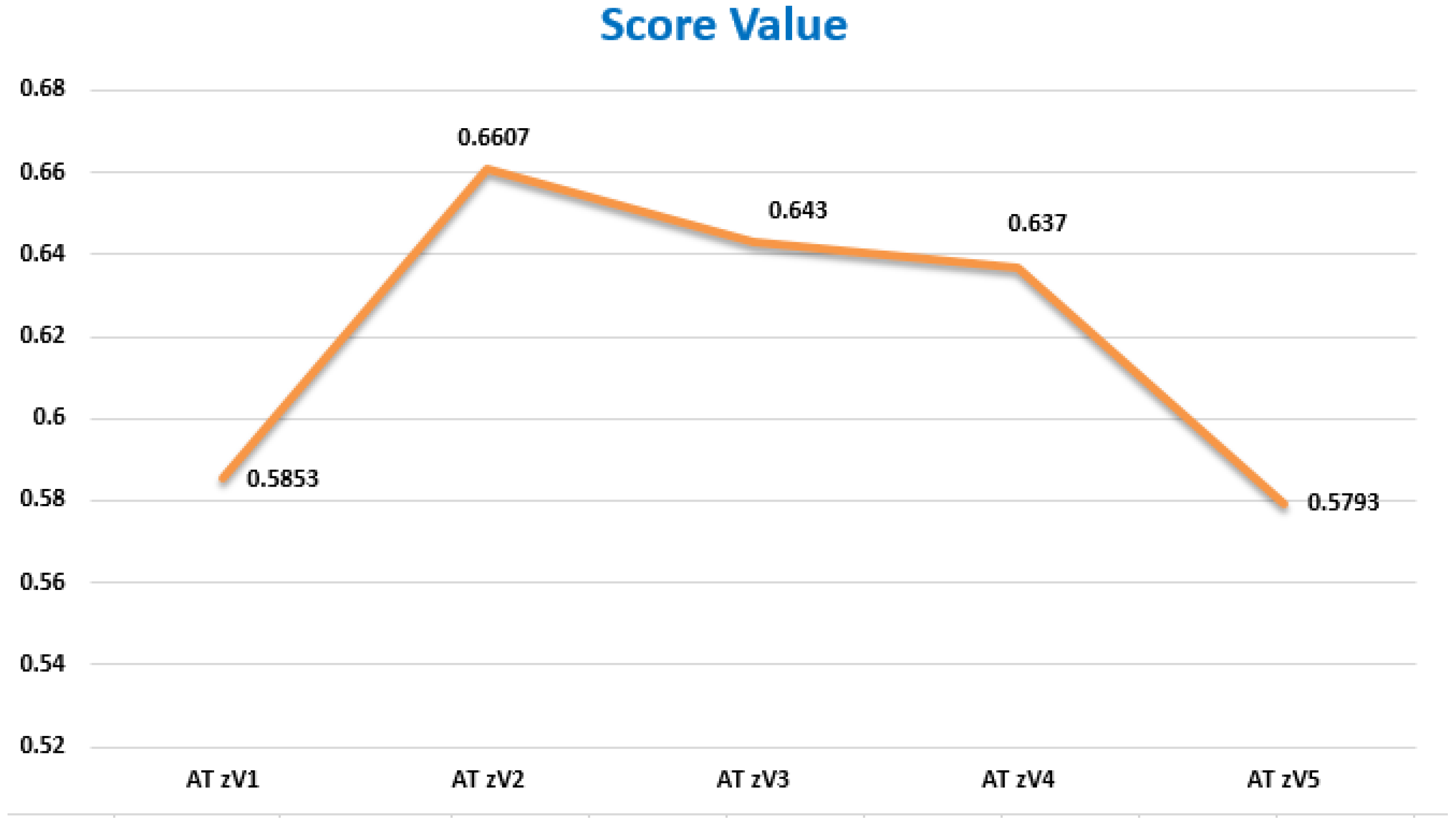
5.4. Sensitive Analysis

The robustness of the proposed approach under variations in key parameters was investigated through a sensitivity analysis. In particular, we examined the impact of altering controlling variables such as the Dombi parameter and weight allocations on the final ranking of alternatives. The objective was to determine whether small variations in input values result in significant changes in the outcome of decision-making. The results indicate that the proposed method exhibits a high level of stability. The rankings of alternatives remained largely consistent across a wide range of parameter changes, suggesting that the method is not overly sensitive to minor input fluctuations. This stability is crucial for real-world decision-making applications, where input data may be uncertain or imprecise. Overall, the research demonstrates that the suggested method is dependable and strong, which makes it appropriate for multi-criteria group decision-making issues in the actual world where parameter uncertainty is frequently unavoidable.

5.5. Advantages of the Suggested MAGDM Strategy

In this section, we outline a few benefits of our suggested MAGDM approach, which are as follows.

• To begin, the entire ordering principle on TzVNFNs is used in our suggested MAGDM technique, which is a broad category encompassing TNFNs, NFNs, and IVNFNs. Thus, real-valued NFNs, IVNFNs, and TNFNs are among the issues that can be solved using the algorithm suggested in the subclass context.
• Second, our suggested approach can always rank the two distinct TzVNFNs since the MAGDM algorithm incorporates the entire ordering principle. In other words, two distinct options (different performances according to separate criteria) will never be ranked as equal by the suggested MAGDM technique.
• Thirdly, by adjusting the Dombi variable, the $D{T}_n$ and $D{T}_{cn}$ oriented aggregating operator provides the benefit of making the aggregating procedure simpler. Flexibility may be achieved by altering the Dombi operator variable. Because of its adjustable parameters, it is adaptable to other t norms and t-conorms that are currently in use. We may modify the norm used for accumulation by changing the variable’s Dombi accumulation operator value, which also changes the parameter’s operational behavior. The primary benefit of this technique is that the evaluation takes into account the imprecision and ambiguity present in the real-time data.

6. Conclusions

For TzVNFNs, this paper presents a decision-making framework based on three Dombi-based accumulation operators namely TzVNFDWG, TzVNFDOWG, and TzVNFDHG. These operators enhance aggregation flexibility and satisfy essential mathematical properties through adjustable parameters. When applied to the selection of EV charging stations, the proposed TzVNFMAGDM model demonstrated improved performance under uncertain conditions. The integration of Dombi operators with neutrosophic modeling provides a more refined approach to handling ambiguity and expert hesitation in multi-attribute group decision-making.

Limitations and Future Scope

For TzVNFN, the suggested Dombi-based aggregation framework exhibits excellent flexibility, enhanced decision-making accuracy, and efficient uncertainty management through parameterized operations. But like many parameter-dependent models, its effectiveness depends on the Dombi control parameter selection, and domain-specific adjustment could be necessary to obtain the best results. Future studies may incorporate methods for managing conflicting expert opinions and extend the framework to dynamic decision-making environments. The model may also be extended to various fuzzy extensions, including q-rung ortho pair fuzzy environments and interval-valued neutrosophic sets.

References

1. Zadeh, L.A. Fuzzy sets. Inf. Control 1965, 8, 338–353. [Google Scholar] [CrossRef]
2. Atanassov, K.T. Intuitionistic fuzzy sets. Fuzzy Sets Syst. 1986, 20, 87–96. [Google Scholar] [CrossRef]
3. Smarandache, F. A Unifying Field in Logics. Neutrosophy: Neutrosophic Probability, Set and Logic; American Research Press: Rehoboth, DE, USA, 1999. [Google Scholar]
4. Ye, J. An extended TOPSIS method for multiple attribute group decision making based on single valued neutrosophic linguistic numbers. J. Intell. Fuzzy Syst. 2015, 28, 247–255. [Google Scholar] [CrossRef]
5. Chi, P.; Liu, P. An extended TOPSIS method for the multiple attribute decision making problems based on interval neutrosophic set. Neutrosophic Sets Syst. 2013, 1, 63–70. [Google Scholar]
6. Ali, M.; Hussain, Z.; Yang, M.-S. Hausdorff distance and similarity measures for single-valued neutrosophic sets with application in multi-criteria decision making. Electronics 2022, 12, 201. [Google Scholar] [CrossRef]
7. Dombi, J. A general class of fuzzy operators, the DeMorgan class of fuzzy operators and fuzziness measures induced by fuzzy operators. Fuzzy Sets Syst. 1982, 8, 149–163. [Google Scholar] [CrossRef]
8. Liu, P.; Liu, J.; Chen, S.-M. Some intuitionistic fuzzy Dombi Bonferroni mean operators and their application to multi-attribute group decision making. J. Oper. Res. Soc. 2018, 69, 1–24. [Google Scholar] [CrossRef]
9. Chen, J.; Ye, J. Some single-valued neutrosophic Dombi weighted accumulation Operators for multiple attribute decision-making. Symmetry 2017, 9, 82. [Google Scholar] [CrossRef]
10. Seikh, M.R.; Mandal, U. Intuitionistic fuzzy Dombi accumulation Operators and their application to multiple attribute decision-making. Granul. Comput. 2021, 6, 473–488. [Google Scholar] [CrossRef]
11. Shi, L.; Ye, J. Dombi Aggregation Operators of Neutrosophic Cubic Sets for Multiple Attribute Decision-Making. Algorithms 2018, 11, 29. [Google Scholar] [CrossRef]
12. Shao, Y.; Zhuo, J. Improved q-rung orthopair fuzzy line integral accumulation Operators and their applications for multiple attribute decision making. Artif. Intell. Rev. 2021, 54, 5163–5204. [Google Scholar] [CrossRef]
13. Deveci, M.; Gokasar, I.; Castillo, O.; Daim, T. Evaluation of metaverse integration of freight fluidity measurement alternatives using fuzzy Dombi EDAS model. Comput. Ind. Eng. 2022, 174, 108773. [Google Scholar] [CrossRef]
14. Jana, C.; Senapati, T.; Pal, M.; Yager, R.R. Picture fuzzy Dombi accumulation Operators: Application to MADM process. Appl. Soft Comput. 2019, 74, 99–109. [Google Scholar] [CrossRef]
15. Kumar, R.; Pamucar, D. A comprehensive and systematic review of multi-criteria decision-making (MCDM) methods to solve decision-making problems: Two decades from 2004 to 2024. Spectr. Decis. Mak. Appl. 2025, 2, 178–197. [Google Scholar] [CrossRef]
16. Asif, M.; Ishtiaq, U.; Argyros, I.K. Hamacher accumulation Operators for Pythagorean fuzzy set and its application in multi-attribute decision-making problem. Spectr. Oper. Res. 2025, 2, 27–40. [Google Scholar] [CrossRef]
17. Ali, A.; Ullah, K.; Hussain, A. An approach to multi-attribute decision-making based on intuitionistic fuzzy soft information and Aczel-Alsina operational laws. J. Decis. Anal. Intell. Comput. 2023, 3, 80–89. [Google Scholar] [CrossRef]
18. Meher, B.B.; Jeevaraj, S. Interval-valued Fermatean fuzzy Aczel-Alsina geometric accumulation Operators and their applications to group decision-making. Phys. Scr. 2024, 99, 095027. [Google Scholar] [CrossRef]
19. Sahoo, S.K.; Pamucar, D.; Goswami, S.S. A review of multi-criteria decision-making applications to solve energy management problems from 2010–2025: Current state and future research. Spectr. Decis. Mak. Appl. 2025, 2, 219–241. [Google Scholar] [CrossRef]
20. Naeem, M.; Ali, J. A novel multi-criteria group decision-making method based on Aczel-Alsina spherical fuzzy accumulation Operators: Application to evaluation of solar energy cells. Phys. Scr. 2022, 97, 085203. [Google Scholar] [CrossRef]
21. Khatter, K. Interval-valued trapezoidal neutrosophic set: Multi-attribute decision making for prioritization of non-functional requirements. J. Ambient Intell. Hum. Comput. 2021, 12, 1039–1055. [Google Scholar] [CrossRef]
22. Nayagam, V.L.; Jeevaraj, S.; Dhanasekaran, P. An improved ranking method for comparing trapezoidal intuitionistic fuzzy numbers and its applications to multicriteria decision making. Neural Comput. Appl. 2018, 30, 671–682. [Google Scholar] [CrossRef]
23. Meher, B.B.; Jeevaraj, S.; Alrasheedi, M. Dombi weighted geometric aggregation operators on the class of trapezoidal-valued intuitionistic fuzzy numbers and their applications to multi-attribute group decision-making. Artif. Intell. Rev. 2025, 58, 205. [Google Scholar] [CrossRef]
24. Bihari, R.; Jeevaraj, S.; Kumar, A. A new ranking principle for ordering generalized trapezoidal fuzzy numbers based on diagonal distance, mean and its applications to supplier selection. Soft Comput. 2023. [Google Scholar] [CrossRef]
25. Senapati, T.; Chen, G.; Mesiar, R.; Yager, R.R. Novel Aczel–Alsina operations-based interval-valued intuitionistic fuzzy aggregation operators and their applications in multiple attribute decision-making process. Int. J. Intell. Syst. 2022, 37, 5059–5081. [Google Scholar] [CrossRef]
26. Senapati, T.; Mesiar, R.; Simic, V.; Iampan, A.; Chinram, R.; Ali, R. Analysis of interval-valued intuitionistic fuzzy Aczel–Alsina geometric aggregation operators and their application to multiple attribute decision-making. Axioms 2022, 11, 258. [Google Scholar] [CrossRef]
Figure 1. Graphical representation of score value of alternatives final aggregated value.
Symmetry 17 01195 g001
Figure 2. Graphical representation of score value of alternatives final aggregated value.
Symmetry 17 01195 g002