Hydraulic Flow Patterns in an On-Site Wastewater Treatment Unit Under Various Operating Conditions

Abstract

The role of on-site wastewater treatment (OSWT) is increasingly important for water reuse and local sustainability, but treatment efficiency is highly dependent on hydraulic behavior and mixing. This study used validated CFD simulations and tracer experiments to analyze flow patterns and mixing performance in a six-zone OSWT unit under different operational scenarios, including inflow, aeration, recirculation, combined mechanisms, and closed-loop operation without inflow. The results show that influent flow is essential for maintaining convective transport and system-wide momentum, while aeration and recirculation enhance local mixing, but cannot fully overcome geometric dead zones. The combined use of inflow, aeration, and recirculation achieved the highest mixing efficiency and minimized the dead volume, whereas scenarios lacking inflow exhibited severe stagnation and expanded dead zones. These findings highlight the need to integrate hydraulic interventions with thoughtful reactor design to ensure effective and resilient small-scale wastewater treatment systems.

1. Introduction

The European Union’s Regulation 2020/741 establishes comprehensive standards for the safe reuse of treated wastewater, promoting resource efficiency and sustainability while safeguarding public health and the environment [1]. Based on the legislation, agglomerations with fewer than 1000 population equivalent (PE) are not mandated to be part of centralized wastewater collection systems; decentralized sewage collection and treatment approaches are prioritized in such cases [2,3]. Looking deeper, spatial rural patterns serve as a critical parameter for supporting decision-making in the implementation of decentralized wastewater systems, ensuring their economic feasibility by aligning infrastructure design with population distribution and settlement characteristics [4].

For even smaller communities or households, the legislation permits the installation of on-site small-capacity wastewater treatment systems, tailored to the specific needs of the location. Although a wide variety of such systems are available on the market, the majority rely on aerobic biodegradation processes, where air blowers provide the necessary oxygen, consuming energy in the process. The operation of these air blowers varies in complexity depending on the manufacturer, ranging from simple time-based controls to advanced automation systems utilizing dissolved oxygen sensors in the bioreactor [5]. Mirra et al. (2020) [6] confirmed that energy use in OSWT systems can be optimized using a simple water level sensor. Their results demonstrated that during periods without wastewater generation, the oxygen uptake rate (OUR) in the reactor remained low (0.0007–0.0015 mg/L·s), requiring minimal oxygen supply. However, when wastewater entered the system and water levels rose, oxygen demand increased significantly, and the OUR reached 0.0040–0.0063 mg/L·s, depending on the type and quantity of the incoming substrate [6].

However, aeration is not only responsible for satisfying the biological processes’ oxygen demand, but also plays a key role in mixing within the treatment unit [7]. Effective mixing ensures uniform distribution of microorganisms, substrates, and dissolved oxygen, which is essential for maintaining process stability and preventing sludge settlement or the formation of dead zones [8]. The hydraulic behavior of OSWT units is fundamental to ensuring effective pollutant removal, stable operation, and long-term reliability. These systems, which typically serve single households or small communities, must cope with highly variable hydraulic and organic loads due to fluctuating household activities, making their design and operation particularly challenging [9,10].

Hydraulic performance in these units is influenced by several factors, including the degree of pipe filling, slope, pipe diameter, and the configuration of inlets and outlets. Maintaining an optimal filling ratio (generally between 0.5 and 0.75) is essential, as it ensures a proper balance between water and air, promotes the transport of solids, and reduces the risk of sedimentation or blockages [11]. Hydraulic loading directly affects the retention time, which is a critical parameter for treatment efficiency. Within the treatment unit, the hydraulic linkage of compartments such as settlers, reactors, and filters, as well as precise water level regulation, are crucial for smooth operation and achieving the desired effluent quality [12]. The magnitude of hydraulic loading determines the residence time of wastewater in each unit, which, in its turn, influences organic matter degradation, sedimentation, and biological activity. Excessive loading could result in incomplete treatment, while underloading leads to underutilized systems and lower energy efficiency [13].

Traditional hydraulic design methods frequently oversimplify the actual flow conditions, neglecting the effects of complex geometries, multiphase flows, turbulence, and the interplay between biological and physical processes. In recent years, computational fluid dynamics (CFD) simulations have become increasingly important in the design and optimization of wastewater treatment systems, as they enable detailed analysis of flow patterns, vortices, dead zones, short-circuiting, and solids distribution under realistic conditions [14,15]. CFD modeling can help identify hydraulic issues, improve unit design, optimize energy use, reduce operational costs, and enhance treatment efficiency. However, the literature indicates that CFD-based design and diagnostics are not yet widespread for individual, small-scale treatment units, mainly due to a lack of validated models, limited laboratory and field data, and the complexity of biological processes [16].

Maintaining a high degree of mixedness within a reactor chamber of an on-site wastewater treatment unit is essential for effective treatment performance. Inadequate mixing could lead to operational issues such as sludge settling, reduced contact between microorganisms and contaminants, and uneven distribution of chemicals, all of which can compromise treatment efficiency and stability [17]. The coherent structure concept helps improve the understanding and optimization of flow patterns and mixing dynamics within small-capacity wastewater treatment units. By identifying and analyzing coherent flow structures—such as recirculation zones and eddies—engineers can predict areas prone to dead zones or hydraulic short-circuiting, which are particularly problematic in compact reactor chambers [17].

Current studies often overlook the dynamic nature of flow and mixing under real operational events such as peak inflow shocks, intermittent aeration, or varied recirculation. This work addresses shortcomings in understanding how these realistic perturbations impact internal hydraulics, dead zones, and mixing—factors directly tied to treatment reliability and design optimization. The aim of this research is to perform detailed simulations to reveal small-scale hydraulic and mixing phenomena within an on-site wastewater treatment unit, with a particular focus on identifying well-mixed and poorly mixed zones. By mapping these zones, the study seeks to provide insights that can guide the optimization of reactor design and operational strategies, ultimately enhancing treatment efficiency and reliability in small-capacity systems.

2. Materials and Methods

2.1. Governing Equations of CFD Simulation

2.1.1. 3D Flow with Turbulence Closure

Three-dimensional flow simulations in small-capacity wastewater treatment units are conducted using the Reynolds-averaged Navier–Stokes (RANS) framework with k–ε turbulence closure [18,19]. The RANS k–ε turbulence model was chosen for its balance of computational efficiency and validated accuracy in simulating turbulent flows and mixing in environmental and engineering-scale reactors, including wastewater treatment systems. This model effectively captures the key features of vortex formation, dead zones, and mixing in compartmentalized geometries, which are essential for accurate representation of OSWT hydrodynamics. In this context, aeration and bubble formation are modeled using Euler–Euler multiphase approach, where both the liquid and gas phases are treated as interpenetrating continua, enabling detailed simulation of phase interactions, bubble dynamics, and their impact on mixing and oxygen transfer within the reactor [20]. This methodology provides a robust and physically realistic toolset for resolving intricate hydrodynamics and mixing behavior essential for optimizing small-scale wastewater treatment performance. Numerical calculations are described below.

Phase continuity equations:

For liquid phase ($l$) and gas phase ($g$):

$${\displaystyle \frac{\partial }{\partial t}}({\alpha }_k{\rho }_k)+\nabla \cdot ({\alpha }_k{\rho }_k{\mathbf{u}}_k)=0 (k=l,g)$$

(1)

${\alpha }_k$: volume fraction of phase $k$ (${\alpha }_l+{\alpha }_g=1$)

${\rho }_k$: density of phase $k$

${\mathbf{u}}_k$: velocity vector of phase $k$

Phase momentum equations:

$$\begin{array}{r}{\displaystyle \frac{\partial }{\partial t}}({\alpha }_k{\rho }_k{\mathit{u}}_k)+\nabla \cdot ({\alpha }_k{\rho }_k{\mathit{u}}_k{\mathit{u}}_k)=\\ -{\alpha }_k\nabla p+\nabla \cdot \left({\alpha }_k{\mu }_{\mathit{eff},k}\left[\nabla {\mathit{u}}_k+(\nabla {\mathit{u}}_k{)}^T\right]\right)+{\alpha }_k{\rho }_k\mathit{g}+{\mathit{M}}_k\end{array}$$

(2)

$p$: shared pressure field

$\mathbf{g}$: gravity vector

${\mathbf{M}}_k$: interphase momentum transfer

${\mu }_{\mathit{eff},k}$: effective viscosity

Turbulence (k–ε) model:

Solved for the mixture phase to model liquid-phase turbulence:

Turbulent kinetic energy ($k$):

$${\displaystyle \frac{\partial }{\partial t}}({\rho }_{m}k)+\nabla \cdot ({\rho }_m{\mathbf{u}}_{m}k)=\nabla \cdot \left({\displaystyle \frac{{\mu }_{\mathrm{t},m}}{{\sigma }_k}}\nabla k\right)+G_{k,m}-{\rho }_m\epsilon$$

(3)

Dissipation rate ($\epsilon$):

$${\displaystyle \frac{\partial }{\partial t}}({\rho }_m\epsilon )+\nabla \cdot ({\rho }_m{\mathbf{u}}_m\epsilon )=\nabla \cdot \left({\displaystyle \frac{{\mu }_{\mathrm{t},m}}{{\sigma }_{\epsilon }}}\nabla \epsilon \right)+C_{1\epsilon }{\displaystyle \frac{\epsilon }{k}}{G}_{k,m}-C_{2\epsilon }{\rho }_m{\displaystyle \frac{{\epsilon }^2}{k}}$$

(4)

${\rho }_m={\alpha }_l{\rho }_l+{\alpha }_g{\rho }_g$: mixture density

${\mathbf{u}}_m=\frac{{\alpha }_l{\rho }_l{\mathbf{u}}_l+{\alpha }_g{\rho }_g{\mathbf{u}}_g}{{\rho }_m}$: mixture velocity

$G_{k,m}={\mu }_{\mathrm{t},m}\left(\nabla {\mathbf{u}}_m+(\nabla {\mathbf{u}}_m{)}^T\right):\nabla {\mathbf{u}}_m$: turbulence production

${\mu }_{\mathrm{t},m}=C_{\mu }{\rho }_m{\displaystyle \frac{k^2}{\epsilon }}$: turbulent viscosity

The mode constants are as follows: $C_{\mu }=0.09$, $C_{1\epsilon }=1.44$, $C_{2\epsilon }=1.92$, ${\sigma }_k=1.0$, ${\sigma }_{\epsilon }=1.3$.

Interphase momentum transfer (${\mathrm{M}}_k$):

Drag force dominates in bubble-liquid systems:

$${\mathbf{M}}_l=-{\mathbf{M}}_g=K_{lg}({\mathbf{u}}_g-{\mathbf{u}}_l)$$

(5)

Drag coefficient ($K_{lg}$):

$$K_{lg}={\displaystyle \frac{3}{4}}{\alpha }_g{\alpha }_l{\rho }_l{\displaystyle \frac{C_D}{d_b}}\Vert {\mathbf{u}}_g-{\mathbf{u}}_l\Vert$$

(6)

$C_D$: drag coefficient

$d_b$: bubble diameter

A constant representative bubble diameter of 1 mm was assumed, in accordance with the specifications of the actual aeration system. It is important to note that this value represents the initial bubble size at the point of entry into the system.

2.1.2. Residence Time Distribution Analysis

Numerical residence time distribution (RTD) analysis was performed using a tracer that is physically identical to the main water flow, ensuring that the tracer follows the same hydrodynamic pathways as the bulk liquid [21,22]. Initially, a steady-state simulation was conducted with a single water phase to establish the baseline flow field. Subsequently, the simulation was switched to transient mode, and from time zero, a second, “labelled” water phase (tracer) was continuously injected at the inlet. Simultaneously, the volume fraction of this labelled water (water 2) was monitored at the outlet, allowing for the determination of the cumulative distribution function, F(t), of the tracer. This approach provides a detailed and realistic assessment of the reactor’s hydraulic behavior, enabling the identification of dead zones, short-circuiting, and the overall mixing efficiency within the treatment unit [23]. In our investigation, the cumulative outlet signal F(t) was detected, that is, the cumulative fraction of the tracer exiting the system, as per the standard RTD protocols for step-type tracer applications. The distribution function E(t) can be calculated as follows:

$$E(t)={\displaystyle \frac{dF\left(t\right)}{dt}}$$

(7)

The mean residence time ($\overline{t}$) and the variance (${\sigma }^2$) can be calculated as follows:

$$\overline{t}={\int }_0^{\infty } tE(t) dt$$

(8)

and

$${\sigma }^2={\int }_0^{\infty } (t-\overline{t}{)}^{2}E(t) dt$$

(9)

For the physical residence time distribution (RTD) test, a sodium chloride (NaCl) solution was used as a conservative tracer [24]. Baseline electrical conductivity was first measured at the effluent zone to establish the initial conditions. Following this, a NaCl solution was introduced into the system, resulting in increased conductivity at the measurement point as the tracer passed through. By continuously monitoring the conductivity changes over time at these locations, the progression and dispersion of the tracer could be tracked, enabling the calculation of local and overall residence time characteristics and the identification of well-mixed and poorly mixed zones within the treatment unit. The field measurement data served as validation for the CFD study, ensuring that the simulated hydraulic and mixing patterns accurately reflected real system behavior [25].

In the analysis, normalized time (denoted as θ) was applied, defined as the ratio of actual time (t) to the mean residence time (τ):

$$\theta ={\displaystyle \frac{t}{\tau }}$$

(10)

This dimensionless scaling allows comparison across different flow conditions or system sizes. The response function uses min–max normalized conductivity, calculated as follows:

$${\kappa }^{\ast }={\displaystyle \frac{\kappa -{\kappa }_{min}}{{\kappa }_{max}-{\kappa }_{min}}},$$

(11)

where κ is the measured conductivity.

2.1.3. Mixing and Mixedness

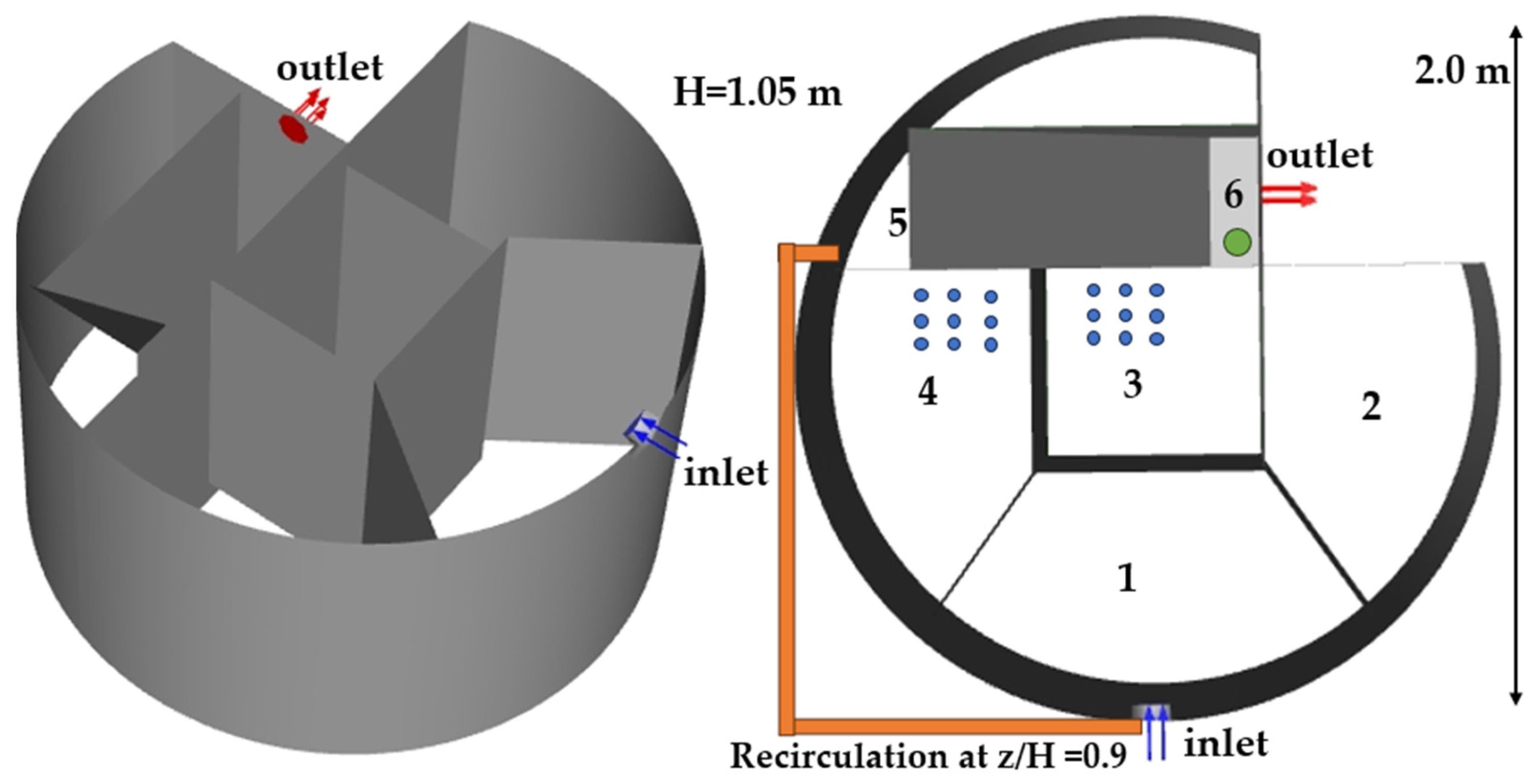
A commonly used method to quantitatively assess mixing and mixedness in a reactor compartment is the calculation of the degree of mixing (or the mixing index) based on the variance of the tracer concentration field [26]. First, the volume-averaged tracer concentration is calculated for the entire compartment. Then, for each computational cell, the local tracer volume fraction is determined. The degree of mixing at a given time can be expressed by the normalized variance of the tracer concentration:

$$Mixing Index=1-{\displaystyle \frac{{\sum }_{i=1}^N{V}_i{\left(C_i-\overline{C}\right)}^2}{{\sum }_{i=1}^N{V}_i{\left(\overline{C}\right)}^2}}$$

(12)

V_i: volume of cell i

C_i: scalar volume fraction in cell i

$\overline{C}$: volume-averaged scalar concentration

A mixing index value close to 1 indicates nearly perfect mixing (homogeneous distribution). A value near 0 indicates poor mixing (high concentration gradients). This method allows for a quantitative, time-resolved evaluation of how quickly and thoroughly the tracer (and thus the fluid) becomes evenly distributed within the compartment, providing a robust measure of mixing performance.

All CFD simulations were run in OpenFOAM v24. Convergence was assumed when the normalized residuals for continuity, momentum, and turbulence variables dropped below 10⁻⁴. Time-stepping used adaptive sizes, ensuring Courant numbers remained below 1.

2.2. Study Site

The wastewater treatment unit (Figure 1) operates through a sequential flow process across six distinct zones with a total volume of approximately 3.2 m³. Wastewater enters through the inlet at near-surface into Zone 1 (0.76 m³), which serves as a balancing chamber and receives recirculated flow from Zone 5. From Zone 1, the flow moves to Zone 2 (0.59 m³), an anaerobic zone where organic matter begins decomposition without aeration.

The partially treated water then progresses to Zone 3 (0.42 m³), the first aerated aerobic zone where biological oxidation occurs. Flow continues to Zone 4 (0.59 m³), another aerated aerobic zone that further processes the wastewater. The treated water then moves to Zone 5 (0.54 m³), an aerobic zone that provides final biological treatment while also sending recirculated flow back to Zone 1 to enhance treatment efficiency (

Table 1. Basic data on the onsite wastewater treatment unit.

Zone No.	Volume [m3]	Aerated	Recirculation	Role
1	0.76	No	From zone 5	Balancing
2	0.59	No	-	Anaerobic
3	0.42	Yes	-	Aerobic
4	0.59	Yes	-	Aerobic
5	0.54	No	To zone 1	Aerobic
6	0.26	No	-	Settling

). Zone 5, while not mechanically aerated, maintains aerobic conditions as residual oxygen from upstream aerated compartments sustains dissolved oxygen levels in the range of 1.2–1.4 mg/L, based on the authors’ previous experience. Thus, despite the absence of direct aeration, Zone 5 can support aerobic biological processes due to effective oxygen carryover. Recirculation from Zone 5 to Zone 1 is achieved by an external pump operating at 0.4 m³/d; the flow rate can be adjusted by a variable-speed drive. Aeration uses three diffusers located at the base of Zones 3 and 4, each supplied at rates of 2.6 m³/h via a common air distributor. Outlet conductivity is monitored by a continuous sensor probe positioned at the effluent pipe.

Finally, the water enters Zone 6 (0.26 m³), a non-aerated settling zone where suspended solids separate before the clarified effluent exits through the outlet. This design combines anaerobic, aerobic, and settling processes with recirculation to achieve effective wastewater treatment in a compact cylindrical configuration.

2.3. Operational Scenarios

Investigating scenarios A–E under the specified conditions (

Table 2. Operational scenarios.

Scenario	Inflow	Aeration	Recirculation
A	ON	OFF	OFF
B	ON	ON	OFF
C	ON	OFF	ON
D	ON	ON	ON
E	OFF	ON	ON

)—including an average daily load of 400 L/d with peak shocks such as a 4 L/min bathtub release (5 min), aeration rates of 2.6 m³/h, and recirculation of 0.4 m³/d—is essential for understanding real-world hydraulic behavior in on-site wastewater treatment.

Scenario A (inflow only) isolates natural convective mixing during extreme hydraulic events, revealing baseline performance without mechanical assistance. Scenario B (inflow + aeration) quantifies how aeration enhances mixing across tested rates, while Scenario C (inflow + recirculation) evaluates recirculation’s standalone impact on flow symmetry. Scenario D (inflow + aeration + recirculation) identifies synergies or redundancies between mechanisms at combined operational settings, and Scenario E (aeration + recirculation, no inflow) tests stability during low-demand periods, which can occur at nighttime. This systematic approach, grounded in pilot-verified baselines, directly informs energy optimization, dead zone prevention, and system resilience across diurnal load variations.

2.4. Mesh Quality and Independence Analysis

Mesh quality was visually and quantitatively evaluated to ensure the simulation’s reliability, focusing on the metric of cell equiangle skew. The coarse mesh consisted of 401,480 tetrahedral elements; the practical mesh used 722,664 elements, whereas the fine mesh consisted of 1,003,700 elements. Figure 2 shows that the coarse mesh peaked at a probability of about 0.30, with a cell equiangle skew around 0.42. In comparison, both the practical and fine meshes peaked higher, at approximately 0.37 and 0.38, respectively, with their skew values centered around 0.38. This demonstrates that the practical and fine meshes have lower skew and higher quality, with no significant difference between them, making the practical mesh the preferred choice.

Mesh independence analysis was conducted using three mesh densities to ensure solution accuracy and computational efficiency. The results in

Table 3. Mesh independence analysis: comparison of the key volume-averaged hydrodynamic parameters for three mesh densities.

Mesh Density	No. of Elements	Volume-Averaged Mixing Index	Turbulent Kinetic Energy (TKE)	Turbulent Dissipation Rate (ε)
Coarse	401,480	0.612	0.283	0.375
Practical	722,664	0.597	0.269	0.333
Fine	1,003,700	0.596	0.267	0.332

demonstrate that all key hydrodynamic parameters (mixing index, turbulent kinetic energy, and dissipation rate) converge with increasing mesh refinement, showing less than 1% difference between the practical and fine meshes.

The close agreement between the practical and fine mesh solutions, with relative differences below 1% for all the monitored parameters, confirms that mesh independence was achieved at the practical mesh density. The systematically elevated values from the coarse mesh indicate insufficient spatial resolution to accurately resolve the turbulent flow structures and mixing processes. Based on these results, the practical mesh was selected for all subsequent simulations as it provides the optimal balance between computational accuracy and efficiency.

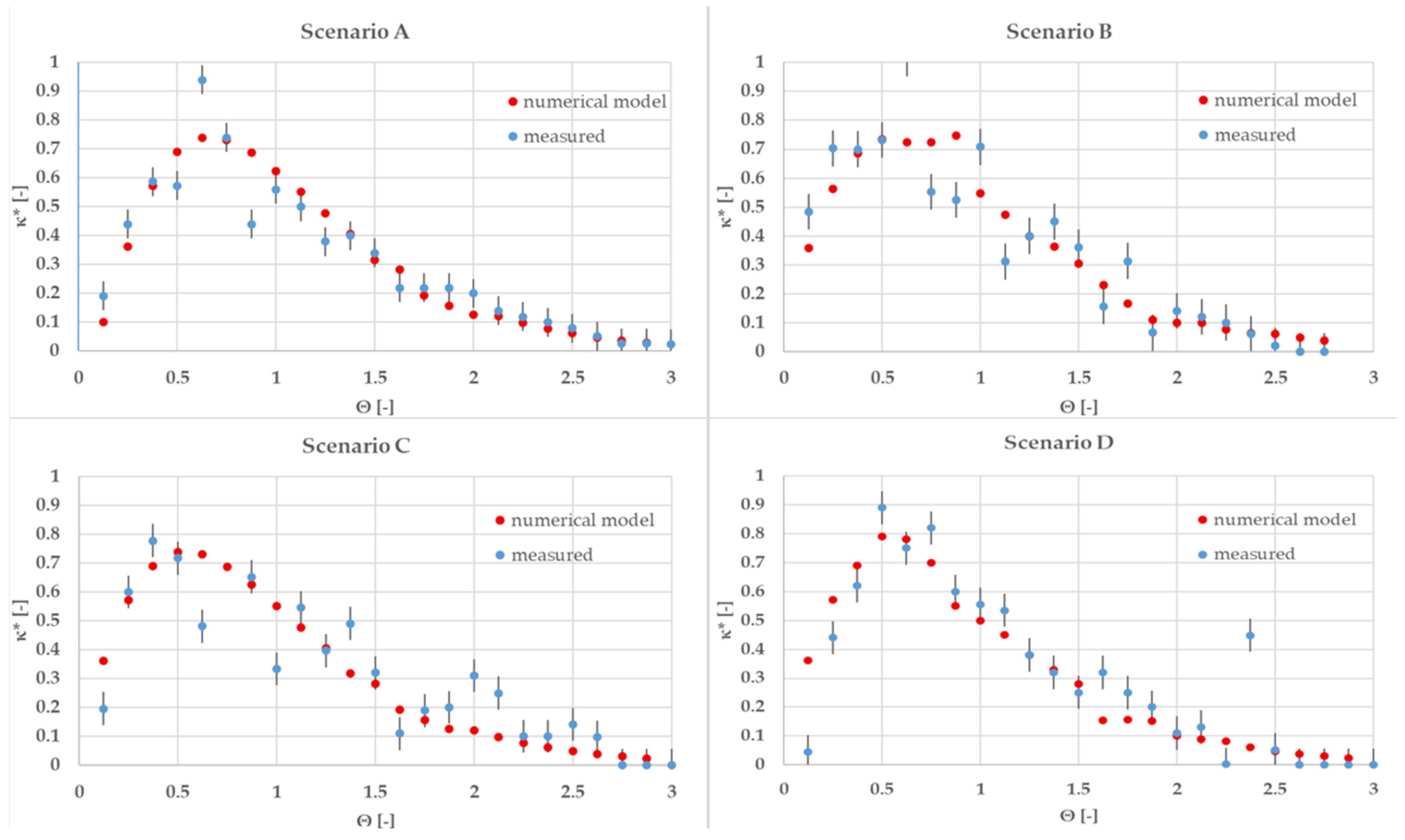
3. Residence Time Analysis—Model Verification

The exit age distribution functions E(t) for Scenarios A–D are presented in Figure 3, with normalized time on the x-axis and the min–max normalized conductivity on the y-axis. Here, E(t) was obtained by differentiating the cumulative distribution F(t), enabling clearer comparison of tracer breakthrough and hydrodynamic differences between the scenarios. Experimental measurements are shown with error bars reflecting variance from replicate tests. While early deviations appear due to practical limitations in capturing the initial salt front—such as probe response lag and the difficulty of promptly detecting tracer inflow—scenarios involving aeration and/or recirculation (B–D) reveal broader and earlier E(t) peaks compared to the inflow-only scenario (A), highlighting the accelerating effect of these mechanisms on mixing and short-circuiting. As local turbulence and recirculation-induced flow redistribution intensify, experimental data show increased variability and non-monotonicity at early and intermediate normalized times, especially under combined operation (D), due to stronger hydraulic perturbations and the formation of preferential flow paths. Overall, these profiles demonstrate that while aeration and recirculation significantly alter mixing dynamics—leading to earlier tracer breakthroughs and wider residence time distributions—operational complexity and measurement uncertainties increase, particularly at the onset of each experiment.

Residence time characteristics for the four operational scenarios were evaluated directly from the E(t) curves, where the mean residence time and variance were calculated based on Equations (8) and (10), as detailed in the methodology. Scenario A (inflow only) yielded a baseline residence time of 13.16 h, with the experimental and simulated E(t) curves exhibiting nearly identical unimodal peaks and symmetric shapes, reflecting a well-mixed system and indicating strong model–measurement agreement throughout the entire normalized time range (deviation < 2%). For Scenario B (inflow + aeration), the mean residence time was reduced to τ = 12.3 h (−6.5% from baseline), and the E(t) peak broadened and shifted left, signifying earlier tracer breakthrough and an increase in short-circuiting due to turbulence-induced preferential pathways; notable discrepancies appeared near the initial rise (θ < 0.5), likely due to both aeration-driven mixing and practical difficulties in capturing the instant tracer arrival.

Scenario C (inflow + recirculation) exhibited a further reduction to τ = 11.3 h (−14% vs. A), with the E(t) curve revealing multiple wider peaks and flattened regions, indicating a mix of accelerated transport (bypassing) through newly formed recirculation channels and sustained stagnation zones. Scenario D (inflow + aeration + recirculation) presented the shortest mean residence time at τ = 9.4 h (−29% from baseline).

4. Results and Discussion

4.1. Mixing Pattern Analysis

The analysis of mixing indices across the six compartments reveals distinct patterns influenced by operational mechanisms (

Table 4. Mixing indices in different compartments and scenarios.

Zone	Scenario A	Scenario B	Scenario C	Scenario D	Scenario E
1	0.62 ± 0.08	0.65 ± 0.06	0.89 ± 0.03	0.93 ± 0.02	0.78 ± 0.07
2	0.58 ± 0.09	0.67 ± 0.07	0.71 ± 0.05	0.86 ± 0.04	0.49 ± 0.11
3	0.53 ± 0.11	0.85 ± 0.04	0.63 ± 0.08	0.91 ± 0.03	0.69 ± 0.09
4	0.49 ± 0.12	0.88 ± 0.03	0.59 ± 0.09	0.94 ± 0.02	0.72 ± 0.08
5	0.47 ± 0.13	0.87 ± 0.04	0.83 ± 0.05	0.95 ± 0.01	0.81 ± 0.06
6	0.41 ± 0.15	0.52 ± 0.10	0.48 ± 0.11	0.69 ± 0.07	0.22 ± 0.017

). In Scenario A (inflow only, τ = 13.16 h), mixing efficiency decreases progressively downstream, with Zone 1 at 0.62 (±0.08) and Zone 6 dropping to 0.41 (±0.15), indicating severe stratification and a dead zone in the final compartment. Scenario B (aeration in Zones 3–5, τ = 12.3 h) significantly improves homogeneity in aerated zones—Zone 3 jumps to 0.85 (±0.04), Zone 4—to 0.88 (±0.03), and Zone 5—to 0.87 (±0.04), demonstrating aeration’s localized efficacy, though non-aerated Zones 1–2 and 6 show marginal gains (≤0.67).

Scenario C (recirculation Zone 5 → 1, τ = 11.3 h) maximizes mixing at flow redistribution points: Zone 1 surges to 0.89 (±0.03) and Zone 5 to 0.83 (±0.05), validating recirculation’s targeted impact, but intermediate Zones 2–4 and Zone 6 remain suboptimal (≤0.71). Scenario D (combined mechanisms, τ = 9.4 h) achieves a synergistic enhancement: Zone 1 (0.93 ± 0.02) and Zone 5 (0.95 ± 0.01) feature near-perfect homogeneity, while aerated Zones 3–4 exceed 0.90, and even Zone 6 improves to 0.69 (±0.07). Critically, Zone 6 consistently underperforms across all scenarios (peak of 0.69 in D vs. 0.41 in A), confirming its geometric limitations as a persistent dead zone. The 29% residence time reduction in Scenario D (9.4 h vs. 13.16 h in A) correlates with optimal mixing efficiency (mean index of 0.88 vs. 0.52 in A), proving combined aeration and recirculation resolve trade-offs between throughput and mixing quality—except in Zone 6, which requires dedicated interventions such as baffle redesign or extended aeration.

In Scenario E, where the system operates with recirculation (Zone 5 → Zone 1) and aeration (Zones 3 and 4) but no inflow, mixing efficiency significantly deteriorates compared to Scenario D (which included the inflow). The closed-loop operation eliminates the hydraulic driving force provided by the inflow, reducing global momentum and causing severe stagnation. Zone 1 maintains moderate homogeneity (0.78 ± 0.07) due to recirculated flow from Zone 5, while Zone 5 itself retains a relatively high index (0.81 ± 0.06) as the recirculation source. However, Zones 3 and 4—though aerated—drop by 24–23% (to 0.69 ± 0.09 and 0.72 ± 0.08, respectively) due to diminished fluid exchange. Critically, Zone 2 collapses to 0.49 ± 0.11 (−43% vs. Scenario D) without inflow-driven fluid renewal, and Zone 6 becomes a hydraulic dead zone (0.22 ± 0.17, −68%), isolated from recirculation paths and lacking inflow-induced mixing. This confirms that inflow is essential for system-wide momentum: without it, recirculation and aeration only sustain localized mixing in directly connected zones (1, 3–5), while downstream compartments stagnate. The mean mixing index falls to 0.52 (vs. 0.88 in Scenario D), and dead zones likely exceed 10% of the volume, highlighting inflow’s irreplaceable role in preventing fluid stagnation and optimizing reactor performance.

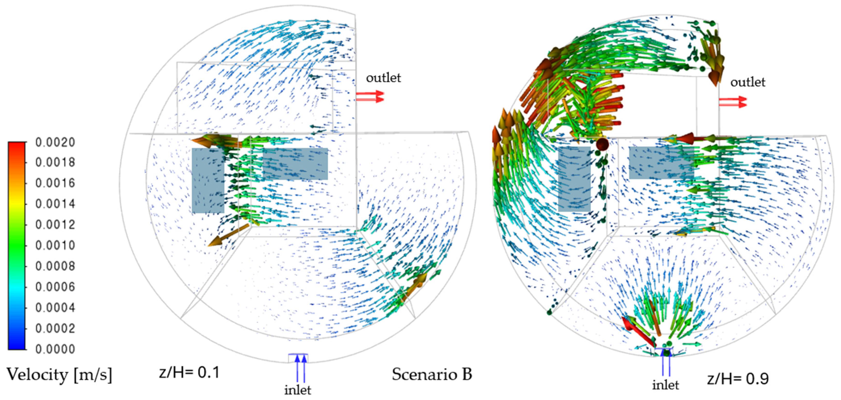
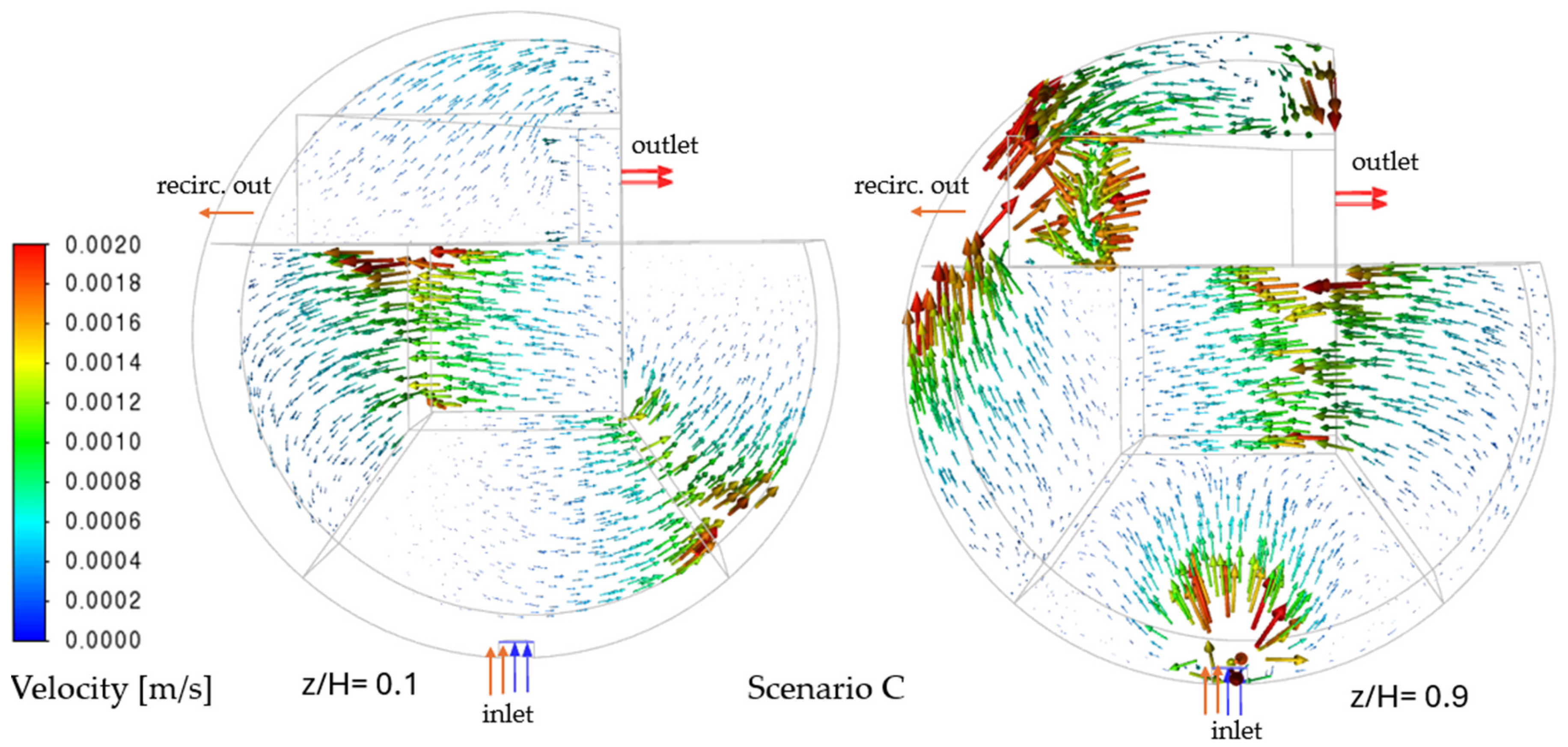
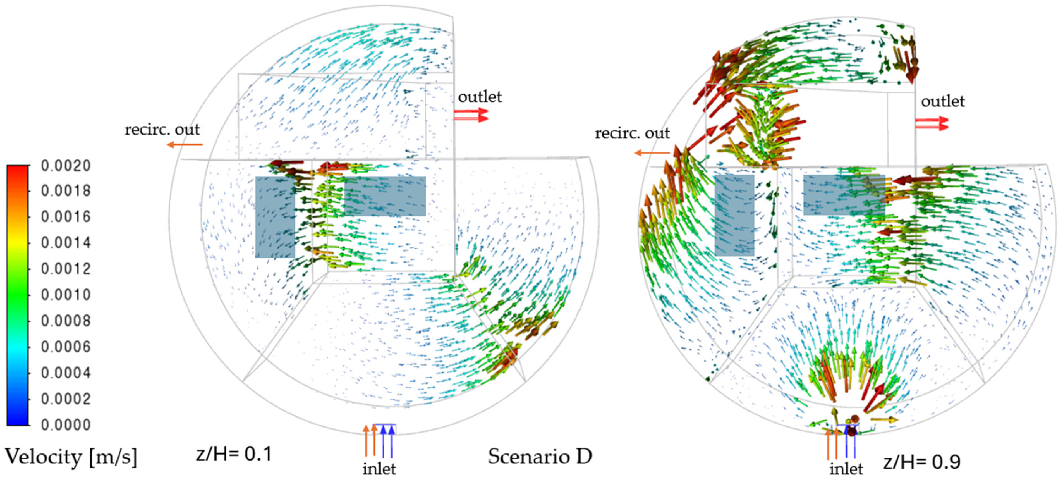
4.2. Flow Field Analysis Across the Scenarios

The flow fields across Scenarios A–E exhibit distinct hydrodynamic behaviors, visualized through velocity contours and trajectory patterns. In Scenario A (Figure 4), the velocity field is uniformly low-magnitude (0.001–0.0016 m/s), indicating stable flow from Zone 1 (inflow) to Zone 6 (outflow).. The absence of aeration or recirculation allows geometric constraints to dominate, causing a velocity gradient that decays toward Zone 6 (0.0002–0.0004 m/s), indicative of incipient stagnation.

Scenario B (aeration in Zones 3 and 4) introduces localized momentum, accelerating flow in aerated zones to 0.0014–0.0018 m/s (Figure 5). These vortices cause some particle paths to accelerate and recirculate within aerated compartments, while regions without aeration (Zones 1–2, 6) remain comparatively stagnant. The divergence spikes in aerated zones (+0.12 s⁻¹) confirm source-like behavior, explaining the E(t) curve’s early rise.

Scenario C (recirculation Zone 5 → 1) redistributes momentum, forming a high-velocity jet (0.0018 m/s) at Zone 1 (Figure 6). This creates a helical flow near the recirculation inlet, but Zones 2–4 develop stagnation pockets (velocity ≤ 0.0006 m/s). The recirculation-driven flow is incomplete without inflow, causing particle trajectories to loop indefinitely in Zones 1 and 5 but collapse in Zone 6.

Scenario D (combined inflow, aeration, recirculation) achieves global momentum (0.0010–0.0018 m/s) through synergistic effects. Vortices in Zones 3–5 merge with recirculation-driven jets, with a little oscillation before exiting (Figure 7). Despite this, Zone 6 remains a divergence sink (−0.08 s⁻¹), trapping 4.5% of the fluid volume.

Scenario E (no inflow, recirculation + aeration) collapses system-wide flow (Figure 8): velocities decay to ≤ 0.0006 m/s except near aerators (0.0012 m/s). Particle trajectories form isolated limit cycles in Zones 1, 3–5, while Zones 2 and 6 stagnate (0.0002 m/s), confirming inflow’s role as the primary hydraulic driver.

The hydrodynamic patterns observed across Scenarios A–E demonstrate critical interactions between operational mechanisms and geometric constraints, with implications for on-site wastewater treatment design. The persistent dead zone in Zone 6 (velocity ≤ 0.0006 m/s, mixing index ≤ 0.69) across all the scenarios underscores the dominance of geometric limitations over operational adjustments. This aligns with Lima et al.’s [26] findings that reactor geometry fundamentally determines the fluid flow structures, and strong three-dimensional effects were observed in a rectangular tank.

A summary of key hydraulic indicators for all the operational scenarios is shown in

Table 5. Summary table of the scenario results.

Scenario	Operation	Mean Residence Time, τ (h)	Mean Mixing Index (Full Reactor)	Zone 6 Mixing Index	Max Velocity (m/s, Main Zones)
A	Inflow only	13.16	0.52 (±0.08)	0.41 (±0.15)	0.0016
B	Inflow + aeration	12.3	0.62 (±0.07)	0.67 (±0.13)	0.0018
C	Inflow + recirculation (5 → 1)	11.3	0.67 (±0.06)	0.53 (±0.12)	0.0018
D	Inflow + aeration + recirculation	9.4	0.88 (±0.04)	0.69 (±0.07)	0.0018
E	Aeration + recirculation, no inflow	— *	0.52 (±0.10)	0.22 (±0.17)	0.0012 (local)

* without inflow, there is no outflow, resulting an infinite residence time.

, facilitating direct comparison of residence time, mixing, velocity field, and dead volume performance.

Aeration’s vortical structures (curl > 0.12 s⁻¹) enhanced mixing in Zones 3–5 (mixing index: 0.85–0.88) but accelerated short-circuiting, reducing effective residence time by 6.5%—a phenomenon that reflects how vigorous local mixing can unintentionally create preferential fast-flow pathways, allowing a larger fraction of incoming fluid to bypass the intended treatment volume and exit prematurely before complete processing. Recirculation’s high-velocity jet (0.0018 m/s) in Zone 1 improved local homogeneity (index: 0.89) but starved mid-reactor zones (Zones 2–4, velocity: ≤0.0006 m/s). Scenario D proved that combined operations counteract individual mechanism flaws, though Zone 6’s stagnation persisted. This reflects the conclusion by Oliveira et al. (2020) that integrated inflow–aeration–recirculation systems convert plug flow systems to completely stirred reactors [27].

Scenario D, while hydraulically optimal, entails higher energy consumption due to the continuous operation of both the recirculation pump and aerators. A trade-off analysis for blower and pump duty vs. marginal gains in mixing is recommended for practical applications.

Inflow emerged as the non-negotiable driver for system-wide momentum, as its removal (Scenario E) collapsed velocities to ≤0.0006 m/s outside aerated zones. This collapse expanded dead zones (Zone 6 index: 0.22) and elevated unrecovered tracer volume beyond 10%, contradicting traditional sizing models that underestimate inflow’s role in sustaining hydraulic coherence. To address the persistent hydraulic dead zone in Zone 6, the authors recommend implementing vertical or angled baffles and/or a tapered compartment end to promote gentle flow redistribution and reduce stagnant regions without disturbing solids settling. Alternatively, incorporating a perforated effluent collection wall can improve fluid draw-off uniformity and further mitigate dead volume in this typically underperforming compartment. Settling occurs only in Zone 6 because it is the dedicated, non-aerated compartment designed for solids separation; upstream zones are intentionally mixed or aerated to keep solids suspended and maximize biological treatment. In practice, sediment is removed from Zone 6 by a screw mechanism, but in the CFD model, settling and solids extraction (including screw operation and density differences) were neglected, treating all zones as two-phase liquid (water–air).

The residence time reduction in Scenario D (29% shorter than in Scenario A) without degrading mixing efficiency (mean index: 0.88 vs. 0.52) further demonstrates that inflow enables intensification while preserving treatment stability—a principle aligned with Laurent et al.’s (2022) CFD-based optimization framework for variable-load systems [14]. While inflow is essential for maintaining momentum throughout the entire system, total or partial recirculation may still be required to achieve sufficient residence time for treatment objectives when inflow alone is inadequate; therefore, recirculation rates should be optimized based on both hydraulic performance and required pollutant removal.

The validation leveraged tracer experiments under steady-state and step-input conditions. Complexities such as transient inflow, stratified density layers, or variable bubble distributions may introduce additional uncertainty not captured in this model. Geometric complexity and limited access to compartments for sensor deployment may also impact measurement fidelity, reflected in the ±2–10% model–measurement range. The model does not explicitly simulate solid–liquid separation in the settling zone, and further refinement would be needed to capture sediment transport or variable density effects.

Efficient mixing and minimization of dead zones are directly linked to biological treatment performance, especially for fast-kinetic reactions such as BOD removal. Scenarios with higher average mixing indices are expected to deliver better and more stable BOD/COD reductions, as reactant–microbe contact is improved and risks of sludge accumulation are minimized. However, excessive reduction in residence time (as in Scenario D) could potentially risk insufficient treatment, as biological conversion rates require a minimum hydraulic retention period. Hence, hydraulic optimization must always be evaluated alongside biological performance targets, ideally through integrative modeling or coupled pilot studies.

CFD-informed insights may be integrated into real-time control algorithms—e.g., temporarily increasing aeration or recirculation in response to measured load or short-term hydraulic shocks—to maintain target mixing indices and minimize the risk of flow bypassing.

While this study systematically explored five operational scenarios, further numerical investigations would be valuable. For example, simulating scenarios with partially regulated recirculation rates, intermittent or variable aeration, or the introduction of internal baffles could reveal strategies for mitigating persistent dead zones and further optimizing mixing and retention time.

5. Conclusions

In conclusion, this study demonstrates that the hydraulic and mixing performance of small-scale on-site wastewater treatment units is highly sensitive to operational strategies and geometric configuration, with direct implications for treatment reliability and dead zone mitigation. The combined use of inflow, aeration, and recirculation (Scenario D) achieved the highest degree of mixing (mean index, 0.88), minimized dead volume (4.5%), and produced the most uniform flow field, while the scenarios lacking inflow or with only partial mixing mechanisms exhibited pronounced stagnation, especially in distal compartments. These findings highlight the necessity of integrating multiple hydraulic interventions and optimizing reactor geometry to ensure effective pollutant removal and stable operation in decentralized wastewater systems.

• The numerical model accurately predicted residence time distributions and mixing indices, with model–measurement deviations ranging from ±2% (inflow only) to ±10% (combined mechanisms), validating the CFD approach for design and diagnostics.
• Mixing index analysis revealed that Zone 6 consistently underperformed (index ≤ 0.69), confirming literature reports that geometric dead zones persist despite operational adjustments and require structural redesign for mitigation.
• The study confirms that inflow is essential for maintaining system-wide momentum and preventing the lack of momentum, as the scenarios without inflow (Scenario E) saw the mean mixing indices drop to 0.52 and dead zones expand beyond 10% of the volume.
• These results support the application of CFD-based optimization and targeted design modifications—such as extending aeration, adjusting recirculation rates, and reconfiguring outlets—to improve the efficiency and resilience of small-capacity wastewater treatment units.

The findings are likely applicable to a wide class of modular OSWT units with similar compartmentalization and operational modes; however, extrapolation to units with distinct geometries or substantially higher/lower flow rates should consider potential scaling effects. Larger-scale systems may experience relatively lower dead volume fractions but may require proportionally greater hydraulic intervention for effective mixing.

An area for future research is the numerical evaluation of additional operational strategies—such as varying recirculation rates, applying intermittent aeration cycles, or testing geometric modifications (e.g., internal baffling or alternative compartment arrangements). Such investigations could further enhance the hydraulic performance and treatment effectiveness of on-site wastewater treatment units under diverse field conditions.

References

1. Ricciardo Calderaro, M.; Fusco, A.; Amitrano, C.C. The European Union Regulation 2020/741: From the Management of Water Resources to the EU Legislation for Its Reuse. In Water Reuse and Unconventional Water Resources: A Multidisciplinary Perspective; Springer Nature: Cham, Switzerland, 2024; pp. 395–412. [Google Scholar]
2. Derco, J.; Guľašová, P.; Legan, M.; Zakhar, R.; Žgajnar Gotvajn, A. Sustainability Strategies in Municipal Wastewater Treatment. Sustainability 2024, 16, 9038. [Google Scholar] [CrossRef]
3. Massoud, M.A.; Tarhini, A.; Nasr, J.A. Decentralized approaches to wastewater treatment and management: Applicability in developing countries. J. Environ. Manag. 2009, 90, 652–659. [Google Scholar] [CrossRef] [PubMed]
4. Huang, Y.; Li, P.; Li, H.; Zhang, B.; He, Y. To centralize or to decentralize? A systematic framework for optimizing rural wastewater treatment planning. J. Environ. Manag. 2021, 300, 113673. [Google Scholar] [CrossRef] [PubMed]
5. Jakubaszek, A.; Stadnik, A. Technical and technological analysis of individual wastewater treatment systems. Civ. Environ. Eng. Rep. 2018, 28, 87–99. [Google Scholar] [CrossRef]
6. Mirra, R.; Ribarov, C.; Valchev, D.; Ribarova, I. Towards Energy Efficient Onsite Wastewater Treatment. Civ. Eng. J. 2020, 6, 1218–1226. [Google Scholar] [CrossRef]
7. Rosso, D.; Stenstrom, M.K.; Garrido-Baserba, M. Aeration and mixing. In Biological Wastewater Treatment: Principles, Modeling and Design, 2nd ed.; Chen, G., Ekama, G.A., van Loosdrecht, M.C.M., Brdjanovic, D., Eds.; IWA Publishing: London, UK, 2023. [Google Scholar]
8. Nguyen, N.T.; Vo, T.S.; Tran-Nguyen, P.L.; Nguyen, M.N.; Pham, V.H.; Matsuhashi, R.; Vo, T.T.B.C. A comprehensive review of aeration and wastewater treatment. Aquaculture 2024, 591, 741113. [Google Scholar] [CrossRef]
9. Wu, Z.L.; Zhang, Q.; Xia, Z.Y.; Gou, M.; Sun, Z.Y.; Tang, Y.Q. The responses of mesophilic and thermophilic anaerobic digestion of municipal sludge to periodic fluctuation disturbance of organic loading rate. Environ. Res. 2023, 218, 114783. [Google Scholar] [CrossRef]
10. Diaz-Elsayed, N.; Xu, X.; Balaguer-Barbosa, M.; Zhang, Q. An evaluation of the sustainability of onsite wastewater treatment systems for nutrient management. Water Res. 2017, 121, 186–196. [Google Scholar] [CrossRef]
11. Dubois, V.; Boutin, C. Comparison of the design criteria of 141 onsite wastewater treatment systems available on the French market. J. Environ. Manag. 2018, 216, 299–304. [Google Scholar] [CrossRef]
12. Sarathai, Y.; Koottatep, T.; Morel, A. Hydraulic characteristics of an anaerobic baffled reactor as onsite wastewater treatment system. J. Environ. Sci. 2010, 22, 1319–1326. [Google Scholar] [CrossRef]
13. Connelly, K.N.; Wenger, S.J.; Gaur, N.; McDonald, J.M.B.; Occhipinti, M.; Capps, K.A. Assessing relationships between onsite wastewater treatment system maintenance patterns and system-level variables. Sci. Total Environ. 2023, 870, 161851. [Google Scholar] [CrossRef] [PubMed]
14. Laurent, J.; Samstag, R.; Wicks, J.; Nopens, I. (Eds.) CFD Modelling for Wastewater Treatment Processes: IWA Working Group on Computational Fluid Dynamics; IWA Publishing: London, UK, 2022. [Google Scholar]
15. Zapata Rivera, A.M.; Ducoste, J.; Peña, M.R.; Portapila, M. Computational Fluid Dynamics Simulation of Suspended Solids Transport in a Secondary Facultative Lagoon Used for Wastewater Treatment. Water 2021, 13, 2356. [Google Scholar] [CrossRef]
16. Engstler, E.; Kerschbaumer, D.J.; Langergraber, G. Evaluating the performance of small wastewater treatment plants. Front. Environ. Sci. 2022, 10, 948366. [Google Scholar] [CrossRef]
17. Chowaniec, K.; Fryźlewicz-Kozak, B. The influence of mixing process on wastewater treatment. Tech. Trans. 2014, 2014, 3–10. [Google Scholar]
18. Hellsten, A. Some improvements in Menter’s k-omega SST turbulence model. In Proceedings of the 29th AIAA Fluid Dynamics Conference, Albuquerque, NM, USA, 15–18 June 1998; p. 2554. [Google Scholar] [CrossRef]
19. Ferziger, J.H.; Peric, M. Computational Methods for Fluid Dynamics; Springer: Cham, Switzerland, 2001; ISBN 978-3-540-42074-3. [Google Scholar]
20. Pouraria, H.; Park, K.-H.; Seo, Y. Numerical Modelling of Dispersed Water in Oil Flows Using Eulerian-Eulerian Approach and Population Balance Model. Processes 2021, 9, 1345. [Google Scholar] [CrossRef]
21. Rodrigues, A.E. Residence time distribution (RTD) revisited. Chem. Eng. Sci. 2021, 230, 116188. [Google Scholar] [CrossRef]
22. Manenti, S.; Todeschini, S.; Collivignarelli, M.C.; Abbà, A. Integrated RTD−CFD hydrodynamic analysis for performance assessment of activated sludge reactors. Environ. Process. 2018, 5, 23–42. [Google Scholar] [CrossRef]
23. Karches, T.; Buzás, K. Methodology to determine residence time distribution and small scale phenomena in settling tanks. WIT Trans. Eng. Sci. 2011, 70, 117–125. [Google Scholar] [CrossRef]
24. Bérard, A.; Blais, B.; Patience, G.S. Experimental methods in chemical engineering: Residence time distribution—RTD. Can. J. Chem. Eng. 2020, 98, 848–867. [Google Scholar] [CrossRef]
25. Cao, Z.; Deng, J.; Yuan, W.; Chen, Z. Integration of CFD and RTD analysis in flow pattern and mixing behavior of rotary pressure exchanger with extended angle. Desalin. Water Treat. 2016, 57, 15265–15275. [Google Scholar] [CrossRef]
26. Lima Neto, I.E.; Zhu, D.Z.; Rajaratnam, N. Effect of tank size and geometry on the flow induced by circular bubble plumes and water jets. J. Hydraul. Eng. 2008, 134, 833–842. [Google Scholar] [CrossRef]
27. Oliveira, E.P.; Souza, T.S.; Okada, D.Y.; Damasceno, L.H.S.; Moura, R.B. Effect of air flow, intermittent aeration time and recirculation ratio in the hydrodynamic behavior of a structured bed reactor. Chem. Eng. J. 2020, 394, 124988. [Google Scholar] [CrossRef]
Figure 1. Schematic of the OSWT unit, with labeled compartments, recirculation pipe (orange), aerators (blue circles), and the location of the conductivity probe (green dot).
Symmetry 17 01190 g001
Figure 2. Mesh quality analysis—cell equiangle skew distribution.
Symmetry 17 01190 g002
Figure 3. Comparison of the experimental and simulated exit age distributions across Scenarios A–D. Note: Θ: normalized time, κ*: normalized conductivity.
Symmetry 17 01190 g003
Figure 4. Velocity vectors at z/H = 0.1 (left) and 0.9 (right)—Scenario A.
Symmetry 17 01190 g004
Figure 5. Velocity vectors at z/H = 0.1 (left) and 0.9 (right)—Scenario B.
Symmetry 17 01190 g005
Figure 6. Velocity vectors at z/H = 0.1 (left) and 0.9 (right)—Scenario C.
Symmetry 17 01190 g006
Figure 7. Velocity vectors at z/H = 0.1 (left) and at z/H = 0.9 (right)—Scenario D.
Symmetry 17 01190 g007
Figure 8. Velocity vectors at z/H = 0.1 (left) and 0.9 (right)—Scenario E.
Symmetry 17 01190 g008