Controlled Fission and Superposition of Vector Solitons in an Integrable Model of Two-Component Bose–Einstein Condensates

Abstract

We investigate the dynamics of vector solitons in a two-component Bose–Einstein condensates governed by the system of Gross–Pitaevskii equations. Using a gauge-transformation approach, we construct a four-soliton solution and analyze their interactions, including superposition states, fission, and shape-preserving collisions. We explore the ability of time-dependent parameters, such as the intra- and intercomponent interaction coefficients and trapping potential, to control the soliton properties. In particular, we demonstrate controlled four-soliton fission, highlighting its potential applications to quantum data processing and coherent matter-wave transport. The results suggest experimental realization in BEC systems and provide insights into nonlinear wave interactions in multicomponent quantum fluids.

1. Introduction

The realization of Bose–Einstein condensates (BECs) in ultracold atomic gases [1,2,3,4,5] has greatly advanced the study of quantum matter. It offers a platform for investigating nonlinear coherent structures, including soliton, vortices, and other wave excitations [6,7,8,9,10,11]. Among these, bright solitons have attracted much interest due to their remarkable stability and coherence in attractive- or tunable-interaction regimes. The dynamics of bright solitons can be effectively described within the framework of the Gross–Pitaevskii (GP) equations, which are nonlinear Schrödinger equation (NLSE) adapted for dilute trapped quantum gases [12,13]. In particular, quasi-one-dimensional BECs allow for the balance between nonlinearity and gradient energy, enabling the formation and manipulation of solitons [6,11]. Dark solitons, which represent another important class of nonlinear excitations, have also been created in BECs [8]. These structures exhibit intriguing properties, including phase shifts and long lifetimes, which have been broadly studied both theoretically and experimentally [9]. In addition, ring dark solitons and vortex necklaces have been proposed as stable excitations in the effectively two-dimensional setting [10].

Multicomponent Bose–Einstein condensates (MBECs), which are composed of two or more interacting atomic states or species, present a fundamentally more complex dynamics compared to single-component condensates. The interaction between intra- and interspecies forces leads to the emergence of unique structures, such as soliton trains, domain walls, and spin-switching regimes [14,15,16,17]. A crucial feature of these systems is the presence of vector solitons, where multiple solitonic components coexist within various internal states or atomic species [18,19]. These solitons have unique characteristics, including fusion, splitting, and changes in amplitude driven by parameter adjustments [20]. The dynamics of solitons are significantly influenced by external potentials, intra- and interspecies scattering lengths, as well as other variables [21,22,23].

Research on solitons in BEC parallels the investigations of similar settings in other domains of physics [24]. In particular, in nonlinear optics, bright and dark solitons, as well as interactions between them, have been thoroughly examined in optical fibers [25]. The study of soliton collision dynamics across different nonlinear optical setups has advanced the understanding of energy localization [26]. Additionally, examining soliton interactions in the framework of coupled nonlinear Schrödinger equations has uncovered the potential for shape-altering collisions, which can be used in the design of optical logic gates [27,28].

Earlier research primarily concentrated on interactions between two solitons in BECs. Expanding this to include three- and four-soliton solutions presents new challenges and possibilities. This paper explores the dynamics of multi-soliton interactions in a two-component BEC, using integrable coupled Gross–Pitaevskii equations. Explicit three- and four-soliton solutions are developed by means of the gauge-transformation method, allowing the examination of controlled soliton fission, superposition states, and elastic collisions affected by time-varying interaction parameters and external potentials. These solutions may find applications in quantum data processing and coherent matter-wave control. In Section 2, we introduce the model of the two-component BEC. In Section 3, we establish the integrability of the system, using the respective Lax pair, and derive the associated compatibility conditions. In Section 4, we construct explicit multi-soliton solutions, including one-, two-, three-, and four-soliton states, using the gauge-transformation method. In Section 5, we analyze the dynamics of the superposition four-soliton state, controlled soliton fission, and its similarity to quantum data processing. Finally, in Section 6 we summarize our findings and suggest possible directions for the extension of the work.

2. The Model

We consider a two-component BEC in which the components represent two hyperfine states of the same atomic species. The evolution of the system is governed by the coupled GP equations:

$$\begin{array}{ccc}\hfill i\hslash {\displaystyle \frac{\partial {\psi }_1}{\partial t}}& =& \left(-{\displaystyle \frac{{\hslash }^2}{2m_1}}{\nabla }^2+{\mathcal{U}}_{11}|{\psi }_1{|}^2+{\mathcal{U}}_{12}{|{\psi }_2|}^2+{\mathcal{V}}_1\right){\psi }_1,\hfill \end{array}$$

(1)

$$\begin{array}{ccc}\hfill i\hslash {\displaystyle \frac{\partial {\psi }_2}{\partial t}}& =& \left(-{\displaystyle \frac{{\hslash }^2}{2m_2}}{\nabla }^2+{\mathcal{U}}_{21}|{\psi }_1{|}^2+{\mathcal{U}}_{22}{|{\psi }_2|}^2+{\mathcal{V}}_2\right){\psi }_2.\hfill \end{array}$$

(2)

Here, ${\psi }_1$ and ${\psi }_2$ are the condensate wave functions, normalized to the respective particle numbers, ${\mathcal{U}}_{11,22}$ and ${\mathcal{U}}_{12,21}$ being coefficients of the intra- and interspecies interactions, respectively. The external trapping potentials ${\mathcal{V}}_{1,2}$ are taken as quadratic (harmonic-oscillator) ones, leading to the quasi-one-dimensional description when the transverse motion is suppressed.

To consider the system in which the two components represent different hyperfine states of the same atom, we take equal atomic masses $m_1=m_2=m$ and equal trapping potential in both components. By defining appropriate dimensionless parameters and rescaling the time and coordinate variables, the system reduces to the following coupled dimensionless GP equations [29]:

$$\begin{array}{ccc}\hfill i{\displaystyle \frac{\partial {\psi }_1}{\partial t}}+{\displaystyle \frac{1}{2}}{\displaystyle \frac{{\partial }^2{\psi }_1}{\partial x^2}}+(b_{11}\left(t\right)|{\psi }_1{|}^2+b_{12}\left(t\right)|{\psi }_2{|}^2){\psi }_1+i{G}_1\left(t\right){\psi }_1+{\lambda }^2\left(t\right)x^2{\psi }_1& =& 0,\hfill \end{array}$$

(3)

$$\begin{array}{ccc}\hfill i{\displaystyle \frac{\partial {\psi }_2}{\partial t}}+{\displaystyle \frac{1}{2}}{\displaystyle \frac{{\partial }^2{\psi }_2}{\partial x^2}}+(b_{21}\left(t\right)|{\psi }_1{|}^2+b_{22}\left(t\right)|{\psi }_2{|}^2){\psi }_2+i{G}_2\left(t\right){\psi }_2+{\lambda }^2\left(t\right)x^2{\psi }_2& =& 0.\hfill \end{array}$$

(4)

In these equations, the effective interaction coefficients $b_{ij}\left(t\right)$ may be functions of time, which may be implemented by means of the Feshbach resonance controlled by a time-dependent spatially uniform magnetic field [30,31]. In addition, the equations also include the gain/loss terms with variable coefficients $G_{1,2}\left(t\right)$, and the trapping potential may also be time-dependent, as represented by coefficient ${\lambda }^2\left(t\right)$. In fact, it may assume a sign-changing form, thus switching between the trapping and expulsive potentials [32]. The system simplifies to the symmetric integrable Manakov model, which permits multi-soliton solutions with shape-preserving collisions, assuming constant coefficients $b_{11}=b_{22}=b_{12}=b_{21}$ and the absence of the gain/loss and external-potential terms, $G_{1,2}=\lambda =0$ [33].

We consider the case when the system of Equations (3) and (4) can be reduced to an integrable form. Then, we use the gauge-transformation approach [34], which makes it possible to construct higher-order soliton solutions in a systematic way. To gain a better understanding of the dynamics of nonlinear excitations in the two-component BEC, we show how multi-soliton interactions can be tuned by varying the interaction parameters and the strength of the trapping potential.

3. The Lax Pair and Integrability Condition

We consider the case where the system of Equations (3) and (4) can be reduced to an integrable form. Then, we use the gauge-transformation approach [34], which enables us to construct higher-order soliton solutions in a systematic way.

In the framework of the AKNS formalism (Ablowitz–Kaup–Newell–Segur), a nonlinear integrable system can be represented as the compatibility condition of an overdetermined linear system involving an auxiliary function $\mathsf{\Phi }$. Specifically, the system of equations [29]

$$\begin{array}{ccc}\hfill {\mathsf{\Phi }}_x& =& Q_1\mathsf{\Phi },\hfill \end{array}$$

(5)

$$\begin{array}{ccc}\hfill {\mathsf{\Phi }}_t& =& Q_2\mathsf{\Phi },\hfill \end{array}$$

(6)

where $\mathsf{\Phi }={({\varphi }_1,{\varphi }_2,{\varphi }_3)}^T$ and the subscript x in ${\mathsf{\Phi }}_x$ denotes the partial derivative $\partial \mathsf{\Phi }/\partial x$, and similarly for ${\mathsf{\Phi }}_t$. These form a Lax pair whose compatibility condition (${\mathsf{\Phi }}_{xt}={\mathsf{\Phi }}_{tx}$) ensures integrability. The $Q_1$ and $Q_2$ are

$$Q_1=\left(\begin{array}{ccc}-i\zeta \left(t\right)& U& V\\ -U^{*}& i\zeta \left(t\right)& 0\\ -V^{*}& 0& i\zeta \left(t\right)\end{array}\right),$$

(7)

$$Q_2=\left(\begin{array}{ccc}-2i{\zeta }^2\left(t\right)+2\zeta \left(t\right)i\Gamma \left(t\right)x+& 2\zeta \left(t\right)U+& 2\zeta \left(t\right)V+\\ i(|U{|}^2+|V{|}^2)& i(U_x+2i\Gamma \left(t\right)xU)& i(V_x+2i\Gamma \left(t\right)xV)\\ & & \\ -2\zeta \left(t\right)U^{*}+& 2i{\zeta }^2\left(t\right)-& -iV{U}^{*}\\ i(U_x^{*}-2i\Gamma \left(t\right)x{U}^{*})& 2\zeta \left(t\right)i\Gamma \left(t\right)x-{i|U|}^2& \\ & & \\ -2\zeta \left(t\right)V^{*}+& -i{V}^{*}U& 2i{\zeta }^2\left(t\right)-\\ i(V_x^{*}-2i\Gamma \left(t\right)x{V}^{*})& & 2i\zeta \left(t\right)\Gamma \left(t\right)x-{i|V|}^2\end{array}\right),$$

(8)

where

$$\begin{array}{ccc}\hfill U(x,t)& =& \sqrt{\alpha \left(t\right)}{e}^{(-i\Gamma \left(t\right)x^2/2)}{\psi }_1(x,t),\hfill \end{array}$$

(9)

$$\begin{array}{ccc}\hfill V(x,t)& =& \sqrt{\beta \left(t\right)}{e}^{(-i\Gamma \left(t\right)x^2/2)}{\psi }_2(x,t),\hfill \end{array}$$

(10)

and the spectral parameter $\zeta \left(t\right)$ obeys the constraint $\zeta \left(t\right)=\mu e^{(-2\int \Gamma (t\left)dt\right)},$ where $\mu$ is a complex constant and $\Gamma \left(t\right)$ is an arbitrary function of time. The presentation in the form of the Lax pair implies that the interaction coefficients are subject to constraints $b_{11}\left(t\right)=b_{21}\left(t\right)=\alpha \left(t\right)$ and $b_{12}\left(t\right)=b_{22}\left(t\right)=\beta \left(t\right)$. Further, the compatibility condition $Q_{1t}-Q_{2x}+[Q_1,Q_2]=0$ generates Equations (3) and (4) with $G_1\left(t\right)=\Gamma \left(t\right)+{\displaystyle \frac{1}{2}}{\displaystyle \frac{{\alpha }^{\prime }\left(t\right)}{\alpha \left(t\right)}}$, $G_2\left(t\right)=\Gamma \left(t\right)+{\displaystyle \frac{1}{2}}{\displaystyle \frac{{\beta }^{\prime }\left(t\right)}{\beta \left(t\right)}}$, and ${\lambda }^2\left(t\right)={\Gamma }^2\left(t\right)+({\Gamma }^{\prime }\left(t\right)/2)$, with the prime standing for $d/dt$. Finally, for both symmetric ($\alpha \left(t\right)=\beta \left(t\right)$) and antisymmetric ($\alpha \left(t\right)=-\beta \left(t\right)$) cases with $G_1\left(t\right)=G_2\left(t\right)$, the integrability condition becomes

$${\lambda }^2\left(t\right)=G_1^2\left(t\right)+{\displaystyle \frac{1}{2}}{\displaystyle \frac{{\left({\alpha }^{\prime }\left(t\right)\right)}^2}{{\alpha }^2\left(t\right)}}-G_1\left(t\right){\displaystyle \frac{{\alpha }^{\prime }\left(t\right)}{\alpha \left(t\right)}}+{\displaystyle \frac{1}{2}}{G}_1^{\prime }\left(t\right)-{\displaystyle \frac{1}{4}}{\displaystyle \frac{{\alpha }^{″}\left(t\right)}{\alpha \left(t\right)}}.$$

(11)

Although it can be mapped to the Manakov system under specific conditions (e.g., constant coefficients and vanishing external terms), the present formulation allows for dynamically tunable soliton behavior, which is not captured in traditional models.

4. Construction of Multi-Soliton Solutions

The multi-soliton solutions are obtained by successive application of gauge transformations to the vacuum eigenfunction. Each step introduces a soliton via a pole and an associated projection operator. The resulting wavefunctions ${\psi }_1^{\left(n\right)}(x,t)$ and ${\psi }_2^{\left(n\right)}(x,t)$ after n transformations represent the n-soliton solution. To generate two-component soliton solutions of Equations (3) and (4), we first consider the vacuum solution, (${\psi }_1^{\left(0\right)}={\psi }_2^{\left(0\right)}=0$), so that the corresponding eigenvalue problem becomes

$$\begin{array}{ccc}\hfill {\mathsf{\Phi }}_x^{\left(0\right)}& =& Q_1^{\left(0\right)}{\mathsf{\Phi }}^{\left(0\right)},\hfill \end{array}$$

(12)

$$\begin{array}{ccc}\hfill {\mathsf{\Phi }}_t^{\left(0\right)}& =& Q_2^{\left(0\right)}{\mathsf{\Phi }}^{\left(0\right)},\hfill \end{array}$$

(13)

where the vacuum state $Q_{1,2}^{\left(0\right)}$ is defined as per Equations (7) and (8), respectively. Solving the above vacuum linear eigenvalue problem, one gets

$${\mathsf{\Phi }}^{\left(0\right)}=\left(\begin{array}{ccc}{e}^{-i\zeta \left(t\right)x-2i\int {\zeta }^2\left(t\right)dt}& 0& 0\\ 0& e^{i\zeta \left(t\right)x+2i\int {\zeta }^2\left(t\right)dt}& 0\\ 0& 0& e^{i\zeta \left(t\right)x+2i\int {\zeta }^2\left(t\right)dt}\end{array}\right).$$

(14)

Since $\mathsf{\Phi }={({\varphi }_1,{\varphi }_2,{\varphi }_3)}^T$ from the above, one can write ${\varphi }_1=e^{-i\zeta \left(t\right)x-2i\int {\zeta }^2\left(t\right)dt},{\varphi }_2=e^{i\zeta \left(t\right)x+2i\int {\zeta }^2\left(t\right)dt},$ and ${\varphi }_3=e^{i\zeta \left(t\right)x+2i\int {\zeta }^2\left(t\right)dt}$. Additionally, we use a transformation function $g(x,t)$ to gauge-translate the vacuum eigenfunction ${\mathsf{\Phi }}^{\left(0\right)}$ in order to obtain

$$\begin{array}{ccc}\hfill Q_1^{\left(1\right)}& =& g{Q}_1^{\left(0\right)}{g}^{-1}+g_x{g}^{-1},\hfill \end{array}$$

(15)

$$\begin{array}{ccc}\hfill Q_2^{\left(1\right)}& =& g{Q}_2^{\left(0\right)}{g}^{-1}+g_t{g}^{-1}.\hfill \end{array}$$

(16)

We choose the transformation function $g(x,t)$ from the solution of the associated Riemann problem, such that it is meromorphic in the complex $\zeta$ plane:

$$g(x,t;\zeta )=\left[1+{\displaystyle \frac{{\zeta }_1-{\overline{\zeta }}_1}{\zeta -{\zeta }_1}}P(x,t)\right]·\left(\begin{array}{ccc}1& 0& 0\\ 0& -1& 0\\ 0& 0& -1\end{array}\right),$$

(17)

where ${\zeta }_1$ and ${\overline{\zeta }}_1={\zeta }_1^{*}$ are arbitrary complex parameters, and $g^{-1}$ is the inverse matrix of g; P is a 3 × 3 projection matrix ($P^2=P$) to be determined. The fact that $Q_1^{\left(1\right)}$ and $Q_2^{\left(1\right)}$ do not develop singularities around $\zeta ={\zeta }_1$ and $\zeta ={\overline{\zeta }}_1$ imposes the following constraints on P:

$$\begin{array}{ccc}\hfill P_x& =& (1-P)\mathcal{J}{Q}_1^{\left(0\right)}\left({\overline{\zeta }}_1\right)\mathcal{J}P-P\mathcal{J}{Q}_1^{\left(0\right)}\left({\zeta }_1\right)\mathcal{J}(1-P),\hfill \end{array}$$

(18)

$$\begin{array}{ccc}\hfill P_t& =& (1-P)\mathcal{J}{Q}_2^{\left(0\right)}\left({\overline{\zeta }}_1\right)\mathcal{J}P-P\mathcal{J}{Q}_2^{\left(0\right)}\left({\zeta }_1\right)\mathcal{J}(1-P),\hfill \end{array}$$

(19)

where

$$\mathcal{J}=\left(\begin{array}{ccc}1& 0& 0\\ 0& -1& 0\\ 0& 0& -1\end{array}\right).$$

(20)

One can generate the projection matrix $P(x,t)$ using vacuum eigenfunction ${\mathsf{\Phi }}^{\left(0\right)}(x,t)$ as

$$P=\mathcal{J}·{\displaystyle \frac{M^{\left(1\right)}}{\mathrm{Trace}\left[{\mathrm{M}}^{\left(1\right)}\right]}}·\mathcal{J},$$

(21)

where

$$M^{\left(1\right)}={\mathsf{\Phi }}^{\left(0\right)}(x,t,{\overline{\zeta }}_1)·\left(\begin{array}{ccc}{e}^{2{\delta }_1}\sqrt{2}& {\epsilon }_1^{\left(1\right)}{e}^{2i{\chi }_1}& {\epsilon }_2^{\left(1\right)}{e}^{2i{\chi }_1}\\ {\epsilon }_1^{*\left(1\right)}{e}^{-2i{\chi }_1}& e^{-2{\delta }_1}/\sqrt{2}& 0\\ {\epsilon }_2^{*\left(1\right)}{e}^{-2i{\chi }_1}& 0& e^{-2{\delta }_1}/\sqrt{2}\end{array}\right)·{\mathsf{\Phi }}^{\left(0\right)}{(x,t,{\zeta }_1)}^{-1}.$$

(22)

$M^{\left(1\right)}$ is the Hermitian $3\times 3$ matrix. Matrix M essentially acts as a projection operator that encodes the structure of the soliton. Determinant $M^{\left(1\right)}$ vanishes under the condition $|{\epsilon }_1^{\left(1\right)}{|}^2+{|{\epsilon }_2^{\left(1\right)}|}^2=1$. By choosing ${\zeta }_1={\zeta }_{11}+i{\zeta }_{12}$ and ${\overline{\zeta }}_1={\zeta }_1^{*}$ and using Equation (14), matrix $M^{\left(1\right)}$ can be explicitly written as

$$M^{\left(1\right)}=\left(\begin{array}{ccc}{e}^{-{\theta }_1}\sqrt{2}& e^{-i{\xi }_1}{\epsilon }_1^{\left(1\right)}& e^{-i{\xi }_1}{\epsilon }_2^{\left(1\right)}\\ e^{i{\xi }_1}{\epsilon }_1^{*\left(1\right)}& e^{{\theta }_1}/\sqrt{2}& 0\\ e^{i{\xi }_1}{\epsilon }_2^{*\left(1\right)}& 0& e^{{\theta }_1}/\sqrt{2}\end{array}\right),$$

(23)

where ${\theta }_1=8\int {\zeta }_{11}\left(t\right){\zeta }_{12}\left(t\right)dt+2x{\zeta }_{12}\left(t\right)-2{\delta }_1$, ${\xi }_1=4\int ({\zeta }_{11}^2\left(t\right)-{\zeta }_{12}^2\left(t\right))dt+2x{\zeta }_{11}\left(t\right)-2{\chi }_1$ with ${\zeta }_{11}\left(t\right)={\zeta }_{110}exp\left(-\int 2\Gamma \left(t\right)dt\right)$, ${\zeta }_{12}\left(t\right)={\zeta }_{120}exp\left(-\int 2\Gamma \left(t\right)dt\right)$. Here, ${\zeta }_{110}$ and ${\zeta }_{120}$ are constants controlling the velocity, while ${\delta }_1$ determines the amplitude, and ${\chi }_1$ represents the phase of the soliton.

Then, substituting Equations (17) and (18) in Equation (15), we obtain

$$Q_1^{\left(1\right)}=\left(\begin{array}{ccc}-i\zeta \left(t\right)& U^{\left(0\right)}& V^{\left(0\right)}\\ -U^{\left(0\right)*}& i\zeta \left(t\right)& 0\\ -V^{\left(0\right)*}& 0& i\zeta \left(t\right)\end{array}\right)-2i({\zeta }_1-\overline{{\zeta }_1})\left(\begin{array}{ccc}0& {\tilde{P}}_{12}& {\tilde{P}}_{13}\\ -{\tilde{P}}_{21}& 0& 0\\ -{\tilde{P}}_{31}& 0& 0\end{array}\right),$$

(24)

and similarly for $Q_2^{\left(1\right)}$. Thus, one can obtain the one-soliton solution, using the gauge-transformation method, as

$$\begin{array}{ccc}\hfill U^{\left(1\right)}& =& U^{\left(0\right)}-2i({\zeta }_1-\overline{{\zeta }_1}){\tilde{P}}_{12},\hfill \end{array}$$

(25)

$$\begin{array}{ccc}\hfill V^{\left(1\right)}& =& V^{\left(0\right)}-2i({\zeta }_1-\overline{{\zeta }_1}){\tilde{P}}_{13},\hfill \end{array}$$

(26)

where ${\tilde{P}}_{12}$ and ${\tilde{P}}_{13}$ are elements of the projection matrix.

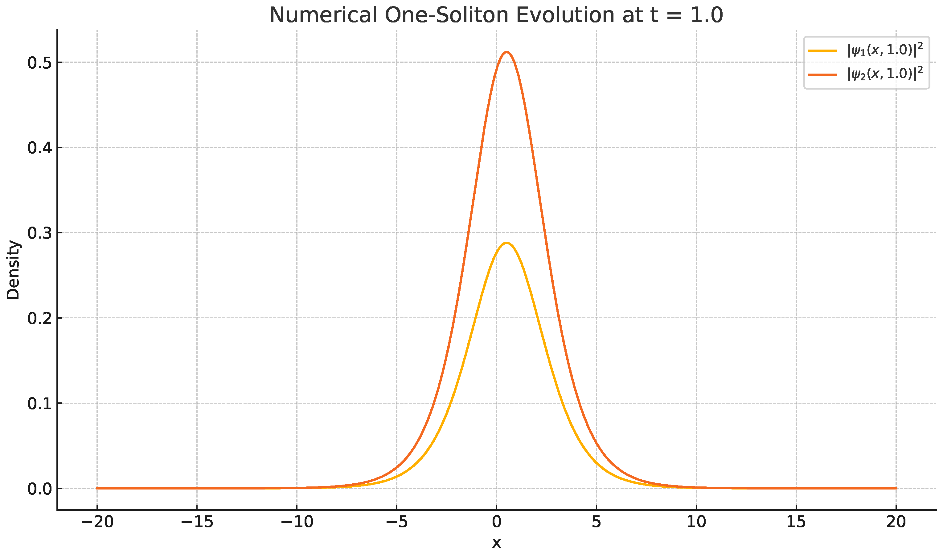
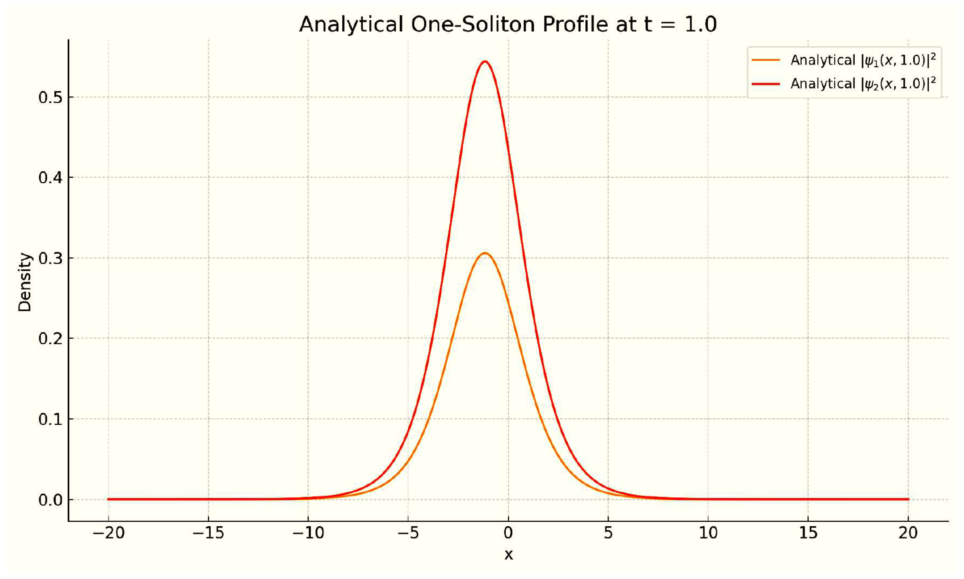
4.1. The One-Soliton Solution

Thus, the explicit form of the one-soliton solution can be written as

$$\begin{array}{ccc}\hfill {\psi }_1^{\left(1\right)}& =& \sqrt{{\displaystyle \frac{2}{\alpha \left(t\right)}}}{\epsilon }_1^{\left(1\right)}{\zeta }_{12}\left(t\right)\mathrm{sech}\left({\theta }_1\right)exp\left(\mathrm{i}(-{\xi }_1+\Gamma \left(\mathrm{t}\right){\displaystyle \frac{{\mathrm{x}}^2}{2}})\right),\hfill \end{array}$$

(27)

$$\begin{array}{ccc}\hfill {\psi }_2^{\left(1\right)}& =& \sqrt{{\displaystyle \frac{2}{\beta \left(t\right)}}}{\epsilon }_2^{\left(1\right)}{\zeta }_{12}\left(t\right)\mathrm{sech}\left({\theta }_1\right)exp\left(\mathrm{i}(-{\xi }_1+\Gamma \left(\mathrm{t}\right){\displaystyle \frac{{\mathrm{x}}^2}{2}})\right),\hfill \end{array}$$

(28)

where $\alpha \left(t\right)$ and $\beta \left(t\right)$ are time-dependent interaction coefficients, and ${\epsilon }_{1,2}$ are coupling parameters that should satisfy $|{\epsilon }_1^{\left(1\right)}{|}^2+{|{\epsilon }_2^{\left(1\right)}|}^2$ = 1. To verify the analytical solution, we performed numerical simulations using the split-step Fourier method (SSFM). Figure 1 confirms that the numerical simulations are in good agreement with the analytical solution. Minor deviations in the soliton peak positions originate from the numerical discretization and boundary conditions, which do not qualitatively affect the observed dynamics. Next, we extend our analytical approach to construct explicit two-, three-, and four-soliton solutions.

4.2. The Two-Soliton Solution

The gauge-transformation method can be easily extended to generate multi-soliton solutions. In particular, the two-component two-soliton solution ${\psi }_{1,2}^{\left(2\right)}$ can be expressed as

$$\begin{array}{ccc}\hfill {\psi }_1^{\left(2\right)}& =& {\psi }_1^{\left(1\right)}-2i({\zeta }_2-\overline{{\zeta }_2}){\tilde{P}}_{12}{\displaystyle \frac{1}{\sqrt{\alpha \left(t\right)}}}exp\left(\mathrm{i}\Gamma {\left(\mathrm{t}\right)\mathrm{x}}^2/2\right),\hfill \end{array}$$

(29)

$$\begin{array}{ccc}\hfill {\psi }_2^{\left(2\right)}& =& {\psi }_2^{\left(1\right)}-2i({\zeta }_2-\overline{{\zeta }_2}){\tilde{P}}_{13}{\displaystyle \frac{1}{\sqrt{\beta \left(t\right)}}}exp\left(\mathrm{i}\Gamma {\left(\mathrm{t}\right)\mathrm{x}}^2/2\right),\hfill \end{array}$$

(30)

where ${\zeta }_2={\overline{{\zeta }_2}}^{*}={\zeta }_{21}+i{\zeta }_{22}$, with ${\zeta }_{21}\left(t\right)={\zeta }_{210}exp(-2\int \Gamma \left(t\right)dt)$, ${\zeta }_{22}\left(t\right)$= ${\zeta }_{220}exp(-2\int \Gamma \left(t\right)dt)$ while ${\tilde{P}}_{12}$ and ${\tilde{P}}_{13}$ are elements of the projection matrix derived from matrix

$$M^{\left(2\right)}={\mathsf{\Phi }}^{\left(0\right)}(x,t,{\overline{\zeta }}_2)·\left(\begin{array}{ccc}{e}^{2{\delta }_2}\sqrt{2}& {\epsilon }_1^{\left(2\right)}{e}^{2i{\chi }_2}& {\epsilon }_2^{\left(2\right)}{e}^{2i{\chi }_2}\\ {\epsilon }_1^{*\left(2\right)}{e}^{-2i{\chi }_2}& e^{-2{\delta }_2}/\sqrt{2}& 0\\ {\epsilon }_2^{*\left(2\right)}{e}^{-2i{\chi }_2}& 0& e^{-2{\delta }_2}/\sqrt{2}\end{array}\right)·{\mathsf{\Phi }}^{\left(0\right)}{(x,t,{\zeta }_2)}^{-1}.$$

(31)

Thus, the explicit form of the two-soliton solution can be written as

$${\psi }_1^{\left(2\right)}={\displaystyle \frac{2\sqrt{2}}{\sqrt{\alpha \left(t\right)}}}{e}^{-2\int \Gamma \left(t\right)dt+{\displaystyle \frac{1}{2}}i{x}^2\Gamma \left(t\right)}\left(-{\displaystyle \frac{e^{2{\delta }_1+2i{\chi }_1}{\epsilon }_1^{\left(1\right)}{\zeta }_{20}}{D_1}}-{\displaystyle \frac{e^{2{\delta }_2+2i{\chi }_2}{\epsilon }_2^{\left(1\right)}{\zeta }_{220}}{D_2}}\right),$$

(32)

$${\psi }_2^{\left(2\right)}={\displaystyle \frac{2\sqrt{2}}{\sqrt{\beta \left(t\right)}}}{e}^{-2\int \Gamma \left(t\right)dt+{\displaystyle \frac{1}{2}}i{x}^2\Gamma \left(t\right)}\left(-{\displaystyle \frac{e^{2{\delta }_1+2i{\chi }_1}{\epsilon }_2^{\left(1\right)}{\zeta }_{20}}{D_1}}-{\displaystyle \frac{e^{2{\delta }_2+2i{\chi }_2}{\epsilon }_2^{\left(2\right)}{\zeta }_{220}}{D_2}}\right),$$

(33)

where the denominators are

$$D_1=exp\left(4{\delta }_1+4i\left[{\displaystyle \frac{1}{2}}{e}^{-2\int \Gamma \left(t\right)dt}x+\int e^{-4\int \Gamma \left(t\right)dt}dt({\zeta }_{10}+i{\zeta }_{20})\right]\left({\zeta }_{10}+i{\zeta }_{20}\right)\right)+e^{4i{\theta }_1},$$

$$D_2=exp\left(4{\delta }_2+4i\left[{\displaystyle \frac{1}{2}}{e}^{-2\int \Gamma \left(t\right)dt}x+\int e^{-4\int \Gamma \left(t\right)dt}dt({\zeta }_{210}+i{\zeta }_{220})\right]\left({\zeta }_{210}+i{\zeta }_{220}\right)\right)+e^{4i{\theta }_2},$$

and

$${\theta }_1=\int e^{-4\int \Gamma \left(t\right)dt}dt{\left({\zeta }_{10}-i{\zeta }_{20}\right)}^2+2e^{-2\int \Gamma \left(t\right)dt}x\left(i{\zeta }_{10}+{\zeta }_{20}\right),$$

$${\theta }_2=\int e^{-4\int \Gamma \left(t\right)dt}dt{\left({\zeta }_{210}-i{\zeta }_{220}\right)}^2+2e^{-2\int \Gamma \left(t\right)dt}x\left(i{\zeta }_{210}+{\zeta }_{220}\right).$$

4.3. The Three-Soliton Solution

The three-soliton solution ${\psi }_{1,2}^{\left(3\right)}$ is constructed by applying the gauge transformation a third time on the two-soliton solution ${\psi }_{1,2}^{\left(2\right)}$, resulting in:

$$\begin{array}{ccc}\hfill {\psi }_1^{\left(3\right)}& =& {\psi }_1^{\left(2\right)}-2i({\zeta }_3-{\overline{\zeta }}_3){\widehat{P}}_{12}{\displaystyle \frac{1}{\sqrt{\alpha \left(t\right)}}}exp\left(i\Gamma \left(t\right){\displaystyle \frac{x^2}{2}}\right),\hfill \end{array}$$

(34)

$$\begin{array}{ccc}\hfill {\psi }_2^{\left(3\right)}& =& {\psi }_2^{\left(2\right)}-2i({\zeta }_3-{\overline{\zeta }}_3){\widehat{P}}_{13}{\displaystyle \frac{1}{\sqrt{\beta \left(t\right)}}}exp\left(i\Gamma \left(t\right){\displaystyle \frac{x^2}{2}}\right),\hfill \end{array}$$

(35)

where ${\zeta }_3={\overline{\zeta }}_3^{*}={\zeta }_{31}+i{\zeta }_{32}$, and

$${\zeta }_{31}\left(t\right)={\zeta }_{310}exp\left(-2\int \Gamma \left(t\right)dt\right),{\zeta }_{32}(t)={\zeta }_{320}exp\left(-2\int \Gamma (t)dt\right).$$

The projection matrix elements ${\widehat{P}}_{12}$ and ${\widehat{P}}_{13}$ are derived from matrix $M^{\left(3\right)}$ as:

$$M^{\left(3\right)}={\mathsf{\Phi }}^{\left(0\right)}(x,t,{\overline{\zeta }}_3)·\left(\begin{array}{ccc}{e}^{2{\delta }_3}\sqrt{2}& {\epsilon }_1^{\left(3\right)}{e}^{2i{\chi }_3}& {\epsilon }_2^{\left(3\right)}{e}^{2i{\chi }_3}\\ {\epsilon }_1^{*\left(3\right)}{e}^{-2i{\chi }_3}& {\displaystyle \frac{e^{-2{\delta }_3}}{\sqrt{2}}}& 0\\ {\epsilon }_2^{*\left(3\right)}{e}^{-2i{\chi }_3}& 0& {\displaystyle \frac{e^{-2{\delta }_3}}{\sqrt{2}}}\end{array}\right)·{\mathsf{\Phi }}^{\left(0\right)}{(x,t,{\zeta }_3)}^{-1}.$$

Thus, the three-soliton state takes the following general form

$${\psi }_{1,2}^{\left(3\right)}(x,t)={\displaystyle \frac{2\sqrt{2}{e}^{-2I+\frac{1}{2}i{x}^2\Gamma \left(t\right)}}{\sqrt{\pm \alpha \left(t\right)}}}\sum _{j=1}^3-{\displaystyle \frac{{\zeta }_{j0}{\epsilon }_{j1}{e}^{2{\delta }_j+2i{\chi }_j}}{D_{3j}(x,t)}}$$

(36)

and the denominator $D_{3j}(x,t)$ is

$$\begin{array}{c}\hfill D_{3j}(x,t)=exp\left(4{\delta }_j+4i({\zeta }_{j0}+i{\zeta }_{j20})\left({\displaystyle \frac{1}{2}}x{e}^{-2I}+({\zeta }_{j0}+i{\zeta }_{j20})J\right)\right)\\ \hfill +exp\left(4i{({\zeta }_{j0}-i{\zeta }_{j20})}^{2}J+2({\zeta }_{j20}+i{\zeta }_{j0})x{e}^{-2I}\right)\end{array}$$

where $J=\int e^{-4I}dt$, $I=\int \Gamma \left(t\right)dt$. Here, the ± in the denominator corresponds to $+\alpha \left(t\right)$ for ${\psi }_1^{\left(3\right)}$ and $-\alpha \left(t\right)=\beta \left(t\right)$ for ${\psi }_2^{\left(3\right)}$.

4.4. The Four-Soliton Solution

By applying the gauge transformation a fourth time, the four-soliton solution ${\psi }_{1,2}^{\left(4\right)}$ is obtained:

$$\begin{array}{ccc}\hfill {\psi }_1^{\left(4\right)}& =& {\psi }_1^{\left(3\right)}-2i({\zeta }_4-{\overline{\zeta }}_4){\overline{P}}_{12}{\displaystyle \frac{1}{\sqrt{\alpha \left(t\right)}}}exp\left(i\Gamma \left(t\right){\displaystyle \frac{x^2}{2}}\right),\hfill \end{array}$$

(37)

$$\begin{array}{ccc}\hfill {\psi }_2^{\left(4\right)}& =& {\psi }_2^{\left(3\right)}-2i({\zeta }_4-{\overline{\zeta }}_4){\overline{P}}_{13}{\displaystyle \frac{1}{\sqrt{\beta \left(t\right)}}}exp\left(i\Gamma \left(t\right){\displaystyle \frac{x^2}{2}}\right),\hfill \end{array}$$

(38)

where ${\zeta }_4={\overline{\zeta }}_4^{*}={\zeta }_{41}+i{\zeta }_{42}$, and

$${\zeta }_{41}\left(t\right)={\zeta }_{410}exp\left(-2\int \Gamma \left(t\right)dt\right),{\zeta }_{42}(t)={\zeta }_{420}exp\left(-2\int \Gamma (t)dt\right).$$

The projection matrix for the fourth soliton is derived from matrix $M^{\left(4\right)}$ as:

$$M^{\left(4\right)}={\mathsf{\Phi }}^{\left(0\right)}(x,t,{\overline{\zeta }}_4)·\left(\begin{array}{ccc}{e}^{2{\delta }_4}\sqrt{2}& {\epsilon }_1^{\left(4\right)}{e}^{2i{\chi }_4}& {\epsilon }_2^{\left(4\right)}{e}^{2i{\chi }_4}\\ {\epsilon }_1^{*\left(4\right)}{e}^{-2i{\chi }_4}& {\displaystyle \frac{e^{-2{\delta }_4}}{\sqrt{2}}}& 0\\ {\epsilon }_2^{*\left(4\right)}{e}^{-2i{\chi }_4}& 0& {\displaystyle \frac{e^{-2{\delta }_4}}{\sqrt{2}}}\end{array}\right)·{\mathsf{\Phi }}^{\left(0\right)}{(x,t,{\zeta }_4)}^{-1}.$$

The explicit form of the four-soliton solution is

$${\psi }_{1,2}^{\left(4\right)}(x,t)={\displaystyle \frac{2\sqrt{2}{e}^{-2I+\frac{1}{2}i{x}^2\Gamma \left(t\right)}}{\sqrt{\pm \alpha \left(t\right)}}}\sum _{j=1}^4-{\displaystyle \frac{{\zeta }_{j0}{\epsilon }_{j1}{e}^{2{\delta }_j+2i{\chi }_j}}{D_{4j}(x,t)}},$$

(39)

where $I=\int \Gamma \left(t\right)dt$, $J=\int e^{-4I}dt$, and the denominator $D_{4j}(x,t)$ is

$$\begin{array}{c}\hfill D_{4j}(x,t)=exp\left(4{\delta }_j+2i({\zeta }_{j0}+i{\zeta }_{j20})e^{-2I}\left(x+2({\zeta }_{j0}+i{\zeta }_{j20})e^{2I}J\right)\right)\\ \hfill +exp\left(2({\zeta }_{j0}-i{\zeta }_{j20})e^{-2I}\left(2({\zeta }_{j20}+i{\zeta }_{j0})e^{2I}J+ix\right)\right).\end{array}$$

(40)

Note that the constraint $|{\epsilon }_1^{\left(j\right)}{|}^2+{|{\epsilon }_2^{\left(j\right)}|}^2=1$ for $j=1,2,3,4$ applies to the coupling parameters used in constructing the multi-soliton solution. These parameters determine the internal distribution of amplitude between the two components in each soliton. This relation does not impose a direct constraint on the physical condensate densities $|{\psi }_1{(x,t)|}^2$ and $|{\psi }_2{(x,t)|}^2$, which evolve according to the full analytical solution.

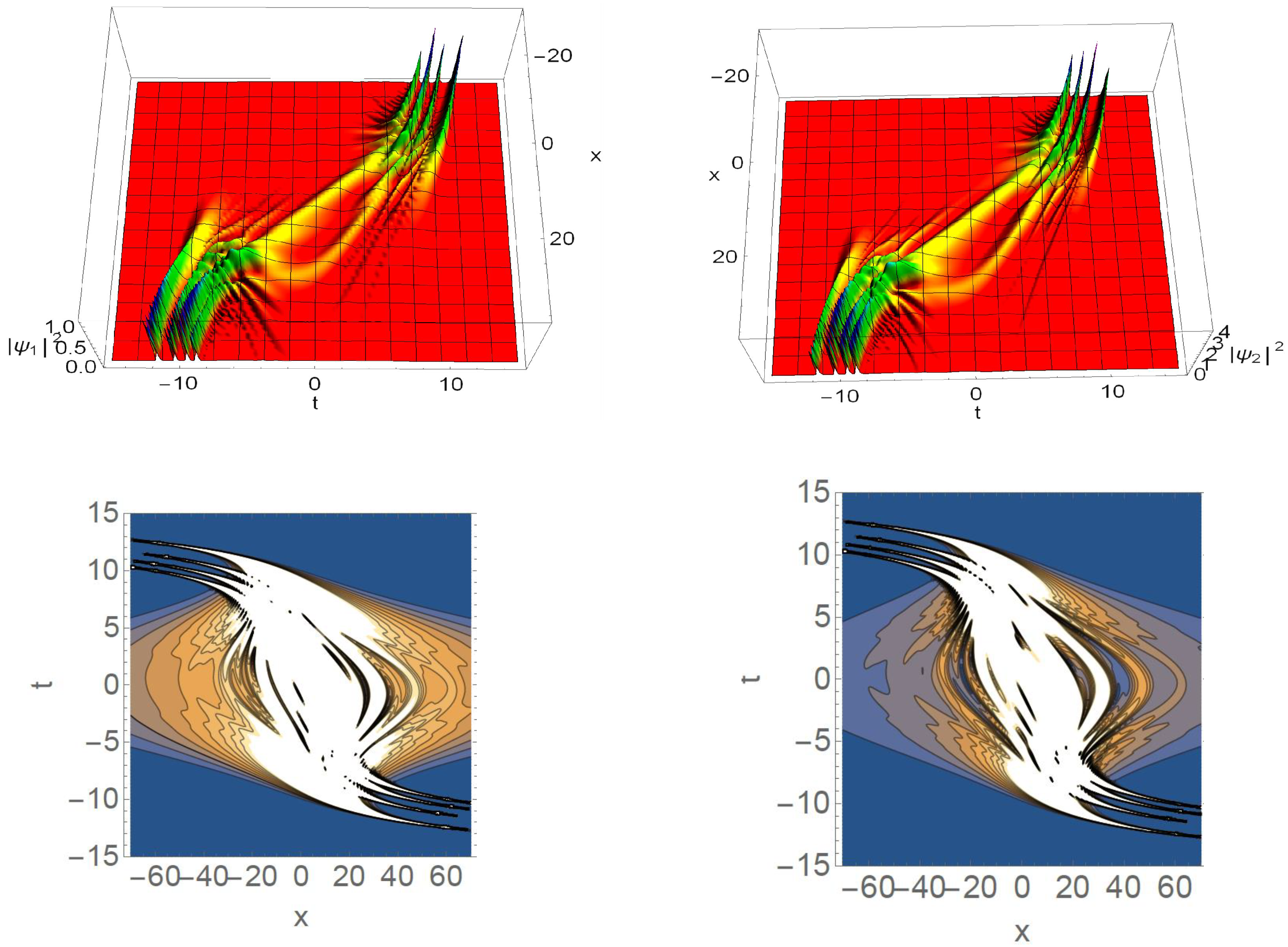
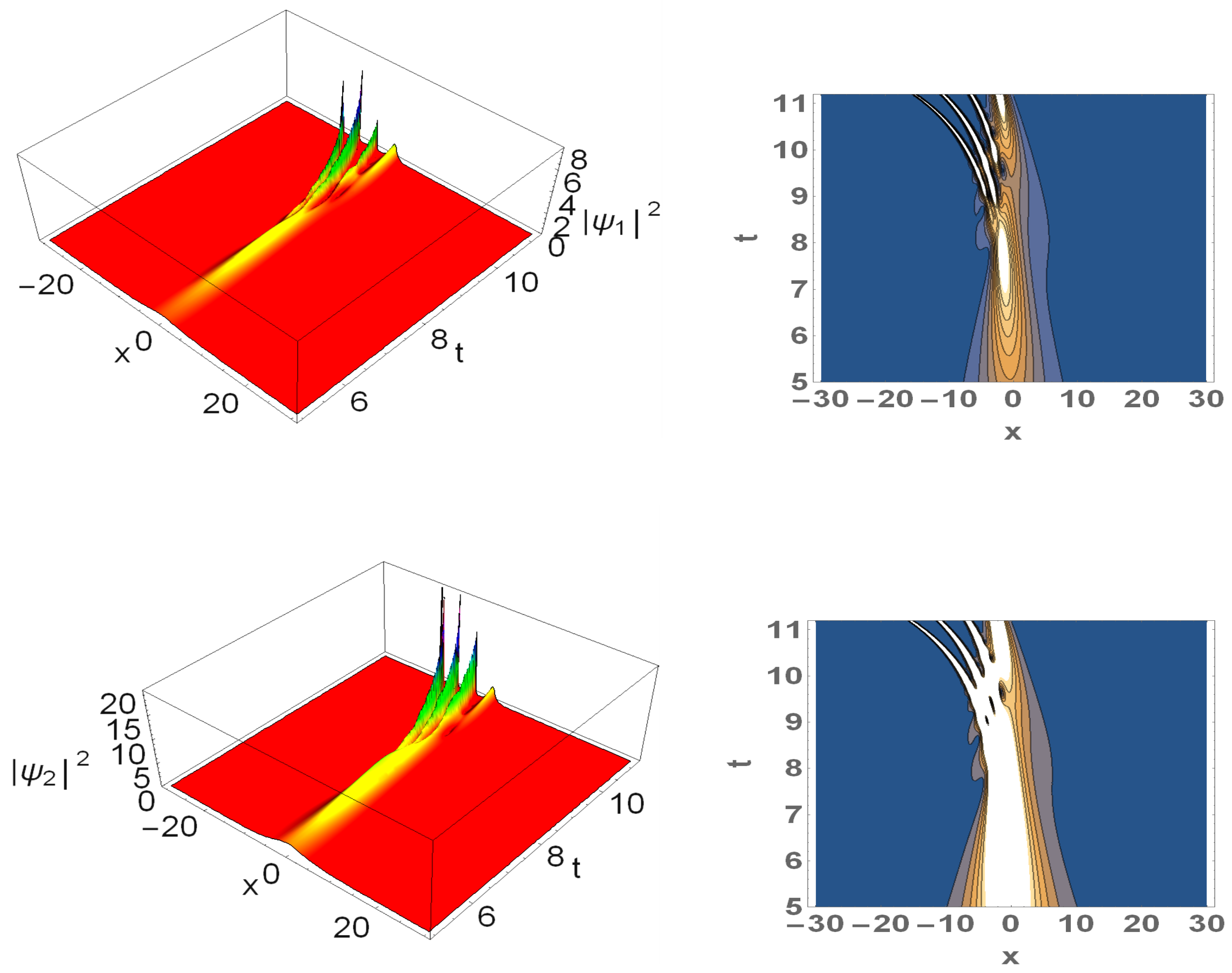
5. Dynamics of the Four-Soliton Solution

5.1. General Consideration

The solution given in Equation (39) demonstrates that the amplitude of ${\psi }_{1,2}^{\left(4\right)}(x,t)$ is mainly affected by the exponential prefactor $e^{-2I}$, which depends on $\Gamma \left(t\right)$ via $I=\int \Gamma \left(t\right)dt$. This term can introduce growth, decay, or oscillations. The denominator $D_{4j}(x,t)$ governs the location and interactions of the soliton. If $\Gamma \left(t\right)$ varies in time, the overall amplitude of ${\psi }_{1,2}^{\left(4\right)}(x,t)$ changes too. If $\Gamma \left(t\right)$ is constant, the soliton’s amplitudes may only change due to interactions.

The peak location of the solitons can be determined as $x_j^{\mathrm{peak}}\left(t\right)\approx -2({\zeta }_{j0}+i{\zeta }_{j20})e^{2I}J$. Because $J=\int e^{-4I}dt$, the position of the soliton’s maximum depends on the integral of $e^{-4I}$. The velocity is obtained by $v_j\left(t\right)=d{x}_j^{\mathrm{peak}}/dt$. The time-dependent factor $e^{2I}$ means that the soliton may accelerate or decelerate, depending on $\Gamma \left(t\right)$. The soliton’s phase is $\varphi (x,t)=-2I+{\displaystyle \frac{1}{2}}{x}^2\Gamma \left(t\right)+{\sum }_{j=1}^4(2{\chi }_j-arg\left(D_{4j}(x,t)\right)$. The first term, $-2I$, evolves with $\Gamma \left(t\right),$ introducing a global phase shift. The quadratic term ${\displaystyle \frac{1}{2}}{x}^2\Gamma \left(t\right)$ suggests that $\Gamma \left(t\right)$ contributes to the quadratic chirp, modifying the wavefront curvature. The argument of $D_{4j}(x,t)$ affects phase shifts produced by interactions between solitons.

We can now suitably tune the trapping frequency ${\lambda }^2\left(t\right)={\Gamma }^2\left(t\right)+{\Gamma }^{\prime }\left(t\right)/2$ and the intra-/intercomponent interaction coefficients $\alpha \left(t\right)$ to reveal the nonlinear excitations. The polarization coefficients, such as ${\epsilon }_1^{\left(1\right)}$ and its counterparts, determine the population balance between soliton states. These coefficients can be interpreted as probability amplitudes in the two-component BEC, which represent quantum states in the qubit basis [35]. Specifically, the state of the soliton can be written as $|\psi \rangle ={\epsilon }_1^{\left(1\right)}|1\rangle +{\epsilon }_2^{\left(1\right)}|0\rangle$, demonstrating a direct similarity to the qubit representation. By carefully tuning the polarization parameters, it is possible to manipulate the quantum state of the system. Hence, this framework offers a classical counterpart of the qubit-like behavior, which may be useful for simulating the basic quantum logic [35,36,37,38]. The parameters ${\zeta }_{i0}$, ${\delta }_i$, and $\Gamma \left(t\right)$ play a crucial role in determining how solitons separate and interact over time. The expression for the velocity, $v_i=-2{\zeta }_{i0}exp\left(-2\int \Gamma \left(t\right)dt\right)$, suggests that adjusting ${\zeta }_{i0}$ or the time-dependent function $\Gamma \left(t\right)$ can effectively control the speed at which solitons move apart, affecting the fission rate. Meanwhile, amplitude $A_i=2\sqrt{2}{\zeta }_{i0}{e}^{2{\delta }_i}$ determines the energy distribution between the emerging solitons, meaning that varying ${\delta }_i$ can control post-fission intensity variations. By fine-tuning these parameters, it is possible to modulate soliton interactions, delay, or accelerate the fission, and even regulate energy transfer between solitonic components.

5.2. Superposition States of Four Solitons

Figure 2 illustrates the superposition dynamics of the four-soliton state in a two-component BEC. The top panel shows the individual density distributions of both components $|{\psi }_1{(x,t)|}^2$ and $|{\psi }_2{(x,t)|}^2$ of Equation (39), where the interference patterns and energy sharing between solitons in each component are evident. The bottom panel presents a contour plot of the superposition state visualizing the evolving structure of the four-soliton interaction. The periodic modulation of the interaction strength, $\alpha \left(t\right)=0.1cos\left(0.02t\right)$, stabilizes the soliton dynamics, while the linear phase shift function, $\Gamma \left(t\right)=-0.03t$, contributes to global temporal phase modulation. The real parts of the complex spectral parameters, which determine the soliton velocities, were chosen as ${\zeta }_{10}=0.2$, ${\zeta }_{20}=0.01$, ${\zeta }_{210}=0.4$, ${\zeta }_{220}=0.04$, ${\zeta }_{310}=0.6$, ${\zeta }_{320}=0.06$, ${\zeta }_{410}=0.8$, and ${\zeta }_{420}=0.08$. These values set distinct group velocities and allowed for an observable superposition during propagation. The amplitude scaling factors ${\delta }_1=0.1$, ${\delta }_2=0.4$, ${\delta }_3=0.6$, and ${\delta }_4=0.08$ controlled the energy and peak height of each soliton. Phase offsets between the components were tuned using ${\chi }_1=0.01$, ${\chi }_2=0.03$, ${\chi }_3=0.05$, and ${\chi }_4=0.7$. During the central interval, the solitons exhibited coherent overlap and interference, resembling quantum superposition. Outside this regime, the solitons separated, analogously modeling quantum decoherence where entangled states collapse into distinguishable ones. This dynamic demonstrates the potential for simulating quantum logic operations within classical nonlinear systems [28,35,36,37,38].

5.3. Controlled Fission of Four-Soliton States

Figure 3 illustrates the controlled fission of a four-soliton state of a two-component BEC. The density and contour plots show that the solitons are initially bound and gradually separate over time due to the influence of time-dependent system parameters. The intra- and interspecies interaction coefficients, modulated by $\alpha \left(t\right)=0.1cos\left(0.002t\right)$, regulate the soliton interactions and ensure a well-controlled fission process. The external potential, defined by the phase function $\Gamma \left(t\right)=-0.035t$, introduces a linear time-dependent phase shift that alters the trajectories of the soliton peaks. The real parts of the complex spectral parameters, selected as ${\zeta }_{10}=0.01$, ${\zeta }_{20}=0.01$, ${\zeta }_{210}=0.03$, ${\zeta }_{220}=0.04$, ${\zeta }_{310}=0.05$, ${\zeta }_{320}=0.06$, ${\zeta }_{410}=0.07$, and ${\zeta }_{420}=0.08$, define the soliton velocities and result in slightly separated propagation paths. The amplitude parameters ${\delta }_1=0.01$, ${\delta }_2=0.04$, ${\delta }_3=0.06$, and ${\delta }_4=0.08$ control the initial pulse strengths and energy content of each soliton. Phase constants ${\chi }_1=0.01$, ${\chi }_2=0.03$, ${\chi }_3=0.05$, and ${\chi }_4=0.07$ regulate the initial internal phase shifts of each component. The polarization coefficients ${\epsilon }_1^{\left(1\right)}=0.4$, ${\epsilon }_1^{\left(2\right)}=0.2$, ${\epsilon }_1^{\left(3\right)}=0.3$, and ${\epsilon }_1^{\left(4\right)}=0.2$ determine the population imbalance between the two components of the system and enabled distinct soliton identities. The evolution of the peak positions, governed by the relation

$$x_j\left(t\right)=-2{\zeta }_{j0}exp\left(-2\int \Gamma (t)dt\right)J\left(t\right),$$

shows that each soliton moves away from the origin gradually, indicating controlled spatial separation. Throughout this process, the soliton amplitudes remain approximately constant in time, demonstrating the preservation of localized energy and coherence, even as the solitons dynamically redistribute in space. This controllable fission mechanism may find direct applications in quantum information processing, where soliton states can be manipulated similar to qubits in quantum computing. Recent studies have demonstrated the potential of soliton-based qubit states for metrological applications, highlighting the versatility of the soliton dynamics in quantum technologies [38].

Figure 4 presents a symmetric four-soliton fission process, where the solitons separate evenly in both positive and negative x-directions. Unlike the asymmetric propagation in Figure 3, this case was achieved by choosing symmetric initial soliton parameters (e.g., ${\zeta }_{10}=-0.01$, ${\zeta }_{20}=0.01$, ${\zeta }_{30}=-0.05$, ${\zeta }_{40}=0.07$). The periodic modulation of the interaction strength, viz., $\alpha \left(t\right)=0.1cos\left(0.2t\right)$, introduces oscillatory behavior that affects the soliton-separation dynamics. The phase function $\Gamma \left(t\right)=-0.035t$ further modulates the relative phase differences, impacting the symmetry of the fission. This symmetric splitting is significant for applications in nonlinear optics and matter-wave engineering, where stability and coherence are crucially important for robust wave propagation. Additionally, the symmetric fission provides a physical analogy to controlled quantum-gate operations, where entangled soliton components evolve into separate, distinguishable quantum states, highlighting the potential of using the two-component solitons for quantum information applications. Recent experimental and theoretical studies have revealed soliton complexes composed of multiple solitons in close spatial proximity, resulting in frequent and strong interactions within two-component BECs. These dense configurations offer important insights into the dynamics of multi-soliton collisions and collective behavior [39].

5.4. Elastic Collision of Four-Soliton States

Figure 5 depicts the elastic collision of a four-soliton state in the two-component BEC under the action of the time-dependent potential. The solitons interact and emerge with their initial shape and velocity preserved, confirming the integrability of the system. The soliton dynamics are affected by the time-dependent scattering length $\alpha \left(t\right)=0.1e^{0.02t}$, which gradually modulates the interaction strength, securing the stable evolution. Additionally, the weak phase shift introduced by $\Gamma \left(t\right)=-0.002t$ contributes to minor trajectory variations without disrupting the coherence. The initial parameters were chosen to generate four distinct soliton pulses, ${\delta }_1=0.75$, ${\delta }_2=0.82$, ${\delta }_3=0.69$, and ${\delta }_4=0.85$, to control the amplitude scaling of each soliton. The velocity parameters were ${\zeta }_{10}=0.1$, ${\zeta }_{20}=0.2$, ${\zeta }_{210}=0.3$, ${\zeta }_{220}=0.4$, ${\zeta }_{310}=0.5$, ${\zeta }_{320}=0.6$, ${\zeta }_{410}=0.7$, and ${\zeta }_{420}=0.8$, which determined the propagation speed of each soliton. The relative phase parameters were set to ${\chi }_1=0.9$, ${\chi }_2=0.75$, ${\chi }_3=0.8$, and ${\chi }_4=0.9$. The polarization coefficients ${\epsilon }_1^{\left(1\right)}=0.6$, ${\epsilon }_1^{\left(2\right)}=0.5$, ${\epsilon }_1^{\left(3\right)}=0.4$, and ${\epsilon }_1^{\left(4\right)}=0.7$ determined the population distribution across the two components. The external modulation was given by a weakly time-dependent trap $\Gamma \left(t\right)=-0.002t$ and nonlinear coefficient $\alpha \left(t\right)=0.1exp\left(0.02t\right)$. The figure demonstrates that the solitons undergo elastic interactions; they pass through each other without distortion, and their shapes and velocities are preserved after collision. The elastic nature of the collision, in which the solitons retain their identity post-interaction, contrasts with inelastic processes that lead to fusion or decay. This soliton-collision mode may have significant implications in nonlinear optics and quantum information, where soliton-like wave packets can act as robust carriers of quantum information, undergoing coherent transformations without loss of integrity.

All analytical figures were plotted using the exact four-soliton solution Equation (39) derived in Section 4. Figure 1 was generated using the split-step Fourier method applied to Equations (3) and (4) with the time-dependent coefficients. An important feature of this system is its ability to maintain coherence through controlled oscillations of $\alpha \left(t\right)$. This feature prevents the onset of decoherence, which is a major challenge in quantum computing. The ability to fine-tune soliton interactions via velocity and position parameters allows one to maintain precise control over quantum-gate operations, ensuring robust and fault-tolerant quantum computations. Compared to earlier studies on two-soliton interactions [29], the current four-soliton setting exhibits higher-order collective behavior such as simultaneous fission and elastic scattering. Unlike the binary soliton logic suggested in [38], our approach enables more complex superposition-controlled fission and symmetric energy splitting, as illustrated in Figure 2, Figure 3 and Figure 4. These processes are facilitated by the extra degrees of freedom introduced by additional spectral parameters ${\zeta }_{j0}$, amplitude controls ${\delta }_j$, and polarization coefficients ${\epsilon }_j$. The ability to tune these parameters independently allows fine-tuned control over the soliton trajectories, phase evolution, and population distribution between the components. This makes the four-soliton setting a promising platform for simulating more complex quantum-like dynamics.

Thus, the controlled fission of the solitons in the two-component BEC has profound implications for qubit control in quantum computing. In that context, qubits are fundamental data units, capable of existing in superpositions of states. Matter-wave solitons in a BEC can represent localized quantum states, due to their stability and coherence, making them potential candidates for qubit encoding and manipulations. The controlled fission of solitons, when a multi-soliton state splits into separate solitons, is similar to the quantum-gate operation, in which an entangled qubit system undergoes a controlled separation or interaction. This extension from two- to four-soliton states enriches the soliton-based qubit modeling, previously addressed in [38], by enabling enhanced state encoding via the polarization and velocity control. We stress that the displayed figures represent typical dynamical behaviors of multi-soliton states under a broad range of parameter choices. While specific values were selected to highlight key features, such as controlled fission, superposition, and elastic collisions, these outcomes are robust, persisting across variations in soliton amplitudes, phases, and interaction coefficients, and thus indicating that the results reflect generic situations in the framework of the integrable model. We note that the model’s integrability is predicated on the constraints pertaining to the intra- and interatomic interactions in the presence of the external trapping potential, and that gain is hard to implement in practical BEC experiments. Nevertheless, integrable models can be used as accurate approximations for finite-time evolution or under strict experimental control, offering valuable insight into the picture of soliton interactions.

The key parameters governing the soliton dynamics in the present context are summarized as follows: ${\zeta }_{j0}$ controls the velocity of the jth soliton, and ${\delta }_j$ determines the amplitude and energy distribution. Parameter ${\chi }_j$ represents the relative phase between the solitons, and ${\epsilon }_j$ describes the population distribution between the two components, similar to coefficients of a qubit state. The time-dependent trap parameter $\Gamma \left(t\right)$ affects the soliton’s chirp, spatial separation, and effective phase evolution. In Figure 2, Figure 3 and Figure 4, parameters such as ${\zeta }_{j0}$ determine the soliton’s velocity via relation $v_j=-2{\zeta }_{j0}exp\left(-2\int \Gamma \left(t\right)dt\right)$, while ${\delta }_j$ controls the amplitude scaling factor. The choice of these parameters directly affects the separation degree, overlap, and interference between the solitons.

6. Conclusions

In this work, the dynamics of vector solitons in the two-component BEC (Bose–Einstein condensate) governed by coupled Gross–Pitaevskii equations were systematically investigated. Explicit multi-soliton solutions, including two-, three-, and four-soliton states, were derived using the gauge-transformation method. We highlighted the effect of the time-dependent intra- and intercomponent interaction coefficients and external potential on the soliton’s amplitude and its evolution. The controlled four-soliton fission was demonstrated, showing the ability to manipulate the soliton separation and interaction by means of the external parameters. We also identified elastic four-solitons collisions, with the solitons retaining their identity post-interaction. These findings underscore the potential of the two-component solitons for applications in coherent matter-wave transport, nonlinear optics, and quantum information processing, in particular, for modeling qubit states and gate operations. Future research may uphold experimental realizations of these soliton states and their use in quantum technologies.

References

1. Bose, S.N. Plancks Gesetz und Lichtquantenhypothese. Z. Phys. 1924, 26, 178. [Google Scholar] [CrossRef]
2. Einstein, A. Quantentheorie des einatomigen idealen Gases. Sitzber. Kgl. Preuss. Akad. Wiss. 1924, 22, 261. [Google Scholar]
3. Anderson, M.H.; Ensher, J.R.; Matthews, M.R.; Wieman, C.E.; Cornell, E.A. Observation of Bose-Einstein condensation in a dilute atomic vapor. Science 1995, 269, 198. [Google Scholar] [CrossRef] [PubMed]
4. Davis, K.B.; Mewes, M.-O.; Andrews, M.R.; van Druten, N.J.; Durfee, D.S.; Kurn, D.M.; Ketterle, W. Bose-Einstein Condensation in a Gas of Sodium Atoms. Phys. Rev. Lett. 1995, 75, 3969. [Google Scholar] [CrossRef] [PubMed]
5. Bradley, C.C.; Sackett, C.A.; Tollett, J.J.; Hulet, R.G. Evidence of Bose-Einstein condensation in an atomic gas with attractive interactions. Phys. Rev. Lett. 1995, 75, 1687–1690, Erratum in Phys. Rev. Lett. 1997, 79, 1170. [Google Scholar] [CrossRef] [PubMed]
6. Strecker, K.E.; Partridge, G.B.; Truscott, A.G.; Hulet, R.G. Formation and propagation of matter-wave soliton trains. Nature 2002, 417, 150. [Google Scholar] [CrossRef] [PubMed]
7. Khaykovich, L.; Schreck, F.; Ferrari, G.; Bourdel, T.; Cubizolles, J.; Carr, L.D.; Castin, Y.; Salomon, C. Formation of a matter-wave bright soliton. Science 2002, 296, 1290. [Google Scholar] [CrossRef] [PubMed]
8. Burger, S.; Bongs, K.; Dettmer, S.; Ertmer, W.; Sengstock, K.; Sanpera, A.; Shlyapnikov, G.V.; Lewenstein, M. Dark solitons in Bose–Einstein condensates. Phys. Rev. Lett. 1999, 83, 5198. [Google Scholar] [CrossRef]
9. Frantzeskakis, D.J. Dark solitons in atomic Bose–Einstein condensates: From theory to experiments. J. Phys. A Math. Theor. 2010, 43, 213001. [Google Scholar] [CrossRef]
10. Theocharis, G.; Frantzeskakis, D.J.; Kevrekidis, P.G.; Malomed, B.A.; Kivshar, Y.S. Ring dark solitons and vortex necklaces in Bose–Einstein condensates. Phys. Rev. Lett. 2003, 90, 120403. [Google Scholar] [CrossRef] [PubMed]
11. Liang, Z.X.; Zhong, Z.D.; Liu, W.M. Dynamical generation of bright solitons in a quasi-one-dimensional condensate. Phys. Rev. Lett. 2005, 94, 050402. [Google Scholar] [CrossRef] [PubMed]
12. Dalfovo, F.; Giorgini, S.; Pitaevskii, L.P.; Stringari, S. Theory of Bose–Einstein condensation in trapped gases. Rev. Mod. Phys. 1999, 71, 463. [Google Scholar] [CrossRef]
13. Pethick, C.J.; Smith, H. Bose–Einstein Condensation in Dilute Gases; Cambridge University Press: Cambridge, UK, 2002. [Google Scholar]
14. Ho, T.L.; Shenoy, V.B. Binary mixtures of Bose condensates of alkali atoms. Phys. Rev. Lett. 1996, 77, 3276. [Google Scholar] [CrossRef] [PubMed]
15. Kasamatsu, K.; Tsubota, M.; Ueda, M. Vortices in multicomponent Bose-Einstein condensates. Int. J. Mod. Phys. B 2005, 19, 1835. [Google Scholar] [CrossRef]
16. Kevrekidis, P.G.; Frantzeskakis, D.J.; Carretero-González, R. Emergent Nonlinear Phenomena in Bose-Einstein Condensates: Theory and Experiment; Springer: Berlin/Heidelberg, Germany, 2008. [Google Scholar]
17. Stoof, H.T.C.; Gubbels, K.B.; Dickerscheid, D.B.M. Ultracold Quantum Fields; Springer: Dordrecht, The Netherlands, 2009. [Google Scholar]
18. Ieda, J.; Miyakawa, T.; Wadati, M. Exact analysis of soliton dynamics in spinor Bose-Einstein condensates. Phys. Rev. Lett. 2004, 93, 194102. [Google Scholar] [CrossRef] [PubMed]
19. Alotaibi, M.O.D.; Carr, L.D. Dynamics of dark-bright vector solitons in Bose-Einstein condensates. Phys. Rev. A 2017, 96, 013601. [Google Scholar] [CrossRef]
20. He, Z.-M.; Zhu, Q.-Q.; Zho, X. The controlled fission, fusion and collision behavior of two species Bose–Einstein condensates with an optical potential. Z. Naturforschung A 2023, 78, 589. [Google Scholar] [CrossRef]
21. Busch, T.; Anglin, J.R. Dark-bright solitons in inhomogeneous Bose-Einstein condensates. Phys. Rev. Lett. 2001, 87, 010401. [Google Scholar] [CrossRef] [PubMed]
22. Ohberg, P.; Santos, L. Dark Solitons in a Two-Component Bose-Einstein Condensate. Phys. Rev. Lett. 2001, 86, 2918. [Google Scholar] [CrossRef] [PubMed]
23. Kasamatsu, K.; Tsubota, M. Modulation instability and solitary-wave formation in two-component Bose-Einstein condensates. Phys. Rev. A 2006, 74, 013617. [Google Scholar] [CrossRef]
24. Dauxois, T.; Peyrard, M. Physics of Solitons; Cambridge University Press: Cambridge, UK, 2006. [Google Scholar]
25. Kivshar, Y.S.; Agrawal, G.P. Optical Solitons: From Fibers to Photonic Crystals; Academic Press: San Diego, CA, USA, 2003. [Google Scholar]
26. Porsezian, K.; Sundaram, P.S.; Mahalingam, A. Coupled higher-order nonlinear Schrödinger equations in nonlinear optics: Painlevé analysis and integrability. Phys. Rev. E 1994, 50, 1543. [Google Scholar] [CrossRef] [PubMed]
27. Radhakrishnan, R.; Lakshmanan, M. Exact soliton solutions to coupled nonlinear Schrödinger equations with higher-order effects. Phys. Rev. E 1996, 54, 2949. [Google Scholar] [CrossRef] [PubMed]
28. Kanna, T.; Lakshmanan, M. Exact soliton solutions of coupled nonlinear Schrödinger equations: Shape-changing collisions, logic gates, and partially coherent solitons. Phys. Rev. Lett. 2001, 86, 5043. [Google Scholar] [CrossRef] [PubMed]
29. Kumar, V.R.; Radha, R.; Wadati, M. Collision of bright vector solitons in two-component Bose-Einstein condensates. Phys. Lett. A 2010, 374, 3685. [Google Scholar] [CrossRef]
30. Abdullaev, F.K.; Caputo, J.G.; Kraenkel, R.A.; Malomed, B.A. Controlling collapse in Bose-Einstein condensation by temporal modulation of the scattering length. Phys. Rev. A 2003, 67, 013605. [Google Scholar] [CrossRef]
31. Saito, H.; Ueda, M. Dynamically stabilized bright solitons in a two-dimensional Bose-Einstein condensate. Phys.Rev. Lett. 2003, 90, 040403. [Google Scholar] [CrossRef] [PubMed]
32. Luo, Z.; Liu, Y.; Li, Y.; Batle, J.; Malomed, B.A. Stability limits for modes held in alternating trapping-expulsive potentials. Phys. Rev. E 2022, 106, 014201. [Google Scholar] [CrossRef] [PubMed]
33. Manakov, S.V. On the theory of two-dimensional stationary self-focusing of electromagnetic waves. Sov. Phys. JETP 1974, 38, 248. [Google Scholar]
34. Chau, L.-L.; Shaw, J.C.; Yen, H.C. An alternative explicit construction of N-soliton solutions in 1+1 dimensions. J. Math. Phys. 1991, 32, 1737–17434. [Google Scholar] [CrossRef]
35. Byrnes, T.; Wen, K.; Yamamoto, Y. Macroscopic quantum computation using Bose-Einstein condensates. Phys. Rev. A 2012, 85, 040306(R). [Google Scholar] [CrossRef]
36. Konyukhov, A. Quantum correlations via vector soliton interactions. Phys. Rev. A 2025, 111, 013508. [Google Scholar] [CrossRef]
37. Shaukat, M.I.; Castro, E.V.; Tercas, H. Quantum dark solitons as qubits in Bose–Einstein condensates. Phys. Rev. A 2017, 95, 053618. [Google Scholar] [CrossRef]
38. Ngo, T.V.; Tsarev, D.V.; Lee, R.; Alodjants, A.P. Bose–Einstein condensate soliton qubit states for metrological applications. Sci. Rep. 2021, 11, 19363. [Google Scholar] [CrossRef] [PubMed]
39. Mossman, S.M.; Katsimiga, G.C.; Mistakidis, S.I.; Romero-Ros, A.; Bersano, T.M.; Schmelcher, P.; Kevrekidis, P.G.; Engels, P. Observation of dense collisional soliton complexes in a two-component Bose-Einstein condensate. Commun. Phys. 2024, 7, 163. [Google Scholar] [CrossRef]
Figure 1. (Top panel): The numerically evolved one-soliton state at t = 1.0 for both components | ψ 1 ( x , t ) | 2 and | ψ 2 ( x , t ) | 2 . (Bottom panel): The corresponding analytical one-soliton solution evaluated at t = 1.0 . The close agreement between the analytical and numerical results confirms the accuracy of the analytical solution and the stability of the system under time-dependent coefficients. The parameters used are ε 1 ( 1 ) = 0.6 , ε 2 ( 1 ) = 0.8 such that | ε 1 ( 1 ) | 2 + | ε 2 ( 1 ) | 2 = 1 , ζ 10 = 0.4 , ζ 20 = 0.2 , δ 1 = 0.1 , and χ 1 = 0.2 . The coupling coefficients are time-dependent, α ( t ) = β ( t ) = 0.1 cos ( 0.02 t ) , and the phase modulation is given by Γ ( t ) = 0.03 t .
Symmetry 17 01189 g001aSymmetry 17 01189 g001b
Figure 2. (Top panel): Density plots of the individual components | ψ 1 ( x , t ) | 2 and | ψ 2 ( x , t ) | 2 given by Equation (39), showing the evolution and superposition state of four-soliton in a two-component Bose–Einstein condensate. (Bottom panel): The contour plot of the superposition state highlighting the coherent soliton interference. The interaction strength is modulated by α ( t ) = 0.1 cos ( 0.02 t ) , and the phase function is governed by Γ ( t ) = 0.03 t . Parameters used: δ 1 = 0.1 , δ 2 = 0.4 , δ 3 = 0.6 , δ 4 = 0.08 , ζ 10 = 0.2 , ζ 20 = 0.01 , ζ 210 = 0.4 , ζ 220 = 0.04 , ζ 310 = 0.6 , ζ 320 = 0.06 , ζ 410 = 0.8 , ζ 420 = 0.08 , χ 1 = 0.01 , χ 2 = 0.03 , χ 3 = 0.05 , χ 4 = 0.7 ; ε 1 ( 1 ) = 0.4 , ε 1 ( 2 ) = 0.2 , ε 1 ( 3 ) = 0.3 , ε 1 ( 4 ) = 0.2 .
Symmetry 17 01189 g002
Figure 3. The density plot (left) and the corresponding contour plot (right) given by Equation (39) of the controlled four-soliton fission for parameters δ 1 = 0.01 , δ 2 = 0.04 , δ 3 = 0.06 , δ 4 = 0.08 , ζ 10 = 0.01 , ζ 20 = 0.01 , ζ 210 = 0.03 , ζ 220 = 0.04 , ζ 310 = 0.05 , ζ 320 = 0.06 , ζ 410 = 0.07 , ζ 420 = 0.08 , χ 1 = 0.01 , χ 2 = 0.03 , χ 3 = 0.05 , χ 4 = 0.07 , ε 1 ( 1 ) = 0.4 , ε 1 ( 2 ) = 0.2 , ε 1 ( 3 ) = 0.3 , ε 1 ( 4 ) = 0.2 , Γ ( t ) = 0.035 t , and α ( t ) = 0.1 cos ( 0.002 t ) .
Symmetry 17 01189 g003
Figure 4. Contour plots of the four-soliton symmetric fission dynamics in the two-component Bose–Einstein condensate. (Left panel): The contour plot of component | ψ 1 ( x , t ) | 2 . (Right panel): The contour plot of component | ψ 2 ( x , t ) | 2 . The plots demonstrate the symmetric separation and spatiotemporal evolution of the soliton peaks under temporal modulation. The parameters used were δ 1 = 0.01 , δ 2 = 0.04 , δ 3 = 0.06 , δ 4 = 0.08 , ζ 10 = 0.01 , ζ 20 = 0.01 , ζ 210 = 0.03 , ζ 220 = 0.04 , ζ 310 = 0.05 , ζ 320 = 0.06 , ζ 410 = 0.07 , ζ 420 = 0.08 ; χ 1 = 0.01 , χ 2 = 0.03 , χ 3 = 0.05 , χ 4 = 0.07 , ε 1 ( 1 ) = 0.4 , ε 1 ( 2 ) = 0.2 , ε 1 ( 3 ) = 0.3 , and ε 1 ( 4 ) = 0.2 , with time-dependent functions Γ ( t ) = 0.035 t and α ( t ) = 0.1 cos ( 0.2 t ) .
Symmetry 17 01189 g004
Figure 5. Elastic collision of four vector solitons governed by Equation (39) under a time-dependent trap and nonlinearity. The soliton amplitudes are controlled by parameters δ 1 = 0.75 , δ 2 = 0.82 , δ 3 = 0.69 , and δ 4 = 0.85 , while the velocities are set via ζ 10 = 0.1 , ζ 20 = 0.2 , ζ 210 = 0.3 , ζ 220 = 0.4 , ζ 310 = 0.5 , ζ 320 = 0.6 , ζ 410 = 0.7 , and ζ 420 = 0.8 . The phase offsets are given by χ 1 = 0.9 , χ 2 = 0.75 , χ 3 = 0.8 , and χ 4 = 0.9 , and the polarization distribution is defined by ε 1 ( 1 ) = 0.6 , ε 1 ( 2 ) = 0.5 , ε 1 ( 3 ) = 0.4 , and ε 1 ( 4 ) = 0.7 . The external modulation is imposed by Γ ( t ) = 0.002 t and α ( t ) = 0.1 exp ( 0.02 t ) . The solitons exhibit elastic interactions, preserving their shape and velocity after collision.
Symmetry 17 01189 g005
Disclaimer/Publisher’s Note: The statements, opinions and data contained in all publications are solely those of the individual author(s) and contributor(s) and not of MDPI and/or the editor(s). MDPI and/or the editor(s) disclaim responsibility for any injury to people or property resulting from any ideas, methods, instructions or products referred to in the content.