Integrated Robust Optimization for Lightweight Transformer Models in Low-Resource Scenarios

Abstract

With the rapid proliferation of artificial intelligence (AI) applications, an increasing number of edge devices—such as smartphones, cameras, and embedded controllers—are being tasked with performing AI-based inference. Due to constraints in storage capacity, computational power, and network connectivity, these devices are often categorized as operating in resource-constrained environments. In such scenarios, deploying powerful Transformer-based models like ChatGPT and Vision Transformers is highly impractical because of their large parameter sizes and intensive computational requirements. While lightweight Transformer models, such as MobileViT, offer a promising solution to meet storage and computational limitations, their robustness remains insufficient. This poses a significant security risk for AI applications, particularly in critical edge environments. To address this challenge, our research focuses on enhancing the robustness of lightweight Transformer models under resource-constrained conditions. First, we propose a comprehensive robustness evaluation framework tailored for lightweight Transformer inference. This framework assesses model robustness across three key dimensions: noise robustness, distributional robustness, and adversarial robustness. It further investigates how model size and hardware limitations affect robustness, thereby providing valuable insights for robustness-aware model design. Second, we introduce a novel adversarial robustness enhancement strategy that integrates lightweight modeling techniques. This approach leverages methods such as gradient clipping and layer-wise unfreezing, as well as decision boundary optimization techniques like TRADES and SMART. Together, these strategies effectively address challenges related to training instability and decision boundary smoothness, significantly improving model robustness. Finally, we deploy the robust lightweight Transformer models in real-world resource-constrained environments and empirically validate their inference robustness. The results confirm the effectiveness of our proposed methods in enhancing the robustness and reliability of lightweight Transformers for edge AI applications.

1. Introduction

With the rapid proliferation of consumer-grade electronic devices such as smartphones, tablets, smartwatches, and smart home systems, low-resource scenarios are increasingly prevalent in daily life. These devices have enabled artificial intelligence (AI) and machine learning (ML) technologies to deliver significant convenience and enhanced functionality to users. In real-time domains—including autonomous driving, drones, and robotics—the use of low-resource devices has become widespread. A key advantage of processing data locally on such devices is improved user privacy, as sensitive information does not need to be transmitted externally. Despite these benefits, the limited computational and storage capacities of these devices present considerable challenges for deploying complex machine learning models, particularly Transformer-based architectures, which are known for their high computational and memory requirements.

Transformer-based models [1,2,3,4,5] have driven major advances in natural language processing (NLP), computer vision, and speech recognition. Pretrained models such as BERT [6] and GPT [7,8,9] have achieved state-of-the-art performance across various tasks. However, their deployment in low-resource environments remains limited by significant computational and memory demands. Although lightweight Transformer models have emerged as a promising solution, enabling deployment on resource-constrained devices, they are often more susceptible to robustness issues due to reduced parameter counts and structural modifications. In particular, the robustness of lightweight visual Transformer models in low-resource settings—especially against adversarial attacks and data perturbations—remains underexplored. Most prior robustness research has focused on large-scale Transformer architectures, while lightweight variants face unique challenges and do not always benefit from conventional robustness enhancement techniques.

To address these challenges, we propose a comprehensive approach to enhance the robustness of lightweight visual Transformer models in low-resource environments. Recognizing the instability and limited effectiveness of conventional adversarial training methods under resource constraints, we introduce a suite of techniques tailored for lightweight models. Our methods include the following:

Gradient Clipping and Gradual Unfreezing. These regularization techniques are employed to stabilize training, mitigate overfitting, and maintain reliable convergence, even under adversarial perturbations.

Momentum-Based Smoothing and Iterative Adjustment. We design more effective adversarial training strategies that balance robustness and accuracy for lightweight Transformers.

Integration of TRADES and SMART. By incorporating these advanced adversarial robustness frameworks, we further improve the resistance of lightweight Transformer models against adversarial attacks in low-resource scenarios.

We conduct extensive empirical evaluations to validate the effectiveness of our proposed methods. Specifically, we perform a systematic robustness assessment of lightweight visual Transformer models under different parameter scales in low-resource environments. Our evaluation includes the following:

Robustness to Noise. Measuring model performance under various noise perturbations.

Data Robustness. Evaluating resilience to distributional shifts and data corruption.

Adversarial Robustness. Assessing model accuracy under adversarial attacks such as FGSM and PGD.

Our adversarially trained lightweight models achieve a 22.14% improvement in robustness accuracy against FGSM attacks and a 47.59% improvement against PGD attacks compared to non-adversarially trained models. Further, our enhanced training phase boosts adversarial robustness against PGD attacks by an additional 33.7%.

In summary, our key contributions are as follows:

• We systematically evaluate noise robustness, data robustness, and adversarial robustness for lightweight visual Transformer models at multiple parameter scales in low-resource environments.
• We introduce gradient clipping and gradual unfreezing to improve training stability and adversarial robustness of lightweight Transformers.
• We design novel adversarial training strategies and demonstrate significant improvements in robustness against strong adversarial attacks.

2. Related Work

This section reviews the relevant research from three key perspectives: lightweight Transformer model design, robustness evaluation of deep neural networks, and robustness enhancement in deep learning models.

2.1. Lightweight Transformer Models

Since the introduction of the Vision Transformer (ViT), researchers have increasingly focused on utilizing Transformer models in resource-constrained environments as alternatives to traditional convolutional neural network (CNN)-based solutions. To this end, various lightweight Transformer models—such as DeiT (Data-Efficient Image Transformers) [10], PiT (Pooler-Based Image Transformer) [11], and MobileViT [12]—have been successively proposed and developed. The primary goal of these lightweight models is to retain the strong representational capacity of Transformers while significantly reducing model complexity and computational demands, enabling effective operation under limited-resource conditions. MobileViT (Mobile Vision Transformer) [12,13,14] is one of the more efficient lightweight Transformer architectures, first introduced by Mehta et al. in 2021.

MobileViT represents a hybrid architecture that integrates the advantages of conventional CNNs with those of Transformer-based models. For instance, it inherits the spatial inductive bias and low sensitivity to data augmentation characteristic of CNNs, while also leveraging the global feature learning capabilities of ViTs through multi-head self-attention mechanisms. As a result, MobileViT possesses both convolution-like properties and the ability to process information globally using attention. This unique modeling capability allows MobileViT to achieve strong performance with a relatively small number of parameters and low computational cost. To further optimize for efficiency, MobileViT is designed to be narrow and shallow, thereby minimizing computational and storage requirements in low-resource scenarios.

Common techniques for making Transformer models more lightweight include parameter sharing [15,16], low-rank decomposition [17], and model fusion [18]. These methods effectively reduce both the storage footprint and computational complexity of models, enabling efficient deployment and operation in low-resource environments.

Parameter sharing is based on the idea of reusing the same parameters across different positions or contexts to reduce the total number of parameters. This approach assumes that certain parameters can perform similar functions across various locations. For example, in image classification, similar features in different regions can be processed using the same set of parameters, thereby reducing parameter count and improving training and inference efficiency. However, parameter sharing may lead to some loss in accuracy, as it can weaken the model’s expressive capacity and limit its ability to capture all relevant features.

In intra-layer parameter sharing, attention mechanisms typically share the key, query, and value matrices across attention heads, allowing multiple heads to use a single parameter set. In inter-layer parameter sharing, parameters within Transformer blocks are reused across layers. Both strategies help reduce parameter counts, lowering memory usage and computational cost. The ACORT model [19] achieves a balance between parameter reduction and accuracy through full inter-layer parameter sharing and shared attention parameters. Partial inter-layer sharing retains some hierarchical flexibility and expressive power while reducing computational burden. The Subformer model [20] employs intra-layer sharing by reusing Switch Modules with shared weights and biases, significantly cutting down parameter size and boosting training efficiency—ideal for deployment in low-compute environments.

Low-rank decomposition is a dimensionality reduction technique that approximates large matrices with smaller ones, thereby lowering storage and computational demands while accelerating training and inference. This method preserves the essential features of the original matrix while eliminating redundancy and minor components. Beyond singular value decomposition, models like Q8BERT [21] apply channel decomposition and matrix factorization in fully connected layers to compress models. Linformer [22] reduces the complexity of self-attention by factorizing the attention matrix into the product of two low-rank matrices, significantly improving computational efficiency. Greenformers [23] propose a novel low-rank factorization approach aimed at improving runtime and memory efficiency for short sequence inputs (≤512 tokens), making it suitable for deployment on resource-constrained platforms such as mobile devices, IoT systems, and embedded hardware.

Model fusion refers to the integration of Convolutional Neural Networks (CNNs) and Transformer architectures. Although both CNNs and Transformers are intrinsically complex, traditional lightweighting techniques that reduce model depth, width, or filter numbers often compromise performance. To address this limitation, recent studies have explored hybrid architectures that combine CNNs and Transformers to maintain accuracy while minimizing complexity. An example is the MobileViT model [12], which introduces convolutional components into the Transformer framework. This fusion approach leverages the global feature extraction capabilities of Transformers together with the localized feature sensitivity characteristic of CNNs. Practically, this is achieved by integrating convolutional layers with multi-head self-attention modules and feedforward sub-networks. Such a design allows the model to effectively extract both global and local features, thereby improving its representational power and generalization ability, while simultaneously reducing dependence on resource-intensive self-attention computations.

2.2. Robustness Evaluation of Deep Neural Networks

Model robustness refers to a model’s ability to maintain stable predictive performance in the presence of unstable factors in input data, such as noise, missing information, or outliers. Robustness evaluation is typically conducted across three dimensions: noise robustness, data robustness, and adversarial robustness.

Noise robustness evaluates a model’s tolerance to random noise in input data, reflecting its capacity to handle varying signal-to-noise ratios encountered in real-world applications. Hendrycks et al. [24] proposed two types of noise perturbations—corruption and perturbation—to assess image classification robustness. They introduced algorithms that simulate realistic corruptions and perturbations based on their frequency in natural environments, thereby providing a benchmark for robustness evaluation.

Data robustness focuses on the model’s performance when encountering samples that fall outside the distribution of the training data—commonly referred to as Out-of-Distribution (OOD) samples. From a statistical perspective, the training dataset represents a specific probability distribution, whereas the test and deployment datasets may follow different distributions. Ideally, training and testing data share similar distributions, ensuring model generalization. However, in practice, distributional shifts are common and can lead to poor performance on OOD samples. To address this, Hendrycks et al. [25] analyzed model robustness under distributional shift and proposed a unified evaluation framework based on 17 diverse OOD datasets (ImageNet-R), incorporating variations such as image style, blur, and object location. This benchmark facilitates a comprehensive assessment of model generalization and robustness in image classification tasks.

Adversarial robustness evaluates the extent to which machine learning models remain secure and reliable when exposed to malicious inputs, and it plays a pivotal role in guiding the design of safer architectures. The notion of adversarial examples was first proposed by Goodfellow et al. [26], where adversaries generate inputs by subtly modifying legitimate samples—modifications that are nearly imperceptible—yet capable of misleading deep neural networks into making incorrect predictions. These adversarial examples also demonstrate transferability; that is, samples crafted to fool one model often succeed in deceiving others, exposing a fundamental weakness in deep learning systems. In addition to algorithmically generated examples, Kurakin et al. [27,28] showed that adversarial inputs can arise from real-world scenarios, such as camera-captured images, where benign sensor noise can be transformed into adversarial signals. Further, Eykholt et al. [29] revealed that deep neural networks are especially vulnerable to even small perturbations in physical-world inputs, underscoring critical deployment risks.

2.3. Robustness in Deep Learning Models

In practical applications, deep learning models must not only perform well on clean data but also remain effective when exposed to anomalous or perturbed datasets. Robustness in deep learning is typically enhanced through three major strategies: data augmentation, regularization, and adversarial training.

Data augmentation enhances robustness and generalization by modifying and expanding the training dataset. Hendrycks et al.[24] demonstrated that transformations such as rotation, flipping, and scaling enrich the model’s feature representations and improve its ability to handle unseen data. Introducing noise and perturbations into the training samples also strengthens the model’s resilience against real-world interference. In their study, they applied distortions like blur, sharpening, and noise to simulate real-world conditions. In a separate study, Hendrycks et al. [25] showed that data augmentation is effective in mitigating the impact of distributional shifts, allowing models to maintain strong performance even when training and deployment data differ substantially. Remarkably, they found that appropriate data augmentation can outperform large-scale supervised training in some tasks, underscoring its efficiency in improving generalization and robustness.

Regularization is a widely used technique in deep learning to improve model robustness by penalizing model complexity, thus reducing the risk of overfitting. Common regularization techniques include L1 regularization [30], L2 regularization [31], and Dropout [32].

Adversarial training, initially introduced by Goodfellow et al. [26], is a widely adopted approach to enhance model robustness against adversarial perturbations. Its fundamental idea is to generate adversarial examples during the training phase and integrate them into the dataset, thereby enabling the model to gradually adapt to these perturbations and strengthen its resilience. Various techniques have been developed for crafting adversarial inputs, with adversarial attacks being the most prominent. Commonly employed attack algorithms include Fast Gradient Sign Method (FGSM) [26], Projected Gradient Descent (PGD) [33,34], Carlini & Wagner (C&W) [35,36], and AutoAttack [37]. These methods vary in terms of perturbation strength and optimization criteria, providing different levels of rigor for robustness evaluation.

3. Robustness Evaluation of Lightweight Transformer Model Inference

In low-resource environments, lightweight Transformer models significantly reduce the number of parameters compared to conventional Transformer architectures. However, this reduction in parameter count can lead to increased vulnerability to input perturbations such as noise, potentially resulting in erroneous predictions. To better understand the robustness characteristics of lightweight Transformer models and their real-world performance, this study conducts a comprehensive robustness evaluation of such models.

To achieve this objective, we propose a novel evaluation framework specifically designed for lightweight Transformer inference robustness, as illustrated in Figure 1. This framework systematically investigates three key dimensions of robustness: noise robustness, data robustness, and adversarial robustness.

During the experiments, we conduct an extensive evaluation of both lightweight and standard Transformer models using a variety of established robustness benchmark datasets. Furthermore, to assess adversarial robustness, this study implements multiple adversarial attack strategies tailored specifically for Transformer architectures.

3.1. Dataset Details

The robustness evaluation of lightweight Transformer models employs rigorously curated datasets aligned with real-world edge-device constraints, including noise robustness, data robustness, and adversarial robustness. The datasets used in these sections are shown in

Table 1. Dataset details for robustness evaluation.

Robustness Type	Dataset	Targeted Edge Cases
Noise Robustness	Tiny-ImageNet-C	Sensor noise, transmission errors
Data Robustness	ImageNet-R/Sketch	Sensor/style shifts
Adversarial Robustness	ImageNet-A + Synthetic	Hardware-induced misclassifications
Training	ImageNet-1k, CIFAR-10	Generalization to edge constraints

, and detailed information about each dataset will be provided in the corresponding sections.

3.2. Noise Robustness

This study begins with a detailed evaluation of the noise robustness of lightweight Transformer models compared to conventional Transformer models, which is a crucial step toward a comprehensive assessment of their performance under various perturbation conditions. For this purpose, we selected a representative and widely accepted benchmark dataset—Tiny-ImageNet-C [24], which is recognized by the research community as one of the most authoritative datasets for evaluating noise robustness.

The Tiny-ImageNet-C dataset is constructed by augmenting a subset of the ImageNet validation set with various corruptions. It comprises 200 randomly selected classes, each containing 500 training samples, 50 validation samples, and 50 test samples, all uniformly resized to $64\times 64$ pixels. Compared with the full ImageNet-C dataset, Tiny-ImageNet-C is notably smaller in scale, making it more practical for training and assessing models in environments with limited computational resources.

To emulate realistic image degradation, Hendrycks et al. [38] applied corruption techniques based on the natural frequency of distortion types. These corruptions are categorized into four main groups: Noise, Blur, Weather, and Digital, which are further divided into 15 specific corruption types, including: Gaussian noise, impulse noise (shot noise), defocus blur, glass blur, motion blur, zoom blur, snow, frost, fog, brightness, contrast, elastic transformations, pixelation, and JPEG compression. A visual summary of these corruption types is provided in Figure 2.

For every type of image corruption, Hendrycks et al. [38] applied five severity levels to the original data, resulting in 120,000 naturally corrupted samples. These comprehensive datasets serve as a strong empirical foundation for evaluating and confirming the robustness of various Transformer models under noisy input conditions.

3.3. Data Robustness

In addition to evaluating the noise robustness of lightweight Transformer models compared to conventional Transformer architectures, this study further extends its scope by assessing the data robustness of lightweight Transformers under conditions of input distributional shifts. To comprehensively investigate the robustness of vision Transformers across diverse image styles and modalities, two benchmark datasets derived from ImageNet-1k were employed: ImageNet-R [25] and ImageNet-Sketch [39].

The ImageNet-R (ImageNet-Rendition) dataset comprises approximately 30,000 images transformed into various artistic styles, covering 200 categories from ImageNet-1k, with around 150 images per category. These images include renditions in styles such as oil painting and watercolor, as well as digital transformations such as pixelation. Representative examples are shown in Figure 3.

On the other hand, the ImageNet-Sketch dataset consists of 50,000 hand-drawn sketch images spanning 250 categories from ImageNet-1k. Examples are also illustrated in Figure 3. The primary objective of this dataset is to evaluate the performance of computer vision models on inputs that differ significantly from standard RGB images in terms of visual density and abstraction level. This evaluation is particularly crucial for understanding the behavior of lightweight Transformer models when confronted with atypical visual inputs.

For the assessment of data robustness, all Transformer models were rigorously tested on the ImageNet-R and ImageNet-Sketch datasets. By evaluating model performance on these datasets characterized by significant distributional shifts, this study provides an in-depth understanding of how lightweight Transformer models compare to their conventional counterparts in handling diverse and non-standard image data. This contributes to a more comprehensive and nuanced evaluation of the models’ robustness and generalization capabilities in real-world scenarios.

3.4. Adversarial Robustness

Finally, this study conducts an in-depth evaluation of the adversarial robustness of lightweight Transformer models in comparison to conventional Transformer architectures when subjected to adversarial attacks. The evaluation framework considers two critical perspectives.

First, the study investigates the robustness of Transformer models against naturally occurring adversarial examples. To this end, all Transformer models were assessed using the ImageNet-A dataset [40,41], which contains a large collection of naturally adversarial samples. These images have not been altered through artificial means; theoretically, they should be correctly classified by the model, yet in practice, they are often misclassified with high confidence into incorrect categories that differ significantly from their ground-truth labels.

For instance, as illustrated in Figure 4, an image of a squirrel is erroneously classified as a sea lion, and an image of a dragonfly is misclassified as a manhole cover. These naturally adversarial examples are intended to emulate real-world scenarios where models may encounter unexpected or challenging visual inputs, thereby providing a solid empirical basis for assessing adversarial robustness.

By evaluating both the ViT and MobileViT model families on the ImageNet-A dataset, this study yields valuable insights into how lightweight vision Transformers perform relative to standard Transformers in the presence of naturally adversarial stimuli.

Second, the study assesses model robustness under synthetically generated adversarial attacks. To comprehensively evaluate adversarial robustness, multiple Transformer models were subjected to a range of adversarial attack techniques. Specifically, the untargeted white-box attacks employed in this study include the Fast Gradient Sign Method (FGSM), Projected Gradient Descent (PGD), and the Momentum Iterative Method (MIM). These methods were used to craft adversarial examples and attack six different Transformer architectures, thereby facilitating a thorough robustness comparison under controlled adversarial conditions.

4. Robustness Improvement and Verification of Lightweight Transformer Models in Low-Resource Scenarios

To enhance the adversarial robustness of Transformer models in low-resource environments, this study employs the strategy of adversarial training. Addressing the instability issues encountered in traditional adversarial training for lightweight Transformer models, a series of stabilization methods are proposed. Furthermore, to overcome the limited improvements in adversarial robustness after stabilization, two adversarial training optimization strategies targeting decision boundary optimization are introduced. These strategies effectively enhance the adversarial robustness of lightweight Transformers, broadening their applicability in low-resource environments.

4.1. Adversarial Training-Based Robustness Enhancement Methods

This study primarily utilizes adversarial training to strengthen the adversarial robustness of lightweight Transformer models. During the experimental phase, it was found that traditional adversarial attack methods, such as FGSM and PGD, which generate adversarial examples and mix them with clean samples for training, are not entirely suitable for lightweight Transformer models. The reason for this is that lightweight Transformer models exhibit training instability during traditional adversarial training, such as overfitting, rapid loss increase, and gradient explosion. To mitigate this issue, various stabilization techniques were applied to standard adversarial training frameworks. Furthermore, to improve the adversarial robustness of lightweight Transformer architectures following stabilization, two decision boundary optimization-based adversarial training strategies were employed.

4.1.1. Preliminary Robustness Enhancement Through Stabilized Adversarial Training

1. Static Parameter Adjustment

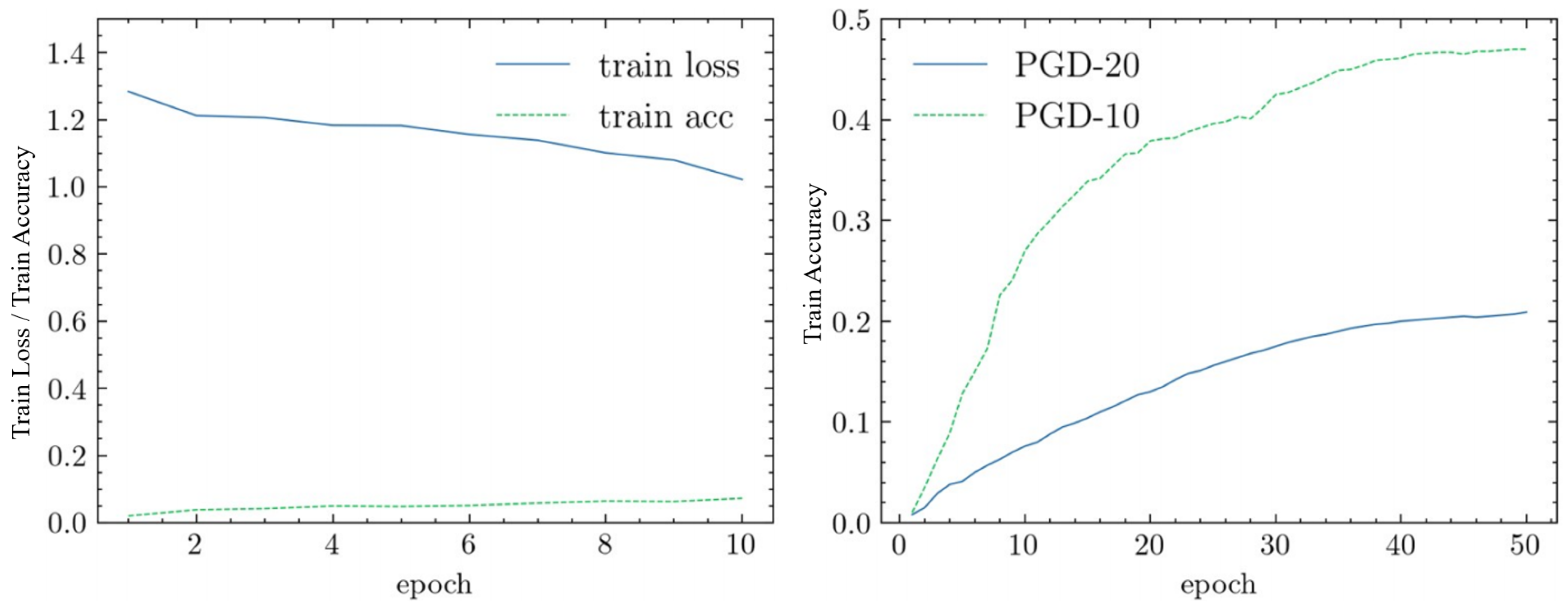
To address the issue of slow accuracy improvement and slow convergence in lightweight Transformer models during traditional adversarial training, this study adopted static parameter adjustment to enhance training efficiency. Specifically, based on traditional adversarial training, suitable values were set for the momentum and weight decay parameters of the SGD optimizer. Additionally, for the learning rate, the fixed learning rate was optimized by performing a warm-up in the early stages of adversarial training, followed by cosine annealing to cyclically adjust the learning rate based on the cosine function. This strategy better balances global and local search, improving adversarial robustness as well as the model’s performance and convergence speed during adversarial training. Furthermore, the study set appropriate PGD iteration steps and perturbation thresholds for the lightweight Transformer model to prevent the generation of low-quality adversarial examples. The model training curves before and after static parameter adjustment are shown in Figure 5.

The static parameter adjustment strategy was applied to solve the problem of slow accuracy growth and convergence during traditional adversarial training of lightweight Transformer models. Specifically, suitable values for the momentum and weight decay parameters of the SGD optimizer were set. For learning rate adjustment, a cyclical strategy was adopted to more effectively control the training process. At the start of adversarial training, a warm-up was performed by setting a small learning rate and gradually increasing it to a pre-set threshold to avoid issues with non-convergence due to an excessively high learning rate in the early stages. Subsequently, cosine annealing was employed to periodically adjust the learning rate according to the cosine function, maintaining an appropriate adjustment range during training. This strategy better balances global and local search, improving both adversarial robustness and the model’s performance and convergence speed during adversarial training. Additionally, for lightweight Transformer models, moderate PGD iterations and perturbation thresholds were set to prevent the generation of low-quality adversarial examples. After the static parameter adjustment, the convergence speed was significantly improved, accelerating model training. The model training curves are shown in Figure 5.

2. Dynamic Parameter Optimization

To address issues such as sudden increases in loss and gradient explosion during traditional adversarial training of lightweight models, this study employs dynamic parameter optimization. Specifically, gradient clipping is used to constrain the gradient updates within a reasonable range, preventing issues such as excessively large (gradient explosion) or excessively small (gradient vanishing) gradients during training. This approach ensures a more stable adversarial training process for lightweight Transformer models.

Using gradient clipping, the gradient descent process can be reformulated as shown in Equations (1) and (2). Given the objective function $f(X;\theta )$ and the learning rate $\lambda$, the parameter $\theta$ is iteratively adjusted at each step t. Let the clipping threshold be denoted by $h_d$.

$${\theta }_t={\theta }_{t-1}-\lambda h_c{\nabla }_{\theta }f(\mathbf{X},{\theta }_{t-1})$$

(1)

$$h_c=min\left({\displaystyle \frac{{\eta }_c}{∥{\nabla }_{\theta }f(\mathbf{X},{\theta }_{t-1})∥}},1\right)$$

(2)

Under the influence of the gradient clipping algorithm, the model parameter ${\theta }_0\in {\mathbb{R}}^d$ undergoes gradient descent, where each step’s descent direction is scaled by a factor of $\lambda ·h_c$. The product of these two parameters determines the step size. The operation of gradient clipping can be viewed as the process shown in Equation (3):

$${\mathrm{Clip}}_{h_c}\left({\nabla }_{\theta }f(\mathbf{X},{\theta }_{t-1})\right)={\nabla }_{\theta }f(\mathbf{X},{\theta }_{t-1})·min\left({\displaystyle \frac{{\eta }_c}{∥{\nabla }_{\theta }f(\mathbf{X},{\theta }_{t-1})∥}},1\right)$$

(3)

During gradient descent, the gradient clipping strategy effectively limits the negative impact of excessively large gradients on model performance. By restricting the maximum range of gradients, it ensures the stability of the training process, thereby helping to improve the model’s convergence speed and final performance [42].

3. Staged Model Parameter Update

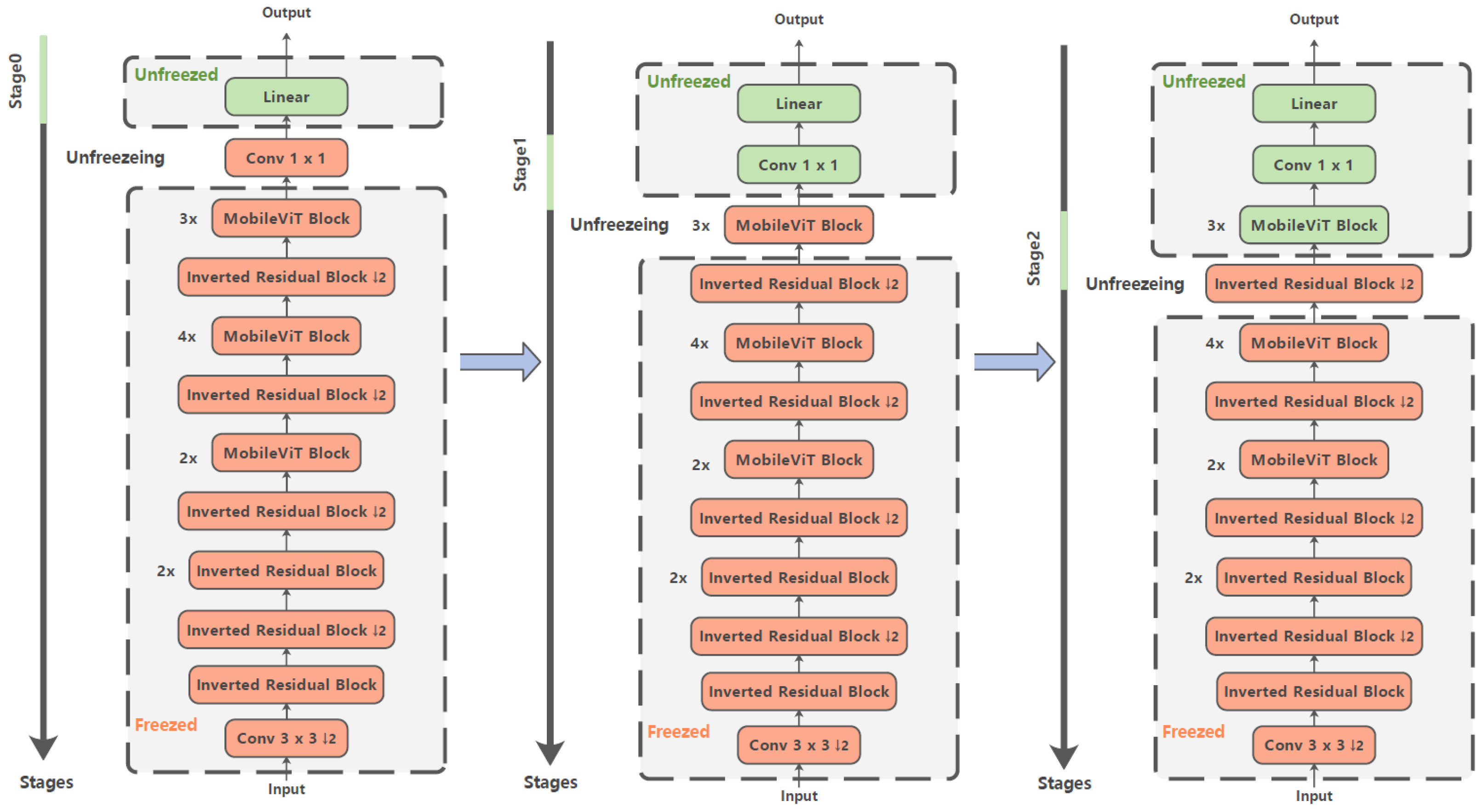
To address issues such as unstable loss convergence and overfitting during adversarial training of lightweight Transformer models, this study adopts a staged layer-wise unfreezing strategy. Initially, all layers of the model except the final layer are frozen. As training progresses, the layers are gradually unfrozen one by one. This approach helps mitigate the risk of overfitting and reduces computational cost.

The concept of layer-wise staged unfreezing was first proposed by Howard et al. [43] in the context of fine-tuning in natural language processing tasks. Inspired by this principle, our study applies it to lightweight Transformer models for visual classification tasks. By using the learning period as a unit, layers are progressively unfrozen from back to front. This method is applied to a representative lightweight Transformer model, MobileViT, as illustrated in Figure 6.

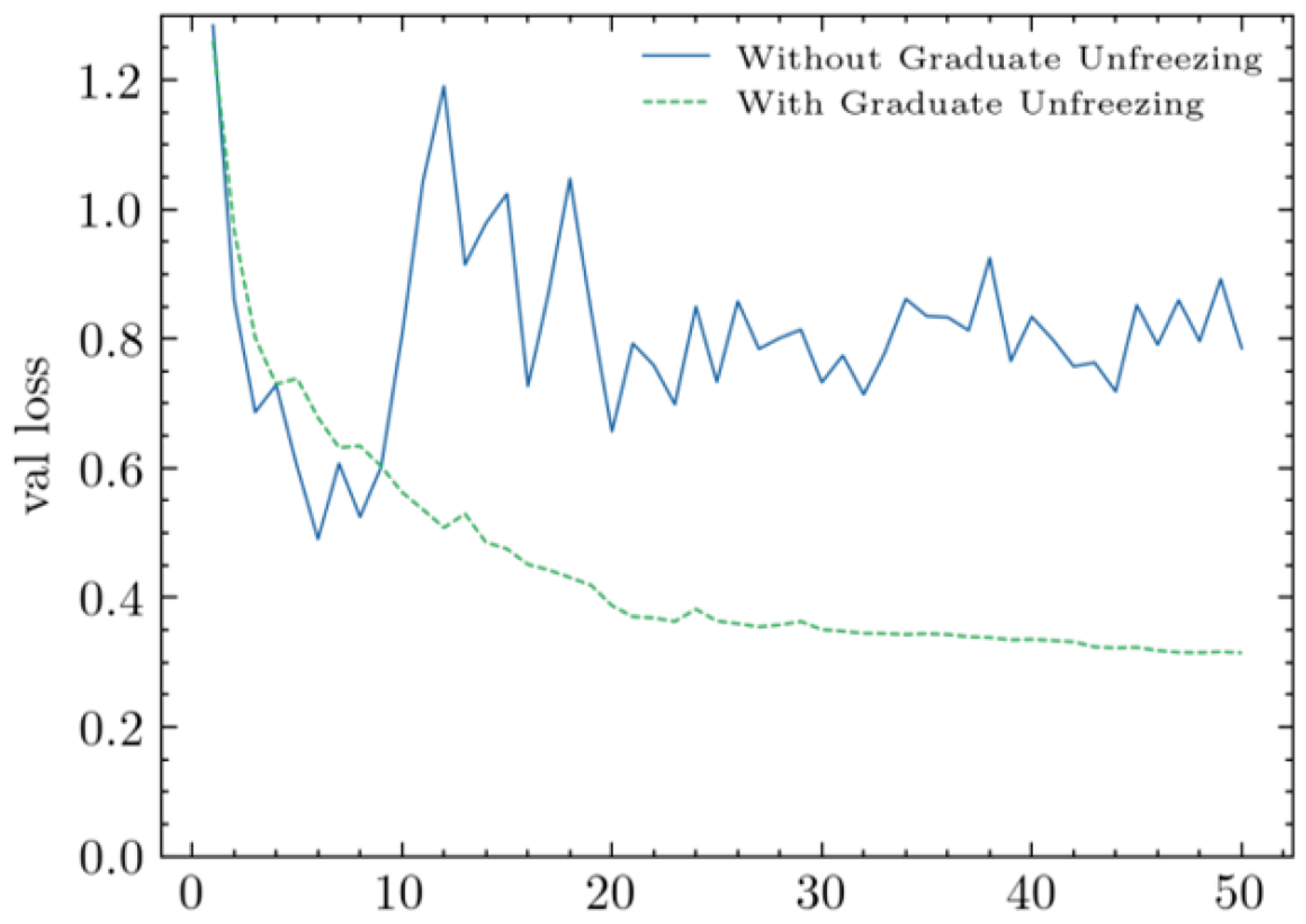
The layer-wise unfreezing method effectively alleviates issues of unstable validation loss convergence and overfitting during adversarial training of lightweight Transformer models. As shown in Figure 7, the progressive unfreezing strategy leads to smoother loss variations and eventual convergence during PGD-10 adversarial training.

4.1.2. Adversarial Training Strategy Oriented Toward Decision Boundary Optimization

1. Decision Boundary Optimization Based on TRADES

Tsipras et al. [44,45] proposed from a theoretical perspective in 2019 that constructing adversarial samples during training may degrade classification accuracy on clean examples. Therefore, there is a need to balance robustness and accuracy in adversarial training. TRADES [40,41] is a technique that improves the balance between accuracy and robustness through decision boundary optimization. Compared with conventional adversarial training, it attains a more favorable compromise between robustness and accuracy, thereby facilitating more balanced learning in machine learning models. As noted by Zhang et al. [46], the robust error (${\mathcal{R}}_{\mathrm{rob}}$) is generally composed of two elements: the natural error (${\mathcal{R}}_{\mathrm{nat}}$), measured on clean data, and the boundary error (${\mathcal{R}}_{\mathrm{bdy}}$), caused by adversarial perturbations. Thus, the total robust error can be expressed as the combination of these two sources of error, as shown in Equation (4).

$${\mathcal{R}}_{\mathrm{rob}}\left(f\right)={\mathcal{R}}_{\mathrm{nat}}\left(f\right)+{\mathcal{R}}_{\mathrm{bdy}}\left(f\right)$$

(4)

The core idea of the TRADES method is to minimize the natural error and robust error during training. While natural error reflects the model’s performance on clean samples, boundary error reflects its robustness to adversarial perturbations. By optimizing this trade-off loss, TRADES can maintain model accuracy while improving adversarial robustness.

TRADES introduces a novel loss function that jointly accounts for the classification loss on clean inputs and the robustness objective concerning adversarial examples. Specifically, the TRADES loss comprises two main components:

• Cross-entropy loss: This term targets clean data and is designed to maximize the model’s classification accuracy.
• Adversarial loss: This term evaluates how well the model maintains performance when exposed to adversarially perturbed inputs.

In TRADES, the Kullback–Leibler (KL) divergence is employed to measure discrepancies between the predicted distributions of clean and adversarial inputs. Minimizing this divergence helps the model improve its robustness against adversarial perturbations. During training, model parameters are iteratively optimized by reducing the TRADES loss through gradient descent. At each step, adversarial examples are crafted using the PGD method, followed by loss computation and parameter updates. This process is repeated over the training set until the model converges.

In this study, we adopt the TRADES framework by decomposing the adversarial training loss $L(\theta ,x,y)$ into natural loss $L_{\mathrm{CrossEntropy}}(\theta ,x,y)$ and adversarial loss $L_{\mathrm{adv}}(\theta ,x,x_{\mathrm{adv}})$. The adversarial training loss function is defined as shown in Equation (5):

$$L(\theta ,x,y)=L_{\mathrm{CrossEntropy}}(\theta ,x,y)+\beta ·L_{\mathrm{adv}}(\theta ,x,x_{\mathrm{adv}})$$

(5)

Here, $\beta$ serves as a hyperparameter that controls the trade-off between the standard classification loss and the adversarial component. The adversarial loss, introduced in Equation (5), is formulated using the KL divergence, as detailed in Equation (6).

$$L_{\mathrm{adv}}(\theta ,x,x_{\mathrm{adv}})=KL(P(·|x),P(·|x_{\mathrm{adv}}))$$

(6)

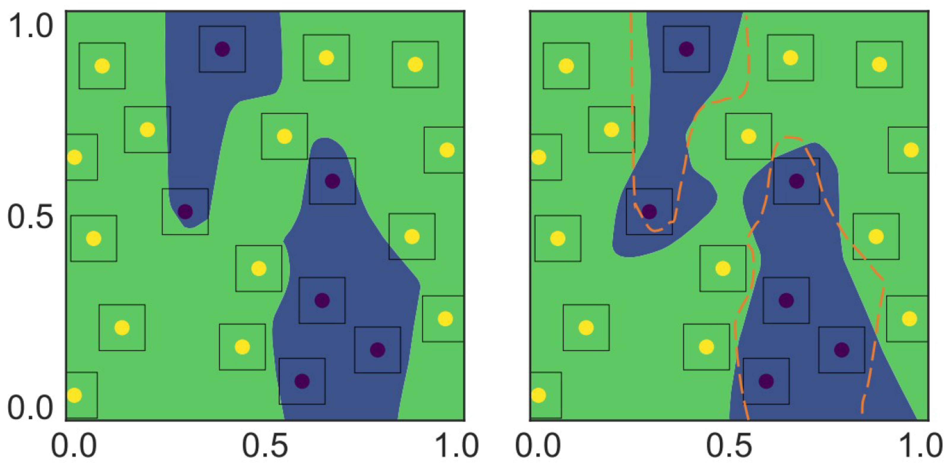
As shown in Figure 8, the image on the left represents the decision boundary trained on clean samples, while the image on the right illustrates the decision boundary obtained through the TRADES method. Although both boundaries achieve zero classification error on natural samples, TRADES achieves a more robust decision boundary by balancing robustness on clean samples and adversarial samples.

2. Decision Boundary Smoothing Based on the SMART Method

SMART [47] is a shorthand for Smoothness-inducing Adversarial Regularization and BRegman pRoximal poinT optTimization (SMART³). Proposed by Jiang et al. in 2020, SMART is a regularization method originally designed for fine-tuning NLP models. This study builds on the core concept of SMART and extends its application to the computer vision domain. We refer to our adapted version as SMART+, applying it to generate adversarial samples and conduct adversarial training to improve the robustness of lightweight Transformer models.

The core idea of SMART+ mainly consists of the following component:

(1) Smoothness-Inducing Adversarial Regularization

To address the issue of model overfitting and poor generalization due to the complexity of task-specific and domain-specific pretraining, the Smoothness-Inducing Adversarial Regularization (SIAR) method aims to solve the optimization problem defined in Equation (7):

$$\underset{\theta }{min}\mathcal{F}\left(\theta \right)=\mathcal{L}\left(\theta \right)+{\lambda }_s{\mathcal{R}}_s\left(\theta \right)$$

(7)

where $\mathcal{L}\left(\theta \right)$ denotes the conventional loss function, as specified in Equation (8).

$$\mathcal{L}\left(\theta \right)={\displaystyle \frac{1}{n}}\sum _{i=1}^n\mathsf{\ell }\left(f(x_i;\theta ),y_i\right)$$

(8)

In Equation (7), ${\lambda }_s$ is a hyperparameter, and the regularization term ${\mathcal{R}}_s\left(\theta \right)$ is defined in Equation (9):

$${\mathcal{R}}_s\left(\theta \right)={\displaystyle \frac{1}{n}}\sum _{i=1}^n\underset{\parallel {\tilde{x}}_i-x_i{\parallel }_p\le \epsilon }{max}{\mathsf{\ell }}_s\left(f({\tilde{x}}_i;\theta ),f(x_i;\theta )\right)$$

(9)

In Equation (9), $\epsilon$ denotes the radius under the $L_p$ norm, which defines the perturbation range. To minimize the objective function, it encourages the function f to vary as smoothly as possible within the $\epsilon$-ball around each input. This smoothness helps prevent model overfitting and enhances generalization. The term ${\mathsf{\ell }}_s$ in Equation (9) typically adopts symmetric KL divergence, as defined in Equation (10):

$${\mathsf{\ell }}_s(P,Q)={\mathcal{D}}_{\mathrm{KL}}(P\parallel Q)+{\mathcal{D}}_{\mathrm{KL}}(Q\parallel P)$$

(10)

This method introduces a smoothness-inducing regularization step during fine-tuning, which effectively controls model complexity. Moreover, by incorporating adversarial samples and comparing the classifier output distributions of adversarial and clean samples, the method enables the model to acquire a certain level of robustness against adversarial examples.

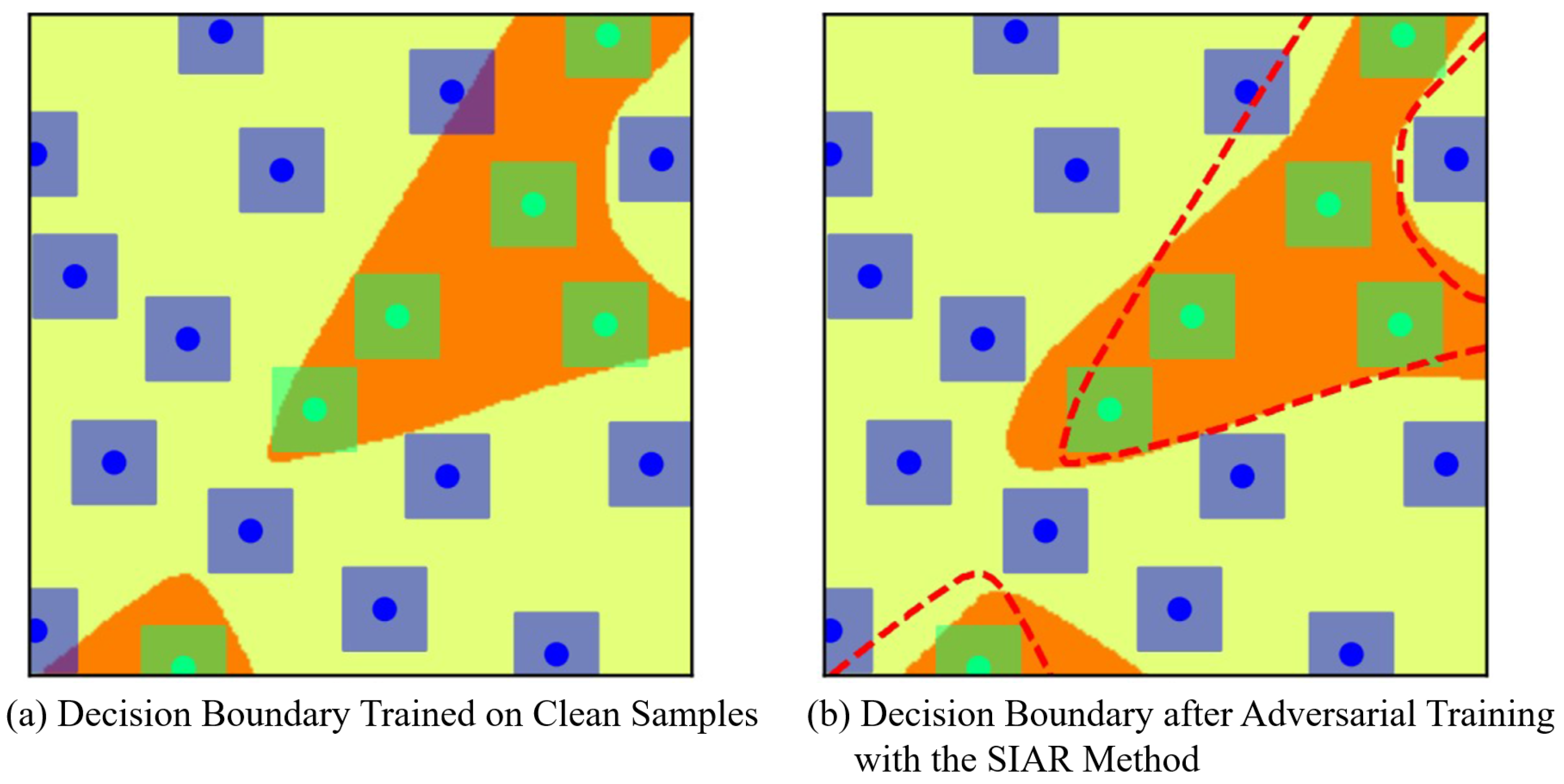
As shown in Figure 9, the left image depicts the decision boundary trained on clean samples, while the right image shows the decision boundary after applying adversarial training with the SIAR method. It can be observed that the SIAR method smooths the decision boundary during adversarial training, thereby enhancing the model’s discriminative capability. Moreover, for two similar input samples, a smoother decision boundary leads to more consistent prediction results.

(2) Bregman Proximal Point Optimization

To solve the optimization problem in Equation (7), the SMART+ method introduces trust region optimization based on the traditional Bregman Proximal Point method by incorporating a momentum-like prior. In this study, we define the pretrained initialization model as $f(·;{\theta }_0)$. At the $(t+1)$-th iteration, the parameters are updated using the traditional Bregman Proximal Point method as shown in Equation (11):

$${\theta }_{t+1}=arg\underset{\theta }{min}\mathcal{F}\left(\theta \right)+\mu {\mathcal{D}}_{\mathrm{Breg}}(\theta ,{\theta }_t)$$

(11)

In Equation (11), $\mu$ is a hyperparameter, and ${\mathcal{D}}_{\mathrm{Breg}}(\theta ,{\theta }_t)$ denotes the Bregman divergence, defined in Equation (12):

$${\mathcal{D}}_{\mathrm{Breg}}(\theta ,{\theta }_t)={\displaystyle \frac{1}{n}}\sum _{i=1}^n{\mathsf{\ell }}_s\left(f(x_i;\theta ),f(x_i;{\theta }_t)\right)$$

(12)

The Bregman divergence in the traditional Bregman Proximal Point method serves as a regularization term during each iteration, preventing the model’s parameters ${\theta }_{t+1}$ from drifting too far from those of the previous iteration. Therefore, the method effectively preserves the knowledge learned during pretraining, particularly knowledge derived from out-of-distribution (OOD) data.

Since the optimization problem in Equation (11) does not have a closed-form solution, we adopt the ADAM optimizer to solve it using stochastic gradient descent. Instead of solving Equation (11) until convergence in each iteration, we only perform a few update steps to generate a reliable initialization for the next subproblem.

Building upon the traditional Bregman Proximal Point framework, the SMART+ method accelerates optimization by introducing a momentum-based iterative update scheme, as shown in Equation (13):

$${\theta }_{t+1}=arg\underset{\theta }{min}\mathcal{F}\left(\theta \right)+\mu {\mathcal{D}}_{\mathrm{Breg}}(\theta ,{\tilde{\theta }}_t)$$

(13)

In Equation (13), ${\tilde{\theta }}_t=(1-\beta ){\theta }_t+\beta {\tilde{\theta }}_{t-1}$, where $\tilde{\theta }$ represents the exponential moving average, and $\beta$ is a momentum parameter in the interval $(0,1)$.

During adversarial training, the SMART+ method utilizes a local smoothness regularization term to generate adversarial examples. This regularization term computes the output difference between clean and adversarial inputs, encouraging the model to produce similar outputs for nearby inputs. In each training iteration, the SMART+ method updates the model parameters by minimizing this regularized loss function.

The adversarial training process adopts the ADAM optimizer to update model parameters, performing T rounds of updates in total. The specific training process is shown in Algorithm 1.

Algorithm 1 SMART+: Adversarial Training Strategy Combining Smoothness-Inducing Regularization and Momentum-Accelerated Bregman Proximal Optimization

Require: Number of iterations T, dataset $\mathcal{X}$, pretrained model parameters ${\theta }_0$, Gaussian noise variance ${\sigma }^2$, learning rate $\eta$, momentum parameter $\beta$, batch size $BS$ Ensure: Model parameters ${\theta }_T$ after T iterations   1: ${\tilde{\theta }}_1\leftarrow {\theta }_0$   2: for $t=1$ to T do   3:     $\overline{\theta }\leftarrow {\tilde{\theta }}_{t-1}$   4:     Randomly sample a batch $\mathcal{B}$ of size $BS$ from $\mathcal{X}$   5:     for $i=1$ to $BS$ do   6:         ${\tilde{x}}_i\leftarrow x_i+v_i$                ▹$v_i\sim \mathcal{N}(0,{\sigma }^{2}I)$   7:         ${\tilde{h}}_i\leftarrow {\displaystyle \frac{1}{\left|\mathcal{B}\right|}}{\sum }_{x_j\in \mathcal{B}}{\nabla }_{{\tilde{x}}_i}{\mathsf{\ell }}_s\left(f({\tilde{x}}_i;\overline{\theta }),f({\tilde{x}}_j;\overline{\theta })\right)$   8:         ${\tilde{g}}_i\leftarrow {\displaystyle \frac{{\tilde{h}}_i}{\parallel {\tilde{h}}_i{\parallel }_2}}$   9:         ${\tilde{x}}_i\leftarrow {\Pi }_{\parallel {\tilde{x}}_i-x_i{\parallel }_p\le ϵ}\left({\tilde{x}}_i+\eta {\tilde{g}}_i\right)$     ▹${\Pi }_A$ denotes projection onto set A 10:     end for 11:     Feed adversarial samples $\tilde{\mathcal{B}}$ into the model 12:     Update $\overline{\theta }$ using Adam: $\overline{\theta }\leftarrow \mathrm{AdamUpdate}\left(\overline{\theta }\right)$ 13:     ${\theta }_t\leftarrow \overline{\theta }$ 14:     ${\tilde{\theta }}_{t+1}\leftarrow (1-\beta )\overline{\theta }+\beta {\tilde{\theta }}_t$ 15: end for

In the above process, this study adopts a smoothness-inducing regularization approach to generate adversarial samples, which are constrained within an $\epsilon$-neighborhood of the clean samples. To solve the optimization problem in Equation (7), this study further employs the Bregman Proximal Point method.

In addition, momentum is introduced, and the exponential moving average method is used to accelerate the iterative optimization process across multiple updates.

4.1.3. Hyperparameter Ablation

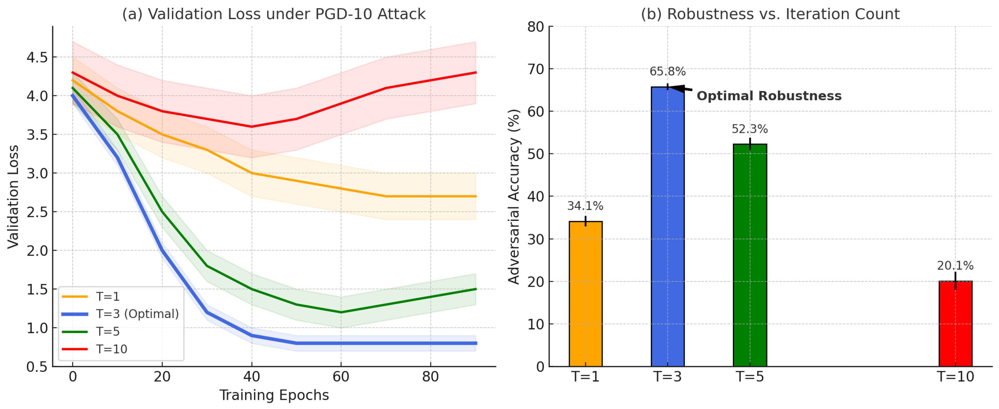
To determine the optimal number of iterations T for adversarial sample generation in the SMART+ method, we designed systematic ablation experiments. Under fixed values for other hyperparameters ($ϵ=2/255$, $\beta =0.9$, ${\sigma }^2=0.01$), we conducted comparative evaluations for $T\in 1,3,5,10$. The experiments were conducted on the MobileViT-s model and the CIFAR-10 validation set, using two key indicators:

(1) Training Stability: Validation loss curve under PGD-10 attack.

(2) Robustness Improvement: Classification accuracy on adversarial samples.

Experimental results are shown in Figure 10, and the results show the following: (1) $T=1$: The validation loss exhibits severe oscillation (orange curve), indicating insufficient adversarial sample generation and inadequate decision boundary smoothing (corresponding robust accuracy is only 34.15%). (2) $T=3$: The loss curve converges smoothly to the lowest value (blue curve), and robust accuracy reaches its peak at 65.77%. (3) $T\ge 5$: The loss curve shows a trend of dispersion (red/purple curves), and for $T=10$, robust accuracy drops sharply to 20.12%, demonstrating that excessive iterations lead to overfitting.

Due to the limited capacity of lightweight models (e.g., MobileViT-s with only 5.5 M parameters), when $T>3$, multiple iterative updates cause adversarial samples to move outside the effective perturbation region ($ϵ$-ball); the generated samples deviate excessively from the distribution of real data, violating the local smoothing assumption (Equation (9)); and the model overfits to invalid perturbations, undermining its regularization ability (Equation (7), ${\mathcal{R}}_s\left(\theta \right)$ fails).

Therefore, $T=3$ achieves the optimal balance between decision boundary smoothing and training efficiency, which is especially suitable for resource-constrained scenarios.

4.2. Robustness Evaluation of Lightweight Transformers Under Resource-Constrained Scenarios

This study first adopts traditional adversarial training techniques and, through a series of stable training strategies and efficiency-enhancing methods, obtains lightweight Transformer models with initial robustness. However, conventional adversarial training methods often exhibit significant performance degradation when applied to lightweight Transformer models. To address the trade-off between clean accuracy and adversarial robustness, we employ the TRADES method, which significantly enhances model robustness while also maintaining or even improving clean-sample classification accuracy.

In addition, we integrate the SMART method—originally proposed in the NLP domain—and extend its core idea to the adversarial training of lightweight Transformers. By applying different adversarial sample generation techniques across training iterations, we perform adversarial training on lightweight Transformer models. Under a 3-iteration adversarial training scheme, we obtain a Transformer model with high robustness and low complexity.

In our experiments, the lightweight Transformer model trained using TRADES demonstrates strong robustness. Furthermore, in real-world resource-constrained scenarios—particularly on mobile devices—we successfully deploy the model inference pipeline and perform robust inference with the lightweight Transformer model.

4.2.1. Deployment of Lightweight Transformer Models on Mobile Devices

In this study, we selected a mobile device suited for resource-constrained environments—Xiaomi 11—for deployment. By integrating the Expo platform with PlayTorch, we enabled the execution of a lightweight Transformer model based on PyTorch on mobile phones to perform classification tasks.

Expo is an open-source frontend framework that runs on Android, iOS, and Web platforms. We used it to build a lightweight Transformer model prediction application.

When deploying deep learning models to mobile or edge devices, there are typically three options: TensorFlow Lite, TensorFlow.js, and PlayTorch. TensorFlow Lite is suitable for deploying models on mobile devices, while TensorFlow.js enables deployment on Web applications. Considering that all adversarial training in this study is based on the PyTorch framework, we chose PlayTorch, which natively supports PyTorch.

PlayTorch is powered by PyTorch Mobile and React Native. It allows Expo and similar frontend frameworks to load corresponding SDKs and remotely invoke PyTorch services on mobile devices, enabling the construction of customized image classification models, as illustrated in Figure 11.

To deploy a mobile deep learning application based on PlayTorch, the typical steps are as follows:

• Create a new mobile project: Use Expo Snack to initialize a new Expo project from a template.
• Add PlayTorch dependencies: In the package.json file of the project, include dependencies such as react-native-pytorch-core and react-native-safe-area-context.
• Handle image input: On mobile devices, images can be input either by selecting files locally or via the camera. Once the image is captured, it needs to be converted into a format the model can process—a tensor (multi-dimensional array). For lightweight Transformer models, the image must be resized and transformed into a 256 × 256 tensor of a specific shape.
  To do this, first import torch, torchvision, and media from react-native-pytorch-core. Then use torchvision.transforms to create a transform object. Define a function classifyImage that reads the image, converts it to a blob, and then to a tensor. After center-cropping and resizing the tensor, feed it into the model.
• Run inference: Import the MobileModel package, create a variable model to store the model, and initialize it using MobileModel.load(). To make predictions, pass the tensor to the model using model.forward(tensor) to obtain the output.
• Display classification results: Since the model outputs a numeric value, a topClass dictionary is defined to map output values to actual category labels. The final output is the corresponding label predicted by the model.

4.2.2. Robustness Evaluation of Lightweight Transformer Models on Mobile Devices

After deploying the model inference system on an Android device, the adversarial robustness of lightweight Transformer architectures can be assessed. The evaluation procedure is as follows:

• Select clean input samples that the lightweight Transformer model can classify correctly prior to training, and apply common white-box attacks such as FGSM and PGD to craft adversarial examples.
• Load both the adversarially trained model weights $W_1$ and the standard pretrained weights $W_0$ into the mobile application, then feed the adversarial examples into each model independently.
• Compare the prediction outcomes of the two models on the adversarial inputs, and compute the top-3 consistency across their outputs.

5. Experimental Findings and Evaluation

This section details the robustness assessments of lightweight Transformer models at three hierarchical levels. It also provides a comprehensive examination of their robustness properties and highlights the improvements realized through the implementation of the proposed adversarial training methods.

The section reports experimental results from two perspectives: stable adversarial training and decision-boundary-oriented optimization, analyzing the effectiveness of the proposed adversarial training methods. Finally, the section illustrates the deployment and robustness inference of lightweight Transformer models under real-world low-resource scenarios, validating the feasibility of the proposed adversarial training framework.

5.1. Evaluation Results and Analysis of Lightweight Transformer Model Robustness

Above, this study proposed a robustness evaluation framework for visual Transformers across three levels: noise robustness, data robustness, and adversarial robustness. Based on this framework, we conduct multi-level evaluations of lightweight Transformer models in this section.

5.1.1. Model Selection

This study selects a lightweight and efficient Transformer model—MobileViT—as the representative of lightweight Transformers. Meanwhile, Vision Transformer (ViT), a widely used backbone in computer vision, is chosen as the baseline for comparison. A comprehensive evaluation is conducted to compare the robustness of the two types of models, analyzing their performance under various robustness evaluation criteria.

To investigate how model scale influences robustness under comparable architectural designs, we examine three configurations of the Vision Transformer: ViT-Base, ViT-Small, and ViT-Tiny. In parallel, we choose three MobileViT models with varying parameter sizes: MobileViT s, MobileViT xs, and MobileViT xxs. As shown in

Table 2. Model selection and parameters for Transformer robustness evaluation.

Model Name	Number of Parameters	Number of Parameters (Million)
vit base patch16 224	102,443,859	102.4
vit small patch16 224	21,974,632	21.9
vit tiny patch16 224	5,679,400	5.6
mobilevit s	5,566,376	5.5
mobilevit xs	2,309,400	2.3
mobilevit xxs	1,267,912	1.2

, ViT tiny has a similar parameter size to MobileViT s, whereas the other ViT variants differ significantly in model size compared to MobileViT. All models are pretrained on the ILSVRC2012 [48] dataset.

5.1.2. Noise Robustness Evaluation Results and Analysis

Since both ViT and MobileViT models were initialized using pretrained weights from the ImageNet-1k dataset, this study utilizes Tiny-ImageNet-C as the corruption evaluation benchmark. The source dataset for Tiny-ImageNet-C, known as Tiny-ImageNet-200, originates from a subset of the ImageNet-1k validation data.

To mitigate the influence of distributional discrepancies in the experiments, we fine-tune both ViT and MobileViT models on the Tiny-ImageNet-200 dataset. Following this step, we assess the effectiveness of all six models on Tiny-ImageNet-C across different noise corruption types. The corresponding results can be found in

Table 3. Noise robustness performance of ViTs and MobileViTs on Tiny-ImageNet-C.

Model Name	Number of Params	Clean Error	mCE	$\mathbf{\Delta }$
vit base patch16 224	102.4 M	15.18%	37.60%	22.42%
vit small patch16 224	21.9 M	15.06%	39.92%	24.68%
vit tiny patch16 224	5.6 M	24.16%	54.72%	30.56%
mobilevit s	5.5 M	23.19%	61.13%	37.94%
mobilevit xs	2.3 M	28.95%	65.48%	36.53%
mobilevit xxs	1.2 M	38.02%	70.04%	32.02%

.

In addition, we adopt the evaluation metric proposed by Hendrycks et al., called the mean Corruption Error (mCE), which measures the average impact of all corruption types. The mCE is calculated for Equation (14), where the number of corruption types $n=15$:

$$\mathrm{mCE}={\displaystyle \frac{1}{n}}\sum _{i\in \mathrm{Corruption}\mathrm{Set}}{\mathrm{Error}}_i$$

(14)

In terms of noise robustness, based on the results in Table 3 and Equation (14), we observe that higher-capacity ViT models generally demonstrate better noise robustness. For models with the same architecture, those with more parameters tend to achieve stronger robustness against noise.

In addition, ViT and MobileViT models exhibit different trends in clean-vs.-corrupted error rate gaps. Specifically, ViT models show increasing error gaps as parameter count decreases, while MobileViT models show decreasing gaps as parameter count reduces. In extreme cases, the smallest MobileViT model, with only 1.17% of the parameters of the ViT model, achieves 72.97% clean accuracy, whereas the largest MobileViT model (5.3% of ViT’s parameters) reaches 90.43% clean accuracy. This indicates that MobileViT achieves good classification performance even under high compression.

However, for corrupted samples, under the same extreme condition (1.17% of ViT parameters), the MobileViT model achieves only 48.01% noise robustness accuracy, compared to 72.97% for ViT. Even when MobileViT is scaled up to 5.3% of ViT’s size, its noise robustness accuracy remains at 72.56%, significantly lower than ViT. This suggests that excessive compression can hurt model robustness. Finally, as shown in Figure 12, both MobileViT and ViT models exhibit similar trends in robustness accuracy across different corruption types on Tiny-ImageNet-C, implying that the Transformer backbone offers relatively strong control over model robustness across noise conditions.

5.1.3. Data Robustness Evaluation Results and Analysis

In terms of data robustness, there is a significant performance gap between ViT and MobileViT models on clean datasets such as ImageNet-R and ImageNet-Sketch. This indicates that model compression in the lightweighting process notably degrades the data robustness of Transformer models.

However, for datasets with distributional shifts (e.g., ImageNet-R and ImageNet-Sketch), the accuracy gap between ViT and MobileViT begins to narrow. Notably, the highly compressed MobileViT s model even outperforms the ViT tiny model in terms of data robustness. Further investigation of classification errors on clean versus distribution-shifted data (as shown in Figure 12c) reveals that the error variation patterns of MobileViT and ViT largely overlap, and the accuracy gap between them narrows further under distributional shift.

One possible explanation is that MobileViT’s hybrid architecture—featuring both local and global representations—allows it to better adapt to data shifts. Another plausible interpretation is that since MobileViT combines CNN and Transformer structures, it inherits the low-sensitivity, high-generalization characteristics of CNNs, especially under data perturbation. Therefore, when data distribution shifts, MobileViT models tend to be more robust than ViTs. However, due to architectural and parameter limitations, MobileViT still cannot outperform ViT in overall data robustness.

5.1.4. Adversarial Robustness Evaluation Results and Analysis

For ViT and MobileViT models initialized with weights from the ImageNet-1k dataset, we assess their adversarial robustness using the ImageNet-1k validation set and the CIFAR-10 benchmark. The evaluation employs a perturbation limit of $ϵ=8/255=0.031$. The procedure for adversarial testing is as follows:

• From the selected datasets (ImageNet-1k validation and CIFAR-10), extract a predefined quantity of correctly classified clean samples per class to construct the clean dataset ${\mathcal{D}}_{\mathrm{clean}}$.
• Use three adversarial attack methods—FGSM, PGD, and MIM—to generate adversarial examples from ${\mathcal{D}}_{\mathrm{clean}}$, resulting in the adversarial dataset ${\mathcal{D}}_{\mathrm{adv}}$.
• Feed ${\mathcal{D}}_{\mathrm{adv}}$ into both ViT and MobileViT models and compute the classification accuracy to evaluate their adversarial robustness.

The adversarial robustness results are shown in

Table 4. Performance of ViTs and MobileViTs under FGSM, PGD, and MIM Attacks.

Model Name	ImageNet			CIFAR-10
	FGSM	PGD	MIM	FGSM	PGD	MIM
vit base patch16 224	27.9%	0.7%	1.3%	33.5%	1.9%	2.3%
vit small patch16 224	21.2%	0.4%	0.7%	28.4%	2.0%	1.8%
vit tiny patch16 224	15.1%	0.0%	0.0%	20.9%	0.6%	0.2%
mobilevit s	12.9%	0.0%	0.0%	17.3%	0.0%	0.0%
mobilevit xs	8.3%	0.0%	0.0%	12.1%	0.0%	0.0%
mobilevit xxs	3.6%	0.0%	0.0%	10.9%	0.0%	0.0%

.

In terms of adversarial robustness, it is noteworthy that the lightweight MobileViT models consistently outperform the ViT tiny model in classification accuracy, regardless of whether clean or adversarial samples are used. On the ImageNet-A clean dataset, the classification accuracy gap between MobileViT and ViT models is relatively small. For example, MobileViT xxs, which has only 1.17% of the parameters of ViT base, shows a clean accuracy gap of only about 5%, further demonstrating the efficiency of MobileViT in lightweight scenarios.

However, under adversarial attacks, although ViT models show a significant drop in accuracy, the MobileViT models exhibit an even sharper decline. Compared to ViTs, the MobileViT accuracy drops an additional 20%, indicating that adversarial robustness significantly deteriorates with aggressive model compression.

As shown in Figure 12b, the classification accuracy of MobileViT models under adversarial attacks drops to below 10%—with the worst model achieving less than 5%, which is only a fraction (15% to 30%) of the optimal ViT model performance.

Moreover, Table 4 clearly shows the vulnerability of MobileViT models under various attack methods. Under FGSM, MobileViT suffers a large drop, with the worst-case accuracy reaching just 46.23% on ImageNet and 51.64% on CIFAR-10. Under stronger attacks like PGD and MIM, although ViT models can still recognize some adversarial samples, MobileViT models nearly lose their ability to correctly classify them. In conclusion, lightweight models exhibit serious deficiencies in terms of adversarial robustness.

5.2. Results and Analysis of Robustness Improvement via Adversarial Training

5.2.1. Results and Analysis of Stable Traditional Adversarial Training

To improve the adversarial resilience of compact Transformer architectures, we begin by applying standard adversarial training techniques. In this approach, two widely used white-box attack algorithms, FGSM and PGD, are employed to craft adversarial examples using clean inputs and model gradients. These generated examples are incorporated into the training dataset to lessen the model’s vulnerability to adversarial noise and strengthen its robustness.

Specifically, we choose the CIFAR-10 dataset and select three MobileViT variants with different model sizes: MobileViT_s, MobileViT_xs, and MobileViT_xxs (all pretrained on ImageNet-1k). The adversarial training is conducted using the conventional $L_{\infty }$ norm attack. For each clean input x, we generate an adversarial sample $x_{\mathrm{adv}}$ such that $\parallel x-x_{\mathrm{adv}}{\parallel }_{\infty }\le ϵ$. The perturbation limit was fixed at $ϵ=8/255$ in our experiments.

To generate adversarial inputs, we utilized both FGSM and PGD methods. PGD was configured with 20 iterations ($t=20$) and a step size of $2/255$. The model was trained using the cross-entropy loss function, and stochastic gradient descent (SGD) served as the optimizer.

However, during traditional adversarial training of lightweight Transformer models, several issues arise, including slow convergence, overfitting, and prolonged preprocessing time for image input and evaluation. To address these challenges, we introduce multiple strategies to further accelerate and stabilize the adversarial training process.

1. Training Results and Analysis of Different Stabilized Adversarial Training Methods

In this study, we adopt traditional adversarial training methods, where adversarial examples generated using white-box attacks (FGSM and PGD) are input into lightweight Transformer models to improve robustness. However, relying solely on traditional adversarial training leads to numerous issues when applied to MobileViT models. These include: unstable validation loss, gradient explosion, overfitting, poor convergence, degraded accuracy, and slow model convergence speed.

To address these issues, we introduce three training stabilization strategies and design a multi-stage optimization framework to improve adversarial training performance.

Specifically, we use the DALI framework to significantly reduce training time and improve efficiency. Since lightweight Transformer models are prone to gradient explosion and validation loss oscillation during adversarial training, we apply gradient clipping to all models to mitigate this issue.

In addition,

Table 5. Adversarial robustness of MobileViTs after FGSM and PGD training (CIFAR-10).

Model	Method	Clean	Without Training	FGSM	PGD-10
MobileViT_s	GC	-	-	40.32%	44.54%
	GC+GU	83.29%	2.5%	42.78%	47.22%
	GC+GU+DLR	-	-	43.14%	47.59%
MobileViT_xs	GC	79.12%	0.0%	37.58%	42.20%
	GC+GU	-	-	39.71%	43.14%
MobileViT_xxs	GC	77.82%	0.0%	35.41%	37.94%
	GC+GU	-	-	38.39%	39.02%

GC: Gradient clipping. GU: Gradual unfreezing. DLR: Dynamic learning rate.

presents the adversarial training results on the CIFAR-10 dataset using three enhanced strategies built upon traditional training. Each method aims to provide more stable and effective adversarial training for lightweight Transformer models.

As indicated by the results in Table 5, in contrast to adversarial training that solely relies on gradient clipping, incorporating both gradient clipping and progressive unfreezing significantly boosts adversarial accuracy in lightweight architectures. Furthermore, the findings suggest that models possessing more parameters generally maintain stronger adversarial robustness. However, during the model compression process, a certain degree of adversarial robustness loss is inevitable.

2. Results and Analysis of GPU-Accelerated Training Process

In adversarial training, beyond addressing unstable convergence, generating adversarial samples through multi-step Projected Gradient Descent (PGD) is computationally expensive. Upon deeper profiling, we identify that the primary bottleneck lies in data preprocessing—particularly the resizing of CIFAR-10 images.

The original CIFAR-10 images are $32\times 32$, while lightweight Transformer models like MobileViT require inputs resized to $256\times 256$. This resizing operation, typically executed via the resize function in the PyTorch framework, significantly increases the computational burden. Our tests show that using torchvision to process and load these images consumes substantial CPU time and keeps the GPU underutilized, leading to inefficient training.

To solve this, we adopt NVIDIA’s DALI (Data Loading Library), a high-performance data preprocessing and loading library. DALI enables GPU-accelerated execution of tasks like resizing, cropping, and flipping, which are traditionally CPU-bound, thereby improving training throughput. DALI supports multi-threaded pipelines and asynchronous processing, allowing both the CPU and GPU to work concurrently, reducing data transfer latency and boosting overall training efficiency.

To evaluate DALI’s performance, we compare the training acceleration effects of using DALI versus standard PyTorch in both theory and practice. Specifically, we construct a DALI data pipeline that resizes CIFAR-10 images to $256\times 256$, and measure the time required to preprocess and load one epoch of training and test data. We also apply torchvision’s transforms.Resize to serve as a baseline for comparison. Using PyTorch 2.7.1 dataloader, we measure the epoch-wise data preprocessing and loading time. The evaluation results are reported in

Table 6. Theoretical performance comparison of data preprocessing and loading: DALI vs. PyTorch.

	DALI	PyTorch	DALI/PyTorch
Train	1.101404 s	26.181577 s	4.21%
Test	0.134144 s	2.385551 s	5.62%
Total	1.235548 s	28.567127 s	4.32%

, comparing theoretical and empirical outcomes.

From the above theoretical evaluation, it is evident that DALI completes high-efficiency data preprocessing and loading with only 4.32% of the time required by PyTorch under the same hardware conditions. Therefore, this study applies DALI to the adversarial training of MobileViT models. In practical scenarios, DALI successfully reduces the time required for one epoch of PGD-10 adversarial training from 90 min (under PyTorch) to 45 min—effectively cutting the training time in half. This result significantly improves the efficiency of model training and strongly supports the acceleration of adversarial training for lightweight Transformer models.

5.2.2. Results and Analysis of Decision Boundary Optimization Based on TRADES

1. Results and Analysis of Decision Boundary Optimization Based on TRADES

By applying the loss function defined in Equation (5) to PGD-based adversarial training, we achieved outstanding performance, as shown in

Table 7. Adversarial training results with TRADES under PGD-5 and PGD-10.

Model	PGD-5		PGD-10
	Clean Val Acc	Robust Val Acc	Clean Val Acc	Robust Val Acc
MobileViT_s	89.75%	77.91%	92.38%	81.29%
MobileViT_xs	85.29%	75.13%	89.25%	78.32%
MobileViT_xxs	82.67%	72.64%	86.03%	75.94%

.

Based on the findings presented in Table 7, the TRADES loss—which integrates natural classification and adversarial training objectives through suitable weighting—achieves a balanced compromise between standard accuracy and robustness to adversarial attacks. In comparison with conventional adversarial defense strategies, this method markedly enhances robustness against adversarial inputs.

Moreover, the model also exhibits improved classification accuracy on the validation set, further demonstrating the benefit of decision-boundary-aware adversarial training optimization.

2. Decision Boundary Smoothing Based on the SMART Method

Based on the principles of SMART, this study adopts a localized smoothness-inducing regularization approach to generate adversarial examples. The SMART+ method incorporates Bregman Proximal Point Optimization and introduces momentum-based iterative updates to generate adversarial samples within the $\epsilon$-neighborhood of the input image. These adversarial samples are then fed into the model to enhance robustness within a specified perturbation range.

Furthermore, this study evaluates the impact of different numbers of update iterations under the SMART method, using a perturbation budget of $\epsilon =2/255$ and a step size of $\mathrm{step}\mathrm{size}=2/255\times 1/5$. The results are presented in

Table 8. Adversarial training results using the SMART+ method.

Model	SMART+ Val Accuracy
	Iteration = 1	Iteration = 3	Iteration = 10
MobileViT_s	34.15%	65.77%	20.12%
MobileViT_xs	30.07%	63.14%	17.86%
MobileViT_xxs	26.54%	61.21%	14.23%

.

Analysis of Table 8 indicates that the SMART approach obtains optimal adversarial robustness when the update step count is configured to 3. In this case, the adversarial robustness outperforms all traditional adversarial training baselines.

However, when the iteration number is 1, the adversarial robustness of MobileViT is relatively weak. As the iteration number increases significantly beyond 3, such as in the case of 10 iterations, the robustness performance of the model drops noticeably—sometimes even falling below that of the 1-iteration setting and traditional adversarial training methods. Therefore, to effectively enhance robustness using the SMART method, it is crucial to precisely control the number of update iterations to achieve the best adversarial robustness.

As shown in

Table 9. Classification accuracy on adversarial examples before and after applying stability strategies.

Model	Params	Without Adv Train		Adversarial Trained
		FGSM	PGD	FGSM	${\Delta }_{\mathbf{0}}$	PGD	${\Delta }_{\mathbf{1}}$
MobileViT-s	5.7 M	17.3%	0%	43.14%	25.84%	47.59%	47.59%
MobileViT-xs	4.9 M	12.1%	0%	39.71%	27.61%	43.14%	43.14%
MobileViT-xxs	2.3 M	10.9%	0%	38.39%	27.49%	39.02%	39.02%

, the classification accuracy of MobileViT without adversarial training is only 17.3% under FGSM attack, and nearly 0% under PGD attack, indicating its vulnerability to adversarial perturbations.

However, after applying the stability-oriented adversarial training strategies proposed in this study, the adversarial robustness of MobileViT improves significantly. For example, MobileViT-xxs achieves a classification accuracy of 38.39% under FGSM attack, with a robustness gain of 27.49%, clearly enhancing the model’s resistance to perturbations. Notably, after adversarial training, MobileViT achieves a robust accuracy of 47.59% under PGD attack—the highest among all cases—demonstrating the effectiveness of the proposed strategy in improving the robustness of lightweight Transformer models.

As shown in

Table 10. Classification accuracy on adversarial samples using stability strategies and decision boundary optimization.

Model	Params	Traditional		Decision Boundary Optimized
		FGSM	PGD	SMART+	${\Delta }_{\mathbf{2}}$	TRADES	${\Delta }_{\mathbf{3}}$
MobileViT-s	5.7 M	43.14%	47.59%	65.77%	18.18%	81.29%	33.7%
MobileViT-xs	4.9 M	39.71%	43.14%	63.14%	20.0%	78.32%	35.18%
MobileViT-xxs	2.3 M	38.39%	39.02%	61.21%	22.19%	75.94%	36.92%

, compared with traditional adversarial training methods, the decision boundary optimization strategies proposed in this study have further enhanced model robustness. Specifically, the SMART+ method introduces local smoothness regularization, which not only retains the benefits of traditional adversarial training but also provides an additional boost in robustness. Notably, for the MobileViT-xxs model, the classification accuracy on adversarial examples improved by 22.19% compared to traditional training.

On the other hand, the TRADES method balances clean and adversarial classification accuracy by optimizing the loss function, significantly improving adversarial robustness even under partial drops in clean accuracy. Particularly for the MobileViT-xxs model, TRADES increased adversarial robustness by 36.92% over the traditional baseline.

5.3. Robustness Evaluation of Lightweight Transformer Models on Mobile Devices

In this study, an Android device—specifically, a Xiaomi 11 smartphone—was selected as the evaluation platform under a low-resource scenario. The robustness of lightweight Transformer models was assessed using the following procedure:

• Select a set of clean samples that can be correctly classified by the MobileViT model before and after training. Use common white-box attack methods such as FGSM and PGD to generate adversarial examples.
• Load the adversarially trained model weights ${\mathcal{W}}_1$ and the pretraining model weights ${\mathcal{W}}_0$ onto the mobile app, and respectively feed adversarial samples into the two models.
• Collect classification results for adversarial examples from both models and compare them with the top-3 results on clean samples to compute confidence-based consistency.
• Finally, take a PGD-5 generated adversarial sample and input it into both the adversarially trained and untrained MobileViT models on the mobile device. The resulting classification outcomes are shown in Figure 13.

In the inference interface, the input adversarial image and the visualized Attention Map from the MobileViT model are displayed. Two image input methods are supported: camera capture and local file upload. Below the input image, the top-3 classification results predicted by MobileViT along with their corresponding confidence scores are presented. Additionally, the overall inference time for MobileViT is displayed, including image loading, data preprocessing, decoding, and inference duration.

From the results shown in Figure 13, it is observed that for the original MobileViT model, the adversarial image was most confidently classified as “spider web,” and the Attention Map exhibited a relatively dispersed focus. In contrast, the adversarially trained MobileViT model (on the right side) produced a top prediction of “kite,” which correctly matches the content of the input image, with a high confidence score of 0.82. Furthermore, the Attention Map clearly highlights the shape of the bird in the image, indicating that the MobileViT model can more accurately recognize adversarial examples after training.

6. Conclusions and Future Work

In low-resource scenarios, limited computational power and storage often make it impractical to deploy traditional Transformer models directly. Therefore, it is necessary to apply model lightweighting techniques to Transformers to adapt them to such environments. Even after significant parameter compression, lightweight Transformer models can still maintain competitive performance.

This study addresses the limitations of existing robustness enhancement methods when applied to Transformers under low-resource constraints. These methods often fail to effectively improve the robustness of lightweight Transformer models. First, we evaluate and analyze the robustness of lightweight Transformers during inference from three critical perspectives, noise robustness, data robustness, and adversarial robustness. Evaluation results show that models with larger parameter sizes generally possess stronger noise robustness. Meanwhile, MobileViT demonstrates lower sensitivity to data distribution shifts. However, the adversarial robustness of Transformer models is significantly degraded during the lightweighting process.

Through comprehensive evaluation and analysis, we conclude that adversarial robustness is of crucial importance for Transformer inference in low-resource settings. Therefore, our work focuses on improving adversarial robustness in lightweight Transformer models. We observe that traditional adversarial training methods are not directly applicable to lightweight models. To address this, we adopt techniques such as gradient clipping and layer-wise unfreezing to stabilize the adversarial training process, enabling the models to acquire preliminary adversarial robustness.

Furthermore, the TRADES method is used to balance the classification accuracy on clean and adversarial samples, effectively enhancing adversarial robustness. Finally, the study introduces SMART, an adversarial training optimization approach originally from the NLP domain, which improves robustness by increasing model smoothness and encouraging consistent predictions for similar inputs. This method also contributes to enhancing adversarial robustness in lightweight Transformer models.

Upon obtaining adversarially robust lightweight Transformer weights, we deploy the models in practical low-resource environments. By comparing the inference performance before and after adversarial training, we validate the effectiveness of adversarial training in improving model robustness.

This work focuses exclusively on adversarial training to enhance Transformer robustness. In future research, further efforts may be directed toward improving noise robustness and data robustness in lightweight Transformer models.

The lightweight Transformer model used in this study is MobileViT, which is tailored for vision tasks. Future work could extend this research to lightweight Transformers in other domains to enhance robustness across broader applications.

This study only evaluates mobile devices as a representative low-resource scenario. Future work may consider other environments such as embedded systems. In addition, this study is limited to image classification tasks. Follow-up work could explore other computer vision tasks such as object detection, semantic segmentation, and face recognition.