Article

A Monte Carlo Simulation Framework for Evaluating the Robustness and Applicability of Settlement Prediction Models in High-Speed Railway Soft Foundations

1
Railway Engineering Research Institute, China Academy of Railway Sciences Co., Ltd., Beijing 100081, China
2
State Key Laboratory of High-speed Railway Track System, China Academy of Railway Sciences Co., Ltd., Beijing 100081, China
3
China Academy of Railway Sciences Co., Ltd., Beijing 100081, China
4
School of Civil Engineering, Southwest Jiaotong University, Chengdu 610031, China
5
MOE Key Laboratory of High-speed Railway Engineering, Southwest Jiaotong University, Chengdu 610031, China
*
Author to whom correspondence should be addressed.
Symmetry 2025, 17(7), 1113; https://doi.org/10.3390/sym17071113
Submission received: 1 June 2025 / Revised: 30 June 2025 / Accepted: 7 July 2025 / Published: 10 July 2025
(This article belongs to the Section Engineering and Materials)

Abstract

Accurate settlement prediction for high-speed railway (HSR) soft foundations remains challenging due to the irregular and dynamic nature of real-world monitoring data, often represented as non-equidistant and non-stationary time series (NENSTS). Existing empirical models lack clear applicability criteria under such conditions, resulting in subjective model selection. This study introduces a Monte Carlo-based evaluation framework that integrates data-driven simulation with geotechnical principles, embedding the concept of symmetry across both modeling and assessment stages. Equivalent permeability coefficients (EPCs) are used to normalize soil consolidation behavior, enabling the generation of a large, statistically robust dataset. Four empirical settlement prediction models—Hyperbolic, Exponential, Asaoka, and Hoshino—are systematically analyzed for sensitivity to temporal features and resistance to stochastic noise. A symmetry-aware comprehensive evaluation index (CEI), constructed via a robust entropy weight method (REWM), balances multiple performance metrics to ensure objective comparison. Results reveal that while settlement behavior evolves asymmetrically with respect to EPCs over time, a symmetrical structure emerges in model suitability across distinct EPC intervals: the Asaoka method performs best under low-permeability conditions (EPC ≤ 0.03 m/d), Hoshino excels in intermediate ranges (0.03 < EPC ≤ 0.7 m/d), and the Exponential model dominates in highly permeable soils (EPC > 0.7 m/d). This framework not only quantifies model robustness under complex data conditions but also formalizes the notion of symmetrical applicability, offering a structured path toward intelligent, adaptive settlement prediction in HSR subgrade engineering.

1. Introduction

High-speed railway (HSR) operations have stringent requirements for track alignment smoothness. Subgrade deformation control is critical for maintaining stable track geometry. In the design phase, the accuracy of subgrade settlement calculations using the layer-wise summation method is low [1]. As a result, it is difficult to meet the requirements of practical construction and maintenance. During the construction stage, soft foundation treatment methods, including sand drain installation, prefabricated vertical drains, and surcharge preloading, can promote pore pressure dissipation and accelerate the completion of settlement [2,3,4]. These methods show time effectiveness. For soft foundations with medium to large deformations, observation and evaluation are crucial for controlling post-construction settlement.
Data quality directly affects the accuracy and stability of prediction models. The variation in observation frequency during different construction phases (such as the filling and static loading periods) [5,6] leads to non-equidistant characteristics. Moreover, observation data inherently include both true time-varying settlement features and random noise features (caused by measurement errors, environmental factors, and construction conditions), showing non-stationary characteristics [7,8]. The combined effects of non-equidistance and non-stationarity present severe challenges to prediction accuracy and stability [9].
To mitigate the effects of non-equidistant time series in observational data, existing studies typically use interpolation preprocessing techniques. Zhou et al. [10] applied cubic spline interpolation to non-equidistant landslide displacement data. Then, they used a particle swarm optimization–support vector machine (PSO-SVM) coupled model and achieved excellent fitting results. Wang et al. [11] adopted piecewise cubic Hermite interpolating polynomial (PCHIP) preprocessing for non-equidistant observation intervals during different construction phases. Their research demonstrated that PCHIP can preserve the monotonicity of settlement curves. Suebsombut P et al. [12] utilized Akima interpolation to preprocess non-equidistant data, which was successfully applied in bidirectional long short-term memory (Bi-LSTM) prediction models. Sebastian et al. [13] proposed a fractal interpolation–neural network hybrid method (FINN-HM), which improved the prediction accuracy by 15–30%. Neil Y. Yen et al. [14] analyzed Taiwan air quality time series data and concluded that LSTM autoencoders are suitable for long-term missing data (longer than 6 h), seasonal-trend decomposition using Loess (STL) decomposition is suitable for periodic gaps, cubic splines are suitable for continuous gaps (lasting from 1 to 6 h), and linear interpolation is suitable for short random gaps (shorter than 1 h). For the denoising of non-stationary properties, Tan et al. [15] applied wavelet transform (WT) to short-term non-stationary data in industrial and civil engineering, which increased the settlement prediction accuracy by 43.9%. Zhang et al. [16] proposed wavelet neural networks (WNNs) to denoise the non-stationary random noise features in construction sites. Zhou et al. [17] developed a collaborative framework that combines WT and unscented Kalman filtering (KF). This framework improved the dam settlement prediction accuracy by 49%. Tao Y et al. [18] established an ensemble Kalman filter (EnKF) framework that integrates Monte Carlo simulation, modified Cam-Clay models, and KF. Their research demonstrated the applicability of this framework for denoising multi-source heterogeneous data with strong nonlinear time-varying features and non-Gaussian noise features. Luo et al. [19] employed empirical mode decomposition (EMD) to denoise structure settlement monitoring data, which improved the prediction accuracy of the EMD-SVR-WNN model. However, traditional interpolation methods distort the time-varying features of settlement. Conventional denoising methods not only lose critical temporal features but also have difficulty adapting to non-equidistant properties. Machine learning approaches are limited by data dependency, insufficient physical consistency, and high computational costs. These challenges impede the extensive application of interpolation and denoising preprocessing for the NENSTS observation data.
Existing evaluations of settlement prediction models predominantly focus on a single index, such as goodness-of-fit, prediction accuracy, or stability. Kliesch K [20] statistically analyzed field settlement data from the Cologne-Rhine/Main high-speed railway (HSR) subgrade and proposed the coefficient of determination R2 ≥ 0.85 as a criterion for model adaptability. Chinese technical specifications [5,6] further adjusted this threshold to a correlation coefficient of r ≥ 0.92. However, Liu et al. [21] highlighted the limitations of R2 and r, emphasizing that they are valid only for linear regression problems and cautioning against applying them to nonlinear cases. For accuracy assessment, Li [22] employed absolute error to evaluate models by using inverse average consolidation parameters. Meanwhile, Hyun I. Park [23] used relative error to evaluate final settlement predictions under various site conditions. N. Sivakugan [24] quantified prediction accuracy by calculating the probability of absolute errors exceeding 25 mm. Chen et al. [25] made further advancements by introducing multi-index evaluations using mean absolute deviation (MAD), mean relative error (MRE), and mean squared error (MSE). Meanwhile, Motohei Kanayama [26] applied coefficient of variation (CV) and standard deviation to assess the stability of modified artificial neural networks. However, the observation and evaluation of HSR subgrade deformation require multidimensional criteria. As a result, single-index approaches are insufficient for post-construction settlement control. Crucially, research on defining the optimal application ranges of prediction models via multi-index evaluations is still scarce.
Although prior studies have separately investigated the predictive accuracy and stability of non-equidistant or non-stationary time series data to prediction outcomes, the quantitative mechanisms of the coupled effects of these two properties on model robustness remain unclarified. Traditional interpolation and denoising techniques can partially mitigate the deviations caused by individual properties. However, they fail to address the interactive effects between non-equidistance and non-stationarity, which compromises the prediction reliability in complex engineering scenarios. Furthermore, the prevailing evaluation systems mainly rely on single metrics and lack a multidimensional framework for the holistic assessment of goodness-of-fit, accuracy, and stability. Notably, the optimal applicability boundaries of empirical models for soft foundation treatments, such as surcharge-preloading, remain undefined. Consequently, the development of a multi-index evaluation system that can quantify coupling effects and objectively weight multidimensional performance has become a critical challenge in HSR soft foundation settlement prediction.
In response to the aforementioned challenges, this study proposes a data–physics fusion framework that integrates the NENSTS simulation with multi-index coupled evaluation methods. First, the coupling effects between non-equidistant and non-stationary properties are quantified through Monte Carlo numerical experiments and EPC normalization (Section 2). Subsequently, a comprehensive evaluation system that encompasses goodness-of-fit, prediction accuracy, and stability is constructed by employing the REWM, which is improved by robust statistical principles. Applicability maps for prediction models are established to delineate the optimal application ranges of empirical prediction models (Section 3 and Section 4). Finally, the model optimization strategy is verified through engineering case studies (Section 5).

2. Methods

2.1. Establishment of the Prediction Numerical Analysis Model

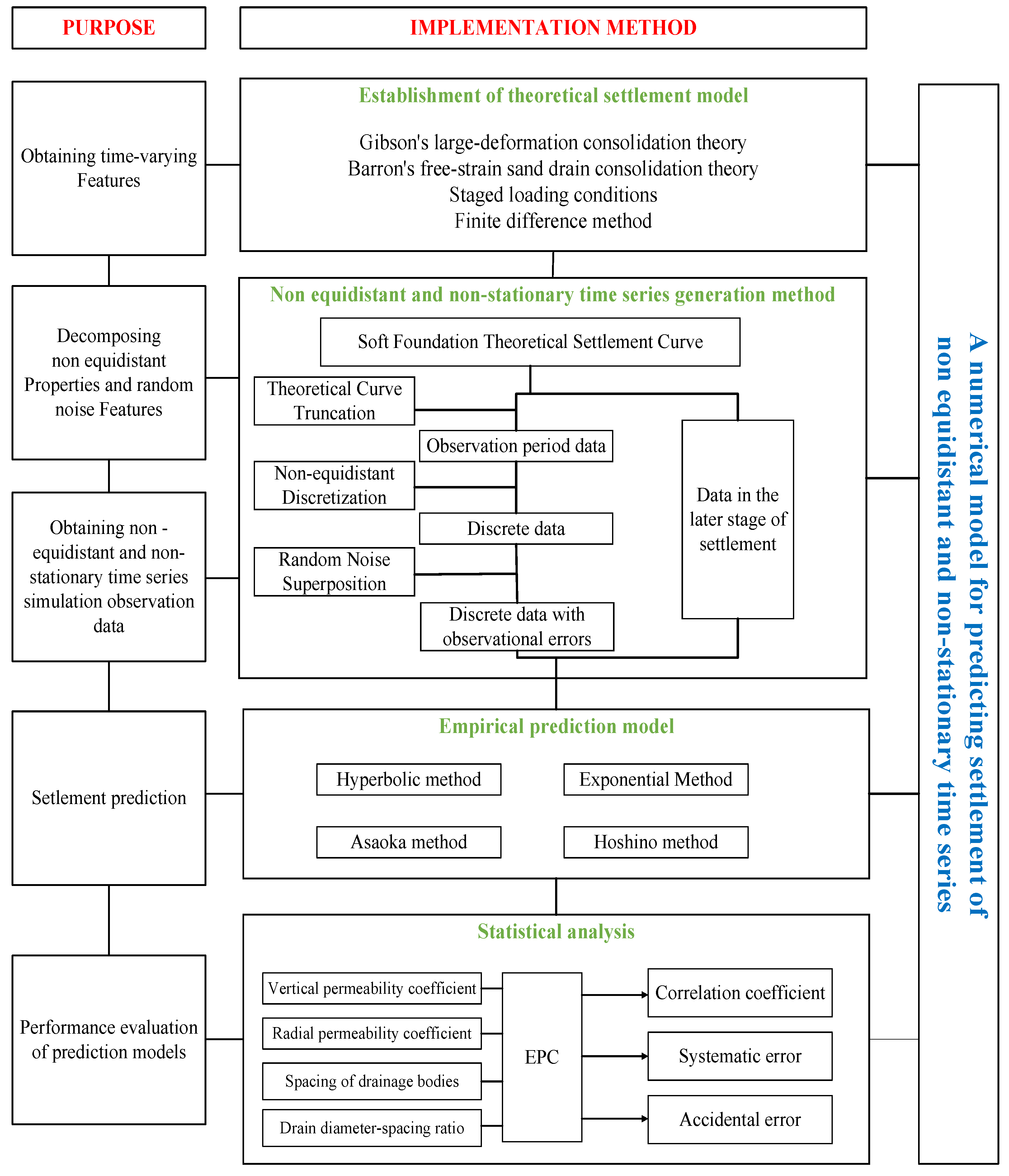
This study employed a technical approach that combines theoretical modeling and numerical simulation to systematically construct an analytical framework for high-speed railway (HSR) soft foundation settlement prediction. The technical workflow is illustrated in Figure 1.
First, a settlement theoretical model was established. This model was based on Gibson’s large-deformation consolidation theory and Barron’s free-strain sand drain consolidation theory and incorporated staged loading conditions. By rigorously controlling key parameters (such as vertical permeability coefficient, radial permeability coefficient, and drain diameter–spacing ratio), the model could precisely characterize the time-varying settlement features. Validation against field monitoring data confirmed that the computational accuracy of the model met the engineering requirements (with a relative error < 2%).
Second, to tackle the challenges posed by the NENSTS observation data, an innovative data generation method based on Monte Carlo simulation was proposed. This method utilized a three-step processing flow: (i) theoretical curve truncation, (ii) non-equidistant discretization, and (iii) random noise superposition (see details in Section 2.1.2). This approach allowed for the quantitative separation of time-varying features from random noise features and simultaneously generated large-scale, engineering-relevant data samples (with a magnitude of 104 per simulation).
Finally, four typical empirical models (Hyperbolic, Exponential, Asaoka, and Hoshino) were evaluated using a controlled variable approach. By normalizing the consolidation characteristics of surcharge-preloaded sand drain soft foundations through the EPC method, repeated prediction experiments (n = 1040 times) were designed to quantify key indices, including the correlation coefficient, systematic error, and random error. This generated a robust dataset for subsequent multi-index evaluation.

2.1.1. Establishment of Settlement Theoretical Model

Based on Gibson’s large-strain consolidation theory and Barron’s free-strain sand drain consolidation theory, a theoretical settlement model for soft foundations incorporating staged loading was developed. The core assumptions of the model incorporate fully saturated soil with incompressible solid particles and pore water, negligible lateral deformation (excluding well resistance and smear effects), and permeable top boundary with impermeable bottom/radial outer boundaries.
The governing equations of the model are given in Appendix A, Equation (A11), and detailed derivations, boundary conditions, and solution procedures are also provided in Appendix A.

2.1.2. Method for Generating NENSTS

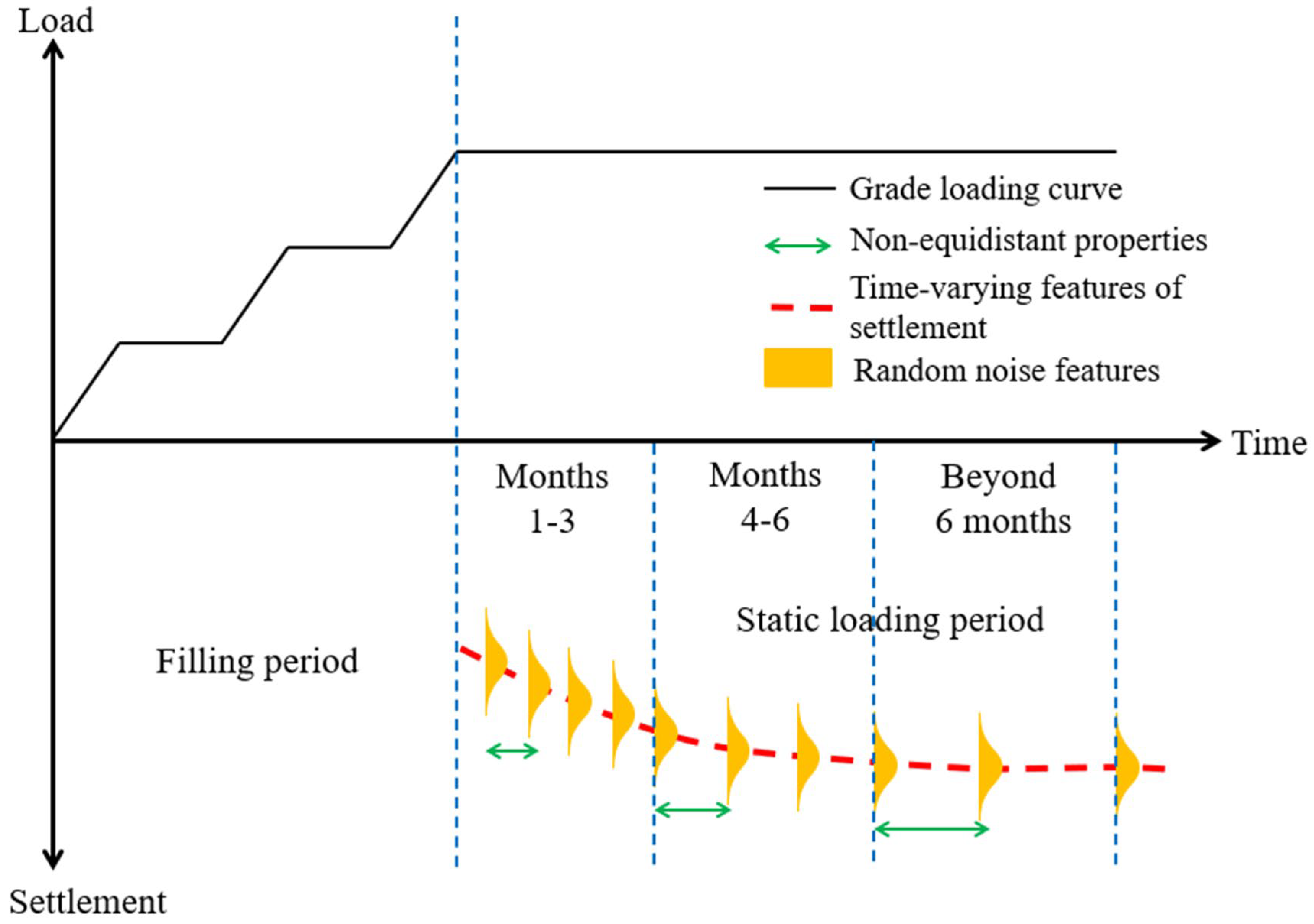
A framework based on Monte Carlo simulation was developed to generate the NENSTS observation data (Figure 2). This framework can quantitatively decouple and control three key features of observational data: non-equidistant properties, time-varying features, and Gaussian-distributed random noise features (Appendix B). The detailed steps are as follows:
Step 1. Theoretical Data Computation
The settlement theoretical model described in Section 2.1.1 was used to calculate time-dependent settlement curves with controlled consolidation parameters.
Step 2. Theoretical Curve Truncation
The complete settlement curve was divided into observation period data and post-settlement period data by means of theoretical curve truncation (Appendix B, Figure A4a).
Step 3. Non-Equidistant Discretization
Observation period data were discretized by applying the non-equidistant discretization method (Appendix B, Figure A4b).
Step 4. Random Noise Superposition
Gaussian random noise was superimposed onto the discretized data through random noise superposition (Appendix B, Figure A4c). This process simulates the generation of the NENSTS observation data.
Step 5. Large-Scale Repeated Settlement Prediction
Four empirical models, namely, Hyperbolic, Exponential, Asaoka, and Hoshino models [27,28,29,30], were iteratively applied to the synthesized non-equidistant and non-stationary data for repeated settlement predictions. This enabled a systematic evaluation of model robustness (Appendix B, Figure A4d).

2.1.3. Solution Strategy and Result Statistical Methods

Objective Function of Prediction Models
The fitting parameters of four empirical prediction models were determined by the least squares method. The objective function, based on the least squares principle [31] (see Equation (1), as shown in Figure 3), is:
arg min Y = i = 1 N ( y i y ^ i ) 2
where N represents the number of simulated observational data points, y i represents the true value, which is directly obtained from the simulated data, and y ^ i represents the fitted value, and each empirical model processed it differently.
Normalization of Permeability for Surcharge-Preloaded Soft Foundations
In this study, the equivalent permeability coefficient (EPC) proposed by Chai [32] (Equations (2) and (3)) was used to normalize the factors that affect the consolidation characteristics of surcharge-preloaded sand drain soft foundations:
K v e = 1 + 2.5 × l 2 F n × D e 2 × K ζ K r · K ζ
F n = n 2 n 2 1 × ln ( n ) 3 · n 2 1 4 · n 2
where K v e is the equivalent permeability coefficient (EPC), l is the installation depth of the drainage body ( l = H in this study), and n is the drain diameter–spacing ratio ( n = D e / r d ).
Statistical Analysis of Prediction Results
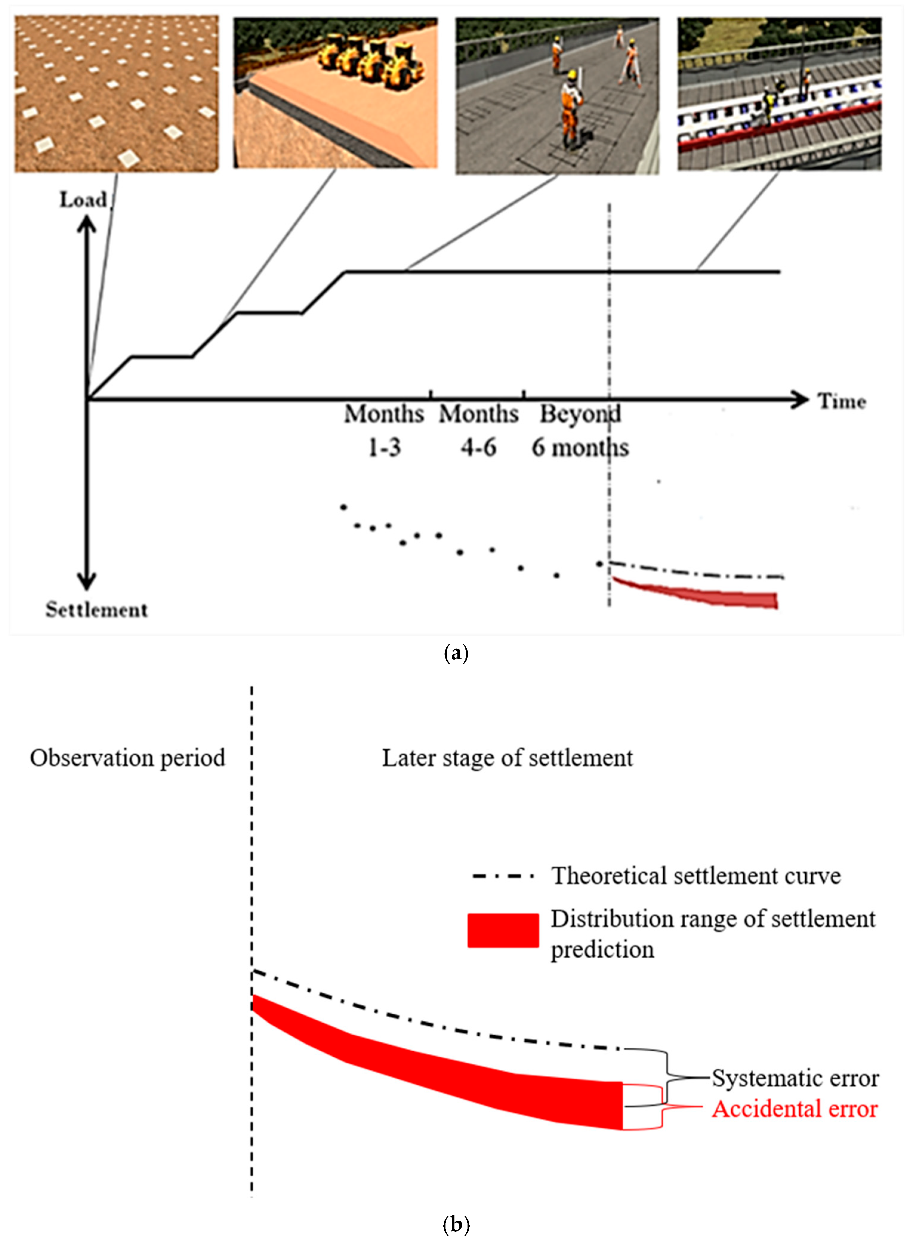
The correlation coefficient [5,6] is a commonly used statistical indicator. As depicted in Figure 4a,b, statistical analysis was conducted on the repeated settlement prediction results. The deviation between the mean final settlement [33] (Equation (5)) and the theoretical settlement curve is defined as the systematic error of the empirical model, as described in Equations (6) and (7). The fluctuation range, quantified by the standard deviation, of the final settlement represents the random error [33], as shown in Equation (8):
r = C o v ( X ¯ , Y ¯ ) D ( X ¯ ) · D ( Y ¯ )
μ = 1 N s k = 1 N s S k
A E = μ S
R E = A E / S
S D = 1 N s 1 k = 1 N s [ S k μ ] 2
where r represents the correlation coefficient, μ represents the predicted mean value, A E represents the predicted absolute error, R E represents the predicted relative error, S represents the theoretical final settlement, S D represents the predicted standard deviation, N s represents the number of observational samples per trial, and S k represents the k -th prediction value.

2.2. Verification of the Predictive Numerical Analysis Model

2.2.1. Reliability Verification of the Settlement Theoretical Model

Hu et al. [34] carried out field monitoring on marine sedimentary soft foundations in Shenzhen, where plastic drainage boards were employed for foundation treatment (Table 1). The theoretical model was utilized to calculate the time-dependent settlement curve of this site, and the calculation results were compared with the monitoring data (Figure 5). The time-varying characteristics of the theoretical settlement calculations are consistent with the trends of field monitoring. When the static loading duration reached 400 days, the theoretical settlement was 224 cm, while the field measurement result was 228 cm, resulting in a relative error of only 1.75%. This result validates the reliability of the theoretical model.

2.2.2. Convergence Testing of Monte Carlo Simulation

The sample size has an impact on the accuracy of Monte Carlo simulations. To verify the convergence of the numerical model and determine the minimum sample size that can meet the precision requirements, a convergence test was conducted by using the case of Hu et al. [33].
During the static phase (starting from the 210th day of construction), data were sampled once a week for the first three months and once every two weeks for months four to six. The observation period lasted for 6 months, with a total of 21 observations. The measurement accuracy conformed to Class III standards (see Table 3). The single-sample size ranged from 10 to 300, resulting in a total sample size of 210 to 9600. Predictions based on 1 × 10⁷ samples (with a total of 2.1 × 10⁸) were used as the benchmark for the convergence testing of the mean and standard deviation.
(1)
Settlement Prediction Mean Convergence
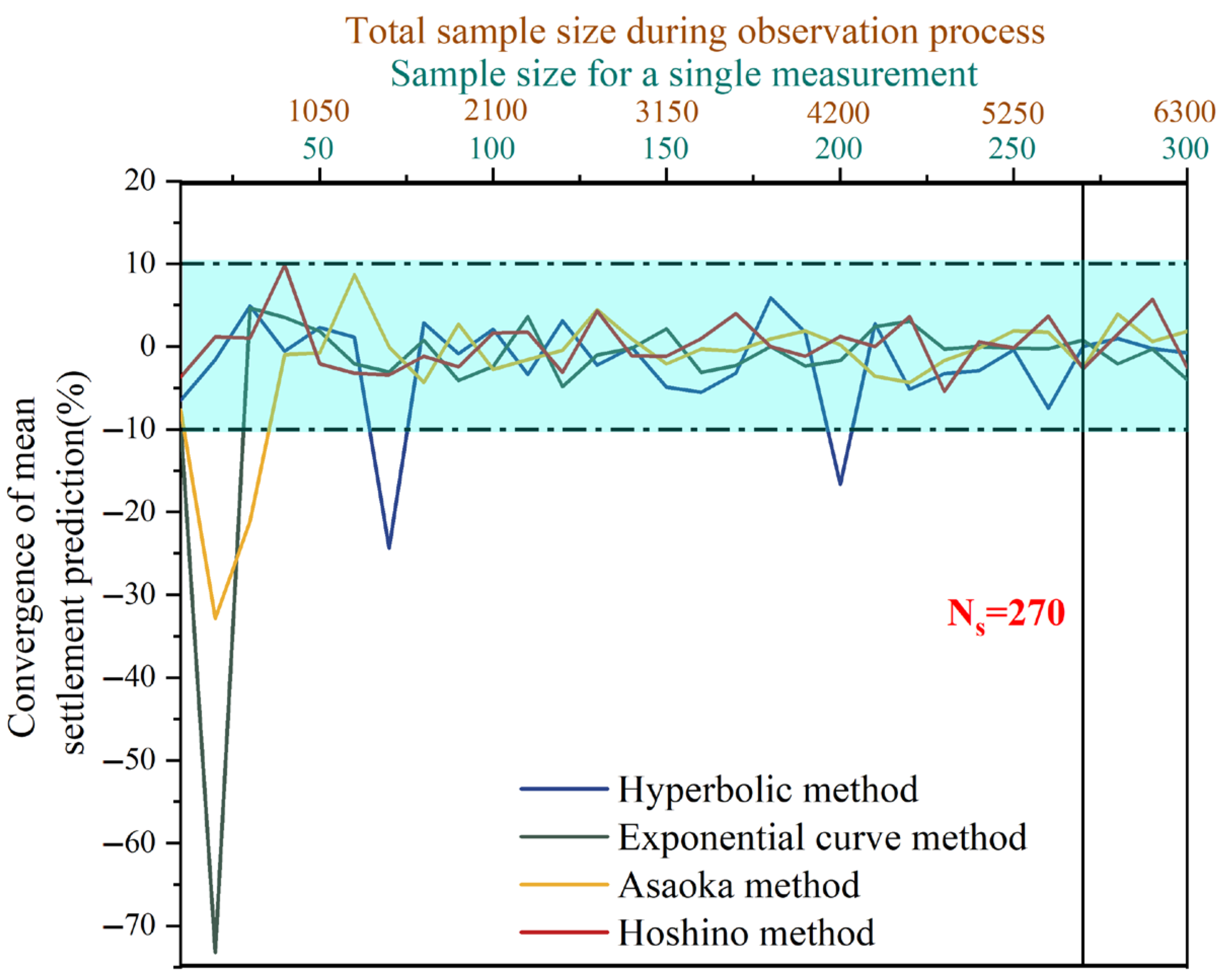
As illustrated in Figure 6, when the deviation threshold was set at 10% [34], the Exponential and Asaoka methods showed significant mean fluctuations under low sample sizes ( N s < 270). However, an increase in the sample size reduced the variability. In contrast, the Hyperbolic and Hoshino methods exhibited smaller mean fluctuations. For N s ≥ 270, all models achieved stable mean predictions.
(2)
Settlement Prediction Standard Deviation Convergence
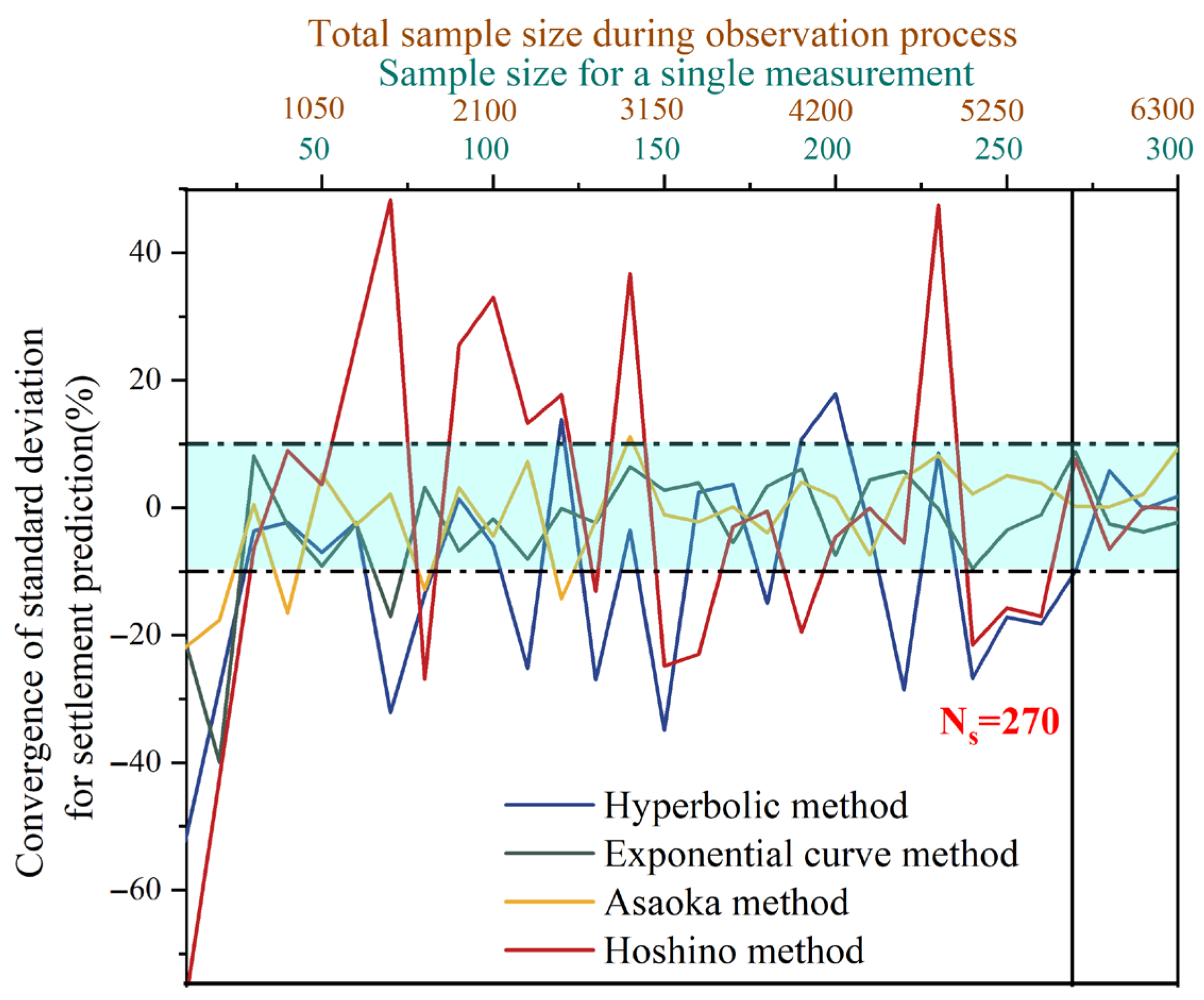
As depicted in Figure 7, with the same 10% deviation threshold, the Hyperbolic, Exponential, and Hoshino methods showed larger standard deviation fluctuations at low sample sizes, whereas the Asaoka method remained relatively stable. For N s ≥ 270, all models achieved the control of standard deviation variability.

2.3. Parameterization of the Predictive Numerical Analysis Model

2.3.1. Parameter Selection for the Settlement Theoretical Model

(1)
Soil Property Parameters
The vertical permeability coefficient of soft soils differs with their genesis, and typical empirical values range from 1 × 10⁻⁴ to 1 × 10⁻³ m/d [35]. In this study, values of 2.76 × 10⁻⁴ to 1.36 × 10⁻³ m/d were selected for the vertical permeability coefficient.
In soft foundations, radial permeability generally exceeds vertical permeability. Leroueil [36] experimentally obtained anisotropy ratios of 1.35–1.55 for Louiseville clay, Adams [37] reported ratios of 1.2–1.9 for Boston blue clay, and Basak [38] determined ratios of 1.0–1.6 for remolded kaolin. Based on these results, anisotropy ratios of 1.1–1.9 were selected. Key soil parameters are listed in Table 2.
(2)
Loading Conditions
The critical filling height of soft foundations was determined by the Fellenius method [40] (Equation (9)):
γ w · ρ · H c r i t = 5.52 · C u
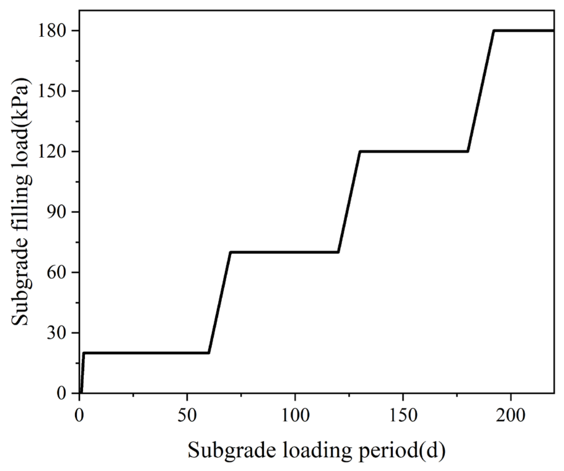
where ρ represents the density of soft soil, H c r i t represents the critical filling height, calculated as 9 m (final load: 180 kPa), and C u represents the vane shear strength. Taking the surface sand cushion layer into account (initial load: 20 kPa), the staged loading conditions are shown in Figure 8.

2.3.2. Observational Condition Parameters

(1)
Measurement Accuracy
Deformation observations of railway subgrades comply with Class III standards [5,6]. Random errors were modeled as a normal distribution, with precision requirements detailed in Table 3 [41].
(2)
Observation Frequency and Duration
Observation frequencies conformed to specifications [5,6] (Table 4). The observation and evaluation period was 12 months. Data in the later stage of settlement—used to analyze and comparatively validate the accuracy and stability of settlement predictions—spanned 5 years, during which the settlement rate was maintained below 1.0 × 10⁻⁵ m/d.

3. Results and Discussion

3.1. Variation Patterns of Evaluation Index for Empirical Prediction Models

3.1.1. Correlation Coefficient Variation Patterns

The correlation coefficient (Equation (4)) served as an index for characterizing the time-varying features of settlement curves.
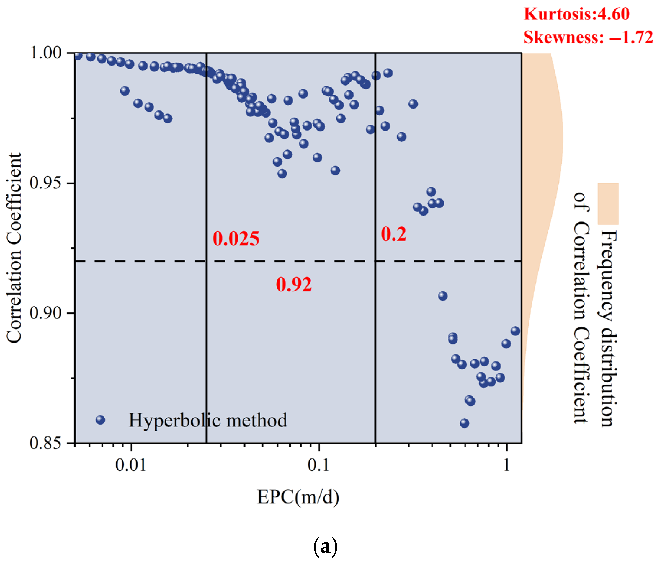
For the Hyperbolic method (Figure 9a), when the equivalent permeability coefficient (EPC) < 0.2 m/d, the correlation coefficient exceeded 0.92, within 0.025–0.2 m/d, the correlation coefficient showed moderate fluctuations, and when EPC > 0.2 m/d, the correlation coefficient decreased rapidly with increasing EPC and dropped below 0.92. This indicates that the goodness-of-fit of the Hyperbolic method weakened gradually as EPC increased.
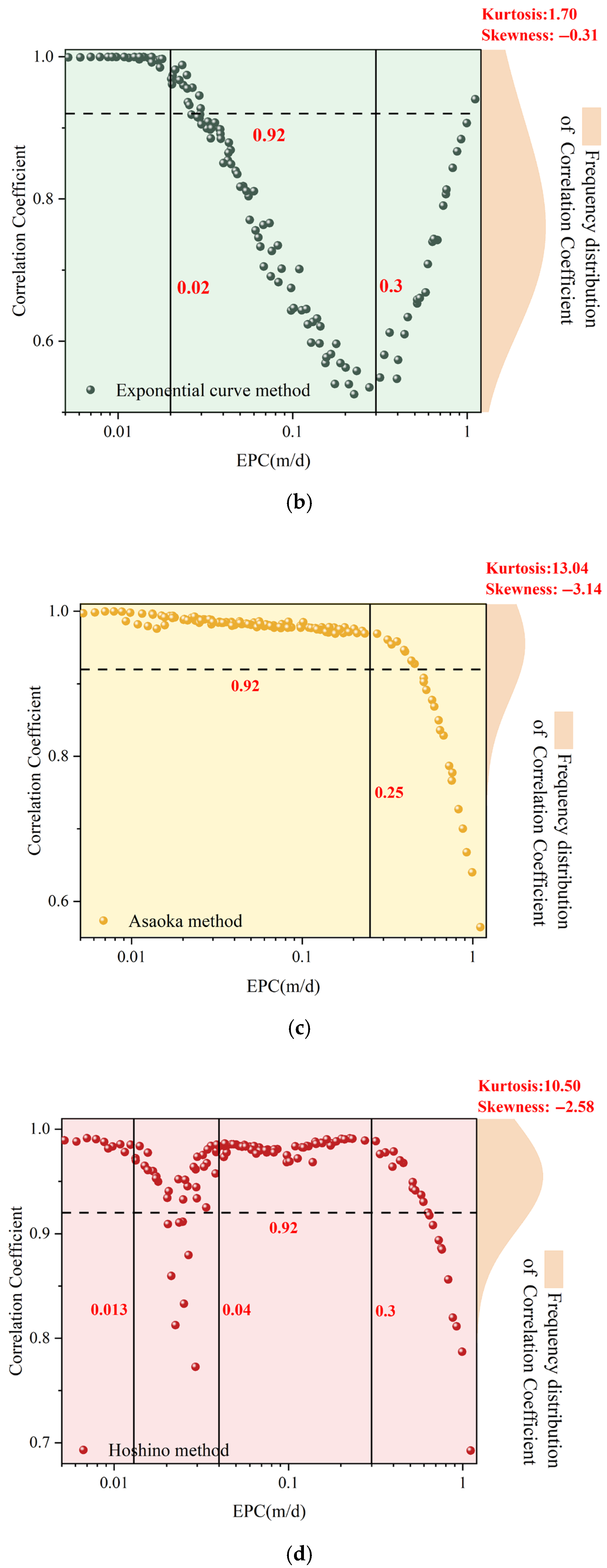
For the Exponential method (Figure 9b), when EPC < 0.02 m/d, the correlation coefficient was ≥0.92, when EPC ≥ 0.02 m/d, the correlation coefficient was <0.92, within 0.02–0.3 m/d, the correlation coefficient decreased with increasing EPC, and when EPC > 0.3 m/d, the correlation coefficient increased with EPC. This demonstrates that the goodness-of-fit of the Exponential method first weakened and then strengthened as EPC increased.
For the Asaoka method (Figure 9c), when EPC < 0.25 m/d, the correlation coefficient was ≥0.92, and when EPC > 0.25 m/d, the correlation coefficient decreased with increasing EPC and dropped below 0.92. This reveals that the goodness-of-fit of the Asaoka method weakened gradually as EPC increased.
For the Hoshino method (Figure 9d), when EPC < 0.012 m/d or within 0.015–0.3 m/d, the correlation coefficient was ≥0.92, within 0.013–0.04 m/d, the correlation coefficient exhibited fluctuations (even dropping below 0.92), and when EPC > 0.03 m/d, the correlation coefficient decreased with increasing EPC and dropped below 0.92. This indicates that the goodness-of-fit of the Hoshino method generally weakened with increasing EPC, accompanied by localized fluctuations and oscillations.
Further analysis of Figure 9a–d revealed the following: the Hyperbolic method—kurtosis = 4.60 and skewness = −1.72, the Exponential method—kurtosis = 1.70 and skewness = −0.31, the Asaoka method—kurtosis = 13.04 and skewness = −3.14, and the Hoshino method—kurtosis = 10.50 and skewness = −2.58.

3.1.2. Systematic Error Variation Patterns

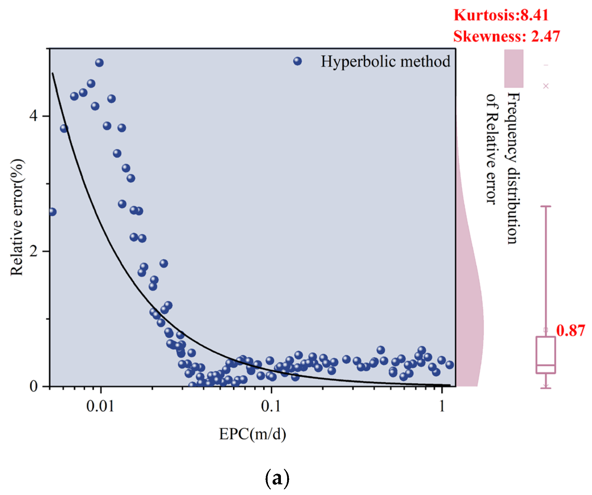
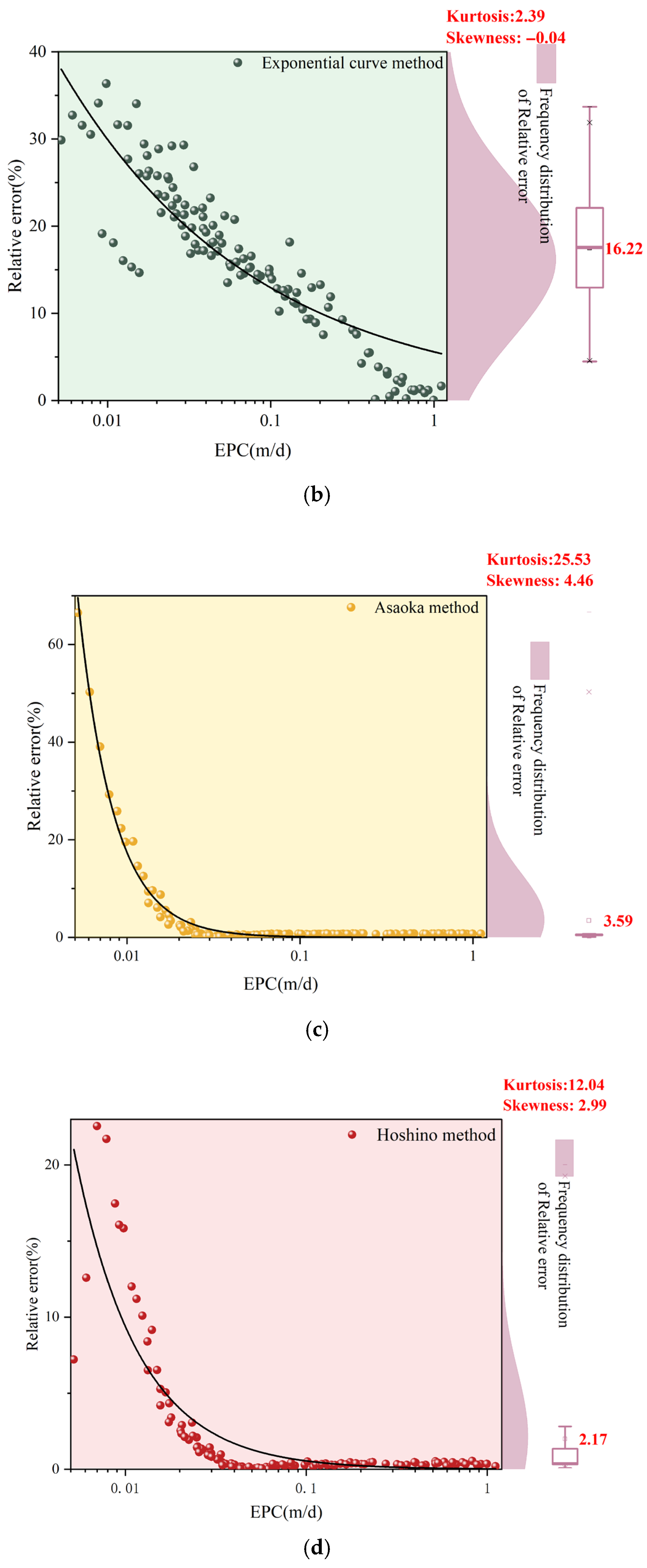
The relative error (Equation (7)) served as an index to characterize the systematic error in settlement predictions. As depicted in Figure 10a–d, systematic errors exhibited a power-law decay trend ( R E K v e P ) with increasing EPC. This was primarily attributed to the accelerated consolidation rates in high-permeability soils. The reduction in systematic error arose because, under the same observation duration, frequency, and accuracy, soft foundations with higher EPC showed greater settlement completion rates. Consequently, the time-varying characteristics of observed data became smoother, and the discrepancy between the predicted final settlement and the settlement at the prediction time decreased. This reduced fitting difficulty and improved prediction accuracy. This conclusion is consistent with the statistical results reported by Kliesch K. [20].
There were differences in the magnitudes of systematic errors among the four models. The Hyperbolic method exhibited a mean systematic error of 0.87%, the Exponential method 16.41%, the Asaoka method 3.59%, and the Hoshino method 2.17%. Ranking the systematic errors in descending order gave: Exponential method > Asaoka method > Hoshino method > Hyperbolic method. This indicates that the Hyperbolic method achieved the highest prediction accuracy, the Exponential method the lowest, and the Asaoka and Hoshino methods exhibited moderate performance.
Statistical analysis of the systematic error distributions yielded the following parameters: the Hyperbolic method—kurtosis = 8.41 and skewness = 2.47, the Exponential method—kurtosis = 2.39 and skewness = −0.04, the Asaoka method—kurtosis = 25.53 and skewness = 4.46, and the Hoshino method—kurtosis = 12.04 and skewness = 2.99.

3.1.3. Random Error Variation Patterns

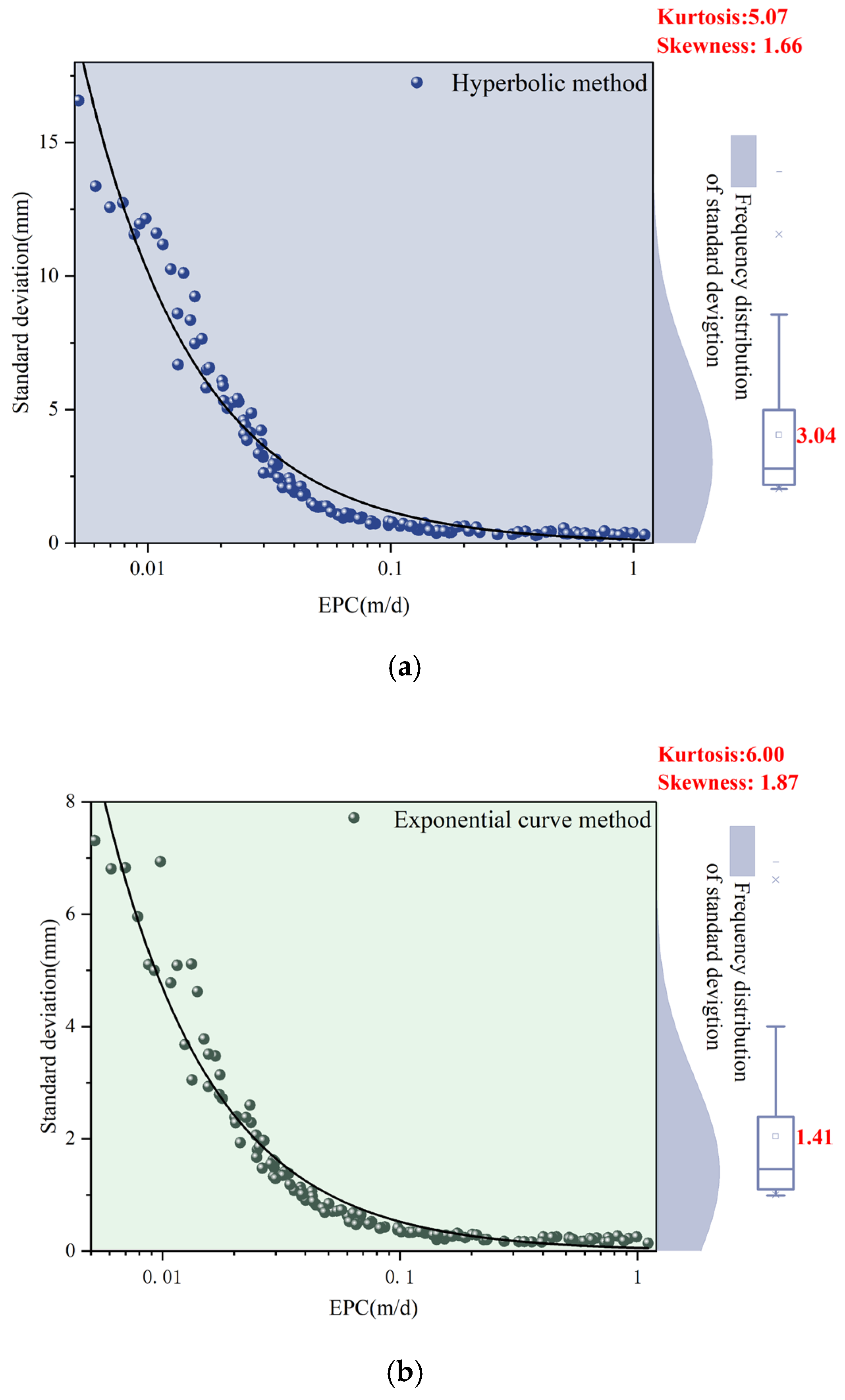
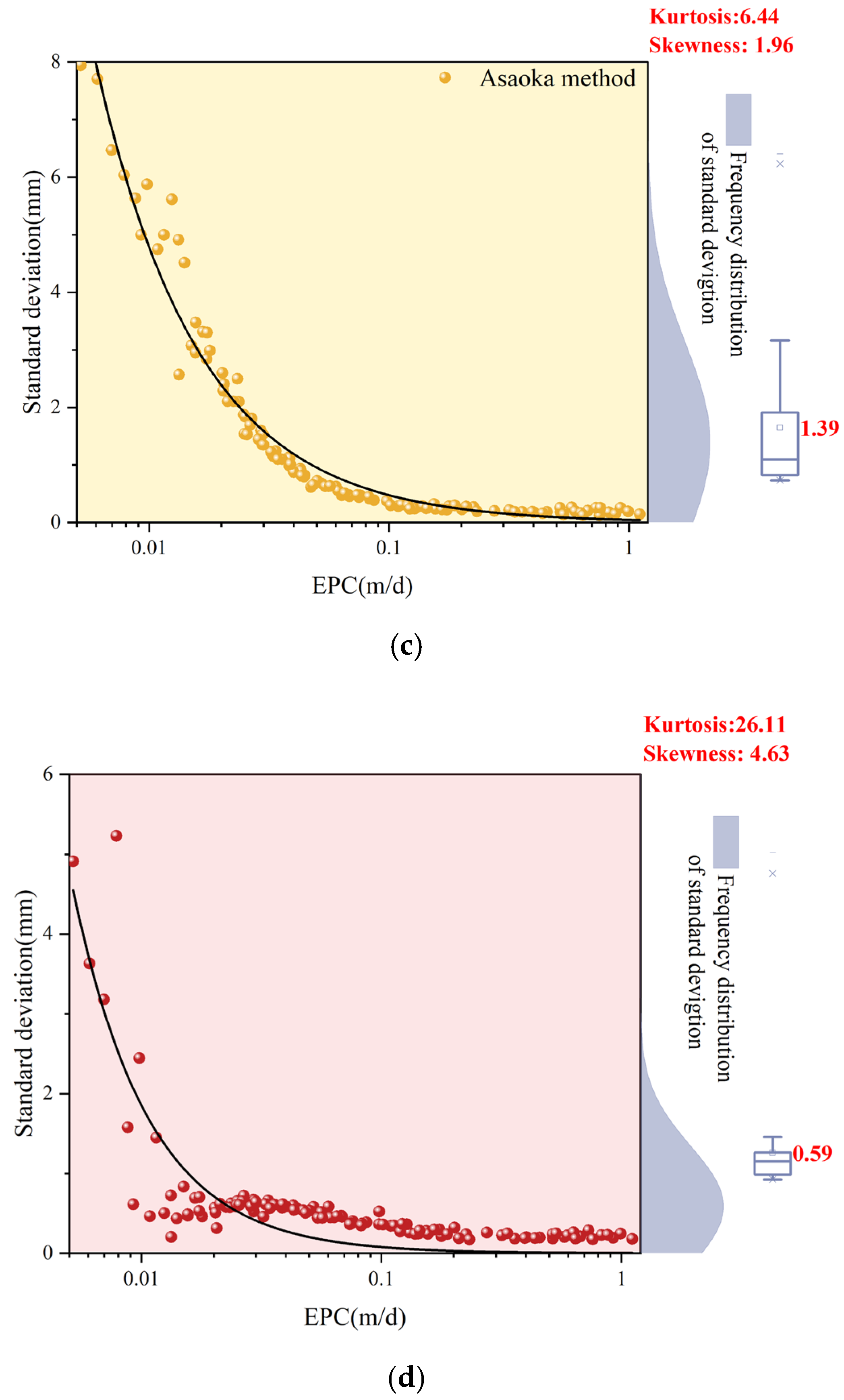
The prediction standard deviation (Equation (8)) was employed as an index to characterize the random error of settlement predictions. As depicted in Figure 11a–d, as the equivalent permeability coefficient (EPC) increased, the random errors displayed a power-law decay trend ( S D K v e P ). This phenomenon was mainly attributed to the accelerated consolidation rates in high-permeability soils. The reduction in random errors occurred because larger EPC values mitigated the coupling effects between non-equidistant and non-stationary properties, thus enhancing the stability of settlement predictions.
The magnitudes of random errors varied significantly across different models. The Hyperbolic method had a mean random error of 3.04 mm, the Exponential method 1.41 mm, the Asaoka method 1.39 mm, and the Hoshino method 0.59 mm. When ranking the random errors in descending order, the result was: Hyperbolic method > Exponential method ≈ Asaoka method > Hoshino method. This suggests that the Hoshino method demonstrated the highest prediction stability, the Hyperbolic method showed the lowest, and the Exponential and Asaoka methods presented intermediate performance.
Statistical analysis of the random error distributions yielded the following parameters: the Hyperbolic method—kurtosis = 5.07 and skewness = 1.66, the Exponential method—kurtosis = 6.00 and skewness = 1.87, the Asaoka method—kurtosis = 6.44 and skewness = 1.96, and the Hoshino method—kurtosis = 26.11 and skewness = 4.63.
A comprehensive analysis revealed the following: The Hyperbolic method had a strong fitting ability for the time-varying characteristics of soft foundation settlement curves. It featured high accuracy but poor stability. The Exponential method could only adequately depict the time-varying characteristics of soft foundations with low permeability and large sand drain spacing. It showed relatively low accuracy but better stability. Both the Asaoka method and the Hoshino method were unsuitable for describing the time-varying characteristics of soft foundations with high permeability and small sand drain spacing. However, they both maintained certain accuracy and stability levels, with the Hoshino method showing the best stability.

3.2. Optimal Application Range Maps of Empirical Models

3.2.1. Determination of Comprehensive Evaluation Index (CEI)

For the observation and evaluation of HSR subgrade deformation, empirical prediction models are required to meet three simultaneous requirements. First, the model should be able to effectively describe the time-varying characteristics of settlement curves with a high goodness-of-fit. Second, for HSR tracks, particularly the newly constructed 400 km/h ballastless tracks, the post-construction settlement limit of subgrades should not exceed 15 mm [42,43], which necessitates high prediction accuracy. Third, the model must show strong stability when processing the NENSTS observation data. This indicates that the performance evaluation of settlement prediction models is a typical multi-objective decision-making process.
The entropy weight method (EWM) is one of the main methods for multi-objective decision-making [44]. The weights obtained by EWM reflect the dispersion degree of each index. It has advantages, such as simple calculation, mathematical rigor, and the avoidance of subjective bias in weight assignment [45]. Nevertheless, the traditional EWM is highly sensitive to skewed distributions and outliers, which directly weakens the robustness of the determined weights. Skewness–kurtosis tests [46,47] on the tri-variate distributions of correlation coefficients, systematic errors, and random errors (Figure 9a–d, Figure 10a–d and Figure 11a–d) showed that the absolute skewness values of most results exceeded 1.0, and the kurtosis exceeded 5.0. This indicates skewness and the presence of outliers in the data. To solve this problem, a robust entropy weight method (REWM) that incorporates robust statistical processing was proposed to construct the CEI.
To overcome the limitations of the traditional EWM in processing data with large fluctuations under the NENSTS conditions, this study proposed an improved entropy weight method. The proposed method replaces conventional statistical parameters (mean and standard deviation) with robust statistical parameters (median and interquartile range) for calculating index weights, thus improving the stability of weight determination. The specific steps are as follows:
Step 1. Identify and handle outliers using the interquartile range (IQR) method.
Calculate the first quartile ( Q 1 ) and third quartile ( Q 3 ) of each evaluation index, namely, the correlation coefficient, systematic error, and random error, for the four empirical models. Determine the upper and lower bounds for outliers and replace values outside this range with the corresponding boundary values:
x L o w e r = Q 1 1.5 × I Q R x u p p e r = Q 3 + 1.5 × I Q R
where I Q R = Q 3 Q 1 .
Step 2. Construct the judgment matrix A:
A = ( x i j ) , ( i = 1 , 2 , , q ; j = 1 , 2 , , p )
Step 3. Conduct quantile-based Winsorization, followed by standardization, to obtain the standardized judgment matrix B:
B = ( b i j ) = x i j x l o w e r , j x u p p e r , j x l o w e r , j ( i = 1 , 2 , , q ; j = 1 , 2 , , p )
where x l o w e r , j and x u p p e r , j represent the lower bound and upper bound of different entities under the same index, respectively.
Step 4. Based on the definition of entropy, for the four entities and three evaluation indices, the entropy of each evaluation index can be determined as follows:
H i = 1 ln p j = 1 p ( f i j · ln f i j ) , ( i = 1 , 2 , , q ; j = 1 , 2 , , p )
f i j = b i j j = 1 p b i j
Step 5. Calculate the entropy weights of the evaluation indices:
W = ( ω i ) 1 × q
ω i = 1 H i q i = 1 q H i   and   i = 1 q ω i = 1
After robust statistical processing, the CEI is expressed by Equation (17):
Ω = 0.33 × r n + 0.33 × ( 1 R E n ) + 0.34 × ( 1 S D n )
where Ω represents the comprehensive evaluation index (CEI), while r n , R E n , and S D n denote the standardized correlation coefficient, systematic error, and random error, respectively.

3.2.2. Determination of Optimal Application Scope

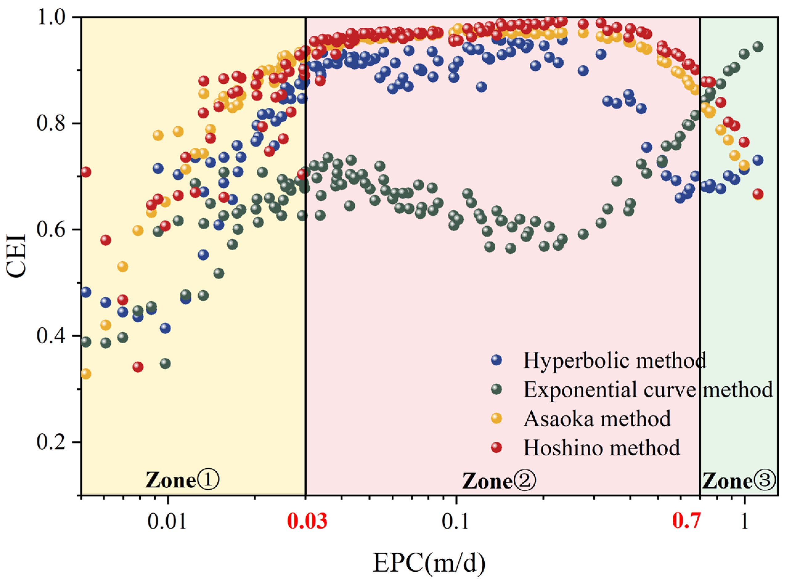
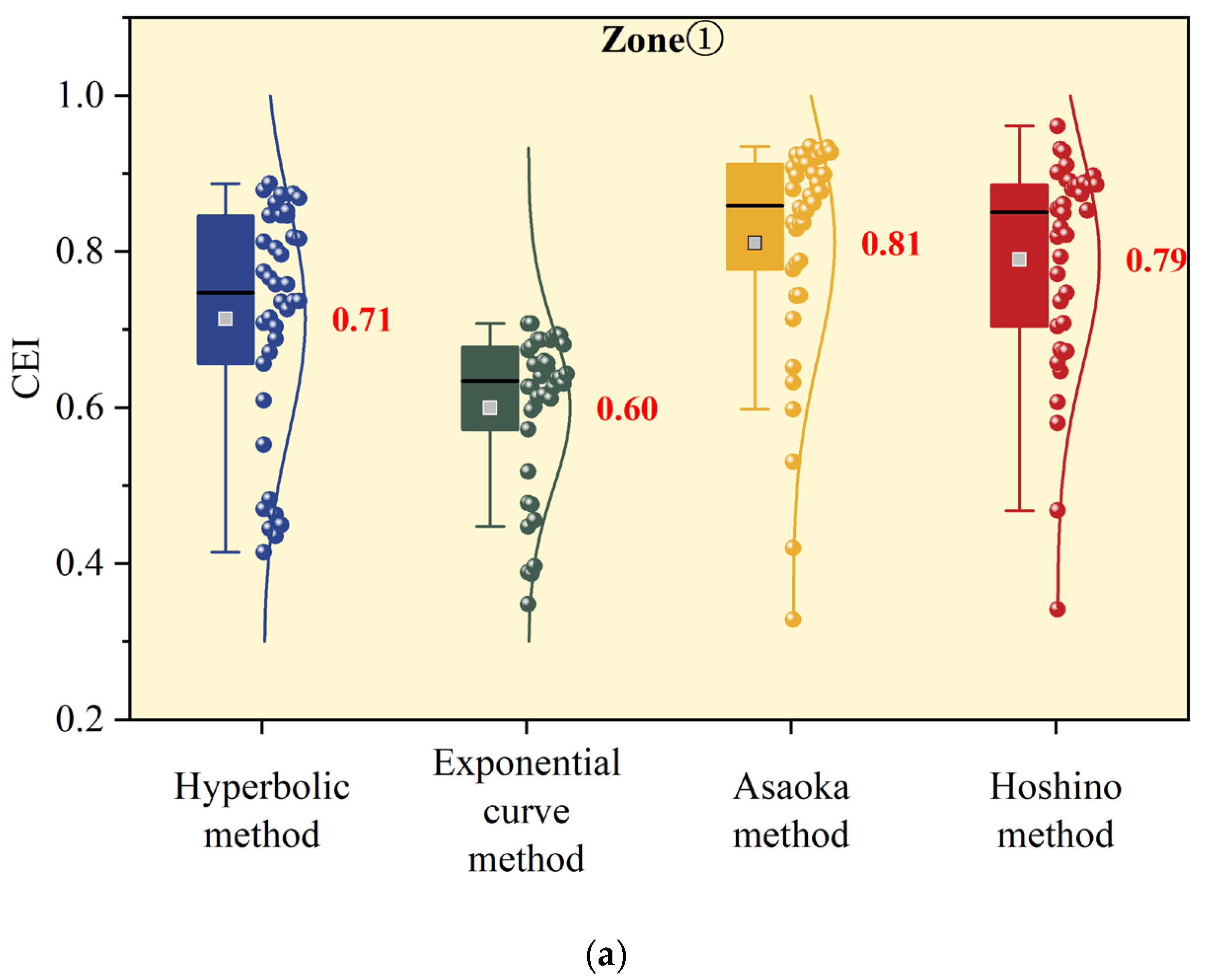
As depicted in Figure 12, the CEI derived from the four empirical models displayed different trends as the EPC changed. Additionally, a preliminary comparison among the models is presented. When the EPC was less than 0.03 m/d, the CEI values of all four models showed overall poor performance and increased as the EPC increased. This range is proposed to be classified as Zone ①. In the range of 0.03–0.7 m/d, the Hyperbolic, Asaoka, and Hoshino methods showed relatively stable performance, whereas the Exponential method performed poorly. This range is proposed to be classified as Zone ②. When the EPC was greater than 0.7 m/d, the CEI values of the Hyperbolic, Asaoka, and Hoshino methods decreased as the EPC increased, while the Exponential method showed enhanced performance. This range is proposed to be classified as Zone ③.
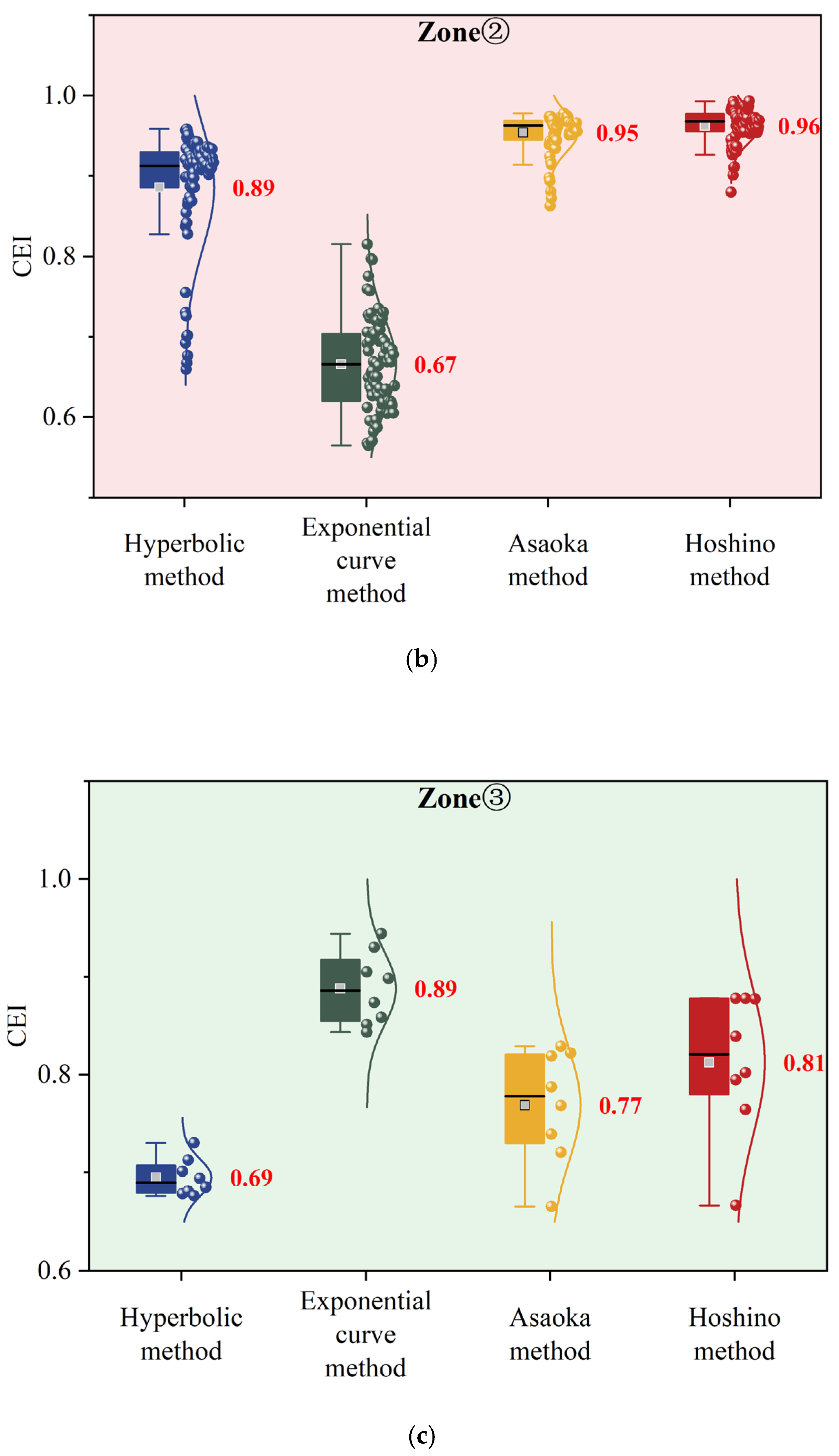
Specifically, as depicted in Figure 13a, when EPC ≤ 0.03 m/d, the average CEI values of the four methods were 0.71, 0.60, 0.81, and 0.79, respectively. The ranking of the mean values was: Asaoka method > Hoshino method > Hyperbolic method > Exponential method. The standard deviations were 0.15, 0.13, 0.14, and 0.14, which indicates that the dispersion differences among the models were low. Thus, within Zone ①, the Asaoka method was the optimal choice. Within the range of 0.03–0.7 m/d, as shown in Figure 13b, the average CEI values of the models were 0.89, 0.67, 0.95, and 0.96, respectively. The standard deviations were 0.08, 0.06, 0.05, and 0.05, and the dispersion ranking was: Hoshino method ≈ Asaoka method < Exponential method < Hyperbolic method. Therefore, within Zone ②, the Hoshino method was the optimal choice. When EPC > 0.7 m/d, as shown in Figure 13c, the average CEI values of the models were 0.69, 0.89, 0.77, and 0.81, respectively. The ranking of the mean values was: Exponential method > Hoshino method > Asaoka method > Hyperbolic method. The standard deviations were 0.02, 0.03, 0.06, and 0.07, and the dispersion ranking was: Hyperbolic method < Exponential method ≈ Hoshino method ≈ Asaoka method. Hence, within Zone ③, the Exponential method was the optimal choice.

4. Case Study Validation

4.1. Instance Overview

(1)
Design Key Parameters
Basic profile: A HSR subgrade test section was constructed. It had a length of 65 m and a height of 4.5 m. The entire subgrade had a 1:1.5 slope ratio. Berms, which were 1.0 m high and 1.0 m wide, were constructed at the toe. A ballastless track slab was laid on the subgrade surface.
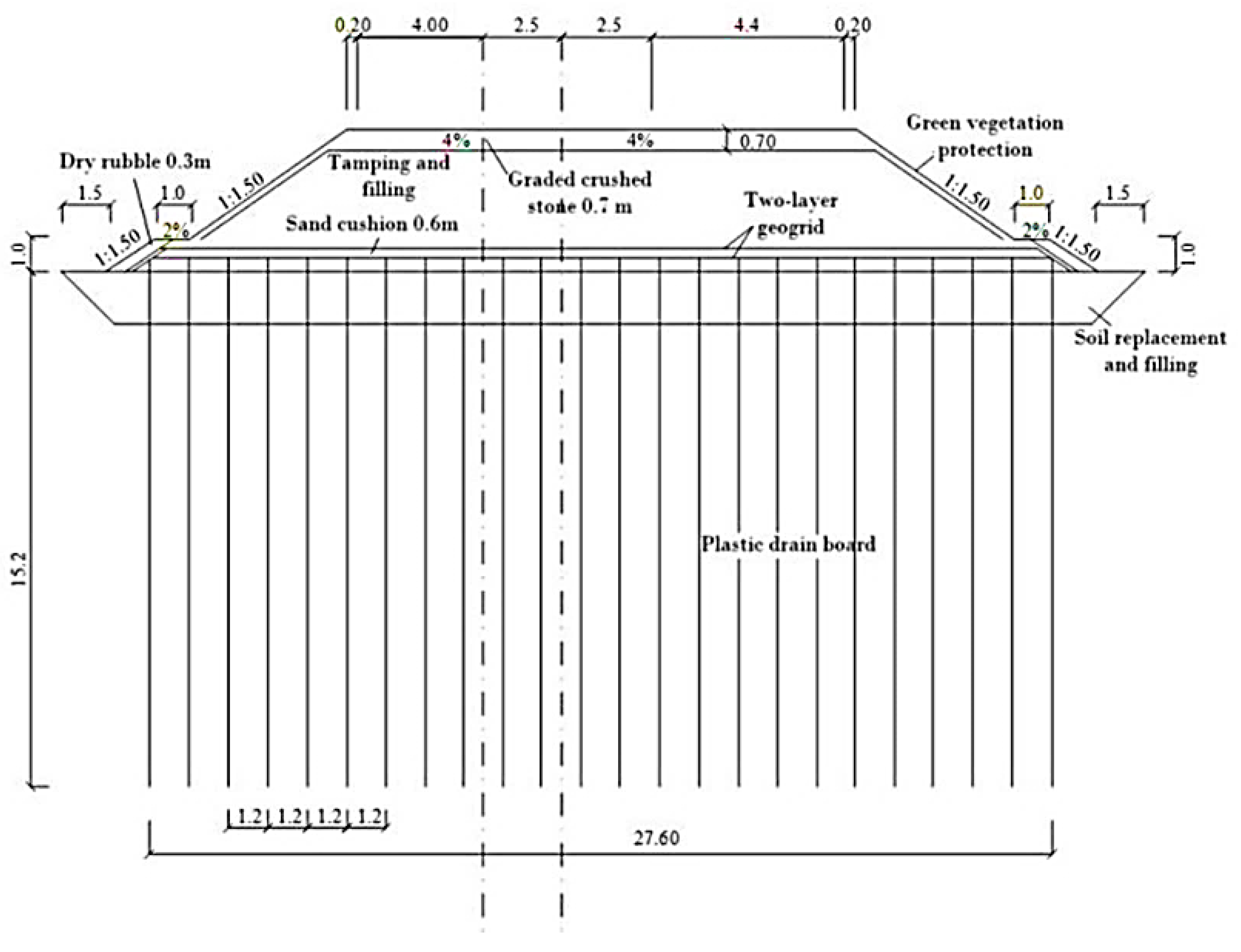
Foundation treatment: Plastic drainage boards were arranged in a triangular pattern with a spacing of 1.2 m and installed to a depth of 15.2 m. A 0.6 m-thick medium-coarse sand cushion layer was placed at the base. To enhance subgrade stability, two geogrid layers, which were spaced 0.2 m apart, were installed at a depth of 0.3 m. The cross-section of the soft foundation treatment is presented in Figure 14.
Construction phasing: The construction period for the sand cushion and subgrade was 293 days. The filling period was 30 days. The static loading period was 325 days, and the construction period for the subgrade surface layer was 39 days.
(2)
Soft Foundation Geotechnical Parameters
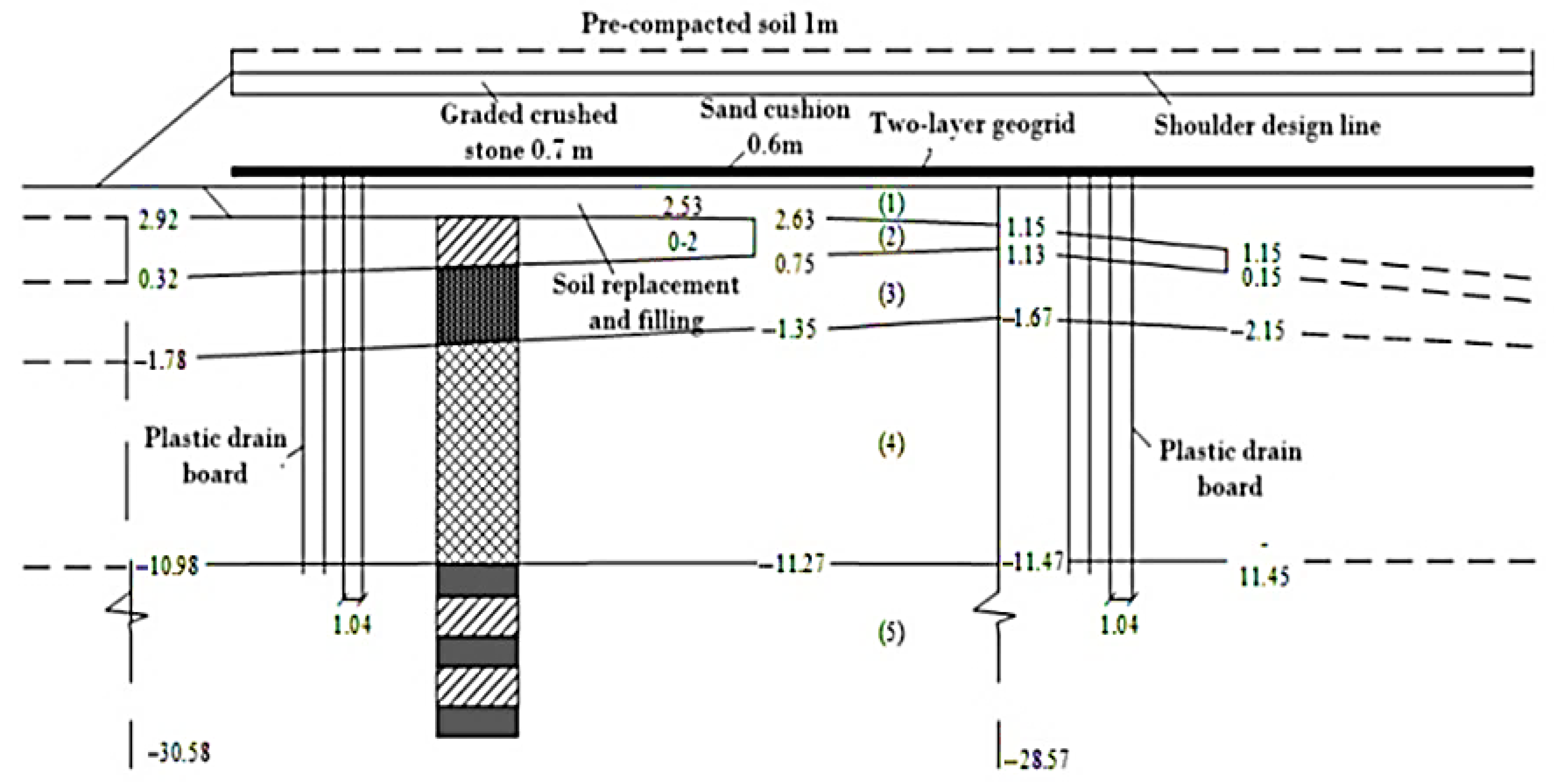
Borehole data revealed the presence of five geotechnical layers within a depth of 15 m. The geological profile is presented in Figure 15. The physical and mechanical properties of each soil layer are summarized in Table 5.
(3)
Deformation Monitoring Conditions and Data
Measurement accuracy: The measurement followed the Class III deformation measurement standards (±1.0 mm; see Table 3).
Observation frequency: During months 1–3 (the static loading period), the observation frequency was once a week. From months 4 to 6, it was once every two weeks. Beyond 6 months, the frequency was once a month. The settlement monitoring curve is presented in Figure 16.

4.2. Selection of Settlement Prediction Model

To generalize the theoretical analysis results derived from homogeneous assumptions to layered soft foundations, the EPCs (excess pore-pressure coefficients) for this scenario were calculated using Equations (2), (3) and (18) [48] via weighted averaging. The EPC of the site was determined to be 0.08 m/d, which falls within the range of 0.03–0.7 m/d. According to the theoretical analysis, the Hoshino method was the optimal choice for this condition:
K ¯ v e = H j = 1 n h j K v e j
where K ¯ v e represents the weighted average equivalent permeability coefficient of the layered soft foundation, K v e j represents the equivalent permeability coefficient of the j-th soil layer, and h j denotes the thickness of the j-th soil layer.

4.3. Validation of Results

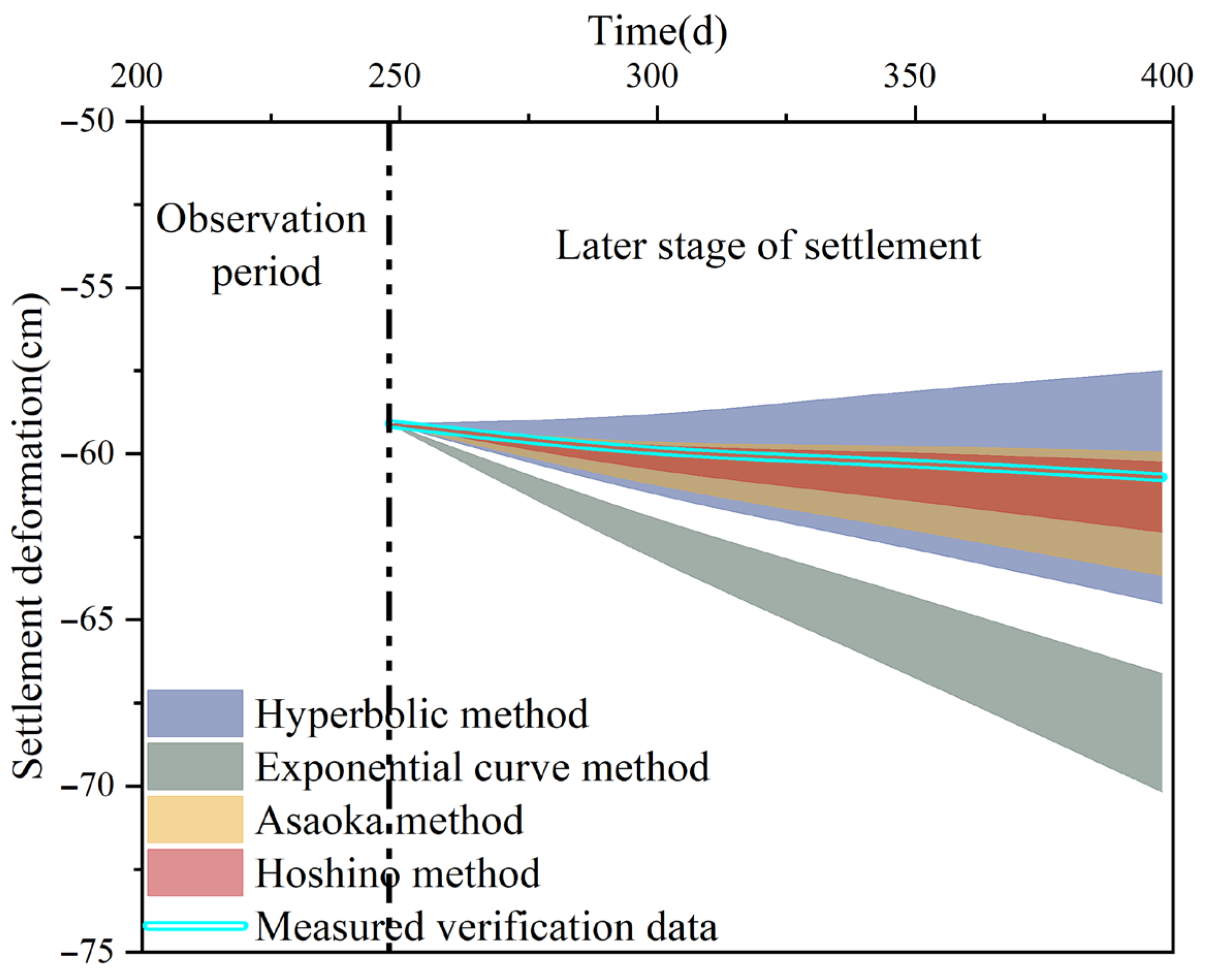
Settlement predictions were performed using these methods, see Figure 17. The correlation coefficients, systematic errors, random errors, and comprehensive evaluation indices are tabulated in Table 6. For this case, the Asaoka method, Hoshino method, and Hyperbolic method achieved correlation coefficients of ≥0.92, which indicated a strong correlation with the settlement curves. In contrast, the Exponential method exhibited poor fitting performance. The Hoshino method and Hyperbolic method demonstrated high prediction accuracy. The Asaoka method ranked third, and the Exponential method showed the poorest performance. The ranking of prediction stability was as follows: Hoshino method > Asaoka method > Exponential method > Hyperbolic method.

5. Conclusions

A predictive framework was established for surcharge-preloaded high-speed railway (HSR) soft foundations. This framework integrated Monte Carlo simulation and equivalent permeability coefficient (EPC) normalization. It proposed a three-step data processing method, namely, “theoretical curve truncation—non-equidistant discretization—random noise superposition”. This method quantified the coupled effects of non-equidistant properties, time-varying features, and random noise features. As a result, it enabled the batch generation of 10,000 simulated samples with controlled spatiotemporal features. Through reliability verification and convergence testing, the computational accuracy of the model was confirmed, with a relative error of less than 2%. This provides a robust tool for probabilistic settlement analysis.
The Hyperbolic method showed a strong goodness-of-fit for the time-varying features of settlement curves and had high prediction accuracy, with a mean systematic error of 0.74%. However, it exhibited poor stability, with a mean standard deviation of 3.04 mm. The Exponential method demonstrated good goodness-of-fit only for soft foundations with low permeability and large sand drain spacing (EPC > 0.3 m/d). It had moderate accuracy but better stability. The Asaoka and Hoshino methods showed poor goodness-of-fit for soft foundations with high permeability and small sand drain spacing. Nevertheless, they maintained reasonable accuracy and stability. Among them, the Hoshino method achieved the best stability, with a mean standard deviation of 0.59 mm.
A multi-index evaluation system based on REWM was developed. This system assigned weights of 33% to goodness-of-fit, 33% to accuracy, and 34% to stability. The derived applicability maps allowed engineers to select the optimal models in three EPC zones. First, the Asaoka method was optimal for EPC ≤ 0.03 m/d, with a comprehensive evaluation index (CEI) of 0.81 ± 0.29. Second, the Hoshino method performed best within the range of 0.03–0.7 m/d, with a CEI of 0.89 ± 0.07. Third, the Exponential method was dominant for EPC > 0.7 m/d, with a CEI of 0.96 ± 0.11. Validation through a 65 m HSR test section (EPC = 0.08 m/d) showed that the Hoshino model reduced prediction errors by 32% compared to other methods. This confirmed its superiority in the 0.03–0.7 m/d permeability range.
A quantifiable link between EPCs and model robustness was established, which advanced the robustness control paradigms in civil engineering, especially for HSR subgrade deformation monitoring. Future research should focus on the following directions. First, account for impacts of complex geoengineering conditions (e.g., stratified soft foundations) on settlement prediction results. Second, quantify the impact of soil stratification on the CEI. Third, investigate the quantitative effects of the NENSTS data on prediction models for small-deformation composite foundations, such as pile-net and pile-raft systems. Fourth, expand the sources of observational data randomness, including climate and construction factors, to quantify multi-factor coupled stochasticity. This aims to build a more extensive and comprehensive system for evaluating the performance and applicability of settlement prediction models.

Author Contributions

Conceptualization, L.W.; software, H.G.; formal analysis, F.C.; investigation, T.L.; resources, Y.Z. and Q.Z.; data curation, T.W.; writing—original draft, Z.L.; supervision, Y.Z.; funding acquisition, Y.Z. All authors have read and agreed to the published version of the manuscript.

Funding

The authors declare that this study received funding from the National Key R&D Program “Transportation Infrastructure” project (2022YFB2603400), the Technology Research and Development Plan Program of China State Railway Group Co., Ltd. (Grant No. L2023G008), and the Foundation of China Academy of Railway Sciences Co., Ltd. (Grant No. 2024YJ265).

Data Availability Statement

The raw data supporting the conclusions of this article will be made available by the authors upon request.

Acknowledgments

The authors would like to acknowledge the academic accumulation and field data support provided by the predecessors of the Geotechnical Engineering Department of China Academy of Railway Science Co., Ltd.

Conflicts of Interest

Authors Zhenyu Liu, Liyang Wang, Taifeng Li, Huiqin Guo, Feng Chen, and Qianli Zhang were employed by the Railway Engineering Research Institute, China Academy of Railway Sciences Co., Ltd., and the State Key Laboratory of High-Speed Railway Track System, China Academy of Railway Sciences Co., Ltd. Author Youming Zhao was employed by the China Academy of Railway Sciences Co., Ltd. The remaining authors declare that the research was conducted in the absence of any commercial or financial relationships that could be construed as a potential conflict of interest. The funders were not involved in the study design, collection, analysis, interpretation of data, the writing of this article, or the decision to submit it for publication.

Appendix A. Formulation of Settlement Theoretical Model

1. Formulation of Consolidation Governing Equations [49,50,51,52]
The basic assumptions of the ideal large-strain sand drain consolidation theory are as follows:
(1)
The soil is fully saturated, and both soil particles and pore water are incompressible.
(2)
The soil layer experiences radial–vertical drainage. Both radial and vertical seepage follow non-Darcian flow relationships characterized by a non-Newtonian exponent. In this study, the condition is simplified by assuming that permeability coefficients remain constant (independent of void ratio changes).
(3)
Free strain conditions are met, and the lateral deformation of the soil layer is neglected (i.e., there is no displacement at the radial inner and outer boundaries).
(4)
External loading conforms to staged loading conditions.
(5)
The top boundary is fully permeable, while the bottom boundary and the radial outer boundary are impermeable. Additionally, well resistance and smear effects are ignored.
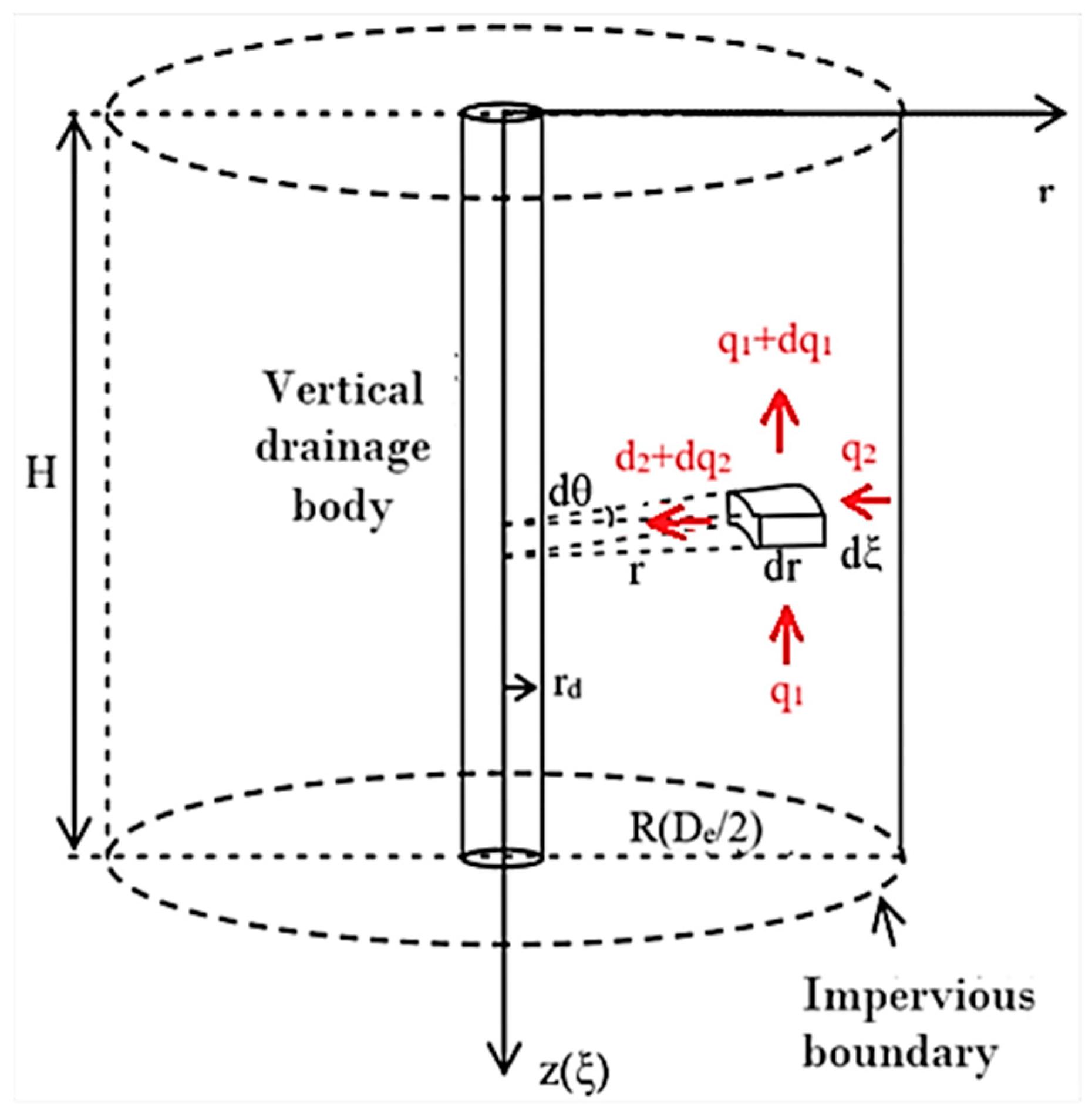
When deriving the seepage continuity equation, the relative velocity between pore water flow and soil particle movement should be considered [53,54]. By using cylindrical coordinates ( r , θ , ξ ) and analyzing a soil element during an infinitesimal time increment (as shown in Figure A1), the seepage continuity equation is derived as follows:
ε v t = e 1 + e · r ( V ξ w V s ) + 1 r r ( r · V r w )
where e represents the void ratio of the soft foundation, V s denotes the actual vertical velocity of soil particles, V ξ w signifies the actual vertical flow velocity of pore water, and V r w indicates the actual radial flow velocity of pore water.
Figure A1. Schematic diagram of seepage in the soil element of the sand drain soft foundation system.
Symmetry 17 01113 g0a1
The UH constitutive model [55] describes the stress–strain relationship of soft foundations as follows:
d ε v = d ε v e + d ε v s p
where d ε v is the volumetric strain increment, d ε v e is the elastic volumetric strain increment (see Equation (A3)), and d ε v s p is the plastic volumetric strain increment induced by stress (see Equation (A4)):
d ε v e = C s · d σ / [ ln 10 · ( 1 + e ) · σ ]
d ε v s p = C c C s ln 10 · ( 1 + e ) · M 4 M f 4 · d σ σ
where σ is the effective stress, C c is the compression index, C s is the swelling index, M is the critical state stress ratio, and M = 6 sin φ / ( 3 sin φ ) , where φ is the internal friction angle, and M f is the stress ratio at potential failure state (see Equations (A5)–(A7)):
J = σ σ c 0 · exp [ ln 10 · ( 1 + e ) · ε v s p / ( C c C s ) ]
χ = M 2 / [ 12 · ( 3 M ) ]
M f = 6 · χ J · ( 1 + χ J ) χ J
where σ c 0 is the pre-consolidation stress.
In this study, the non-Darcian seepage relationship described by a non-Newtonian exponent [56] (Equation (A8)) is simplified to Darcy’s law. The vertical and radial apparent flow velocities are expressed by Equations (A9) and (A10), respectively:
V = K · [ i i 0 ( 1 e i / i 0 ) ]
where K represents the permeability coefficient of the soft foundation and i 0 represents the non-Newtonian exponent:
V z = e 1 + e · ( V ξ w V s ) = K z · i z
V r = e 1 + e · V r w = K r · i r
where K ξ and K r are the vertical permeability coefficient and radial permeability coefficient, respectively, while i ξ and i r are the vertical hydraulic gradient and radial hydraulic gradient, respectively.
By substituting Equations (A2), (A9) and (A10) into Equation (A1), the consolidation governing equation in flow coordinates (Equation (A11)) is obtained:
1 r · r r · K r γ w · u r + ξ K ξ γ w · u ξ = λ · σ t
where u denotes pore water pressure, γ w denotes the unit weight of water, and
λ = C s + ( C c C s ) M 4 / M f 4 ln 10 · ( 1 + e ) · σ , d σ 0 C s ln 10 · ( 1 + e ) · σ , d σ < 0
By using the relationship between vertical flow coordinates (ξ) and solid-phase coordinates (z) in large-strain consolidation theory (Equation (A12)), the governing equation is transformed into solid-phase coordinates, resulting in Equation (A13):
ξ z = 1 + e
1 r · r r · ϑ r · σ r + ϕ 1 · z ϑ z · ϕ 1 · σ z + ( 1 G s ) · γ w = λ · σ t
where ϑ r = K r / γ w , ϑ z = K ξ / γ w , ϕ 1 = e ε v / ( 1 + e ) , and G s represents the specific gravity.
2. Boundary and Initial Conditions
Staged loading conditions, as described in Equation (A14) (see Figure A2 [57]), are applied:
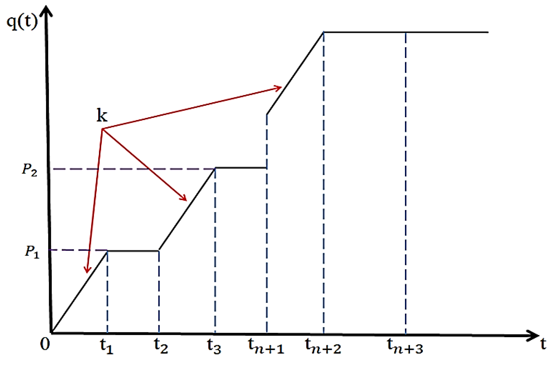
Figure A2. Schematic diagram of load–time curve under staged loading conditions.
Symmetry 17 01113 g0a2
p ( t ) = p 1 t / t c 1 , 0 t t c 1 p 1 , t c 1 t t c 2 p 1 + p 2 p 1 t c 3 t c 2 · ( t t c 2 ) , t c 2 t t c 3 p 2 , t c 3 t t c 4 p 2 + p p 2 t c t c 4 · ( t t c 4 ) , t c 4 t t c p , t t c
The mathematical framework is completed by the initial conditions (Equation (A15)) and boundary conditions (Equations (A16)–(A19)):
σ ( r , z , 0 ) = σ z 0 + ( G s 1 ) · γ w · z
where σ z 0 represents stress induced by the initial load:
σ ( r , 0 , t ) = σ z 0 + p ( t )
σ ( r d , z , t ) z = ( G s 1 ) · γ w
σ ( r d , z , t ) = σ z 0 + ( G s 1 ) · γ w · z + p ( t )
σ ( D e , z , t ) r = 0
where r d represents the diameter of the sand drain and D e represents the effective radius of the sand drain.
3. Numerical Solution Method
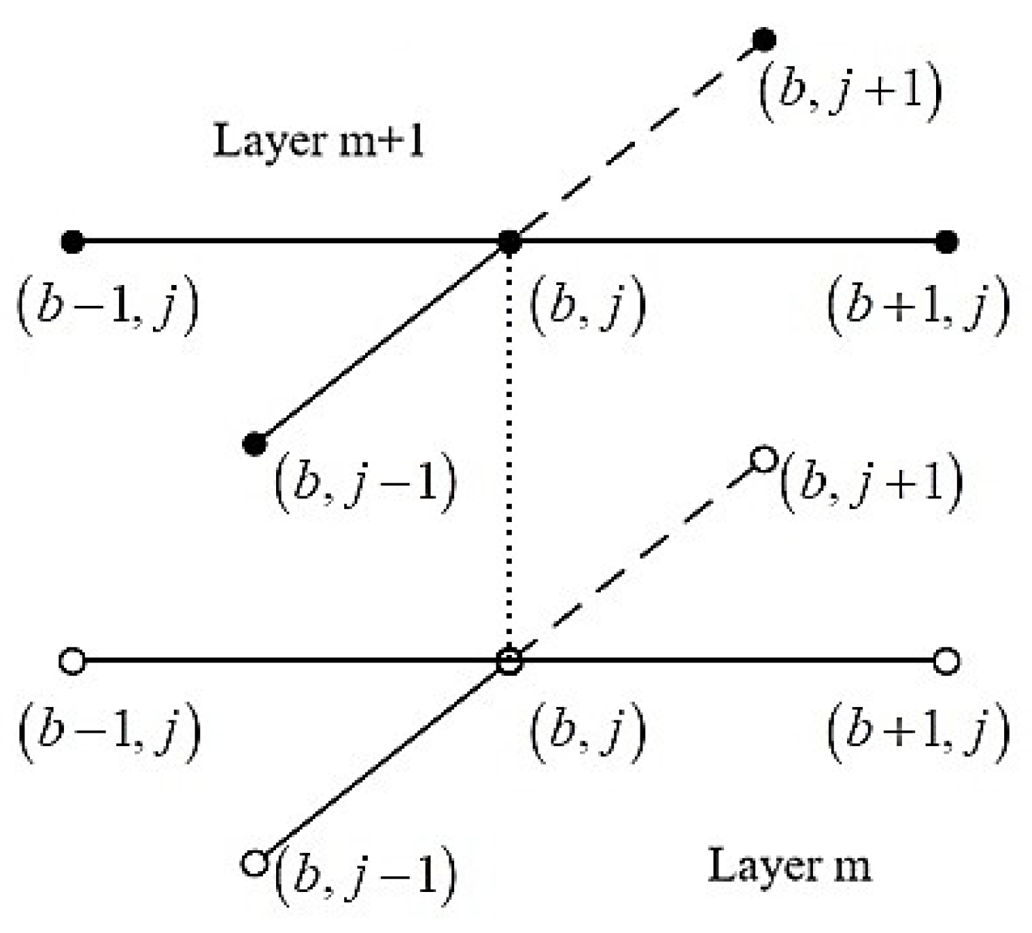
The governing equations are discretized by employing an implicit finite difference scheme [58,59]. This scheme enhances numerical stability under large-strain conditions. The initial soil thickness L is discretized into Z sublayers, and the sand drain influence zone is divided into N radial layers. For temporal discretization, times steps of size Δ t are used. As shown in Figure A3, the variable X b , j m + 1 represents its value at position ( r b , z j ) at time t = ( m + 1 ) Δ t .
Figure A3. Schematic diagram of discrete nodes.
Symmetry 17 01113 g0a3
The finite difference forms of the terms in the consolidation equation (Equation (A13)) are derived as Equations (A20)–(A22). The final discretized equation is presented as Equation (A23):
λ · σ t = λ b , j m + 1 · σ b , j m + 1 σ b , j m Δ t
1 r · r r · ϑ r · σ r = 1 r b ( Δ r ) 2 ( ϑ b + 1 / 2 , j m + 1 r b + 1 / 2 , j E b + 1 / 2 , j m + 1 ϑ b 1 / 2 , j m + 1 r b 1 / 2 , j E b 1 / 2 , j m + 1 )
ϕ 1 · z ϑ z · ϕ 1 · σ z + ( 1 G s ) · γ w = ϕ 1 b , j m + 1 Δ z [ ϑ b , j + 1 / 2 m + 1 ϕ 1 b , j + 1 / 2 m + 1 ( E b , j + 1 / 2 m + 1 / Δ z + g ) ϑ b , j 1 / 2 m + 1 ϕ 1 b , j 1 / 2 m + 1 ( E b , j 1 / 2 m + 1 / Δ z + g ) ]
σ b , j m + 1 = σ b , j m + V b , j m + 1 ( ϑ b + 1 / 2 , j m + 1 r b + 1 / 2 , j E b + 1 / 2 , j m + 1 ϑ b 1 / 2 , j m + 1 r b 1 / 2 , j E b 1 / 2 , j m + 1 )   + T b , j m + 1 ϕ 1 b , j m + 1 [ ϑ b , j + 1 / 2 m + 1 ϕ 1 b , j + 1 / 2 m + 1 ( F b , j + 1 / 2 m + 1 / Δ z + g )   ϑ b , j 1 / 2 m + 1 ϕ 1 b , j 1 / 2 m + 1 ( F b , j 1 / 2 m + 1 / Δ z + g ) ]
where, r b ± 1 / 2 = r w + ( b ± 1 / 2 ) Δ r , E b + 1 / 2 , j m + 1 = σ b + 1 , j m + 1 σ b , j m + 1 , E b 1 / 2 , j m + 1 = σ b , j m + 1 σ b 1 , j m + 1 , F b , j + 1 / 2 m + 1 = σ b , j + 1 m + 1 σ b , j m + 1 , F b , j 1 / 2 m + 1 = σ b , j m + 1 σ b , j 1 m + 1 , g = ( 1 G s ) r w , T b , j m + 1 = Δ t / ( λ b , j m + 1 Δ z ) , ϑ b ± 1 / 2 , j m + 1 = K r b ± 1 / 2 , j m + 1 / r w , ϑ b , j ± 1 / 2 m + 1 = K z b , j ± 1 / 2 m + 1 / r w , ϕ 1 b , j m + 1 = exp ε v b , j m + 1 / ( 1 + e j ) , and ϕ 1 b , j ± 1 / 2 m + 1 = exp [ ( ε v b , j m + 1 + ε v b , j ± 1 m + 1 ) / 2 ] 1 + ( e j + e j ± 1 ) / 2 .

Appendix B. Schematic Diagram of Generating Simulated Observational Data for NENSTS
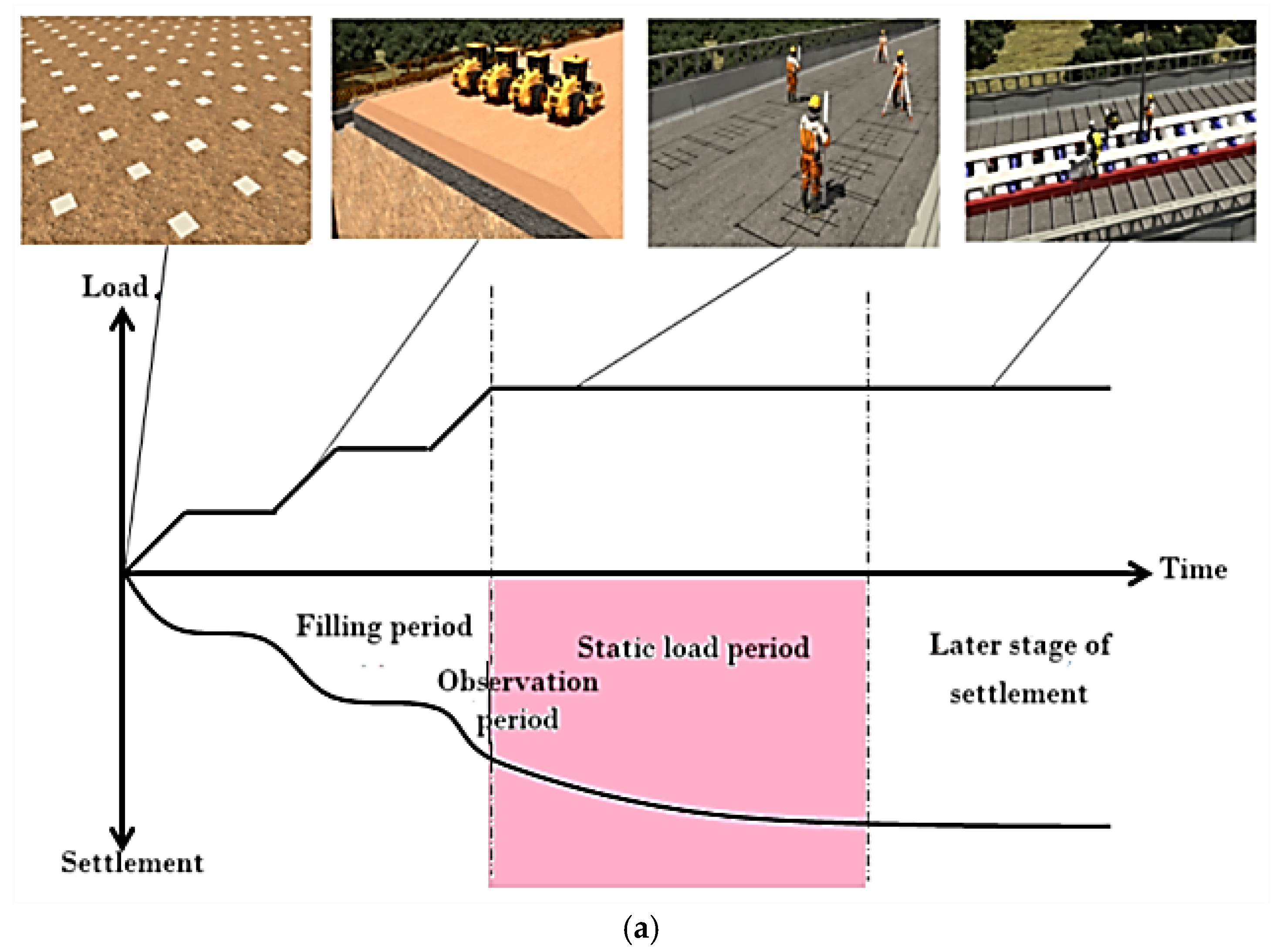
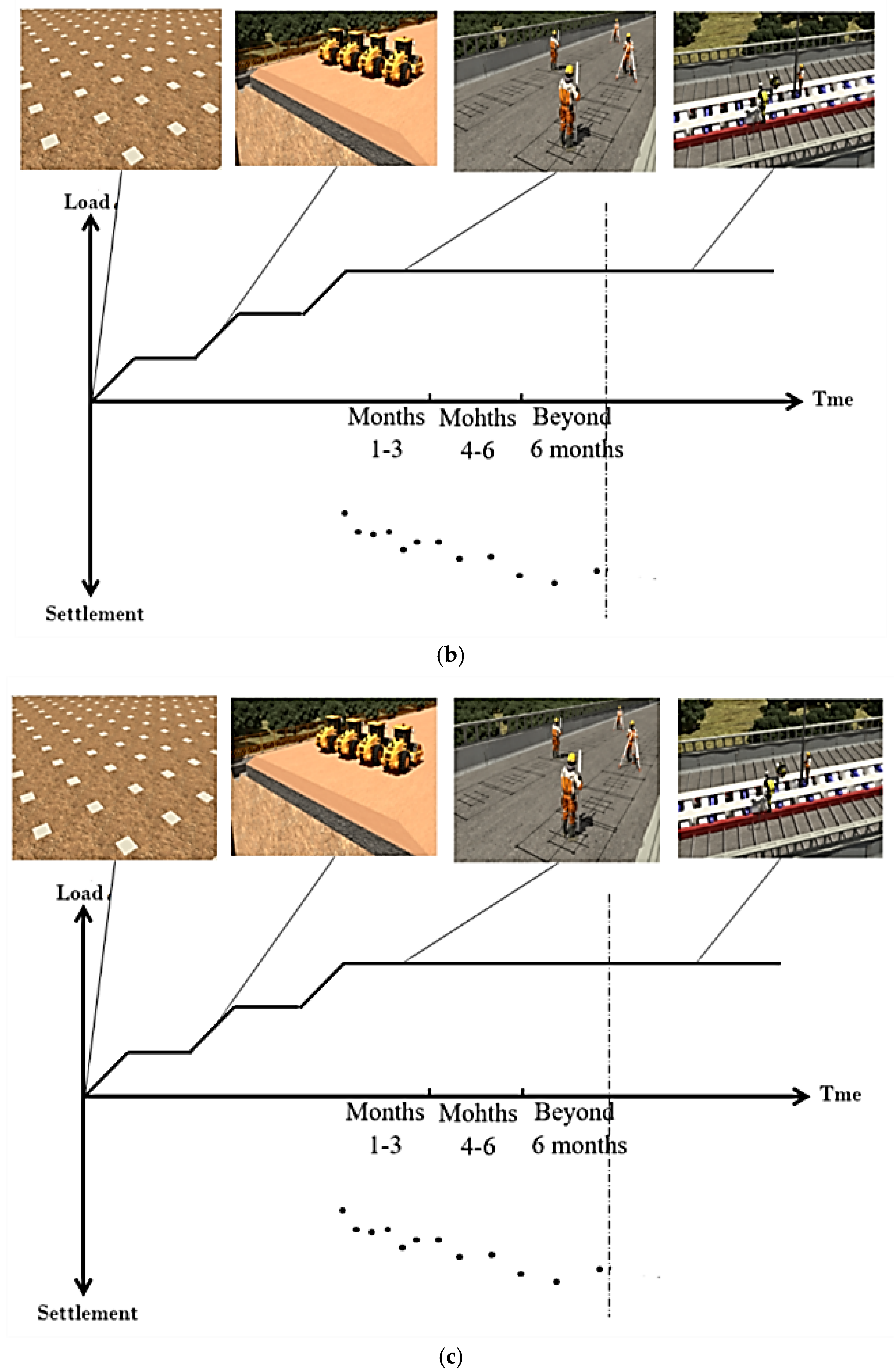
Figure A4. Schematic diagram of NENSTS simulated data generation: (a) theoretical curve truncation, (b) non-equidistant discretization, (c) random noise superposition, and (d) large-scale repeated settlement prediction.
Symmetry 17 01113 g0a4aSymmetry 17 01113 g0a4bSymmetry 17 01113 g0a4c

References

  1. Skempton, A.W.; Bjerrum, L. A Contribution to the settlement analysis of foundations on clay. Géotechnique 1957, 7, 168–178. [Google Scholar] [CrossRef]
  2. Zhai, J. Machine-learning-based road soft soil foundation treatment and settlement prediction method. Sci. Program. 2022, 2022, 3463413. [Google Scholar] [CrossRef]
  3. Indraratna, B.; Rujikiatkamjorn, C.; Ameratunga, J.; Boyle, P. Performance and prediction of vacuum combined surcharge consolidation at port of brisbane. J. Geotech. Geoenviron. Eng. 2011, 137, 1009–1018. [Google Scholar] [CrossRef]
  4. Indraratna, B.; Rujikiatkamjorn, C.; Balasubramaniam, A.S.; McIntosh, G. Soft ground improvement via vertical drains and vacuum assisted preloading. Geotext. Geomembr. 2012, 30, 16–23. [Google Scholar] [CrossRef]
  5. Ministry of Railways of the People’s Republic of China. Technical Guidelines for the Evaluation of Ballastless Track Laying Conditions for Passenger Dedicated Line Lines Tie Jianshe [2006]; No. 158; China Railway Publishing House: Beijing, China, 2006. [Google Scholar]
  6. Q/CR 9230-2016; Technical Specification for Observation and Evaluation of Settlement Deformation of Railway Engineering. China State Railway Group Co., Ltd., China Railway Publishing House: Beijing, China, 2017.
  7. Cheng, C.Q.; Sa-Ngasoongsong, A.; Beyca, O.; Le, T.; Yang, H.; Kong, Z.Y.; Bukkapatnam, S.T.S. Time series forecasting for nonlinear and non-stationary processes: A review and comparative study. IIE Trans. 2015, 47, 1053–1071. [Google Scholar] [CrossRef]
  8. Liu, Y.; Wu, H.X.; Wang, J.M.; Long, M.S. Non-stationary transformers: Exploring the stationarity in time series forecasting. In Proceedings of the Advances in Neural Information Processing Systems 35 (NeurIPS 2022), New Orleans, LA, USA, 28 November–9 December 2022; pp. 9881–9893. [Google Scholar]
  9. Juang, C.H.; Wang, L. Reliability-based robust geotechnical design of spread foundations using multi-objective genetic algorithm. Comput. Geotech. 2013, 48, 96–106. [Google Scholar] [CrossRef]
  10. Zhou, C.; Yin, K.L.; Cao, Y.; Ahmed, B. Application of time series analysis and PSO–SVM model in predicting the Bazimen landslide in the Three Gorges Reservoir, China. Eng. Geol. 2016, 204, 108–120. [Google Scholar] [CrossRef]
  11. Wang, L.Y.; Li, T.F.; Wang, P.C.; Liu, Z.; Zhang, Q. BiLSTM for predicting post-construction subsoil settlement under embankment: Advancing sustainable infrastructure. Sustainability 2023, 15, 14708. [Google Scholar] [CrossRef]
  12. Suebsombut, P.; Sekhari, A.; Sureephong, P.; Belhi, A.; Bouras, A. Field data forecasting using LSTM and Bi-LSTM approaches. Appl. Sci. 2021, 11, 11820. [Google Scholar] [CrossRef]
  13. Raubitzek, S.; Neubauer, T. A fractal interpolation approach to improve neural network predictions for difficult time series data. Expert Syst. Appl. 2021, 169, 114474. [Google Scholar] [CrossRef]
  14. Yen, N.Y.; Chang, J.W.; Liao, J.Y.; Yong, Y.M. Analysis of interpolation algorithms for the missing values in IoT time series: A case of air quality in Taiwan. J. Supercomput. 2020, 76, 6475–6500. [Google Scholar] [CrossRef]
  15. Tan, Q.L.; Wei, J.; Hu, J. Applications of wavelet neural network model to building settlement prediction: A case study. Sens. Transducers 2014, 169, 1–8. [Google Scholar]
  16. Zhang, R.J. Application of wavelet neural network in building settlement prediction. E3S Web Conf. 2020, 198, 03014. [Google Scholar] [CrossRef]
  17. Zhou, T.; Jie, Y.X.; Wei, Y.J.; Zhang, Y.Y.; Chen, H. A real-time prediction interval correction method with an unscented Kalman filter for settlement monitoring of a power station dam. Sci. Rep. 2023, 13, 4055. [Google Scholar] [CrossRef]
  18. Tao, Y.Q.; Sun, H.L.; Cai, Y.Q. Predicting soil settlement with quantified uncertainties by using ensemble Kalman filtering. Eng. Geol. 2020, 276, 105753. [Google Scholar] [CrossRef]
  19. Luo, X.L.; Gan, W.J.; Wang, L.X.; Chen, Y.; Meng, X. A prediction model of structural settlement based on EMD-SVR-WNN. Adv. Civ. Eng. 2020, 2020, 8831965. [Google Scholar] [CrossRef]
  20. Kliesch, K.; Johmann, S.; El-Mossallamy, Y.; Neidhart, T. Zur setzungsprognose bei erdbauwerken mit fester fahrbahn-erfahrungen an 43 km neubaustrecke. In Proceedings of the Entwicklungen in der Bodenmechanik, Bodendynamik und Geotechnik; Springer: Berlin/Heidelberg, Germany, 2002; pp. 333–346. [Google Scholar]
  21. Liu, J.F.; Zhao, G.T. Selection of prediction models in railway subgrade settlement assessment. Railway Eng. 2010, 11, 64–68. [Google Scholar] [CrossRef]
  22. Li, C.L. A simplified method for prediction of embankment settlement in clays. J. Rock Mech. Geotech. Eng. 2014, 6, 61–66. [Google Scholar] [CrossRef]
  23. Park, H.; Lee, S.; Hwang, D. Parameter evaluation and performance comparison of MSW settlement prediction models in various landfill types. J. Environ. Eng. 2007, 133, 64–72. [Google Scholar] [CrossRef]
  24. Sivakugan, N.; Johnson, K. Settlement predictions in granular soils: A probabilistic approach. Geotechnique 2004, 54, 499–502. [Google Scholar] [CrossRef]
  25. Chen, P.Y.; Yu, H.M. Foundation settlement prediction based on a Novel NGM Model. Math. Probl. Eng. 2014, 2014, 242809. [Google Scholar] [CrossRef]
  26. Kanayama, M.; Rohe, A.; van Paassen, L.A. Using and improving neural network models for ground settlement prediction. Geotech. Geol. Eng. 2014, 32, 687–697. [Google Scholar] [CrossRef]
  27. Sridharan, A.; Murthy, N.S.; Prakash, K. Rectangular hyperbola method of consolidation analysis. Géotechnique 1987, 37, 355–368. [Google Scholar] [CrossRef]
  28. Zeng, G.X.; Yang, X.L. Analysis of foundation subsidence of sand wells. J. Zhejiang Univ. 1959, 34–72. [Google Scholar]
  29. Asaoka, A. Observational procedure of settlement prediction. Soils Found. 1978, 18, 87–101. [Google Scholar] [CrossRef]
  30. Kong, J.; Kim, H.; Chun, B. Settlement analysis for improvement effect of soft ground method in incheon cheongna site. J. Korean GEO-Environ. Soc. 2012, 13, 19–26. [Google Scholar]
  31. Menke, W. Review of the generalized least squares method. Surv. Geophys. 2015, 36, 1–25. [Google Scholar] [CrossRef]
  32. Chai, J.C.; Shen, S.L.; Miura, N.; Bergado Dennes, T. Simple method of modeling PVD-improved subsoil. J. Geotech. Geoenviron. Eng. 2001, 127, 965–972. [Google Scholar] [CrossRef]
  33. Li, Q.F.; Wang, Z.; Yu, Y. Optimization of area replacement ratio of stone column based on robustness principle. J. Jilin Univ. Earth Sci. Ed. 2022, 52, 171–180. [Google Scholar] [CrossRef]
  34. Hu, Y.Y.; Zhou, W.H.; Cai, Y.Q. Large-strain elastic viscoplastic consolidation analysis of very soft clay layers with vertical drains under preloading. Can. Geotech. J. 2014, 51, 144–157. [Google Scholar] [CrossRef]
  35. Editorial Board of Engineering Geology Handbook. Handbook of Engineering Geology, 5th ed.; China Architecture & Building Press: Beijing, China, 2018; pp. 538–539. [Google Scholar]
  36. Leroueil, S.; Bouclin, G.; Tavenas, F.; Bergeron, L.; Rochelle, P.L. Permeability anisotropy of natural clays as a function of strain. Can. Geotech. J. 1990, 27, 568–579. [Google Scholar] [CrossRef]
  37. Adams, A.; Nordquist, T.; Germaine, J.; Flemings, P. Permeability anisotropy and resistivity anisotropy of mechanically compressed mudrocks. Can. Geotech. J. 2016, 53, 1474–1482. [Google Scholar] [CrossRef]
  38. Basak, P. Soil structure and its effects on hydraulic conductivity. Soil Sci. 1972, 114, 417–422. [Google Scholar] [CrossRef]
  39. Gao, Y.B.; Bao, W.P.; Lou, K.M. Laboratory studies on the sensitivity of layer No.4 soft clay in Shanghai. J. Tongji Univ. Nat. Sci 2015, 43, 140–145. [Google Scholar] [CrossRef]
  40. Liu, X.J.; Song, B.K.; Sun, Z.Q.; Jiao, W.X. Critical filling height of embankment over soft soil: A three-dimensional upper-bound limit analysis. Buildings 2025, 15, 395. [Google Scholar] [CrossRef]
  41. TB 10101-2018; Railroad Engineering Survey Specification. National Railway Administration of People’s Republic, China Railway Publishing House: Beijing, China, 2018.
  42. TB10001-2016; Code for the Design of Railway Subgrades. National Railway Administration of People’s Republic, China Railway Publishing House: Beijing, China, 2017.
  43. Xie, K.; Chen, X.B.; Li, T.F.; Deng, Z.-X.; Yao, J.-K.; Tang, L.-B. A framework for determining the optimal moisture content of high-speed railway-graded aggregate materials based on the lab vibration compaction method. Constr. Build. Mater. 2023, 392, 131764. [Google Scholar] [CrossRef]
  44. Zhu, Y.X.; Tian, D.Z.; Yan, F. Effectiveness of entropy weight method in decision-making. Math. Probl. Eng. 2020, 2020, 3564835. [Google Scholar] [CrossRef]
  45. Yang, Y.H. Elements of information theory. J. Am. Stat. Assoc. 2008, 103, 429. [Google Scholar] [CrossRef]
  46. Pearson, E.S. A further development of tests for normality. Biometrika 1930, 22, 239–249. [Google Scholar] [CrossRef]
  47. Pearson, E.S.I. Note on Tests for Normality. Biometrika 1931, 22, 423–424. [Google Scholar] [CrossRef]
  48. Li, G.X.; Zhang, B.Y.; Yu, Y.Z. Soil Mechanics, 3rd ed.; Tsinghua University Press: Beijing, China, 2022. [Google Scholar]
  49. Liu, Z.Y.; Cui, P.L.; Zhang, J.C.; Xia, Y. Consoidation analysis of ideal sand-drained ground with fractional-derivative merchant model and non-darcian flow described by non-newtonian index. Math. Probl. Eng. 2019, 2019, 5359076. [Google Scholar] [CrossRef]
  50. Liu, Z.Y.; Zhang, J.C.; Duan, S.Q.; Xia, Y.; Cui, P. A consolidation modelling algorithm based on the unified hardening constitutive relation and Hansbo’s flow rule. Comput. Geotech. 2020, 117, 103233. [Google Scholar] [CrossRef]
  51. Liu, Z.Y.; Xia, Y.Y.; Shi, M.S.; Zhang, J.C.; Zhu, X.M. Numerical simulation and experiment study on the characteristics of non-darcian flow and rheological consolidation of saturated clay. Water 2019, 11, 1385. [Google Scholar] [CrossRef]
  52. Nguyen, B.P.; Do, T.H.; Kim, Y.-T. Large-strain analysis of vertical drain-improved soft deposit consolidation considering smear zone, well resistance, and creep effects. Comput. Geotech. 2020, 123, 103602. [Google Scholar] [CrossRef]
  53. Zhang, M.; Wang, W.; Liu, Q.X.; Zhao, Y.M. Consolidation behaviors of double-layered vertical drains ground considering power function permeability and compressibility variation. Rock Soil Mech. 2013, 34, 3117–3126. [Google Scholar] [CrossRef]
  54. Cao, Y.P.; Sun, Z.J.; Ding, J.W.; Ji, F. Axisymmetric large-strain consolidation model for dredged clay with high water content. Chin. J. Geotech. Eng. 2016, 38, 1904–1910. [Google Scholar] [CrossRef]
  55. Yao, Y.P.; Kong, L.M.; Hu, J. An elastic-viscous-plastic model for overconsolidated clays. Sci. China Technol. Sci. 2012, 56, 441–457. [Google Scholar] [CrossRef]
  56. Swartzendruber, D. Modification of darcy’s law for the flow of water in soils. Soil Sci. 1962, 93, 22–29. [Google Scholar] [CrossRef]
  57. Cai, Y.Q.; Geng, X.Y. Consolidation analysis of a semi-infinite transversely isotropic saturated soil under general time-varying loadings. Comput. Geotech. 2009, 36, 484–492. [Google Scholar] [CrossRef]
  58. Nash, D.; Ryde, S. Modeling consolidation accelerated by vertical drains in soils subject to creep. Geotechnique 2001, 51, 257–273. [Google Scholar] [CrossRef]
  59. Liu, Z.L.; Song, P.; Li, J.S.; Li, J.; Zhang, X.-B. An optimized implicit finite-difference scheme for the two-dimensional Helmholtz equation. Geophys. J. Int 2015, 202, 1805–1826. [Google Scholar] [CrossRef]
Figure 1. Technical roadmap.
Symmetry 17 01113 g001
Figure 2. Schematic diagram of the NENSTS observation data.
Symmetry 17 01113 g002
Figure 3. Schematic diagram of the least squares principle.
Symmetry 17 01113 g003
Figure 4. Schematic diagram of statistical analysis for prediction results: (a) statistical analysis of prediction results (schematic) and (b) statistical analysis of prediction results (fine-grained).
Symmetry 17 01113 g004
Figure 5. Validation of theoretical calculation results.
Symmetry 17 01113 g005
Figure 6. Mean convergence test results of settlement prediction.
Symmetry 17 01113 g006
Figure 7. Standard deviation convergence test results of settlement prediction.
Symmetry 17 01113 g007
Figure 8. Load–time parameter values under staged loading conditions.
Symmetry 17 01113 g008
Figure 9. Scatter plots of correlation coefficients for various empirical prediction models: (a) Hyperbolic method, (b) Exponential method, (c) Asaoka method, and (d) Hoshino method.
Symmetry 17 01113 g009aSymmetry 17 01113 g009b
Figure 10. Scatter plots of systematic errors for various empirical prediction models: (a) Hyperbolic method, (b) Exponential method, (c) Asaoka method, and (d) Hoshino method.
Symmetry 17 01113 g010aSymmetry 17 01113 g010b
Figure 11. Scatter plots of random errors for various empirical prediction models: (a) Hyperbolic method, (b) Exponential method, (c) Asaoka method, and (d) Hoshino method.
Symmetry 17 01113 g011aSymmetry 17 01113 g011b
Figure 12. Scatter plot of the relationship between the CEI and EPC for various empirical models.
Symmetry 17 01113 g012
Figure 13. Distribution ranges of the CEI for various empirical models: (a) Zone ①, (b) Zone ②, and (c) Zone ③.
Symmetry 17 01113 g013aSymmetry 17 01113 g013b
Figure 14. Cross-sectional schematic diagram of soft foundation treatment at the test site.
Symmetry 17 01113 g014
Figure 15. Longitudinal sectional schematic diagram of engineering geology and soft foundation treatment.
Symmetry 17 01113 g015
Figure 16. Subgrade center settlement load–time curve.
Symmetry 17 01113 g016
Figure 17. Empirical prediction model results distribution plot.
Symmetry 17 01113 g017
Table 1. Parameter values for settlement theoretical model validation [34].
Sand drain
radius, r d (m)
Void ratio,
e
Soft soil thickness,
H (m)
Swelling index,
C s
Radial permeability coefficient,
K r (m/d)
0.0332.35960.04362.73 × 10−4
Effective radius of sand drain,
D e (m)
Water content, w (%)Soft soil density,
ρ (g/cm3)
Compression index,
C c
Vertical permeability coefficient,
K ξ (m/d)
0.525881.50.7410.94 × 10−4
Table 2. Soil parameters for the settlement theoretical model.
Soft Soil Density,
ρ (g/cm3)
Compression Index,
C c
Vertical Permeability Coefficient,
K ξ (10−4 m/d)
Effective Radius of Sand Drain,
D e (m)
Soil Soft Thickness,
H (m)
1.90.52.76/4.92/7.08/9.24/11.3/13.60.5/1.0/1.5/2.010
Void ratio,
e
Swelling index, C s Anisotropy ratio,
K r / K ξ
Vane shear strength,
C u (kPa)
Drainage type
1.670.051.1/1.3/1.5/1.7/1.930 [39]Single-sided drainage
Table 3. Deformation measurement grades and precision requirements.
Deformation Measurement GradeElevation Error (mm)
Class I±0.3
Class II±0.5
Class III±1.0
Class IV±2.0
Table 4. Subgrade settlement observation frequencies.
Observation Phase (Static Period)Frequency
Months 1–31 time/week
Months 4–61 time/2 weeks
Beyond 6 months1 time/month
Table 5. Physical–mechanical properties of soil layers.
StratumSoil Layer Thickness, h (m)Water Content,
w (%)
Soil Density,
ρ (g/cm3)
Specific Gravity,
G s
Void Ratio,
e
Plasticity Index,
I p
(%)
Coefficient of Compressibility,
a 1 ~ 2
(MPa−1)
Coefficient of Consolidation,
c v
(10−4 cm2/s)
Miscellaneous Fill (QmL)0~1.55
Soft Clay (Q4mL)0.9~2.934.71.852.740.9916.50.193.063
Sandy Soil (Q4mL)0.6~3.035.11.842.710.9910.60.366.391
Mucky Clay with Silt (Q4mL)8.8~10.147.41.732.741.3317.30.582.533
Silty Sand with Clay (Q4mL)4.6~10.527.81.912.710.816.80.158.698
Table 6. Comparison of empirical model prediction results.
Correlation CoefficientSystematic Error (%)Random Error (mm)CEI
Hyperbolic0.970. 51.750.87
Exponential0.712.740.890.64
Asaoka0.981.730.930.94
Hoshino0.980.920.530.95
Disclaimer/Publisher’s Note: The statements, opinions and data contained in all publications are solely those of the individual author(s) and contributor(s) and not of MDPI and/or the editor(s). MDPI and/or the editor(s) disclaim responsibility for any injury to people or property resulting from any ideas, methods, instructions or products referred to in the content.