Abstract
Structural magnetic resonance imaging (sMRI) is a vital tool for diagnosing neurological brain diseases. However, sMRI scans often show significant structural changes only in limited brain regions due to localised atrophy, making the identification of discriminative features a key challenge. Importantly, the human brain exhibits inherent bilateral symmetry, and deviations from this symmetry—such as asymmetric atrophy—are strong indicators of early Alzheimer’s disease (AD). Patch-based methods help capture local brain changes for early AD diagnosis, but they often struggle with fixed-size limitations, potentially missing subtle asymmetries or broader contextual cues. To address these limitations, we propose a novel augmented reality (AR)-enhanced patch-level explainable deep learning (ARE-PaLED) system. It includes an adaptive multi-scale patch extraction network (AMPEN) to adjust patch sizes based on anatomical characteristics and spatial context, as well as an informative patch selection algorithm (IPSA) to identify discriminative patches, including those reflecting asymmetry patterns associated with AD; additionally, an AR module is proposed for future immersive explainability, complementing the patch-level interpretation framework. Evaluated on 1862 subjects from the ADNI and AIBL datasets, the framework achieved an accuracy of 92.5% (AD vs. NC) and 85.9% (AD vs. MCI). The proposed ARE-PaLED demonstrates potential as an interpretable and immersive diagnostic aid for sMRI-based AD diagnosis, supporting the interpretation of model predictions for AD diagnosis.
1. Introduction
Alzheimer’s disease (AD) is an advancing neural system disorder that causes brain cells to deteriorate and perish. In the U.S., about 6.5 million of those 65 and older have AD, of which more than 70% are 75 years and older. It is also estimated that over 55 million people worldwide suffer from dementia, and 60% to 70% of the cases of dementia in the world are attributed to AD [1]. It is mental degradation characterised by a progressive deterioration in cognitive process, behaviour, and social interactions. AD typically progresses through several stages, such as the preclinical stage, mild cognitive impairment (MCI), and AD (mild, moderate, or severe), each with its symptoms and characteristics [2]. A significant decline in cognitive and physical function characterises the final stage of AD. It leads to the loss of communication, recognition, and movement control, making independent living impossible. Patients are prone to infections and complications. AD’s cause remains unknown, and no cure exists—treatment only manages symptoms and improves quality of life [3]. Early identification of AD is vital for active treatment. Diagnosis involves medical history, cognitive tests, neurological exams, and brain imaging. Brain atrophy, a key biomarker, begins before symptoms appear. Structural magnetic resonance imaging (sMRI) non-invasively detects significant brain changes linked to this process [4]. Leveraging these imaging techniques, several computer-aided diagnostic (CAD) approaches have been developed for the early detection of AD and its initial stage, MCI. The CAD approach based on sMRI involves the following key steps: choosing regions of interest (ROIs), extracting image features, and building diagnostic models for classification and analysis [5].
These sMRI-based CAD methodologies are again delineated into th evoxel-based approach, region-based approach, and patch-based approach depending on the morphological pattern in brain MRI. At the voxel level, the analysis focuses on the most minor units of the brain imaging data, enabling the highly detailed scrutiny of morphological patterns. Region-level methods, on the other hand, consider larger anatomical structures, providing a broader context for feature extraction and analysis. Patch-level approaches strike a balance between the two, examining intermediate-sized sections of the brain to identify significant morphological patterns. Each level offers unique insights, contributing to the comprehensive evaluation and diagnosis of neurological conditions.
Specifically, the voxel-level approach identifies AD-related microstructures but risks overfitting due to high feature dimensionality and limited training subjects. On the other hand, the region-level approach extracts measurable features from predefined segmented brain areas for classification, reducing dimensionality but potentially missing pathological areas and requiring expert input.
Patch-based methods utilise a median scale between voxel and region-level feature encodings to address early AD diagnosis by capturing changes in local brain regions. However, fixed-size patches either represent fine details such as edges, textures, and noise or capture larger structures, like objects or background context, but not both, leading to an incomplete representation. Further, because of deep neural networks’ inherent closed-box nature, some deep learning methods are designed to provide precise outputs for pinpointing pathological regions. In cases of brain atrophy, only specific areas in sMRI scans exhibit notable anatomical variations that strongly align with diagnostic features, while most other regions offer minimal diagnostic value. As a result, three significant challenges persist in patch-based approaches: (1) how to determine the patch size to give a complete representation of the brain atrophy, (2) how to effectively identify and select informative patches, and (3) how to integrate both local and global features with interpretability to enhance the transparency and provide immersive visualisation of the informative brain regions in AD diagnosis.
To address the abovementioned challenges, an augmented reality (AR)-enhanced patch-level explainable deep learning (ARE-PaLED) model is proposed to identify informative locations in 3D brain sMRI for AD diagnosis. As shown in Figure 1, ARE-PaLED includes three vital modules, i.e., the adaptive multi-scale patch extraction network (AMPEN), informative patch selection algorithm (IPSA), and explainable AI (XAI) with AR. AMPEN integrates voxel-based morphometry (VBM) to provide a more comprehensive view of volumetric changes and gradient magnitude analysis to detect significant alterations in the brain structure and determine appropriate patch sizes based on brain atrophy. IPSA uses an evolutionary approach, which optimises the selection of informative patches. Notably, by enabling localised patch analysis across both hemispheres, the framework can capture asymmetrical atrophy patterns, implicitly leveraging the brain’s natural bilateral symmetry—critical in identifying early signs of AD. AR-enabled XAI embraces the model’s transparency and interpretability by providing interactive and immersive visualisations.
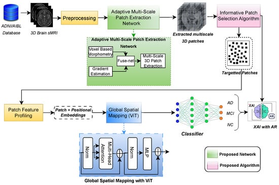
Figure 1.
Overview of proposed ARE-PaLED model, comprising the adaptive multi-scale PatchNet with FuseNet, the informative patch selection algorithm, global spatial mapping using ViT, and XAI enhanced with AR.
The proposed ARE-PaLED integrates voxel-level and patch-level approaches, combining their strengths for improved AD diagnosis. By extracting non-overlapping, multi-scale 3D patches from sMRI, ARE-PaLED identifies the most informative regions that are potentially asymmetrically affected and enhances interpretability through AR. ARE-PaLED makes three key contributions to advancing explainable deep learning in AD classification.
- The adaptive multi-scale patch extraction network (AMPEN) is proposed, which dynamically determines the optimal patch sizes to represent AD-related brain atrophy comprehensively. It automatically detects structural and volumetric changes in 3D sMRI and adjusts the patch sizes (multi-scale) based on the analysed brain regions.
- The informative patch selection algorithm (IPSA) is proposed, which uses an evolutionary approach to optimise the selection of the most informative patches. This allows for a deeper analysis of the discriminative features within each selected patch.
- The proposed method enhances patch-level explainability by incorporating AR, enabling the visualisation of discriminative patches with annotations. This improves the interpretability of classification results with immersive visualisation, aiding clinicians in their decision-making, which is crucial for AD diagnosis.
2. Literature Survey
This section summarises earlier studies on CAD for AD from sMRI data. Next, the role of vision transformer (ViT), XAI, and evolutionary algorithms related to diagnosing AD is investigated. Finally, the applications of virtual reality (VR) and AR in analysing medical images are discussed.
2.1. AD Diagnosis from sMRI
sMRI data are critical in diagnosing brain diseases, including AD. Approaches to analysing sMRI data can be broadly categorised into voxel, region, and patch-level approaches, each with unique advantages and limitations.
2.1.1. Voxel-Level Approaches
Voxel-level approaches analyse detailed, fine-grained volumetric data, providing unbiased insights into subtle anatomical changes in the brain. These methods often quantify grey and white matter densities at the voxel level, serving as input features for classification algorithms. This granularity enables the detection of minute changes, essential for understanding diseases like AD. However, voxel-based methods face challenges such as overfitting due to the higher dimensions of voxel-level features relative to the small sample sizes. Reducing dimensionality is, therefore, critical to enhancing classification precision and reliability. For example, [6] applied sparse reduced-rank regression to link gene factors with voxel-level phenotypes, significantly contributing to VBM. Foundational studies [7,8] demonstrated VBM’s ability to map grey matter atrophy in mild AD and established robust methodological frameworks for this approach. Deep learning (DL) and machine learning (ML) applications have expanded the utility of voxel-based methods. Studies [9,10,11,12,13] explored various ML and DL techniques, including tree-guided sparse coding [9], incremental learning for cortical thickness classification [10], and texture-based feature extraction for early diagnosis [13]. A notable advancement is using multi-scale deep convolutional networks for AD detection, highlighting DL’s potential in neuroimaging. Despite their promise, voxel-based methods often overlook spatial relationships between voxels, limiting their capacity to capture complex interdependencies in brain structure.
2.1.2. Region-Level Approaches
Region-level approaches focus on predefined areas of brain symmetry, such as the temporal lobes and hippocampus, which are affected by AD. These ROIs are recognised using prior knowledge, either manually or through automated atlas-based segmentation. Region-based methods benefit from reduced dimensionality and the ability to incorporate multimodal data, enhancing diagnostic accuracy. For instance, ref. [14] introduced a hypergraph-based feature selection method to classify AD using multimodal data, while [15,16] used joint regression and classification approaches for ROI analysis. Nonlinear dimensionality reduction techniques [17] and unsupervised learning frameworks [18] have further improved classification performance. Recent innovations include attention-guided hybrid networks [19] that direct the model’s focus to informative ROIs and methods emphasising continuous evolution in diagnostic processes [20,21,22]. However, region-based approaches often miss localised atrophy and intricate inter-regional relationships, limiting their ability to detect subtle abnormalities critical for early AD diagnosis.
2.1.3. Patch-Level Approaches
Patch-based methods offer a middle ground, analysing localised brain segments across the brain’s symmetry to detect atrophy and precisely classify dementia. These approaches divide MRI scans into patches, allowing focused analysis of smaller brain areas. Significant advancements have been made in this domain. Ref. [23] proposed a hierarchical fully convolutional network (H-FCN) that simultaneously detects atrophy to diagnose AD, while [24] applied multiple instance learning for robust dementia classification. Patch-based methods have also been used for anatomical landmark detection [25] and ensemble classification [26,27]. Deep learning frameworks have further enhanced the interpretability and accuracy of patch-based approaches. For instance, interpretable models [28,29] and supervised switching auto encoders [30] have been employed for single-slice and regional analyses. Methods leveraging attention mechanisms [31] and genetic algorithms [32,33,34] illustrate the versatility of patch-based frameworks in handling complex neuroimaging data. Despite their advantages, patch-based methods face challenges such as arbitrary patch placement, which may introduce noise or overlook critical regions. Maintaining spatial connections between patches and highlighting discriminative characteristics without losing global context remains challenging.
2.2. Evolutionary Approach
Evolutionary approaches in diagnosing AD leverage deep learning and genetic algorithms (GAs) to enhance classification accuracy and interpretability. Ref. [35] utilises GA in feature selection of multimodal data for AD diagnosis along with SVM. Similarly, GA-MADRID [36] and multimodal neuroimaging with an evolutionary RVFL classifier [37] highlight evolutionary methods’ power in combining imaging modalities to improve precision. Study [38] demonstrates the application of GAs for feature selection in FDG-PET imaging and logistic regression, showcasing their adaptability to complex neuroimaging data. However, the effectiveness of evolutionary algorithms depends on designing fitness functions that balance accuracy, interpretability, and computational efficiency, posing significant challenges.
2.3. ViTs
The use of ViTs in AD research has expanded significantly, showcasing their versatility in diagnostic tasks. A lightweight ViT framework [39] enables efficient 3D hippocampus segmentation with multiscale convolution attention, enhancing spatial feature representation. ViTs combined with convolutional architectures and channel attention [40] classify AD using spectrograms, while a gradient centralisation optimiser [41] improves performance on small datasets. A unified multimodal transformer framework [42] integrates diverse data for comprehensive assessment. Ref. [43] uses an attention mechanism along with ViT for efficient feature learning and classification of dementia while combining ViTs with Bi-LSTM models [44] leverages temporal and spatial dependencies, illustrating innovative approaches for precise AD diagnosis from MRI data.
2.4. XAI
Recent advances in XAI for AD focus on enhancing interpretability and clinical utility. A novel neural network [45] improves diagnosis accuracy through interpretable features, addressing traditional models’ black-box nature. A 3D residual self-attention network [46] localises atrophy and diagnoses AD using MRI. Patch-based frameworks [47], such as sMRI-PatchNet [29], offer visualised decision-making paths for clinicians. Graph convolutional networks [48] explain predictions, aiding clinical decisions. Multimodal XAI frameworks [49,50] integrate diverse data sources, providing comprehensive insights for AD prediction and management, underscoring the importance of interpretable models in advancing diagnostic precision.
2.5. Medical AR and VR
VR and AR are transforming medical image processing by enhancing visualisation and diagnostic accuracy. VR facilitates immersive environments for AD diagnosis in the metaverse [51]. At the same time, ref. [52] explores the integration of virtual reality (VR) in diagnosing and treating neurological disorders, emphasising its role in enhancing patient engagement and therapy outcomes. The review [53] found that VR-based interventions showed promising results in enhancing executive functions and visuospatial skills, particularly in both acute and neurodegenerative conditions. Applications in biomedical imaging [54] highlight their potential to revolutionise diagnostics with dynamic visualisations. AR innovations [55] enhance learning and decision-making, and platforms like COVI3D [56] integrate real-time automated classification and visualisation, demonstrating substantial advancements in medical image analysis and interpretation.
The reviewed literature highlights significant advancements in patch-level analysis, XAI, and AR for AD diagnosis using 3D sMRI; however, these technologies have largely evolved in isolation. Patch-based methods offer localised insights but struggle with arbitrary patch placement and lack spatial coherence, while XAI improves model transparency yet remains limited in immersiveness and spatial depth. Although AR has shown potential in medical visualisation, its application for interpreting deep learning-based neuroimaging models is underexplored. Addressing this gap, the proposed system is designed to support AD diagnosis from 3D sMRI by providing interactive and spatially aligned visuals that help bridge the gap between model predictions and clinical interpretation.
3. Subjects and Image Pre-Processing
This section explains the dataset used in this study, including its characteristics and subject distribution, followed by a detailed description of the image preprocessing methods applied to the sMRI data for the study.
3.1. Dataset
This work studied two publicly available datasets, including 1173 year one sMRI scans from ADNI-2 and ADNI-3 and 689 baseline sMRI scans from AIBL. Table 1 summarises the subjects’ background information for the datasets considered above.

Table 1.
Demographic and clinical characteristics of participants across datasets.
ADNI 2 datasets taken for the study include the year 1 T1-weighted 3T sMRI scans of 652 subjects. The subjects are categorised into three groups: normal controls (NC), MCI, and AD. Clinical tools like the Mini-Mental State Examination (MMSE) and clinical dementia ratings (CDR) are also used. To conclude, the year 1 ADNI-2 dataset consists of 209 individuals categorized as NC, 248 individuals identified as having MCI, and 195 subjects diagnosed with AD.
The ADNI 3 datasets taken for the study include the year 1 T1-weighted high-resolution 3T sMRI data from 521 participants. These subjects were carefully curated to meet clinical standards similar to ADNI-2 and are categorised into three groups: 165 NC subjects, 197 individuals with MCI, and 159 individuals with AD.
The baseline AIBL dataset considered for validation includes T1-weighted 1.5T or 3T sMRI scans from 689 participants, of whom 93 have been diagnosed with AD, and the remaining 596 are classified as NC. Demographic information, comprising MMSE scores, age, gender, and CDR, is accessible for all the AIBL subjects in the study.
MCI Subgroup Labelling
For some MCI patients, classification was further carried out based on their progression into AD within the first 24 months following the first year’s assessment. Individuals who have continuously been classified as MCI over all time points (ranging from 0 to 96 months) were called stable MCI (sMCI), while those who developed AD in less than three years were referred to as progressive MCI (pMCI). Here, there is a possibility of classification bias because some individuals are classified as having sMCI solely because they have not yet converted, not because they will never convert; additionally, many MCI patients have follow-up data of less than three years, and it is unclear if they will eventually develop AD, which raises questions about their actual diagnostic status. Hence, there is the need for a strategy to label the MCI subgroup. Although our model treats MCI as a single class for classification against AD and NC, and does not distinguish between pMCI and sMCI, strict criteria have been established to ensure the integrity of the MCI labels. The following standards are imposed when building the MCI subset of our dataset to ensure its integrity.
- Subjects who had only been converted to AD within three years of baseline were given pMCI. Subjects who had maintained as MCI for at least three years straight without conversion were given sMCI.
- Subjects whose actual progression status could not be ascertained, those with fewer than three years of follow-up, and those with no apparent conversion were excluded from both pMCI and sMCI.
- By eliminating such ambiguous subjects, the possibility of incorrectly classifying unobserved pMCI as sMCI is avoided.
This strategy made sure that the MCI class used in our tests included cases that were consistently categorised.
3.2. Image Preprocessing
Pre-processing was performed on the original sMRI, to improve feature learning and classification; data were retrieved from ADNI. First, 3D grad warp correction was used to correct the geometry for gradient nonlinearity. Next, B1 non-uniformity correction was applied to correct for intensity non-uniformity. After that, non-brain tissues were removed using skull stripping, which separated the brain tissue for additional examination. The pictures were oriented along the anterior commissure (AC)–posterior commissure (PC) axis to standardise brain orientation. Each sMRI was subjected to an affine registration, which aligned it to the Colin27 template and removed global linear variations like translation, scaling, and rotation. Lastly, the MRIs were down-sampled to 160 × 192 × 160 to balance computational efficiency and detail.
4. Methodology
This section explains the proposed ARE-PaLED framework, detailing its architecture, the process of discriminant patch extraction using an evolutionary approach, and the integration of explainability through AR projection with proposed algorithms.
4.1. Overall Method
An AR-enabled patch-level explainable deep learning framework, ARE-PaLED, is proposed (as shown in Figure 1) with an evolutionary approach to identify the discriminant patches extracted from the sMRI of the entire brain volume for AD detection. It initially employs the AMPEN, which has two fully convolutional networks (FCNs) and one convolutional neural network (CNN) to generate a consolidated feature map encompassing the entire 3D brain MRI. The first FCN is responsible for producing voxel-wise p-value maps using VBM. Subsequently, the second FCN extracts features utilising estimation techniques. Finally, the CNN integrates the statistical significance information derived from VBM (p-values) with the gradient features, resulting in a more comprehensive and informative feature map. Based on the values in the feature map (collectively referred to as z-scores), non-overlapping patches of varying sizes are extracted from the 3D brain sMRI. The most discriminative patches are then selected using the proposed IPSA, which applies an evolutionary approach to determine the fitness value of each extracted patch. Patches with the highest fitness values are chosen as discriminant patches for further analysis. These selected patches undergo local feature analysis and global spatial mapping, after which they are provided with a classifier to distinguish AD, MCI, and NC patients. Additionally, interpretability at the patch level is enhanced by projecting the informative patches in AR. While the architecture integrates standard PyTorch 2.3.0 modules for general operations such as convolution and transformer encoding, the AMPEN (given in Algorithm 1) and IPSA (given in Algorithm 2) are specifically designed and proposed in this study. These are also highlighted in the green blocks and pink blocks, respectively, of Figure 1.
| Algorithm 1 Proposed Adaptive Multiscale Patch Extraction Algorithm |
|
| Algorithm 2 Proposed Informative Patch Selection Algorithm |
|
4.2. Adaptive Multi-Scale Patch Extraction
4.2.1. Voxel-Based Morphometry (VBM)
The FCN designed for VBM on 3D brain MRI scans consists of six convolutional layers. The input to the network is a 3D brain MRI scan with a shape of (D, H, W, 1), where D, H, and W characterise the scan’s depth, height, and width, and 1 represents the single-channel grayscale intensity values. The network begins with four 3D convolutional layers, each kernel of size 3 × 3 × 3, with padding applied to preserve the input dimensions. Every convolutional layer is accompanied by batch normalisation and a rectified linear unit (ReLU) activation function to introduce non-linearity.
After the convolutional layers, max-pooling is applied using a filter size of 2 × 2 × 2 in between specific layers to reduce the spatial dimensions, allowing the network to learn more abstract feature representations. This is followed by two additional 3D convolutional layers with up-sampling to restore the original 3D spatial structure of the input scan, ensuring voxel-wise outputs that align with the input.
Finally, the network concludes with a 1 × 1 × 1 convolutional layer, which produces the voxel-wise output corresponding to p-values. The function applied to the final layer is a sigmoid activation to guarantee that the output values are within the range of 0 to 1.
4.2.2. Gradient Estimation (GE)
The FCN designed for GE on 3D brain MRI scans is structured to estimate voxel-wise gradient magnitudes, which can be used to identify discriminative locations in the various region of brain symmetry. The network starts with two 3D convolutional layers, each kernel of size 3 × 3 × 3 to capture low-level features, succeeded by batch normalisation and ReLU activation for non-linearity. After each convolution, a layer of size 2 × 2 × 2 max-pooling is applied to down-sample the spatial resolution, allowing the network to focus on more abstract and complex features.
Following the down-sampling layers, two more 3D convolutional layers refine the learned features further, and up-sampling layers restore the spatial resolution to match the input. These up-sampling layers ensure that the input image corresponds to the final output voxel-wise. The concluding layer of the network uses a 1 × 1 × 1 convolutional layer with three filters to estimate the gradient in the three directions (x, y, and z). The outcome is a three-channel map, where each channel corresponds to the gradient in one of these directions.
The network uses the Euclidean norm to compute the gradient magnitude for each voxel. of the gradient vectors. This can be computed as part of the network or as a post-processing step. The network output is a single-channel 3D volume in which each voxel contains the gradient magnitude, representing the sharpness of structural changes at that location.
The designed FCN is trained with a mean squared error loss function, and efficient weight updates are performed using the Adam optimiser. This structure allows the network to estimate the gradient magnitudes across the 3D MRI scan, with its convolutional, pooling, and up-sampling layers.
4.2.3. Fuse-Net of VBM and GE
Inspired by the need to fuse both statistical and structural information from brain MRI scans, a Fuse-Net structure is designed to fuse the outputs of two fully convolutional networks (FCNs), one for VBM and the other for GE, to produce normalised z-scores, which highlight discriminant regions in 3D brain MRI. The network begins by taking two inputs, the voxel-wise p-value map from the VBM FCN and the gradient magnitude map from the GE FCN; both are single-channel 3D volumes with the shape (D, H, W, 1). These inputs are concatenated along the channel axis, forming a two-channel input , which contains both statistical significance and structural information.
After concatenation, a series of 3D convolutional layers is applied to learn the joint features between the two modalities. Each convolutional layer uses a kernel size of 3 × 3 × 3 and applies the ReLU activation function. Batch normalisation follows each convolution to stabilise training, and pooling layers with 2 × 2 × 2 max-pooling filters are intermittently applied to down-sample the feature maps, allowing the network to capture abstract and larger-scale patterns.
Up-sampling layers restore the spatial dimensions to match the input and maintain the original spatial resolution. The up-sampling is applied after the down-sampling layers to ensure that the final output corresponds voxel-wise to the original 3D MRI scan. These up-sampled features are passed through a final 3D convolutional layer with a filter of size 1 × 1 × 1, reducing the feature map to a single-channel output.
The output of this final convolutional layer is a 3D volume containing raw voxel-wise values, which are then normalised into z-scores. This z-score normalisation ensures that the network output is standardised, providing a voxel-wise representation of how much each region deviates from the mean, thus identifying discriminant areas in the brain. The final output is a 3D map of normalised z-scores , which highlights the brain areas with significant structural or statistical deviations.
Combining the p-value maps and gradient magnitudes, this CNN provides a robust method for identifying discriminant locations in 3D brain MRI, offering a joint statistical and structural analysis. The network efficiently processes both inputs to extract meaningful patterns and provide a normalized voxel-wise measure of discriminant significance, which is crucial for analysing brain abnormalities.
4.2.4. Dynamic 3D Patch Extraction
The CNN structure is designed to extract non-overlapping 3D patches from a brain MRI based on normalised z-scores. It dynamically adjusts the patch size according to the significance of the z-score. A normalised z-score map, representing voxel-wise z-scores for the entire 3D brain MRI, is provided as input to the designed CNN. For voxels where the z-score is greater than 1, the network extracts a larger patch of size 32 × 32 × 32, as these regions indicate higher discriminative significance. In contrast, for voxels where the z-score is less than or equal to 1, a minor patch of size 16 × 16 × 16 is extracted, as these regions are considered less discriminative.
A custom layer is implemented within the CNN to achieve this dynamic patch extraction. This layer scans the z-score map and determines the appropriate patch size for each voxel. If Z(V) > 1, a 32 × 32 × 32 patch centered at voxel V is extracted, and if Z(V) < 1, a 16 × 16 × 16 patch is extracted. The patch extraction process is non-overlapping, meaning no two patches share the same voxels. This is ensured by setting the extraction stride equal to the patch size (32 or 16), ensuring that patches are spaced apart based on their respective sizes.
The network begins by using a convolutional layer to detect regions where z-scores are higher than 1, acting as a filter to highlight more discriminative regions. Based on this filter, the custom extraction layer selects the patch size accordingly. Larger patches are extracted from areas of greater significance, while smaller patches are extracted from regions of lesser interest. After extraction, the patches can be passed through additional convolutional layers to extract higher-level features for tasks such as segmentation or classification.
This adaptive method is shown in Algorithm 1. It allows efficient 3D brain MRI data processing, focusing computational resources on regions with higher z-scores (potentially indicating abnormalities) while minimising attention to less significant regions. Importantly, by extracting patches from both hemispheres, the method enables implicit comparison across anatomically corresponding areas, allowing downstream tasks to detect asymmetrical structural changes. The network’s final output is a set of non-overlapping 3D patches, varying in size based on the z-score, which can then be used for further analysis in medical image processing including the identification of symmetry-related atrophy patterns.
Thus, the proposed AMPEN performs dynamic, non-overlapping, multi-scale patch extraction by jointly leveraging voxel-wise statistical significance (derived from voxel-based morphometry) and gradient-based feature sensitivity. Unlike traditional methods that rely on fixed patch sizes or uniform sampling, AMPEN adaptively determines both patch size and location based on the degree of region-specific brain atrophy, allowing the model to concentrate on structurally and functionally salient brain areas.
Importantly, AMPEN integrates voxel-level and patch-level information, enabling the system to retain fine-grained spatial detail while also capturing broader regional context. This dual-resolution strategy enhances both classification performance and model interpretability by grounding predictions in anatomically meaningful features.
This integrated, adaptive approach to multi-scale patch extraction, guided by both statistical and gradient based cues, represents a key innovation and a novel contribution to explainable deep learning in neuroimaging-based AD diagnosis.
4.3. Informative Patch Selection
The IPSA (given in Algorithm 2) aims to identify the most informative 3D patches from brain MRI data using a combination of z-scores, SHapley Additive exPlanations (SHAP) coefficients, and an evolutionary approach. This methodology lets denote a subsample of patches selected for network training while X represents the aggregated vector of features from all possible patches. The fitness of each subgroup, F(), measures its usefulness for classification tasks. This fitness score is formulated as a weighted sum of various components, as shown in Equation (1).
Here, the term quantifies the statistical significance of the patches. This ensures that patches selected from regions with higher z-scores are prioritised, as they likely correspond to more clinically relevant areas. The second component, , utilises SHAP values to gauge an individual patch’s influence on the model’s classification. SHAP values provide insight into how much each patch influences the overall classification decision, making them vital for interpretability. The final term, , penalises redundancy among selected patches, discouraging overlap and promoting diversity. This is particularly important in imaging contexts, where multiple patches may capture similar anatomical features.
Algorithm 2 operates as follows: It begins by creating an initial population of chromosomes, each demonstrating a subset of patches. In each generation, the algorithm calculates the fitness of every individual chromosome using the formulation in Equation (1). The best-performing chromosomes are then selected as parents for the next generation.
Crossover operations are performed on these parent chromosomes to create offspring, combining features of selected patches from both parents. The mutation is also applied to introduce variability, allowing for the exploration of new combinations of patches. The new generation of chromosomes is formed by selecting the best individuals from both the parents and offspring, a strategy known as elitism.
This iterative process continues for several generations to maximise the fitness function. The result is the best chromosome Copt, which identifies the optimal subset of informative patches that balance statistical significance and interpretability while minimising redundancy.
4.4. Patch Feature Profiling
The CNN designed for local patch feature analysis of non-overlapping 3D multi-scale patches from 3D brain sMRI scans begins by accepting two different patch sizes: 16 × 16 × 16 and 32 × 32 × 32. Each patch is independently processed, with the input shape being 16 × 16 × 16 or 32 × 32 × 32, representing grayscale intensity values. The CNN consists of three 3D convolutional layers with 3 × 3 × 3 filter size, followed by ReLU activations to capture local spatial features. Padding is applied to preserve the input dimensions during convolutions. As the network progresses, filters increase (e.g., from 32 to 64 and 128), allowing the network to capture more abstract and complex features.
To reduce spatial dimensions and extract essential features, 3D max-pooling layers are applied with a kernel size 2 × 2 × 2, halving the spatial resolution while retaining critical information. After the final convolutional and pooling stages, a global pooling layer (global max pooling) converts the 3D feature volumes from each patch into single-dimensional feature vectors. These feature vectors summarise the local information from each patch. This vector represents the local features extracted by the CNN and is ready for further analysis.
This architecture is optimised to extract informative features from both fine-grained (16 × 16 × 16) and coarse-scale (32 × 32 × 32) patches, providing a compact representation of local brain structures within the 3D sMRI data.
4.5. Global Spatial Mapping
The global spatial mapping is performed using ViT. It processes the CNN-derived patch embeddings, which already include positional information. Instead of explicitly adding positional encodings in the transformer, the tokens fed into the ViT include patch and positional representations from the CNN output.
The input token to the transformer, corresponding to the ith patch, is defined as . is the CNN-extracted embedding, which already encodes positional and feature information through learned convolutional features. The entire input sequence to the ViT consists of all positional-encoded tokens , one for each patch.
The ViT comprises multiple transformer encoder layers to model the global relationships between patches. The core of each encoder layer is the multi-head self-attention mechanism, which computes how each patch is related to every other patch. For a given token, self-attention is computed using the formulation in Equation (2).
Q is the queries, K is the keys, and V is the values resulting from the input tokens through learned projection matrices. The dimension of the keys is , and the softmax operation normalises the attention scores. In multi-head attention, multiple sets of attention heads are computed in parallel. After self-attention, a feed-forward network (FFN) is fed with the output that applies a non-linear transformation as shown in Equation (3).
where and are weight matrices and and are biases. This FFN is applied independently to each token. Additionally, residual connections and layer normalisation are used by each transformer encoder layer to improve the learning process and stabilise training. The ViT’s output, after multiple transformers layers, provides a globally refined representation of the 3D brain sMRI. This globally aware output from the ViT represents local details and long-range spatial interactions across the brain.
4.6. Classifier
The fully connected layer designed for multi-class classification (distinguishing among AD, MCI, and NC) receives its input from the ViT, which has processed the global spatial features of the brain sMRI. The ViT output, the refined sequence of patch tokens, is first flattened into a vector of features. The fully connected layer completes the classification by receiving this vector as input. It also consists of one or more dense layers.
The first step is to project the ViT’s output to a lower-dimensional space using a dense layer, as shown in Equation (4).
where z is the input feature vector from the ViT, is a learned weighted matrix, is the term for bias, and the activation function is ReLU that introduces non-linearity. This transformation reduces the dimensionality of the input while capturing the most discriminative features.
The result produced in this layer is carried to another dense layer, typically without an activation function, to project the features onto the target class labels (three in this case, AD, MCI, and NC). The final output logits are given by Equation (5).
and are the weight matrix and bias for the output layer, and O contains each class’s raw prediction scores. A softmax activation function is applied to convert these logits into probabilities for each class. This function ensures that the sum of the probabilities across all three classes is 1, making it suitable for multi-class classification.
The final predicted class is assigned based on the maximum predicted probability. Through its series of transformations, this fully connected layer ultimately distinguishes among AD, MCI, and NC using the global spatial features extracted by the ViT.
4.7. Patch-Level Explainability with AR
In proposed ARE-PaLED network, the selected informative patches are projected using AR to provide an interactive and semi-immersive visualisation of critical brain regions associated with AD. AR integration is achieved through the Unity platform combined with the AR Foundation.
The AR system for XAI receives patch-level information from two core components of the pipeline. First, the voxel-wise z-scores from IPSA that identify anatomically significant patches that exhibit high statistical deviation across the brain volume. Second, a classification label is assigned by the classifier based on the selected patches and learned spatial patterns.
To enable intuitive, marker-based AR explainability, the WebAR pipeline for the proposed system is extended using frameworks such as AR.js, A-Frame, or MindAR. Upon detecting a printed fiducial marker, the system queries a backend API to retrieve patch metadata, including MNI-normalised 3D coordinates, z-scores, and predicted class labels. Each patch is then projected into 2D screen space using Three.js’s camera projection matrix and visualised as a lightweight rectangular outline anchored to the physical marker. Box centers are computed via a linear transformation from MNI coordinates to marker space. To ensure high frame rates on web and mobile devices, each overlay is rendered without lighting or shadows. An A-Frame raycaster module listens for user interactions. When a user taps on a patch, a dashed bounding box is overlaid, and a contextual label slides into view, displaying the patch’s z-score and class confidence. Patch elements are loaded efficiently in small batches using request IdleCallback to avoid blocking the main rendering thread.
The AR system for XAI supports:
- 2D interactive viewing: Users move their device over a marker to inspect the patch layout projected onto the brain model within a controlled 2D view.
- Patch highlighting: Patches identified by IPSA that contribute to the class prediction are highlighted.
- Metadata popups: Tapping a patch reveals its IPSA-derived z-score and ViT-predicted class label, offering transparency into both statistical significance and model reasoning.
By combining statistical evidence with deep model predictions and projecting them through an AR module, the proposed system offers intuitive, spatially grounded insights that support clinical decision-making by linking model outputs to visually interpretable brain regions.
4.8. Hyperparameter Tuning and Validation
Statistical significance (z-scores), SHAP interpretability, and patch redundancy are balanced by treating β, δ, and γ in the fitness function (Equation (1)) as hyperparameters. A grid search is performed over the ADNI training set using nested 5-fold cross-validation, where β and δ are swept with weights of 0.1, 0.5, 1.0, and 2.0, and γ over weights of 0.01, 0.1, 0.5, and 1.0. The triplet is selected with the maximised mean AUC on the inner validation folds. The result is β = 1.0, δ = 1.0, and γ = 0.1. To guarantee that weight selection was based on discriminative performance optimisation, these values were fixed in all ensuing trials, including cross-dataset evaluations.
4.9. Loss Function
To enhance the model’s focus on meaningful, discriminative patches, informative patches are selected based on z-scores and SHAP coefficients, indicating feature importance. To achieve this, weight regularisation (weight decay) can be integrated into the loss function, penalising large weights and promoting a simpler model.
The softmax loss is the most appropriate loss function for this multi-class classification task. This function computes the loss by computing the divergence of the predicted probability distribution from the actual class labels. Additionally, class weighting can be applied if there is a class imbalance, ensuring that the model places appropriate emphasis on underrepresented classes. Thus, the cumulative loss function for the network is shown in Equation (6).
represents class weights, denotes accurate labels, indicates predicted probabilities, and λ is the regularization term.
4.10. Implementation
The proposed ARE-PaLED is developed in Python 3.8 using the PyTorch 2.3.0 library, ensuring a robust and efficient model training and evaluation environment. To prevent overfitting, batch normalisation is applied after each convolutional layer, enhancing model stability and convergence. The AMPEN extracts image patches from distinct brain regions, capturing various anatomical variations and increasing the training data’s diversity. The training process uses cross-validation using five split partitions on 80% of the dataset, reserving 20% for testing and ensuring a rigorous assessment of model performance. The model’s trainable parameters, like batch size, learning rate, and patch count (e.g., 50 patches), are optimised during validation for best results.
The model is trained over 100 epochs using the Adam optimiser with a learning rate 0.001, achieving a balance between computational efficiency and learning performance. The system configuration for model execution includes an NVIDIA QUADRO P5000 GPU, 64 GB RAM and a CPU of Intel(R) Xeon(R) W-2133 at 3.60 GHz, providing the computational power needed for deep learning tasks. Unity3D 6.0 and the AR Foundation package are utilised for interpretability to project the discriminative patches in AR.
5. Results and Analyses
This subsection presents the experimental analysis conducted to evaluate the effectiveness of the proposed ARE-PaLED framework. It includes a detailed explanation of the performance metrics used to assess classification accuracy and model robustness. Furthermore, the framework is compared against several state-of-the-art approaches to highlight its relative advantages. A comprehensive comparative analysis is conducted based on the quantitative results. Additionally, cross-dataset validation is performed to demonstrate the generalisability and adaptability of the proposed method across different neuroimaging datasets.
5.1. Experimental Setup
The proposed ARE-PaLED model was validated on several AD-related diagnostics tasks, including AD classification (AD vs. NC) and MCI classifications (MCI vs. NC and MCI vs. AD). Four metrics are considered to assess the performance of the classification: accuracy (ACC), sensitivity (SEN), specificity (SPE), and area under the receiver operating characteristic curve (AUC). The metrics used are shown in Equations (7)–(9).
Here, TP is true positive, TN is true negative, FP is false positive, and FN is false negative. The area under the curve (AUC) is calculated for each pair (TPR = SEN, FPR = 1 − SPE) by changing the classification thresholds across prediction scores from the proposed ARE-PaLED trained network.
5.2. Comparison Approaches
The proposed ARE-PaLED was experimentally evaluated against three traditional machine learning-based approaches. The first approach uses region-based features, specifically, regions of interest (ROI). The second approach employs voxel-based features, referred to as VBM. The third approach utilises patch-based features. Additionally, it is contrasted with DA-MIDL, the most effective deep learning-based approach.
5.2.1. ROI
In this study [15], prior research on processing registered MR images using the HAMMER algorithm was followed [57] for deformable registration, segmenting them into multiple regions based on a template containing 93 manually labelled regions of interest (ROIs). With the aid of FAST algorithm in FSL package, each sMRI was divided into grey matter (GM), white matter, and cerebrospinal fluid. GM volume in each region is quantified, and then these GM volumes are normalised by the total intracranial volume. AD-related classification was performed using a trained linear support vector machine (SVM) classifier using feature vectors from these normalised ROI features.
5.2.2. VBM
This VBM approach [8] involves processing high-dimensional voxel-wise features, necessitating dimensionality reduction. Each sMRI undergoes spatial normalisation to a standard stereotactic brain space, specifically, the template of Colin27, to measure local GM density as a voxel feature. A t-test compares differences of AD patients from NC for every voxel, facilitating feature selection. Linear SVM classifiers were constructed to diagnose AD from the selected voxel features.
5.2.3. Patch-Based Method
As in [25], the patch-based method was used, where a feature extraction approach was landmark-based and employed for diagnosing AD from sMRI data. Group comparisons of local morphological features were conducted to identify brain areas with substantial group differences in AD patients from healthy controls; designating these region centres as AD landmarks, non-overlapping patches of the same size were extracted. Morphological features from these patches were then extracted and selected to train an SVM classifier to perform AD classification.
5.2.4. DA-MIDL
The DA-MIDL [34] approach is a multi-instance learning (MIL) structure that uses patch-wise input data. This deep neural network pipeline comprises three major modules. First, Patch-Nets with spatial attention blocks are applied to each sMRI patch to capture discriminative features, highlighting abnormal cerebrum micro-structural changes. Second, an attention-based MIL pooling operation balances the contributions of individual patches to create a weighted overall representation of the brain as a whole. Finally, a global classifier with an attention mechanism utilises this integrated feature set to make AD-related classification decisions.
5.2.5. MAD-Former
MAD-Former [58], an interpretable multi-patch attention model, was executed to identify AD. This model includes three networks: the 3D brain feature extraction network (3D BFEN) for local feature extraction and spatial compression, the multi-patch attention structure (MAS) for extracting multi-scale global features, and the important attention selection module (IASM) for identifying key attention regions. Using a CNN–transformer architecture, MAD-Former effectively captures local and global features from sMRI data, offering interpretability by combining convolutional and self-attention mechanisms.
5.2.6. RV-ELSTSVM
The RV-ELSTSVM [59] framework combines a deep convolutional neural network with a hybrid kernel-based classifier for AD classification. The architecture begins with a 10-layer ResNet used for feature extraction T1-weighted MRI. This ResNet is enhanced with a multi-head attention (MHA) mechanism, which helps capture both local and global contextual features across spatial regions of the brain. The deep features extracted by the ResNet-MHA block are then fed into the RV-ELSTSVM classifier—randomized vector energy least squares twin support vector machine. This classifier uses randomized nonlinear transformations to map features into a higher-dimensional space.
5.2.7. CAPSNET-3D
Ref. [60] proposes a Hybrid CapsNet-3D architecture for Alzheimer’s disease classification using sMRI data. The model integrates 3D convolutional layers with capsule networks to capture complex spatial hierarchies in the hippocampal region. The input is segmented using the ASHS (automatic segmentation of hippocampal subfields) method, The architecture includes a 3D convolutional layer with 64 filters, a primary capsule layer with 128 convolutional capsules, and a final class capsule layer with three 16-dimensional capsules (one for each class, AD, MCI, and CN). The model uses dynamic routing instead of pooling to preserve spatial relationships and does not apply batch normalisation, aiming to retain raw feature distributions.
Traditional approaches rely on local features at various levels, such as voxel, region of interest, and patch level, and are implemented using linear SVMs. Furthermore, the patch-based deep learning models are fit onto patches around the corresponding landmarks in the AAL atlas. Consequently, as the relevant literature claims, some approaches are expected not to reach the highest performance levels. This implies that all the models are trained and evaluated using the same datasets for consistency.
5.3. Comparative Analysis of Classification Performance on ADNI
Table 2 shows that proposed ARE-PaLED method better distinguishes AD from NC across all four evaluation metrics. Specifically, it achieves an ACC of 0.925; a SEN of 0.934, reflecting excellent capability in correctly identifying AD cases; a SPE of 0.916, highlighting robust discrimination of NC cases; and an AUC of 0.931, showcasing its overall solid classification ability. These results outperform the other methods, establishing the proposed method’s effectiveness in AD classification.
Table 2.
AD Classification on ADNI test dataset.
Similarly, Table 3 shows the proposed ARE-PaLED method excels in classifying MCI from NC. It achieves an ACC of 0.893, a SEN of 0.872, a SPE of 0.914, and an AUC of 0.911. These metrics indicate high accuracy and a balanced ability to identify MCI and NC cases. Compared to the other five methods, the proposed ARE-PaLED approach consistently delivers superior results, reinforcing its robustness in this challenging classification task.
Table 3.
MCI classification on ADNI test dataset.
Finally, Table 4 highlights ARE-PaLED’s performance in distinguishing MCI from AD. Despite the inherent difficulty of this classification task, ARE-PaLED achieves strong results with an ACC of 0.859, a SEN of 0.815, a SPE of 0.834, and an AUC of 0.841. These values demonstrate its capability to reliably identify MCI cases while maintaining high specificity for AD cases. The proposed ARE-PaLED approach consistently performs better than competing methods, underscoring its efficiency in addressing this nuanced classification problem.
Table 4.
Classification of AD and MCI on the ADNI test dataset.
Overall, the results across all three classification tasks assess the performance of the proposed ARE-PaLED model. Its superior performance across various metrics highlights its potential as a reliable and accurate AD and MCI diagnosis tool. Figure 2 shows the progression of accuracy and loss of up to 30 epoch during training and validation.

Figure 2.
Plots showing the progression of model accuracy and loss over epochs during training and validation: (a) accuracy curves, (b) loss curves.
5.4. Cross-Dataset Validation on AIBL
The effectiveness of the ARE-PaLED method was evaluated against the AIBL dataset, and its performance was compared with that of other competing methods. The experimental results for AD classifications against NC are presented in Figure 3. These results comprehensively overview the proposed approach’s performance across different tasks and datasets.
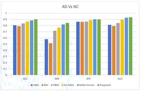
Figure 3.
AD classification performance of proposed ARE-PaLED on the AIBL dataset.
The proposed ARE-PaLED method consistently outperforms the competing methods in most evaluation metrics for AD classification when distinguishing them from NC. ADNI-trained models were used to classify AD vs. NC subjects in the AIBL dataset. The ARE-PaLED achieves an accuracy of 0.901, surpassing other approaches such as VBM (0.805), ROI (0.788), PLM (0.834), DMIL (0.863), and MAD-Former (0.884). This highlights its superior ability to identify AD patients accurately.
The findings further underline the robust performance of the proposed method across different datasets, demonstrating minimal performance degradation for the AD vs. NC classification compared to the results presented in Table 2. However, the proposed approach could not validate MCI classification with the AIBL dataset. This is attributed to the fact that there are no MCI samples in the AIBL dataset, where even a single misclassification significantly impacts sensitivity. Despite this challenge, the proposed approach maintains its strong generalisation capability, showcasing its effectiveness and reliability for AD diagnosis across datasets. These results emphasise the potential of the proposed ARE-PaLED method to be a valuable system for improving the identification of AD and related conditions.
MMSE-Driven Bias
In the AIBL dataset, a sharp separation is observed between the AD and NC groups in terms of MMSE scores (e.g., 20.23 ± 5.76 for AD and 28.65 ± 1.35 for NC). This pronounced gap can inadvertently simplify the classification task, leading models to rely on cognitive severity cues, such as global brain atrophy, rather than learning disease-specific structural features. MMSE-based stratification is applied during dataset construction to mitigate this bias. Specifically, subjects with extreme MMSE values (e.g., MMSE < 15 for AD or MMSE > 29 for NC) were excluded to eliminate outlier-driven classification that could be dominated by disease severity rather than neuroanatomical features.
The model’s reliance on image features rather than cognitive score extremes was validated empirically through a focused evaluation on a subset of subjects with closely matched MMSE scores. Despite the minimal difference in cognitive scores, the model accurately distinguished between AD and NC groups. The results, presented in Table 5, demonstrate that classification was not solely driven by cognitive metrics. ARE-PaLED successfully classified these cases despite the negligible MMSE gap. Figure 4 shows representative z-score activation maps for these subjects. The corresponding maps reveal strong activations in disease-relevant regions, highlighted in red, such as the medial temporal and parietal areas for the AD subject. In contrast, the NC subject exhibits minimal or non-specific activation. These findings underscore that the model’s predictions are primarily driven by sMRI features rather than cognitive assessments alone.
Table 5.
Representative samples with closely matched MMSE scores demonstrating that ARE-PaLED classification is primarily driven by sMRI features rather than cognitive score differences.
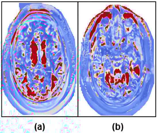
Figure 4.
Z-score maps highlighting disease-relevant anatomical regions for two subjects with closely matched MMSE scores. (a) AD subject with MMSE = 26.5. (b) NC subject with MMSE = 24.7. Red regions indicate high z-score values corresponding to model-identified discriminative brain areas. Despite similar cognitive performance, the model accurately differentiates these subjects based on structural features localised to disease-specific regions.
5.5. Comparison with XAI Models
Recent advances in XAI for AD diagnosis include several notable models. Each employs state-of-the-art interpretability techniques yet varies in terms of granularity, anatomical specificity, and classification performance. Ref. [61] propose a dual-model approach, utilising sMRI with ResNet-18 and diffusion-based BC-GCN-SE networks, and evaluate it through a novel parcel-wise Grad-CAM-based XAI metric over 132 cortical and subcortical regions, enabling alignment with known Alzheimer’s biomarkers. However, the method lacks sub-parcel resolution, limiting the ability to pinpoint fine-grained discriminative features within each brain region. Ref. [62] developed a 3D-ResNet with self-attention modules (SAM) trained on ADNI. They apply Grad-CAM to produce 3D saliency maps, identifying the hippocampus and cerebral cortex, but again, these remain volumetric heatmaps without intra-region granularity. Ref. [63] proposed a CNN-based framework utilizing VGG and DenseNet architectures trained on sMRI. They incorporated Grad-CAM for visualisation, highlighting brain regions associated with AD, such as the hippocampus and ventricles. Their approach focused on slice-level saliency maps, which, while informative, lacked sub-regional specificity.
In contrast, the ARE-PaLED framework proposed in this study introduces a novel, multi-modal explainability pipeline that operates at the patch level. By combining voxel-wise statistical analysis, gradient-based attribution, and evolutionary patch selection (IPSA), ARE-PaLED provides a highly granular and region specific interpretability mechanism. Unlike previous methods, it does not rely solely on full-slice or region-level saliency. Instead, it highlights functionally relevant subregions within anatomical structures, such as the hippocampus and frontal lobe.
All models were retrained and assessed using our curated ADNI dataset to ensure consistency in evaluation. The comparison highlights differences in classification performance as well as the granularity and depth of explainability offered by each method. Table 6 presents a comparative evaluation of recent state-of-the-art models alongside our proposed ARE-PaLED framework.
Table 6.
Comparison of model accuracy and explainability granularity.
Moreover, ARE-PaLED integrates AMPEN and IPSA for model-agnostic feature attribution and uniquely projects explanatory regions into an immersive AR environment, enabling real-time, browser-based visualization of affected patches. This interactive capability is absent in prior works. While [62] achieved slightly higher accuracy than the other two existing methods, their method lacks patch-level interpretability and interactivity. Ref. [61] offers biomarker-aware XAI via parcel-level Grad-CAM but without inter-patch analysis or spatial learning. Ref. [63] is limited to classic Grad-CAM without anatomical alignment or multi-resolution fusion.
Figure 5 illustrates the interpretability performance of various explainable AI methods applied to structural brain MRI for AD classification. Notably, the heat maps produced by the proposed ARE-PaLED framework (rightmost column) explicitly highlight disease-relevant brain regions, particularly those associated with atrophy such as the medial temporal lobe and hippocampus. These patches are identified by the AMPEN and IPSA of the proposed ARE-PaLED resulting in more focused and region specific visuals. Refs. [62,63] shows less localised saliency regions that lack precise anatomical alignment. This highlights ARE-PaLED’s capacity to identify and visualise disease-relevant regions linked to AD. Furthermore, expert review of the XAI outputs affirmed their interpretability and practical value in aiding clinical assessment.
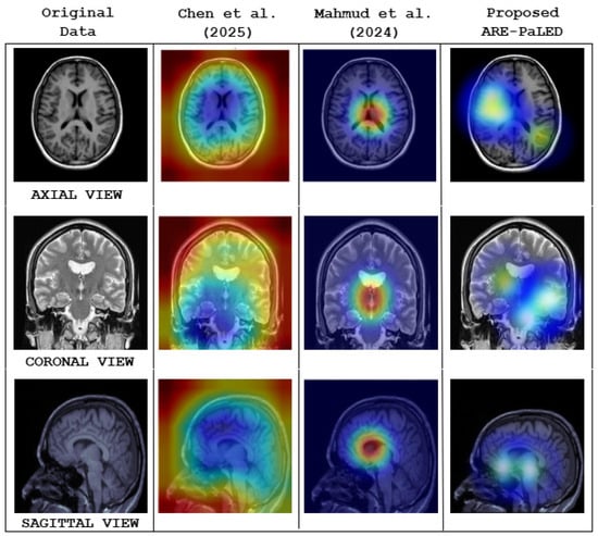
Figure 5.
Qualitative comparison of model interpretability across different explainable AI (XAI) methods using 3D structural brain MRI slices from axial, coronal, and sagittal views. The first column shows the original MRI scan of AD subject. The second and third columns visualise heat maps generated by the methods proposed by Chen et al. [62] and Mahmud et al. [63], respectively. The fourth column presents the heat maps generated by the proposed ARE-PaLED framework.
6. Discussion
This section discusses the key outcomes and insights derived from our study. First, a thorough evaluation of diagnostic performance is presented, using metrics such as accuracy, sensitivity, specificity, and area under the ROC curve to quantify ARE-PaLED’s ability to distinguish among AD, MCI, and NC subjects. Next, the distinctive regions of various brain symmetry highlighted by our framework are projected in AR for exploring their known roles in AD pathology and progression. Later, the result screenshot discussions include illustrations of the spatial distribution of informative patches across brain symmetry, as well as a discussion of the characteristics of individual patches that most strongly influenced classification decisions. Finally, the limitations of the proposed approach and the outline of future work are acknowledged.
6.1. Evaluation of Diagnostic Performance
These experiments used the year one ADNI-2 and ADNI-3 datasets as training and testing sets. Table 2, Table 3 and Table 4 present the performance of classification for AD versus NC, MCI versus NC, and AD versus MCI, respectively, using various competing methods (ROI, VBM, Patch-Based Method, DA-MIDL, and MAD-Former) and the proposed ARE-PaLED approach.
- All the competing patch-based methods [25] demonstrate superior classification compared to both ROI [15] and VBM [8] approaches. This highlights that the proposed ARE-PaLED, which adopts patch-level feature representations using multiscale patches, as a median measure between region and voxel-based features, can capture more indicative information about nuanced brain transformations, making it particularly effective for diagnosing AD.
- When VBM [8] and ROI [15] methods are compared, the VBM method yields better accuracy for both AD and MCI classification. Therefore, the improvement in classification accuracy of the proposed ARE-PaLED is also due to the efficient combination of VBM with the patch-based approach.
- Deep learning methods achieve more significant classification accuracy in all three classification tasks, as shown in Table 2, Table 3 and Table 4, than traditional machine learning approaches. This illustrates that using efficient feature engineering of deep learning using the patch-based method in the proposed ARE-PaLED improves its classification performance.
- The proposed ARE-PaLED demonstrates competitive performance in AD classification compared to leading-edge approaches such as DA-MIDL [34] and MAD-Former [58]. Moreover, it outperforms these methods in distinguishing MCI from AD and NC. This improved performance can be attributed to integrating VBM with GE, which combines statistical significance with structural information. This synergy enhances feature localisation, making the extracted features more robust and informative. In the next step, the most informative features are selected and classified using a unified deep-learning framework, aiming to enhance classification accuracy further.
Recent baseline models RV-ELSTSVM [59] and CAPsNET-3D [60] are evaluated for AD Vs CN, MCI Vs CN, and AD Vs MCI. Their performance accuracies (in Table 2, Table 3 and Table 4) are lower than those of the proposed model. The RV-ELSTSVM [59] utilises 2D sagittal slices, which limits its anatomical coverage due to the lack of 3D spatial context. It provides no interpretability or regional insight. Additionally, its hybrid SVM classifier does not support end-to-end learning, making it less adaptable than ARE-PaLED’s framework. The CAPsNET-3D [60] focuses solely on the hippocampal region, which limits its ability to capture disease-related changes across the whole brain. It lacks interpretability tools such as saliency or attention maps, offering no insight into decision-making. It does not support multi-scale analysis, unlike the proposed model.
6.2. Complexity and Transferability
The computational complexity of ARE-PaLED is primarily driven by its ViT-based classification module, which scales as , where P is the number of selected patches, H is the hidden size, and L is the number of transformer layers. Additional overhead is introduced by the VBM, GE, and IPSA modules during patch selection; however, these operations are performed only once per scan. Despite this added cost, the IPSA module effectively reduces redundant patches, thus helping manage overall computational demand.
We further evaluated the complexity and cross-dataset generalisation performance of ARE-PaLED in comparison with two state-of-the-art frameworks: MAD-Former [58] and DA-MIDL [34]. ARE-PaLED integrates additional architectural components, including a Fuse-Net fusion CNN, two 3D fully connected convolutional networks (FCNs) for VBM and gradient estimation, and an evolutionary IPSA. Consequently, its total parameter count is approximately , slightly higher than that of DA-MIDL () and MAD-Former ().
Notably, in cross-dataset evaluations, ARE-PaLED exhibits only a 2.4% drop in AD vs. NC classification accuracy, significantly outperforming DA-MIDL [34] (5.0%) and MAD-Former [58] (11.5%) under identical conditions. These results demonstrate that ARE-PaLED achieves superior generalisation to unseen data, offering a favorable trade-off between interpretability, computational complexity, and transferability.
6.3. Distinctive Brain Regions and Their Role in AD Diagnosis
Clinical application is a critical aspect of computer-assisted Alzheimer’s disease (AD) diagnosis. One essential factor in diagnosing AD is recognising structural alterations in the brain, particularly areas exhibiting abnormal shrinkage. The proposed ARE-PaLED framework supports this process by autonomously detecting potential disease-related regions across entire MRI scans, aiding clinicians in efficiently locating key areas for assessment. More specifically, our approach uses AR, which aids in uncovering patient-specific distinctive pathological sites, identifying broad regions of significance and subtle structural deviations within localised areas.
6.4. Informative Patch Locations
The last two rows of Figure 6 show the informative locations of patches in sMRI identified by AMPEN. The informative patch sites in 3D Brain MRI scans are visualised in axial, coronal, and sagittal views, with patches of varying sizes, demonstrating a strategic approach to capturing relevant brain structures. The results highlight that larger patch sizes (32 × 32 × 32) are extracted from the more informative locations, and smaller patches (16 × 16 × 16) are extracted in other brain areas, ensuring a more detailed local representation while maintaining computational efficiency. These patches are identified based on the z-score, which combines both VBM and GE, and they align with regions of interest such as the hippocampus, amygdala, and thalamus—areas consistently highlighted in previous studies [22,23,25] as crucial in AD research due to their involvement in neurodegeneration. Additionally, there is a considerable association between the two tasks concerning the course of AD, as seen by the high similarity of the likely problematic regions for AD and MCI categorisation.
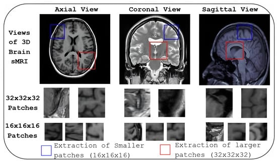
Figure 6.
Informative patch locations identified by AMPEN. Patch locations are visualised in three orthogonal views: axial, coronal, and sagittal. Patches of varying sizes, (32 × 32 × 32) and (16 × 16 × 16) are shown in the last two rows.
6.5. Information on Individual Patches
The region-specific contributions of brain areas relevant to AD and MCI, as projected in AR, are illustrated in Figure 7. The figure highlights the discriminative patches identified by the IPSA algorithm for both MCI and AD participants, with high IPSA-derived z-scores. These patches, overlaid on the axial view of sMRI, are visualised in AR to reflect the predicted diagnostic significance. For both MCI (Figure 7a) and AD (Figure 7b) cases, the most informative patches are emphasised in red, indicating a strong contribution to the classification task. Notably, these patches are predominantly located near the hippocampus, falx cerebri and in the cortical gray matter regions. Upon user interaction (tapping), metadata popups reveal the z-scores and the ARE-PaLED model’s predicted class labels (MCI or AD), enhancing interpretability. These highlighted regions suggest that localised structural alterations—particularly those indicative of cortical thinning and medial structural deformation—are closely associated with neurodegenerative atrophy patterns in AD and MCI.
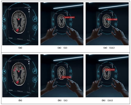
Figure 7.
Augmented reality–based patch-level explainability interface. (a,b) Interactive AR views of 3D brain MRI slices for MCI and AD cases, respectively, overlaid with informative patches selected via the IPSA algorithm. (ai,aii) Visually highlighted patches that, when tapped, activate metadata popups displaying IPSA-derived z-scores (1.4 and 1.2, respectively) and the proposed ARE-PaLED model’s predicted class label: MCI. (bi,bii) Visually highlighted patches that, when tapped, activate metadata popups displaying IPSA-derived z-scores (1.7 and 1.8, respectively) and the proposed ARE-PaLED model’s predicted class label: AD.
6.6. Empirical Support and Preliminary Validation
Preliminary empirical support for the practical applicability of our model is provided by an additional test that was conducted using a small set of previously unlabeled sMRI scans. These scans were retrospectively reviewed and labelled by qualified medical experts to establish reference diagnoses. The performance of ARE-PaLED was then evaluated on these expert-labelled cases using the same trained model without further fine-tuning. The model demonstrated consistent classification outcomes that aligned with expert labels in most cases, suggesting its generalisability to unseen data. Figure 8 demonstrates the empirical applicability and diagnostic consistency of the ARE-PaLED framework on previously unlabeled MRI data. The interpretability of the XAI outputs along with AR-based visualisations produced by ARE-PaLED was validated through expert review, with clinicians confirming their relevance and utility in supporting diagnostic decisions.
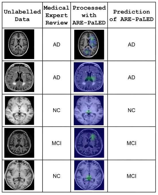
Figure 8.
Qualitative validation of ARE-PaLED on retrospectively annotated unlabeled MRI cases. Each row shows one subject. The first column displays original structural brain MRI slices (unlabeled at test time). The second column indicates the expert-determined diagnosis after retrospective review. The third column presents the heatmap output generated by ARE-PaLED, highlighting the regions that contribute to its prediction. The fourth column shows the corresponding model-predicted label. The model’s predictions align with expert review, and the highlighted regions demonstrate interpretability through localised atrophy patterns (e.g., in hippocampal and cortical regions).
6.7. Limitations and Future Work
The proposed ARE-PaLED method shows notable effectiveness in automatic discriminative localisation and brain disease diagnosis, especially in tasks related to AD. However, addressing specific challenges and limitations could improve its generalisation ability. Although the approach successfully identifies pathological regions and supports AD diagnosis, certain factors may affect its overall robustness. This section discusses these limitations and recommends strategies to enrich the model’s performance and tractability in future developments.
First, the current framework extracts non-overlapping patches of varying but predefined sizes from the 3D brain sMRI. While effective, this approach may overlook contextual or spatial relationships between adjacent patches. To address this, adaptive-sized patches with overlapping regions or dynamic scaling mechanisms could be introduced, improving the capture of fine-grained structural variations and spatial dependencies. Second, the IPSA evaluates patches individually based on their fitness. It may exclude less important but precious patches when combined with others. Future work could explore advanced patch evaluation strategies for more robust selection, including inter-patch relationships and suitable dependencies. Third, the framework is currently designed to process unimodal data (sMRI), limiting its ability to leverage corresponding information from other modalities. Extending the framework to a multimodal approach by incorporating data such as PET scans, genetic profiles, and clinical biomarkers could enhance diagnostic accuracy and robustness. Fourth, the method is tailored for cross-sectional data, overlooking temporal changes in brain structure. Incorporating longitudinal data analysis could enable the framework to track disease progression, monitor the transition from MCI to AD, and provide early intervention opportunities. Fifth, the global spatial mapping and classification steps operate as separate modules, possibly controlling the interaction between local and global features. A multi-task learning framework could unify these components, enabling the simultaneous optimisation of location proposals, feature extraction, and classification. Sixth, AR projections enhance interpretability, but their practical use in clinical workflows still needs to be explored. Future work could develop interactive tools that integrate these projections into clinical systems. Seventh, the proposed model’s generalisation is performed on the AIBL dataset, which includes only AD and NC subjects, and does not contain MCI cases. As a result, cross-dataset validation is performed for AD diagnosis only, not for early-stage diagnosis involving MCI. Future work could incorporate the MCI subgroup from OASIS-3 dataset and, through data augmentation, evaluate the model’s early diagnostic generalisation across different cohorts. Finally, the perspective of combining multi-task learning with multimodal data and longitudinal analysis could further elevate the framework’s capability. The model could widely understand disease progression by jointly analysing spatial, temporal, and multimodal information, paving the way for personalised and early-stage AD diagnosis.
7. Conclusions
In this study, we present ARE-PaLED, an AR-enabled framework for explainable deep learning aimed at supporting Alzheimer’s disease (AD) diagnosis using sMRI. The framework integrates voxel-level statistical analysis with a dynamic, patch-based approach to capture multi-scale neurodegenerative patterns associated with AD. It incorporates AMPEN, which leverages voxel-wise p-value maps and regional brain symmetry to adaptively extract informative patches, and IPSA, an evolutionary algorithm that selects non-redundant patches with high diagnostic relevance.
By incorporating asymmetry-aware analysis, ARE-PaLED is designed to be sensitive to the localised and asymmetric atrophy patterns often observed in early-stage AD. Furthermore, the integration of augmented reality (AR) enhances interpretability by providing an interactive and spatially grounded visualisation of the model’s predictions. The explainability outputs, including AR projections, have been reviewed by a medical expert, and they confirmed their alignment with clinically relevant brain regions for aiding decision making. The current results suggest that ARE-PaLED offers a balanced approach to diagnostic accuracy and interpretability, contributing to the advancement of explainable AI in neuroimaging applications.
Author Contributions
B.U. was responsible for conceptualisation, design of the methodology, software development, formal analysis, investigation, data curation, visualisation, and preparation of the original manuscript draft. C.S. contributed to the validation of results, provision of resources, manuscript review and editing, supervision, and overall project administration. All authors have read and agreed to the published version of the manuscript.
Funding
This research received no external funding.
Data Availability Statement
The data supporting the findings of this study are publicly available from the Alzheimer’s Disease Neuroimaging Initiative (ADNI) and the Australian Imaging, Biomarkers and Lifestyle (AIBL) study. These datasets comprise extensive multimodal imaging and clinical records of individuals diagnosed with Alzheimer’s disease. Interested researchers can apply for access via the ADNI website at (https://adni.loni.usc.edu) accessed on 20 March 2025. To request data, applicants must complete and submit the access form at (https://adni.loni.usc.edu/data-samples/adni-samples/#ApplyForAccessToSamples) accessed on 20 March 2025. Upon approval, credentialed users will be granted access to the datasets through the Image and Data Archive (IDA) portal at (https://ida.loni.usc.edu/login.jsp) accessed on 25 March 2025.
Acknowledgments
The authors express their sincere gratitude to the Department of Computer Science and Engineering, College of Engineering, Anna University, Guindy, Chennai, for providing the necessary support to carry out this research. This study used data from the Alzheimer’s Disease Neuroimaging Initiative (ADNI) database. The ADNI investigators were responsible for the design and implementation of the ADNI project but were not involved in the data analysis or the preparation of this manuscript.
Conflicts of Interest
The authors declare that they have no known competing financial interests or personal relationships that could have appeared to influence the work reported in this paper.
References
- Alzheimer’s Association. 2023 Alzheimer’s disease facts and figures. Alzheimer’s Dement. 2023, 19, 1598–1695. [Google Scholar] [CrossRef]
- Bharathi, U.; Chitrakala, S. Computer aided Alzheimer’s disease diagnosis from brain imaging dataset—A review. In Proceedings of the 2023 Intelligent Computing and Control Engineering in Business Systems (ICCEBS 2023), Chennai, India, 14–15 December 2023; pp. 1–6. [Google Scholar]
- Atri, A. Current and future treatments in Alzheimer’s disease. Semin. Neurol. 2019, 39, 227–240. [Google Scholar] [CrossRef]
- Vemuri, P.; Jack, C.R., Jr. Role of structural MRI in Alzheimer’s disease. Alzheimer’s Res. Ther. 2010, 2, 23. [Google Scholar] [CrossRef]
- Emmanuel, M.; Jabez, J. Classifying Alzheimer’s disease from sMRI data using a hybrid deep learning approach. Salud Cienc. Tecnol. Ser. Conf. 2024, 3, 651. [Google Scholar]
- Vounou, M.; Janousova, E.; Wolz, R.; Stein, J.L.; Thompson, P.M.; Rueckert, D.; Montana, G.; ADNI. Sparse reduced-rank regression detects genetic associations with voxel-wise longitudinal phenotypes in Alzheimer’s disease. NeuroImage 2012, 60, 700–716. [Google Scholar] [CrossRef] [PubMed]
- Baron, J.C.; Chételat, G.; Desgranges, B.; Perchey, G.; Landeau, B.; de la Sayette, V.; Eustache, F. In vivo mapping of gray matter loss with voxel-based morphometry in mild Alzheimer’s disease. NeuroImage 2001, 14, 298–309. [Google Scholar] [CrossRef] [PubMed]
- Ashburner, J.; Friston, K.J. Voxel-based morphometry—The methods. NeuroImage 2000, 11 (Pt 1), 805–821. [Google Scholar] [CrossRef]
- Liu, M.; Zhang, D.; Yap, P.T.; Shen, D. Tree-guided sparse coding for brain disease classification. In Lecture Notes in Computer Science (Including Subseries Lecture Notes in Artificial Intelligence and Lecture Notes in Bioinformatics); Springer: Berlin/Heidelberg, Germany, 2012; pp. 239–247. [Google Scholar]
- Cho, Y.; Seong, J.-K.; Jeong, Y.; Shin, S.Y.; ADNI. Individual subject classification for Alzheimer’s disease based on incremental learning using a spatial frequency representation of cortical thickness data. NeuroImage 2012, 59, 2217–2230. [Google Scholar] [CrossRef]
- Cuingnet, R.; Gerardin, E.; Tessieras, J.; Auzias, J.; Lehéricy, S.; Habert, M.O.; Chupin, M.; Benali, H.; Colliot, O. Automatic classification of patients with Alzheimer’s disease from structural MRI: A comparison of ten methods using the ADNI database. NeuroImage 2011, 56, 766–781. [Google Scholar] [CrossRef]
- Goenka, N.; Tiwari, S. AlzVNet: A volumetric convolutional neural network for multiclass classification of Alzheimer’s disease through multiple neuroimaging computational approaches. Biomed. Signal Process. Control 2022, 74, 103500. [Google Scholar] [CrossRef]
- Nanni, L.; Brahnam, S.; Salvatore, C.; Castiglioni, I. Texture descriptors and voxels for the early diagnosis of Alzheimer’s disease. Artif. Intell. Med. 2019, 97, 19–26. [Google Scholar] [CrossRef] [PubMed]
- Shao, W.; Peng, Y.; Zu, C.; Wang, M.; Zhang, D. Hypergraph based multi-task feature selection for multimodal classification of Alzheimer’s disease. Comput. Med. Imaging Graph. 2020, 80, 101663. [Google Scholar] [CrossRef] [PubMed]
- Zhang, D.; Wang, Y.; Zhou, L.; Yuan, H.; Shen, D. Multimodal classification of Alzheimer’s disease and mild cognitive impairment. NeuroImage 2011, 55, 856–867. [Google Scholar] [CrossRef]
- Zhang, D.; Shen, D. Multi-modal multi-task learning for joint prediction of multiple regression and classification variables in Alzheimer’s disease. NeuroImage 2012, 59, 895–907. [Google Scholar] [CrossRef]
- Cao, P.; Liu, X.; Yang, J.; Zhao, D.; Huang, M.; Zhang, J.; Zaiane, O. Nonlinearity-aware based dimensionality reduction and over-sampling for AD/MCI classification from MRI measures. Comput. Biol. Med. 2017, 91, 21–37. [Google Scholar] [CrossRef]
- Liu, Y.; Mazumdar, S.; Bath, P.A. An unsupervised learning approach to diagnosing Alzheimer’s disease using brain magnetic resonance imaging scans. Int. J. Med. Inform. 2023, 173, 105054. [Google Scholar] [CrossRef]
- Lian, C.; Liu, M.; Pan, Y.; Shen, D. Attention-guided hybrid network for dementia diagnosis with structural MR images. IEEE Trans. Cybern. 2022, 52, 1992–2003. [Google Scholar] [CrossRef] [PubMed]
- Liu, J.; Li, M.; Lan, W.; Wu, F.X.; Pan, Y.; Wang, J. Classification of Alzheimer’s disease using whole brain hierarchical network. IEEE/ACM Trans. Comput. Biol. Bioinform. 2018, 15, 624–632. [Google Scholar] [CrossRef]
- Zeng, N.; Qiu, H.; Wang, Z.; Liu, W.; Zhang, H.; Li, Y. A new switching-delayed-PSO-based optimized SVM algorithm for diagnosis of Alzheimer’s disease. Neurocomputing 2018, 320, 195–202. [Google Scholar] [CrossRef]
- Zhang, J.; Liu, M.; An, L.; Gao, Y.; Shen, D. Alzheimer’s disease diagnosis using landmark-based features from longitudinal structural MR images. IEEE J. Biomed. Health Inform. 2017, 21, 1607–1616. [Google Scholar] [CrossRef]
- Lian, C.; Liu, M.; Zhang, J.; Shen, D. Hierarchical fully convolutional network for joint atrophy localization and Alzheimer’s disease diagnosis using structural MRI. IEEE Trans. Pattern Anal. Mach. Intell. 2020, 42, 880–893. [Google Scholar] [CrossRef]
- Tong, T.; Wolz, R.; Gao, Q.; Guerrero, R.; Hajnal, J.V.; Rueckert, D. Multiple instance learning for classification of dementia in brain MRI. Med. Image Anal. 2014, 18, 808–818. [Google Scholar] [CrossRef]
- Zhang, J.; Gao, Y.; Gao, Y.; Munsell, B.C.; Shen, D. Detecting anatomical landmarks for fast Alzheimer’s disease diagnosis. IEEE Trans. Med. Imaging 2016, 35, 2524–2533. [Google Scholar] [CrossRef]
- Liu, M.; Zhang, D.; Yap, P.T.; Shen, D. Hierarchical ensemble of multi-level classifiers for diagnosis of Alzheimer’s disease. In Lecture Notes in Computer Science (Including Subseries Lecture Notes in Artificial Intelligence and Lecture Notes in Bioinformatics); Springer: Berlin/Heidelberg, Germany, 2012; pp. 27–35. [Google Scholar] [CrossRef]
- Liu, M.; Zhang, D.; Shen, D. ADNI. Ensemble sparse classification of Alzheimer’s disease. NeuroImage 2012, 60, 1106–1116. [Google Scholar] [CrossRef]
- Qiu, S.; Joshi, P.S.; Miller, M.I.; Xue, C.; Zhou, X.; Karjadi, C.; Chang, G.H.; Joshi, A.S.; Dwyer, B.; Zhu, S.; et al. Development and validation of an interpretable deep learning framework for Alzheimer’s disease classification. Brain 2020, 143, 1920–1933. [Google Scholar] [CrossRef] [PubMed]
- Zhang, X.; Han, L.; Han, L.; Chen, H.; Dancey, D.; Zhang, D. sMRI-PatchNet: A novel efficient explainable patch-based deep learning network for Alzheimer’s disease diagnosis with structural MRI. IEEE Access 2023, 11, 108603–108616. [Google Scholar] [CrossRef]
- Mendoza-Léon, R.; Puentes, J.; Uriza, L.F.; Hoyos, M.H. Single-slice Alzheimer’s disease classification and disease regional analysis with supervised switching autoencoders. Comput. Biol. Med. 2020, 116, 103534. [Google Scholar] [CrossRef] [PubMed]
- Zhang, J.; Zheng, B.; Gao, A.; Feng, X.; Liang, D.; Long, X. A 3D densely connected convolution neural network with connection-wise attention mechanism for Alzheimer’s disease classification. Magn. Reson. Imaging 2021, 78, 119–126. [Google Scholar] [CrossRef]
- Sushmitha, S.; Chitrakala, S.; Bharathi, U. sMRI classification of Alzheimer’s disease using genetic algorithm and multi-instance learning (GA + MIL). In Proceedings of the IEEE International Conference on Electrical, Electronics, Communication and Computer Engineering (ELEXCOM), Roorkee, India, 26–27 August 2023; pp. 1–4. [Google Scholar] [CrossRef]
- Ashtari-Majlan, M.; Seifi, A.; Dehshibi, M.M. A multi-stream convolutional neural network for classification of progressive MCI in Alzheimer’s disease using structural MRI images. IEEE J. Biomed. Health Inform. 2022, 26, 3918–3926. [Google Scholar] [CrossRef]
- Zhu, W.; Sun, L.; Huang, J.; Han, L.; Zhang, D. Dual attention multi-instance deep learning for Alzheimer’s disease diagnosis with structural MRI. IEEE Trans. Med. Imaging 2021, 40, 2354–2366. [Google Scholar] [CrossRef]
- Sánchez-Reyna, A.G.; Celaya-Padilla, J.M.; Galván-Tejada, C.E.; Luna-García, H.; Gamboa-Rosales, H.; Ramírez-Morales, A.; Galván-Tejada, J.I.; Alzheimer’s Disease Neuroimaging Initiative. Multimodal early Alzheimer’s detection, a genetic algorithm approach with support vector machines. Healthcare 2021, 9, 971. [Google Scholar] [CrossRef]
- García-Gutierrez, F.; Díaz-Álvarez, J.; Matias-Guiu, J.A.; Pytel, V.; Matías-Guiu, J.; Martín, M.N.; Ayala, J. GA-MADRID: Design and validation of a machine learning tool for the diagnosis of Alzheimer’s disease and frontotemporal dementia using genetic algorithms. Med. Biol. Eng. Comput. 2022, 60, 2737–2756. [Google Scholar] [CrossRef] [PubMed]
- Goel, T.; Sharma, R.; Tanveer, M.; Suganthan, P.N.; Maji, K.; Pilli, R. Multimodal neuroimaging based Alzheimer’s disease diagnosis using evolutionary RVFL classifier. IEEE J. Biomed. Health Inform. 2023, 29, 3833–3841. [Google Scholar] [CrossRef] [PubMed]
- Díaz-Álvarez, J.; Matias-Guiu, J.A.; Cabrera-Martín, M.N.; Pytel, V.; Segovia-Ríos, I.; García-Gutiérrez, F.; Hernández-Lorenzo, L.; Matias-Guiu, J.; Carreras, J.L.; Ayala, J.L.; et al. Genetic algorithms for optimized diagnosis of Alzheimer’s disease and frontotemporal dementia using fluorodeoxyglucose positron emission tomography imaging. Front. Aging Neurosci. 2022, 13, 825233. [Google Scholar] [CrossRef]
- Xiao, Z.; Zhang, Y.; Deng, Z.; Liu, F. Light3DHS: A lightweight 3D hippocampus segmentation method using multiscale convolution attention and vision transformer. Neuroimage 2024, 292, 120608. [Google Scholar] [CrossRef] [PubMed]
- Bravo-Ortiz, M.A.; Guevara-Navarro, E.; Holguín-García, S.A.; Rivera-Garcia, M.; Cardona-Morales, O.; Ruz, G.A.; Tabares-Soto, R. SpectroCVT-Net: A convolutional vision transformer architecture and channel attention for classifying Alzheimer’s disease using spectrograms. Comput. Biol. Med. 2024, 181, 109022. [Google Scholar] [CrossRef]
- Khatri, U.; Kwon, G. Training vision transformer with gradient centralization optimizer for Alzheimer’s disease small dataset increase the diagnostic accuracy. TechRxiv. 2024. [Google Scholar] [CrossRef]
- Yu, Q.; Ma, Q.; Da, L.; Li, J.; Wang, M.; Xu, A.; Li, Z.; Li, W. A transformer-based unified multimodal framework for Alzheimer’s disease assessment. Comput. Biol. Med. 2024, 180, 105495. [Google Scholar] [CrossRef]
- Almufareh, M.F.; Tehsin, S.; Humayun, M. Artificial cognition for detection of mental disability: A vision transformer approach for Alzheimer’s disease. Healthcare 2023, 11, 2763. [Google Scholar] [CrossRef]
- Akan, T.; Alp, S.; Bhuiyan, M.A.N. Vision transformers and Bi-LSTM for Alzheimer’s disease diagnosis from 3D MRI. In Proceedings of the 2023 Congress on Computational Science, Computational Engineering, and Applied Computing (CSCE 2023), Las Vegas, NV, USA, 24–27 July 2023; pp. 530–535. [Google Scholar] [CrossRef]
- Yu, L.; Xiang, W.; Fang, J.; Chen, Y.P.P.; Zhu, R. A novel explainable neural network for Alzheimer’s disease diagnosis. Pattern Recognit. 2022, 131, 108927. [Google Scholar] [CrossRef]
- Zhang, X.; Han, L.; Zhu, W.; Sun, L.; Zhang, D. An explainable 3D residual self-attention deep neural network for joint atrophy localization and Alzheimer’s disease diagnosis using structural MRI. IEEE J. Biomed. Health Inform. 2022, 26, 5289–5297. [Google Scholar] [CrossRef]
- Zhang, H.; Ni, M.; Yang, Y.; Xie, F.; Wang, W.; He, Y.; Chen, W.; Chen, Z. Patch-based interpretable deep learning framework for Alzheimer’s disease diagnosis using multimodal data. Biomed. Signal Process. Control 2025, 100, 107085. [Google Scholar] [CrossRef]
- Tekkesinoglu, S.; Pudas, S. Explaining graph convolutional network predictions for clinicians—An explainable AI approach to Alzheimer’s disease classification. Front. Artif. Intell. 2023, 6, 1141903. [Google Scholar] [CrossRef]
- Jahan, S.; Taher, K.A.; Kaiser, M.S.; Mahmud, M.; Rahman, M.S.; Hosen, A.S.M.S.; Ra, I.H. Explainable AI-based Alzheimer’s prediction and management using multimodal data. PLoS ONE 2023, 18, e0296536. [Google Scholar] [CrossRef] [PubMed]
- Kamal, M.S.; Northcote, A.; Chowdhury, L.; Dey, N.; Crespo, R.G.; Herrera-Viedma, E. Alzheimer’s patient analysis using image and gene expression data and explainable-AI to present associated genes. IEEE Trans. Instrum. Meas. 2021, 70, 2513107. [Google Scholar] [CrossRef]
- Bazargani, J.S.; Rahim, N.; Sadeghi-Niaraki, A.; Abuhmed, T.; Song, H.; Choi, S.M. Alzheimer’s disease diagnosis in the metaverse. Comput. Methods Programs Biomed. 2024, 255, 108348. [Google Scholar] [CrossRef]
- Słyk, S.; Zarzycki, M.Z.; Kocwa-Karnaś, A. Virtual reality in the diagnostics and therapy of neurological diseases. Expert Rev. Med. Devices 2019, 16, 1035–1040. [Google Scholar] [CrossRef] [PubMed]
- Riva, G.; Mancuso, V.; Cavedoni, S.; Stramba-Badiale, C. Virtual reality in neurorehabilitation: A review of its effects on multiple cognitive domains. Expert Rev. Med. Devices 2020, 17, 1035–1062. [Google Scholar] [CrossRef]
- González Izard, S.; Juanes Méndez, J.A.; Palomera, P.R.; Garcia-Penalvo, F.J. Applications of virtual and augmented reality in biomedical imaging. J. Med. Syst. 2019, 43, 68. [Google Scholar] [CrossRef]
- Bergonzi, L.; Colombo, G.; Redaelli, D.F.; Lorusso, M. An augmented reality approach to visualize biomedical images. Comput. Appl. Eng. Educ. 2019, 16, 1195–1208. [Google Scholar] [CrossRef]
- Benbelkacem, S.; Oulefki, A.; Agaian, S.; Zenati-Henda, N.; Trongtirakul, T.; Aouam, D.; Masmoudi, M.; Zemmouri, M. COVI3D: Automatic COVID-19 CT image-based classification and visualization platform utilizing virtual and augmented reality technologies. Diagnostics 2022, 12, 649. [Google Scholar] [CrossRef] [PubMed]
- Shen, D.; Davatzikos, C. HAMMER: Hierarchical attribute matching mechanism for elastic registration. IEEE Trans. Med. Imaging 2002, 21, 1421–1439. [Google Scholar] [CrossRef] [PubMed]
- Ye, J.; Zeng, A.; Pan, D.; Zhang, Y.; Zhao, J.; Chen, Q.; Liu, Y. MAD-Former: A traceable interpretability model for Alzheimer’s disease recognition based on multi-patch attention. IEEE J. Biomed. Health Inform. 2024, 28, 3637–3648. [Google Scholar] [CrossRef]
- Kumar, M.; Kumar, B.; Sharma, P.; Sharma, R.; Al-Dhaifallah, M.; Shakoor, A. Attentive deep learning with Randomized Vector Energy Least Square Twin Support Vector Machine for Alzheimer’s Disease diagnosis. Comput. Electr. Eng. 2025, 126, 110412. [Google Scholar] [CrossRef]
- Rasheed, J.; Shaikh, M.U.; Jafri, M.; Khan, A.U.; Sandhu, M.; Shin, H. Leveraging CapsNet for enhanced classification of 3D MRI images for Alzheimer’s diagnosis. Biomed. Signal Process. Control 2025, 103, 107384. [Google Scholar] [CrossRef]
- Coluzzi, D.; Bordin, V.; Rivolta, M.W.; Fortel, I.; Zhan, L.; Leow, A.; Baselli, G. Biomarker investigation using multiple brain measures from MRI through explainable artificial intelligence in Alzheimer’s disease classification. Bioengineering 2025, 12, 82. [Google Scholar] [CrossRef]
- Chen, D.; Yang, H.; Li, H.; He, X.; Mu, H. MRI-based diagnostic model for Alzheimer’s disease using 3D-ResNet. Biomed. Phys. Eng. Express 2025, 11, 035031. [Google Scholar] [CrossRef]
- Mahmud, T.; Barua, K.; Habiba, S.U.; Sharmen, N.; Hossain, M.S.; Andersson, K. An explainable AI paradigm for Alzheimer’s diagnosis using deep transfer learning. Diagnostics 2024, 14, 345. [Google Scholar] [CrossRef]
Disclaimer/Publisher’s Note: The statements, opinions and data contained in all publications are solely those of the individual author(s) and contributor(s) and not of MDPI and/or the editor(s). MDPI and/or the editor(s) disclaim responsibility for any injury to people or property resulting from any ideas, methods, instructions or products referred to in the content. |
© 2025 by the authors. Licensee MDPI, Basel, Switzerland. This article is an open access article distributed under the terms and conditions of the Creative Commons Attribution (CC BY) license (https://creativecommons.org/licenses/by/4.0/).