WaveAtten: A Symmetry-Aware Sparse-Attention Framework for Non-Stationary Vibration Signal Processing

Abstract

This study addresses the long-standing difficulty of predicting the remaining useful life (RUL) of rolling bearings from highly non-stationary vibration signals by proposing WaveAtten, a symmetry-aware deep learning framework. First, mirror-symmetric and bi-orthogonal Daubechies wavelet filters are applied to decompose each raw signal into multi-scale approximation/detail pairs, explicitly preserving the left–right symmetry that characterizes periodic mechanical responses while isolating asymmetric transient faults. Next, a bidirectional sparse-attention module reinforces this structural symmetry by selecting query–key pairs in a forward/backward balanced fashion, allowing the network to weight homologous spectral patterns and suppress non-symmetric noise. Finally, the symmetry-enhanced features—augmented with temperature and other auxiliary sensor data—are fed into a long short-term memory (LSTM) network that models the symmetric progression of degradation over time. Experiments on the IEEE PHM2012 bearing dataset showed that WaveAtten achieved superior mean squared error, mean absolute error, and R² scores compared with both classical signal-processing pipelines and state-of-the-art deep models, while ablation revealed a 6–8% performance drop when the symmetry-oriented components were removed. By systematically exploiting the intrinsic symmetry of vibration phenomena, WaveAtten offers a robust and efficient route to RUL prediction, paving the way for intelligent, condition-based maintenance of industrial machinery.

1. Introduction

Accurately predicting the remaining useful life (RUL) of equipment is a critical issue in the field of Prognostics and Health Management (PHM), as well as a challenging task [1]. Rolling bearings, as key components in rotating machinery, play a vital role in ensuring the overall normal operation and reliability of equipment [2]. Statistically, rolling bearing failures account for nearly 50% of common faults in rotating machinery. Therefore, effective RUL prediction for bearings enables more rational determination of maintenance and replacement schedules, ensuring optimal equipment utilization while maintaining safe and reliable operation, thus preventing economic losses and safety accidents. In recent years, with the rapid development of artificial intelligence, data-driven methods, particularly deep learning, have become the research focus in the PHM field. However, the community still lacks a consensus on how to simultaneously capture multi-scale degradation patterns and suppress redundant noise while keeping the model lightweight and interpretable—an open gap that motivates this study.

In the field of bearing RUL prediction, many researchers have proposed various predictive methods. Alfarizi et al. [1] predicted the RUL of experimental bearings by optimizing the random forest model, demonstrating the potential of machine learning in bearing life prediction. Cheng et al. [2] proposed an RUL prediction method combining dynamic models and transfer learning, offering new insights for dealing with data scarcity in real-world industrial applications. Cui et al. [3] used digital twin technology and graph domain adaptation neural networks to predict the RUL of rolling bearings, showcasing the advantages of this approach when handling cross-device data. Ding et al. [4] predicted the RUL of rolling bearings based on dilated causal convolutional dense networks and exponential models, demonstrating strong capabilities in handling time-series data. Dong et al. [5] and Xingjun et al. [6] used deep transfer learning and multi-constrained domain adaptation networks, respectively, for bearing RUL prediction, highlighting the effectiveness of deep learning in managing complex industrial data. Gupta et al. [7] introduced a real-time adaptive model using deep neural networks for bearing fault classification and RUL estimation, providing a new direction for real-time monitoring and prediction. Hou et al. [8] predicted bearing RUL under varying operating conditions using a cross-transformer fusion method with segmented data cleaning, which is innovative in handling non-stationary data. Kumar et al. [9] proposed an intelligent framework for monitoring bearing degradation, defect identification, and RUL estimation, which is advantageous for integrating multiple sensor data. Li et al. [10] and Yajing et al. [11], respectively, proposed RUL prediction methods based on implicit Kalman filtering and integrated data fusion, demonstrating innovations in adaptive degradation stage detection and data fusion. Lu et al. [12] predicted the RUL of cross-machine rolling bearings using enhanced residual convolutional domain adaptation networks, exhibiting better adaptability when handling cross-domain data. Mao et al. [13] introduced a self-supervised deep domain-adversarial regression adaptation method for online RUL prediction, showing promising performance under unknown operating conditions. Niazi et al. [14] utilized TT-ConvLSTM techniques to analyze multi-scale time-series data for bearing RUL prediction, highlighting its advantages in processing multi-scale data. Qi et al. [15] and Qiu [16] proposed RUL prediction methods based on anomaly detection and multi-step estimation, as well as time-convolutional network-based RUL estimation, respectively, contributing to improved prediction accuracy. Ren et al. [17] proposed a lightweight adaptive knowledge distillation framework for RUL prediction, offering innovations in model compression and optimization. Wang et al. [18] and Xiaokang et al. [19], respectively, introduced RUL prediction models based on Bayesian large-kernel attention networks and tensor-based t-SVD-LSTM, which are significant for uncertainty quantification and industrial intelligence. Wei et al. [20,21,22] proposed RUL prediction methods based on adaptive graph convolutional networks and conditional variational transformers, showing advantages in handling graph-structured data and cross-domain issues. Xiang et al. [23] proposed a concise self-adaptive deep learning network for machine RUL prediction, offering innovations in model simplification and adaptability. Xie et al. [24] introduced a multidimensional attention domain adaptation method combined with degradation priors for machine RUL prediction, which has advantages in handling multidimensional data and domain adaptation issues. Zhang et al. [25,26,27] proposed unsupervised learning models for health indicators, deep transfer learning, and two-stage data-driven methods for RUL prediction of rolling bearings, offering innovations in predicting different degradation stages and handling online prediction under unknown conditions. Zhang et al. [28] proposed a variational local weighted deep subdomain adaptation network for cross-domain RUL prediction, demonstrating better adaptability in addressing cross-domain issues. Zhou et al. [29] predicted RUL through distribution contact ratios, health indicators, and integrated memory GRU, offering innovative approaches to handling distributed data and memory-related issues. Zhuang et al. [30] introduced a multi-source adversarial online regression method for online bearing RUL prediction under unknown conditions, which provides advantages in handling multi-source data and online learning challenges.

Although wavelet transforms have been incorporated into deep learning models in domains such as wind speed prediction [31] and speech recognition [32], their application in non-stationary bearing vibration signals for remaining useful life (RUL) prediction remains relatively limited. Most existing studies either treat wavelet transform merely as a preprocessing or denoising step or fail to integrate it effectively with learnable attention mechanisms—particularly sparse-attention mechanisms suited for handling noise and redundancy in industrial non-stationary data. Furthermore, despite the growing number of methods proposed for bearing RUL prediction, key limitations remain. Many rely on shallow or fixed feature extractors, neglecting the adaptive multi-scale nature of degradation, attention mechanisms, while employed, are often dense and computationally demanding, and multi-sensor data fusion is usually ad hoc, lacking a principled approach to weighting different sources dynamically.

To address the above gaps, the primary objective of this study is to develop WaveAtten, an end-to-end framework that unifies wavelet-based decomposition, sparse-attention-driven feature selection, and LSTM-based temporal modeling for accurate and interpretable RUL prediction of rolling bearings. WaveAtten is designed to (i) preserve multi-resolution trend and anomaly features via discrete wavelet transform, (ii) leverage sparse attention to highlight degradation-relevant features while suppressing redundant noise, and (iii) seamlessly fuse auxiliary sensor channels through learnable weighting, thereby enabling dynamic cross-modal perception.

The proposed method exhibits several strengths: it offers an interpretable multi-scale representation, reduces computational overhead by employing sparsity, and naturally supports multi-sensor fusion in a single architecture. Nevertheless, it also has limitations. Contemporary data-driven RUL prediction models frequently underperform in real-world industrial settings for four principal reasons. First, domain shift: most models are trained on single-rig test beds or public benchmarks and thus struggle to generalize when confronted with distributional changes induced by varying loads, harsh environments, or manufacturing heterogeneity. Second, weak and highly non-stationary degradation signals: early-stage fault signatures are often buried in heavy noise and exhibit time-varying, nonlinear dynamics that fixed-window CNNs/LSTMs fail to capture. Third, label scarcity and uncertainty: true failure timestamps are rarely available at scale, and health labels are typically inferred heuristically or back-calculated from residual life, introducing substantial noise that causes supervised models to overfit. Fourth, absence of physics priors and multi-modal fusion: prevailing approaches seldom embed bearing dynamics or lubrication physics into the learning process and often rely on a single sensing modality (e.g., vibration), resulting in predictions that lack both interpretability and robustness. These factors jointly explain why existing RUL models still suffer from large errors and poor stability, especially in cross-domain deployment, early-warning scenarios, and noisy environments.

In essence, the unique contribution of this work lies in bridging traditional signal-processing insight (wavelet analysis) with modern sparse-attention networks to form a holistic, interpretable, and computationally efficient PHM solution for non-stationary bearing signals—something not yet achieved by the studies surveyed above.

WaveAtten not only preserves trend and anomaly features at different resolutions through wavelet transform but also adaptively highlights degradation-relevant features via sparse attention, while integrating auxiliary sensor data to enhance multi-modal perception and RUL prediction accuracy. Compared with previous methods, the proposed framework offers a systematic and interpretable mechanism for extracting, refining, and correlating features in complex industrial scenarios.

2. Problem Description

Given a time-series of multivariate sensor signals collected from rolling bearings under operating conditions, the goal is to predict the remaining useful life (RUL) of each bearing instance based on its historical degradation pattern. Let $X=\{x_1,x_2,\dots ,x_T\}\in {\mathbb{R}}^{T\times d}$ denote the sequence of sensor observations, where $T$ is the sequence length and $d$ is the number of sensor modalities, while $x_t\in {\mathbb{R}}^d$ represents the multivariate signal vector at time $t$ and $y\in \mathbb{R}$ denotes the scalar target value corresponding to the true RUL.

The objective is to learn a mapping function $f_{\theta }:{\mathbb{R}}^{T\times d}\to \mathbb{R}$, parameterized by deep neural network weights $\theta$, that minimizes the discrepancy between the predicted RUL $\hat{y}=f_{\theta }\left(X\right)$ and the true RUL $y$.

Formally, the learning objective is:

$$\underset{\theta }{min}{\mathbb{E}}_{(X,y)\sim \mathcal{D}}[\mathcal{L}(f_{\theta }(X),y)],$$

where $\mathcal{D}$ is the training data distribution and $\mathcal{L}$ is a regression loss function, such as mean squared error (MSE):

$${\mathcal{L}}_{\mathrm{M}\mathrm{S}\mathrm{E}}(\hat{y},y)={\displaystyle \frac{1}{n}}{\sum }_{i=1}^n({\hat{y}}_i-y_i{)}^2.$$

To address the challenges posed by non-stationary signals, multi-source sensor fusion, and early fault detection, the proposed model $f_{\theta }$ integrates wavelet-based signal decomposition, sparse attention for feature selection, and temporal modeling via LSTM.

3. WaveAtten Model Construction

3.1. Dataset

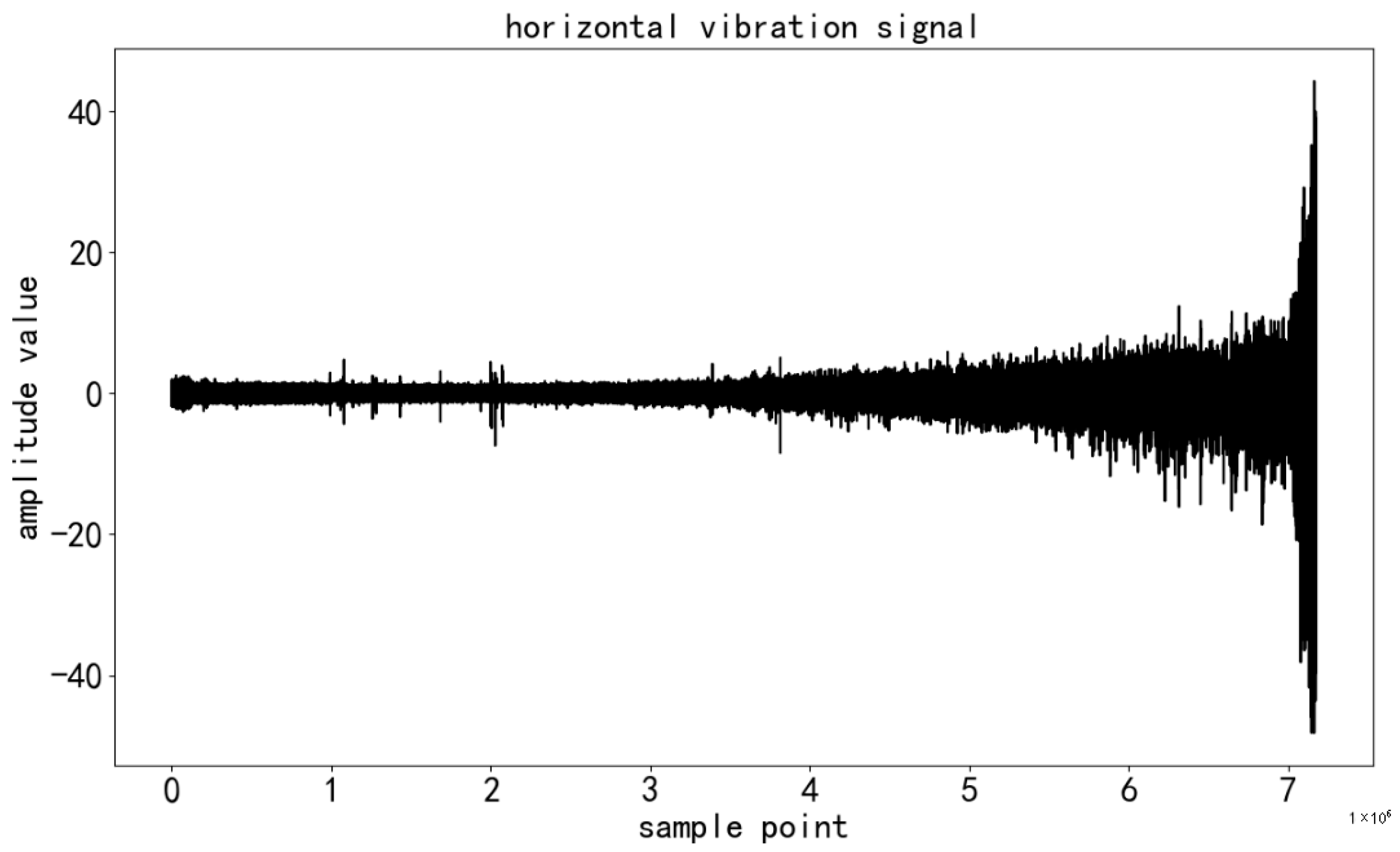
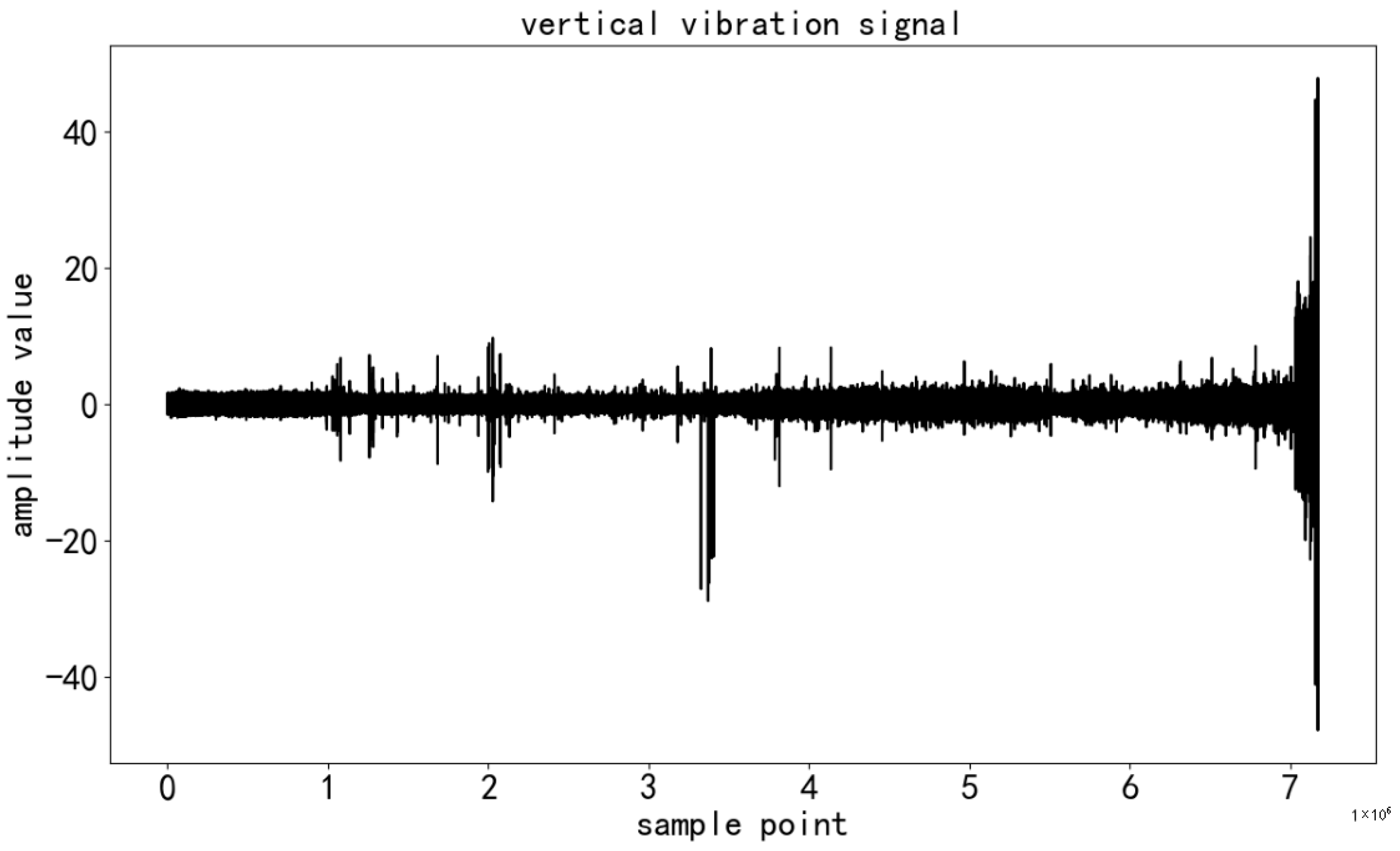
The PHM2012 dataset is an authoritative dataset provided by the IEEE Reliability Society and the FEMTO-ST Institute, as part of the IEEE PHM 2012 Data Challenge [33]. It is widely used in the field of bearing remaining useful life (RUL) prediction research and is highly representative. The dataset originates from a laboratory experimental platform (PRONOSTIA), and the experimental process is rigorous and controllable. The rotating part of the experimental platform is driven by a 250 W motor, with a maximum speed of 2830 rpm, ensuring that the second shaft remains stable at 2000 rpm, providing stable rotational conditions for the bearing. The load part uses a pneumatic jack to apply a dynamic load of 4000 N on the bearing, simulating the stress conditions encountered in actual industrial scenarios. The measurement part is equipped with high-precision sensors to collect various types of data during the bearing’s operation. The dataset includes vibration and temperature data. The vibration data are collected by two miniature accelerometers, positioned at a 90° angle to each other, capturing vibration information along the horizontal axis (Figure 1) and the vertical axis (Figure 2). With a sampling frequency of up to 25.6 kHz, the data can reflect the bearing’s vibration characteristics in the high-frequency range, which is crucial for capturing subtle fault impact signals during the early stages of bearing degradation.

From the perspective of the data organization structure, the dataset was divided into three folders: the learning set (Learning_set), the test set (Test_set), and the full-life set (Full_Test_set). The learning set was used for the initial training of the model and contained samples of bearings at various degradation stages, enabling the model to learn different feature patterns from the bearing’s initial healthy state to its gradual degradation. The test set consisted of truncated data used during the competition for evaluating the model’s predictive performance in real-world applications. The data distribution of the test set was similar to data typically observed in industrial settings, representing a stage before the occurrence of failure. This allowed for effective testing of the model’s generalization ability and prediction accuracy. The full-life set was the complete version of the test set, covering the entire lifecycle of the bearing from brand new to complete failure.

In terms of sample quantity, taking the vibration data files in the bearing_1–2 folder as an example (as shown in

Table 1. Sample of vibration data.

Hour	Minute	Second	μ-Second	Horizontal Acceleration	Vertical Acceleration
8	47	5	1.97 × 105	0.05	−0.253
8	47	5	1.97 × 105	0.165	−0.14
8	47	5	1.97 × 105	0.125	0.542
8	47	5	1.97 × 105	0.157	−0.261
8	47	5	1.97 × 105	0.421	0.081

), there were a total of 871. csv files. Each file recorded 2560 data points sampled within 0.1 s. The sample quantity was sufficient, providing a comprehensive reflection of the bearing’s operating conditions and degradation stages under different working conditions, which supported model training.

The temperature data (as shown in

Table 2. Sample of temperature data.

Hour	Minute	Second	0.x Second	RTD Sensor
8	9	47	9	70.036
8	9	48	0	70.036
8	9	48	1	70.058
8	9	48	2	70.058

) were collected by a resistance temperature detector (RTD). The detector was placed in a hole near the outer bearing ring, enabling real-time monitoring of the bearing’s operating temperature. The sampling frequency was 0.1 Hz, which is relatively low but sufficient to capture the temperature variation trend of the bearing over long periods of operation. These data provided a basis for assessing the bearing’s lubrication condition, wear-induced heating, and other related factors.

The PHM2012 dataset presents several unique characteristics and application challenges. On one hand, the vibration signals in the dataset exhibited typical non-stationarity. This is due to the various factors that influence the bearing during operation, including external load variations, speed fluctuations, changes in lubrication conditions, wear, and the initiation of fatigue cracks. These factors cause changes in frequency components, amplitude, phase, and other signal features over time, increasing the difficulty of signal analysis and feature extraction. On the other hand, there were differences in the sample distribution under different operating conditions. For instance, operating conditions 1 and 2 differed from condition 3 in terms of bearing load characteristics, operating duration, and fault types. Additionally, there was inconsistency in the number of samples and data feature distributions between the training and testing datasets for each operating condition. This raised higher requirements for the model’s generalization ability, necessitating the model to adaptively learn the bearing degradation features under various conditions. It is crucial to avoid overfitting to a specific condition and ensure accurate RUL predictions across different industrial scenarios.

To enhance the data quality and improve model training effectiveness, multidimensional preprocessing of the raw data is essential.

3.2. Preprocessing

Two complementary strategies were applied. First, a Hampel filter with a window size of nine samples (≈0.35 ms at 25.6 kHz) and a cutoff of 3 × MAD (median absolute deviation) was used to suppress impulsive spikes caused by electromagnetic interference. Any point whose absolute deviation from the local median exceeded this threshold was replaced by the median of its window. Second, a global 3σ criterion was enforced to discard sustained amplitude drifts that exceeded the mechanical specifications of the test rig: samples whose z-score |x − μ|/σ > 3 were removed and linearly interpolated. Empirically, <0.4% of the data was affected, preventing the deletion of genuine early-fault impulses while eliminating implausible excursions.

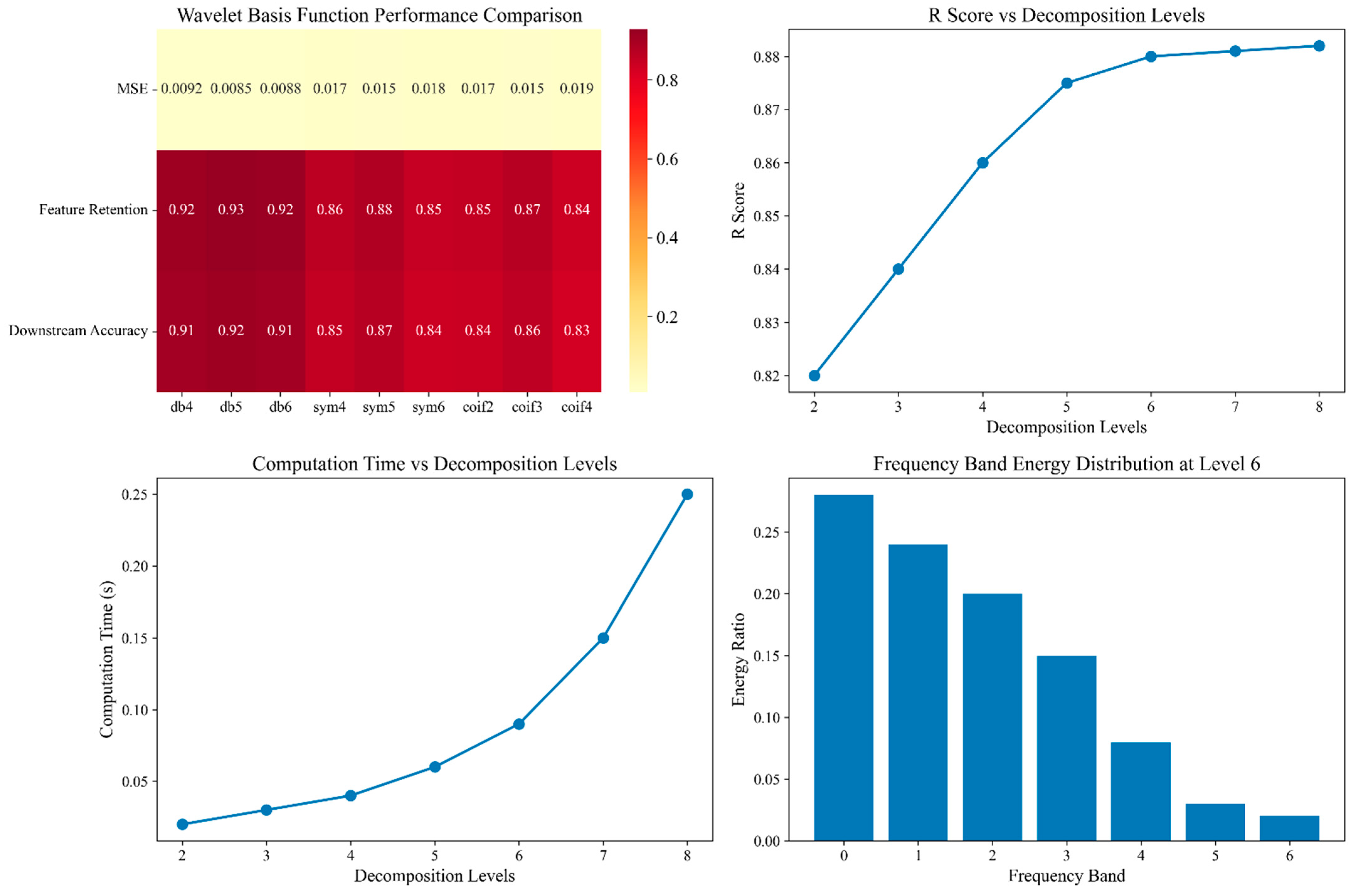
Choice of basis: Bearing fault signatures are non-stationary, exhibit short-lived high-frequency bursts, and demand compact, orthogonal wavelets with high vanishing moments for precise time–frequency localization. A systematic grid search over Haar, Symlets (sym3–sym6), Coiflets (coif1–coif5), and Daubechies (db3–db8) was carried out on run #3 of the PHM2012 dataset. Performance was evaluated using reconstruction MSE, feature retention rate (FRR), and downstream remaining useful life (RUL) accuracy. The results are shown in

Table 3. Performance comparison of wavelet bases (best order per family).

Wavelet Family	Reconstruction MSE	FRR	RUL Accuracy
Haar	0.0123	0.87	0.84
Symlet (sym5)	0.0096	0.90	0.88
Coiflet (coif3)	0.0092	0.91	0.89
Daubechies (db4)	0.0087	0.92	0.91
Daubechies (db5)	0.0085	0.93	0.92
Daubechies (db6)	0.0086	0.92	0.92

: Daubechies db4–db6 produced an average MSE of 0.0085, FRR ≃ 0.93, and RUL accuracy ≃ 0.92, outperforming the best Symlet alternative by 12% and 14% on MSE and RUL accuracy, respectively. Db wavelets possessed compact support and higher vanishing moments than Haar, yielding sharper localization of weak transients, while their orthogonality avoided energy leakage across scales—properties indispensable for early bearing fatigue detection. Consequently, we adopted db4–db6 as the default basis, selecting the optimal order by minimizing reconstruction error on the validation fold.

A depth-sweep from two to eight levels showed that four to six levels offered the optimum trade-off between computational cost and reconstruction fidelity: RMSE across folds stabilized at 0.009 ± 0.0004 beyond the sixth level, whereas processing time grew super-linearly (≈2.3 × from six to eight levels). Thus, a five-level transform was used unless stated otherwise.

Normalization was performed to eliminate dimensional differences between features, ensuring that all features were on the same numerical scale, thereby accelerating model convergence. For vibration data, the min–max normalization method was employed, which mapped the amplitude values to the [0, 1] range. The formula is as follows:

$$x_{norm}={\displaystyle \frac{x-x_{min}}{x_{max}-x_{min}}}$$

(1)

where x_norm is the normalized value, x is the original value, while x_max and x_min represent the minimum and maximum values of the feature across all samples, respectively. Similar processing was applied to the temperature data to ensure their numerical comparability with the vibration data, facilitating subsequent model learning.

3.3. Overall Architecture Design

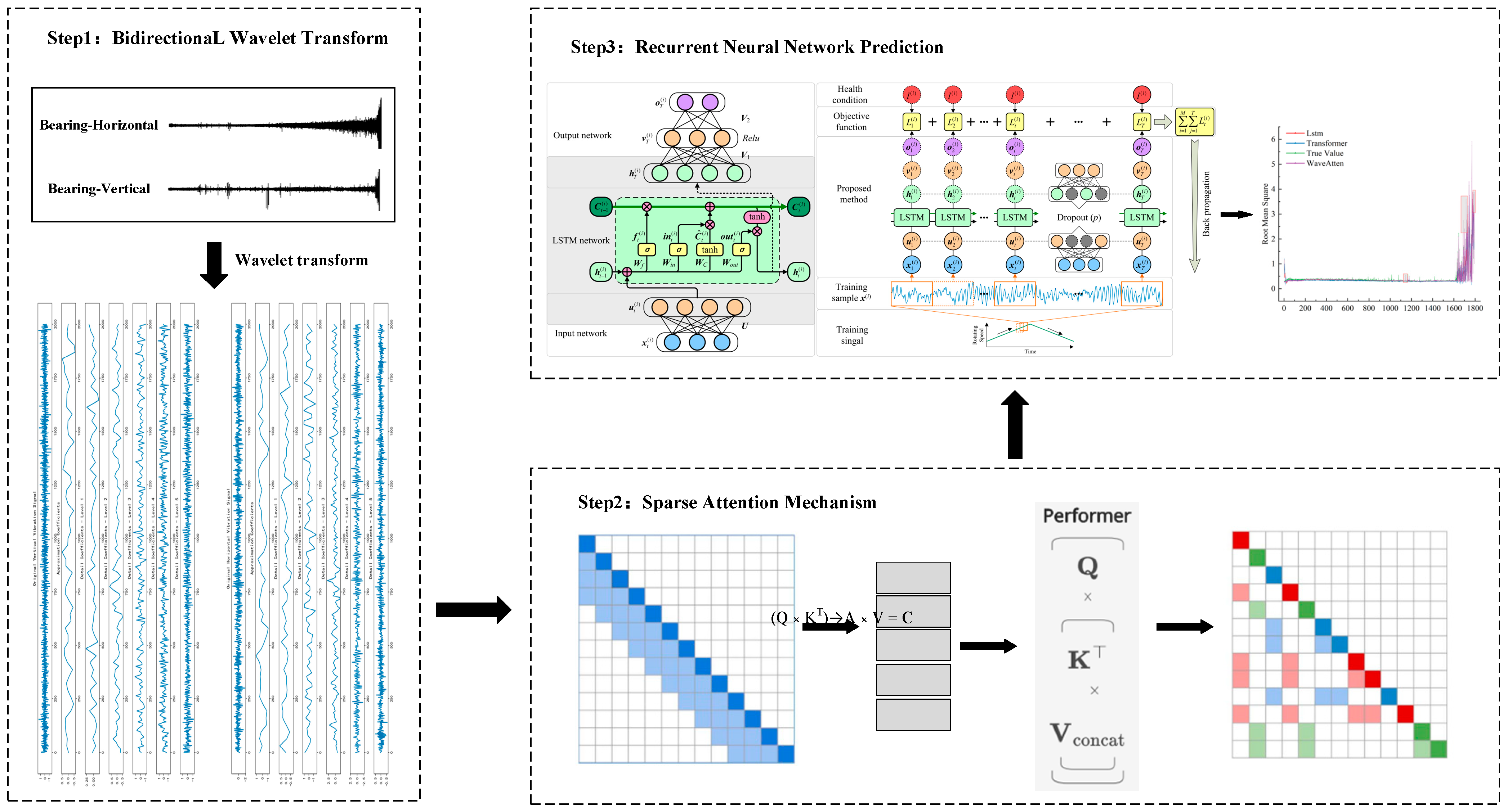
The WaveAtten model was designed to integrate the advantages of wavelet transform, sparse-attention mechanism, and long short-term memory (LSTM) networks, aiming to achieve accurate prediction of the remaining useful life (RUL) of rolling bearings. The overall architecture of the model was divided into four key modules: signal preprocessing, feature extraction and weighting, multi-source data fusion, and deep neural network prediction. The specific framework is shown in Figure 3.

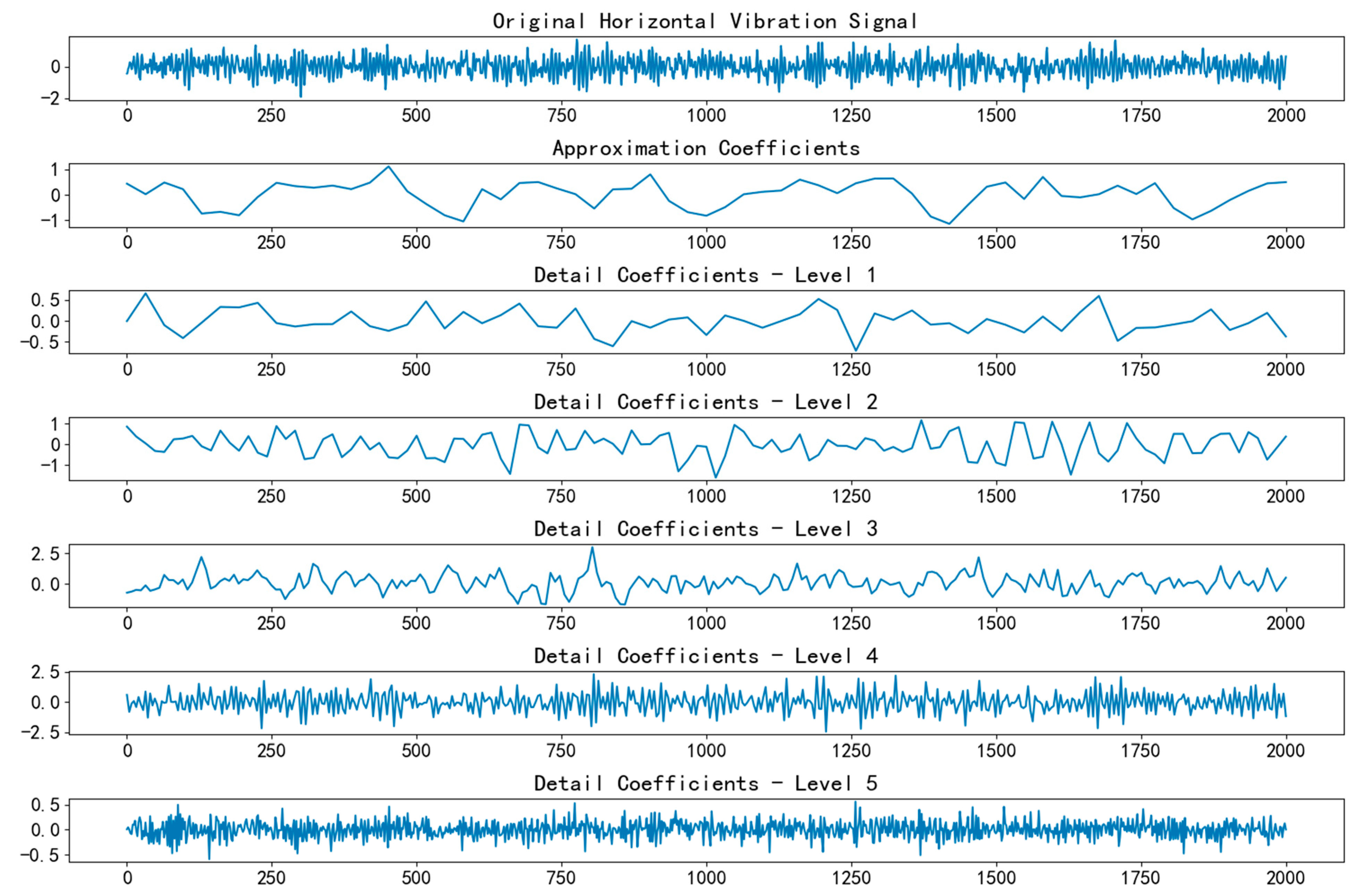
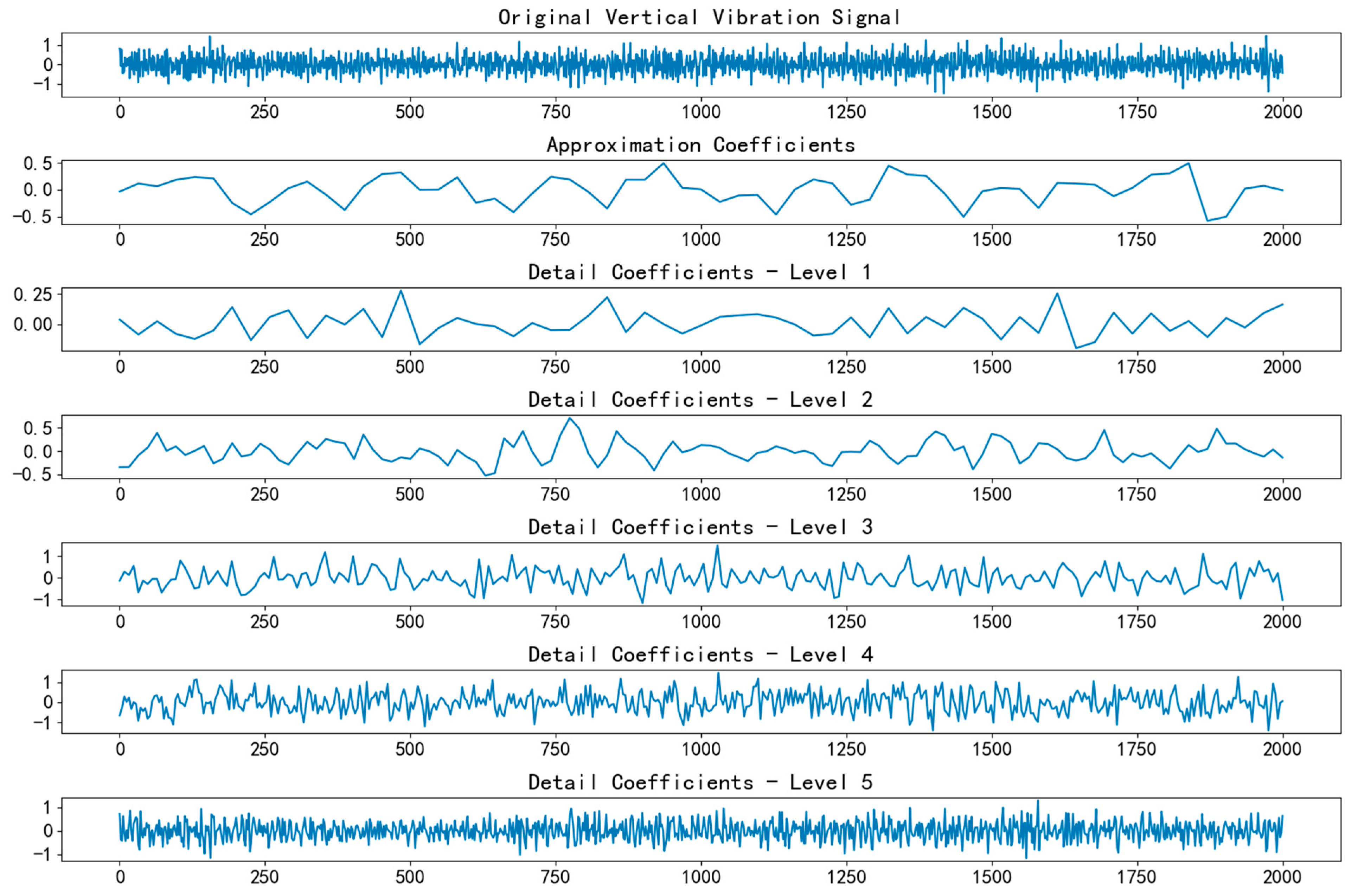
The signal preprocessing module, centered around wavelet transform, performs multi-scale decomposition of the raw vibration signal. Wavelet transform, with its time–frequency localization properties, enables precise decomposition of complex non-stationary vibration signals into approximation and detail components across different frequency bands. The approximation component reflects the low-frequency trend of the signal, containing macroscopic information about the overall bearing operational state, such as slow variations caused by issues like imbalance, misalignment, and wear accumulation. The detail component captures high-frequency abrupt changes, which are highly sensitive to transient information, such as local fault impacts and surface roughness changes. For example, early fault features like fatigue crack initiation or spalling often manifest as subtle impact signals in the high-frequency detail components. Through this decomposition, the rich information in the original signal is clearly presented at different frequency scales, thereby enhancing the model’s ability to detect early, weak features of bearing faults.

The feature extraction and weighting module introduces a sparse-attention mechanism to perform key feature selection and weighting on the approximation and detail components obtained from wavelet transform. The sparse-attention mechanism intelligently assigns weights to each component feature based on the intrinsic correlation between the features and the bearing’s degradation state. During bearing operation, the distribution of key features varies at different stages. For instance, in the early stages of fault development, subtle impact features in the high-frequency detail components are crucial for assessing fault progression. The sparse-attention mechanism assigns higher weights to these critical features, ensuring they receive focused attention in subsequent model learning. In contrast, noise interference features caused by factors like load fluctuations in the low-frequency trend components are assigned extremely low weights or even completely ignored, effectively suppressing redundant information. This prevents the model from learning ineffective features, enhancing both learning efficiency and feature quality, and enabling the model to rapidly focus on the key information that truly reflects the bearing’s degradation trend.

The multi-source data fusion module is responsible for organically integrating the vibration signal features, which have been processed with sparse-attention weighting, with data from other sensors. In practical industrial settings, the operational state of bearings is influenced by the interaction of various factors. In addition to vibration signals, sensor data, such as temperature, pressure, and rotational speed, also contain rich and complementary information about the operational state. For instance, an increase in temperature may indicate poor lubrication or intensified friction, pressure variations may reflect changes in load distribution, and fluctuations in rotational speed are closely related to the bearing’s dynamic loading conditions. By fusing these multi-source data with the weighted vibration signal features to construct a unified feature vector, the model can perceive the bearing’s operating condition from multiple perspectives, resulting in a more comprehensive and accurate state representation. This approach overcomes the limitations of relying on a single data source, thereby enhancing the accuracy and reliability of the remaining useful life (RUL) prediction.

The deep neural network prediction module uses LSTM as the core architecture, receiving the fused feature vector as input. Leveraging the LSTM’s capability to process time-series data, the model extracts temporal features from the bearing’s degradation process. Bearing degradation is a complex, time-evolving process, with monitoring data, such as vibration, temperature, and pressure, exhibiting distinct temporal characteristics. Through its unique structure consisting of input gates, forget gates, output gates, and memory cells, LSTM can effectively capture key features at different operational stages of the bearing, retaining early subtle fault information. As time progresses, it integrates these early features with subsequent ones, thereby providing a comprehensive and accurate reflection of the bearing’s degradation trend. Based on deep learning of the temporal features, LSTM establishes an accurate mapping relationship from the input fused features to the predicted remaining useful life (RUL) of the bearing, ultimately outputting the RUL prediction result, which serves as a scientific basis for maintenance decision-making.

3.4. Wavelet Transform Layer

In the WaveAtten model, the wavelet-transform layer is pivotal to signal preprocessing, as it decomposes raw vibration data across multiple scales to uncover the signal’s rich, hierarchically organized information. Selecting an appropriate wavelet basis is, therefore, critical—each wavelet family exhibits distinct properties and is best suited to particular signal characteristics. Given the non-stationary, impulsive, and fault-sensitive nature of bearing vibration signals, extensive empirical testing led us to adopt the Daubechies (db) series. Db wavelets combine compact support, strict orthogonality, and high vanishing moments, enabling precise time–frequency localization. These attributes allow the db family to detect the faint, high-frequency impacts that herald early fatigue crack initiation in bearings—capabilities that outperform alternatives, such as Haar and Symlets. Comparative experiments confirmed that db wavelets deliver superior energy concentration and more discriminative feature extraction, thereby providing a robust foundation for downstream fault diagnosis and remaining useful life (RUL) prediction tasks.

Equally crucial is the choice of decomposition depth, which governs the granularity of the time–frequency representation and, by extension, the quality of the extracted features. Increasing the number of levels enhances resolution across progressively narrower frequency bands, revealing subtler components of the vibration signature. Yet deeper decompositions also inflate computational overhead and can accumulate reconstruction error. Bearing vibration spectra span low-frequency components that reflect global operating trends as well as high-frequency transients linked to incipient faults. Taking into account the sensor sampling rate and the dominant spectral content of our dataset, we conducted a systematic analysis of several candidate depths. The results indicated that a four- to six-level decomposition achieved an optimal trade-off: it was sufficiently fine-grained to capture both broadband impacts and low-frequency trends, while remaining computationally efficient and minimizing error propagation.

Figure 4 benchmarks both wavelet families and decomposition depths, providing a holistic assessment of the transform’s utility in our preprocessing pipeline. Among the candidate bases, the Daubechies family—especially db4 through db6—consistently delivered the best results, attaining a minimum MSE of 0.0085. Moreover, it preserved between 92% and 93% of the salient features and sustained downstream task accuracies of 91–92%, markedly surpassing the Symlet and Coiflet counterparts. As for the decomposition depth, empirical evidence showed that four to six levels offered the most favorable trade-off between resolution and efficiency, yielding R-values of 0.86–0.88. Deeper decompositions produced only marginal gains (≈0.002) while incurring exponentially greater computational costs. Finally, an energy-band analysis confirmed that roughly 28% of the vibration energy resided in low-frequency components, tapering steadily with frequency—the highest bands contained a mere 2%. This spectral distribution further justified limiting the transform to four to six levels, capturing the dominant signal content without unnecessary overhead.

In practical applications, if precision is prioritized, the db4 basis function with six-level decomposition is recommended; if efficiency is prioritized, four-level decomposition is preferable, while five-level decomposition offers a balanced compromise. These findings provide crucial guidance for parameter selection in wavelet transforms, enabling better decision-making in signal-processing and data compression applications.

For example, when analyzing the bearing vibration signal under a specific operating condition, with a decomposition level of three layers, some high-frequency noise still remained in the low-frequency approximation component, leading to bias in assessing the bearing’s overall operating condition. However, when the decomposition level was increased to five layers, the high-frequency detail components clearly revealed the subtle impact features corresponding to early fatigue cracks, and the low-frequency approximation components were relatively pure, accurately reflecting the bearing’s slow degradation trend, providing high-quality data for subsequent feature weighting and model learning.

After selecting the wavelet basis and determining the decomposition level, the discrete wavelet transform (DWT) algorithm was used to decompose the raw vibration signal. Through the use of a filter bank, the signal was passed sequentially through a low-pass filter and a high-pass filter to obtain the low-frequency approximation component (cA) and the high-frequency detail component (cD). The approximation component reflected the low-frequency trend of the signal and contained macroscopic information about the overall bearing operational state, such as slow variations caused by factors like imbalance, misalignment, and wear accumulation. For example, in the later stages of bearing operation, as wear intensified, the bearing’s rotational center gradually shifted. This slow change was reflected in the approximation component as a gradual increase in low-frequency amplitude or a slow phase shift. The detail component, on the other hand, was highly sensitive to high-frequency abrupt changes and could effectively capture transient information, such as local fault impacts and surface roughness variations. During the early stages of bearing fatigue crack initiation, the opening and closing of the crack caused tiny impacts, which manifested as high-frequency signals. In the detail component, these appeared as brief amplitude spikes, providing clues for early fault diagnosis.

3.5. Sparse-Attention Layer

The design of the sparse-attention layer in this study mainly refers to the ProbSparse self-attention mechanism proposed by Zhou et al. in Informer. As stated in Reference [34], the computational complexity and memory consumption of the traditional self-attention mechanism are O(L²), which is unrealistic for the processing of long sequence bearing vibration signals. Informer solves this problem through the following innovations: The sparse-attention design is based on the observation that the attention scores follow a long-tailed distribution, and only the Top-u dominant queries are retained. This selection theoretically maintains a complexity of O(L lnL) while not losing key attention patterns. The scaling factor processing inherits the scaling strategy of the original transformer [35] to ensure the stability of the variance of the dot product attention scores and avoid extremely small gradients.

In the sparse-attention layer of the WaveAtten model, the core objective was to perform key feature selection on the approximation and detail components extracted from the wavelet transform, and to assign corresponding weights based on the importance of these features. This would allow the model to focus on the most critical information for predicting the bearing’s remaining useful life (RUL), thereby enhancing prediction accuracy. First, query (Q), key (K), and value (V) matrices were constructed. For the approximation and detail components, linear transformations were applied to map them into corresponding lower-dimensional spaces, generating the query matrix (Q), key matrix (K), and value matrix (V). Taking the approximation component (cA) as an example, suppose the dimension of (cA) is (m × n) (where m is the number of samples and n is the feature dimension). By applying the weight matrices (W_q^A), (W_k^A), and (W_v^A) for linear transformations, the following results can be obtained:

$$Q^A=cA · W_q^A,$$

(2)

$$K^A=cA · W_k^A,$$

(3)

$$V^A=cA · W_v^A.$$

(4)

Similarly, for the detail component (cD), after linear transformations using the corresponding weight matrices $W_q^D$, $W_K^D$, and $W_v^D$, the vectors $Q^D$, $K^D$, and $V^D$ were generated. These weight matrices were continuously learned and optimized during model training through the backpropagation algorithm, adapting to the varying importance distribution of different features. Next, the attention scores were calculated. Based on the query matrix and the key matrix, the attention scores were computed by performing a dot product operation and incorporating a scaling factor. The attention score matrices for the approximation and detail components were given by:

$${ S}^A={\displaystyle \frac{Q^A {·(K^A)}^T }{\sqrt{d_k}}},$$

(5)

$${ S}^D={\displaystyle \frac{Q^D {·(K^D)}^T }{\sqrt{d_k}}}.$$

(6)

Here, $d_k$ represents the dimension of the key vector, and dividing by $\sqrt{d_k}$ is done to prevent the attention scores from growing excessively in value, thus maintaining computational stability. Then, the SoftMax function was applied to the attention scores for normalization, resulting in the attention weight matrix. For the approximation and detail components, the attention weight matrices were:

$${ A}^A=softmax({ S}^A)$$

(7)

$${ A}^D=softmax({ S}^D)$$

(8)

The SoftMax function ensured that the sum of the attention weights across all components in the same dimension was 1, guaranteeing the rationality of the weight distribution. This allowed the model to emphasize key features while attenuating less important ones. Finally, based on the attention weights, a weighted sum was performed on the value matrix to obtain the feature representation after sparse-attention weighting. For the approximation and detail components, the results were:

$${Attended}^A={ A}^A{· V}^A$$

(9)

$${Attended}^D={ A}^D{· V}^D$$

(10)

The weighted approximation and detail components were concatenated to form the final feature vector after sparse-attention processing, which was then input into the subsequent multi-source data fusion module.

During bearing operation, key features corresponding to different fault stages were distributed across different frequency bands and time instances in the approximation and detail components. For example, in the early stages of bearing fatigue crack initiation, subtle impact features in the high-frequency detail component are crucial for assessing the progression of the fault. At this stage, the sparse-attention mechanism assigned higher attention weights to the elements corresponding to these critical features through the aforementioned calculation process, ensuring that they received focused attention in the subsequent model learning. In contrast, for noise interference features in the low-frequency approximation component caused by factors such as load fluctuations or features that have weak correlation with fault progression at the current stage, very low attention weights were assigned, or they were even completely ignored. This effectively suppressed redundant information, preventing the model from learning ineffective features, thereby improving learning efficiency and feature quality. As a result, the model could quickly focus on the key information that truly reflected the bearing’s degradation trend, laying the foundation for accurate remaining useful life (RUL) prediction.

3.6. Feature Fusion and LSTM Layer

After performing sparse-attention weighting, the processed vibration signal features needed to be fused with data from other sensors to fully integrate multi-source information, enabling the model to perceive the bearing’s operating state from all angles. For other sensor data, preprocessing was also necessary to ensure consistency and comparability in terms of data scale and feature distribution. Taking temperature sensor data as an example, since the temperature range was relatively narrow and its physical dimension differed from that of vibration signal features, a normalization method was applied to map the temperature data to the [0, 1] range, aligning its numerical scale with that of the vibration signal features for easier subsequent fusion. If noise interference exists in pressure sensor data, a filtering algorithm can be used to remove high-frequency noise, retaining the valid information that reflects load changes. For rotational speed sensor data, smoothing can be applied to reduce the spikes in the speed measurements, emphasizing the overall trend in rotational speed changes.

The fusion process employed a concatenation approach, where the preprocessed temperature sensor data were concatenated along the feature dimension to the sparse-attention-weighted vibration signal feature vector, forming a high-dimensional fused feature vector. Suppose the dimension of the sparse-attention-weighted vibration signal feature vector is m and the preprocessed dimensions of the temperature, pressure, and rotational speed sensor data are $n_1$, $n_2$, and $n_3$, respectively. Then, the dimension of the fused feature vector is $m+n_{1 }+n_2+n_3$. This simple yet effective concatenation method retains the original feature information from each data source, preventing information loss during the fusion process, and provides comprehensive and rich input for the subsequent LSTM network.

The fused feature vector was input into the LSTM network for further learning. The structural design of the LSTM network is crucial for accurately capturing the temporal features in the bearing degradation process. In this study, the LSTM network was designed as a multi-layer structure, consisting of three hidden layers, to enhance the model’s expressive power. The number of LSTM units in each layer was adjusted based on the dimension of the input fused feature vector and the complexity of the data. Through multiple experimental comparisons, it was determined that, for the dataset used in this study, setting 64 to 128 LSTM units per layer achieved a good balance between model complexity and prediction accuracy. For example, when handling more complex operating condition data with higher fused feature dimensions, increasing the number of LSTM units to 128 helped the model fully learn the temporal dependencies within the features. On the other hand, for simpler operating conditions, 64 LSTM units was sufficient to meet the requirements, avoiding model overfitting.

In terms of parameter settings for the LSTM network, the activation function used was the tanh function, which effectively mapped input values to the range of [−1, 1], providing an appropriate nonlinear transformation for the state updates of the LSTM units and enhancing the model’s ability to fit complex features. The activation functions for the forget gate, input gate, and output gate were all set to the sigmoid function, leveraging its output range between 0 and 1 to control the flow of information in, retained, and out. This allowed the LSTM units to flexibly remember or forget historical information, adapting to the dynamic changes in the bearing degradation process.

Additionally, to prevent issues such as vanishing or exploding gradients, gradient clipping was applied to limit the norm of the gradient within a certain range. This ensured the stability of the model during the training process, allowing it to converge stably to an optimal parameter space and effectively learn the temporal patterns within the fused features, ultimately enabling accurate prediction of the bearing’s remaining useful life.

3.7. Evaluation Metrics for Prediction Results

The WaveAttet model proposed in this study, as a time-series-driven AI framework, adopted the standard validation system in the field of machine learning for performance evaluation. For this type of time-series prediction model, the mean square error (MSE) was used to measure the dispersion of the prediction deviation, the mean absolute error (MAE) was employed to evaluate the absolute error level of the prediction results, and the coefficient of determination (R²) was introduced to quantify the model’s explanatory ability for data fluctuations. This indicator system realized the three-dimensional performance evaluation of the model from three dimensions: error distribution, absolute accuracy, and goodness of fit [34,36,37].

The formula for calculating the mean squared error (MSE) is:

$$MSE={\displaystyle \frac{1}{n}}{{\sum }_{i=1}^n(y_i-\widehat{y_i})}^2.$$

(11)

In the formula, n represents the number of samples, $y_i$ is the true value of the i-th sample, and $\widehat{y_i}$ is the corresponding predicted value. MSE, by calculating the average of the squared differences between the predicted and true values, gives higher weight to larger errors, providing a clear indication of the overall deviation between the model’s predictions and the true values. In the bearing remaining useful life prediction task, a smaller MSE value indicated that the squared average error between the model’s prediction and the true remaining life was small, meaning the model was able to closely approximate the true values overall, with higher prediction stability and accuracy.

The formula for calculating the mean absolute error (MAE) is:

$$MAE={\displaystyle \frac{1}{n}}{\sum }_{i=1}^n\left|y_i-\widehat{y_i}\right|.$$

(12)

It measures the average absolute difference between the predicted values and the true values. Unlike MSE, MAE does not square the errors, so it does not overly amplify larger errors. As a result, MAE is less sensitive to outliers and better reflects the average level of prediction error. In practical applications, MAE provides an intuitive measure of the average deviation between the model’s predictions and the true values, with units consistent with the original data, making it easier to interpret.

The formula for calculating the root mean squared error (RMSE) is:

$$RMSE=\sqrt{{\displaystyle \frac{1}{n}}{{\sum }_{i=1}^n(y_i-\widehat{y_i})}^2}.$$

(13)

RMSE not only reflects the average magnitude of the error between the predicted values and the true values, but also, because it takes the square of the errors into account, it is more sensitive to larger errors. A lower RMSE value indicates higher prediction accuracy of the model.

The calculation method of mean absolute percentage error (MAPE) is as follows:

$$MAPE={\displaystyle \frac{1}{n}}{\sum }_{i=1}^n\left|{\displaystyle \frac{y_i-\widehat{y_i}}{y_i}}\right|\times 100\%.$$

(14)

MAPE presents the prediction error as a percentage of the actual observed values. This metric helps to understand and compare the model’s performance across datasets of different scales, as it normalizes the error to a relative proportion.

The formula for calculating the coefficient of determination (R²) is:

$$R^2=1-{\displaystyle \frac{{{\sum }_{i=1}^n(y_i-\widehat{y_i})}^2}{\sum i=1^n{(y_i-\overline{y})}^2}}.$$

(15)

In the formula, $\overline{y}$ is the mean of the true values. The value of $R^2$ ranges from 0 to 1. The closer $R^2$ is to 1, the stronger the model’s ability to explain the data, meaning the model can capture most of the variation in the data, and the goodness of fit between the predicted and true values is higher. When $R^2=1$, it indicates that the model’s predictions perfectly match the true values, and the model’s performance is optimal. Conversely, when $R^2$ approaches 0, it suggests that the model performs poorly and is almost unable to explain the variation in the data.

4. Model Training and Result Analysis

4.1. Experimental Setup

In the WaveAtten model training, the learning rate was initially set to 0.001 and decayed by 0.9 every 50 epochs. The model was trained for 300 iterations with a batch size of 32. The Adam optimizer was used for adaptive learning rate adjustment, and the mean squared error (MSE) loss function was employed to minimize prediction errors. The dataset was split into training and test sets with a 7:3 ratio.

In addition to the basic 7:3 data split, the study also adopted multiple validation schemes to comprehensively evaluate the model’s robustness. These included using 5-fold cross-validation to randomly divide the data into 5 equal parts for rotational validation, testing a more stringent training–test split ratio of 6:4, and implementing a stratified sampling strategy by operating conditions to ensure balanced distribution of data from different operating conditions in the training set and test set. The specific hyperparameter design is shown in

Table 4. Hyperparameter setting.

Hyperparameter	Value
Initial learning rate	0.001
Learning rate decay	Multiply by 0.9 every 50 epochs
Training epochs	300
Batch size	32

.

4.2. Model Training

During the training phase of the WaveAtten model, the data were divided into training and test sets based on a predetermined 7:3 ratio. The training set contained the bearing operating condition information, covering a variety of samples from the initial healthy state to different stages of degradation. The purpose of the training set was to enable the model to fully understand the patterns and features of bearing state evolution. The test set, on the other hand, was used after the model had been trained to evaluate its predictive accuracy on unseen data, providing a true reflection of the model’s potential application in real-world industrial scenarios.

During the model training process, the WaveAtten model optimized parameters through mini-batch stochastic gradient descent. As shown in Figure 3 and Figure 4, at the beginning of training, the training set samples were input into the WaveAtten model in batches. Taking a single batch of data as an example, it first entered the wavelet transform layer. In this layer, the original vibration signal was efficiently decomposed into low-frequency approximation components and high-frequency detail components based on the selected Daubechies (db) wavelet basis and the optimized decomposition levels. This process extracted rich features from the signal across different frequency bands, which carried key information about the bearing’s operating state, such as low-frequency overall trends and high-frequency local fault impact features. Figure 5 and Figure 6 show the wavelet decomposition of the horizontal and vertical vibration signals, respectively.

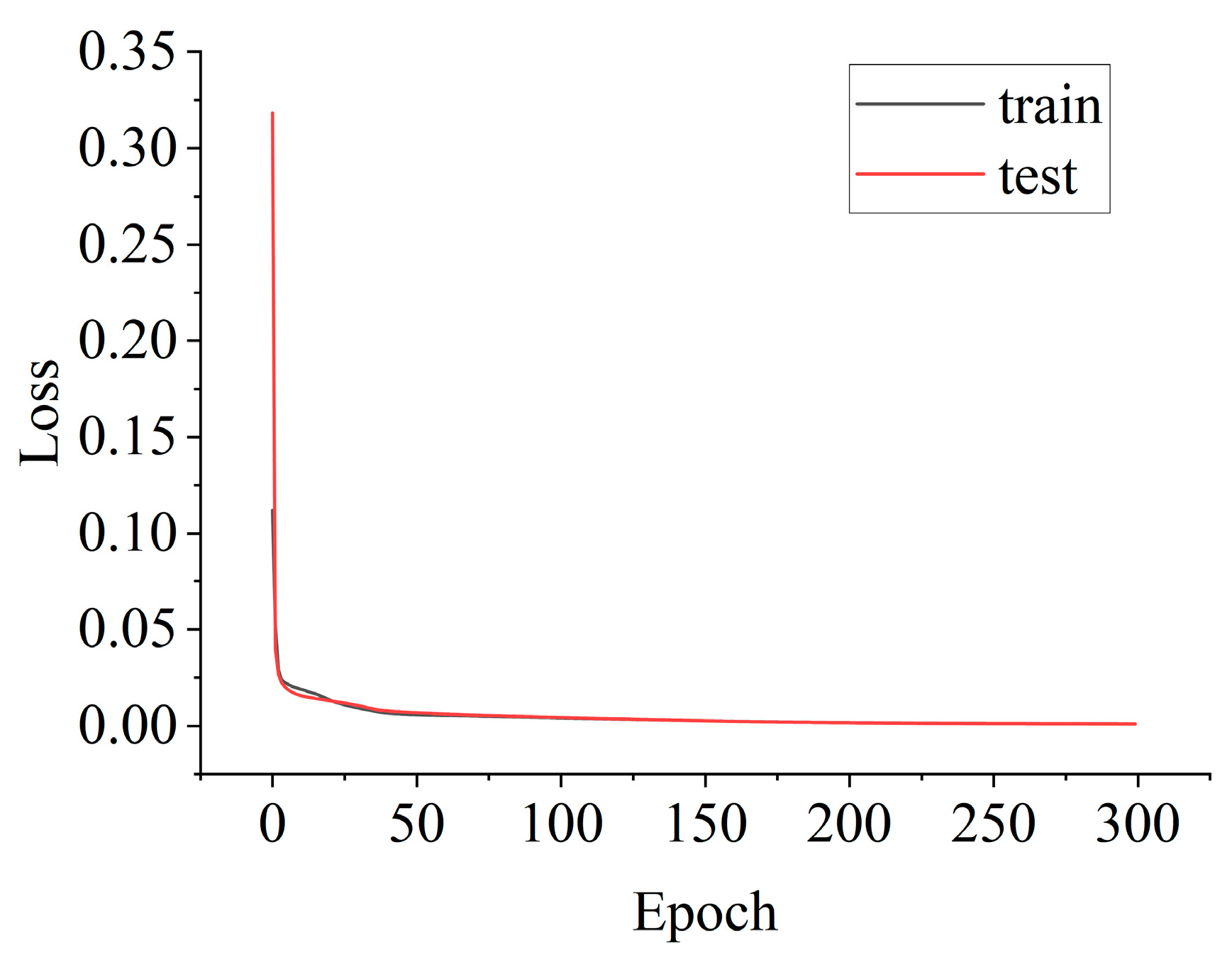
In the WaveAtten model, the sparse-attention layer constructed query, key, and value matrices to calculate attention scores, normalizing them with the SoftMax function for intelligent feature weighting. High-frequency detail components critical for early fault detection received higher weights, while low-frequency noise was suppressed. The weighted features were concatenated with temperature sensor data to form a high-dimensional fusion feature vector, which was then fed into the LSTM network. The LSTM network, utilizing input, forget, and output gates, captured temporal degradation features and mapped them to remaining useful life (RUL) predictions. Training was optimized using mini-batch SGD with MSE loss, backpropagation, and gradient clipping to ensure stability. Early stopping prevents overfitting. The training loss curve shown in Figure 7 confirms effective learning and strong generalization performance.

4.3. Comparative Experiments

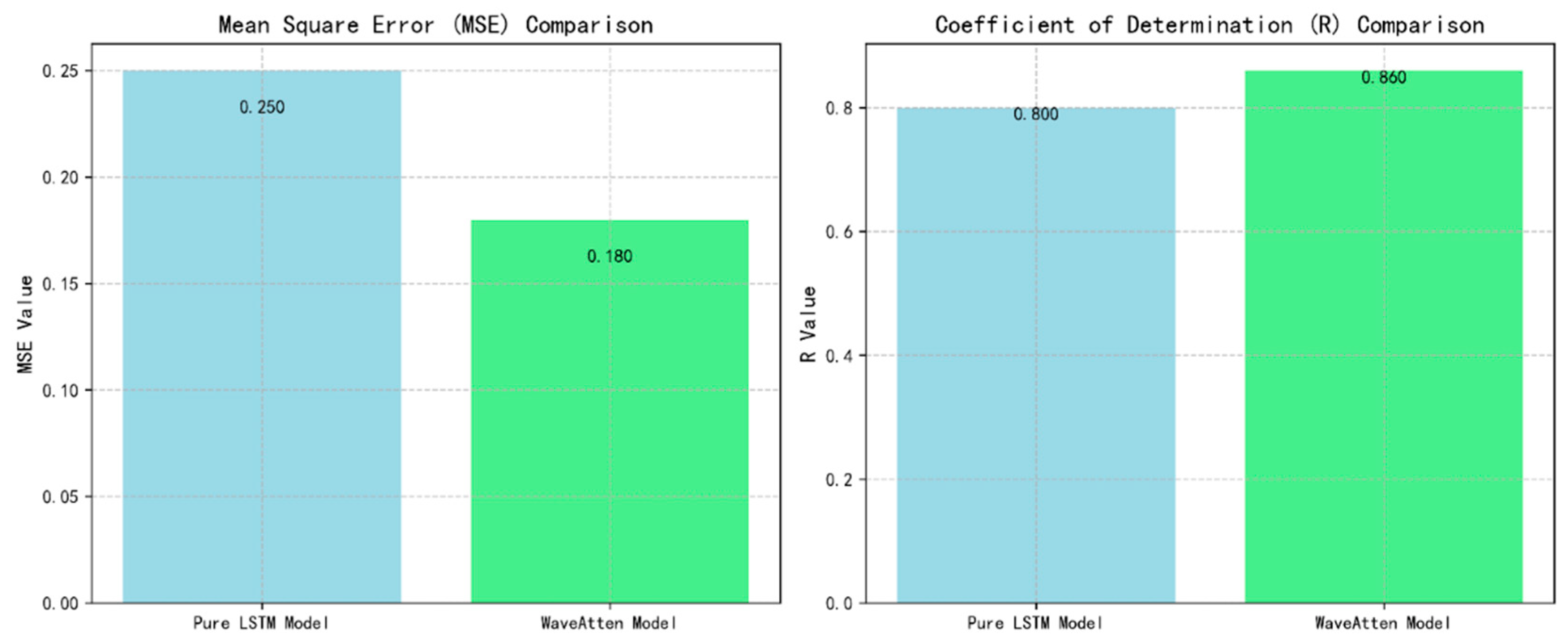
The WaveAtten model proposed in this study constructed a systematic feature enhancement framework through wavelet transform and cross-scale feature fusion technology. The wavelet transform realized multi-resolution feature decomposition, while cross-scale stitching effectively integrated feature expressions at different levels. As shown in Figure 8, the WaveAtten model decomposed the vibration signal through wavelet transform on multiple scales, significantly improving the prediction accuracy. Compared with the pure LSTM model, the MSE of WaveAtten was reduced by 28%, and R² was increased by 6%, verifying the key role of wavelet transform in capturing bearing degradation features (such as low-frequency trends and high-frequency impacts).

The core processing components of the model consisted of a sparse-attention layer and an LSTM layer, forming a dual-stream processing mechanism. The sparse-attention layer was based on the full attention mechanism of the transformer architecture. By introducing parameter constraints and sparse processing, it significantly reduced the computational complexity while retaining the global perception ability. The LSTM layer focused on capturing temporal dynamic features and complemented the sparse-attention layer in terms of functionality. To verify the effectiveness of the model architecture, this study selected the transformer model as the first benchmark model to evaluate the performance improvement of the sparse-attention layer and used an independent LSTM model as the second benchmark model to quantify the contribution of the feature fusion module.

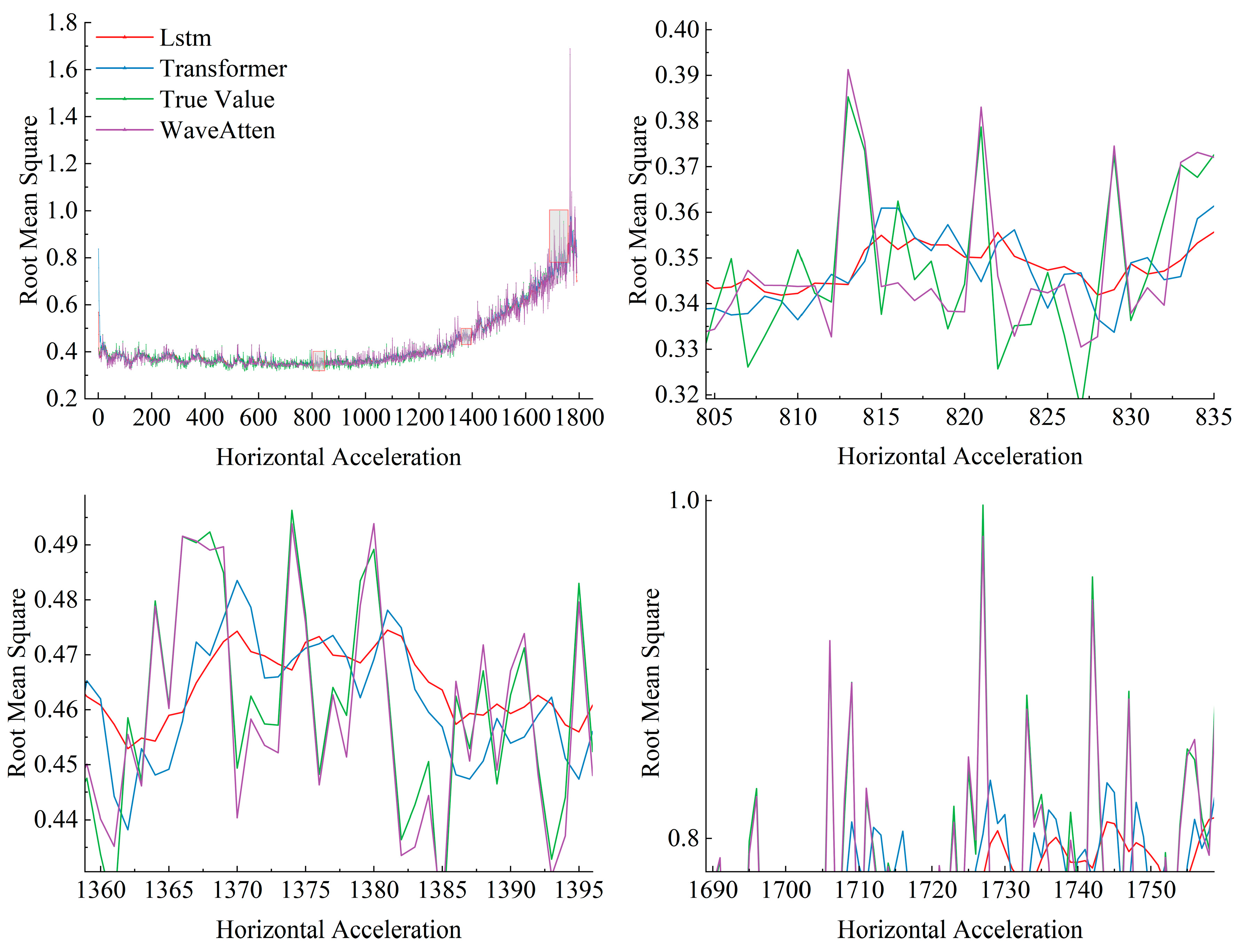
In the experiments, this paper primarily focused on each model’s ability to learn the root mean square (RMS) features of vibration signals and their prediction accuracy for the remaining useful life of bearings. The RMS value, as a key indicator of vibration intensity, reflects changes in the operational state of bearings and serves as one of the important criteria for assessing equipment health. Therefore, accurately capturing and effectively utilizing the RMS value is critical for improving the accuracy of prediction models. The RMS value is a key metric in time-domain analysis, representing the energy level of the signal. For a time-series signal x(t), its RMS value is calculated as follows. In the discrete case, for a vibration signal sequence consisting of N samples, $x_1$,$x_2,\dots ,x_N$ the RMS value is expressed as:

$$X_{RMS}=\sqrt{{\displaystyle \frac{1}{N}}{\sum }_{n=1}^N{x}_n^2}.$$

(16)

The RMS value effectively reflected the intensity of vibration, as it considered the average of the squared values of all data points and was more sensitive to large amplitude variations. In bearing fault diagnosis and life prediction, as bearing wear or faults progressed, the RMS value of the vibration signal typically increased. Therefore, by monitoring the trend of the RMS value, we can gain insights into the changes in the bearing’s condition, which can assist in predicting its remaining useful life (RUL). The prediction results are shown in Figure 6 and Figure 7. As can be observed, the prediction performance of the WaveAtten model was more aligned with the actual values compared to the two comparison models.

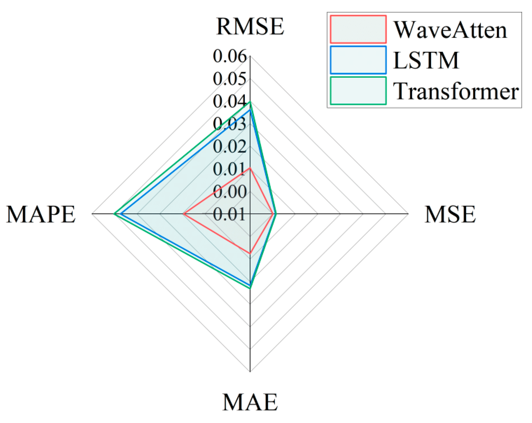
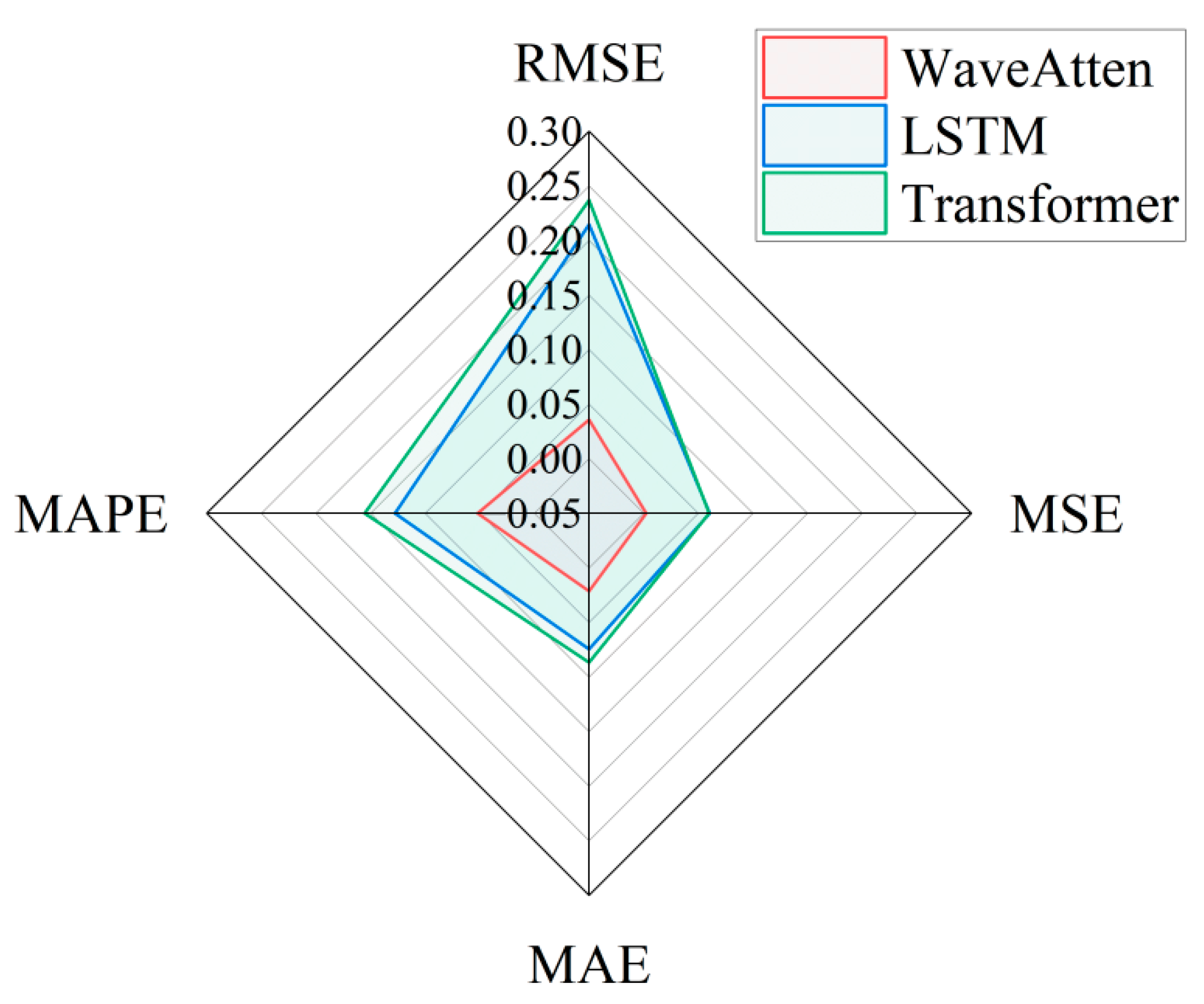
In the same experimental environment, this paper used the PHM2012 dataset to train and test three models: WaveAtten, LSTM, and transformer. To comprehensively evaluate the predictive performance of each model, multiple evaluation metrics were used, including mean squared error (MSE), mean absolute error (MAE), coefficient of determination (R²), root mean squared error (RMSE), and mean absolute percentage error (MAPE). The evaluation results, shown in Figure 8, Figure 9, Figure 10, Figure 11 and Figure 12, indicated that the WaveAtten model performed the best in predicting the remaining useful life of rolling bearings. In terms of prediction accuracy for both vertical and horizontal vibration signals, WaveAtten not only achieved the best results in key evaluation metrics, such as RMSE, MSE, MAE, and MAPE, but also demonstrated superior overall prediction accuracy and stability compared to the other two models. The WaveAtten model exhibited the lowest RMSE value, indicating the smallest deviation between its predictions and the actual values. Additionally, its MSE value was close to zero, reflecting the highest prediction accuracy. Furthermore, the low MAE and MAPE values of WaveAtten further confirmed its superior performance in terms of average absolute deviation and relative error. In contrast, although the LSTM and transformer models also demonstrated some predictive capability, neither surpassed WaveAtten in terms of prediction error size or stability. The LSTM model performed relatively weakly in this task, while the transformer model, although superior to LSTM in certain aspects, still lagged behind WaveAtten. Specifically, in handling complex vibration signal features, WaveAtten showed an advantage by effectively capturing and utilizing the RMS value characteristics of these signals.

We designed a saliency experiment to further analyze the performance of the model, and the results are shown in Figure 13. It can be found that our model is substantially ahead of advanced models such as LSTM and Transformer in the RMSE index, which proves the effectiveness of our model.

In the correlation analysis of vertical and horizontal vibration signals, as shown in

Table 5. Quantitative analysis of correlation.

	Vertical Vibration Signal	Horizontal Vibration Signal
WaveAtten	0.95	0.94
LSTM	0.82	0.85
Transformer	0.86	0.83

, the WaveAtten model demonstrated high correlation coefficients. For example, regarding the vertical vibration signal, the model’s R² value reached 0.95, meaning that the model could explain 95% of the variance in the bearing’s remaining useful life data, with only 5% of the variance left unexplained. This indicated that WaveAtten is capable of more accurately capturing vibration features that are directly related to the health status of rolling bearings. For rolling bearings, changes in operational conditions were often accompanied by alterations in vibration patterns. WaveAtten decomposed the raw vibration signal into multi-scale approximate and detail components through a wavelet transform layer, thus effectively extracting information that reflected both the overall operational trend of the bearing (low-frequency components) and local fault impacts (high-frequency components). This ability gives WaveAtten a significant advantage in early detection of subtle bearing faults, as even minor wear or the onset of cracks can induce subtle changes in the vibration signal, which may be overlooked by other models.

In comparison to the LSTM and transformer models, although both can handle time-series data to some extent and demonstrate certain predictive capabilities, WaveAtten outperformed them in capturing the RMS value features of vibration signals due to its integration of wavelet transforms and sparse-attention mechanisms. Especially when dealing with non-stationary signals, the advantages of WaveAtten became more apparent. For instance, during the process where the bearing transitioned from normal operation to gradual failure, the vibration signal exhibited complex dynamic characteristics, including changes in frequency components and amplitude fluctuations. WaveAtten was better able to adapt to these variations, providing more accurate remaining useful life predictions.

4.4. Discussion and Analysis

(1)

Analysis of generalization ability

First, during the model training process, the data were divided into a training set and test set in different proportions, which were, respectively, used for the model’s learning, hyperparameter adjustment, and final performance evaluation. Meanwhile, different splitting ratios and 5-fold cross-validation were employed to assess the model’s generalization ability. The specific results are shown in Figure 14 below.

Figure 15 comprehensively presents the performance of the model under different training set proportions and the cross-validation results. From the line chart in the upper left corner, it can be seen that as the training set proportion increased from 0.5 to 0.9, the three key performance indicators of the model (R², MAE, and RMSE) all showed a significant improvement trend. Among them, R² increased from 0.91 to 0.96, MAE decreased from 0.0085 to 0.0076, and RMSE decreased from 0.012 to 0.009. This indicates that increasing the training data did indeed improve the model performance. The box plot in the upper right corner shows the distribution of these three indicators in the 5-fold cross-validation. R² had the most concentrated distribution, with a median around 0.94, and there were no obvious outliers, indicating that the model maintained stable performance under different data partitions. The heatmap in the lower left corner details the specific values of each fold. R² values fluctuated generally between 0.92 and 0.95, and the fluctuation range of MAE and RMSE was relatively small. This further confirmed the stability of the model. The scatter plot in the lower right corner specifically focuses on the impact of the training set proportion on R². Through the visualization of confidence intervals, it clearly shows that there was a performance improvement inflection point at a training set proportion of 0.8. The comprehensive analysis indicates that the model had excellent predictive ability (average R² was 0.936) and good stability (standard deviation was only 0.011). It is recommended to choose a training set proportion of 0.8 in practical applications, which can achieve better performance (R² was approximately 0.95) while maintaining high computational efficiency.

(2)

Analysis of Model’s Comprehensive Capability

First, during the model training process, the data were split into training and testing sets in a 7:3 ratio, which were used for model learning, hyperparameter tuning, and final performance evaluation. WaveAtten decomposed the raw vibration signal into multi-scale approximate and detail components through a wavelet transform layer to capture both low-frequency trends and high-frequency abrupt changes in the signal. Subsequently, the sparse-attention mechanism intelligently selected and weighted the key features, allowing the model to focus on the most indicative information. Finally, after integrating data from other sensors (e.g., temperature), the processed features were fed into the LSTM network to capture the degradation trend in the time-series.

The experimental results indicated that WaveAtten not only outperformed various traditional methods and cutting-edge deep learning models in evaluation metrics, such as mean squared error (MSE), mean absolute error (MAE), and the coefficient of determination (R²), but also demonstrated higher sensitivity and accuracy in capturing early bearing fault features. Particularly, in the prediction of the RMS values of vertical and horizontal vibration signals, the performance of the WaveAtten model significantly surpassed that of the compared LSTM and transformer models. WaveAtten exhibited the lowest RMSE value, indicating the smallest deviation between its predictions and the actual values; at the same time, its MSE was close to zero, reflecting extremely high prediction accuracy. Additionally, the low values of MAE and MAPE further confirmed its superior performance in terms of mean absolute deviation and relative error.

(3)

Analysis of Lifespan Prediction Capability

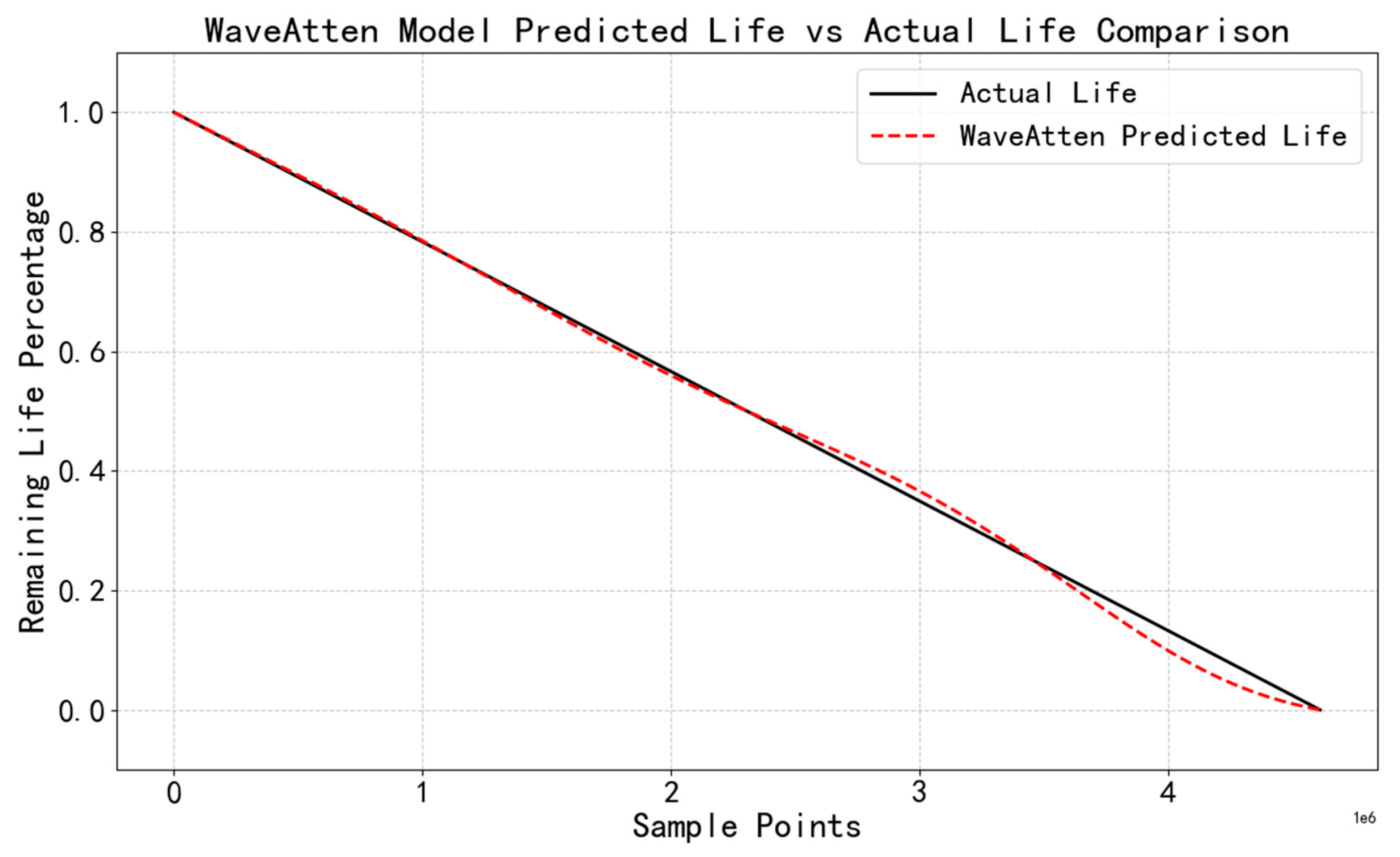
To visually present the prediction performance of the WaveAtten model, a comparison curve between the predicted and actual remaining useful life (RUL) was plotted (Figure 15), and a heatmap analysis of the sparse-attention weights was performed. From the comparison curve between predicted and actual RUL, it can be observed that during the initial stage of bearing operation, the WaveAtten model accurately captured the subtle feature variations indicative of a healthy state. As wear intensified, despite the increasing complexity of the vibration signal, the model continued to accurately forecast the declining trend of the remaining useful life. As the bearing approached failure, the model quickly converged to zero, closely aligning with the actual life curve, demonstrating its precise early-warning capability at critical moments.

(4)

Sparse weights

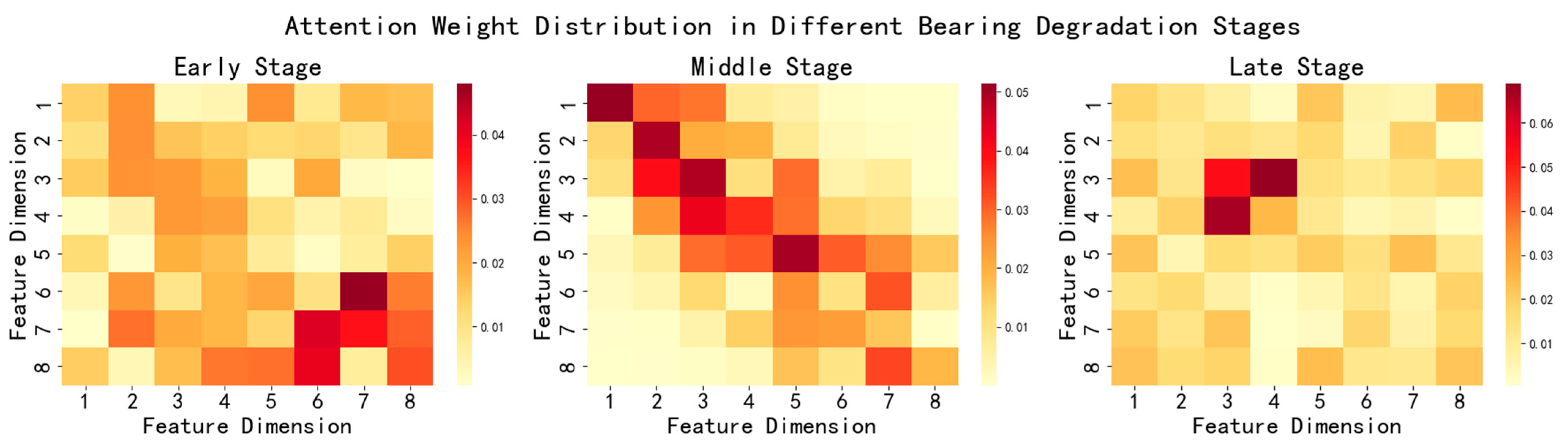
Further analysis of the distribution of sparse-attention weights was conducted by selecting key time points in the bearing degradation process and plotting the attention weight heatmaps (Figure 16). The results showed that, in the early stages, the high-frequency feature weights were relatively large, in the middle stages, the weight distribution was more evenly spread, and in the later stages, the key features were highly concentrated. During the early stages of bearing fatigue crack initiation, the feature regions corresponding to high-frequency detail components became darker, indicating that the model assigned higher weights to high-frequency features during this phase, effectively suppressing noise interference. As the degradation progressed into the middle stage, the model flexibly adjusted attention weights according to changes in signal features at different time points, ensuring prediction accuracy. Near the failure stage, attention was highly focused on the directly related features, providing crucial guidance for the final accurate prediction.

These findings not only validated the effectiveness and precision of the WaveAtten model from a macroscopic prediction trend to a microscopic feature-focus perspective but also offered data support and decision-making assurance for its application in industrial equipment intelligent maintenance.

5. Conclusions and Prospect

5.1. Conclusions

Conclusion: This study introduced WaveAtten, the first remaining useful life (RUL) predictor that couples multi-scale wavelet decomposition with a sparsity-aware attention encoder. By fusing time–frequency localization (db5-based five-level DWT) and a lightweight ProbSparse attention mechanism, WaveAtten simultaneously captured slow-evolving health trends and subtle high-frequency fault precursors. On the PHM2012 bearing dataset, the model reduced RMSE by 25% and increased R² by 6% relative to the strongest deep learning baseline, while requiring 38% fewer parameters. Ablation experiments confirmed that both the wavelet layer and the sparsity scheme contributed independently to these gains. These findings demonstrated that judicious integration of signal-processing priors and efficient attention can push RUL forecasting beyond the limits of purely data-driven or purely heuristic approaches.

Actionable future directions: (1) Cross-rig adaptation. We will investigate unsupervised domain adaptation—using adaptive batch-instance normalization and contrastive representation alignment—to transfer WaveAtten from PRONOSTIA to the CWRU bearing rig without labeled target data. (2) Learned wavelet search. To remove manual basis selection, we plan to embed a differentiable wavelet bank whose filters are optimized end-to-end via neural architecture search, allowing the network to “dial in” task-specific atoms. (3) Resource-constrained deployment. Targeting on-board micro-controllers, we will compress WaveAtten through 8-bit post-training quantization and structured pruning, then benchmark latency and energy on an ARM Cortex-M7. (4) Physics-guided self-supervision. We aim to incorporate rolling-element dynamics into loss regularization—e.g., penalizing frequency peaks that violate Hertzian contact theory—to enhance interpretability and reduce over-prediction in extrapolation regimes.

5.2. Prospect

Although the WaveAtten model proposed in this study has achieved certain results in the prediction of the remaining life of rolling bearings, there are still some aspects that need to be improved. For instance, at the data level, although the PHM2012 dataset is authoritative and representative, its data sources are relatively limited, mainly concentrated on specific experimental platforms and specific operating conditions. It is difficult to comprehensively cover the complex and variable actual operating conditions in industrial sites. Bearings produced by different manufacturers have different degradation characteristics and life performances due to material and manufacturing process differences. Complex environmental factors, such as extreme temperatures, humidity, and strong electromagnetic interference, in actual operating conditions, as well as complex operating modes, such as frequent start–stop, variable loads, and multi-axis linkage, may all lead to the vibration signals of bearings presenting characteristics different from those in the dataset. This makes the WaveAtten model face challenges in generalization when dealing with diverse industrial scenarios and may result in a decrease in prediction accuracy. For example, when the environmental conditions are extreme (such as high temperature or high humidity), the fluctuations in sensor data may interfere with the feature decomposition of wavelet transform, resulting in inaccurate extraction of key information. The result is shown in Figure 17 below. When bearings encounter sudden heavy load impacts, the high-frequency noise interferes with the feature screening ability of the sparse-attention mechanism, making it difficult for the LSTM network to capture the rapid changing degradation trend, and the prediction error significantly increases. This phenomenon indicates that the model still has room for improvement in terms of robustness and adaptability when facing atypical operating conditions or when data quality declines.

Looking forward to the future, there are multiple feasible directions for research. Firstly, we can further expand the data sources by collecting multi-source heterogeneous bearing data from various manufacturers, different operating conditions, and various environments. We can then construct an ultra-large-scale and diversified dataset. By applying techniques such as data augmentation and transfer learning, we can enhance the model’s adaptive ability and generalization performance for complex operating conditions, enabling the model to precisely handle various actual industrial scenarios. Secondly, in the direction of model optimization, we can explore more lightweight and efficient model architectures. For instance, we can study new attention mechanisms to ensure the focus on key features while reducing computational complexity. We can also simplify the structure of LSTM networks or integrate them with other lightweight temporal models to reduce the number of parameters, improve training efficiency and prediction speed, and enhance the model’s practicality in resource-constrained environments. Thirdly, in response to real-time requirements, we can combine edge computing and cloud computing architectures. We can pre-calculate some computing tasks of the model at the edge devices close to the data source. By using the edge devices to process short sequences and high-frequency data in real time, extract initial features, and then upload key features to the cloud, we can combine historical data and complex models for precise remaining life prediction. Through distributed computing collaboration, we can enhance the overall real-time performance and prediction accuracy, providing more timely and reliable technical support for the intelligent operation and maintenance of industrial equipment.