Structured Stability of Hybrid Stochastic Differential Equations with Superlinear Coefficients and Infinite Memory

Abstract

The stability of hybrid stochastic differential equations (SDEs in short) depends on multiple factors, such as the structures and parameters of subsystems, switching rules, delay, etc. Regarding stability analysis for hybrid stochastic systems incorporating subsystems with diverse structures, existing research results require the system to possess either Markovian properties or finite memory characteristics. However, the stability problem remains unresolved for hybrid stochastic differential equations with infinite memory (hybrid IMSDEs in short), as no systematic theoretical framework currently exists for such systems. To bridge this gap, this paper develops a rigorous stability analysis for a class of hybrid IMSDEs by introducing a suitably chosen phase space and leveraging the theory of fading memory spaces. We establish sufficient conditions for exponential stability, extending the existing results to systems with unbounded memory effects. Finally, a numerical example is provided to illustrate the effectiveness of the proposed criteria.

1. Introduction

Delay (memory) and uncertainty cannot be ignored in system modeling. As a result, stochastic differential equations with memory have attracted significant attention in recent decades. Traditionally, memory has been widely assumed to be short-term, leading researchers to often impose an upper bound on it. However, in fields such as hydrology, ecology and climatology, system evolution frequently exhibits long-term memory (or infinite memory). In other words, the system’s evolution depends on its entire historical trajectory rather than just a finite segment of the past. Therefore, significant attention has been devoted to studying the properties of stochastic systems with infinite memory [1,2,3,4]. Meanwhile, many scholars have applied such infinite-memory stochastic differential equations (IMSDEs) to ecosystem modeling, particularly in analyzing the boundedness (including moment boundedness and probabilistic boundedness), persistence and extinction of Lotka–Volterra systems. Nevertheless, the coefficients in these population models typically exhibit superlinear growth (i.e., they fail to satisfy the linear growth condition) [5,6,7,8].

On the other hand, hybrid systems combining continuous dynamics and discrete events are commonly employed for computation and analysis in fields such as ecosystems, biological modeling and financial engineering. In the aforementioned systems, the discrete events are typically characterized by finite-time Markov chains. While hybrid SDEs are rapidly becoming a research hotspot, for analytical convenience, researchers continue to investigate various properties of hybrid systems within a linear framework. Hu et al. [9] overcame the constraints of the linear growth condition by employing M-matrices to study the robust boundedness and stability of hybrid stochastic delay systems with superlinear coefficients. However, in Hu et al.’s framework, while the parameters of subsystems in the hybrid SDEs were allowed to differ, their structures were required to be similar. For variable-structure hybrid stochastic SDEs with memory, Fei et al. [10] further developed the structural stability theory of highly nonlinear hybrid stochastic systems. Subsequently, the stability and feedback control of variable-structure hybrid SDEs have also attracted extensive attention [11,12,13]. Significantly, Shi et al. [14] revealed that variable structural parameters substantially complicate the discrete feedback control for this class of stochastic differential equations.

Unlike SDEs with finite memory, the choice of an appropriate phase space becomes crucial in stochastic systems with infinite memory [15,16,17,18]. Inspired by previous scholarly work [19,20], this paper employs the $C_r$ phase space (see Equation (1) in Section 2 for a precise formulation) as our mathematical framework. Based on this phase space, we study the boundedness and exponential stability of hybrid stochastic systems with infinite memory, where the coefficients of the subsystems undergo symmetric switching between linear growth and superlinear growth conditions. Our main contributions can therefore be highlighted as follows:

• This work systematically examines stability impacts induced by distinct system structures under different Markovian modes, employing $C_r$ phase space theory for analytical characterization. The M-matrix approach developed in this paper provides a comprehensive demonstration of how such symmetric switching rules influence the stability of variable-structure systems.
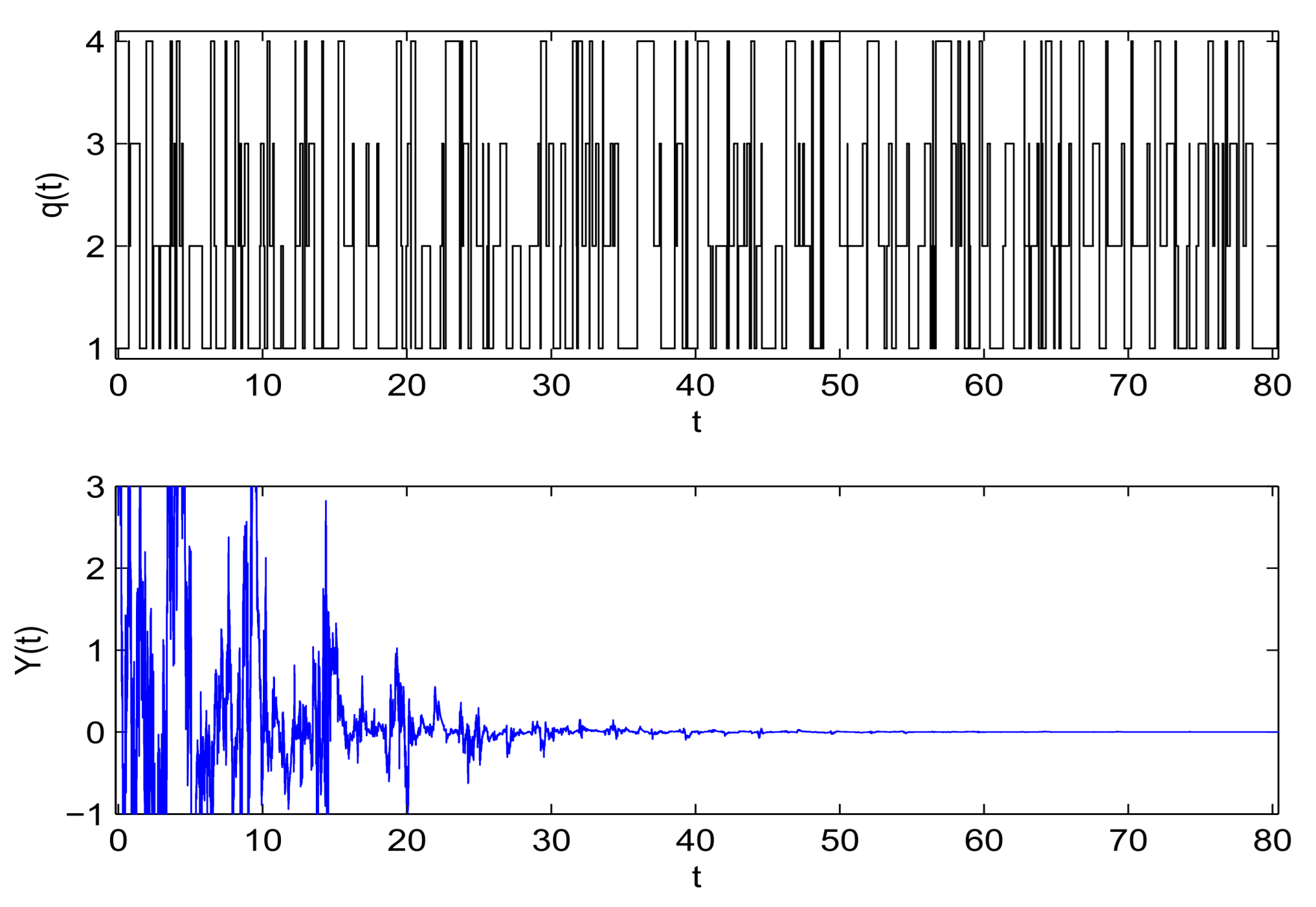
• The final case study uncovers a profound phenomenon: even when a highly nonlinear subsystem exhibits inherent instability, properly designed Markovian switching can induce global stability in the overall hybrid system. This stabilization arises from Markovian switching’s transition probabilities and subsystem dynamics synergistically averaging out unstable modes via ergodicity. This finding significantly enriches the stability theory of nonlinear stochastic systems.
• In this study, we adopt the phase space $C_r$ as our analytical framework, departing from the conventional $BC(-\infty ,0];{\mathbb{R}}^l)$ space commonly employed in stability analysis. This deliberate choice of phase space introduces several technical challenges that demand more sophisticated analytical treatment. Specifically, the $C_r$ space requires the development of new estimation techniques to handle memory-dependent functions, as well as careful consideration of the fading memory properties in stability proofs.

2. Preliminaries

Throughout this paper, unless otherwise specified, we use the following notations. Denote by ${\mathbb{R}}^d$ the d-dimensional Euclidean space and $|·|$ the Euclidean norm. If both $a,b\in \mathbb{R}$, then $a\wedge b=min\{a,b\}$ and $a\vee b=max\{a,b\}$. Let ${\mathbb{R}}_{-}=(-\infty ,0]$ and ${\mathbb{R}}_{+}=[0,\infty )$. If Q is a vector or matrix, its transpose is denoted by $Q^T$. For $Q\in {\mathbb{R}}^{d\times l}$, we let $\left|Q\right|=\sqrt{\mathrm{trace}\left(Q^{T}Q\right)}$ be its Frobenius norm. If Q is a symmetric real-valued matrix ($Q=Q^T$), denote by $Q\le 0$ and $Q<0$ the non-positive and negative definite, respectively. Let $(\Omega ,\mathfrak{F},{\left\{{\mathfrak{F}}_t\right\}}_{t\ge 0},\mathbb{P})$ be a complete probability space with a natural filtration ${\left\{{\mathfrak{F}}_t\right\}}_{t\ge 0}$ satisfying the usual conditions. Let ${\mathbb{1}}_J$ denote the indicator function of the set J. If $Y\left(t\right)$ is an ${\mathbb{R}}^d$-valued stochastic process, define $Y_t=Y_t\left(\theta \right):=\{Y(t+\theta ):-\infty <\theta \le 0\}$ for $t\ge 0$.

Let $W\left(t\right)={(W_1\left(t\right),\dots ,W_l\left(t\right))}^T$ be an l-dimensional Brownian motion defined on the probability space. Let $\mathfrak{q}\left(t\right)$, $t\ge 0$, be a right-continuous Markov chain on the probability space taking values in a finite state space $\mathbb{S}=\{1,2,\dots ,N\}$ with generator $Q={\left({\mathfrak{q}}_{mn}\right)}_{N\times N}$ given by

$$\mathbb{P}\{\mathfrak{q}(t+\Delta )=n|\mathfrak{q}\left(t\right)=m\}=\left\{\begin{array}{cc}{\mathfrak{q}}_{mn}\Delta +o(\Delta ),\hfill & \mathrm{if}m\ne n,\hfill \\ 1+{\mathfrak{q}}_{mn}\Delta +o(\Delta ),\hfill & \mathrm{if}m=n,\hfill \end{array}\right.$$

where $\Delta >0$. Here, ${\mathfrak{q}}_{mn}\ge 0$ is the transition rate from m to n if $m\ne n$ while ${\mathfrak{q}}_{mm}=-{\sum }_{n\ne m}{\mathfrak{q}}_{mn}.$ It is well known that almost all sample paths of $\mathfrak{q}\left(t\right)$ are piecewise constant except for a finite number of simple jumps in any finite subinterval of $R_{+}=[0,\infty )$. We stress that almost all sample paths of $\mathfrak{q}\left(t\right)$ are right continuous. We always assume that the Markov chain $\mathfrak{q}(·)$ is independent of the Brownian motion $W(·)$.

Denote by $C({\mathbb{R}}_{-};{\mathbb{R}}^l)$ the family of continuous functions $\varphi$ from ${\mathbb{R}}_{-}\to {\mathbb{R}}^l$. Let

$$\begin{array}{c}\hfill C_r=\left\{\varphi \in C({\mathbb{R}}_{-};{\mathbb{R}}^l):{\displaystyle \underset{\theta \to -\infty }{lim}}{e}^{r\theta }\varphi \left(\theta \right)\mathrm{exist}\mathrm{in}{\mathbb{R}}^l\right\}.\end{array}$$

(1)

Fading memory space $C_r$ is a Banach space with norm ${\parallel \varphi \parallel }_r={sup}_{\theta \in {\mathbb{R}}_{-}}{e}^{r\theta }\left|\varphi \left(\theta \right)\right|$. Obviously, if $r_1>r_2>0$, we have $C_{r_1}\supseteq C_{r_2}$.

Denote by ${\mathcal{L}}^p\left(C_r\right)$ the space of all $\mathfrak{F}$-measurable $C_r$-valued stochastic process $\varphi$ such that ${\mathbb{E}\parallel \varphi \parallel }_r^p<\infty$. Let ${\mathcal{P}}_0$ denote all probability measures $\nu$ on $(-\infty ,0]$. For any $\epsilon >0$, define

$$\begin{array}{c}\hfill {\mathcal{P}}_{\epsilon }=\left\{\nu \in {\mathcal{P}}_0;{\nu }^{\left(\epsilon \right)}:={\int }_{-\infty }^0{e}^{-\epsilon \theta }\nu \left(d\theta \right)<\infty \right\}.\end{array}$$

(2)

Remark 1.

In practice, there exist numerous probability measures satisfying the aforementioned requirements. Below, we present two representative examples.

(i)

Fix $h>0$ and let δ be the Dirac measure at $-h$ (for the definition of the Dirac measure, see [21], p. 9). Then, for any $\delta \in {\mathcal{P}}_0$ and $\epsilon \ge 0$,

$$\begin{array}{c}\hfill {\delta }^{\left(\epsilon \right)}:={\int }_{-\infty }^0{e}^{-\epsilon \theta }\delta \left(d\theta \right)=e^{\epsilon h}<\infty ,\end{array}$$

(3)

which means that $\delta \in {\mathcal{P}}_{\epsilon }$.

(ii)

Let $\mu \left(d\theta \right)={\epsilon }_0{e}^{{\epsilon }_0\theta }d\theta$. Then, $\mu \in {\mathcal{P}}_0$ and, for any $\epsilon \in (0,{\epsilon }_0)$,

$$\begin{array}{c}\hfill {\mu }^{\left(\epsilon \right)}:={\int }_{-\infty }^0{\epsilon }_0{e}^{-\epsilon \theta }{e}^{{\epsilon }_0\theta }\mu \left(d\theta \right)=\frac{{\epsilon }_0}{{\epsilon }_0-\epsilon }<\infty ,\end{array}$$

(4)

which also means that $\mu \in {\mathcal{P}}_{\epsilon }$ for $\forall \epsilon \in (0,{\epsilon }_0)$.

Let us give a lemma to show that ${\nu }^{\left(\epsilon \right)}$ has the following nice property.

Lemma 1

(c.f. [22], Lemma 1). Fix ${\epsilon }_1>0$. For any $0<\epsilon <{\epsilon }_1$, ${\nu }^{\left(\epsilon \right)}$ is continuously nondecreasing on ε and satisfies ${\nu }^{\left({\epsilon }_1\right)}>{\nu }^{\left(\epsilon \right)}>{\nu }^{\left(0\right)}=1$. Meanwhile, we have ${\mathcal{P}}_{{\epsilon }_1}\subset {\mathcal{P}}_{\epsilon }\subset {\mathcal{P}}_0$.

Let

$$F:C_r\times \mathbb{S}\times {\mathbb{R}}_{+}\to {\mathbb{R}}^d\mathrm{and}G:C_r\times \mathbb{S}\times {\mathbb{R}}_{+}\to {\mathbb{R}}^{d\times l}$$

be both Borel measurable functions. Consider a nonlinear hybrid IMSDE of form

$$\begin{array}{c}\hfill dY\left(t\right)=F(Y_t,\mathfrak{q}\left(t\right),t)dt+G(Y_t,\mathfrak{q}\left(t\right),t)dW\left(t\right),t\ge 0,\end{array}$$

(5)

with the initial data

$$\begin{array}{c}\hfill \xi =\{\varphi \left(\theta \right):\theta \in {\mathbb{R}}_{-}\}\in C_r\mathrm{and}{m}_0\in \mathbb{S},\end{array}$$

(6)

where $Y_t$ is a $C_r$-valued stochastic process.

We impose the following standard local Lipschitz condition and polynomial growth condition on the coefficients F and G:

H1. 

For each positive integer number $k>0$, there is a constant $h_k>0$ such that

$$\begin{array}{c}\hfill |F(\varphi ,m,t)-F(\psi ,m,t)|\vee |G(\varphi ,m,t)-G(\psi ,m,t)|\le h_k{\parallel \varphi -\psi \parallel }_r\end{array}$$

(7)

for all $\varphi ,\psi \in C_r$ with ${\parallel \varphi \parallel }_r\vee {\parallel \psi \parallel }_r\le k$ and all $(m,t)\in \mathbb{S}\times {\mathbb{R}}_{+}$.

H2. 

Assume that there exist positive constants K and $p>1$ such that, for each $(\varphi ,m,t)\in C_r\times \mathbb{S}\times {\mathbb{R}}_{+}$,

$$\begin{array}{cc}\hfill & \left|F(\varphi ,m,t)\right|\le K\left(1+\left|\varphi \left(0\right)\right|+{\int }_{-\infty }^0\left|\varphi \left(\theta \right)\right|{\nu }_1\left(d\theta \right)+{\left|\varphi \left(0\right)\right|}^p+{\int }_{-\infty }^0{\left|\varphi \left(\theta \right)\right|}^p{\nu }_1\left(d\theta \right)\right)\hfill \\ \hfill and\\ \hfill & {\left|G(\varphi ,m,t)\right|}^2\le K\left(1+{\left|\varphi \left(0\right)\right|}^2+{\int }_{-\infty }^0{\left|\varphi \left(\theta \right)\right|}^2{\nu }_2\left(d\theta \right)+{\left|\varphi \left(0\right)\right|}^{p+1}+{\int }_{-\infty }^0{\left|\varphi \left(\theta \right)\right|}^{p+1}{\nu }_2\left(d\theta \right)\right),\hfill \end{array}$$

(8)

where probability measures ${\nu }_1,{\nu }_2\in {\mathcal{P}}_{(p+1)r}$.

Remark 2.

Assumptions (H1) and (H2) are fundamental to the subsequent results. For convenience, they will not be reiterated explicitly in the formulations of the theorems.

Using the standard truncation technique (c.f. [19], Lemma 3.1), we obtain the following result from hypothesis (H1).

Lemma 2.

Under condition (2.5), for any initial data $\xi \in C_r$, Equation (5) has a unique local solution $Y\left(t\right)$ almost surely on $(0,{\rho }_e)$, where ${\rho }_e$ is the potential explosion time.

Considering the impact of infinite memory, we provide moment boundedness and exponential stability conditions for solutions of the hybrid systems while ensuring the existence and uniqueness of the solutions. It should be particularly emphasized that, in contrast to the existing IMSDE literature [19,20], the equations in this paper have different structures under different modes. To illustrate the differences in structure more clearly, we divide the mode set $\mathbb{S}$ into two parts, ${\mathbb{S}}_1=1,\dots ,N_1$ and ${\mathbb{S}}_2=N_1+1,\dots ,N,$ where $1\le N_1<N$. The subsystems of hybrid ISMDE (5) in ${\mathbb{S}}_1$-modes and ${\mathbb{S}}_2$-modes satisfy the classical Khasminskii-type condition and the generalized Khasminskii-type condition, respectively.

Assumption 1.

For $(\varphi ,m,t)\in C_r\times {\mathbb{S}}_1\times {\mathbb{R}}_{+}$, there are real numbers ${\alpha }_m,{\widehat{\alpha }}_m$ and non-negative numbers $c,\widehat{c},{\beta }_{m1},{\beta }_{m2},$${\widehat{\beta }}_{m1},{\widehat{\beta }}_{m2}$ such that, for all

$$\begin{array}{cc}\hfill & \varphi {\left(0\right)}^{T}F(\varphi ,m,t)+\frac{1}{2}{\left|G(\varphi ,m,t)\right|}^2\le c+{\alpha }_m{\left|\varphi \left(0\right)\right|}^2+{\displaystyle \sum _{k=1}^2}{\beta }_{mk}{\int }_{-\infty }^0{\left|\varphi \left(\theta \right)\right|}^2{\nu }_k\left(d\theta \right)\hfill \\ \hfill and\\ \hfill & \varphi {\left(0\right)}^{T}F(\varphi ,m,t)+\frac{p}{2}{\left|G(\varphi ,m,t)\right|}^2\le \widehat{c}+{\widehat{\alpha }}_m{\left|\varphi \left(0\right)\right|}^2+{\displaystyle \sum _{k=1}^2}{\widehat{\beta }}_{mk}{\int }_{-\infty }^0{\left|\varphi \left(\theta \right)\right|}^2{\nu }_k\left(d\theta \right).\hfill \end{array}$$

(9)

For $(\varphi ,m,t)\in C_r\times {\mathbb{S}}_2\times {\mathbb{R}}_{+}$, there are real numbers ${\alpha }_m$ and non-negative numbers $c,{\beta }_{m1},{\beta }_{m2},{\gamma }_m,$${\zeta }_{m1},{\zeta }_{m2}$ such that

$$\begin{array}{cc}\hfill \varphi {\left(0\right)}^{T}F(\varphi ,m,t)+\frac{1}{2}{\left|G(\varphi ,m,t)\right|}^2\le & c+{\alpha }_m{\left|\varphi \left(0\right)\right|}^2+{\displaystyle \sum _{k=1}^2}{\beta }_{mk}{\int }_{-\infty }^0{\left|\varphi \left(\theta \right)\right|}^2{\nu }_k\left(d\theta \right)\hfill \\ \hfill & -{\gamma }_m{\left|\varphi \left(0\right)\right|}^{p+1}+{\displaystyle \sum _{k=1}^2}{\zeta }_{mk}{\int }_{-\infty }^0{\left|\varphi \left(\theta \right)\right|}^{p+1}{\nu }_k\left(d\theta \right).\hfill \end{array}$$

(10)

Assumption 2.

Assuming that the parameters ${\alpha }_1,\cdots ,{\alpha }_N$ and ${\widehat{\alpha }}_1,\cdots ,{\widehat{\alpha }}_{N_1}$ in Assumption (1) make both

$$\begin{array}{c}\hfill M_1:=-2\mathrm{diag}({\alpha }_1,\cdots ,{\alpha }_N)-Q\end{array}$$

and

$$\begin{array}{c}\hfill M_2:=-(p+1)\mathrm{diag}({\widehat{\alpha }}_1,\cdots ,{\widehat{\alpha }}_{N_1})-{\left({\mathfrak{q}}_{mn}\right)}_{m,n\in {\mathbb{S}}_1}\end{array}$$

nonsingular M-matrices.

Remark 3.

Before establishing the stability criteria, we emphasize that Assumption 1 does not require all coefficients ${\alpha }_m$ and ${\widehat{\alpha }}_m$ to be negative. This precisely demonstrates the positive effect of Markovian switching on system stability, a point that will be further verified in the subsequent examples that we provide.

3. Main Result

From the properties of the M-matrix, there exist some positive numbers ${\eta }_m,{\widehat{\eta }}_m(m\in \mathbb{S})$ such that

$$\begin{array}{cc}\hfill & {({\eta }_1,\cdots ,{\eta }_N)}^T:={M_1}^{-1}{(1,\cdots ,1)}^T\mathrm{and}{({\widehat{\eta }}_1,\cdots ,{\widehat{\eta }}_N)}^T:={M_2}^{-1}{(1,\cdots ,1)}^T\hfill \end{array}$$

(11)

hold.

For conciseness in the theorem proofs below, we introduce the following definition:

$$\begin{array}{cc}\hfill {\eta }_{max}& ={\displaystyle \underset{m\in \mathbb{S}}{max}}{\eta }_m,{\eta }_{min}={\displaystyle \underset{m\in \mathbb{S}}{min}}{\eta }_m,{\widehat{\eta }}_{max}={\displaystyle \underset{m\in {\mathbb{S}}_1}{max}}{\widehat{\eta }}_m,{\widehat{\eta }}_{min}={\displaystyle \underset{m\in {\mathbb{S}}_1}{min}}{\widehat{\eta }}_m,\hfill \\ \hfill \kappa & =\frac{2{min}_{m\in S_2}{\gamma }_m{\eta }_m}{1 + {max}_{m\in {\mathbb{S}}_2}{\sum }_{n=1}^{N_1}{\mathfrak{q}}_{mn}{\widehat{\eta }}_n}.\hfill \end{array}$$

(12)

Prior to establishing stability results, we first prove the existence–uniqueness and moment boundedness of solutions under more general conditions.

Theorem 1.

Let Assumptions 1 and 2 hold. Assume also that

$$K_2+K_3<\kappa K_1$$

(13)

holds, where $K_1=1-(p-1){max}_{m\in {\mathbb{S}}_1}{\widehat{\eta }}_m({\widehat{\beta }}_{m1}+{\widehat{\beta }}_{m2}),K_2=\left(2\kappa {max}_{m\in {\mathbb{S}}_1}{\widehat{\eta }}_m{\widehat{\beta }}_{m1}\right)\vee \left(2{max}_{m\in {\mathbb{S}}_2}{\eta }_m{\zeta }_{m1}\right),$ $K_3=\left(2\kappa {max}_{m\in {\mathbb{S}}_1}{\widehat{\eta }}_m{\widehat{\beta }}_{m2}\right)\vee \left(2{max}_{m\in {\mathbb{S}}_2}2{\eta }_m{\zeta }_{m2}\right)$. For any given initial data in Equation (6), Equation (5) has a unique global solution $Y\left(t\right)$ on $t>0$. Moreover, there exists $C>0$ such that

$$\underset{0\le t<\infty }{sup}\mathbb{E}{\left|Y\left(t\right)\right|}^p\le C.$$

(14)

Proof. 

We divide the verification work step by step.

Step 1: Set a function $V:{\mathbb{R}}^d\times \mathbb{S}\to {\mathbb{R}}_{+}$ by

$$\begin{array}{cc}\hfill V\left(\varphi \right(0),m)=& {\eta }_m{\left|\varphi \left(0\right)\right|}^2+\kappa {\widehat{\eta }}_m{\left|\varphi \left(0\right)\right|}^{p+1}{1}_{\{m\in {\mathbb{S}}_1\}},\hfill \end{array}$$

(15)

and define a functional $\mathcal{L}V:C_r\times \mathbb{S}\times {\mathbb{R}}_{+}\to \mathbb{R}$ by

$$\begin{array}{cc}\hfill \mathcal{L}V(\varphi ,m,t)=& V_x(\varphi \left(0\right),m)F(\varphi ,m,t)+\frac{1}{2}\mathrm{trace}\left(G^T(\varphi ,m,t)V_{xx}G(\varphi ,m,t)\right)\hfill \\ \hfill & +{\displaystyle \sum _{n=1}^N}{\mathfrak{q}}_{mn}{\eta }_n{\left|\varphi \left(0\right)\right|}^2+\kappa {\displaystyle \sum _{n=1}^{N_1}}{\mathfrak{q}}_{mn}{\widehat{\eta }}_n{\left|\varphi \left(0\right)\right|}^{p+1}.\hfill \end{array}$$

(16)

For each $i\in {\mathbb{S}}_1$, we get

$$\begin{array}{cc}\hfill \mathcal{L}V(\varphi ,m,t)=& 2{\eta }_m\left({\varphi }^T\left(0\right)F(\varphi ,m,t)+\frac{1}{2}{\left|G(\varphi ,m,t)\right|}^2\right)+{\displaystyle \sum _{n=1}^N}{\mathfrak{q}}_{mn}{\eta }_n{\left|\varphi \left(0\right)\right|}^p\hfill \\ \hfill & +\kappa {\widehat{\eta }}_m{(p+1)\left|\varphi \left(0\right)\right|}^{p-1}{\varphi }^T\left(0\right)F(\varphi ,m,t)+\frac{p+1}{2}\kappa {\widehat{\eta }}_m{\left(\right|\varphi \left(0\right)|}^{p-1}{\left|G(\varphi ,m,t)\right|}^2\hfill \\ \hfill & +{(p-1)\left|\varphi \left(0\right)\right|}^{p-3}|{\varphi }^T\left(0\right)G(\varphi ,m,t){|}^2)+\kappa {\displaystyle \sum _{n=1}^{N_1}}{\mathfrak{q}}_{mn}{\widehat{\eta }}_n{\left|\varphi \left(0\right)\right|}^{p+1}\hfill \\ \hfill \le & 2{\eta }_m\left({\varphi }^T\left(0\right)F(\varphi ,m,t)+\frac{1}{2}{\left|G(\varphi ,m,t)\right|}^2\right)+{\displaystyle \sum _{n=1}^N}{\mathfrak{q}}_{mn}{\eta }_n{\left|\varphi \left(0\right)\right|}^2\hfill \\ \hfill & +(p+1)\kappa {\widehat{\eta }}_m{\left|\varphi \left(0\right)\right|}^{p-1}\left({\varphi }^T\left(0\right)F(\varphi ,m,t)+\frac{p}{2}{\left|G(\varphi ,m,t)\right|}^2\right)\hfill \\ \hfill & +\kappa {\displaystyle \sum _{n=1}^{N_1}}{\mathfrak{q}}_{mn}{\widehat{\eta }}_n{\left|\varphi \left(0\right)\right|}^{p+1}.\hfill \end{array}$$

(17)

Using Assumption 2, we can show that

$$\begin{array}{cc}\hfill \mathcal{L}V(\varphi ,m,t)\le & 2{\eta }_m\left(c+{\alpha }_m{\left|\varphi \left(0\right)\right|}^2+{\displaystyle \sum _{k=1}^2}{\beta }_{mk}{\int }_{-\infty }^0{\left|\varphi \left(\theta \right)\right|}^2{\nu }_k\left(d\theta \right)\right)+{\displaystyle \sum _{n=1}^N}{\mathfrak{q}}_{mn}{\eta }_n{\left|\varphi \left(0\right)\right|}^2\hfill \\ \hfill & +(p+1)\kappa {\widehat{\eta }}_m{\left|\varphi \left(0\right)\right|}^{p-1}\left(\widehat{c}+{\widehat{\alpha }}_m{\left|\varphi \left(0\right)\right|}^2+{\displaystyle \sum _{k=1}^2}{\widehat{\beta }}_{mk}{\int }_{-\infty }^0{\left|\varphi \left(\theta \right)\right|}^2{\nu }_k\left(d\theta \right)\right)\hfill \\ \hfill & +\kappa {\displaystyle \sum _{n=1}^{N_1}}{\mathfrak{q}}_{mn}{\widehat{\eta }}_n{\left|\varphi \left(0\right)\right|}^{p+1}\hfill \\ \hfill \le & 2c{\eta }_m-{\left|\varphi \left(0\right)\right|}^2+2{\eta }_m{\displaystyle \sum _{k=1}^2}{\beta }_{mk}{\int }_{-\infty }^0{\left|\varphi \left(\theta \right)\right|}^2{\nu }_k\left(d\theta \right)\hfill \\ \hfill & +(p+1)\widehat{c}\kappa {\widehat{\eta }}_m{\left|\varphi \left(0\right)\right|}^{p-1}-\kappa \left[1-(p-1){\widehat{\eta }}_m({\widehat{\beta }}_{m1}+{\widehat{\beta }}_{m2})\right]{\left|\varphi \left(0\right)\right|}^{p+1}\hfill \\ \hfill & +2\kappa {\widehat{\eta }}_m{\displaystyle \sum _{k=1}^2}{\widehat{\beta }}_{mk}{\int }_{-\infty }^0{\left|\varphi \left(\theta \right)\right|}^{p+1}{\nu }_k\left(d\theta \right).\hfill \end{array}$$

(18)

For $i\in {\mathbb{S}}_2$, we have

$$\begin{array}{cc}\hfill \mathcal{L}V& (\varphi ,m,t)=2{\eta }_m\left({\varphi }^T\left(0\right)F(\varphi ,m,t)+\frac{1}{2}{\left|G(\varphi ,m,t)\right|}^2\right)\hfill \\ \hfill & +{\displaystyle \sum _{n=1}^N}{\mathfrak{q}}_{mn}{\eta }_n{\left|\varphi \left(0\right)\right|}^2+\kappa {\displaystyle \sum _{n=1}^{N_1}}{\mathfrak{q}}_{mn}{\widehat{\eta }}_n{\left|\varphi \left(0\right)\right|}^{p+1}\hfill \\ \hfill \le & 2{\eta }_m(c+{\alpha }_m{\left|\varphi \left(0\right)\right|}^2+{\displaystyle \sum _{k=1}^2}{\beta }_{mk}{\int }_{-\infty }^0{\left|\varphi \left(\theta \right)\right|}^2{\nu }_k\left(d\theta \right)-{\gamma }_m{\left|\varphi \left(0\right)\right|}^{p+1}\hfill \\ \hfill & +{\displaystyle \sum _{k=1}^2}{\zeta }_{mk}{\int }_{-\infty }^0{\left|\varphi \left(\theta \right)\right|}^{p+1}{\nu }_k\left(d\theta \right))+{\displaystyle \sum _{n=1}^N}{\mathfrak{q}}_{mn}{\eta }_n{\left|\varphi \left(0\right)\right|}^2+\kappa {\displaystyle \sum _{n=1}^{N_1}}{\mathfrak{q}}_{mn}{\widehat{\eta }}_n{\left|\varphi \left(0\right)\right|}^{p+1}\hfill \\ \hfill =& 2c{\eta }_m-{\left|\varphi \left(0\right)\right|}^2+2{\eta }_m{\displaystyle \sum _{k=1}^2}{\beta }_{mk}{\int }_{-\infty }^0{\left|\varphi \left(\theta \right)\right|}^2{\nu }_k\left(d\theta \right)\hfill \\ \hfill & -(2{\gamma }_m{\eta }_m-\kappa {\displaystyle \sum _{n=1}^{N_1}}{\mathfrak{q}}_{mn}{\widehat{\eta }}_n)|\varphi \left(0\right){|}^{p+1}+2{\eta }_m{\displaystyle \sum _{k=1}^2}{\zeta }_{mk}{\int }_{-\infty }^0{\left|\varphi \left(\theta \right)\right|}^{p+1}{\nu }_k\left(d\theta \right).\hfill \end{array}$$

By (12), we can obtain that

$$2{\gamma }_m{\eta }_m-\kappa {\displaystyle \sum _{n=1}^{N_1}}{\mathfrak{q}}_{mn}{\widehat{\eta }}_n\le \kappa .$$

Therefore, we give

$$\begin{array}{cc}\hfill \mathcal{L}V(\varphi ,m,t)\le & 2c{\eta }_m-{\left|\varphi \left(0\right)\right|}^2+2{\eta }_m{\displaystyle \sum _{k=1}^2}{\beta }_{mk}{\int }_{-\infty }^0{\left|\varphi \left(\theta \right)\right|}^2{\nu }_k\left(d\theta \right)\hfill \\ \hfill & -{\kappa \left|\varphi \left(0\right)\right|}^{p+1}+2{\eta }_m{\displaystyle \sum _{k=1}^2}{\zeta }_{mk}{\int }_{-\infty }^0{\left|\varphi \left(\theta \right)\right|}^{p+1}{\nu }_k\left(d\theta \right).\hfill \end{array}$$

(19)

Combining (18) with (19), we could derive that

$$\begin{array}{cc}\hfill \mathcal{L}V& (\varphi ,m,t)\le -\kappa K_1{\left|\varphi \left(0\right)\right|}^{p+1}+K_2{\int }_{-\infty }^0{\left|\varphi \left(\theta \right)\right|}^{p+1}{\nu }_1\left(d\theta \right)+K_3{\int }_{-\infty }^0{\left|\varphi \left(\theta \right)\right|}^{p+1}{\nu }_2\left(d\theta \right)\hfill \\ \hfill & +K_4{\left|\varphi \left(0\right)\right|}^{p-1}-{\left|\varphi \left(0\right)\right|}^2+K_5{\int }_{-\infty }^0{\left|\varphi \left(\theta \right)\right|}^2{\nu }_1\left(d\theta \right)+K_6{\int }_{-\infty }^0{\left|\varphi \left(\theta \right)\right|}^2{\nu }_2\left(d\theta \right)+2c{\eta }_m,\hfill \end{array}$$

(20)

where

$$K_4=(p+1)\kappa \widehat{c}\underset{m\in {\mathbb{S}}_1}{max}{\widehat{\eta }}_m,K_5=2\underset{m\in \mathbb{S}}{max}{\eta }_m{\beta }_{m1},K_6=2\underset{m\in \mathbb{S}}{max}{\eta }_m{\beta }_{m2}.$$

It can be seen from Lemma 1 that, when $\epsilon$ monotonically decreases to 0, ${\nu }_1^{\left(\epsilon \right)}$ and ${\nu }_2^{\left(\epsilon \right)}$ also monotonically decrease to 1. Combining with the continuity of ${\nu }_1^{\left(\epsilon \right)}$ and ${\nu }_2^{\left(\epsilon \right)}$, there exists a ${\epsilon }_2>0$, and the following

$$\begin{array}{c}\hfill \kappa K_1-K_2{\nu }_1^{\left(\epsilon \right)}-K_3{\nu }_2^{\left(\epsilon \right)}>\epsilon \kappa {\widehat{\eta }}_{max}\end{array}$$

(21)

holds for any $\epsilon \in (0,{\epsilon }_2\wedge 2r)$.

Step 2: Since Assumption 7 has shown that IMSDE (5) has a local solution on $t\in (-\infty ,{\rho }_e)$, we just need to show that the solution is global; that is, we need to only prove that ${\rho }_e=\infty$ a.s. Let

$${\rho }_j=inf\{t\in [0,{\rho }_e):|Y\left(t\right)|\ge j\}.$$

Obviously, ${\rho }_j$ is increasing as $j\to \infty$ and ${lim}_{j\to \infty }{\rho }_j={\rho }_{\infty }\le {\rho }_e$ a.s. If we can show that ${\rho }_{\infty }=\infty$ a.s., then ${\rho }_e=\infty$ a.s., which implies the desired result. This is also equivalent to proving that there is ${lim}_{j\to \infty }\mathbb{P}({\rho }_j\le t)\to 0$ for any $t>0$.

By applying the generalized Itô formula (c.f. [23], Lemma 1.9) to $e^{\epsilon t}V$, we get

$$\begin{array}{cc}\hfill e^{\epsilon (t\wedge {\rho }_j)}& V(Y(t\wedge {\rho }_j),\mathfrak{q}(t\wedge {\rho }_j))-V(y\left(0\right),m_0)=\hfill \\ \hfill & {\int }_0^{t\wedge {\rho }_j}{e}^{\epsilon w}[\epsilon V(Y\left(w\right),\mathfrak{q}\left(w\right))+\mathcal{L}V(Y_w,\mathfrak{q}\left(w\right),w)]dw+M\left(t\right),\hfill \end{array}$$

(22)

where $M\left(t\right)$ is a local martingale with the initial value $M\left(0\right)=0$. Take the expectation on both sides of (22). We then derive from (18) that

$$\begin{array}{cc}\hfill \mathbb{E}& e^{\epsilon (t\wedge {\rho }_j)}V(Y(t\wedge {\rho }_j),\mathfrak{q}(t\wedge {\rho }_j))-V(Y\left(0\right),m_0)\hfill \\ \hfill =& \mathbb{E}{\int }_0^{t\wedge {\rho }_j}{e}^{\epsilon w}\left[\epsilon {\eta }_m{\left|Y\left(w\right)\right|}^2+\epsilon \kappa {\widehat{\eta }}_m{\left|Y\left(w\right)\right|}^{p+1}{\mathbb{1}}_{\{m\in {\mathbb{S}}_1\}}+\mathcal{L}V(Y_w,\mathfrak{q}\left(w\right),w)\right]dw\hfill \\ \hfill \le & -(\kappa K_1-\epsilon \kappa {\widehat{\eta }}_m)\mathbb{E}{\int }_0^{t\wedge {\rho }_j}{e}^{\epsilon w}|Y\left(w\right){|}^{p+1}dw+K_2\mathbb{E}{\int }_0^{t\wedge {\rho }_j}{e}^{\epsilon w}{\int }_{-\infty }^0{\left|Y(w+\theta )\right|}^{p+1}{\nu }_1\left(d\theta \right)dw\hfill \\ \hfill & +K_3\mathbb{E}{\int }_0^{t\wedge {\rho }_j}{e}^{\epsilon w}{\int }_{-\infty }^0{\left|Y(w+\theta )\right|}^{p+1}{\nu }_2\left(d\theta \right)dw+\mathbb{E}{\int }_0^{t\wedge {\rho }_j}{e}^{\epsilon w}{K}_4{\left|Y\left(w\right)\right|}^{p-1}dw\hfill \\ \hfill & -(1-\epsilon {\eta }_m)\mathbb{E}{\int }_0^{t\wedge {\rho }_j}{e}^{\epsilon w}|Y\left(w\right){|}^{2}dw+K_5\mathbb{E}{\int }_0^{t\wedge {\rho }_j}{e}^{\epsilon w}{\int }_{-\infty }^0{\left|Y(w+\theta )\right|}^2{\nu }_1\left(d\theta \right)dw\hfill \\ \hfill & +K_6\mathbb{E}{\int }_{-\infty }^0{\left|Y(w+\theta )\right|}^2{\nu }_2\left(d\theta \right)dw+\mathbb{E}{\int }_0^{t\wedge {\rho }_j}2c{\eta }_m{e}^{\epsilon w}dw.\hfill \end{array}$$

(23)

By the Fubini theorem and a substitution technique, we get

$$\begin{array}{cc}\hfill {\int }_0^{t\wedge {\rho }_j}& e^{\epsilon w}dw{\int }_{-\infty }^0{\left|Y(w+\theta )\right|}^{p+1}{\nu }_k\left(d\theta \right)\hfill \\ \hfill =& {\int }_0^{t\wedge {\rho }_j}{e}^{\epsilon w}dw{\int }_{-\infty }^{-w}{\left|Y(w+\theta )\right|}^{p+1}{\nu }_k\left(d\theta \right)+{\int }_0^{t\wedge {\rho }_j}{e}^{\epsilon w}dw{\int }_{-w}^0{\left|Y(w+\theta )\right|}^{p+1}{\nu }_k\left(d\theta \right)\hfill \\ \hfill =& {\int }_0^{t\wedge {\rho }_j}{e}^{\epsilon w}dw{\int }_{-\infty }^{-w}{e}^{(p+1)r(w+\theta )}{\left|Y(w+\theta )\right|}^{p+1}{e}^{-(p+1)r(w+\theta )}{\nu }_k\left(d\theta \right)\hfill \\ \hfill & +{\int }_{-t\wedge {\rho }_j}^0{e}^{-\epsilon \theta }{\nu }_k\left(d\theta \right){\int }_{-\theta }^{t\wedge {\rho }_j}{e}^{\epsilon (w+\theta )}{\left|Y(w+\theta )\right|}^{p+1}dw\hfill \\ \hfill \le & {\parallel \varphi \parallel }_r^{p+1}{\int }_0^{t\wedge {\rho }_j}{e}^{\epsilon w-(p+1)rw}dw{\int }_{-\infty }^{-w}{e}^{-(p+1)r\theta }{\nu }_k\left(d\theta \right)\hfill \\ \hfill & +{\int }_{-\infty }^0{e}^{-\epsilon \theta }{\nu }_k\left(d\theta \right){\int }_0^{t\wedge {\rho }_j}{e}^{\epsilon w}{\left|y\left(w\right)\right|}^{p+1}dw\hfill \\ \hfill \le & \frac{1}{(p+1)r-\epsilon }{\parallel \varphi \parallel }_r^{p+1}{\nu }_k^{\left(\right(p+1\left)r\right)}+{\nu }_k^{\left(\epsilon \right)}{\int }_0^{t\wedge {\rho }_j}{e}^{\epsilon w}{\left|Y\left(w\right)\right|}^{p+1}dw\hfill \\ \hfill \le & \frac{1}{(p+1)r-\epsilon }{\parallel \varphi \parallel }_r^{p+1}{\nu }_k^{\left(\right(p+1\left)r\right)}+{\nu }_k^{\left(\right(p+1\left)r\right)}{\int }_0^{t\wedge {\rho }_j}{e}^{\epsilon w}{\left|Y\left(w\right)\right|}^{p+1}dw.\hfill \end{array}$$

Similarly,

$$\begin{array}{cc}\hfill {\int }_0^{t\wedge {\rho }_j}& e^{\epsilon w}dw{\int }_{-\infty }^0{\left|Y(w+\theta )\right|}^2{\nu }_k\left(d\theta \right)\hfill \\ \hfill =& {\int }_0^{t\wedge {\rho }_j}{e}^{\epsilon w}dw{\int }_{-\infty }^{-w}{\left|Y(w+\theta )\right|}^2{\nu }_k\left(d\theta \right)+{\int }_0^{t\wedge {\rho }_j}{e}^{\epsilon w}dw{\int }_{-w}^0{\left|Y(w+\theta )\right|}^2{\nu }_k\left(d\theta \right)\hfill \\ \hfill =& {\int }_0^{t\wedge {\rho }_j}{e}^{\epsilon w}dw{\int }_{-\infty }^{-w}{e}^{2r(w+\theta )}{\left|Y(w+\theta )\right|}^2{e}^{-2r(w+\theta )}{\nu }_k\left(d\theta \right)\hfill \\ \hfill & +{\int }_{-t\wedge {\rho }_j}^0{e}^{-\epsilon \theta }{\nu }_k\left(d\theta \right){\int }_{-\theta }^{t\wedge {\rho }_j}{e}^{\epsilon (w+\theta )}{\left|Y(w+\theta )\right|}^{2}dw\hfill \\ \hfill \le & {\parallel \varphi \parallel }_r^2{\int }_0^{t\wedge {\rho }_j}{e}^{\epsilon w-2rw}dw{\int }_{-\infty }^{-w}{e}^{-2r\theta }{\nu }_k\left(d\theta \right)+{\int }_{-\infty }^0{e}^{-\epsilon \theta }{\nu }_k\left(d\theta \right){\int }_0^{t\wedge {\rho }_j}{e}^{\epsilon w}{\left|Y\left(w\right)\right|}^{2}dw\hfill \\ \hfill \le & \frac{1}{2r-\epsilon }{\parallel \varphi \parallel }_r^2{\nu }_k^{\left(2r\right)}+{\nu }_k^{\left(\epsilon \right)}\mathbb{E}{\int }_0^{t\wedge {\rho }_j}{e}^{\epsilon w}{\left|Y\left(w\right)\right|}^{2}dw\hfill \\ \hfill \le & \frac{1}{2r-\epsilon }{\parallel \varphi \parallel }_r^2{\nu }_k^{\left(2r\right)}+{\nu }_k^{\left(2r\right)}\mathbb{E}{\int }_0^{t\wedge {\rho }_j}{e}^{\epsilon w}{\left|Y\left(w\right)\right|}^{2}dw.\hfill \end{array}$$

Substituting these into (23), we have

$$\begin{array}{cc}\hfill {\eta }_{min}\mathbb{E}{e}^{\epsilon (t\wedge {\rho }_j)}{\left|Y(t\wedge {\rho }_j)\right|}^2\le & C_1+\mathbb{E}{\int }_0^{t\wedge {\rho }_j}{e}^{\epsilon w}(-{\widehat{K}}_1{\left|Y\left(w\right)\right|}^{p+1}+K_4{\left|Y\left(w\right)\right|}^{p-1}\hfill \\ \hfill & -(1-K_5{\nu }_1^{\left(\epsilon \right)}-K_6{\nu }_2^{\left(\epsilon \right)}-\epsilon {\eta }_{max}){\left|Y\left(w\right)\right|}^2+2c{\eta }_{max})dw,\hfill \end{array}$$

(24)

where

$$\begin{array}{cc}\hfill {\widehat{K}}_1=& \kappa K_1-K_2{\nu }_1^{\left(\epsilon \right)}-K_3{\nu }_2^{\left(\epsilon \right)}-\epsilon \kappa {\widehat{\eta }}_{max},\hfill \\ \hfill C_1=& V(Y\left(0\right),m_0)+{\parallel \varphi \parallel }_r^{p+1}\frac{K_2{\nu }_1^{\left(\right(p+1\left)r\right)}+K_3{\nu }_2^{\left(\right(p+1\left)r\right)}}{(p+1)r-\epsilon }\hfill \\ \hfill & +{\widehat{\eta }}_{max}{\left|Y\left(0\right)\right|}^{p+1}+{\parallel \varphi \parallel }_r^2\frac{K_5{\nu }_1^{\left(2r\right)}+K_6{\nu }_2^{\left(2r\right)}}{(2r-\epsilon )}+{\eta }_{max}{\left|Y\left(0\right)\right|}^2.\hfill \end{array}$$

Recalling (21), we get ${\widehat{K}}_1>0$. This yields that

$$\begin{array}{c}\hfill {\eta }_{min}\mathbb{E}{e}^{\epsilon (t\wedge {\rho }_j)}{\left|Y(t\wedge {\rho }_j)\right|}^p\le C_1+C_2{e}^{\epsilon t},\end{array}$$

(25)

where

$$C_2=-{\widehat{K}}_1{\left|s\right|}^{p+1}+K_4{\left|s\right|}^{p-1}-(1-K_5{\nu }_1^{\left(\epsilon \right)}-K_6{\nu }_2^{\left(\epsilon \right)}-\epsilon {\eta }_{max}){\left|s\right|}^2+2c{\eta }_{max}.$$

Choosing $t=T>0$ gives

$$\begin{array}{cc}\hfill j^p{\eta }_{min}\mathbb{P}({\rho }_j\le T)\le & {\eta }_{min}{\mathbb{E}\left\{\right|Y\left(T\right)|}^p{\mathbb{1}}_{{\rho }_j\le T}\}+{\eta }_{min}\mathbb{E}\left\{j^p{\mathbb{1}}_{{\rho }_j\le T}\right\}\hfill \\ \hfill =& {\eta }_{min}\mathbb{E}{\left|Y(T\wedge {\rho }_j)\right|}^p\hfill \\ \hfill \le & {\eta }_{min}\mathbb{E}{e}^{\epsilon (T\wedge {\rho }_j)}{\left|Y(t\wedge {\rho }_j)\right|}^p\hfill \\ \hfill \le & C_1+C_2{e}^{\epsilon T},\hfill \end{array}$$

Then, we have

$$\begin{array}{c}\hfill \mathbb{P}({\rho }_j\le T)\le \frac{C_1+C_2{e}^{\epsilon T}}{j^p{\eta }_{min}}.\end{array}$$

Letting $j\to \infty$, we obtain that $\mathbb{P}({\rho }_{\infty }\le T)=0$, namely,

$$\mathbb{P}({\rho }_{\infty }>T)=1.$$

Since $T\ge 0$ is arbitrary, we must have $\mathbb{P}({\rho }_{\infty }=\infty )=1$, as required. This completes the proof, demonstrating that (5) admits a global solution $Y\left(t\right)$ on $[0,\infty )$.

Step 3: Letting $j\to \infty$, we obtain from (25) that

$$\begin{array}{c}\hfill {\eta }_{min}{e}^{\epsilon t}\mathbb{E}{\left|Y\left(t\right)\right|}^p\le C_1+C_2{e}^{\epsilon t}.\end{array}$$

As a result,

$$\begin{array}{c}\hfill {\mathbb{E}\left|Y\left(t\right)\right|}^p\le \frac{C_1}{{\eta }_{min}{e}^{\epsilon t}}+\frac{C_2}{{\eta }_{min}}\le C.\end{array}$$

Putting $C={sup}_{s\ge 0}\left\{\frac{C_1}{{\eta }_{min}{e}^{\epsilon s}}+\frac{C_2}{{\eta }_{min}}\right\}<\infty$, we obtain the desired result of item (14). □

Remark 4.

In the proof of Theorem 1 regarding the existence and uniqueness of solutions, we apply the generalized Itô formula to $e^{\epsilon t}V$ rather than to V directly. This modification serves to streamline the proof while preserving its essential structure, though at the expense of requiring stronger conditions on the probability measure ${\mathcal{P}}_{\epsilon }$ in the existence and uniqueness argument.

Theorem 2.

Let the assumptions of Theorem 1 hold, with the additional requirement that $c=\widehat{c}=0$ in Conditions (9) and (10). Furthermore, these assume that

$$K_5+K_6<1.$$

(26)

Thus, (i) the solution of Equation (5) satisfies

$$\underset{t\to \infty }{lim\; sup}\frac{1}{t}{log\left(\mathbb{E}\right|Y\left(t\right)|}^2)<0.$$

(27)

That is, Equation (5) is mean square exponential stability.

(ii) The solution of Equation (5) satisfies

$$\underset{t\to \infty }{lim\; sup}\frac{1}{t}log\left(\right|Y\left(t\right)\left|\right)<0,a.s.$$

(28)

That is, Equation (5) is almost surely exponentially stable.

Proof. 

(i) Recalling Condition (26), similar to the discussion of Theorem 1, there exists a ${\epsilon }_3>0$, which shows that

$$\begin{array}{c}\hfill \widehat{K_2}:=1-K_5{\nu }_1^{\left(\epsilon \right)}-K_6{\nu }_2^{\left(\epsilon \right)}-\epsilon {\eta }_{max}>0\end{array}$$

(29)

for any $\epsilon \in (0,{\epsilon }_3\wedge 2r)$. Substituting these into (24), and recalling $K_4=c=0$, we have

$$\begin{array}{cc}\hfill {\eta }_{min}\mathbb{E}{e}^{\epsilon (t\wedge {\rho }_j)}{\left|Y(t\wedge {\rho }_j)\right|}^2\le & C_1+\mathbb{E}{\int }_0^{t\wedge {\rho }_j}{e}^{\epsilon w}\left(-{\widehat{K}}_1{\left|Y\left(w\right)\right|}^{p+1}-{\widehat{K}}_2{\left|Y\left(w\right)\right|}^2\right)dw\hfill \\ \hfill \le & C_1\hfill \end{array}$$

Letting $j\to \infty$ yields

$$\begin{array}{c}\hfill {\eta }_{min}{e}^{\epsilon t}\mathbb{E}{\left|Y\left(t\right)\right|}^2\le C_1.\end{array}$$

As a result,

$$\begin{array}{c}\hfill \underset{t\to \infty }{lim\; sup}\frac{1}{t}{log\left(\mathbb{E}\right|Y\left(t\right)|}^2)\le -\epsilon ,\end{array}$$

which means the desired assertion (28).

(ii) To show (29), similar to the discussion of Theorem 1, we get

$$\begin{array}{cc}\hfill e^{\epsilon t}V(Y\left(t\right),\mathfrak{q}\left(t\right))=& V(Y\left(0\right),m_0)+{\int }_0^t{e}^{\epsilon w}\left[\epsilon V(Y\left(w\right),\mathfrak{q}\left(w\right))+\mathcal{L}V(Y_w,\mathfrak{q}\left(w\right),w)\right]dw+M\left(t\right)\hfill \\ \hfill \le & C_1-{\widehat{K}}_1{\int }_0^t{e}^{\epsilon w}{\left|Y\left(w\right)\right|}^{p+1}dw-{\widehat{K}}_2{\int }_{-\infty }^t{e}^{\epsilon w}{\left|Y\left(w\right)\right|}^{2}dw+M\left(t\right).\hfill \end{array}$$

Using (14), (22) and (27), we then derive that

$$\begin{array}{cc}\hfill {\eta }_{min}& e^{\epsilon t}{\left|Y\left(t\right)\right|}^2\le C_1+M\left(t\right).\hfill \end{array}$$

By the non-negative semi-martingale convergence theorem (c.f. [24], Theorem 1.10), we have

$$\begin{array}{c}\hfill {\displaystyle \underset{t\to \infty }{lim\; sup}}{e}^{\epsilon t}{\left|Y\left(t\right)\right|}^2<\infty ,a.s.\end{array}$$

which is the desired result (29). The proof is complete. □

4. Example

To illustrate the effectiveness of our given theory clearly, in this section, we consider the following one-dimensional IMSDE:

$$\begin{array}{cc}\hfill dY\left(t\right)=& F(Y_t,\mathfrak{q}\left(t\right),t)dt+G(Y_t,\mathfrak{q}\left(t\right),t)dW\left(t\right),\hfill \end{array}$$

(30)

in which the coefficients are defined by

$$\begin{array}{c}\hfill F(Y_t,m,t)=\left\{\begin{array}{cc}-3.2Y\left(t\right),\hfill & \mathrm{if}m=1,\hfill \\ -4.7Y\left(t\right),\hfill & \mathrm{if}m=2,\hfill \\ -Y\left(t\right)\left(3Y^2\left(t\right)+0.4{\int }_{-\infty }^0{Y}^2(t+\theta ){\nu }_1\left(d\theta \right)-0.5\right),\hfill & \mathrm{if}m=3,\hfill \\ -Y\left(t\right)\left(6Y^2\left(t\right)-0.8{\int }_{-\infty }^0{Y}^2(t+\theta ){\nu }_1\left(d\theta \right)+4\right),\hfill & \mathrm{if}m=4.\hfill \end{array}\right.\end{array}$$

(31)

and

$$\begin{array}{c}\hfill G(Y_t,m,t)=\left\{\begin{array}{cc}1.5{\int }_{-\infty }^{0}Y(t+\theta ){\nu }_2\left(d\theta \right),\hfill & \mathrm{if}m=1,\hfill \\ 1.8{\int }_{-\infty }^{0}Y(t+\theta ){\nu }_2\left(d\theta \right),\hfill & \mathrm{if}m=2,\hfill \\ 1.2(Y\left(t\right)+{\int }_{-\infty }^0|Y(t+\theta ){|}^{3/2}{\nu }_2\left(d\theta \right)),\hfill & \mathrm{if}m=3,\hfill \\ 2.8{\int }_{-\infty }^0{\left|Y(t+\theta )\right|}^{3/2}{\nu }_2\left(d\theta \right),\hfill & \mathrm{if}m=4.\hfill \end{array}\right.\end{array}$$

(32)

$q\left(t\right)\in \mathbb{S}=\{1,2,3,4\}$ is a Markov chain with its generator

$$Q=\left(\begin{array}{cccc}-5& 1& 1& 3\\ 1& -6& 3& 2\\ 5& 6& -15& 4\\ 1& 4& 2& -7\end{array}\right).$$

(33)

Obviously, Equation (30) satisfies Assumptions (H1) and (H2), and ${\mathbb{S}}_1=\{1,2\}$, ${\mathbb{S}}_2=\{3,4\}$. For $(Y_t,m,t)\in C_r\times {\mathbb{S}}_1\times {\mathbb{R}}_{+}$, we have

$$\begin{array}{c}\hfill Y\left(t\right)F(Y_t,m,t)+\frac{1}{2}{\left|G(Y_t,m,t)\right|}^2\le \left\{\begin{array}{cc}-3.2Y^2\left(t\right)+1.125{\int }_{-\infty }^0{Y}^2(t+\theta ){\nu }_2\left(d\theta \right),& \mathrm{if}m=1,\hfill \\ -4.7Y^2\left(t\right)+1.62{\int }_{-\infty }^0{Y}^2(t+\theta ){\nu }_2\left(d\theta \right),& \mathrm{if}m=2,\hfill \end{array}\right.\end{array}$$

and

$$\begin{array}{c}\hfill Y\left(t\right)F(Y_t,m,t)+\frac{p}{2}{\left|G(Y_t,m,t)\right|}^2\le \left\{\begin{array}{cc}-3.2Y^2\left(t\right)+3.375{\int }_{-\infty }^0{Y}^2(t+\theta ){\nu }_2\left(d\theta \right),& \mathrm{if}m=1,\hfill \\ -4.7Y^2\left(t\right)+4.86{\int }_{-\infty }^0{Y}^2(t+\theta ){\nu }_2\left(d\theta \right),& \mathrm{if}m=2.\hfill \end{array}\right.\end{array}$$

For $(Y_t,m,t)\in C_r\times {\mathbb{S}}_2\times {\mathbb{R}}_{+}$, we have

$$\begin{array}{cc}\hfill Y\left(t\right)& F(Y_t,m,t)+\frac{1}{2}{\left|G(Y_t,m,t)\right|}^2\hfill \\ \hfill & \le \left\{\begin{array}{c}1.94Y^2\left(t\right)+0.72{\int }_{-\infty }^0{Y}^2(t+\theta ){\nu }_2\left(d\theta \right)\\ -3Y^4\left(t\right)+0.72{\int }_{-\infty }^0{Y}^4(t+\theta ){\nu }_2\left(d\theta \right),& \mathrm{if}m=3,\hfill \\ -4Y^2\left(t\right)+1.4{\int }_{-\infty }^0{Y}^2(t+\theta ){\nu }_2\left(d\theta \right)-5.6Y^4\left(t\right)\\ +0.4{\int }_{-\infty }^0{Y}^4(t+\theta ){\nu }_1\left(d\theta \right))+1.4{\int }_{-\infty }^0{Y}^4(t+\theta ){\nu }_2\left(d\theta \right)),& \mathrm{if}m=4,\hfill \end{array}\right.\hfill \end{array}$$

which implies that

$${\alpha }_1=-3.2,{\alpha }_2=-4.7,{\alpha }_3=1.94,{\alpha }_4=-4,{\widehat{\alpha }}_1=-3.2,{\widehat{\alpha }}_2=-4.7.$$

Hence,

$${\mathcal{M}}_1=\left(\begin{array}{cccc}11.4& -1& -1& -3\\ -1& 15.4& -3& -2\\ -5& -6& -11.12& -4\\ -1& -4& -2& -15\end{array}\right)\mathrm{and}{\mathcal{M}}_2=\left(\begin{array}{cc}17.8& -1\\ -1& 24.8\end{array}\right)$$

are both nonsingular M-matrices; that is, Assumption 2 also holds. Recalling (11) and (12), we have

$$\begin{array}{cc}\hfill {\eta }_1& =0.171163,{\eta }_2=0.157363,{\eta }_3=0.309838,{\eta }_4=0.161352,\hfill \\ \hfill {\widehat{\eta }}_1& =0.058578,{\widehat{\eta }}_2=0.042685,\kappa =1.20015.\hfill \end{array}$$

By simple calculation, we get

$$\begin{array}{cc}\hfill K_2+K_3& =0.627018<0.702215=\kappa K_1,\hfill \\ \hfill K_5+K_6& =0.509855<1,\hfill \end{array}$$

which means that conditions (30) and (27) also hold. By Theorem 2, Equation (30) is exponentially stable in $L^2$ and almost surely as well. Letting $d{\nu }_1\left(\theta \right)=e^{\theta }d\theta$ on $\theta \in (-\infty ,0]$, ${\nu }_2\left(\theta \right)$ be the Dirac measure at $-100$, the initial value

$$\begin{array}{c}\hfill \xi =\left\{\begin{array}{cc}5e^{0.01\theta }-5e^{-1},& \mathrm{if}\theta \in (-100,0],\hfill \\ 0,& \mathrm{if}\theta \in (-\infty ,-100]\hfill \end{array}\right.\mathrm{and}{m}_0=1.\end{array}$$

(34)

The numerical simulation in Figure 1 shows that Equation (30) is almost surely exponentially stable.

Remark 5.

Equation (30) is widely discussed in population dynamics (see, e.g., [5,23,25] and the references therein). Since the numerical simulation of systems with infinite delay is challenging, we adopt a specific initial condition (34). Nevertheless, this choice suffices to demonstrate our theoretical findings. For further details on numerical methods for IMSDEs, we refer to [17].

Remark 6.

In this example, we can see that ${\xi }_{10}=1>0$ in mode 3 and Theorem 3 in Hu et al.’s work [22] are invalid here. Under the same distribution and initial conditions as in Figure 2, the numerical simulation in Figure 2 shows that mode 3 of (30) is unstable. However, by incorporating the Markov chain’s influence and employing the M-matrix methodology, the complete system satisfies Conditions (13) and (27), which consequently endows our results with greater generality.

5. Conclusions

This paper has investigated the structural stability of hybrid stochastic differential equations with infinite memory, focusing on systems whose coefficients exhibit superlinear growth. By employing M-matrices, we have revealed the positive role of the transition probability matrix in Markovian switching on the stability of switched stochastic systems. These results have extended the stability criteria for stochastic differential equations with infinite memory. Finally, numerical simulations have successfully supported our theoretical results.

In this paper, we discuss the exponential stability of the system. Further studies could explore the system’s stability in a broader sense (such as polynomial stability, stability in distribution, etc.). Additionally, the results of this paper can be applied to stochastic differential equations with Lévy noise or those driven by G-Brownian motion. Finally, based on the findings presented here, the feedback control problem for such IMSDEs could be investigated.

References

1. Guedda, L.; Raynaud de Fitte, P. Existence and dependence results for semilinear functional stochastic differential equations with infinite delay in a Hilbert space. Mediterr. J. Math. 2016, 13, 4153–4174. [Google Scholar] [CrossRef]
2. Shi, B.; Mao, X.; Wu, F. Stabilisation with general decay rate by delay feedback control for nonlinear neutral stochastic functional differential equations with infinite delay. Syst. Control Lett. 2023, 172, 105435. [Google Scholar] [CrossRef]
3. Wang, L.; Li, J. Asymptotic Bismut formula for Lions derivative of McKean-Vlasov neutral stochastic differential equations with infinite memory. Commun. Pure Appl. Anal. 2025, 24, 1118–1139. [Google Scholar] [CrossRef]
4. Yao, X.; You, S.; Mao, W.; Mao, X. On the decay rate for a stochastic delay differential equation with an unbounded delay. Appl. Math. Lett. 2025, 166, 109541. [Google Scholar] [CrossRef]
5. Lu, C. Dynamics of a stochastic Markovian switching predator–prey model with infinite memory and general Lévy jumps. Math. Comput. Simul. 2021, 181, 316–332. [Google Scholar] [CrossRef]
6. Lu, B.; Zhu, Q.; He, P. Exponential stability of highly nonlinear hybrid differently structured neutral stochastic differential equations with unbounded delays. Fractal Fract. 2022, 6, 385. [Google Scholar] [CrossRef]
7. Zhao, S.f. On β-extinction and stability of a stochastic Lotka-Volterra system with infinite delay. Acta Math. Appl. Sin. 2024, 40, 1045–1059. [Google Scholar] [CrossRef]
8. Liu, L.; Zhang, Y.; Tian, Y.; Wei, D.; Huang, Z. Sliding mode control for stochastic SIR models with telegraph and Lévy noise: Theory and applications. Symmetry 2025, 17, 963. [Google Scholar] [CrossRef]
9. Hu, L.; Mao, X.; Zhang, L. Robust stability and boundedness of nonlinear hybrid stochastic differential delay equations. IEEE Trans. Autom. Control 2013, 58, 2319–2332. [Google Scholar] [CrossRef]
10. Fei, W.; Hu, L.; Mao, X.; Shen, M. Structured robust stability and boundedness of nonlinear hybrid delay systems. SIAM J. Control Optim. 2018, 56, 2662–2689. [Google Scholar] [CrossRef]
11. Shen, M.; Mei, C.; Deng, S. Analysis on structured stability of highly nonlinear pantograph stochastic differential equations. Syst. Sci. Control Eng. 2019, 7, 54–64. [Google Scholar] [CrossRef]
12. Lu, B.; Song, R.; Zhu, Q. Exponential stability of highly nonlinear hybrid NSDEs with multiple time-Dependent delays and different structures and the Euler-Maruyama method. J. Frankl. Inst. 2022, 359, 2283–2316. [Google Scholar] [CrossRef]
13. Xu, H.; Mao, X. Structured stabilisation of superlinear delay systems by bounded discrete-time state feedback control. Automatica 2024, 159, 111409. [Google Scholar] [CrossRef]
14. Shi, B.; Mao, X.; Wu, F. Stabilisation of hybrid system with different structures by feedback control based on discrete-time state observations. Nonlinear Anal. Hybrid Syst. 2022, 45, 101198. [Google Scholar] [CrossRef]
15. Hino, Y.; Murakami, S.; Naito, T. Functional Differential Equations with Infinite Delay; Springer: Berlin/Heidelberg, Germany, 1991. [Google Scholar]
16. Mei, C.; Fei, C.; Fei, W.; Mao, X. Exponential stabilization by delay feedback control for highly nonlinear hybrid stochastic functional differential equations with infinite delay. Nonlinear Anal. Hybrid Syst. 2021, 40, 101026. [Google Scholar] [CrossRef]
17. Li, G.; Li, X.; Mao, X.; Song, G. Hybrid stochastic functional differential equations with infinite delay: Approximations and numerics. J. Differ. Equ. 2023, 374, 154–190. [Google Scholar] [CrossRef]
18. Zhao, L.; Fan, Q. Delay feedback control based on discrete-time state observations for highly nonlinear hybrid stochastic functional differential equations with infinite delay. Int. J. Control. Autom. Syst. 2024, 22, 560–570. [Google Scholar] [CrossRef]
19. Wu, F.; Yin, G.; Mei, H. Stochastic functional differential equations with infinite delay: Existence and uniqueness of solutions, solution maps, Markov properties, and ergodicity. J. Differ. Equ. 2017, 262, 1226–1252. [Google Scholar] [CrossRef]
20. Zhen, Y.; Xi, F. Numerical solutions of regime-switching functional diffusions with infinite delay. Stoch. Model. 2024, 40, 617–633. [Google Scholar] [CrossRef]
21. Kallenberg, O. Foundations of Modern Probability; Springer: New York, NY, USA, 2006. [Google Scholar]
22. Hu, Y.; Wu, F.; Huang, C. Robustness of exponential stability of a class of stochastic functional differential equations with infinite delay. Automatica 2009, 45, 2577–2584. [Google Scholar] [CrossRef]
23. Mao, X.; Yuan, C. Stochastic Differential Equations with Markovian Switching; Imperial College Press: London, UK, 2006. [Google Scholar]
24. Mao, X. Stochastic Differential Equations and Applications, 2nd ed.; Horwood Publishing: Chichester, UK, 2007. [Google Scholar]
25. Zhang, M.; Zhu, Q.; Tian, J. Convergence rates of partial truncated numerical algorithm for stochastic age-dependent cooperative Lotka–Volterra system. Symmetry 2024, 16, 1659. [Google Scholar] [CrossRef]
Figure 1. The computer simulation of the sample paths of the Markov chain and Equation (30) using the Euler–Maruyama method with step size 10 3 .
Symmetry 17 01077 g001
Figure 2. The computer simulation of the sample paths of the Markov chain and mode 3 of Equation (30) using the Euler–Maruyama method with step size 10 3 .
Symmetry 17 01077 g002
Disclaimer/Publisher’s Note: The statements, opinions and data contained in all publications are solely those of the individual author(s) and contributor(s) and not of MDPI and/or the editor(s). MDPI and/or the editor(s) disclaim responsibility for any injury to people or property resulting from any ideas, methods, instructions or products referred to in the content.