
Fault Diagnosis Method for Pumped Storage Units Based on VMD-BILSTM

Abstract
1. Introduction
2. Fundamental Theory
2.1. Variational Mode Decomposition
- (1)
- Initialize the parameters , and , set the iteration loop , and update the parameters iteratively according to Equations (2) and (3).
- (2)
- Update .
- (3)
- Update .
- (4)
- Update .
- (5)
- Convergence determination.
- (6)
- Check whether the iteration condition is satisfied; otherwise, return to step (2).
2.2. Subtractive Average Optimizer Improved by Multiple Strategies
- (1)
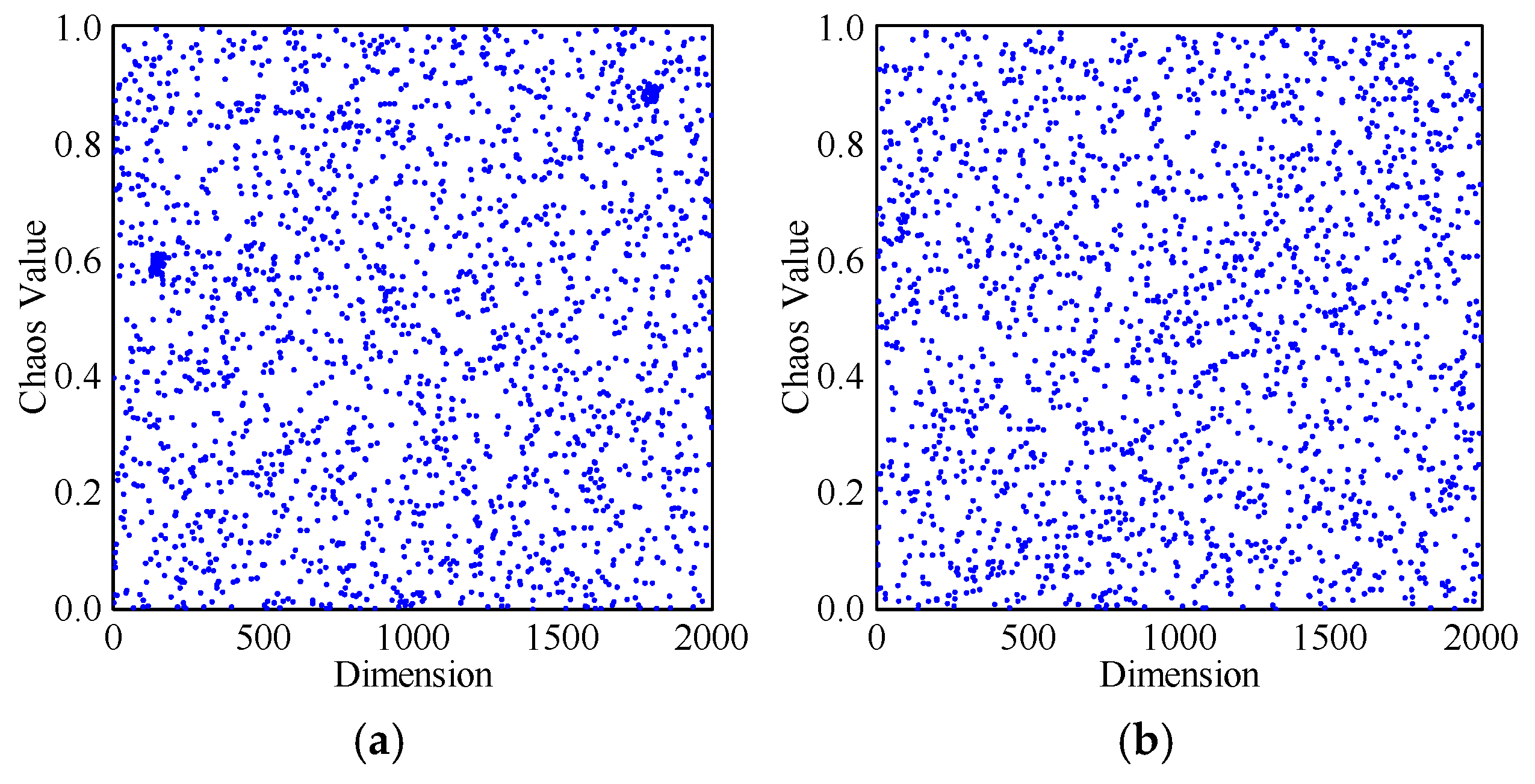
- Piecewise Linear Chaotic Map
- (2)
- Proposed Equilibrium Pool Embedding Mechanism
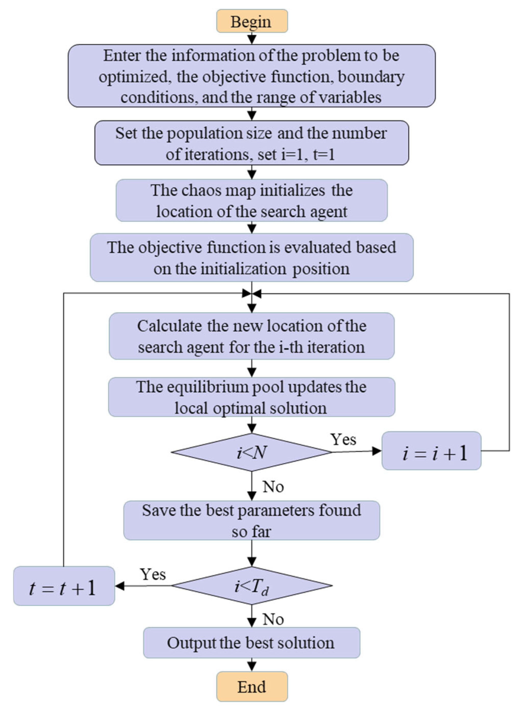
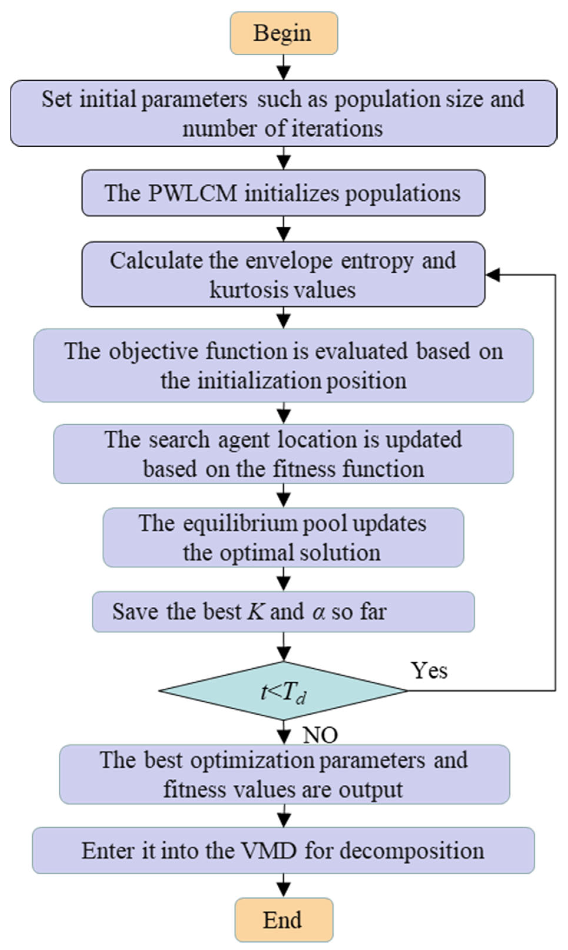
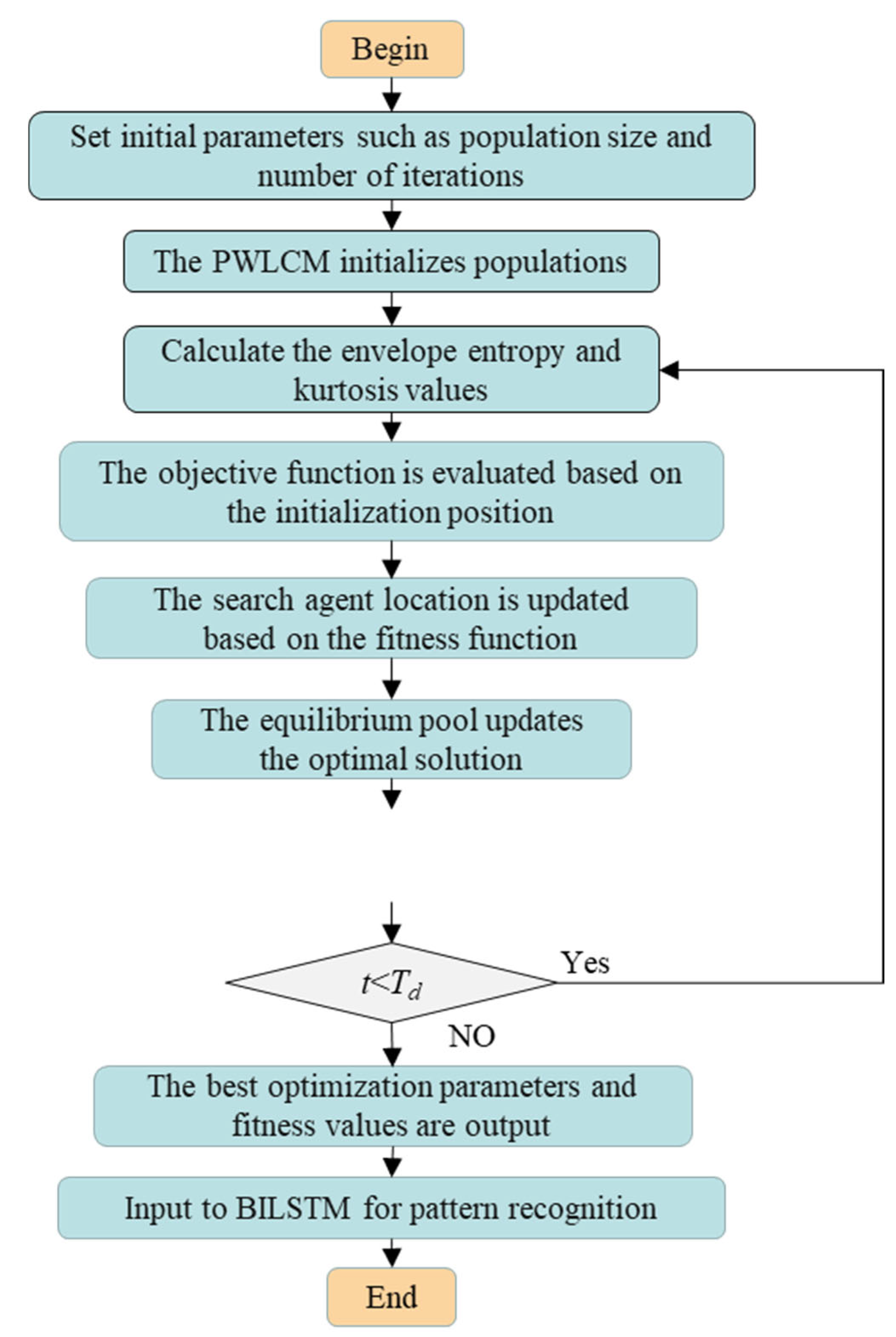
2.3. ISABO-VMD-Based Signal Denoising Method
- (1)
- Initialize ISABO parameters;
- (2)
- Replace original random initialization with a PWLCM;
- (3)
- Calculate envelope entropy and kurtosis values followed by harmonic normalization processing;
- (4)
- Evaluate objective function based on initialized positions;
- (5)
- Update search agent positions according to the fitness function;
- (6)
- Update optimal solution via equilibrium pool mechanism;
- (7)
- Store currently found optimal A and B parameters;
- (8)
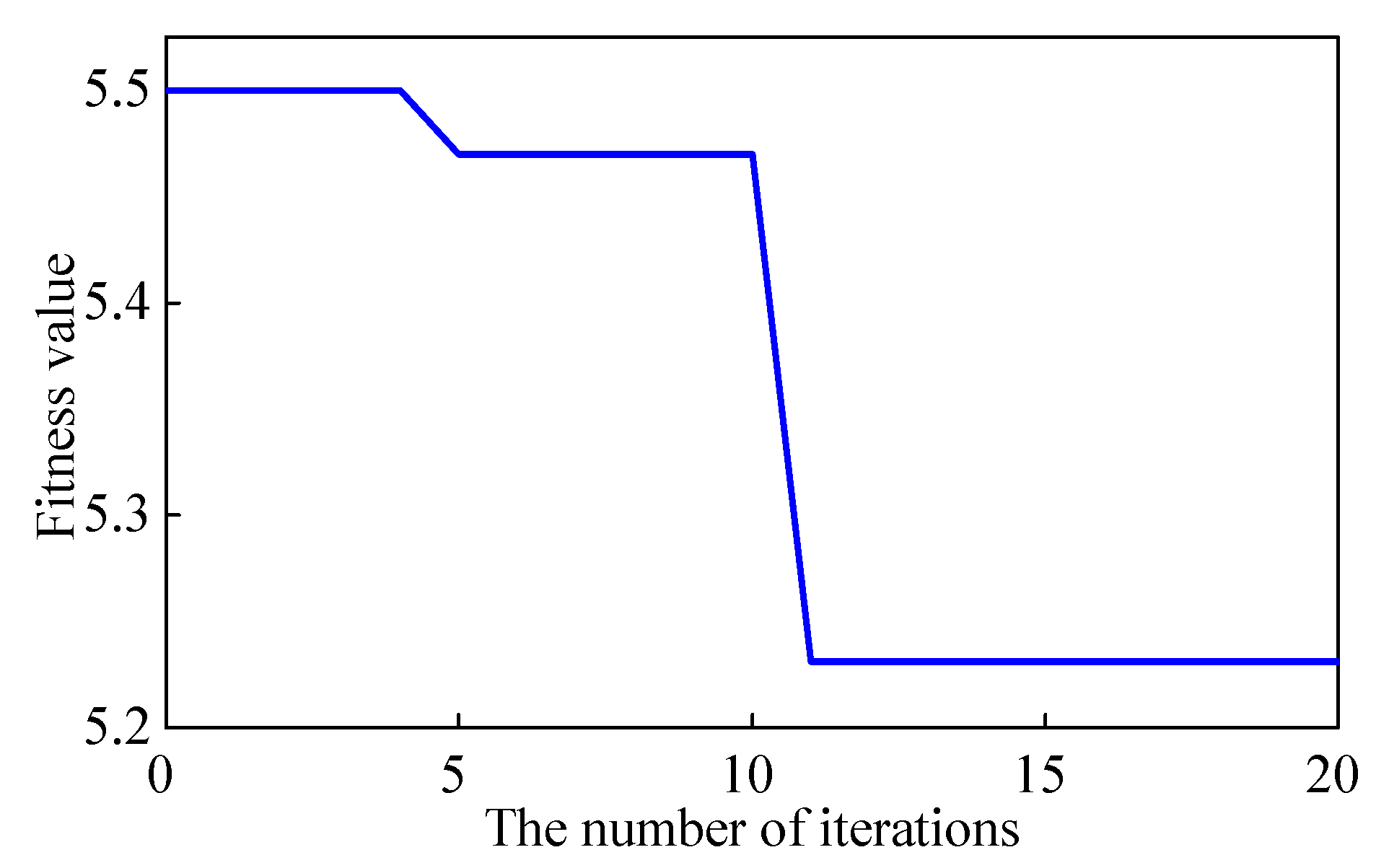
- Output optimal parameters and fitness value if maximum iterations are reached; otherwise, return to step (3).
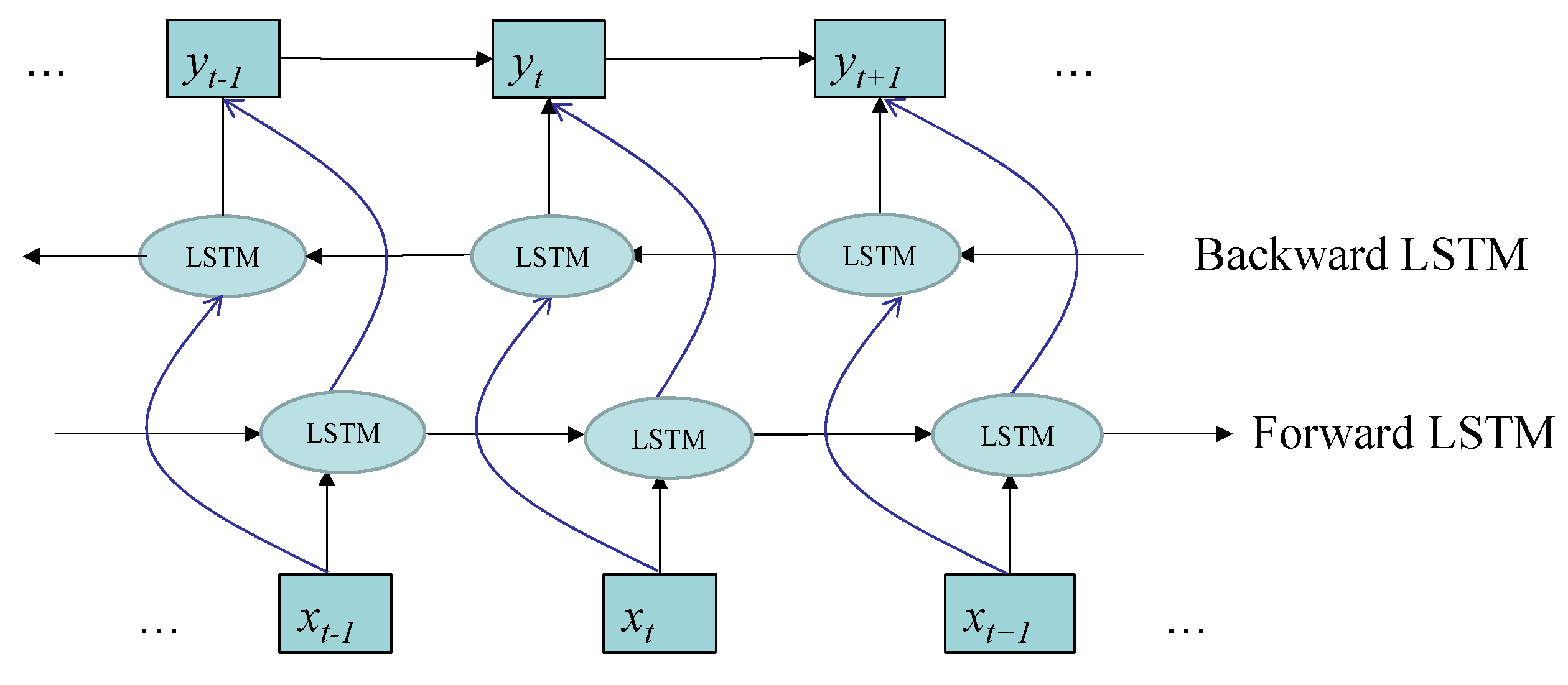
2.4. Bidirectional Long Short-Term Memory (BILSTM) Network
2.5. ISABO-BILSTM Classification Model
- (1)
- Initialize ISABO parameters: The fitness function for optimization combines envelope entropy and kurtosis into a composite evaluation metric.
- (2)
- Apply a PWLCM: Replaces the original random initialization process.
- (3)
- Calculate and normalize features: Compute both envelope entropy and kurtosis values, followed by harmonic normalization.
- (4)
- Evaluate objective function: Assessment based on initialized parameter positions.
- (5)
- Update search agents: Modify positions according to the fitness function results.
- (6)
- Optimize solution pool: Update the equilibrium pool with the current best solutions.
- (7)
- Store optimal parameters: Record the best-found values for the number of hidden layer units, the maximum training epochs, and the learning rate.
- (8)
- Termination check: If maximum iterations are reached, output optimal parameters and fitness value; otherwise, return to step (3).
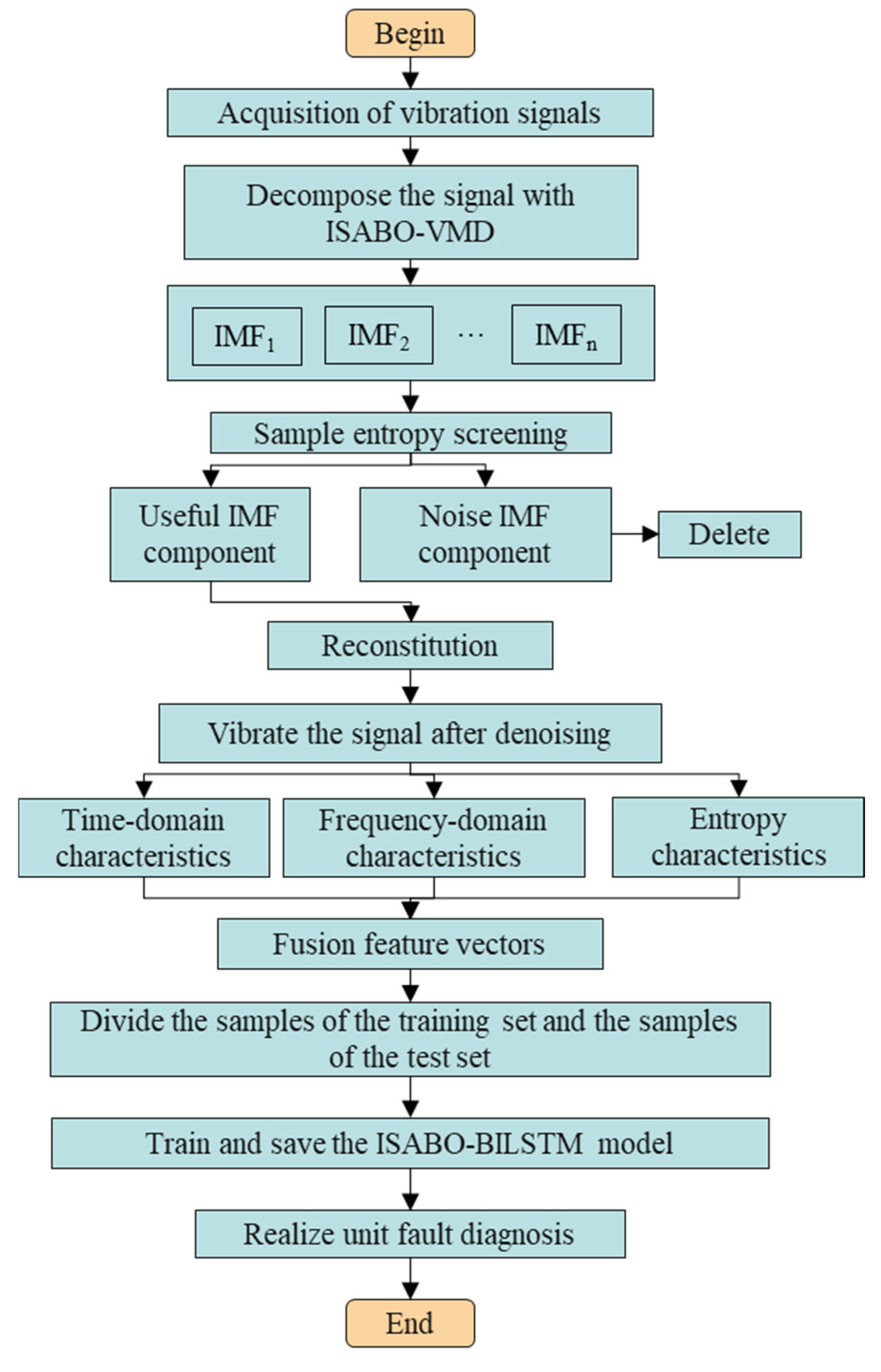
3. Adaptive VMD-BILSTM-Based Fault Diagnosis Model for Pumped Storage Units
- (1)
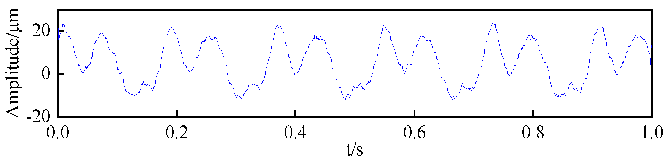
- Acquisition of vibration data from pumped storage units;
- (2)
- Decomposition of initial signals using the adaptive VMD data processing model;
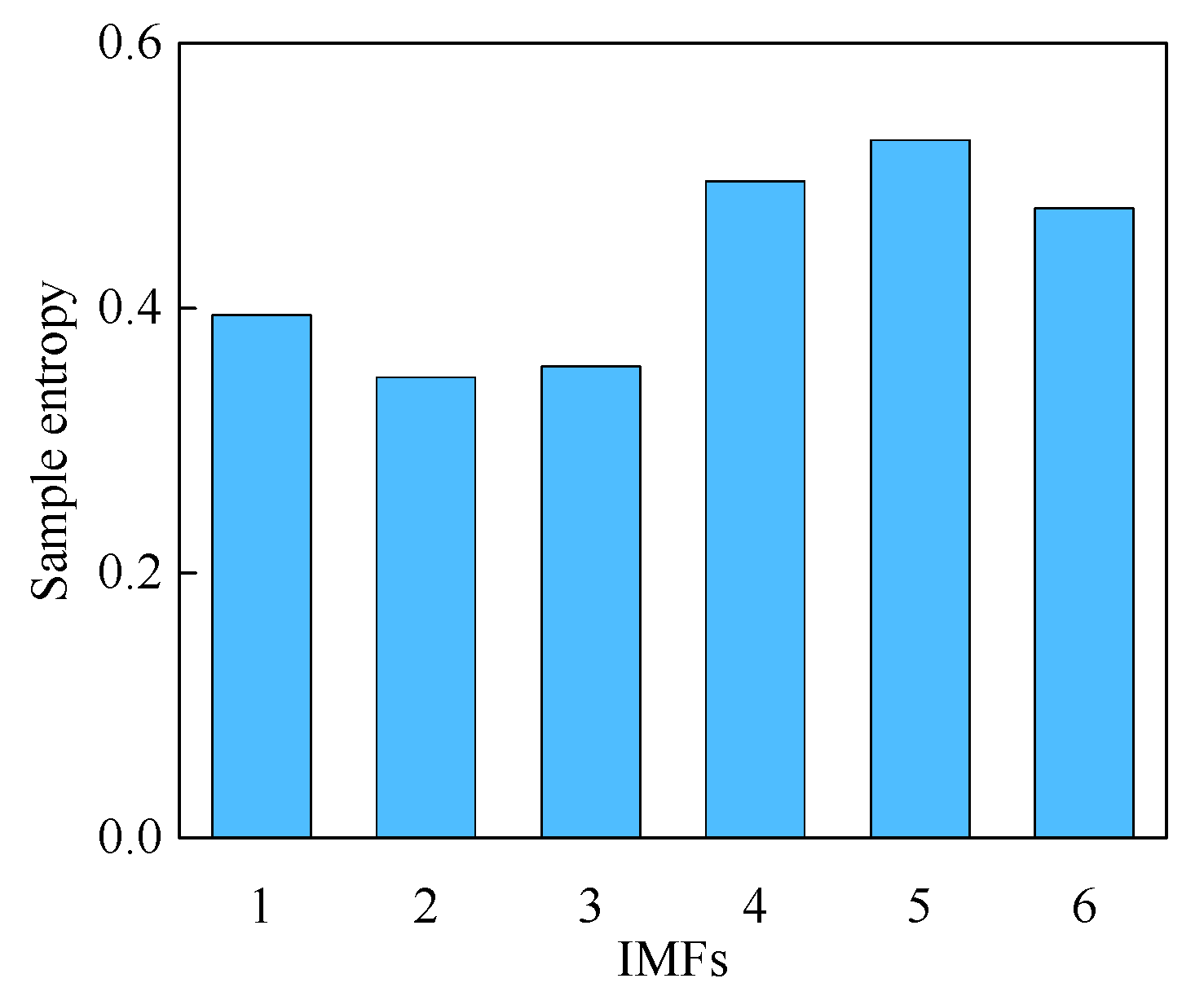
- (3)
- Calculation of sample entropy for each frequency component, with IMF components meeting composite threshold conditions being selected (optimal components are directly utilized while others are discarded as noise), followed by reconstruction of the denoised signal from the selected IMF components;
- (4)
- Computation of feature vector indicators from the denoised signal to construct the feature dataset. This study extracts a total of 26 feature vectors from vibration signals, comprising 2 entropy indicators, 14 time-domain indicators, and 10 frequency-domain indicators, to construct the feature dataset.
- (5)
- Division of feature vectors into training and testing sets according to a specified ratio;
- (6)
- Optimization of BILSTM parameters, including the number of hidden layer units (K), maximum training epochs (T), and learning rate (L);
- (7)
- Model training and subsequent fault identification for pumped storage units.
4. Case Study Analysis
4.1. Data Source
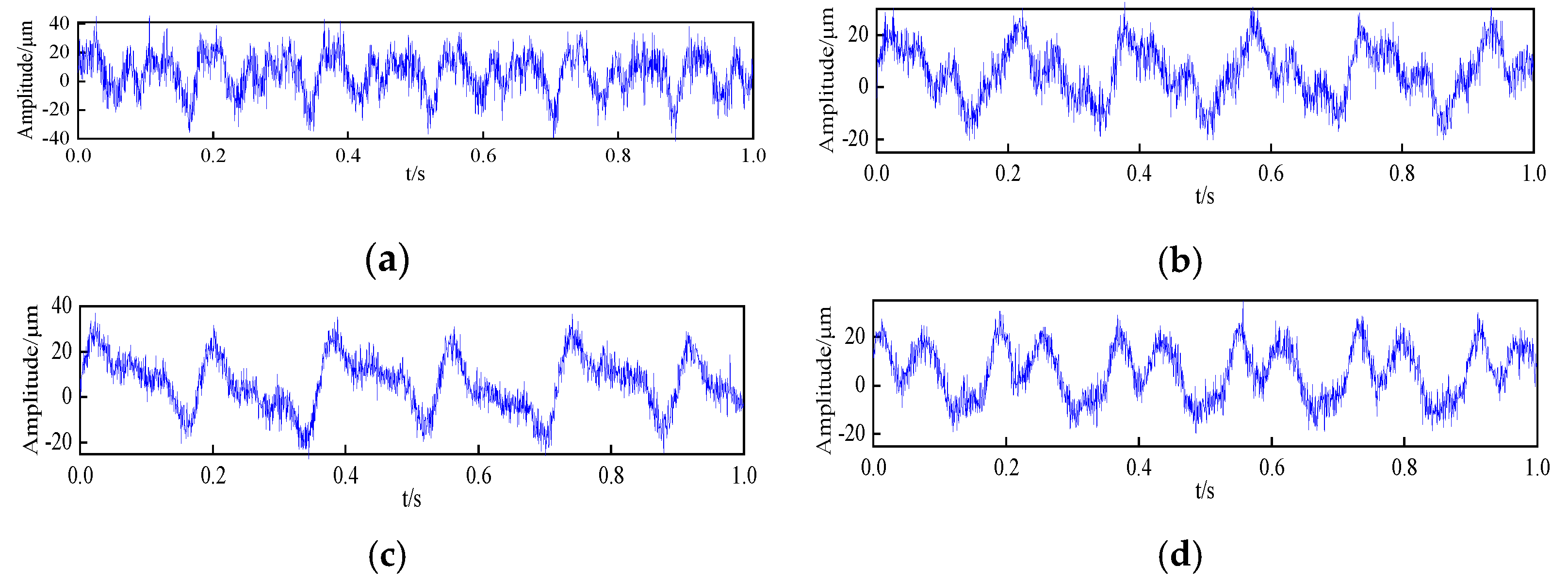
4.2. ISABO-VMD-Based Raw Signal Denoising Process
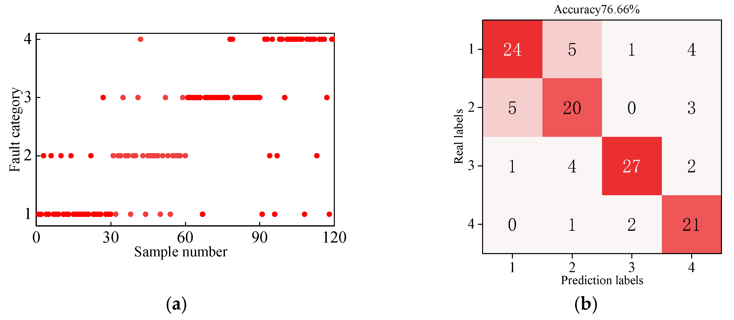
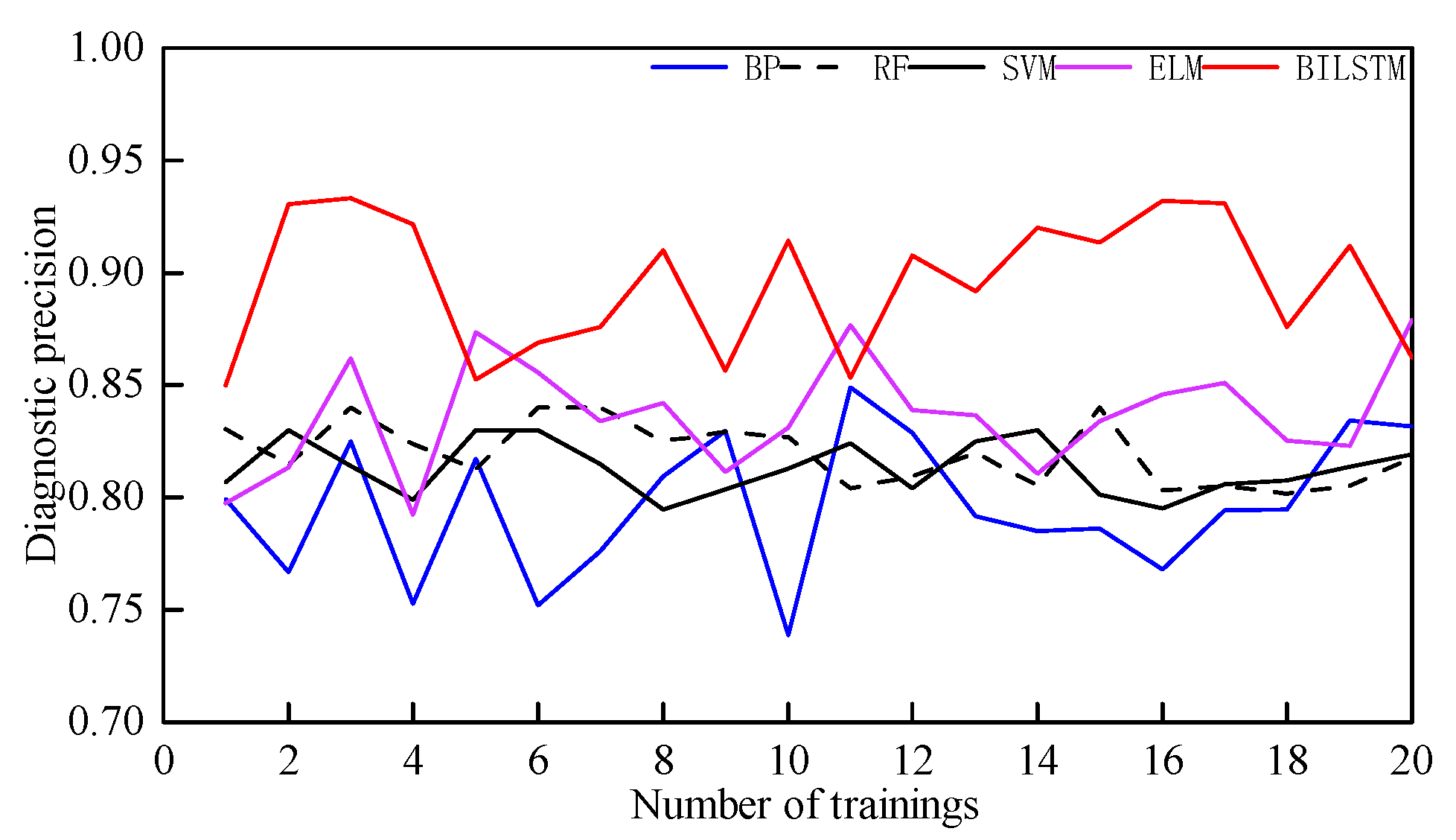
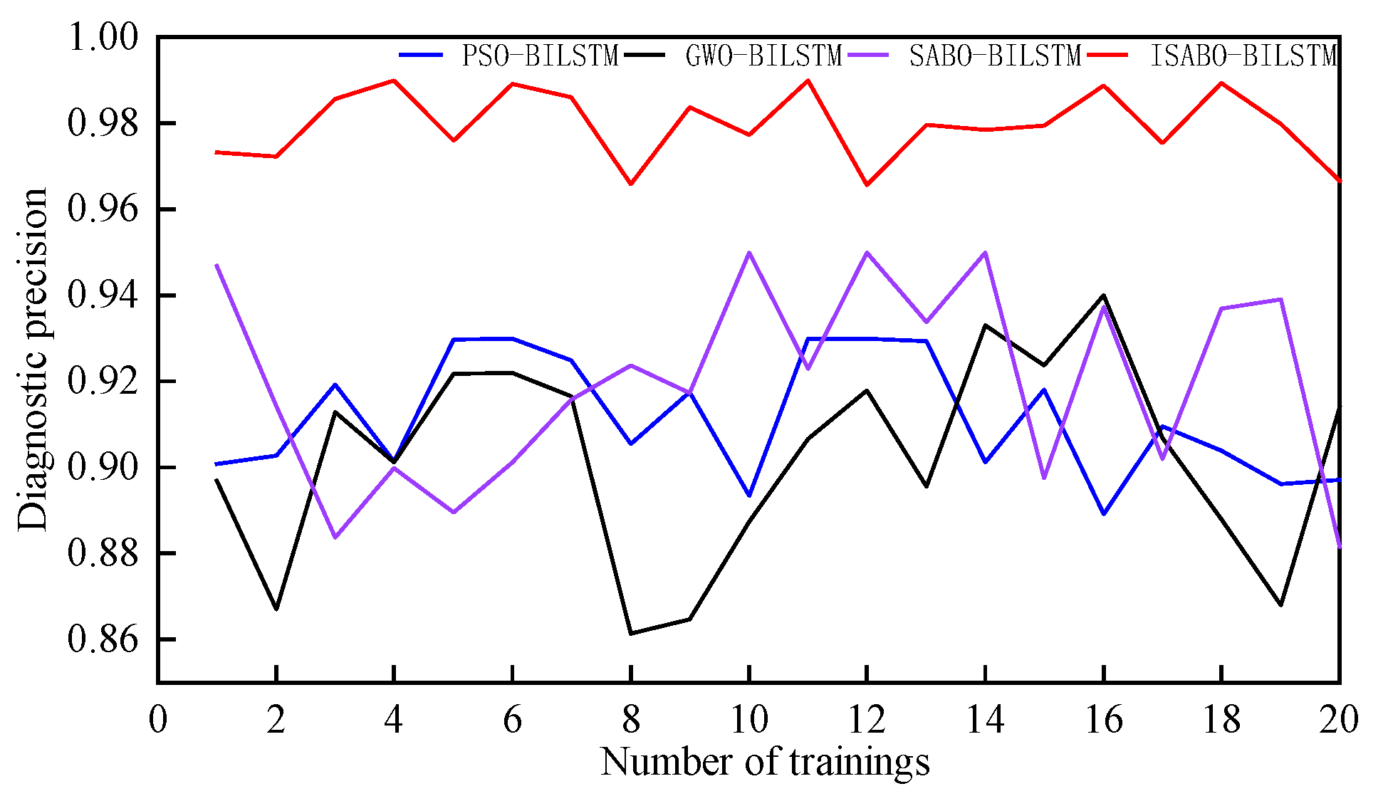
4.3. Pattern Recognition and Comparative Analysis
5. Conclusions
- (1)
- Aiming at the non-stationary and nonlinear vibration signals generated by faults in pumped storage units, an adaptive parameter optimization method for variational mode decomposition (VMD) based on the improved subtraction-average-based optimizer (ISABO) is proposed. By combining the piecewise linear chaotic map (PWLCM) with the balanced pool embedding strategy, the method achieves adaptive optimization of the VMD penalty factor and the number of decomposition layers. Experimental results demonstrate that the proposed ISABO-VMD method can effectively realize the adaptive selection of parameters.
- (2)
- To address the significant impact of key hyperparameters, such as the number of hidden units in the BILSTM network, the maximum number of training epochs, and the learning rate on diagnostic accuracy, the ISABO algorithm is introduced into the parameter optimization process. By establishing a fitness function and constraint conditions, the three key parameters are optimized in a coordinated manner, resulting in the construction of the ISABO-BILSTM intelligent diagnostic model. The experimental results indicate that, compared with traditional parameter-setting methods, the ISABO-BILSTM model demonstrates significant performance advantages, with an overall diagnostic accuracy rate reaching 97.96%.
Author Contributions
Funding
Institutional Review Board Statement
Informed Consent Statement
Data Availability Statement
Acknowledgments
Conflicts of Interest
References
- Chin, C.H.; Abdullah, S.; Ariffin, A.K.; Singh, S.S.K.; Arifin, A. A review of the wavelet transform for durability and structural health monitoring in automotive applications. Alex. Eng. J. 2024, 99, 204–216. [Google Scholar] [CrossRef]
- Lv, Y.; Wang, J.; Zhang, C.; Ding, J. Composite fault feature extraction for gears based on MCKD-EWT adaptive wavelet threshold noise reduction. Meas. Control 2025, 58, 185–195. [Google Scholar] [CrossRef]
- Yu, K.; Feng, L.; Chen, Y.; Wu, M.; Zhang, Y.; Zhu, P.; Chen, W.; Wu, Q.; Hao, J. Accurate wavelet thresholding method for ECG signals. Comput. Biol. Med. 2024, 169, 107835. [Google Scholar] [CrossRef]
- Long, S.H.; Zhou, G.Q.; Wang, H.Y. Denoising of lidar echo signal based on wavelt adaptive threshold method. Adv. Civ. Eng. 2020, 3, 215–220. [Google Scholar]
- Huang, H.R.; Li, K.; Su, W.S. An improved empirical wavelet transform method for rolling bearing fault diagnosis. Sci. China Technol. Sci. 2020, 63, 2231–2240. [Google Scholar] [CrossRef]
- Dong, J.; Zhang, Y.; Hu, J. Short-term air quality prediction based on EMD-transformer-BiLSTM. Sci. Rep. 2024, 14, 20513. [Google Scholar] [CrossRef]
- Xu, D.; Yin, J. An enhanced hybrid scheme for ship roll prediction using support vector regression and TVF-EMD. Ocean. Eng. 2024, 307, 117951. [Google Scholar] [CrossRef]
- Karbasi, M.; Ali, M.; Farooque, A.A.; Jamei, M.; Khosravi, K.; Cheema, S.J.; Yaseen, Z.M. Robust drought forecasting in Eastern Canada: Leveraging EMD-TVF and ensemble deep RVFL for SPEI index forecasting. Expert Syst. Appl. 2024, 256, 124900. [Google Scholar] [CrossRef]
- Liu, C.C.; Yang, Z.; Shi, Q. A gyroscope signal denoising method based on empirical mode decomposition and signal reconstruction. Sensors 2019, 19, 5064. [Google Scholar] [CrossRef]
- Cai, J.H.; Hu, W.W.; Wang, X.C. Fault Diagnosis ofRolling Bearing Based on EMD-ICA De-noising. J. Mach. Des. 2015, 32, 17. [Google Scholar]
- Dragomiretskiy, K.; Zosso, D. Variational mode decomposition. IEEE Trans. Signal Process. 2014, 62, 531–544. [Google Scholar] [CrossRef]
- Li, Z.; Chen, J.; Zi, Y.; Pan, J. Independence-oriented VMD to identify fault feature for wheel set bearing fault diagnosis of high speed locomotive. Mech. Syst. Signal Process. 2017, 85, 512–529. [Google Scholar] [CrossRef]
- Cui, S.; Lyu, S.; Ma, Y.; Wang, K. Improved informer PV power short-term prediction model based on weather typing and AHA-VMD-MPE. Energy 2024, 307, 132766. [Google Scholar] [CrossRef]
- Qin, C.; Huang, G.; Yu, H.; Zhang, Z.; Tao, J.; Liu, C. Adaptive VMD and multi-stage stabilized transformer-based long-distance forecasting for multiple shield machine tunneling parameters. Autom. Constr. 2024, 165, 105563. [Google Scholar] [CrossRef]
- Ding, M.; Du, B.; Wan, H.; Han, L. A signal de-noising method for a MEMS gyroscope based on improved VMD-WTD. Meas. Sci. Technol. 2021, 32, 095112. [Google Scholar] [CrossRef]
- Mao, M.; Zhou, C.; Xu, B.; Liao, D.; Yang, J.; Liu, S.; Li, Y.; Tang, T. Fault diagnosis method using MVMD signal reconstruction and MMDE-GNDO feature extraction and MPA-SVM. Front. Phys. 2024, 12, 1301035. [Google Scholar] [CrossRef]
- Huang, Y.; Lin, J.; Liu, Z. A modified scale-space guiding variational mode decomposition for high-speed railway bearing fault diagnosis. J. Sound Vib. 2019, 444, 216–234. [Google Scholar] [CrossRef]
- Zhao, Y.J.; Li, C.S.; Fu, W.L. A modified variational mode decomposition method based on envelope nesting and multi-criteria evaluation. J. Sound Vib. 2019, 468, 115099. [Google Scholar] [CrossRef]
- Jiang, W.; Zhou, J.Z.; Liu, H. A multi-step progressive fault diagnosis method for rolling element bearing based on energy entropy theory and hybrid ensemble auto-encoder. ISA Trans. 2019, 87, 235–250. [Google Scholar] [CrossRef]
- Maulik, S.; Konar, P.; Chattopadhyay, P. Fusion of vibration and current signals for improved multi class fault diagnosis of three phase induction motor. In Proceedings of the 2023 IEEE 3rd Applied Signal Processing Conference (ASPCON), Haldia, India, 24–25 November 2023; pp. 152–155. [Google Scholar]
- Cao, H.; Shao, H.; Liu, B.; Cai, B.; Cheng, J. Clustering-guided novel unsupervised domain adversarial network for partial transfer fault diagnosis of rotating machinery. IEEE Sens. J. 2022, 22, 14387–14396. [Google Scholar] [CrossRef]
- Hong, G.; Suh, D. Mel Spectrogram-based advanced deep temporal clustering model with unsupervised data for fault diagnosis. Expert Syst. Appl. 2023, 217, 119551. [Google Scholar] [CrossRef]
- Wan, L.; Zhang, G.; Li, H.; Li, C. A novel bearing fault diagnosis method using spark-based parallel ACO-K-means clustering algorithm. IEEE Access 2021, 9, 28753–28768. [Google Scholar] [CrossRef]
- Rahimilarki, R.; Gao, Z.; Jin, N.; Zhang, A. Convolutional neural network fault classification based on time-series analysis for benchmark wind turbine machine. Renew. Energy 2022, 185, 916–931. [Google Scholar] [CrossRef]
- Chen, X.; Zhang, B.; Gao, D. Bearing fault diagnosis base on multi-scale CNN and LSTM model. J. Intell. Manuf. 2021, 32, 971–987. [Google Scholar] [CrossRef]
- Shi, X.; Qiu, G.; Yin, C.; Huang, X.; Chen, K.; Cheng, Y.; Zhong, S. An improved bearing fault diagnosis scheme based on hierarchical fuzzy entropy and Alexnet network. IEEE Access 2021, 9, 61710–61720. [Google Scholar] [CrossRef]
- Zou, F.; Zhang, H.; Sang, S.; Li, X.; He, W.; Liu, X. Bearing fault diagnosis based on combined multiscale weighted entropy morphological filtering and bi-LSTM. Appl. Intell. 2021, 51, 6647–6664. [Google Scholar] [CrossRef]
- Liu, Z.; Peng, Z.; Liu, P. Multi-feature optimized VMD and fusion index for bearing fault diagnosis method. J. Mech. Sci. Technol. 2023, 37, 2807–2820. [Google Scholar] [CrossRef]
- Trojovský, P.; Dehghani, M. Subtraction-average-based optimizer: A new swarm-inspired metaheuristic algorithm for solving optimization problems. Biomimetics 2023, 8, 149. [Google Scholar] [CrossRef]


| Evaluation Indicators | Random Initialization | Chaotic Map Initialization |
|---|---|---|
| Autocorrelation Coefficient | 0.0238 | 0.0135 |
| Max-Min Ratio | 0.9426 | 0.9654 |
| Discrepancy | 0.0307 | 0.0259 |
| Name of the Parameter | Numeric Value of the Parameter |
|---|---|
| Generator output | 268 MW |
| Factor | Pump condition: 0.98, turbine condition: 0.9; |
| Rated speed | 333.3 r/min |
| Maximum rpm speed | 535.0 r/min |
| Fixed number of guide vanes | 20 |
| Number of active guide vanes | 20 |
| Rotation frequency | 50/9 Hz |
| Number of runner blades | 9 |
| Name of the Parameter | Optimal Value |
|---|---|
| Number of hidden layer elements K | 39 |
| Maximum training period T | 100 |
| Learning rate L | 0.0562 |
| Type of Failure | Average Accuracy/% | ||||
|---|---|---|---|---|---|
| BP | RF | SVM | ELM | BILSTM | |
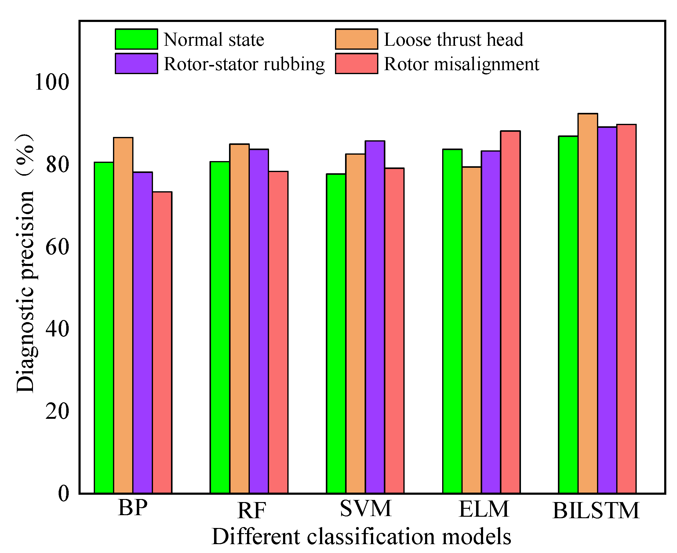
| Normal State | 80.52 | 80.77 | 77.75 | 83.77 | 86.95 |
| Loose Thrust Head | 86.56 | 84.96 | 82.58 | 79.43 | 92.39 |
| Rotor-Stator Rubbing | 78.14 | 83.78 | 85.75 | 83.34 | 89.18 |
| Rotor Misalignment | 73.38 | 78.39 | 79.14 | 88.14 | 89.75 |
| Comprehensive Accuracy | 79.65 | 81.97 | 81.31 | 83.67 | 89.56 |
| Type of Failure | Average Accuracy/% | |||
|---|---|---|---|---|
| PSO-BILSTM | GWO-BILSTM | SABO-BILSTM | ISABO-BILSTM | |
| Normal State | 88.65 | 85.07 | 86.42 | 96.29 |
| Loose Thrust Head | 89.41 | 94.18 | 94.71 | 98.60 |
| Rotor-Stator Rubbing | 92.68 | 93.70 | 95.63 | 97.34 |
| Rotor Misalignment | 93.86 | 87.98 | 91.12 | 99.59 |
| Comprehensive Accuracy | 91.15 | 90.23 | 91.97 | 97.96 |
| Classification Model | Evaluation Indicators | ||
|---|---|---|---|
| Precision/% | Recall/% | F1 Score/% | |
| PSO-BILSTM | 91.15 | 91.27 | 91.21 |
| GWO-BILSTM | 90.23 | 90.17 | 90.20 |
| SABO-BILSTM | 91.97 | 91.13 | 91.55 |
| ISABO-BILSTM | 97.96 | 97.06 | 97.51 |
Disclaimer/Publisher’s Note: The statements, opinions and data contained in all publications are solely those of the individual author(s) and contributor(s) and not of MDPI and/or the editor(s). MDPI and/or the editor(s) disclaim responsibility for any injury to people or property resulting from any ideas, methods, instructions or products referred to in the content. |
© 2025 by the authors. Licensee MDPI, Basel, Switzerland. This article is an open access article distributed under the terms and conditions of the Creative Commons Attribution (CC BY) license (https://creativecommons.org/licenses/by/4.0/).
Share and Cite
Li, H.; Li, Q.; Li, H.; Bai, L. Fault Diagnosis Method for Pumped Storage Units Based on VMD-BILSTM. Symmetry 2025, 17, 1067. https://doi.org/10.3390/sym17071067
Li H, Li Q, Li H, Bai L. Fault Diagnosis Method for Pumped Storage Units Based on VMD-BILSTM. Symmetry. 2025; 17(7):1067. https://doi.org/10.3390/sym17071067
Chicago/Turabian StyleLi, Hui, Qinglin Li, Hua Li, and Liang Bai. 2025. "Fault Diagnosis Method for Pumped Storage Units Based on VMD-BILSTM" Symmetry 17, no. 7: 1067. https://doi.org/10.3390/sym17071067
APA StyleLi, H., Li, Q., Li, H., & Bai, L. (2025). Fault Diagnosis Method for Pumped Storage Units Based on VMD-BILSTM. Symmetry, 17(7), 1067. https://doi.org/10.3390/sym17071067