Abstract
This study focuses on estimating the unknown parameters and the reliability function of the inverted-Weibull distribution, using an improved adaptive progressive Type-II censoring scheme under a competing risks model. Both classical and Bayesian estimation approaches are explored to offer a thorough analysis. Under the classical approach, maximum likelihood estimators are obtained for the unknown parameters and the reliability function. Approximate confidence intervals are also constructed to assess the uncertainty in the estimates. From a Bayesian standpoint, symmetric Bayes estimates and highest posterior density credible intervals are computed using Markov Chain Monte Carlo sampling, assuming a symmetric squared error loss function. An extensive simulation study is carried out to assess how well the proposed methods perform under different experimental conditions, showing promising accuracy. To demonstrate the practical use of these methods, a real dataset is analyzed, consisting of the survival times of male mice aged 35 to 42 days after being exposed to 300 roentgens of X-ray radiation. The analysis demonstrated that the inverted Weibull distribution is well-suited for modeling the given dataset. Furthermore, the Bayesian estimation method, considering both point estimates and interval estimates, was found to be more effective than the classical approach in estimating the model parameters as well as the reliability function.
1. Introduction
Advancements in technology and manufacturing have resulted in the development of highly reliable modern products that often exhibit much longer lifespans before failure. As a result, traditional life testing methods, which rely on observing failures within a reasonable time period, have become less effective. This challenge emphasizes the need for more advanced statistical tools that can efficiently analyze lifetime data under time constraints. In such cases, researchers often use censoring schemes as an effective way to collect sufficient data without waiting for all test units to fail. The literature outlines several censoring schemes, including Type-I and Type-II censoring. In Type-I censoring, the test ends after a predetermined time, while in Type-II censoring, the test concludes once a specified number of failures have occurred. A more flexible alternative is the progressive Type-II censoring (PTIIC) scheme, which allows for the removal of surviving units at multiple stages during the experiment. For more information on the application of PTIIC, one may refer to Balakrishnan et al. [1], Balakrishnan and Hossain [2], Wu and Gui [3], and Dey et al. [4], among others.
Ng et al. [5] proposed a more flexible censoring scheme known as the adaptive progressive Type-II censoring (APTIIC) plan. This approach not only encompasses the traditional PTIIC plan as a specific case but also enhances the efficiency of statistical inference compared to the censoring plan introduced by Kundu and Joarder [6]. The APTIIC scheme has been widely applied in many studies, such as Sobhi and Soliman [7], Kohansal and Shoaee [8], Panahi and Asadi [9], Haj Ahmad et al. [10], Vardani et al. [11], and Yu et al. [12]. However, Ng et al. [5] noted that the APTIIC scheme is effective for statistical inference only when testing time is not a concern. For highly reliable units, it can lead to excessively long testing durations, making it unsuitable for ensuring reasonable test lengths. To address this, Yan et al. [13] introduced the improved APTIIC (IAPTIIC) plan. The IAPTIIC plan generalizes several existing censoring methods, including PTIIC and APTIIC schemes, among others. Additionally, it guarantees that experiments are completed within a predefined time frame, effectively addressing the challenges posed by prolonged testing durations. This advancement makes the IAPTIIC scheme a valuable tool for conducting reliability studies under time-constrained conditions. For more details on recent studies concerning the IAPTIIC strategy, see Dutta and Kayal [14], Nassar and Elshahhat [15], Dutta et al. [16], Zhang and Yan [17], and Irfan et al. [18]. The next section offers a detailed description of the IAPTIIC scheme.
In various medical and engineering studies, the failure of test units is frequently influenced by multiple risk factors or causes. These factors, which can be conceptualized as competing influences, contribute to the eventual breakdown of the unit. For instance, in medical research, a patient’s health outcome may be impacted by competing risks such as disease progression, treatment side effects, or unrelated health complications. Because these risk factors operate simultaneously and each possesses the potential to induce failure, they are considered to be in competition with one another. This phenomenon is formally recognized in the statistical literature as the competing risks model. See Crowder [19] for more competing risks examples. When analyzing competing risks data, researchers frequently focus on assessing the impact of a specific risk while considering the influence of other contributing factors. Ideally, the data set for such analysis includes the lifetime of the failed unit along with an indicator variable that specifies the cause of failure. The causes of failure can be modeled as either independent or dependent events. In this study, we adopt the latent failure time model proposed by Cox [20]. Within this framework, the competing causes of failure are assumed to follow independent distributions. The competing risks model has been widely studied due to its significant importance in fields such as survival analysis, reliability engineering, and medical research see for example, the works of Kundu et al. [21], Sarhan [22], Zhang [23], Fan et al. [24], Ren and Gui [25], and Tian et al. [26].
Elshahhat and Nassar [27] investigated the Weibull competing risks model using the IAPTIIC scheme. Their work focused on both classical and Bayesian estimation methods for the model parameters and the reliability (RF). They used the Weibull distribution due to its widespread applications. It is widely applied in reliability engineering to model time-to-failure of mechanical systems like turbines, in survival analysis for patient survival times in medical studies, in meteorology for wind speed distributions, in material science for characterizing material strength, in hydrology for extreme events like floods, and in quality control for assessing product lifetimes. While the competing risks model and the IAPTIIC scheme are highly significant, no studies have yet explored this framework for other lifetime distributions, despite the limitations of the Weibull distribution in modeling data with non-monotonic and unimodal hazard rate functions. To address this gap, this study employs the flexibility of the inverted-Weibull (IW) distribution to analyze reliability within the competing risks framework using IAPTIIC data. The IW distribution is chosen for its ability to accommodate non-monotonic hazard rates and provide a more accurate fit to empirical data; see Keller and Kanath [28]. Its versatility makes it particularly suitable for modeling diverse data types across various fields. Notable practical applications of the IW distribution include modeling the time to breakdown of insulating fluids, the degradation of mechanical components, survival and reliability data, and in extreme value analysis for modeling maximum or minimum values such as stock price fluctuations. See for more details about the IW distribution, AL-Essa et al. [29], Jana and Bera [30], and Mou et al. [31]. Under the competing risks model, several researchers have explored estimation problems for the IW distribution under different sampling schemes. For instance, El Azm et al. [32] investigated parameter estimation under APTIIC sampling. Samia et al. [33] focused on making statistical inferences using a generalized progressive hybrid Type-I censoring scheme. Additionally, Alotaibi et al. [34] examined parameter estimation by applying the expectation–maximization algorithm in the case of complete sample.
It is evident that the available studies have primarily focused on estimating the parameters of the IW competing risks model using traditional sampling plans or complete data. None of these works have explored more advanced censoring schemes such as the IAPTIIC scheme. Furthermore, while parameter estimation has been widely addressed, the estimation of the RF has generally been overlooked. Considering the advantages of the IAPTIIC scheme over conventional censoring methods, and the flexibility of the IW competing risks model in handling data with multiple failure causes, this study aims to investigate both classical and Bayesian estimation methodologies for the unknown parameters and the RF under IAPTIIC competing risks data.The estimation methods involve obtaining both point estimates and interval estimates. By integrating classical and Bayesian methodologies, this study provides a useful framework for reliability analysis in the presence of competing risks which may be of interest for practitioners in fields such as engineering, medicine, and reliability testing. The main contributions of this study can be presented as follows:
- Derivation of maximum likelihood estimates (MLEs) and construction of approximate confidence intervals (ACIs) for the unknown parameters and RF of the IW competing risks model under the IAPTIIC scheme.
- Development of Bayesian estimation procedures using Markov Chain Monte Carlo (MCMC) methods to obtain Bayes point estimates and highest posterior density (HPD) credible intervals.
- Comprehensive simulation study conducted to evaluate the performance and accuracy of both classical and Bayesian estimation methods under various experimental scenarios.
- Application of the proposed methods to real-world competing risk data set to demonstrate their practical utility and effectiveness in estimating model parameters and RF.
The remainder of this study is structured as follows: Section 2 discusses the IW distribution and the IAPTIIC scheme under the competing risks model. Section 3 derives the MLEs and constructs the ACIs for the IW parameters and the RF. Section 4 focuses on Bayesian estimation, employing the squared error (SE) loss function to estimate the parameters and the related RF. Section 5 presents the simulation study design and discusses the corresponding results, evaluating the performance of the proposed methods. Section 6 demonstrates the practical application of the methodologies by analyzing real-world data sets within the competing risks framework. Finally, Section 7 concludes this study, summarizing the key findings and their implications for reliability analysis and related fields.
2. Model Description
Suppose n identical items are put on a life test, and their lifetimes are represented by independent and identically distributed (i.i.d.) random variables, denoted as . For simplicity and without loss of generality, we assume that there are only two competing risks influencing the failure of these units. Under this assumption, the failure of each unit can be attributed to one of these two competing causes. Then, we have
where , for , represents the latent failure time of the i-th testing unit under the j-th cause of failure. Additionally, it is assumed that the latent failure times and , for , are independent. When a failure occurs, the researcher records the failure time and identifies the specific cause of failure, denoted by the indicator variable , with , where if the i-th failure is attributed to the first cause, and if it is due to the second cause. This indicator variable helps identify the specific risk factor responsible for each observed failure. Assume that , follows the IW distribution with scale parameter and shape parameter , and it will be referred to as . Then, the associated probability density function (PDF) and distribution function, can be written, respectively, as
and
Let and . Then, the RF at a distinct time t, defined as , , can be expresses as follows
where .
The process of generating an IAPTIIC sample in the presence of competing risks can be described as follows: Let represent the predefined number of failures to be observed, and let denote the predetermined removal pattern established before the experiment begins. Additionally, the researcher sets two threshold times, and , where and . These thresholds define the experimental time constraints: the experiment is allowed to continue beyond but must not exceed . This setup ensures that the experiment remains within a controlled time frame while accommodating the adaptive nature of the censoring scheme. When the i-th unit fails, with failure time represented by for , the researcher randomly removes units from the remaining surviving items. The cause of failure is recorded at each failure event. This procedure continues until the test concludes based on one of the following three scenarios:
- Case I: If , the researcher terminates the test at and discards all the remaining surviving items. This results in the conventional PTIIC sample.
- Case II: If , where represents the number of failures occurring before time and , we set . The experiment is terminated at the time of the m-th failure, and all remaining units are removed at that time. Note that this scenario corresponds to the well-known APTIIC sample.
- Case III: If , the experiment is terminated at . In this scenario, no items are removed once the test time exceeds the first threshold . Here, represents the number of failures observed before time . At , all remaining units are removed, i.e., .
In this case, the observed IAPTIIC competing risks data will be
where for the sake of simplicity. Let Q refers to the total number of observed failures and denote an indicator function for the event . Using this, we define
From this, it follows that , for , represents the number of observed failures associated with cause k, where . Let be an IAPTIIC competing risks sample drawn from a continuous population. Then, the joint likelihood function of the observed data, can be expressed as follows
where the available options for Q, D, , and are provided in Table 1.

Table 1.
Various options for for Q, D, , and .
3. Maximum Likelihood Estimation
In this part, we derive the MLEs and the associated ACIs for the model parameters and , ). Additionally, we obtain the MLE and ACI for the RF. These derivations are conducted under the framework of IAPTIIC competing risks data and based on the above-mentioned assumptions.
3.1. MLEs and ACIs for the Model Parameters
Consider an observed IAPTIIC competing risks sample , drawn from an IW population with a PDF and distribution function given by (1) and (2), respectively. Using these, the likelihood function can be expressed based on (4) as follows
where and . The log-likelihood function corresponding to (Lik1) is
By equating the first-order partial derivatives of (6) with respect to and to zero, we obtain a system of four normal equations. These equations must be solved simultaneously to acquire the MLEs of the model parameters, denoted as and . The normal equations to be solved are as follows
and
where and .
From Equations (7)–(10), it is evident that the classical estimators cannot be expressed in closed-form solutions. As a result, obtaining the MLEs requires the use of a numerical iterative approach. One such method is the Newton–Raphson algorithm, which can be employed to solve the system of normal equations and compute the MLEs and for .
To construct interval estimates for model parameters and , it is necessary to obtain the asymptotic variance–covariance matrix. This matrix is typically derived from the Fisher information matrix. However, due to the complexity of obtaining the exact closed-form expression of the Fisher information matrix, we instead utilize the observed Fisher information matrix as an approximation. This approach allows us to estimate the required variances and covariances. The estimated variance-covariance matrix can be expressed as follows
where is the MLE of , and
and
where , and , with .
By utilizing the asymptotic normality property of the MLEs, we can express the distribution of as , where is the estimated variance–covariance matrix, as provided in (12). Using this asymptotic distribution, we can construct ACIs for the unknown parameters and , where as
where is the critical value from the standard normal distribution corresponding to the significance level , and is the estimated variances, obtained from the diagonal elements of . It is important to mention here that this method relies on the large-sample properties of MLEs, ensuring that the intervals are asymptotically valid and provide reliable estimates of the parameter uncertainty. However, for small sample sizes, the accuracy of these intervals may be limited, and alternative methods such as Bayes credible could be considered for improved performance.
3.2. MLE and ACI for the RF
Using the invariance property of the MLEs, the MLE of the RF at a distinct time t, denoted as , can be obtained by substituting the MLEs of the parameters and , where into the expression for the RF presented in (3). This property ensures that the MLE of the RF retains the same properties as the MLEs of the parameters. Thus, the MLE of the RF can be obtained using (3) as
On the other hand, to construct the associated ACIs for , we first approximate the variance of using the delta method. The delta method utilizes the asymptotic normality of the MLEs and provides an approximation of the variance of a function of the parameters. Specifically, the variance of is approximated as
where
and
Once the approximate variance of is obtained, the ACI for can be computed as follows
4. Bayesian Estimation
In this section, we explore the Bayesian estimation approach to derive the Bayesian estimators and HPD credible intervals for the model parameters and the related RF. The Bayes estimates and the interval ranges are obtained using the MCMC technique through sampling from the posterior distribution. The Bayes point estimates are computed under the SE loss function, a commonly used symmetric loss function in Bayesian inference. In Bayesian analysis, the process begins by specifying prior distributions for the parameters. From the likelihood function given in (5), it is clear that conjugate priors are not available for and , . To overcome this limitation, we adopt gamma priors for these parameters. Gamma priors are particularly advantageous as they allow flexibility in adjusting the range of the unknown parameters while maintaining computational simplicity. These priors are versatile and can effectively incorporate various forms of prior knowledge. Moreover, the use of gamma priors does not complicate posterior evaluation or computational procedures, especially when employing MCMC methods.
Let and where for are the hyper-parameters and are assumed to be known. The joint prior distribution of and , is then expressed as follows:
By combining the likelihood function in (5) with the joint prior distribution in (13), the joint posterior distribution of the model parameters can be derived as follows:
where
Let represent a parametric function of the unknown parameters . The Bayes estimator of is typically obtained under a chosen loss function, and one of the most commonly used loss functions is the SE loss function. The SE loss function is commonly used due to its mathematical tractability and desirable properties, such as minimizing the mean squared error. However, it is important to note that the Bayes estimator can be easily obtained under other loss functions as well. Under the SE loss function, the Bayes estimator of , denoted as , can be expressed as the expected value of with respect to the posterior distribution of the parameters . Specifically, it is given by
where represents the posterior expectation based on the observed data. Based on the posterior distribution in (14), the Bayes estimator in (15), can be obtained as
The Bayes estimator in (16) requires computing a very complex integrals, which is analytically intractable due to the complicated posterior distribution. While numerical methods like Monte Carlo integration can approximate these integrals, they are often computationally expensive, especially with many parameters or complex posteriors as in our case. To address this, we use the MCMC method, which allows direct sampling from the posterior distribution in (14). These samples are then used to approximate Bayes estimates and construct the HPD credible intervals. A key step in implementing the MCMC method is deriving the full conditional distributions of the unknown parameters. Using the joint posterior distribution provided in (14), we can express the conditional distributions for the parameters and , as
and
Upon initial inspection, the full conditional distributions presented in (17)–(20) do not align with any standard or widely recognized probability distributions. Consequently, traditional sampling techniques, such as inverse transform sampling, are not applicable to generate random samples from these distributions. To address this limitation, we employ the Metropolis–Hastings (M–H) algorithm, a well-known MCMC method. The M–H algorithm is particularly effective for sampling from complex or non-standard distributions, as it utilizes a candidate-generating distribution, referred to as the proposal distribution, to yield potential samples. In this study, we utilize the normal distribution as the proposal distribution for all parameters. The mean and variance of this normal distribution are determined based on the MLEs of the parameters. The M–H algorithm operates by iteratively proposing new samples from the proposal distribution and accepting or rejecting these samples based on an acceptance probability that guarantees the resulting Markov chain converges to the target posterior distribution. The procedure for generating random samples using the M–H algorithm involves the following steps:
- 1.
- Initialize the algorithm by setting the starting values as , where and are the MLEs of the parameters and .
- 2.
- Set the iteration counter .
- 3.
- Use the conditional distribution given in (17) to generate as follows:
- •
- Generate a candidate value from a normal distribution .
- •
- Compute the acceptance probability (AP):
- •
- Draw a random number u from a uniform distribution .
- •
- If , accept and set . Otherwise, retain the previous value .
- 4.
- Repeat step 3 to generate the following:
- 5.
- Using the updated values , compute the RF at iteration j, denoted by , as follows:
- 6.
- Increment the iteration counter by setting .
- 7.
- After repeating steps 3 through 6 multiple times, discard an initial set of iterations as the burn-in period to ensure the Markov chain has converged to its stationary distribution. The remaining iterations yield the following sequences:where represents the number of iterations retained after discarding the burn-in period.
Once the MCMC samples have been generated, they can be readily utilized to compute the Bayes estimates and the HPD credible intervals for the model parameters and the RF. Under the SE loss function, the Bayes estimates are obtained as the posterior means of the respective parameters. Specifically, the Bayes estimates for the parameters , , and the RF are calculated as
Additionally, the HPD credible intervals provide the shortest possible interval for a given probability level under the posterior distribution. To illustrate the computation process, we outline the steps to calculate the HPD credible interval for the RF below. The same procedure can be applied analogously to other parameters using the MCMC-generated samples.
- 1.
- Sorting the MCMC samples as .
- 2.
- Identify the index within the range that satisfies the following condition:
- 3.
- The HPD credible interval for the RF is then given by
5. Monte Carlo Comparisons
To show how the efficiency of the theoretical acquired findings on , , and behave, obtained through maximum likelihood and Bayesian methodologies, we implement various Monte Carlo comparisons on the IW lifespan model from IAPTIIC competing risks.
5.1. Simulation Design
By assigning and , by varying key experimental factors, such as the total number of test units (n), the effective sample size (m), the removal scheme (), and the threshold points (), we generate 1000 IAPTIIC competing risks from an IW distribution. Using , the corresponding plausible value of is taken as 0.9328. Specifically, for each unknown quantity, we evaluate it using six simulation setups; see Table 2. In this table, (for example) means that 5 is repeated 2 times, and FP% refers to the failure percentage given by .
Table 2.
Different Monte Carlo simulation setups.
To gather an IAPTIIC competing risks data from an IW distribution, conduct the following:
- Step 1.
- Assign parameter values for and .
- Step 2.
- Generate a PTIIC competing risks sample as:
- a.
- Collect independent observations of size m from a uniform distribution, say .
- b.
- Compute
- c.
- Define for .
- d.
- Set
- Step 3.
- Identify at threshold time and discard observations
- Step 4.
- Generate order statistics for observations from a truncated distribution.
- Step 5.
- Assign failure causes based on indicators .
- Step 6.
- Compile an IAPTIIC competing risks sample as depicted in Table 1.
For each simulated IAPTIIC data set, the MLEs and 95% ACIs at a significance level of are computed. The Newton–Raphson method, implemented via the ‘maxLik’ package (by Henningsen and Toomet [35]) in R, is employed to estimate the unknown parameters and .
Bayesian estimation incorporates two informative prior sets of , namely
- Prior-1: , , and ;
- Prior-2: , , and .
These priors are selected such that their mean values align with the expected parameter values. In cases where prior knowledge is unavailable, frequentist estimates are preferred due to computational efficiency. Bayesian estimates are obtained using the MCMC sampler discussed in Section 4, generating 12,000 MCMC samples and discarding the first 2000 as burn-in. The posterior summaries are computed from the remaining 10,000 samples using the ‘coda’ package introduced by Plummer et al. [36].
Bayesian inference inherently depends on prior beliefs. A sensitivity study assesses how posterior estimates respond to different plausible choices of priors. This is especially important when prior information is uncertain or partially subjective; one needs to justify the reliability of conclusions, or regulatory or scientific standards demand robustness checks. For this purpose, to evaluate the robustness and credibility of posterior inference, a sensitivity study is performed using four distinct types of priors, namely informative, noninformative (improper), weak, and overdispersed. Figure 1 illustrates the sensitivity of posterior estimates for parameters , , , and to four predefined prior types. It reveals that the informative priors yield the most concentrated (least variable) posterior distributions, while improper and overdispersed priors result in wider spreads, indicating higher uncertainty. This demonstrates that stronger prior beliefs tighten inference, whereas vague or extreme priors allow the data more influence but introduce greater variability. So, the posterior estimates through gamma priors support the robustness and credibility of Bayesian computations.
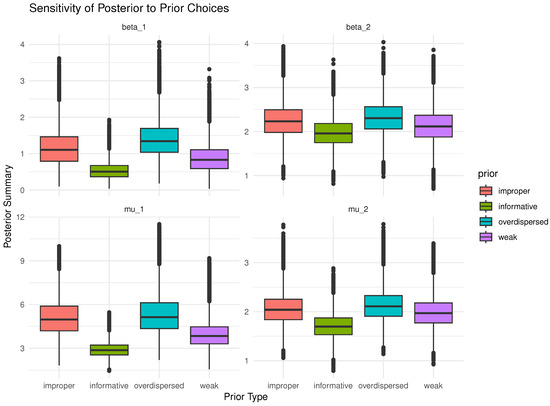
Figure 1.
Sensitivity of posterior estimates to several prior distributions of and for .
The mean point estimate (MPE) of , , or (say, ) (for instance) is obtained as
where represents the estimate of obtained at jth sample.
Point estimators are evaluated based on their root mean squared errors (RMSEs) and mean relative absolute biases (MRABs), defined as
and
respectively.
Interval estimators are assessed based on their average interval lengths (AILs) and coverage probabilities (CPs), respectively, as
and
where is the indicator, and (,) denotes the estimated interval bounds.
5.2. Simulation Results and Discussions
All simulation outcomes of , , and are listed in Table A1, Table A2, Table A3, Table A4, Table A5, Table A6, Table A7, Table A8, Table A9 and Table A10. Specifically, Table A1, Table A2, Table A3, Table A4 and Table A5 summarize the MPEs, RMSEs, and MRABs in the first, second, and third columns, respectively, while AILs and CPs for 95% ACI/HPD intervals are detailed in the first and second columns, respectively, in Table A6, Table A7, Table A8, Table A9 and Table A10. For brevity and to enhance readability, while maintaining focus on the narrative flow, all simulation tables are moved to Appendix A.
From Table A1, Table A2, Table A3, Table A4, Table A5, Table A6, Table A7, Table A8, Table A9 and Table A10, in terms of the lowest RMSE, MRAB, and AIL values as well as the highest CP values, we list the following assessments:
- The estimation outcomes for all unknown parameters, specifically and for , as well as the reliability function , demonstrate robust performance across a wide range of simulated scenarios, reflecting the stability and consistency of the proposed inferential methods.
- An increase in the sample size n or FP% leads to improved estimation precision for all parameters, including , , and . A comparable enhancement in estimation accuracy is also observed when the total number of removals, , is reduced.
- The integration of informative gamma prior distributions within the Bayesian framework yields MCMC-based point and 95% HPD interval estimates for , , and that surpass the frequentist point and 95% ACIs in terms of accuracy and interval efficiency.
- Among the Bayesian approaches considered, estimates derived from Prior-2 exhibit superior performance relative to those based on Prior-1. This advantage is attributed to the reduced posterior variance under Prior-2, which translates into more precise inference.
- Comparing the progressive removal designs (presented in Table 2), reveals that:
- –
- The estimates of behave better based on removal designs used in [1] (when FP% = 50%) and [4] (when FP% = 75%) than others;
- –
- The estimates of behave better based on removal designs used in [3] (when FP% = 50%) and [6] (when FP% = 75%) than others;
- –
- The estimates of behave better based on removal designs used in [2] (when FP% = 50%) and [3] (when FP% = 75%) than others.
- Increasing the thresholds provide the following trends:
- –
- The RMSEs, MRABs, and AILs of and decrease, whereas those of increase.
- –
- The CPs of increase, while the CPs of decrease.
- Across most simulation configurations, the CPs of both ACIs and HPD intervals for (), , and closely approximate the nominal 95% level, indicating reliable interval estimation performance.
- As a recommendation, considering the two competing risk scenarios analyzed using the proposed IAPTIIC framework, we advocate for Bayesian estimation techniques when evaluating the parameters or reliability index of the IW model.
6. Radiobiology Application
Radiation exposure in biological organisms is crucial for understanding its effects on cellular function, genetic stability, and overall health. In radiobiology, toxicology, and medical science, it has been used frequently to explore radiation exposure risks and therapeutic interventions. This application captures the effects of 300 roentgens of radiation on male mice aged 35 to 42 days (5–6 weeks) in a controlled laboratory setting. Its precise measurements and experimental design make it a valuable resource for understanding radiation-induced biological changes; for additional details, see Kundu et al. [21], Alotaibi et al. [37], Alotaibi et al. [38], among others.
In Table 3, the radiation data set (consisting of 77 lifetimes) is distinguished as 0 (lifetime is censoring), 1 (death of life is caused by reticulum cell sarcoma), or 2 (death of life caused by otherwise). Ignoring lifetimes of male mice still alive, in this application, we only examine observations of radiation dose from causes 1 and 2. For computational requirements, each original has been divided by a hundred.
Table 3.
Radiation dose for male mice.
To evaluate the suitability of the IW distribution in modeling the radiation data set, Table 4 presents the results of the Kolmogorov–Smirnov (KS) test, including its respective test statistic and associated p-value at a 5% significance level. In the same table, the fitted values of and (along with their standard-errors (St.Ers)) in addition to their 95% ACI bounds (along with their interval lengths (ILs)) are reported. The hypothesis framework for this goodness-of-fit assessment is formulated as follows:
Table 4.
Fitting results of the IW models for radiation data.
- : The radiation data set follows an IW distribution;
- : The radiation data set does not follow an IW distribution.
Table 4 indicates that all estimated p-values exceed the pre-specified significance threshold, so there is insufficient evidence to reject , supporting the conclusion that the IW lifetime model adequately describes the radiation data. Furthermore, the visual assessments (including contour and probability–probability (PP)) provided in Figure 2 reinforce these findings, aligning with the numerical results in Table 4. Figure 2 also recommends that the fitted values of and (listed in Table 4) be utilized as starting points in the next inferential calculations.
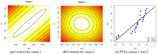
Figure 2.
Visual fitting of the IW model from radiation data.
Briefly, using the complete radiation data sets (reported in Table 3), we highlight the superiority of the IW lifespan model by comparing its fitting results to five other lifetime models, namely
- Inverted-Kumaraswamy (IK()) by Abd AL-Fattah et al. [39];
- Inverted-Lomax (IL()) by Kleiber and Kotz [40];
- Inverted-Pham (IP()) by Alqasem et al. [41];
- Inverted Nadarajah-Haghighi (INH()) by Tahir et al. [42];
- Exponentiated inverted Weibull (EIW()) by Flaih et al. [43].
In particular, this comparison is made based on clear criteria, namely (i) negative log-likelihood (NLL); (ii) Akaike information (AI); (iii) consistent AI (CAI); (iv) Bayesian information (BI); (v) Hannan–Quinn information (HQI); and (vi) KS (p-value). Thus, in Table 5, the MLEs (along with their St.Ers) of , , and as well as the estimates criteria (i)–(vi) are listed.
Table 5.
Fitting analysis of the IW and others from radiation data.
Consequently, from the radiation analyzed data using both causes 1 and 2, the results summarized in Table 5 indicate that the IW distribution outperforms all other candidate models. This conclusion is substantiated by the fact that the IW model consistently yields the most favorable outcomes across nearly all criteria, demonstrating the lowest values of all suggested metrics except the highest p-value.
Utilizing Table 3, three IAPTIIC competing risk samples are generated with under various combinations of and (see Table 6). The point estimation findings (along with their corresponding St.Ers) of , , and include both likelihood and Bayesian inferences obtained; see Table 7. In the same table, 95% ACI/HPD interval limits (along with their corresponding ILs) are computed. By performing 10,000 MCMC iterations as a burn-in from , Bayesian computations are performed. A comparative analysis in Table 7 reveals that the Bayesian MCMC estimates consistently outperform the likelihood-based results in terms of lower standard errors and narrower interval widths, indicating enhanced precision. Again, from for , the estimated relative risks (ERRs) due to causes 1 and 2 using the invariance property of and , are computed and reported in Table 7.
Table 6.
Three IAPTIIC competing risks from radiation data.
Table 7.
Estimates of , (for ), and from radiation data.
We noticed that, from Table 7, the ERR outcomes related to cause 1 increased when the removals were done in the last stages compared to the first (or middle stages), while those related to cause 2 increased when the removals were done in the first stages compared to the last (or middle) stages.
Furthermore, based on all samples listed in Table 3, Figure 3 presents the profile log-likelihood curves of and . The results support the fitted values provided in Table 7, demonstrating that the fitted MLEs and of and , respectively, exist and are unique, confirming the stability and reliability of the estimation process.
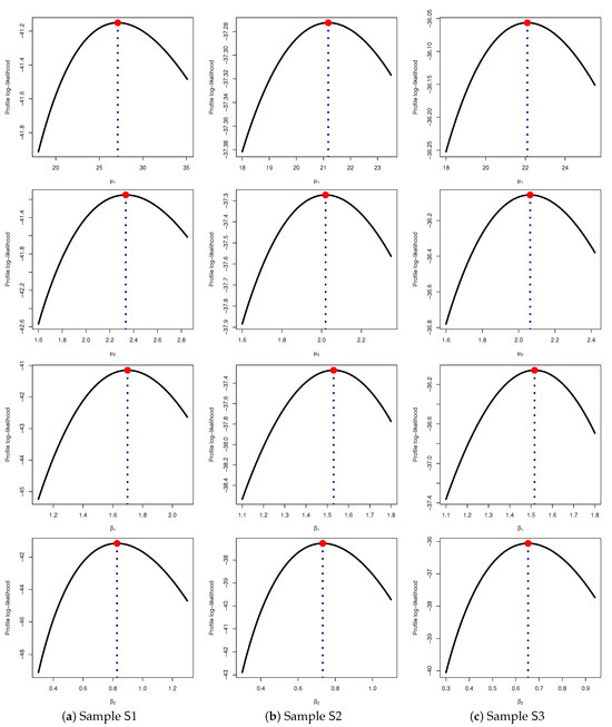
Figure 3.
Profile log-likelihoods for and (for ) from radiation data.
To assess the convergence behavior and mixing efficiency of the acquired remaining 30,000 MCMC iterations of , (for ), and from radiation data, both density and trace plots of the estimated parameters are generated for each sampled data set listed in Table 3. These visual diagnostics are presented in Figure 4. It indicates that for all unknown parameters , (for ), and , the posterior density functions exhibit near-symmetry as their normal proposals. Additionally, the trace plots demonstrate effective mixing, confirming that the Markov chains have achieved convergence, ensuring the reliability of the Bayesian inference.
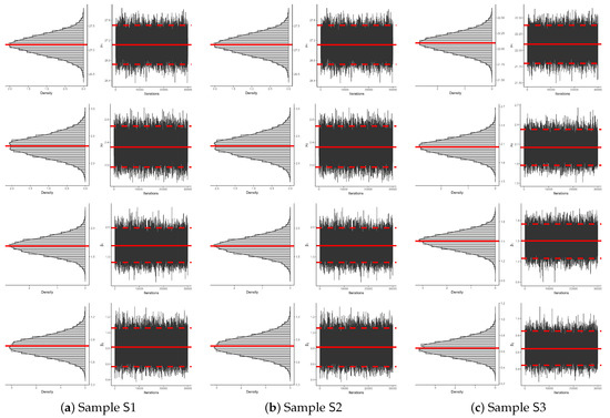
Figure 4.
Two MCMC plots of , (for ), and from radiation data.
7. Concluding Remarks
This study addressed the challenge of estimating unknown parameters and the reliability function of the inverted-Weibull distribution under improved adaptive progressively Type-II censored competing risks data. By employing both classical and Bayesian estimation approaches, the research provided a robust framework for reliability analysis in the presence of competing risks. The classical framework employs maximum likelihood estimation to derive point estimates and approximate confidence intervals, while the Bayesian approach utilizes Markov Chain Monte Carlo techniques to compute Bayes estimates and the highest posterior density credible intervals. A comprehensive simulation study demonstrated the accuracy and efficiency of the proposed methods across various experimental scenarios, highlighting their practical applicability. It evaluates estimators using metrics such as RMSE, MRAB, AIL, and CP across varied scenarios involving sample sizes, censoring rates, and time thresholds. The simulations, which were repeated 1000 times for each scenario, confirm the high accuracy and reliability of Bayesian methods based on the Metropolis–Hastings algorithm compared to traditional methods. The proposed point and interval estimation methods perform well under left- and right-censoring for cases and , respectively, while middle-censoring is the ideal for the reliability index . A significant radiation application is analyzed from a practical perspective to demonstrate the feasibility of the suggested approaches. In summary, the research findings using data sets from the radiobiology sector provide valuable insights into the inverted-Weibull lifetime model, particularly when an improved adaptive progressive censored competing risk data set is constructed. One limitation of the current study is the assumption of independence among latent failure times, which may not be appropriate when the causes of failure are correlated. In such cases, a dependent competing risks model would be more suitable for analyzing the data. Another limitation concerns the use of the improved adaptive progressive Type-II censoring scheme, which is most effective when the units under study have long lifespans. If the duration of the experiment is not a major constraint, traditional censoring schemes, such as the standard progressive Type-II censoring, may be more appropriate. Finally, the Bayesian estimation approach, while flexible and informative, is computationally intensive and more costly. In scenarios where prior information about the unknown parameters is unavailable, it is advisable to use classical estimation methods to reduce computational burden and save time. As a direction for future research, it would be valuable to compare the inverted Weibull model with alternative lifetime distributions or machine learning-based approaches to address situations where the true underlying distribution is unknown; see Meyer et al. [44] for additional details.
Author Contributions
Methodology, R.A., M.N. and A.E.; Funding acquisition, R.A.; Software, A.E.; Supervision M.N.; Writing—original draft, M.N. and A.E.; Writing—review & editing R.A. and M.N. All authors have read and agreed to the published version of the manuscript.
Funding
This research was funded by Princess Nourah bint Abdulrahman University Researchers Supporting Project number (PNURSP2025R50), Princess Nourah bint Abdulrahman University, Riyadh, Saudi Arabia.
Data Availability Statement
The authors confirm that the data supporting the findings of this study are available within the article.
Conflicts of Interest
The authors declare no conflicts of interest.
Appendix A. Simulation Tables
In this part, all simulation results of , , and are presented.
Table A1.
The point estimation results of .
Table A1.
The point estimation results of .
| n | Removals | MLE | Bayes | |||||||
|---|---|---|---|---|---|---|---|---|---|---|
| Prior-1 | Prior-2 | |||||||||
| 40 | [1] | 2.024 | 3.986 | 1.693 | 2.433 | 1.333 | 0.815 | 1.818 | 0.997 | 0.623 |
| [2] | 2.050 | 4.250 | 1.738 | 1.605 | 1.408 | 0.849 | 1.891 | 1.031 | 0.645 | |
| [3] | 1.995 | 4.528 | 1.761 | 1.559 | 1.562 | 0.921 | 1.633 | 1.112 | 0.690 | |
| [4] | 1.961 | 3.298 | 1.548 | 1.890 | 1.115 | 0.685 | 1.372 | 0.915 | 0.566 | |
| [5] | 2.224 | 3.698 | 1.688 | 1.994 | 1.294 | 0.757 | 1.859 | 0.987 | 0.600 | |
| [6] | 2.219 | 3.467 | 1.611 | 1.986 | 1.239 | 0.700 | 1.678 | 0.946 | 0.581 | |
| 60 | [1] | 2.259 | 2.338 | 1.417 | 2.085 | 0.984 | 0.611 | 1.377 | 0.758 | 0.457 |
| [2] | 2.369 | 2.698 | 1.463 | 2.111 | 1.030 | 0.632 | 1.867 | 0.822 | 0.501 | |
| [3] | 2.430 | 2.983 | 1.515 | 2.129 | 1.090 | 0.659 | 1.886 | 0.877 | 0.524 | |
| [4] | 1.994 | 1.925 | 1.239 | 2.020 | 0.808 | 0.521 | 1.532 | 0.636 | 0.383 | |
| [5] | 2.525 | 2.141 | 1.365 | 2.348 | 0.872 | 0.580 | 1.758 | 0.752 | 0.449 | |
| [6] | 2.497 | 1.988 | 1.313 | 2.366 | 0.838 | 0.558 | 1.264 | 0.645 | 0.396 | |
| 80 | [1] | 2.239 | 1.770 | 0.942 | 2.205 | 0.635 | 0.436 | 1.772 | 0.521 | 0.309 |
| [2] | 2.705 | 1.836 | 0.985 | 2.533 | 0.674 | 0.487 | 1.539 | 0.572 | 0.347 | |
| [3] | 2.618 | 1.886 | 1.159 | 2.466 | 0.725 | 0.509 | 1.430 | 0.628 | 0.374 | |
| [4] | 2.391 | 1.574 | 0.745 | 1.959 | 0.555 | 0.313 | 1.299 | 0.325 | 0.162 | |
| [5] | 2.714 | 1.610 | 0.885 | 2.283 | 0.601 | 0.403 | 1.159 | 0.430 | 0.267 | |
| [6] | 2.842 | 1.595 | 0.789 | 2.373 | 0.561 | 0.359 | 1.399 | 0.384 | 0.181 | |
| 40 | [1] | 2.662 | 4.192 | 1.817 | 2.166 | 1.225 | 0.876 | 1.417 | 1.026 | 0.630 |
| [2] | 1.728 | 4.359 | 1.982 | 2.057 | 1.474 | 0.909 | 1.622 | 1.133 | 0.683 | |
| [3] | 1.968 | 4.703 | 2.083 | 1.968 | 1.564 | 0.969 | 1.540 | 1.255 | 0.762 | |
| [4] | 2.064 | 3.648 | 1.542 | 2.064 | 1.060 | 0.687 | 1.433 | 0.932 | 0.562 | |
| [5] | 2.097 | 3.977 | 1.696 | 2.097 | 1.207 | 0.760 | 1.883 | 1.006 | 0.624 | |
| [6] | 2.167 | 3.751 | 1.641 | 2.167 | 1.174 | 0.716 | 1.595 | 0.976 | 0.612 | |
| 60 | [1] | 2.357 | 2.900 | 1.513 | 2.136 | 0.946 | 0.606 | 2.111 | 0.790 | 0.514 |
| [2] | 2.357 | 3.180 | 1.520 | 2.357 | 0.963 | 0.626 | 1.855 | 0.885 | 0.547 | |
| [3] | 2.268 | 3.449 | 1.538 | 2.268 | 1.022 | 0.641 | 1.584 | 0.902 | 0.552 | |
| [4] | 2.152 | 2.515 | 1.434 | 2.152 | 0.858 | 0.548 | 1.380 | 0.653 | 0.387 | |
| [5] | 2.458 | 2.765 | 1.503 | 2.046 | 0.926 | 0.594 | 1.550 | 0.750 | 0.478 | |
| [6] | 2.493 | 2.645 | 1.442 | 2.249 | 0.899 | 0.557 | 2.134 | 0.720 | 0.428 | |
| 80 | [1] | 2.384 | 2.233 | 1.347 | 2.384 | 0.686 | 0.424 | 1.805 | 0.503 | 0.292 |
| [2] | 2.637 | 2.337 | 1.414 | 2.637 | 0.728 | 0.441 | 1.591 | 0.517 | 0.300 | |
| [3] | 2.610 | 2.411 | 1.428 | 2.610 | 0.757 | 0.483 | 2.448 | 0.570 | 0.337 | |
| [4] | 2.334 | 1.863 | 1.205 | 2.033 | 0.518 | 0.330 | 1.948 | 0.311 | 0.160 | |
| [5] | 2.863 | 2.129 | 1.303 | 2.163 | 0.642 | 0.390 | 2.044 | 0.466 | 0.290 | |
| [6] | 2.768 | 2.021 | 1.294 | 2.027 | 0.611 | 0.377 | 1.445 | 0.363 | 0.169 | |
Table A2.
The point estimation results of .
Table A2.
The point estimation results of .
| n | Removals | MLE | Bayes | |||||||
|---|---|---|---|---|---|---|---|---|---|---|
| Prior-1 | Prior-2 | |||||||||
| 40 | [1] | 0.780 | 0.659 | 1.174 | 0.479 | 0.466 | 0.892 | 0.470 | 0.386 | 0.735 |
| [2] | 0.760 | 0.686 | 1.187 | 0.586 | 0.478 | 0.986 | 0.466 | 0.395 | 0.757 | |
| [3] | 0.740 | 0.724 | 1.227 | 0.551 | 0.526 | 1.007 | 0.417 | 0.424 | 0.824 | |
| [4] | 0.699 | 0.593 | 1.146 | 0.512 | 0.438 | 0.854 | 0.459 | 0.364 | 0.704 | |
| [5] | 0.712 | 0.626 | 1.163 | 0.462 | 0.456 | 0.882 | 0.417 | 0.375 | 0.720 | |
| [6] | 0.734 | 0.606 | 1.156 | 0.504 | 0.449 | 0.878 | 0.450 | 0.372 | 0.711 | |
| 60 | [1] | 0.748 | 0.576 | 1.125 | 0.588 | 0.386 | 0.822 | 0.531 | 0.340 | 0.646 |
| [2] | 0.748 | 0.577 | 1.131 | 0.588 | 0.405 | 0.835 | 0.531 | 0.344 | 0.652 | |
| [3] | 0.729 | 0.583 | 1.139 | 0.531 | 0.425 | 0.844 | 0.483 | 0.357 | 0.672 | |
| [4] | 0.706 | 0.560 | 1.102 | 0.547 | 0.329 | 0.727 | 0.525 | 0.312 | 0.607 | |
| [5] | 0.705 | 0.570 | 1.120 | 0.533 | 0.363 | 0.792 | 0.456 | 0.335 | 0.635 | |
| [6] | 0.726 | 0.565 | 1.113 | 0.571 | 0.336 | 0.745 | 0.493 | 0.323 | 0.623 | |
| 80 | [1] | 0.754 | 0.541 | 1.078 | 0.608 | 0.305 | 0.643 | 0.582 | 0.258 | 0.578 |
| [2] | 0.736 | 0.549 | 1.090 | 0.611 | 0.319 | 0.662 | 0.535 | 0.285 | 0.586 | |
| [3] | 0.718 | 0.551 | 1.098 | 0.578 | 0.320 | 0.697 | 0.503 | 0.297 | 0.599 | |
| [4] | 0.680 | 0.522 | 1.027 | 0.670 | 0.276 | 0.566 | 0.521 | 0.195 | 0.501 | |
| [5] | 0.692 | 0.538 | 1.065 | 0.608 | 0.298 | 0.602 | 0.484 | 0.238 | 0.567 | |
| [6] | 0.712 | 0.529 | 1.045 | 0.606 | 0.282 | 0.584 | 0.490 | 0.219 | 0.531 | |
| 40 | [1] | 0.771 | 1.387 | 1.248 | 0.468 | 0.518 | 0.926 | 0.450 | 0.404 | 0.749 |
| [2] | 0.791 | 1.640 | 1.249 | 0.630 | 0.537 | 0.944 | 0.493 | 0.427 | 0.794 | |
| [3] | 0.803 | 1.765 | 1.272 | 0.591 | 0.545 | 1.038 | 0.442 | 0.479 | 0.830 | |
| [4] | 0.749 | 0.962 | 1.226 | 0.504 | 0.455 | 0.880 | 0.445 | 0.368 | 0.708 | |
| [5] | 0.782 | 1.134 | 1.234 | 0.527 | 0.497 | 0.904 | 0.467 | 0.381 | 0.722 | |
| [6] | 0.774 | 0.996 | 1.230 | 0.530 | 0.476 | 0.895 | 0.466 | 0.375 | 0.716 | |
| 60 | [1] | 0.764 | 0.856 | 1.211 | 0.587 | 0.425 | 0.823 | 0.518 | 0.349 | 0.671 |
| [2] | 0.784 | 0.918 | 1.215 | 0.604 | 0.428 | 0.839 | 0.544 | 0.357 | 0.689 | |
| [3] | 0.791 | 0.946 | 1.216 | 0.563 | 0.432 | 0.843 | 0.512 | 0.361 | 0.691 | |
| [4] | 0.736 | 0.732 | 1.194 | 0.539 | 0.389 | 0.786 | 0.511 | 0.317 | 0.643 | |
| [5] | 0.772 | 0.815 | 1.208 | 0.578 | 0.417 | 0.809 | 0.488 | 0.343 | 0.667 | |
| [6] | 0.770 | 0.786 | 1.207 | 0.583 | 0.396 | 0.799 | 0.502 | 0.330 | 0.653 | |
| 80 | [1] | 0.755 | 0.639 | 1.177 | 0.607 | 0.360 | 0.690 | 0.579 | 0.281 | 0.578 |
| [2] | 0.775 | 0.660 | 1.181 | 0.628 | 0.371 | 0.729 | 0.545 | 0.298 | 0.599 | |
| [3] | 0.779 | 0.699 | 1.183 | 0.609 | 0.375 | 0.748 | 0.520 | 0.308 | 0.610 | |
| [4] | 0.732 | 0.572 | 1.130 | 0.686 | 0.317 | 0.590 | 0.522 | 0.265 | 0.545 | |
| [5] | 0.758 | 0.609 | 1.164 | 0.588 | 0.358 | 0.676 | 0.456 | 0.279 | 0.567 | |
| [6] | 0.757 | 0.586 | 1.139 | 0.639 | 0.331 | 0.625 | 0.500 | 0.271 | 0.557 | |
Table A3.
The point estimation results of .
Table A3.
The point estimation results of .
| n | Removals | MLE | Bayes | |||||||
|---|---|---|---|---|---|---|---|---|---|---|
| Prior-1 | Prior-2 | |||||||||
| 40 | [1] | 0.765 | 1.415 | 1.255 | 0.433 | 0.407 | 0.549 | 0.606 | 0.348 | 0.470 |
| [2] | 0.575 | 1.626 | 1.629 | 0.485 | 0.526 | 0.628 | 0.850 | 0.422 | 0.556 | |
| [3] | 0.657 | 1.325 | 1.206 | 0.644 | 0.398 | 0.539 | 0.604 | 0.340 | 0.443 | |
| [4] | 0.595 | 1.214 | 1.182 | 0.432 | 0.390 | 0.528 | 0.476 | 0.327 | 0.428 | |
| [5] | 0.572 | 1.103 | 0.953 | 0.376 | 0.380 | 0.505 | 0.424 | 0.308 | 0.421 | |
| [6] | 0.673 | 0.981 | 0.939 | 0.529 | 0.361 | 0.467 | 0.414 | 0.305 | 0.420 | |
| 60 | [1] | 0.822 | 0.759 | 0.866 | 0.516 | 0.348 | 0.460 | 0.516 | 0.294 | 0.414 |
| [2] | 0.758 | 0.824 | 0.913 | 0.489 | 0.349 | 0.462 | 0.538 | 0.303 | 0.414 | |
| [3] | 0.707 | 0.668 | 0.836 | 0.460 | 0.342 | 0.452 | 0.388 | 0.286 | 0.406 | |
| [4] | 0.765 | 0.576 | 0.827 | 0.366 | 0.337 | 0.436 | 0.447 | 0.284 | 0.375 | |
| [5] | 0.736 | 0.546 | 0.801 | 0.373 | 0.325 | 0.432 | 0.431 | 0.271 | 0.356 | |
| [6] | 0.741 | 0.489 | 0.711 | 0.515 | 0.323 | 0.423 | 0.617 | 0.258 | 0.347 | |
| 80 | [1] | 0.855 | 0.444 | 0.631 | 0.389 | 0.314 | 0.420 | 0.452 | 0.230 | 0.339 |
| [2] | 0.873 | 0.467 | 0.652 | 0.481 | 0.317 | 0.422 | 0.540 | 0.246 | 0.346 | |
| [3] | 0.728 | 0.424 | 0.587 | 0.525 | 0.301 | 0.414 | 0.598 | 0.228 | 0.284 | |
| [4] | 0.817 | 0.341 | 0.549 | 0.511 | 0.295 | 0.408 | 0.477 | 0.219 | 0.278 | |
| [5] | 0.739 | 0.324 | 0.557 | 0.413 | 0.277 | 0.398 | 0.407 | 0.214 | 0.271 | |
| [6] | 0.774 | 0.308 | 0.516 | 0.392 | 0.264 | 0.337 | 0.475 | 0.208 | 0.259 | |
| 40 | [1] | 1.224 | 1.024 | 1.511 | 0.447 | 0.386 | 0.523 | 0.661 | 0.368 | 0.502 |
| [2] | 1.069 | 1.181 | 1.658 | 0.555 | 0.448 | 0.568 | 0.866 | 0.425 | 0.535 | |
| [3] | 1.156 | 0.924 | 1.367 | 0.682 | 0.371 | 0.485 | 0.745 | 0.358 | 0.453 | |
| [4] | 0.998 | 0.883 | 1.367 | 0.513 | 0.368 | 0.465 | 0.535 | 0.334 | 0.446 | |
| [5] | 1.078 | 0.783 | 1.336 | 0.530 | 0.356 | 0.453 | 0.526 | 0.326 | 0.439 | |
| [6] | 0.933 | 0.725 | 1.292 | 0.505 | 0.354 | 0.428 | 0.413 | 0.315 | 0.424 | |
| 60 | [1] | 1.172 | 0.694 | 1.191 | 0.698 | 0.336 | 0.416 | 0.661 | 0.295 | 0.402 |
| [2] | 1.055 | 0.710 | 1.205 | 0.680 | 0.342 | 0.425 | 0.679 | 0.301 | 0.410 | |
| [3] | 1.172 | 0.682 | 1.183 | 0.698 | 0.333 | 0.404 | 0.661 | 0.284 | 0.399 | |
| [4] | 1.021 | 0.672 | 1.177 | 0.419 | 0.331 | 0.389 | 0.487 | 0.278 | 0.387 | |
| [5] | 1.091 | 0.669 | 1.132 | 0.527 | 0.323 | 0.379 | 0.553 | 0.273 | 0.372 | |
| [6] | 0.880 | 0.656 | 1.121 | 0.598 | 0.313 | 0.371 | 0.635 | 0.267 | 0.362 | |
| 80 | [1] | 1.139 | 0.601 | 1.097 | 0.537 | 0.285 | 0.358 | 0.562 | 0.259 | 0.343 |
| [2] | 1.064 | 0.638 | 1.099 | 0.539 | 0.291 | 0.367 | 0.568 | 0.260 | 0.350 | |
| [3] | 1.048 | 0.567 | 1.022 | 0.576 | 0.277 | 0.351 | 0.613 | 0.249 | 0.330 | |
| [4] | 1.004 | 0.556 | 0.935 | 0.488 | 0.257 | 0.345 | 0.447 | 0.222 | 0.320 | |
| [5] | 1.049 | 0.475 | 0.880 | 0.465 | 0.237 | 0.318 | 0.434 | 0.188 | 0.240 | |
| [6] | 0.940 | 0.426 | 0.763 | 0.723 | 0.220 | 0.297 | 0.700 | 0.175 | 0.236 | |
Table A4.
The point estimation results of .
Table A4.
The point estimation results of .
| n | Removals | MLE | Bayes | |||||||
|---|---|---|---|---|---|---|---|---|---|---|
| Prior-1 | Prior-2 | |||||||||
| 40 | [1] | 1.497 | 0.716 | 0.519 | 0.970 | 0.684 | 0.442 | 1.196 | 0.549 | 0.335 |
| [2] | 1.441 | 0.616 | 0.425 | 0.838 | 0.572 | 0.386 | 0.997 | 0.535 | 0.325 | |
| [3] | 1.188 | 0.607 | 0.370 | 1.653 | 0.544 | 0.324 | 1.371 | 0.499 | 0.275 | |
| [4] | 1.214 | 0.522 | 0.317 | 0.999 | 0.457 | 0.263 | 1.090 | 0.424 | 0.256 | |
| [5] | 1.332 | 0.550 | 0.335 | 1.137 | 0.471 | 0.290 | 1.203 | 0.440 | 0.267 | |
| [6] | 1.273 | 0.511 | 0.285 | 1.124 | 0.442 | 0.226 | 1.299 | 0.402 | 0.215 | |
| 60 | [1] | 1.437 | 0.480 | 0.261 | 1.236 | 0.410 | 0.225 | 1.281 | 0.383 | 0.214 |
| [2] | 1.359 | 0.455 | 0.245 | 0.921 | 0.395 | 0.221 | 1.012 | 0.371 | 0.204 | |
| [3] | 1.179 | 0.439 | 0.227 | 1.206 | 0.388 | 0.219 | 1.285 | 0.357 | 0.181 | |
| [4] | 1.216 | 0.404 | 0.209 | 1.178 | 0.372 | 0.197 | 1.256 | 0.347 | 0.167 | |
| [5] | 1.352 | 0.422 | 0.222 | 1.293 | 0.379 | 0.218 | 1.402 | 0.349 | 0.170 | |
| [6] | 1.247 | 0.397 | 0.189 | 1.025 | 0.367 | 0.186 | 1.099 | 0.346 | 0.162 | |
| 80 | [1] | 1.426 | 0.386 | 0.183 | 1.411 | 0.356 | 0.173 | 1.497 | 0.305 | 0.148 |
| [2] | 1.362 | 0.376 | 0.179 | 1.292 | 0.341 | 0.159 | 1.362 | 0.296 | 0.141 | |
| [3] | 1.176 | 0.365 | 0.176 | 1.074 | 0.333 | 0.149 | 1.117 | 0.295 | 0.137 | |
| [4] | 1.185 | 0.352 | 0.163 | 1.351 | 0.310 | 0.138 | 1.181 | 0.278 | 0.125 | |
| [5] | 1.313 | 0.359 | 0.167 | 1.546 | 0.328 | 0.141 | 1.327 | 0.284 | 0.134 | |
| [6] | 1.242 | 0.343 | 0.142 | 1.244 | 0.308 | 0.131 | 1.340 | 0.264 | 0.122 | |
| 40 | [1] | 1.886 | 0.696 | 0.341 | 1.098 | 0.527 | 0.292 | 1.284 | 0.468 | 0.287 |
| [2] | 1.946 | 0.638 | 0.332 | 1.116 | 0.491 | 0.288 | 1.234 | 0.436 | 0.240 | |
| [3] | 1.655 | 0.579 | 0.288 | 1.789 | 0.490 | 0.273 | 1.841 | 0.399 | 0.205 | |
| [4] | 1.772 | 0.525 | 0.262 | 1.188 | 0.468 | 0.253 | 1.222 | 0.379 | 0.186 | |
| [5] | 1.797 | 0.543 | 0.276 | 1.263 | 0.477 | 0.267 | 1.300 | 0.388 | 0.204 | |
| [6] | 1.651 | 0.513 | 0.256 | 1.376 | 0.453 | 0.247 | 1.451 | 0.367 | 0.186 | |
| 60 | [1] | 1.814 | 0.511 | 0.252 | 1.278 | 0.407 | 0.219 | 1.321 | 0.361 | 0.182 |
| [2] | 1.867 | 0.472 | 0.245 | 1.253 | 0.384 | 0.197 | 1.275 | 0.344 | 0.179 | |
| [3] | 1.867 | 0.469 | 0.240 | 1.253 | 0.375 | 0.186 | 1.275 | 0.331 | 0.172 | |
| [4] | 1.767 | 0.445 | 0.223 | 1.571 | 0.336 | 0.167 | 1.562 | 0.318 | 0.154 | |
| [5] | 1.797 | 0.455 | 0.231 | 1.663 | 0.338 | 0.171 | 1.676 | 0.326 | 0.165 | |
| [6] | 1.514 | 0.421 | 0.216 | 1.371 | 0.333 | 0.167 | 1.342 | 0.310 | 0.138 | |
| 80 | [1] | 1.797 | 0.381 | 0.201 | 1.752 | 0.315 | 0.162 | 1.746 | 0.292 | 0.128 |
| [2] | 1.837 | 0.377 | 0.198 | 1.565 | 0.309 | 0.150 | 1.561 | 0.280 | 0.120 | |
| [3] | 1.658 | 0.341 | 0.179 | 1.381 | 0.303 | 0.148 | 1.351 | 0.260 | 0.117 | |
| [4] | 1.733 | 0.316 | 0.153 | 1.757 | 0.281 | 0.136 | 1.478 | 0.255 | 0.101 | |
| [5] | 1.759 | 0.329 | 0.167 | 1.835 | 0.293 | 0.142 | 1.563 | 0.257 | 0.110 | |
| [6] | 1.632 | 0.282 | 0.147 | 1.596 | 0.260 | 0.129 | 1.584 | 0.184 | 0.093 | |
Table A5.
The point estimation results of .
Table A5.
The point estimation results of .
| n | Removals | MLE | Bayes | |||||||
|---|---|---|---|---|---|---|---|---|---|---|
| Prior-1 | Prior-2 | |||||||||
| 40 | [1] | 0.973 | 0.185 | 0.241 | 0.962 | 0.127 | 0.185 | 0.985 | 0.115 | 0.064 |
| [2] | 0.992 | 0.175 | 0.195 | 0.981 | 0.116 | 0.157 | 0.992 | 0.093 | 0.056 | |
| [3] | 0.983 | 0.178 | 0.229 | 0.958 | 0.121 | 0.168 | 0.958 | 0.106 | 0.059 | |
| [4] | 0.983 | 0.160 | 0.179 | 0.972 | 0.111 | 0.125 | 0.967 | 0.084 | 0.056 | |
| [5] | 0.991 | 0.148 | 0.148 | 0.960 | 0.105 | 0.089 | 0.952 | 0.068 | 0.053 | |
| [6] | 0.983 | 0.156 | 0.168 | 0.962 | 0.109 | 0.105 | 0.956 | 0.075 | 0.054 | |
| 60 | [1] | 0.986 | 0.143 | 0.138 | 0.984 | 0.095 | 0.082 | 0.981 | 0.062 | 0.052 |
| [2] | 0.986 | 0.132 | 0.122 | 0.970 | 0.075 | 0.070 | 0.960 | 0.050 | 0.048 | |
| [3] | 0.992 | 0.137 | 0.128 | 0.982 | 0.084 | 0.078 | 0.974 | 0.055 | 0.050 | |
| [4] | 0.981 | 0.127 | 0.115 | 0.974 | 0.066 | 0.064 | 0.972 | 0.047 | 0.048 | |
| [5] | 0.992 | 0.107 | 0.102 | 0.961 | 0.054 | 0.049 | 0.983 | 0.039 | 0.045 | |
| [6] | 0.983 | 0.117 | 0.108 | 0.973 | 0.060 | 0.054 | 0.971 | 0.044 | 0.045 | |
| 80 | [1] | 0.948 | 0.096 | 0.096 | 0.990 | 0.051 | 0.049 | 0.982 | 0.035 | 0.038 |
| [2] | 0.954 | 0.082 | 0.087 | 0.984 | 0.048 | 0.046 | 0.988 | 0.031 | 0.035 | |
| [3] | 0.958 | 0.086 | 0.092 | 0.990 | 0.050 | 0.048 | 0.977 | 0.034 | 0.037 | |
| [4] | 0.982 | 0.077 | 0.082 | 0.986 | 0.047 | 0.044 | 0.979 | 0.028 | 0.032 | |
| [5] | 0.933 | 0.067 | 0.072 | 0.995 | 0.041 | 0.038 | 0.962 | 0.022 | 0.028 | |
| [6] | 0.966 | 0.071 | 0.076 | 0.984 | 0.046 | 0.041 | 0.974 | 0.026 | 0.031 | |
| 40 | [1] | 0.979 | 0.152 | 0.178 | 0.972 | 0.097 | 0.095 | 0.986 | 0.082 | 0.063 |
| [2] | 0.958 | 0.136 | 0.154 | 0.994 | 0.073 | 0.081 | 0.995 | 0.069 | 0.059 | |
| [3] | 0.961 | 0.143 | 0.167 | 0.964 | 0.083 | 0.087 | 0.969 | 0.076 | 0.060 | |
| [4] | 0.977 | 0.129 | 0.143 | 0.978 | 0.069 | 0.077 | 0.969 | 0.066 | 0.057 | |
| [5] | 0.987 | 0.114 | 0.129 | 0.967 | 0.062 | 0.065 | 0.956 | 0.057 | 0.051 | |
| [6] | 0.988 | 0.124 | 0.137 | 0.981 | 0.065 | 0.070 | 0.970 | 0.062 | 0.054 | |
| 60 | [1] | 0.989 | 0.110 | 0.124 | 0.993 | 0.061 | 0.062 | 0.989 | 0.051 | 0.049 |
| [2] | 0.945 | 0.098 | 0.112 | 0.994 | 0.058 | 0.057 | 0.988 | 0.043 | 0.040 | |
| [3] | 0.954 | 0.105 | 0.117 | 0.994 | 0.059 | 0.058 | 0.988 | 0.048 | 0.044 | |
| [4] | 0.995 | 0.087 | 0.108 | 0.978 | 0.057 | 0.056 | 0.975 | 0.041 | 0.037 | |
| [5] | 0.982 | 0.078 | 0.099 | 0.979 | 0.053 | 0.052 | 0.989 | 0.035 | 0.030 | |
| [6] | 0.955 | 0.079 | 0.102 | 0.987 | 0.055 | 0.054 | 0.980 | 0.038 | 0.034 | |
| 80 | [1] | 0.987 | 0.074 | 0.094 | 0.987 | 0.050 | 0.044 | 0.983 | 0.032 | 0.028 |
| [2] | 0.979 | 0.067 | 0.083 | 0.974 | 0.043 | 0.042 | 0.991 | 0.027 | 0.023 | |
| [3] | 0.990 | 0.071 | 0.087 | 0.981 | 0.046 | 0.043 | 0.984 | 0.030 | 0.025 | |
| [4] | 0.991 | 0.062 | 0.079 | 0.986 | 0.041 | 0.039 | 0.981 | 0.024 | 0.022 | |
| [5] | 0.972 | 0.057 | 0.072 | 0.972 | 0.036 | 0.033 | 0.987 | 0.019 | 0.018 | |
| [6] | 0.980 | 0.059 | 0.075 | 0.980 | 0.037 | 0.035 | 0.980 | 0.022 | 0.021 | |
Table A6.
The 95% interval estimation results of .
Table A6.
The 95% interval estimation results of .
| n | Removals | (1.25, 1.75) | (1.75, 2.50) | ||||||||||
|---|---|---|---|---|---|---|---|---|---|---|---|---|---|
| ACI | HPD | ACI | HPD | ||||||||||
| Prior-1 | Prior-2 | Prior-1 | Prior-2 | ||||||||||
| 40 | [1] | 2.268 | 0.937 | 1.563 | 0.942 | 1.335 | 0.948 | 2.330 | 0.935 | 1.844 | 0.939 | 1.415 | 0.944 |
| [2] | 2.326 | 0.936 | 1.795 | 0.941 | 1.384 | 0.948 | 2.447 | 0.934 | 2.199 | 0.938 | 1.472 | 0.944 | |
| [3] | 2.379 | 0.934 | 1.936 | 0.939 | 1.397 | 0.946 | 2.500 | 0.932 | 2.245 | 0.936 | 1.526 | 0.942 | |
| [4] | 1.943 | 0.942 | 1.463 | 0.948 | 1.299 | 0.953 | 2.079 | 0.940 | 1.583 | 0.944 | 1.325 | 0.949 | |
| [5] | 2.180 | 0.939 | 1.518 | 0.945 | 1.325 | 0.950 | 2.219 | 0.937 | 1.789 | 0.941 | 1.371 | 0.946 | |
| [6] | 2.045 | 0.941 | 1.492 | 0.947 | 1.306 | 0.952 | 2.175 | 0.939 | 1.656 | 0.943 | 1.339 | 0.948 | |
| 60 | [1] | 1.580 | 0.946 | 1.366 | 0.952 | 1.212 | 0.957 | 1.786 | 0.944 | 1.368 | 0.948 | 1.303 | 0.953 |
| [2] | 1.605 | 0.944 | 1.386 | 0.950 | 1.234 | 0.955 | 1.845 | 0.942 | 1.450 | 0.946 | 1.311 | 0.951 | |
| [3] | 1.872 | 0.942 | 1.424 | 0.948 | 1.245 | 0.953 | 1.999 | 0.940 | 1.527 | 0.944 | 1.314 | 0.949 | |
| [4] | 1.413 | 0.950 | 1.216 | 0.957 | 1.141 | 0.961 | 1.630 | 0.948 | 1.264 | 0.954 | 1.248 | 0.957 | |
| [5] | 1.524 | 0.947 | 1.318 | 0.953 | 1.194 | 0.958 | 1.725 | 0.945 | 1.345 | 0.949 | 1.283 | 0.954 | |
| [6] | 1.462 | 0.949 | 1.282 | 0.955 | 1.176 | 0.960 | 1.599 | 0.947 | 1.309 | 0.951 | 1.250 | 0.956 | |
| 80 | [1] | 1.296 | 0.954 | 1.019 | 0.960 | 0.980 | 0.965 | 1.348 | 0.952 | 1.142 | 0.956 | 1.025 | 0.961 |
| [2] | 1.327 | 0.953 | 1.086 | 0.959 | 1.062 | 0.964 | 1.422 | 0.951 | 1.194 | 0.955 | 1.175 | 0.960 | |
| [3] | 1.367 | 0.952 | 1.186 | 0.956 | 1.108 | 0.963 | 1.544 | 0.950 | 1.230 | 0.953 | 1.184 | 0.959 | |
| [4] | 0.985 | 0.958 | 0.728 | 0.964 | 0.664 | 0.969 | 1.013 | 0.956 | 0.817 | 0.960 | 0.671 | 0.965 | |
| [5] | 1.218 | 0.956 | 0.990 | 0.962 | 0.859 | 0.967 | 1.281 | 0.954 | 1.036 | 0.958 | 0.870 | 0.963 | |
| [6] | 1.034 | 0.957 | 0.813 | 0.961 | 0.795 | 0.968 | 1.127 | 0.955 | 0.942 | 0.958 | 0.842 | 0.964 | |
Table A7.
The 95% interval estimation results of .
Table A7.
The 95% interval estimation results of .
| n | Removals | (1.25, 1.75) | (1.75, 2.50) | ||||||||||
|---|---|---|---|---|---|---|---|---|---|---|---|---|---|
| ACI | HPD | ACI | HPD | ||||||||||
| Prior-1 | Prior-2 | Prior-1 | Prior-2 | ||||||||||
| 40 | [1] | 1.512 | 0.947 | 1.358 | 0.951 | 1.179 | 0.952 | 1.683 | 0.943 | 1.568 | 0.947 | 1.191 | 0.950 |
| [2] | 1.667 | 0.942 | 1.474 | 0.946 | 1.226 | 0.948 | 2.079 | 0.938 | 1.770 | 0.942 | 1.248 | 0.947 | |
| [3] | 1.585 | 0.944 | 1.417 | 0.948 | 1.194 | 0.949 | 1.826 | 0.940 | 1.740 | 0.944 | 1.237 | 0.947 | |
| [4] | 1.376 | 0.950 | 1.232 | 0.954 | 1.124 | 0.954 | 1.615 | 0.946 | 1.382 | 0.950 | 1.167 | 0.952 | |
| [5] | 1.437 | 0.949 | 1.258 | 0.953 | 1.141 | 0.953 | 1.666 | 0.945 | 1.433 | 0.949 | 1.178 | 0.950 | |
| [6] | 1.462 | 0.947 | 1.296 | 0.951 | 1.168 | 0.952 | 1.677 | 0.943 | 1.525 | 0.947 | 1.180 | 0.950 | |
| 60 | [1] | 1.200 | 0.957 | 1.177 | 0.958 | 1.073 | 0.961 | 1.332 | 0.953 | 1.290 | 0.954 | 1.083 | 0.959 |
| [2] | 1.318 | 0.952 | 1.217 | 0.955 | 1.107 | 0.956 | 1.546 | 0.948 | 1.321 | 0.951 | 1.147 | 0.954 | |
| [3] | 1.271 | 0.955 | 1.209 | 0.958 | 1.090 | 0.959 | 1.466 | 0.951 | 1.296 | 0.954 | 1.107 | 0.957 | |
| [4] | 1.115 | 0.958 | 1.108 | 0.961 | 1.033 | 0.962 | 1.307 | 0.954 | 1.247 | 0.957 | 1.022 | 0.960 | |
| [5] | 1.142 | 0.957 | 1.129 | 0.960 | 1.059 | 0.961 | 1.319 | 0.953 | 1.271 | 0.956 | 1.055 | 0.959 | |
| [6] | 1.166 | 0.957 | 1.154 | 0.960 | 1.071 | 0.961 | 1.328 | 0.953 | 1.278 | 0.956 | 1.060 | 0.959 | |
| 80 | [1] | 1.011 | 0.961 | 0.894 | 0.963 | 0.822 | 0.965 | 1.179 | 0.957 | 1.038 | 0.959 | 0.849 | 0.963 |
| [2] | 1.100 | 0.959 | 1.007 | 0.962 | 0.998 | 0.962 | 1.272 | 0.955 | 1.168 | 0.958 | 1.000 | 0.960 | |
| [3] | 1.014 | 0.960 | 0.968 | 0.962 | 0.929 | 0.963 | 1.218 | 0.956 | 1.114 | 0.958 | 0.997 | 0.961 | |
| [4] | 0.927 | 0.962 | 0.831 | 0.966 | 0.771 | 0.967 | 1.014 | 0.958 | 0.865 | 0.962 | 0.782 | 0.965 | |
| [5] | 0.961 | 0.961 | 0.852 | 0.964 | 0.795 | 0.967 | 1.125 | 0.957 | 0.901 | 0.960 | 0.798 | 0.964 | |
| [6] | 0.986 | 0.961 | 0.875 | 0.963 | 0.817 | 0.966 | 1.159 | 0.957 | 1.009 | 0.959 | 0.818 | 0.964 | |
Table A8.
The 95% interval estimation results of .
Table A8.
The 95% interval estimation results of .
| n | Removals | (1.25, 1.75) | (1.75, 2.50) | ||||||||||
|---|---|---|---|---|---|---|---|---|---|---|---|---|---|
| ACI | HPD | ACI | HPD | ||||||||||
| Prior-1 | Prior-2 | Prior-1 | Prior-2 | ||||||||||
| 40 | [1] | 1.964 | 0.929 | 1.350 | 0.942 | 1.050 | 0.946 | 1.682 | 0.933 | 1.107 | 0.946 | 0.925 | 0.947 |
| [2] | 2.188 | 0.927 | 1.419 | 0.940 | 1.137 | 0.944 | 1.874 | 0.931 | 1.134 | 0.944 | 0.996 | 0.945 | |
| [3] | 1.896 | 0.931 | 1.299 | 0.944 | 0.968 | 0.948 | 1.432 | 0.935 | 0.997 | 0.948 | 0.909 | 0.949 | |
| [4] | 1.681 | 0.934 | 1.250 | 0.945 | 0.944 | 0.949 | 1.394 | 0.938 | 0.987 | 0.949 | 0.896 | 0.951 | |
| [5] | 1.593 | 0.936 | 1.219 | 0.946 | 0.920 | 0.950 | 1.324 | 0.940 | 0.972 | 0.950 | 0.878 | 0.952 | |
| [6] | 1.347 | 0.939 | 1.186 | 0.948 | 0.906 | 0.951 | 1.265 | 0.943 | 0.967 | 0.952 | 0.854 | 0.953 | |
| 60 | [1] | 1.185 | 0.942 | 0.990 | 0.949 | 0.855 | 0.952 | 1.155 | 0.946 | 0.955 | 0.953 | 0.837 | 0.954 |
| [2] | 1.254 | 0.941 | 1.098 | 0.949 | 0.878 | 0.952 | 1.224 | 0.945 | 0.966 | 0.953 | 0.840 | 0.954 | |
| [3] | 1.174 | 0.943 | 0.987 | 0.949 | 0.837 | 0.952 | 1.057 | 0.947 | 0.939 | 0.953 | 0.814 | 0.954 | |
| [4] | 1.115 | 0.943 | 0.978 | 0.950 | 0.825 | 0.953 | 1.009 | 0.947 | 0.927 | 0.954 | 0.799 | 0.955 | |
| [5] | 1.005 | 0.944 | 0.937 | 0.951 | 0.803 | 0.954 | 0.987 | 0.948 | 0.921 | 0.955 | 0.784 | 0.956 | |
| [6] | 0.997 | 0.945 | 0.917 | 0.952 | 0.762 | 0.955 | 0.915 | 0.949 | 0.895 | 0.956 | 0.775 | 0.957 | |
| 80 | [1] | 0.902 | 0.946 | 0.887 | 0.953 | 0.726 | 0.956 | 0.832 | 0.950 | 0.795 | 0.957 | 0.732 | 0.958 |
| [2] | 0.943 | 0.946 | 0.907 | 0.952 | 0.759 | 0.955 | 0.892 | 0.950 | 0.826 | 0.956 | 0.745 | 0.957 | |
| [3] | 0.896 | 0.947 | 0.846 | 0.954 | 0.696 | 0.957 | 0.794 | 0.951 | 0.745 | 0.957 | 0.694 | 0.960 | |
| [4] | 0.884 | 0.948 | 0.779 | 0.956 | 0.669 | 0.957 | 0.763 | 0.952 | 0.685 | 0.959 | 0.678 | 0.960 | |
| [5] | 0.858 | 0.948 | 0.746 | 0.956 | 0.618 | 0.959 | 0.713 | 0.952 | 0.650 | 0.960 | 0.648 | 0.961 | |
| [6] | 0.835 | 0.949 | 0.710 | 0.957 | 0.585 | 0.960 | 0.675 | 0.953 | 0.627 | 0.961 | 0.573 | 0.963 | |
Table A9.
The 95% interval estimation results of .
Table A9.
The 95% interval estimation results of .
| n | Removals | (1.25, 1.75) | (1.75, 2.50) | ||||||||||
|---|---|---|---|---|---|---|---|---|---|---|---|---|---|
| ACI | HPD | ACI | HPD | ||||||||||
| Prior-1 | Prior-2 | Prior-1 | Prior-2 | ||||||||||
| 40 | [1] | 1.609 | 0.927 | 1.458 | 0.932 | 1.210 | 0.936 | 1.603 | 0.926 | 1.171 | 0.935 | 1.112 | 0.939 |
| [2] | 1.804 | 0.924 | 1.530 | 0.929 | 1.336 | 0.935 | 1.762 | 0.923 | 1.203 | 0.932 | 1.171 | 0.938 | |
| [3] | 1.596 | 0.929 | 1.410 | 0.932 | 1.164 | 0.938 | 1.548 | 0.928 | 1.144 | 0.937 | 0.990 | 0.941 | |
| [4] | 1.538 | 0.930 | 1.322 | 0.934 | 1.115 | 0.939 | 1.471 | 0.929 | 1.134 | 0.937 | 0.952 | 0.942 | |
| [5] | 1.406 | 0.931 | 1.267 | 0.936 | 1.017 | 0.939 | 1.386 | 0.930 | 1.104 | 0.939 | 0.942 | 0.942 | |
| [6] | 1.385 | 0.933 | 1.202 | 0.937 | 0.992 | 0.943 | 1.368 | 0.931 | 1.028 | 0.940 | 0.906 | 0.945 | |
| 60 | [1] | 1.319 | 0.934 | 1.108 | 0.938 | 0.929 | 0.944 | 1.268 | 0.934 | 1.012 | 0.941 | 0.876 | 0.946 |
| [2] | 1.348 | 0.934 | 1.138 | 0.937 | 0.969 | 0.944 | 1.309 | 0.933 | 1.024 | 0.940 | 0.891 | 0.946 | |
| [3] | 1.287 | 0.935 | 1.093 | 0.939 | 0.908 | 0.944 | 1.249 | 0.934 | 0.975 | 0.943 | 0.871 | 0.946 | |
| [4] | 1.239 | 0.936 | 1.057 | 0.939 | 0.873 | 0.945 | 1.214 | 0.935 | 0.928 | 0.944 | 0.842 | 0.948 | |
| [5] | 1.115 | 0.938 | 1.044 | 0.941 | 0.826 | 0.947 | 1.115 | 0.937 | 0.904 | 0.946 | 0.798 | 0.950 | |
| [6] | 1.096 | 0.939 | 0.927 | 0.942 | 0.789 | 0.949 | 1.106 | 0.937 | 0.883 | 0.947 | 0.753 | 0.951 | |
| 80 | [1] | 1.069 | 0.940 | 0.875 | 0.944 | 0.703 | 0.950 | 1.016 | 0.938 | 0.837 | 0.947 | 0.708 | 0.952 |
| [2] | 1.085 | 0.939 | 0.919 | 0.944 | 0.762 | 0.949 | 1.076 | 0.938 | 0.856 | 0.947 | 0.732 | 0.951 | |
| [3] | 1.066 | 0.940 | 0.828 | 0.944 | 0.695 | 0.950 | 0.986 | 0.939 | 0.827 | 0.948 | 0.696 | 0.952 | |
| [4] | 0.961 | 0.941 | 0.817 | 0.945 | 0.678 | 0.951 | 0.951 | 0.940 | 0.771 | 0.950 | 0.667 | 0.952 | |
| [5] | 0.919 | 0.941 | 0.805 | 0.945 | 0.653 | 0.951 | 0.902 | 0.940 | 0.701 | 0.951 | 0.639 | 0.953 | |
| [6] | 0.891 | 0.942 | 0.717 | 0.947 | 0.639 | 0.952 | 0.880 | 0.941 | 0.631 | 0.952 | 0.607 | 0.954 | |
Table A10.
The 95% interval estimation results of .
Table A10.
The 95% interval estimation results of .
| n | Removals | (1.25, 1.75) | (1.75, 2.50) | ||||||||||
|---|---|---|---|---|---|---|---|---|---|---|---|---|---|
| ACI | HPD | ACI | HPD | ||||||||||
| Prior-1 | Prior-2 | Prior-1 | Prior-2 | ||||||||||
| 40 | [1] | 0.416 | 0.942 | 0.217 | 0.949 | 0.139 | 0.953 | 0.375 | 0.945 | 0.136 | 0.952 | 0.102 | 0.954 |
| [2] | 0.337 | 0.947 | 0.159 | 0.954 | 0.095 | 0.957 | 0.300 | 0.948 | 0.109 | 0.955 | 0.084 | 0.959 | |
| [3] | 0.384 | 0.944 | 0.190 | 0.951 | 0.121 | 0.955 | 0.353 | 0.946 | 0.128 | 0.953 | 0.085 | 0.956 | |
| [4] | 0.313 | 0.948 | 0.129 | 0.956 | 0.090 | 0.958 | 0.269 | 0.950 | 0.098 | 0.956 | 0.079 | 0.960 | |
| [5] | 0.245 | 0.953 | 0.111 | 0.957 | 0.084 | 0.959 | 0.215 | 0.954 | 0.078 | 0.959 | 0.074 | 0.960 | |
| [6] | 0.277 | 0.951 | 0.118 | 0.957 | 0.089 | 0.958 | 0.240 | 0.952 | 0.087 | 0.958 | 0.076 | 0.960 | |
| 60 | [1] | 0.213 | 0.955 | 0.106 | 0.957 | 0.080 | 0.959 | 0.199 | 0.956 | 0.072 | 0.959 | 0.066 | 0.962 |
| [2] | 0.165 | 0.958 | 0.082 | 0.960 | 0.071 | 0.962 | 0.145 | 0.959 | 0.060 | 0.962 | 0.058 | 0.963 | |
| [3] | 0.186 | 0.957 | 0.095 | 0.958 | 0.075 | 0.960 | 0.173 | 0.957 | 0.068 | 0.960 | 0.061 | 0.962 | |
| [4] | 0.157 | 0.958 | 0.066 | 0.962 | 0.063 | 0.962 | 0.135 | 0.959 | 0.057 | 0.962 | 0.052 | 0.964 | |
| [5] | 0.121 | 0.960 | 0.061 | 0.963 | 0.051 | 0.964 | 0.100 | 0.961 | 0.044 | 0.963 | 0.043 | 0.965 | |
| [6] | 0.138 | 0.959 | 0.063 | 0.962 | 0.057 | 0.963 | 0.116 | 0.961 | 0.050 | 0.963 | 0.047 | 0.965 | |
| 80 | [1] | 0.111 | 0.960 | 0.055 | 0.963 | 0.045 | 0.965 | 0.086 | 0.963 | 0.040 | 0.964 | 0.039 | 0.966 |
| [2] | 0.093 | 0.962 | 0.045 | 0.964 | 0.035 | 0.966 | 0.070 | 0.964 | 0.034 | 0.966 | 0.031 | 0.967 | |
| [3] | 0.101 | 0.961 | 0.048 | 0.964 | 0.041 | 0.966 | 0.077 | 0.964 | 0.037 | 0.966 | 0.033 | 0.967 | |
| [4] | 0.082 | 0.962 | 0.042 | 0.965 | 0.032 | 0.967 | 0.059 | 0.965 | 0.030 | 0.967 | 0.023 | 0.968 | |
| [5] | 0.059 | 0.964 | 0.036 | 0.965 | 0.021 | 0.969 | 0.054 | 0.965 | 0.021 | 0.967 | 0.016 | 0.969 | |
| [6] | 0.068 | 0.963 | 0.040 | 0.965 | 0.026 | 0.968 | 0.058 | 0.965 | 0.025 | 0.967 | 0.019 | 0.968 | |
References
- Balakrishnan, N.; Kannan, N.; Lin, C.T.; Wu, S.J.S. Inference for the extreme value distribution under progressive Type-II censoring. J. Stat. Comput. Simul. 2004, 74, 25–45. [Google Scholar] [CrossRef]
- Balakrishnan, N.; Hossain, A. Inference for the Type II generalized logistic distribution under progressive Type II censoring. J. Stat. Comput. Simul. 2007, 77, 1013–1031. [Google Scholar] [CrossRef]
- Wu, M.; Gui, W. Estimation and prediction for Nadarajah-Haghighi distribution under progressive type-II censoring. Symmetry 2021, 13, 999. [Google Scholar] [CrossRef]
- Dey, S.; Elshahhat, A.; Nassar, M. Analysis of progressive type-II censored gamma distribution. Comput. Stat. 2023, 38, 481–508. [Google Scholar] [CrossRef]
- Ng, H.K.T.; Kundu, D.; Chan, P.S. Statistical analysis of exponential lifetimes under an adaptive Type-II progressive censoring scheme. Nav. Res. Logist. 2009, 56, 687–698. [Google Scholar] [CrossRef]
- Kundu, D.; Joarder, A. Analysis of Type-II progressively hybrid censored data. Comput. Stat. Data Anal. 2006, 50, 2509–2528. [Google Scholar] [CrossRef]
- Sobhi, M.M.A.; Soliman, A.A. Estimation for the exponentiated Weibull model with adaptive Type-II progressive censored schemes. Appl. Math. Model. 2016, 40, 1180–1192. [Google Scholar] [CrossRef]
- Kohansal, A.; Shoaee, S. Bayesian and classical estimation of reliability in a multicomponent stress-strength model under adaptive hybrid progressive censored data. Stat. Pap. 2021, 62, 309–359. [Google Scholar] [CrossRef]
- Panahi, H.; Asadi, S. On adaptive progressive hybrid censored Burr type III distribution: Application to the nano droplet dispersion data. Qual. Technol. Quant. Manag. 2021, 18, 179–201. [Google Scholar] [CrossRef]
- Haj Ahmad, H.; Salah, M.M.; Eliwa, M.S.; Ali Alhussain, Z.; Almetwally, E.M.; Ahmed, E.A. Bayesian and non-Bayesian inference under adaptive type-II progressive censored sample with exponentiated power Lindley distribution. J. Appl. Stat. 2022, 49, 2981–3001. [Google Scholar] [CrossRef]
- Vardani, M.H.; Panahi, H.; Behzadi, M.H. Statistical inference for marshall-olkin bivariate Kumaraswamy distribution under adaptive progressive hybrid censored dependent competing risks data. Phys. Scr. 2024, 99, 085272. [Google Scholar] [CrossRef]
- Yu, J.; Wu, C.; Luo, P. Monitoring the inverted exponentiated half logistic quantiles under the adaptive progressive type II hybrid censoring scheme. J. Appl. Stat. 2025, 52, 59–96. [Google Scholar] [CrossRef]
- Yan, W.; Li, P.; Yu, Y. Statistical inference for the reliability of Burr-XII distribution under improved adaptive Type-II progressive censoring. Appl. Math. Model. 2021, 95, 38–52. [Google Scholar] [CrossRef]
- Dutta, S.; Kayal, S. Inference of a competing risks model with partially observed failure causes under improved adaptive type-II progressive censoring. Proc. Inst. Mech. Eng. Part O J. Risk Reliab. 2023, 237, 765–780. [Google Scholar] [CrossRef]
- Nassar, M.; Elshahhat, A. Estimation procedures and optimal censoring schemes for an improved adaptive progressively type-II censored Weibull distribution. J. Appl. Stat. 2024, 51, 1664–1688. [Google Scholar] [CrossRef]
- Dutta, S.; Alqifari, H.N.; Almohaimeed, A. Bayesian and non-bayesian inference for logistic-exponential distribution using improved adaptive type-II progressively censored data. PLoS ONE 2024, 19, e0298638. [Google Scholar] [CrossRef]
- Zhang, L.; Yan, R. Parameter estimation of Chen distribution under improved adaptive type-II progressive censoring. J. Stat. Comput. Simul. 2024, 94, 2830–2861. [Google Scholar] [CrossRef]
- Irfan, M.; Dutta, S.; Sharma, A.K. Statistical inference and optimal plans for improved adaptive type-II progressive censored data following Kumaraswamy-G family of distributions. Phys. Scr. 2025, 100, 025213. [Google Scholar] [CrossRef]
- Crowder, M.J. Classical Competing Risks; Chapman Hall: Boca Raton, FL, USA, 2001. [Google Scholar]
- Cox, D.R. The analysis of exponentially distributed life-times with two types of failure. J. R. Stat. Soc. Ser. B Stat. Methodol. 1959, 21, 411–421. [Google Scholar] [CrossRef]
- Kundu, D.; Kannan, N.; Balakrishnan, N. Analysis of progressively censored competing risks data. Handb. Stat. 2003, 23, 331–348. [Google Scholar]
- Sarhan, A.M. Analysis of incomplete, censored data in competing risks models with generalized exponential distributions. IEEE Trans. Reliab. 2007, 56, 132–138. [Google Scholar] [CrossRef]
- Zhang, Z. Survival analysis in the presence of competing risks. Ann. Transl. Med. 2017, 5, 47. [Google Scholar] [CrossRef] [PubMed]
- Fan, T.H.; Wang, Y.F.; Ju, S.K. A competing risks model with multiply censored reliability data under multivariate Weibull distributions. IEEE Trans. Reliab. 2019, 68, 462–475. [Google Scholar] [CrossRef]
- Ren, J.; Gui, W. Inference and optimal censoring scheme for progressively Type-II censored competing risks model for generalized Rayleigh distribution. Comput. Stat. 2021, 36, 479–513. [Google Scholar] [CrossRef]
- Tian, Y.; Liang, Y.; Gui, W. Inference and optimal censoring scheme for a competing-risks model with type-II progressive censoring. Math. Popul. Stud. 2024, 31, 1–39. [Google Scholar] [CrossRef]
- Elshahhat, A.; Nassar, M. Inference of improved adaptive progressively censored competing risks data for Weibull lifetime models. Stat. Pap. 2024, 65, 1163–1196. [Google Scholar] [CrossRef]
- Keller, A.Z.; Kanath, A.R.R. Alternate reliability models for mechanical systems. In Proceedings of the Third International Conference on Reliability and Maintainability, Toulouse, France, 18–22 October 1982; pp. 411–415. [Google Scholar]
- AL-Essa, L.A.; Al-Duais, F.S.; Aydi, W.; AL-Rezami, A.Y.; ALdosari, F.M. Statistical inference based on lower record values for the inverse Weibull distribution under the modified loss function. Alex. Eng. J. 2023, 77, 31–40. [Google Scholar] [CrossRef]
- Jana, N.; Bera, S. Estimation of multicomponent system reliability for inverse Weibull distribution using survival signature. Stat. Pap. 2024, 65, 5077–5108. [Google Scholar] [CrossRef]
- Mou, Z.; Liu, G.; Chiang, J.Y.; Chen, S. Inference on the reliability of inverse Weibull with multiply Type-I censored data. J. Stat. Comput. Simul. 2024, 94, 2189–2209. [Google Scholar] [CrossRef]
- El Azm, W.A.; Aldallal, R.; Aljohani, H.M.; Nassr, S.G. Estimations of competing lifetime data from inverse Weibull distribution under adaptive progressively hybrid censored. Math. Biosci. Eng. 2022, 19, 6252–6276. [Google Scholar] [CrossRef]
- Samia, A.S.; Osama, E.; Amarat, A.K. Statistical analysis of inverse Weibull distribution based on generalized progressive hybrid Type-I censoring with competing risks. Pak. J. Stat. 2024, 40, 53–80. [Google Scholar]
- Alotaibi, R.; Rezk, H.; Park, C. Parameter estimation of inverse Weibull distribution under competing risks based on the expectation–maximization algorithm. Qual. Reliab. Eng. Int. 2024, 40, 3795–3808. [Google Scholar] [CrossRef]
- Henningsen, A.; Toomet, O. maxLik: A package for maximum likelihood estimation in R. Comput. Stat. 2011, 26, 443–458. [Google Scholar] [CrossRef]
- Plummer, M.; Best, N.; Cowles, K.; Vines, K. coda: Convergence diagnosis and output analysis for MCMC. R News 2006, 6, 7–11. [Google Scholar]
- Alotaibi, R.; Nassar, M.; Elshahhat, A. Analysis of Xgamma distribution using adaptive Type-I progressively censored competing risks data with applications. J. Radiat. Res. Appl. Sci. 2024, 17, 101051. [Google Scholar] [CrossRef]
- Alotaibi, R.; Nassar, M.; Khan, Z.A.; Alajlan, W.A.; Elshahhat, A. Analysis and data modelling of electrical appliances and radiation dose from an adaptive progressive censored XGamma competing risk model. J. Radiat. Res. Appl. Sci. 2025, 18, 101188. [Google Scholar] [CrossRef]
- Abd AL-Fattah, A.M.; El-Helbawy, A.A.; Al-Dayian, G.R. Inverted Kumaraswamy distribution: Properties and estimation. Pak. J. Stat. 2017, 33, 37–61. [Google Scholar]
- Kleiber, C.; Kotz, S. Statistical Size Distributions in Economics and Actuarial Sciences; Wiley & Sons, Inc.: Hoboken, NJ, USA, 2003. [Google Scholar]
- Alqasem, O.A.; Nassar, M.; Abd Elwahab, M.E.; Elshahhat, A. A new inverted Pham distribution for data modeling of mechanical components and diamond in South-West Africa. Phys. Scr. 2024, 99, 115268. [Google Scholar] [CrossRef]
- Tahir, M.H.; Cordeiro, G.M.; Ali, S.; Dey, S.; Manzoor, A. The inverted Nadarajah–Haghighi distribution: Estimation methods and applications. J. Stat. Comput. Simul. 2018, 88, 2775–2798. [Google Scholar] [CrossRef]
- Flaih, A.; Elsalloukh, H.; Mendi, E.; Milanova, M. The exponentiated inverted Weibull distribution. Appl. Math. Inf. Sci. 2012, 6, 167–171. [Google Scholar]
- Meyer, P.G.; Cherstvy, A.G.; Seckler, H.; Hering, R.; Blaum, N.; Jeltsch, F.; Metzler, R. Directedeness, correlations, and daily cycles in springbok motion: From data via stochastic models to movement prediction. Phys. Rev. Res. 2023, 5, 043129. [Google Scholar] [CrossRef]
Disclaimer/Publisher’s Note: The statements, opinions and data contained in all publications are solely those of the individual author(s) and contributor(s) and not of MDPI and/or the editor(s). MDPI and/or the editor(s) disclaim responsibility for any injury to people or property resulting from any ideas, methods, instructions or products referred to in the content. |
© 2025 by the authors. Licensee MDPI, Basel, Switzerland. This article is an open access article distributed under the terms and conditions of the Creative Commons Attribution (CC BY) license (https://creativecommons.org/licenses/by/4.0/).