1. Introduction
With the acceleration of urbanization and the surge of population, this not only triggers large-scale population movement, but also severely puts the sustainable development of cities to test. Among the many problems, intelligent transportation systems (ITS) have become a hot research topic nowadays due to their great potential in improving system efficiency and optimizing decision-making [
1]. As a key part of ITS, traffic flow prediction aims to predict the future traffic flow, operating speed, and passenger demand of urban transportation systems with the help of past traffic data. Since traffic flow prediction plays an important role in traffic scheduling and management, it has successfully attracted the attention of many experts and scholars in the field of machine learning in recent years [
2].
Over the past decades, thousands of data-driven traffic prediction models have been proposed in the field of scientific research. These methods mainly cover three major categories based on statistical theory, deep learning, and graph convolutional networks. In early research, traditional statistical models and machine learning techniques [
3], such as the autoregressive integral sliding average model (ARIMA) and the random forest regression algorithm [
4], were applied to predict future traffic conditions. Some researchers have proposed algorithms for improving prediction performance, such as the Kalman filter [
5] and its variants. However, statistical theoretical models often rely on the researcher’s a priori knowledge and have difficulties in effectively capturing the dynamics of traffic flows. The lag problem and other related issues have resulted in the poor practical effectiveness of these methods. With the continuous development of technology, deep learning methods have been widely used in the field of traffic flow prediction by virtue of the advantage of being able to capture nonlinear dependencies.
In the early stages of deep learning model development, most models used CNNs to analyze spatial correlations contained in grid-based traffic data, while RNNs were used to simulate temporal dynamics [
6]. Methods such as convolutional neural networks, long short-term memory networks (LSTMs) [
7] and gated recurrent units (GRUs) have been widely used, but these methods are mainly applicable to Euclidean spatial scenarios, which do not clearly reflect the topological connections between nodes in the traffic network, and make it difficult to comprehensively characterize correlations between road segments. As research advances, graph neural networks (GNN) are found to be more suitable for modeling the underlying graph structure of traffic data, and GNN-based spatio-temporal graphical models [
8] have triggered extensive explorations in the field of traffic prediction, which allows the efficiency of extracting structured spatio-temporal features from non-Euclidean spatial data and temporal features to be significantly improved.
Today, many predictive models based on graph convolution tend to build complex graph neural network architectures. These models rely on a predefined graph structure, which is generally based on the Euclidean distance between nodes, to capture the spatial dependencies between nodes. However, when applying these models to traffic flow data, it is often difficult to fully consider the dynamic node associations latent in the data. Traffic flow data will show extremely significant spatio-temporal dynamic characteristics, so building a dynamic graph structure that reflects the spatio-temporal dynamic connections between nodes is of great significance for improving the model prediction performance. In order to effectively solve the above difficulties and at the same time deeply explore the spatio-temporal characteristics of traffic flow data, in this paper, we innovatively propose a spatio-temporal traffic flow prediction method, i.e., the DGCRAN model. Specifically, the main contributions of this paper include the following:
- (1)
A convolution algorithm based on dynamic graph structure is designed for mining the implicit spatial characteristics in traffic flow data. The algorithm first constructs a similarity matrix through node embedding initialization, so that the graph convolution operation can effectively identify the unique features of each node when performing feature fusion. The whole training process adopts an end-to-end parameter optimization strategy to ensure that the model can adapt to the dynamic changes in traffic data. In order to further improve the model performance, a dynamic graph convolution recurrent neural network (DGCRN) is constructed by innovatively combining GRU with graph convolution, which realizes the automatic learning and extraction of complex spatio-temporal correlation features in traffic time-series data.
- (2)
A graph convolutional neural network architecture based on an adaptive mechanism is proposed, and its innovation is mainly reflected in the design of the spatial feature extraction component, which consists of two key parts: an adaptive neighbor matrix and adaptive node parameters. Among them, the adaptive adjacency matrix is able to autonomously discover and establish potential associations between vertices through a trainable matrix structure, effectively mining the implicit spatial topological information in the data; while the adaptive node parameters utilize the embedded representation of vertices to derive targeted weight coefficients and offsets from the common parameter space, thus realizing the accurate modeling of personalized features for each vertex.
- (3)
On the three publicly available datasets, PEMS03, PEMS04, and PEMS08, the DGCRAN model demonstrates significant performance advantages, and its prediction efficiency significantly outperforms that of the 15 currently available traffic flow prediction methods. In addition, various experiments are conducted to demonstrate the effectiveness of our proposed model.
In this paper, the DGCRAN model is proposed to solve the existing problems, and the specific contributions cover the design of a new convolutional algorithm, the proposal of a new network architecture, and the demonstration of excellent performance in experiments. The subsequent parts of the paper are structured as follows:
Section 2 elaborates on the related work, introducing the development of the traffic prediction field from traditional statistical methods to deep learning methods to graph neural network applications, as well as the research progress of graph neural networks in traffic prediction, which lays the theoretical foundation for understanding the model in this paper;
Section 3 explains the model structure design in depth, including the problem definition, the overall model architecture, and the specific construction methods of dynamic graphical recurrent network and adaptive graphical convolutional network, which clearly presents the design ideas and implementation details of the model;
Section 4 carries out a comprehensive experimental validation and analysis, introduces the datasets, evaluation indexes, and the baseline model used, and verifies the effectiveness of the model from multiple perspectives through the comparative experiments, the comparison of the prediction time steps, and the ablation experiments, etc. The embedding dimensions and the cost of the computation are analyzed in
Section 5.
Section 5 summarizes the study, outlines the advantages of the model, points out the limitations of the study, and proposes the direction of future research;
Section 6 lists the references cited during the study to facilitate readers’ further review of related materials.
3. Model Structure Introduction
3.1. Problem Definition
In traffic flow prediction research, sensor devices are typically treated as vertices in a network, with spatial distances or directional relationships between them serving as connecting edges. This allows the entire traffic network to be modeled as an undirected graph
, where the node set
represents traffic sensor locations, the edge set
denotes connections between nodes, and
is the graph’s adjacency matrix. At time
, the traffic state of the
-th node can be expressed as
, where
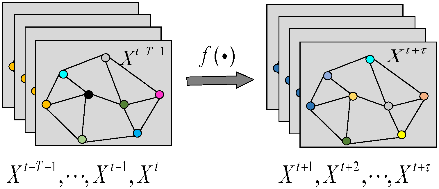
represents the number of features. Thus, the traffic prediction task aims to use the road network structure
and historical data from
time steps to estimate future traffic conditions at time
through a mapping function
, mathematically expressed as:
in the equation,
denotes the mapping function for traffic flow prediction. Thus, the objective is to estimate future traffic flow sequences
based on historical observations
using the predictive function. As shown in
Figure 1, the overall prediction process of the model is shown below.
3.2. General Model Architecture
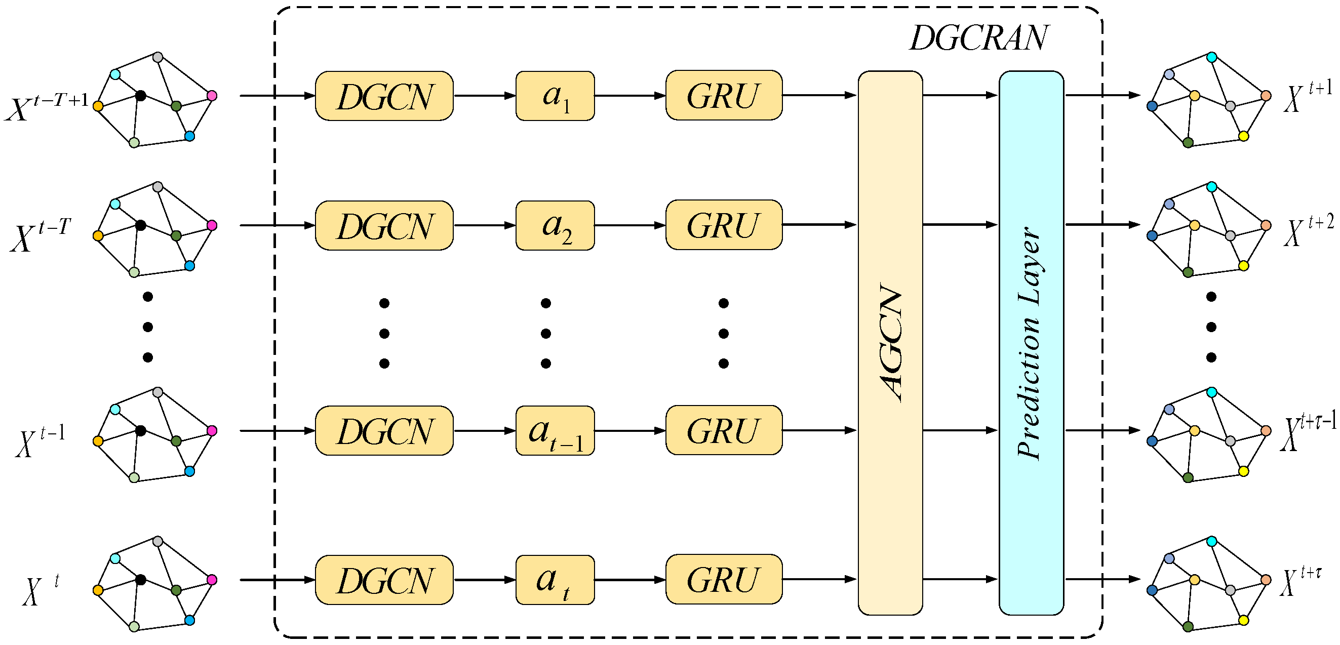
The overall architecture of the DGCRAN model is shown in
Figure 2. The combined model takes the time series of historical road network-wide nodes as inputs and uses the dynamic graph convolution module to initialize the node embedding, which in turn generates a similarity matrix for assessing the spatial correlation among nodes. In traffic and other road network related application scenarios, different colors in
Figure 2 represent nodes denoting historical traffic nodes with different attributes or functions, for example, they may be different types of road network nodes distinguishing between traffic hubs, common intersections, etc. In the traditional GRU framework, dynamic graph convolution operations are introduced to capture time-series features and spatial dependencies simultaneously. In addition, by constructing an adaptive graph convolution network, it is able to focus on different regions of the graph structure to extract complex associations in the graph more effectively. The model consists of the following two main components:
The Dynamic Graph Convolutional Recurrent Network (DGCRN) introduces a dynamic graph convolution mechanism for capturing potential hidden spatial dependencies. The network combines dynamic graph convolution with GRU to capture spatio-temporal correlation features of traffic flow more effectively.
Adaptive spatial feature extraction: spatial features are extracted to capture complex relationships in the graph structure more efficiently through the constructed adaptive graph convolutional network. This improves the model’s representational capability and enhances its predictive performance in complex scenarios.
3.3. Construction of Dynamic Graph Convolutional Recurrent Networks
In recent years, numerous researchers have focused on extracting spatially dependent features of spatio-temporal data using graph convolution techniques. However, these studies tend to construct predefined adjacency matrices through distance functions, which is a limitation of this approach and cannot adequately reflect the nodes’ own characteristics (e.g., POI, road structure and type) [
31]. Although traditional GCN simulates the spatial distribution of real traffic networks with the help of a predefined graph structure, its performance is limited by this fixed pattern. Although this structure can capture explicit similarity relationships between nodes, it is difficult to fully characterize the complex implicit associations prevalent in traffic data. This limitation results in the lack of spatial node association information, which reduces the accuracy of prediction. More importantly, the graph structures based on these methods are usually static, which makes it difficult to cope with the complexity and dynamically changing characteristics of spatial dependencies among nodes in real transportation networks.
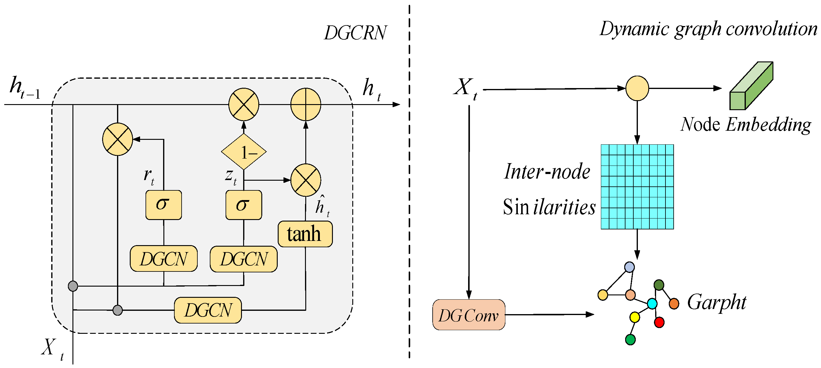
To address the above problems, a Dynamic Graph Convolutional Recurrent Network (DGCRN) is proposed for mining potential spatial features of traffic data, as shown in
Figure 3. The network incorporates GRU to efficiently capture spatio-temporal features. The DGCRN generates similarity matrix by initializing node embeddings and utilizes GCN to consider the unique patterns of nodes during feature aggregation. A DGCRN is constructed by integrating GRUs to automatically capture fine-grained spatio-temporal correlations in traffic sequences and dynamically update the parameters during training to adapt to traffic data in an end-to-end manner. In DGCRN, a supernetwork is designed to extract dynamic features using node attributes. The parameters of the dynamic filter are generated at each time step and the node embeddings are filtered to generate a dynamic graph. The two are very different in nature.
Traffic prediction involves complex temporal and spatial correlation features, and the DGCRN module is constructed by introducing GCN into the fully connected layer of GRU. Given the excellent performance of GRU in temporal tasks, graph convolution operations are integrated into its original architecture to capture temporal dynamic features and spatial dependencies simultaneously. In the model architecture, each time step receives not only the current input data, but also the hidden state of the previous moment, in order to regulate the store-and-forget mechanism of information. In this framework, GRU operations are applied in parallel to all nodes in the graph structure and the nodes share the same parameter settings.
Specifically, based on the input data
at time step
and the previous hidden state
, this paper formulates the single-step computation process of the gated recurrent unit as:
in the equation,
and
represent the input and output at time step, respectively,
,
, and
denote trainable parameters of the recurrent neural network,
indicates the sigmoid activation function, and
is used for dynamic graph generation.
The fusion of dynamic graph convolution with GRU enhances the model’s ability to capture fine spatio-temporal features. By adaptively constructing associations between nodes through the training data, this dynamically generated graph structure can break through the limitations of predefined graphs, resulting in more flexible handling of complex spatio-temporal patterns.
The application of dynamic graph convolution in traffic prediction has been gradually deepened, for example, EvolveGCN [
38] evolves the static graph weights through RNN, but its adaptability to sudden traffic changes is limited; DGCRN evolves the static graph weights through RNN, and its adaptation to sudden traffic changes is limited; DGCRN is more attuned to the instantaneous nonlinear nature of traffic data through an end-to-end dynamic adjacency matrix generation mechanism.
3.4. Adaptive Graph Convolutional Networks
In a traffic network, the traffic state of each road is affected by a variety of factors, and it is difficult to achieve accurate prediction only by obtaining the shared patterns among nodes. For this reason, adaptive neighbor matrix and node parameters are introduced to extract spatial features. The adaptive adjacency matrix captures potential spatial correlations in traffic data by automatically learning the dependencies between nodes; adaptive node parameters are generated from a shared pool of weights and biases to capture the unique patterns of specific nodes. Combining these two mechanisms, adaptive graph convolutional networks can extract spatial features of the data more comprehensively.
3.4.1. Adaptive Neighborhood Matrix
Adaptive Adjacency Matrix (AAM) is a dynamic adjacency matrix applied to graph neural networks. It continuously adjusts the matrix structure during stochastic gradient optimization by introducing an adaptive mechanism. Specifically, each row of the matrix represents a set of neighboring nodes of a node, and the row length corresponds to the degree of the node. The method not only effectively alleviates the sparsity problem, but also adapts to the dynamic changes in the number of nodes and edges in the graph. Through the data-driven approach, the adaptive adjacency matrix can learn the potential intrinsic associations between nodes and thus construct a more accurate representation of adjacencies. Predefined graph structures may not fully reflect spatial dependencies, which may lead to biased prediction results. In contrast, adaptive adjacency matrices do not rely on a priori knowledge and can learn the underlying spatial dependency patterns directly from the input data. The method described in reference [
14] captures the complete spatial correlation of traffic flow data by extracting spatial features, which can effectively improve the prediction accuracy. The specific implementation steps are as follows: First, a learnable embedding vector
is randomly generated for each node. Then, the spatial dependencies between nodes are derived using
and its transpose
. Finally, the normalized adaptive adjacency matrix can be expressed as:
in the equation, each row of
represents a node embedding. The total number of nodes is denoted as
, with the degree matrix
being a diagonal matrix. The adjacency matrix is represented as
. The
activation function is employed, while the adaptive adjacency matrix undergoes normalization via the softmax function. During training,
automatically adjusts to capture latent dependencies among different traffic flow sequences while simultaneously acquiring adjacency information required for graph convolution.
The phenomenon of gradient vanishing or gradient explosion can be effectively mitigated by constructing an adaptive adjacency matrix to capture the spatial dynamic dependencies among road networks more comprehensively. The graph convolution module is able to automatically learn the dynamically changing spatial dependencies in transportation networks without a priori information. The matrix is sparsified using
and normalized by
to directly obtain 3. The adaptive graph convolution in this model can be expressed as:
3.4.2. Adaptive Node Parameter
In transportation networks, the dynamic nature of time-series data and the various factors that nodes may be affected by lead to diverse patterns among different traffic sequences. Therefore, it is difficult to achieve accurate traffic prediction by capturing only the common patterns among nodes. Since the characteristics of neighboring nodes in the road network structure may exhibit different traffic conditions at a certain time due to specific attributes (e.g., weather, accidents), even the characteristics of non-neighboring nodes may show opposite trends. Therefore, relying only on the shared patterns among all nodes cannot ensure the accuracy of prediction, and it is especially important to allocate an independent parameter space for each node to learn its unique patterns. Typically, graph convolutional networks are computed as:
in the equation,
represents the adjacency matrix of the graph, while
and
denote the input and output matrices, respectively. The trainable weight matrix
and bias vector
complete the parameter set.
To address the issue where assigning independent parameters to each node leads to an excessively large
that is difficult to optimize, we enhance traditional GCN through a node-adaptive parameter learning module. For the adaptive node parameters, we define a node-embedding matrix
and a weight pool
, where
is the embedding dimension with
, yielding
. From a node’s perspective, this process extracts candidate patterns from all traffic sequences while learning node-specific patterns—specifically, node embedding
retrieves parameters
for node
from the shared weight pool
, with analogous operations for
. The GCN formulation incorporating adaptive node parameters is as follows:
4. Experimental Design and Analysis
4.1. Dataset Description
To validate the accuracy of the model, experiments were conducted on the publicly available PEMS03, PEMS04, and PEMS08 datasets. The PEMS database integrates traffic data collected by the California Department of Transportation on highways and includes informational data from other California transportation agencies and partners. The database provides users with a comprehensive assessment of highway performance. By monitoring the real-time status of the highway network, users can make more informed operational decisions, analyze congestion bottlenecks, and identify potential improvements. In addition, the data helps to develop more effective overall traffic management strategies, thereby improving the efficiency and sustainability of the transportation system. The PEMS03 dataset contains freeway information recorded by 358 traffic detection sensors in the Los Angeles freeway region between 1 September and 30 November 2018. The PEMS04 dataset covers freeway data collected by 307 sensors in San Francisco between 1 January and 28 February 2018. The PEMS08 dataset is from the San Bernardino region and records freeway information collected between 1 July and 31 August 2016 by 170 sensors. Traffic flow data from these datasets are summarized every 5 min, with more details shown in
Table 1. The following is a link to download the dataset:
https://gitcode.com/open-source-toolkit/06a2f (accessed on 25 June 2025)
The missing values in the dataset are linearly interpolated and normalized to ensure the stability of the training process. In the dataset, all the historical data of 12 time steps are used to predict the traffic flow for the next 12 time steps. The dataset was divided into training, validation, and test sets in the ratio of 6:2:2. The optimization process was performed using the Adam optimizer, which is well suited for handling large-scale data and parameters due to its high computational efficiency and low memory requirements. The training setup consists of 200 iterations with a bit size of 64, an initial learning rate of 0.001, and the application of an early stopping method with a patience of 15.
4.2. Evaluation Metrics and Baselines
To evaluate the effectiveness of DGCRAN, we used three performance metrics that are widely used in traffic prediction tasks to compare the performance of different models.
- 2.
Root Mean Square Error (RMSE):
- 3.
Mean Absolute Percentage Error (MAPE):
in the equation,
denotes the total number of samples,
represents the ground truth value of the
-th sample, and
indicates the predicted value for the
-th sample. The prediction error is evaluated using MAE, RMSE, and MAPE metrics, where lower values correspond to better prediction performance.
In order to verify the prediction effect of DGCRAN model, 15 prediction models were selected as benchmark comparison models in this paper as follows:
HA [
9]: modeling traffic as a seasonal process and traffic flow based on the average of previous seasons as historical data.
VAR [
9]: time-series modeling that captures the spatial correlation between all traffic sequences.
DSANet [
39]: a correlated time-series prediction model that captures the temporal correlation between time series and spatial correlation using a CNN network and a self-attention mechanism.
DCRNN [
15]: diffusion convolution recurrent neural network which formulates the graph convolution and diffusion process and combines the GCN with a recurrent model in an encoder–decoder fashion for multi-step prediction.
ASTGCN [
14]: an attention-based spatio-temporal graph convolutional network that further integrates spatio-temporal attention mechanisms into STGCN to capture dynamic spatio-temporal patterns for modeling traffic data.
LSGCN [
40]: using gated graph blocks to satisfy the spatial dependence of long and short distances, which contains a graph convolutional network and a new cosine graph attention network.
STSGCN [
32]: spatio-temporally synchronized graph convolutional network captures spatio-temporal correlations by superimposing multiple local GCN layers and adjacency matrices on the time axis.
AGCRN [
14]: integrating the adaptive GCN of graphs into a recurrent network based on codec architecture for modeling.
STFGNN [
16]: designing a dynamic time-warping-based temporal graph to mine spatial relationships in function perception.
STGODE [
17]: solved the GCN over-smoothing problem using CGNN to extract spatio-temporal dependencies.
Z-GCNETs [
41]: introduces the concept of sawtooth persistence for time-series prediction;
STG-NCDE [
30]: predicting traffic volumes using two neural control differential equations.
DSTAGNN [
35]: simulates dynamic spatial relationships between nodes by designing a spatio-temporal perceptual graph and mines historical traffic flow data of nodes using an attention mechanism.
DDGCRN [
8]: extracts dynamic spatio-temporal features of traffic data using spatio-temporal embedding and dynamic signals to capture the spatio-temporal correlation of traffic data.
PDG2Seq [
42]: extracts dynamic real-time traffic spatio-temporal features using the Periodic Feature Selection Module (PFSM) and Periodic Dynamic Graph Convolutional Gated Recurrent Unit (PDCGRU) to accurately predict traffic flow.
4.3. Forecasting Performance Comparison
The results of the comparison experiments between the DGCRAN model and the benchmark model on the PEMS03, PEMS04, and PEMS08 datasets are shown in
Table 2. First, traditional time-series analysis methods (e.g., HA and VAR) tend to have poor prediction performance, indicating limitations in handling nonlinear and complex traffic data. HA performs the worst of all models, setting the minimum standard for traffic prediction. In addition, VAR and DSANet yielded much worse results than neural network-based models because they cannot effectively capture nonlinear dependencies and require manual design of features. Second, in graph-based models, DCRNN relies on predefined graph structures to capture spatial correlations. However, the quality of the predefined graph structure has a significant impact on the final performance of the model. ASTGCN and LSGCN perform well in extracting dynamic relationships in traffic time series, proving their effectiveness. STFGNN and STGODE extend the spatial sensory field by introducing temporal graphs and GODE, outperforming other graph-based methods. However, they are deficient in mining global spatial correlation and thus inferior to the AGCRN model. Models such as AGCRN, STFGNN, and DSTAGNN achieve significant results by generating graph structures to extract spatial features in a data-driven manner. However, these models do not fully consider the periodic characteristics and dynamic signals of the traffic system, resulting in inferior performance to DGCRAN. Although DDGCRN utilizes dynamic graphs to extract spatial features, it only focuses on the temporal information of the input data and ignores the temporal information of the prediction target. In contrast, DGCRAN makes full use of the temporal information of the predicted target and thus outperforms DDGCRN.PDG2Seq predicts by capturing the spatio-temporal characteristics of dynamic real-time traffic, but it still does not perform as well as DGCRAN.
In conclusion, DGCRAN demonstrates lower MAE, RMSE, and MAPE metrics on the three datasets compared to other traffic flow prediction models, proving its superiority in prediction accuracy and capability. Compared with the traditional HA and VAR models, the MAE of DGCRAN on the PEMS08 dataset is reduced by 21.33% and 5.66%, respectively; the RMSE is reduced by 46.02% and 6.59%, respectively; and the MAPE is reduced by 19.02% and 4.24%, respectively. This indicates that the deep learning-based prediction method significantly improves the accuracy compared to the traditional statistical model. Compared with other models, DGCRAN introduces graph convolution operation into the original GRU structure to capture the time-series information and constructs an adaptive graph convolution network. This not only makes the model closer to the actual situation when extracting spatial features, but also gives different weights to the spatio-temporal features for different time periods, better reflecting the changing pattern of daily traffic flow, thus further improving the accuracy of prediction.
4.4. Comparison of Prediction Time Steps
In order to assess the prediction accuracy of the models and their trends at different time steps, we performed a comparative analysis of the prediction results of DGCRAN, DSTAGNN, AGCRN, and STGODE on the PEMS04 and PEMS08 datasets. As shown in
Figure 4, the MAE, RMSE, and MAPE of all models show an increasing trend as the prediction time horizon is extended, which is consistent with the expectation that the prediction difficulty increases with the expansion of the horizon. It is worth noting that although STGODE performs poorly in short-term prediction, its error grows significantly faster than the other models, resulting in the highest average error. DSTAGNN performs similarly to AGCRN in long-term prediction, but outperforms the latter in short-term prediction, showing its advantage in short-term prediction. In contrast, DGCRAN is able to automatically capture fine-grained spatio-temporal correlations in traffic sequences by freeing itself from the constraints of predefined graphs, thus demonstrating a significant performance advantage. Overall, DGCRAN outperforms the other models at different time steps, demonstrating its higher accuracy, stability and reliability in the prediction task.
4.5. Ablation Study
In order to validate the effect of dynamic graph convolution and AGCN in the proposed model, multiple variants of the model were constructed by removing or replacing some of the modules and tested on the PEMS04 and PEMS08 datasets. The ablation experiments cover the following variants:
- (1)
GCGRU: As a benchmark model for ablation experiments, the graph-convolution gated recurrent unit (GCGRU) combines classical GCN and GRU to capture spatio-temporal dependencies.
- (2)
DGCRN: This model uses Dynamic Graph Convolutional Network (DGCN) instead of the traditional GCN to construct Dynamic Graph Convolutional Recurrent Network. By initializing node embeddings to generate similarity matrices, DGCN takes into account the unique characteristics of nodes in the feature aggregation process, thus escaping from the limitation of predefined graphs. The combination of GRU further enhances the model’s ability to model fine-grained spatio-temporal patterns.
- (3)
No adaptive graph convolution (w/o adaptive DGCRAN): In this variant, the adaptive graph convolution module is removed and a simple graph convolution is used instead.
The results of the ablation experiments on the PEMS04 and PEMS08 datasets are shown in
Table 3. First, DGCRN outperforms GCGRU as a whole, indicating that dynamic graph convolution is able to break through the limitation of predefined graphs and effectively capture spatial dependencies. DGCRN dynamically generates the adjacency matrix through the hypernetwork, and accurately reflects the real-time correlation strength between nodes by utilizing the multidimensional information of the input data such as the features at the current moment, the temporal data, and the hidden state of the previous moment, to achieve a Dynamic Capture. Secondly, the prediction performance of the model is not as good as that of DGCRAN when using an ordinary graph convolution neural network instead of adaptive graph convolution, which indicates that ordinary graph convolution is limited by the fixed graph structure, and it is difficult to adapt to the complex spatial relationship of traffic network. On the other hand, DGCRAN generates adaptive neighbor matrix in real time during the training process through the node-embedding technology, which can keenly capture the correlation changes between road sections in different time periods and fully explore the spatial dynamic correlation, proving the effectiveness of the adaptive graph convolution module. Overall, the DGCRAN model outperforms GCGRU and DGCRN, indicating that the synergistic effect of DGCRN and AGCN is crucial to the model prediction results. The graph structure is optimized by AGCN to effectively extract features and accurately capture key information of the graph data, which improves the accuracy and robustness of the prediction.
4.6. Embedding Dimensional Analysis
In DGCRAN, the embedding dimension of a model node is a crucial parameter, the size of which directly determines the model’s ability to extract spatio-temporal information. The PeMSD4 and PeMSD8 datasets are used as test subjects, and the embedding dimensions are set to 3, 6, 9, 12, 15 and 4, 6, 8, 10, 12, respectively. The MAE and MAPE values of DGCRAN in the 12-step prediction interval are shown in
Figure 5. The following experimental data are the average values of each evaluation metric in the 12-step prediction interval. As can be seen from
Figure 5, there is a significant difference in the performance of the model at different embedding dimensions. Excessive or insufficient embedding dimensions can adversely affect the performance of the model. Although a larger embedding dimension can contain more data information, it also leads to an increase in model parameters, which increases the difficulty of model optimization.
In summary, for the PeMSD4 dataset, when the embedding dimension is set to 12, the MAE and MAPE values are closest to the real evaluation values, at which time DGCRAN is able to achieve the best performance; while for the PeMSD8 dataset, when the embedding dimension is set to 8, the MAE and MAPE values are closest to the real evaluation values, at which time DGCRAN is also able to achieve the best performance.
4.7. Calculation Cost Analysis
In order to evaluate the computational cost, the number of parameters and training time of DGCRAN are compared with four models, DCRNN, STGCN, ASTGCN, and AGCRN, on the PEMS04 dataset, as shown in
Table 4. In terms of the number of parameters, DGCRAN exceeds DCRNN and STGCN when the node embedding dimension of DGCRAN is set to 12. This is due to the fact that the node-embedding dimension is added as a cost of learning node-specific patterns in order to better capture specific node patterns; ASTGCN introduces a spatio-temporal attention mechanism to obtain more accurate spatio-temporal features, but it also increases the number of parameters and training time. AGCRN uses an adaptive convolutional recursive algorithm that increases the number of model parameters. In terms of training time, AGCRN runs slightly faster than DCRNN because the model generates all predictions directly instead of using the iterative approach in DCRNN. STGCN is the fastest due to the temporal convolution structure that accelerates model training; ASTGCN has a higher number of parameters and training time due to the fact that it requires a higher number of parameters and training time to introduce spatial and temporal attention mechanisms to learn more accurate spatio-temporal patterns.
When the embedding dimension of DGCRAN is 6, the number of modeled parameters is less than DCRNN, STGCN, ASTGCN, and AGCRN, and the training time and RMSE values are also lower. When the embedding dimension is 12, DGCRAN has less number of parameters than ASTGCN and AGCRN and the smallest RMSE value, but the training time is slightly longer, which is due to the fact that the model contains a stack of three DGCN modules, which enhances the extraction of temporal information but also increases the computational complexity. Overall, considering the number of parameters and prediction accuracy together, the prediction effect of DGCRAN is better when the embedding dimension is 12, and the computational cost is more reasonable.
5. Discussion
The DGCRAN model proposed in this study achieves significant performance improvement in the traffic flow prediction task through the co-design of dynamic graph convolution and adaptive spatial feature extraction. From a broader perspective, this study has three implications for the development of intelligent transportation systems: first, the dynamic graph generation mechanism provides a generalized framework for dealing with non-smooth spatio-temporal correlations, which can be extended to areas such as air quality prediction and crowd flow monitoring. Second, the adaptive parameter learning module provides a new idea to solve the problem of node heterogeneity in graph data, which has inspirational value for scenarios such as social network analysis. Third, the stability of the model in long-term prediction indicates its potential for practical deployment, which can provide more reliable decision support for urban traffic management. Compared with the literature [
37,
38], the DGCRAN model has a wider applicability in terms of the dynamic graph generation mechanism, and is able to automatically adapt to the spatial and temporal variations in different traffic scenarios. However, the task-driven graph learning framework and real-time interactive modeling approach proposed in these studies provide important insights for future research, especially in multimodal data fusion and lightweight design.
It is worth noting that the current work still suffers from two limitations: on the one hand, the model’s adaptability to contingencies has not been specifically tested, which is crucial in practical applications. On the other hand, the sensitivity issue of the node-embedding dimension suggests the need to develop more efficient parameter compression techniques.
Analyzing from the perspective of future research, the following directions can be explored in depth: (1) Developing multimodal dynamic graph architectures that incorporate external factors (e.g., weather, events) to enhance the scenario adaptability of the model. (2) Investigating a lightweight version to reduce the computational cost to make it suitable for edge device deployments. (3) Incorporating causal inference techniques to enhance the interpretability of the model, which is crucial for traffic management decisions. In addition, the dynamic graph convolution paradigm proposed in this paper provides a new experimental vehicle for the theoretical study of spatio-temporal graph neural networks, especially in the fusion mechanism between dynamic graph representation learning and traditional temporal modeling, which is worthy of deeper exploration. The development of these directions will further promote the transformation of traffic prediction from laboratory research to practical applications in smart cities.
The DGCRAN model performs excellently in traffic flow prediction experiments, and its innovative architecture enables it to effectively capture spatio-temporal dependencies, solve the problem of heterogeneous traffic patterns, and outperforms the benchmark model in predictions at different time steps. This not only provides support for intelligent transportation systems, but also promotes research in the field of traffic prediction. Based on this, it is recommended to pilot the application in practical traffic management and expand the research with other techniques. However, the model suffers from untested adaptation to unexpected events and a sensitive node-embedding dimension. In the future, the performance should be evaluated by simulating unexpected events, and the model should be improved both in terms of optimizing the structure and adopting compression algorithms in order to enhance the model’s practicality.
6. Conclusions
The DGCRAN model proposed in this paper uses a novel combination of dynamic graph convolution and GRU to construct a dynamic graph convolution recurrent network. It breaks through the limitation of traditional GCN relying on predefined static graphs through end-to-end generated dynamic neighbor matrix, and is able to capture the real-time changing spatio-temporal correlations in the traffic network. Second, Adaptive Graph Convolutional Network (AGCN) achieves the modeling of personalized node features through node embedding technique, which solves the problem of heterogeneous traffic patterns that are difficult to be handled by traditional methods. Finally, the synergy of the dual modules enables the model to capture global spatio-temporal dynamics as well as focus on local feature differences.
Through various experiments on the PEMS03, PEMS04, and PEMS08 datasets, the traffic prediction ability of the DGCRAN model was demonstrated to be superior to existing methods. In future work, the DGCRAN model can be combined with other deep learning methods to better learn the spatio-temporal features hidden in the traffic data for more accurate predictions.


